By Sarita Jondhale 1

• The process of removing the formants is called inverse filtering

• The remaining signal after the subtraction of the filtered modeled signal is called the residue

• The number which describe the intensity and frequency of the buzz, the formants, and the residue signal, can be stored or transmitted

By Sarita Jondhale 2

Encoding the residueEncoding the residue• Most successful method is a use of

codebook• Codebook: is a table of typical

residue signals, which is set up by the system designers

• Analyzer compares the residue to all the entries in the codebook, chooses the entry which is the closest match, and just send the code for that entry

By Sarita Jondhale 3

• The synthesizer receives this code, retrieve the corresponding residue form the codebook, and uses that to excite the formant filter

By Sarita Jondhale 4

Vector QuantizationVector Quantization

• A technique of compressing the data• The basic idea of VQ is to reduce the

information rate of the speech signal to a low rate through the use of a codebook with a relatively small number of code words

By Sarita Jondhale 5

Vector QuantizationVector Quantization

• The output of both filter bank and LPC analysis is in the form of vectors

• The main idea in VQ is to make vectors look like symbols that we can count

• The VQ is nothing more than an approximator

By Sarita Jondhale 6

Vector QuantizationVector Quantization

-4 -3 -2 -1 0 1 2 3 4

00 01 10 11

Example of 1-dimensional VQ

• Every number less than -2 is approximated to -3 and so on..

• The approximate values are uniquely represented by 2 bits

• VQ has rate of 2bits/dimension

By Sarita Jondhale 7

Vector QuantizationVector Quantization• Advantages:

– Reduced storage for spectral analysis information

– Very efficient– Reduced computation for determining

similarity of spectral analysis vectors. – Discrete representation of speech sounds

By Sarita Jondhale 8

Vector QuantizationVector Quantization• Disadvantages:

– An inherent spectral distortion in representing the actual analysis vector: as the size of the codebook increases, the size of the quantization error decreases and vice versa

– The storage required for the codebook is important: larger the codebook lesser the quantization error but more the storage required for the codebook

By Sarita Jondhale 9

Vector QuantizationVector Quantization

• Create a training set of feature vectors • Cluster them into a small number of

classes• Represent each class by a discrete symbol

By Sarita Jondhale 10

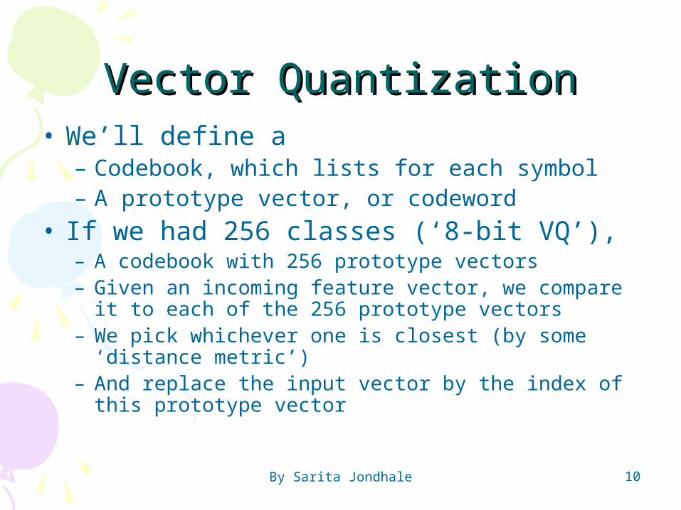
Vector QuantizationVector Quantization• We’ll define a

– Codebook, which lists for each symbol– A prototype vector, or codeword

• If we had 256 classes (‘8-bit VQ’),– A codebook with 256 prototype vectors– Given an incoming feature vector, we compare it to

each of the 256 prototype vectors– We pick whichever one is closest (by some

‘distance metric’)– And replace the input vector by the index of this

prototype vector

By Sarita Jondhale 11

Vector QuantizationVector Quantization

By Sarita Jondhale 12

Vector QuantizationVector Quantization• A distance metric or distortion metric

– Specifies how similar two vectors are

By Sarita Jondhale 13

Vector QuantizationVector Quantization• Simplest:

– Euclidean distance

– Also called ‘sum-squared error’

d(x,y) (x i y i)2

i1

D

By Sarita Jondhale 14

Vector QuantizationVector Quantization• Vector classification procedure: is basically

a full search through the codebook to find the “best” match

• Best match: The quantization error is minimum

By Sarita Jondhale 15

How does VQ work in compression?

• A vector quantizer is composed of two operations.  – encoder– decoder. 

By Sarita Jondhale 16

encoderencoder• The encoder takes an input vector and

outputs the index of the codeword that offers the lowest distortion. 

• In this case the lowest distortion is found by evaluating the Euclidean distance between the input vector and each codeword in the codebook. 

• Once the closest codeword is found, the index of that codeword is sent through a channel

• the channel could be a computer storage, communications channel, and so on

By Sarita Jondhale 17

decoderdecoder• When the decoder receives the index

of the codeword, it replaces the index with the associated codeword. 

By Sarita Jondhale 18

Figure 2: The Encoder and decoder in a vector quantizer.  Given an input vector, the closest codeword is found and the index of the codeword is sent through the channel.  The decoder receives the index of the codeword, and outputs the codeword.

By Sarita Jondhale 19

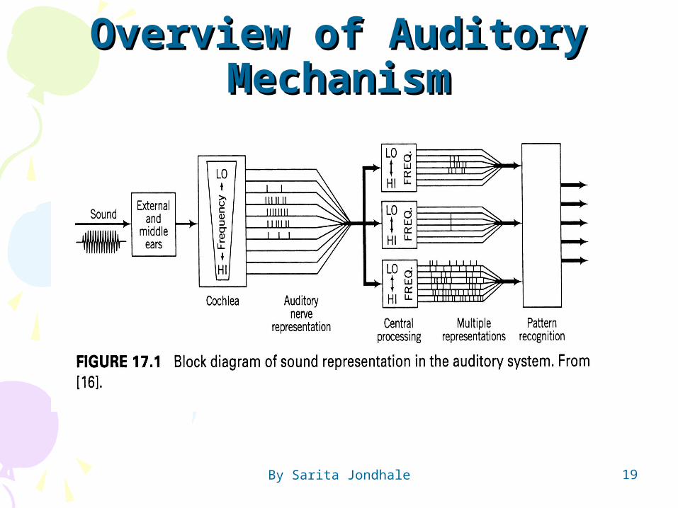
Overview of Auditory Overview of Auditory MechanismMechanism

By Sarita Jondhale 20

Schematic Schematic Representation of the Representation of the

EarEar

By Sarita Jondhale 21

Sound perceptionSound perception

• The audible frequency range for human is apprx 20Hz to 20KHz

• The three distinct parts of the ear are outer ear, middle ear and inner ear

Outer ear: pinna and Auditory(external) canal

Middle ear: tympanic membrane or eardrum

Inner ear: cochlea, neural connections

By Sarita Jondhale 22

Outer ear: pinna and Auditory(external) canal

Middle ear: tympanic membrane or eardrum

Inner ear: cochlea, neural connections

By Sarita Jondhale 23

• Outer ear:– Outer ear includes pinna and auditory

canal– It helps to direct an incident sound

wave into middle ear– Filters and modifies the captured

sound– The perceived sound is sensitive to the

pinna’s shape – By changing the pinnas shape the

sound quality alters as well as background noise

– After passing through ear cannal sound wave strikes the eardrum which is part of middle ear

By Sarita Jondhale 24

• Middle ear– Ear drum:

• This oscillates with the frequency as that of the sound wave

• Movements of this membrane are then transmitted through the system of small bones called as ossicular system

• From ossicular system to cochlea• Cochlea achieves efficient form of

impedance matching

By Sarita Jondhale 25

• Inner ear– It consist of two membranes Reissner’s

membrane and basilar membrane– When vibrations enter cochlea they

stimulate 20 000 to 30 000 stiff hairs on the basilar membrane

– These hair in turn vibrate and generate electrical signal that travel to the brain and become sound

– The resonance of the basilar membrane identifies the sound frequency

– The intensity of the sound is direct translation of the amplitude of the basilar membrane into excitation of hair cells which in turn fire at higher rates

By Sarita Jondhale 26

Pinna Auditory cannal

ossicular system

cochlea

Basilar membrane

Tympanic membrane

By Sarita Jondhale 27

Basilar Membrane MechanicsBasilar Membrane Mechanics

By Sarita Jondhale 28

Basilar Membrane Basilar Membrane MechanicsMechanics

• Characterized by a set of frequency responses at different points along the membrane

• Different regions of the BM respond maximally to different input frequencies => frequency tuning occurs along BM

• Mechanical realization of a bank of filters

• Distributed along the Basilar Membrane is a set of sensors called Inner Hair Cells (IHC) which act as mechanical motion-to-neural activity converters

By Sarita Jondhale 29

• Mechanical motion along the BM is sensed by local IHC causing firing activity at nerve fibers that innervate bottom of each IHC

• Each IHC connected to about 10 nerve fibers, each of different diameter =>– thin fibers fire at high motion levels,– thick fibers fire at lower motion levels

• 30,000 nerve fibers link IHC to auditory nerve

• Electrical pulses run along auditory nerve, ultimately reach higher levels of auditory processing in brain, perceived as sound

By Sarita Jondhale 31

Auditory modelAuditory model• It is the implementation of human Auditory model

to machines• The auditory model consists of stages for the

outer, middle and inner ears.• The output of the auditory model is the ensemble

interval histogram (EIH) which shares similarities to the auditory nerve response of the mammalian ear.

• Spectral estimation using auditory models has shown to be efficient and robust

• but the success of the system depends on the accuracy and robustness of the auditory model used.

By Sarita Jondhale 32

EIH modelEIH model• It is a frequency-domain representation,

which gives fine low-frequency detail and a grater degree of robustness than conventional spectral representations.

• The representation is formed from the ensemble histogram of inter-spike intervals in an array of auditory nerve fibers.

• Useful in isolated word recognition

By Sarita Jondhale 33

Ensemble Interval Histogram Ensemble Interval Histogram (EIH(EIH))

By Sarita Jondhale 34

• First stage of linear filters • The second stage takes the output of each filter

and computes the intervals between the positive crossings of the filtered waveform at various logarithmically spaced thresholds.

• A histogram of the frequencies corresponding to these intervals is then created.

• The final stage combines the histograms for each of the channels together into the; final output, the Ensemble Interval Histogram.