by - Welcome to DORAS - DORAS - DCUdoras.dcu.ie/17342/1/lorna_M._fanning_20120702114452.pdf · kd...

THE DEVELOPMENT AND APPLICATIONS OF

POLYCLONAL AND MONOCLONAL ANTIBODIES FOR

THE DETECTION OF ILLICIT DRUGS IN SALIVA

SAMPLES

A thesis submitted for the degree of

Doctorate of Philosophy

byLorna M. Fanning B.A.(Mod), M.Sc.

September 2002

Under the supervision of Professor Richard O’Kennedy

Based on research carried out at

School of Biotechnology,

Dublin City University,

Dublin 9,

Ireland.

Declaration

I hereby certify that this material, which I now submit for assessment on the programme

of study leading to the award of Doctor of Philosophy, is entirely my own work and has

not been taken from the work of others save and to the extent that such work has been

cited and acknowledged within the text of my work.

Signed: j? ID No.:

Date: d \ S a p t '0 0 .

AcknowledgementsSincere thanks to Prof. Richard O'Kennedy for his guidance and support throughout this

project. Thanks to the following for their support and assistance:

• Members of the SMT Project Group from Envitec, Nunc, and University o f Gent

• Dr. Bridin Brady, State Laboratory, Dublin

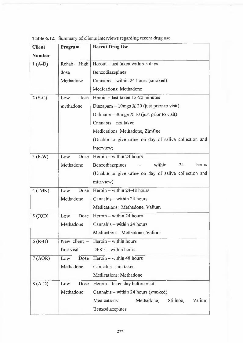
• Dr. Eamon Keenan, staff and clients of Trinity Court Drug Treatment Centre

Thanks to my lab colleagues at DCU for their help (especially Joanne for her help with

sample collection and Stephen for his help with the cells).

Thanks to my friends, especially 'the girls' for all the fun throughout the years. Thanks

also to my family Ailbhe, Joe, Carmel, Brig, Andy, Mary and Andy. Special thanks to

Mam and Dad for everything!

Publications

Fitzpatrick, J., Fanning. L., Hearty, S., Leonard, P., Manning, B.M., Quinn, J.G., and

O’Kennedy, R. (2000). Applications and recent developments in the use of antibodies

for analysis. Anal. Letts, 33:2563-2609.

Fanning, L. and O’Kennedy, R. (2002). Developments in rapid immunological-based

methods of detection of illicit drugs in saliva samples. In Preparation. TRAC

Fanning, L. and O’Kennedy, R. (2002). Development and characterisation of anti

amphetamine and anti-methamphetamine monoclonal antibodies and application for

detection of amphetamines in saliva samples. In Preparation. J. Immunol. Meth.,

Abstract

Anti-tetrahydrocannabinol (THC), anti-cocaine and anti-morphine polyclonal antibodies

were produced. These antibodies were successfully applied to an ELISA format for the

detection of THC, cocaine, and morphine in saliva samples.

Monoclonal antibodies against amphetamine and its derivatives were produced using

two different conjugates, amphetamine-bovine serum albumin and methamphetamine-

bovine serum albumin. Two successful clones were produced, and the antibodies were

applied to an ELISA format for the detection of amphetamine, methamphetamine, and

the other common amphetamine derivatives, such as methylenedioxyamphetamine

(MDA) and methylenedioxymethamphetamine (MDMA). The ELISA was developed

using saliva as the matrix. During the screening stage of the production of these

antibodies, particular attention was given to their cross reactivity profiles. Among the

molecules tested for cross-reactivity, were legally available medications such as

ephedrine, as other commercially available antibodies show cross reactivity. The

resulting monoclonal antibodies detected amphetamine and other designer derivatives,

and showed negligible cross reactivity with the legal structurally related molecules.

The antibodies were applied to a biosensor (BIAcore) assay for the detection of

amphetamine and methamphetamine in saliva samples. The affinity constants for the

antibodies were determined by ELISA and BIAcore methods. The values obtained

were found to be similar by both methods.

A novel automated prototype device, developed by our collaborators, Envitec, was

optimised and the anti-THC polyclonal antibody was applied to it for the screening of

saliva samples for the presence of THC. This was a rapid, qualitative test, and it could

be performed in less than 20 minutes. The basis of the assay was competition between

horseradish peroxidase-labeled THC and THC present in the saliva samples, for binding

to the anti-THC polyclonal antibodies that coated the reaction wells of the device.

AbbreviationsAPC antigen presenting cell

BDB benzodioxole-5-butanamine

BEC benzoylecgonine

BIA biomolecular interaction analysis

BSA bovine serum albumin

BtG bovine thyroglobulin

CDR complementarity determining regions of antibody

CE capillary electrophoresis

CV coefficient of variation

DNA deoxyribonucleic acid

EDC N-ethyl-N'-(dimethylaminopropyl) carbodiimide

EDTA ethylenediaminetetra acetic acid

EME ecgonine methyl ester

ELISA enzyme-linked immunosorbent assay

EMIT enzyme-multiplied immunoassay technique

Fab binding region of antibody above the hinge region

Fc constant region of antibody molecule

FCS foetal calf serum

FPIA fluorescence polarisation immunoassay

Fv variable binding fragment of antibody

GC/MS gas chromatography/mass spectroscopy

HAT hypoxanthine aminopterin thymidine

HPLC high performance liquid chromatography

HT hypoxanthine thymidine

HBS Hepes buffered saline

IgG immunoglobulin class G

IgA immunoglobulin class A

IgD immunoglobulin class D

IgE immunoglobulin class E

IgM immunoglobulin class M

k a equilibrium association affinity constant

ka association rate constant

vi

Kd equilibrium dissociation affinity constant

kd dissociation rate constant

MAb monoclonal antibody

MDA 3,4-methylenedioxyamphetamine

MDMA 3,4-methylenedioxymethamphetamine

MBDB 3,4-methylenedioxyphenyl-2-butanamine

MDEA 3,4-methylenedioxy-N-ethylamphetamine

MW molecular weight

NEAA non-essential amino acids

NIDA National Institute of Drugs of Abuse

NHS N-hydroxysuccinimide

OVA ovalbumin

PAGE polyacrylamide gel electrophoresis

PBS phosphate buffer saline

PEG polyethylene glycol

pH log of the hydrogen ion concentration

SAMHSA Substance Abuse and Mental Health Service

Administration

scFv single chain Fv antibody derivative

SE standard error

SDS sodium dodecyl sulphate

SMT Standard, Measurements and Testing Framework

S/P saliva/plasma ratio

SPR surface plasmon resonance

THC tetrahydrocannabinol

THC-COOH tetrahydrocannabinol carboxylic acid

THY thyroglobulin

UV ultraviolet

Vh variable region of heavy chain

Vl variable region of light chain

WHO World Health Organisation

vii

Units

°c degrees Celcius

cm centimetres

g grams

KDa kilodaltons

Kg kilogram

1 litre

Mg microgram

III microlitre

pM micromolar

M molarmg miligrammin minuteml millilitremm millimetresnm nanometrenM nanomolar

mol molarrpm revolutions per minuteRU response unitssec, s secondsv/v volume per unit volumew/v weight per unit volume

Table of Contents:

Declaration «

Acknowledgements Hi

Publications >v

Abstract v

Abbreviations vi

Units viii

Chapter 1

Introduction 11.1 Drugs of abuse in saliva - Background 2

1.1.1 Saliva as a matrix 2

1.1.2 pH of saliva and influence on drug concentrations 5

1.2 Other alternative biological matrices 6

1.3 Legal status of alternative biological matrices 10

1.4 Drugs of abuse: metabolism, form and concentrations 11

found in saliva

1.4.1 Cocaine 11

1.4.2. Tetrahydrocannabinol 15

1.4.3 Amphetamines 17

1.4.4. Opioids 22

1.5 Levels of detection of assays and cut-off levels 25

1.6. Methods of detection of drugs of abuse 26

1.6.1 Immunoassays 26

1.6.1.1 Competitive Immunoassay 27

1.6.1.2 Non-Competitive Immunoassay 27

1.6.2. Enzyme-Multiplied Immunoassay Technique 32

1.6.3 Fluorescence Polarisation Immunoassay 32

ix

1.6.4 Detection of analytes by immunoassay using up-converting phosphor

technology 32

1.6.5 Agglutination 33

1.6.6 Biosensors 33

1.7 Commercials Tests 36

1.8 Summary of Introduction 40

1.9 Aims of Thesis 41

Chapter 2

Materials & Methods 432.1 Materials 44

2.2 Equipment 46

2.3 Consumables 47

2.4 Standard Solutions 48

2.4.1 Cell culture media 48

2.4.2. SDS PAGE Solutions 49

2.5 Production of drug-protein conjugates 50

2.5.1 Conjugation of morphine-3-glucuronide to protein 50

2.5.2 Conjugation of cocaine to protein 50

2.5.3 Commercial conjugates 51

2.6 Immunisations for polyclonal and monoclonal

antibody production 51

2.6.1 Immunisation protocol for the production of monoclonal antibodies 51

2.6.2. Immunisation protocol for the production of monoclonal antibodies 52

2.6.3 Preparation of rabbit serum 53

2.6.4 Preparation of mouse serum 53

2.7 Production of monoclonal antibodies 53

2.7.1 Cell lines 53

2.7.2 Immunisation schedule 54

2.7.3 Fusion 54

2.7.4 Screening of hybridoma supernatants 55

2.7.5 Storage of cell lines 55

2.7.6 Mycoplasma screening 55

2.8 Purification and Characterisation of antibodies 56

2.8.1. Purification of polyclonal rabbit serum 56

2.8.1.1 Ammonium sulphate precipitation 56

2.8.2 Monoclonal Antibody Purification 56

2.8.2.1 Concentration of tissue culture supernatant 56

2.8.3 Protein G Affinity Column 57

2.8.4 Sodium Dodecyl Sulphate-Polyacrylamide Gel Electrophoresis 57

2.8.5 Determination of Protein Concentration - BCA 57

2.9. Immunoassays 58

2.9.1. Estimation of rabbit antibody titre 58

2.9.2. Estimation of mouse antibody titre 59

2.9.3. Non-competitive enzyme-linked immunosorbent assay for 59

determination of antibody titre and optimal concentration of

protein conjugates

2.9.4 Competitive enzyme-linked immunosorbent assay 59

2.9.5 Isotyping of monoclonal antibodies 60

2.9.6 Affinity analysis ELISA - Friguet method 61

2.9.7 Determination of immunoglobulin concentrations by affinity capture 61

ELISA

2.10 BIAcore Studies 62

2.10.1 Preconcentration studies 62

2.10.2 Immobilisation of drug-protein conjugates 62

2.10.3 Regeneration studies 62

2.10.4 Non-specific binding studies 63

2.10.5 Competitive Assays 63

2.10.6 Solution affinity analysis using BIAcore 63

2.11 Collection of saliva samples 65

2.12 Development of Envitec device for detection of THC 65

2.12.1 Background to Envitec Device 65

2.12.2 Envitec Assay 67

Chapter 3

Production and Characterisation of Polyclonal Antibodies

to TetrahydrocannabinolCocaine and Morphine 70

3.1 Introduction 71

3.1.1 The Immune system 71

3.1.2 The Lymphoid system 72

3.1.3 Antibody production and the humoral immune system 72

3.1.4 Antibody Diversity 74

3.1.5 Antibody Structure 75

3.1.6 Drug protein conjugation 78

3.2 Results 823.2.1 Drug protein conjugate production 82

3.2.1.1 EDC/sulfo-NHS coupling chemistry 82

3.2.1.2 Conjugation of morphine to protein 82

3.2.1.3 Conjugation of cocaine to protein 85

3.2.2 Determination of rabbit antibody titres 87

3.2.3 Purification and characterisation of polyclonal antibodies 91

3.2.4 Development of ELISAs for the detection of THC, morphine and 93

cocaine using the polyclonal antibodies

3.2.4.1 Anti-THC polyclonal antibody 93

3.2.4.2 Anti-cocaine polyclonal antibody 99

3.2.4.3 Anti-morphine polyclonal antibody 103

3.3 Discussion 108

x i i

Chapter 4Production and Characterisation of Anti-Amphetamine and

Anti-Methamphetamine Monoclonal Antibodies 111

4.1 Introduction 1124.1.1 Monoclonal Antibodies - Background 112

4.1.2 Production of monoclonal antibodies 112

4.1.3 Screening for antibodies of interest 116

4.1.4 Cloning techniques 118

4.1.5 Scale up process for production 119

4.1.5.1 Batch tissue culture method 120

4.1.5.2 Semipermeable membrane-based systems 121

4.1.6 Recombinant antibodies 121

4.1.7 Chimeric and Humanised Antibodies 122

4.1.8 Clinical applications of antibodies 125

4.1.8.1 Detection of drugs of abuse 125

4.1.8.2 Detection of cancer 126

4.1.8.3 Antibodies as therapeutic agents 127

4.1.8.4 Approved antibody therapies 128

4.1.9 Current advances - pharmacogenomics and proteomics 129

4.2 Results 131

4.2.1 Antibody titre of mice used for monoclonal antibody production 131

4.2.2 Screening of hybridoma supernatants from 133

Group M l fusion (anti-amphetamine)

4.2.3 Screening of hybridoma supernatants 139

from Group M2 fusion (anti-methamphetamine)

4.2.4 Purifícationof monoclonal antibody from hybridoma supernatant 143

4.2.5 Antibody Isotyping 146

4.2.5.1 Antibody isotyping - anti-amphetamine monoclonal antibody 146

Clone 4EP18E

xiii

4.2.5.2 Antibody isotyping - anti-methamphetamine monoclonal antibody 147

Clone P18D

4.2.6 Antibody Concentration Determination 148

4.2.6.1 Concentration of active anti-amphetamine monoclonal 148

Clone 4EP18E

4.2.6.2 Concentration of active anti-methamphetamine monoclonal 148

Clone P18D

4.2.7 Application of anti-amphetamine monoclonal antibody in ELISA 151

4.2.8 Cross reactivity studies: anti-amphetamine monoclonal antibody 155

4.2.9 Application of anti-methamphetamine monoclonal antibody in ELISA 156

4.2.10 Cross reactivity studies: anti-methamphetamine monoclonal antibodyl60

4.2.11 Application of anti-amphetamine monoclonal antibody in ELISA for 161

detection of amphetamine in saliva samples

4.2.12 Application of anti-methamphetamine monoclonal antibody in 162

ELISA for detection of methamphetamine in saliva samples

4.3 Discussion 163

Chapter 5

Characterisation and Application of Anti-Amphetamine and

Anti-Methamphetamine Monoclonal Antibodies 168

5.1 Introduction 169

5.1.1 Biosensors 169

5.1.2 Surface Plasmon Resonance 169

5.1.3 Applications of BIAcore Technology 174

5.1.4 Antibody Affinity 176

5.1.5 Antibody measurement by ELISA 177

5.1.6 Affinity measurement by BIAcore 179

xiv

5.2 Results 1815.2.1 Development of BIAcore-based competitive immunoassay for the 181

detection of amphetamine using anti-amphetamine monoclonal

antibody, Clone 4EP18E

5.2.1.1 Preconcentration studies 181

5.2.1.2 Immobilisation of amphetamine-BSA 183

5.2.1.3 Regeneration conditions 185

5.2.1.4 Determination of range of detection of amphetamine in the 187

BIAcore competitive assay

5.2.2 Development of BIAcore-based competitive immunoassay for the 192

detection of amphetamine in spiked saliva samples


detection of methamphetamine using anti-methamphetamine

monoclonal antibody, Clone P18D


5.2.3.2 Immobilisation of methamphetamine-BSA 196


5.2.3.4 Determination of range of detection of methamphetamine in the 200

BIAcore competitive assay


detection of methamphetamine in spiked saliva samples

5.2.5 Determination of affinity constant 206

5.2.5.1 Determination of anti-amphetamine antibody and 206

anti-methamphetamine antibody affinity constant by ELISA

5.2.5.2 Determination of anti-amphetamine antibody and 208

anti-methamphetamine antibody affinity constant by BIAcore

solution phase real-time interaction

5.3 Discussion 222

XV

Chapter 6

Development of ELISA, BIAcore Assay, and Envitec

Device Assay for Detection of Drugs in Saliva Samples 226

6.1 Introduction 227

6.1.1 Background to Envitec Device 227

6.1.2 Stability of drugs in storage samples 228

6.1.2.1 THC 228

6.1.2.2 Morphine 230

6.1.2.3 Cocaine 232

6.1.2.4 Amphetamine and Methamphetamine 233

6.2 Results 235

6.2.1 Rapid assay for THC detection 235

6.2.1.1 Development and format of THC assay 235

6.2.2 Optimisation of assay 239

6.2.2.1 Optimisation in PBS samples 239

6.2.2.2 Optimisation in saliva samples 239

6.2.3 Development of ELISA for the detection of THC and morphine 245

in saliva samples

6.2.3.1 Development of ELISA for detection of THC in saliva samples 245

6.2.3.2 Development of ELISA for detection of morphine in saliva samples 248

6.2.4 Development of a model BIAcore-based competitive immunoassay 250

for the detection of morphine


6.2.4.2 Immobilisation of morphine-3-glucuronide-thyroglobulin 250


6.2.4.4 Determination of range of detection of morphine in the BIAcore 255

competitive assay


detection of morphine in saliva samples

xvi

6.2.5.1 Influence of saliva dilution on BIAcore assay 262

6.2.5.2 Influence of ionic strength of running buffer on saliva assay 262

6.2.5.3 Influence of different sensor chip surfaces on saliva assay 262

6.2.6 Development of a BIAcore-based competitive immunoassay for the 267

Detection of THC in saliva samples


6.2.6.2 Immobilisation of THC-protein conjugate through biotinylation 267

and use of streptavidin on the sensor surface

6.2.6.3 Regeneration studies 269

6.2.6.4 Non-specific binding 271

6.2.6.5 Determination of range of detection of THC in the BIAcore 271

competitive assay

6.2.7 Real sample analysis for detection of THC and opioids 276

6.2.7.1 Detection of THC in ’real' saliva samples 278

6.2.7.2 Detection of morphine in 'real* saliva samples 282

6.3 Discussion 284

Chapter 7

Conclusions 286

7.1 Overall Conclusions 287

Chapter 8

References 290

Appendix A

xvil

Chapter 1

Introduction

i

1.1 Drugs o f abuse in saliva - Background

The use of saliva as an alternative matrix for the detection of drug abuse is currently

being investigated by analytical laboratories and international agencies. The obvious

advantages of using saliva as a matrix is that the collection is non-invasive and does not

intrude on the subjects privacy, is relatively easy, and can be performed under close

supervision. From an analytical point of view, saliva is a relatively uncomplex matrix

and does not contain some interfering substances that are found in plasma. A simple

freeze-thaw cycle followed by centrifugation is the usual method of preparation of

saliva before laboratory analysis (W. Lambert, Personal Communication). Another key

advantage of using saliva as a matrix is that the presence of certain drugs and

metabolites can be a better indication of recent drug use and current levels of

intoxication as compared to the more traditional matrices of blood and urine (Cone,

1993). There are some publications that examine the correlation of drug and metabolite

concentrations and the correlation with level of intoxication, these are discussed later.

It would appear that additional studies would need to be performed before definitive

guidelines could be established for all drugs of abuse.

The main disadvantage of using saliva is that only low quantities of drugs and

metabolites are found in comparison to blood and urine. This means that the analytical

assays developed must have high sensitivity, with low limits of detection. Another

major disadvantage is the level of contamination that can occur with drugs that are

inhaled or smoked. This can lead to buccal and nasal contamination. Also, passive

smoking may lead to contamination. One way to avoid this problem is to raise the cut

off levels of detection of substances such as THC. In this way, subjects who are

contaminated by passive smoking do not test positive. The presence of buccal

contamination can be considered an advantage if the purpose of the test is to detect

evidence of drug abuse at any time point after smoking.

1.1.1 Saliva as a matrix

The concentration of free drug found in saliva is dependent on the different chemical

and physiological properties of the drugs and saliva. The lipid membrane of the thin

layer of epithelial cells that separates the saliva from the systemic circulation, is

responsible for determining the molecules that cross the layer into the saliva. The drugs

2

can potentially be transported by active transport, diffusion through pores in the

membrane, or by passive diffusion across a concentration gradient. It is well

documented that the presence of drugs in saliva are achieved largely through passive

diffusion across the lipid layer of the epithelial (acinus) cells (Haeckel & Hanecke,

1 9 9 6 ) . Drugs are commonly assigned an S/P ratio (saliva/plasma) to represent the

concentration ratio found between the saliva and plasma. Ethanol is a very good

example of a molecule with an S/P ratio of close to 1 . This is achieved through its low

molecular mass and high lipophilicity, allowing diffusion into the saliva. It is also

un-ionised in blood and not protein bound. These properties are the factors responsible

for influencing the diffusion of molecules into saliva. The molecular mass and lipid

solubility of the drug are important properties controlling passage through the

membrane. The degree of ionisation of a drug is of importance, as described by the

partition phenomena, and this in turn is influenced by the pH of the saliva (Mucklow et

al., 1 9 7 8 ) . When a molecule crosses into the saliva, the degree of accumulation is

dependent on the pH of each side of the membrane. Once the molecule reaches

equilibrium the concentration is influenced by the pH of the saliva as described by the

classic Henderson-Hasselbach equation and the equation for mass balance.

pH = pKa + log [A']/[HA] Henderson-Hasselbach Equation

[A ] = [ A ] + [ H A ] Mass Balance Equation

Where:

A = total concentration o f drug in both ionised and non-ionisedforms

This gives the total amount of drug in either form described by the following:

[ A ] / [ H A ] = 1 + 1 0 (pH‘pKa)

The Saliva/Plasma (S/P) ratio can then be determined by:

S /P [ A saliva] [ H A plasma]/ [ A plasma] [ H A saliva]

g / p _ j _|_ J Q (pH sa liva-pK a) / 2 + 1 0 (PH Plasm a‘PKa)

At this point consideration must be given to drugs binding to proteins in the plasma and

saliva. Since we have assumed that the concentration of HA must be the same in

plasma and saliva as it was this form that was transported, the equation becomes the

following:

S/P (acidic drug) = {1 + 10 (pHsaliva'pKa) / 1 + 10 (pH plasma'pKa)} . [Fp]/[Fs]

Where:

[FpJ =free drug in plasma

[Fs] = free drug in saliva

For basic drugs a similar equation can be deduced as the un-ionised form of the drug is

transported across the membrane.

S/P (basic drug) = {1 + 10' (pI[saHva-pKa) / 1 + 10‘(pHplasrna-pKa)} . [Fp]/[Fs]

(Rasmussen, 1964; Haeckel & Hanecke, 1996)

The usefulness of saliva for detection of drugs has expanded far beyond the scope of

drugs of abuse, for example, for therapeutic drug monitoring (Homing et al. 1997).

For management of chronic treatment of patients, it is necessary to determine the

concentration of free drug in plasma, as this is the pharmacologically active form. This

again serves as a considerable advantage, as there is minimal protein binding of drugs in

saliva. The noninvasive nature of collection is very convenient, in the case of children.

Horning et al. (1977) investigated the S/P ratios of anti-epilepsy agents by measuring

concentrations by GC-MS and immunoassay. Saliva is also used for measurement of

hormone levels, to monitor fertility cycles, menopausal fluctuations, and other diurnal

fluctuations (Hofman, 2001).

4

1.1.2 pH o f saliva and influence on drug concentrations

The normal pH of blood is 7.4 while the pH of saliva is around 6.4, but this can vary

from 5.6 to 7 (Haeckel & Hanecke, 1996; Kidwell et al., 1998). For neutral, weakly

basic and weakly acidic molecules, the change in saliva pH has little effect on the S/P

ratio. For acidic, ionised drugs, the S/P ratio increases with an increase in pH.

Conversely, for basic drugs the S/P ratio decreases with an increase in pH. The

relatively small variability of the pH of saliva is also another advantage of using saliva

as a matrix for the screening of drugs of abuse. The pH of saliva is determined by the

secretions that originate in the plasma, through the parotid, sublingual and

submandibular and other minor glands. The volume of saliva that is produced can vary,

and this is another point of consideration. Low volumes are typically seen in the case of

drug abusers and methadone users where they are dehydrated and so the collection of a

sufficient amount of saliva maybe a problem (Drobitch & Svensson, 1992). The

solution to this would be to stimulate saliva secretion through chewing on gum, or citric

acid coated sweets.

However, stimulation of saliva leads to an increase in bicarbonate secretion resulting in

an increase in pH. For non-ionic or weakly acidic and weakly basic drugs the change in

pH will have little effect on the S/P ratio. Many drugs, however, are affected by these

changes in salivary pH. This, therefore, must be taken into account when the samples

are being collected and a consistent mechanism of collection should be followed. Many

of the saliva tests for drugs of abuse are qualitative and so this argument for using

stimulated versus unstimulated saliva becomes less important. Indeed, the very

definition of stimulated saliva can be vague as it could be suggested that even spitting

for the purposes of collection of a sample is stimulated. A variety of different saliva

collection devices are commercialy available. Most of them utilise an absorbant pad

which is placed in the mouth and after enough saliva has been absorbed it is it is

removed and the saliva extracted through a filtration device or by mechanically forcing

the fluid from the pad. The important factor relating to salivary pH is that it is more

difficult to change through external means and so the concentrations of drugs present

cannot be interfered with, for example by ingestion of certain acid or bases. This is not

the case with urine, and experienced drug abusers can modify the pH through ingestion

of different substances.

1.2 Other alternative biological matrices

The most commonly used biological fluid used for screening of drugs of abuse is urine.

Blood, when available, is most commonly used for post-mortem samples for forensic

analysis. The analysis of urine and blood for drugs of abuse is well documented,

(Braithwaite, 1995). The ease of collection of the other fluids and the information that

can be obtained from these samples has initiated the scientific and commercial sectors

to investigate their worth. The cost saving implications of using oral testing as

compared to urine testing have been presented by the commercial sector in relation to

work place testing, (Kunsman, 2000). Substance abuse or dependence is seen in 33 -

50% of chronic mentally ill patients indicating that drugs of abuse testing is also hugely

important in this area (Shearer et al, 1998).

In addition to saliva, sweat and hair also provide options for matrix selection for

analysis. Sweat was investigated recently for the detection of cocaine (Spiehler, 1996;

Preston et al., 1999), and opiates (Fogerson, 1997; Huestis, 2000), methadone, (Skopp

et al., 1996), and amphetamine and MBDB, (Fay el a i, 1996; Kintz, 1997). Skopp and

Pôtsch (1999) have reviewed aspects of saliva and sweat in the realm of roadside

testing, including the concentration and form of drugs found in sweat, and the transport

mechanisms from the blood to the skin. The potential pathways include perspiration

and sebum, intracellular diffusion along the cell membrane complex and transcellular

diffusion and transport by the keratinocytes. The conclusions made by the reviewers

suggest that the main drug form found on the skin surface is the parent form. The time

interval between the consumption of drugs and the appearance of the drug on the skin

surface is drug specific and there seems to be a considerable time delay of several

hours. This would imply that the detection of drugs on the skin surface in sweat may

not be suitable as a means of detecting current intoxication.

Hair has been investigated as an alternative matrix with particular application in

forensic science. The analysis of hair for drugs of abuse is useful for long term

examination, and this in itself is advantageous compared to the other matrices for

forensic cases. It is believed that there are two pathways for the passage of drugs into

hair; incorporation from the blood into the shaft and adsorption from sweat and other

environmental factors. The analysis of hair is a convoluted procedure with extensive

preparatory steps for sample extraction. Even the actual process of removing the

complete hair is intricate as it important to get the root end as this has the highest

concentration of drugs. Another factor that has to be considered is the effect of

bleaching, perming and other cosmetic treatments on the drug in the hair (Skopp et al.,

1997; Yegles, 2000). Nakahara, (1999), has extensively reviewed the basic aspects and

analytical studies of hair for drugs of abuse.

The nature of many forensic cases demands the ingenuity of scientists to develop

analytical methods for detecting drugs of abuse in many different matrices. Diverse

matrices for the detection of drugs of abuse range for nails (Engelhart, 1998), to

meconium, (Halstead, 1997). Wolff et al. (1999) have reviewed practical

considerations and clinical usefulness of the different biological fluids. Table 1.1 A and

1.1B outlines the specific issues for each matrix.

7

Table 1A: Characteristics of using blood, urine and saliva as matrices for the detection

of drugs of abuse.

Blood U rine Saliva

Collection

Procedure

• Invasive

• Requires healthcare

professional

• Exposes professional

to health risk

• Invasion of privacy

• Requires additional

staff to monitor

procedure

• Non-invasive

Sample

Preparation• Yes, extensive • Yes • Minimal

Period &

Level of

Detection

• Dependent on

metabolism of drug -

indicates recent use

• Low concentrations

• Cannot be correlated

to plasma levels

• Indicates prior use

over last few days and

subsequent

mcatabolism

• Higher concentrations

build up

• Dependent on

metabolism of drag -

indicates recent use

• Can be correlated to

plasma levels


Correlation to

current

intoxication

• Correlation can be

made

• Correlation cannot be

made


made

Possible

Problems

• Small sample volume • pH can be altered and

concentrations of

drugs/metabolites

affected

• Dilute concentration

• Small sample volume

• Buccal & oral

contamination

8

Table IB: Characteristics of using sweat, hair, and breath as matrices for the detection

of drugs of abuse.

Sweat Hair Breath

Collection

Procedure

• Non-invasive • Non-invasive • Non-invasive

Sample

Preparation

• Minimal • Yes - extensive • None

Period &

Level of

Detection

• Dependent on

metabolism of drug -

indicates recent drug

use


• Can not be correlated

to plasma levels

• Indicates prior use

over previous weeks

• Higher

Concentrations

• Correlate to plasma

levels

Correlation to

current

intoxication


made to an extent

• Correlation can not be

made


made

Possible

Problems

• Small sample volume • Interference by

external chemicals

such as hair dyes and

contaminants

• Only certain analytes

suitable

9

1.3 Legal status o f alternative biological matrices

Cone (2001), discusses the legal, workplace and treatment drug testing using alternate

biological matrices in different countries. Illicit drug dealing and abuse continue to

increase around the world, with implications for drug testing in the workplace, in

treatment programs, in roadside testing for driving under the influence and in other

forensic investigations. The analytical advances made using matrices such as saliva,

and hair have not been appropriately addressed in the laws of a majority of countries.

Guidelines are under development and review by various bodies across the US, Europe

and Asia. The important points to consider in such guidelines are the collection and

storage procedures, what drug form or metabolite is analysed, and the cut-off values

that differentiate between positive and negative samples. The guidelines must be an

evolving standard that are updated to take into account the advancements that are being

made in technology and analytical techniques. Currently, there are no established

guidelines for the detection of drugs of abuse in saliva samples, with regard to the form

of the drug or concentrations.

10

1.4 Drugs o f Abuse: metabolism, form and concentrations found in saliva

The first step in the development of an assay for the detection of illicit drugs in saliva is

to establish the concentration of these drugs and their metabolites in the saliva of drug

users. The following section outlines findings from publications regarding the form of

the drug found in saliva after intake and comparison to the form and concentration

found in plasma and urine for each drug of interest.

1.4.1 Cocaine

N/

CH.

Cocaine

/H

OOCC6H5

Benzoylecgonine Ecgonine Methyl Ester

Figure 1.1: The metabolism of cocaine to benzoylecgonine and ecgonine methyl

ester.

11

Cocaine is a fast acting drug with accompanying immediate mood changes after

ingestion. The main metabolites are benzoylecgonine (BEC) and ecgonine methyl ester

(EME), as shown in Figure 1.1, formed by the enzymatic activity of plasma

cholinesterase, (Inaba et al., 1978). The main routes of administration of cocaine are

intranasal, intravenous and smoking of crack cocaine, which is now the predominant

route used. The most common method used to determine the concentration of cocaine

and the metabolites in biological fluids is gas chromatography/mass spectrometry

(Cone, 1995). Many studies have been conducted to obtain information regarding the

elimination half-time of cocaine and the main metabolite, BEC. Cone et al. (1988)

investigated the correlation between cocaine-induced behaviour and mood effects and

cocaine concentrations in plasma and saliva as measured by GC/MS. They observed a

significant correlation between cocaine-induced pharmacological effects and saliva and

plasma concentrations, with an elimination half-time of 34.9 minutes in plasma and

34.7 minutes in saliva. The subjects experienced the “rush” feeling quickly after

administration, followed by the “high” feeling, which lasted approximately 30 minutes.

Other behavioural and physiological effects returned to baseline within one hour after

administration. This correlation between the time period for the pharmacological

effects and the elimination half-life is encouraging for the development of an assay to

detect recent use or current intoxication with cocaine. They detected cocaine in the

saliva following intravenous administration. This demonstrated that the cocaine in the

saliva came from the blood. The concentration of the main drug found in saliva may be

higher due to contamination of the oral and nasal cavities by the smoking and intranasal

routes of administration.

Kato et al. (1993) investigated the cocaine and metabolite concentrations in saliva and

their results were consistent with the elimination half-time of approximately 35 minutes

found by Cone et al. (1988). A longer elimination half time of 7.5 hours was calculated

for BEC by Cone & Weddington (1989). In this study the subjects, were chronic

cocaine users, and the elimination half-time of cocaine in saliva ranged from 21.6 to

110.4 hours. Cocaine could be detected in saliva for up to ten days post administration.

The presence of cocaine in saliva after such a long period of use suggests that chronic

use and high exposure leads to a build up of the lipophilic cocaine in tissue, and this is

slowly released back into the circulation and excreted. Jufer et al. (2000) investigated

the elimination of cocaine and metabolites following repeated oral administration to

12

chronic cocaine users. Two phases of elimination of cocaine and metabolites were

observed. An initial elimination phase that gave results similar to previous

investigations was observed with mean cocaine elimination half-times in plasma, saliva

and urine were 1.5, 1.2, and 4.1 hours, respectively. The urinary elimination half-time

for the second phase was 19 hours. This suggests the accumulation of cocaine in the

body after chronic use resulting in a longer elimination phase.

Cone et al. (1993) found that after cocaine administration by three different routes,

intravenous, smoking and intranasal, cocaine was the major compound found in saliva.

BEC and EME were present in minor amounts and the concentrations of these peaked

later, corresponding to longer elimination half-times.

Schramm et al. (1993) looked at the levels of cocaine and benzoylecgonine in saliva,

serum and urine. They found cocaine concentrations were 4.9 times higher in saliva

than in serum, and benzoylecgonine levels were 2.5 times higher in serum. Thompson

et al. (1987), found significant correlation between the plasma and saliva levels in one

patient who received doses of cocaine. The S/P ratio varied from 2.96 to 0.5 over time.

Cone et al. (1994), found S/P ratios of about 3.0 for cocaine, and, as found previously,

the levels of benzoylecgonine in saliva were lower than in plasma.

Cone et al. (1997) investigated the concentrations of cocaine, BEC and EME in saliva

by GC/MS and immunoassay. Subjects were administered different doses of cocaine by

the intravenous, smoked and intranasal routes of administration. They found that BEC

and EME concentrations were consistently lower in saliva compared to the cocaine

concentration. The concentrations were only comparable with cocaine when the

cocaine levels had fallen to below 100ng/ml. Cocaine appeared in saliva 0.08 hours

after administration. The peak concentrations for the various doses and routes of

administration were 258-1303 ng/ml. However, the levels decreased rapidly and

reached the limit of detection by 12 hours after administration. BEC and EME levels

could be detected 0.08 hour and 1 hour, respectively, after cocaine administration. The

peak concentrations were detected 0.17 to 4 hours after administration and were

consistently lower than cocaine concentrations (less than 100 ng/ml).

13

In conclusion, these results indicate that BEC could be used as the analyte in an

immunoassay to detect recent cocaine use because of its longer detection period

compared to cocaine. For the purposes of development of the immunoassay, the

detection of cocaine is sufficient given the similarity in structure and likelihood that an

antibody raised against BEC would also recognise cocaine and vice versa.

14

1.4.2 Tetrahydrocannabinol

Figure 1.2: Structure of tetrahydrocannabinol (THC), the active constituent of

marijuana (cannabis).

The pharmacological active constituent of cannabis is delta-9-tetrahydrocannabinol

(THC), as shown in Figure 1.2. The main route of administration of cannabis, (also

known as marihuana), is by smoking however it may also be taken orally. THC is

metabolised to an active metabolite, ll-hydroxy-delta-9-THC, which is then

metabolised to ll-nor-9-carboxy-delta-9-THC, (THC-COOH). This carboxy

metabolite, as the glucuronide conjugate, is the most common metabolite detected in

the screening of urine (Cone, 1993).

Lemberger etal. (1970) investigated the metabolism of delta-9-THC in humans after IV

administration. They found THC had an elimination half-life, (ti/2), of 56 hours in

plasma. The time period of behavioural effects of cannabis in humans is well

documented, the peak effects occur 15 minutes after administration. These affects are

diminished between 30 minutes and 1 hour post intake and are generally absent after 3

hours. When the time period for the behavioural effects of cannabis is compared with

the half-life of THC in plasma it would seem reasonable to assume that the detection of

THC in plasma could be an indicator of current or recent use, within a couple of days,

of cannabis.

For the purposes of this project it was important to review data regarding the correlation

of the plasma levels of THC to the saliva levels. Gross et al. (1985) found that the

salivary THC concentration did indicate positive results in the blood but the two

concentrations did not correlate well, a much higher concentration being found in

saliva. Based on the dissociation constants for the compounds and the Henderson-

15

Hasselbach equation the calculated saliva/plasma ratio should be around 0.1. One

reason for the high concentrations of THC and the metabolite ll-hydroxy-delta-9-THC

in saliva is that due to the smoking route of administration the nasal and oral cavities

become contaminated with the THC. It is now generally accepted that the presence of

THC in saliva is as a result of contamination and has not been passed from the plasma.

Menkes et al. (1991) found that subjective intoxication and elevated heart rate were

significantly correlated with the salivary THC concentration. Maseda et al. (1986),

found that THC could be detected in saliva by capillary GC, with an lower limit of

detection of lng/ml, for at least four hours after smoking.

Schramm et al. (1992) presented preliminary results of HPLC analysis on a urine and

saliva sample collected simultaneously from a subject who had smoked cannabis.

THC-COOH was the main metabolite found in the urine sample. The saliva sample

contained THC-COOH, THC, cannabidol, and 11 -hydroxy-delta-9-THC. However,

information concerning the time frame for when the samples were collected after

administration of the drug were missing from this study as was information regarding

the subject's prior history of cannabis use. If the subject was a chronic user of

marihuana this would have implications regarding the build up of metabolites in the

urine and saliva. Kintz et al. (2000), investigated the presence of cannabis in saliva and

sweat from drivers involved in road traffic accidents. Of the 22 subjects who tested

positive for THC-COOH in urine, 14 and 16 of these tested positive for THC in saliva

and sweat, respectively. Urine is the ideal matrix from an analytical viewpoint for the

testing of cannabis use, as the cannabinoids can be detected for longer in urine (Cone

1993). However, from the viewpoint of testing for recent use and current intoxication,

saliva is the most appropriate method. It would seem more appropriate to screen for

THC in saliva, as opposed to THC-COOH in urine, as it is considered the only form of

the drug found in saliva, and is as a result of contamination and not passed from the

plasma.

16

1.4.3 Amphetamines

NH2H.N.

CH3

c h 3 ch3

Amphetamine Methamphetamine

HN.\

MDMA R1=CH3 r 2=c h 3

r 2=c h 3

r 2=c h 3R MDA R.-I!

MDE R!=C2H5

O MBDB R^CH , R2=C2H5

uFigure 1.3: Structures of amphtamine, methamphetamine and the ‘designer’ amphetamine derivatives.

In the 1970's, amphetamines were commonly used for the treatment of obesity because

of their anorexic effects. The use of amphetamines for this indication was dramatically

include mood elevation, increased blood pressure, increased energy and alertness and

decreased appetite. Amphetamines are available in the d- and the 1- isomeric forms and

also in the racemic mixture form. (Cone, 1993). The common routes of administration

of amphetamines are oral and intravenous. Methamphetamine, also called by its street

name ‘ice’, and other substituted derivatives are commonly administered by oral,

intravenous or smoking routes. The most commonly abused substituted derivative of

amphetamines are 3,4-methylenedioxymethamphetamine, (MDMA) also called by its

street name, “ecstasy”, 3,4-methylenedioxyamphetamine, (MDA), and 3,4-

methylenedioxyethylamphetamine, (MDEA). These drugs are abused to a huge extent

particularly at "rave" parties where the pharmacological effects of increased energy and

alertness are exploited. Other amphetamine derivatives such as ephedrine,

pseudoephedrine and phenylpropanolamine are used in medicinal allergy and cold

formulations (Cone, 1993). This is an important consideration when developing a

decreased because of the associated abuse. The psychological effects of amphetamines

17

detection system for amphetamine abuse. The cross reactivity of the immunoassay with

these common cold medications must be investigated, as false positive results could

have significant legal and financial implications. An example of such a case currently

in the news involves the British Olympic medalist skier who tested positive for

methamphetamine. He claimed that it was a result of using the ‘over the counter’ Vicks

inhaler, available in the US, that contains 1-methamphetamine.

Meth amph etamin e Amphetamine

Deamination, p-hydroxylation and conjugation

Figure 1.4: Metabolism of methamphetamine and amphetamine. (Braithwaite et al.,

1995)

Beckett & Rowland (1965), examined the clinical effects and excretion of the d- and the

1- isomers of amphetamine, d-amphetamine was found to be the more potent isomer

with regard to clinical effects, such as, central nervous stimulation and dryness of the

mouth. These clinical effects were not seen when the 1-isomer was administered. They

found that the excretion of amphetamines is highly dependent on the pH of the urine.

Under normal urinary pH conditions, up to 40% of amphetamine is eliminated

unchanged in the urine. The amphetamine can be detected in the urine 20 minutes after

the dose is administered (Braithwaite, 1995). Amphetamine is metabolized by the

hydroxylation of the phenolic ring to p-hydroxyamphetamine and by deamination to

phenol acetone which is oxidised to benzoic acid (Figure 1.4). Methamphetamine is

Phenylpropanolamine

18

metabolized to amphetamine. When the urine is acidic, renal excretion is the major

pathway of elimination of amphetamines from the body. Wan et al. (1978) found that

the elimination of the amphetamines was dependent on the urinary pH. The salivary pH

in the subjects they tested remained constant even under conditions used to induce

alkaline and acidic urinary conditions. These findings indicate that saliva would be a

more suitable matrix for detection of amphetamine use as the levels of amphetamine

measured in urine are too highly dependant on the urinary pH to give reliable results.

Experienced drug abusers can manipulate this property by taking large quantities of

sodium bicarbonate concurrently with the dose of amphetamines. This results in basic

urinary conditions and so the amphetamines are metabolised in the plasma rather than

being excreted, in the original form, via the renal route. This prolongs the clinical

effects of the drug and also reduces the excretion of amphetamines into the urine, hence

reducing the likelihood of detection in urine (Braithwaite 1995).

The relationship between the plasma and saliva concentrations of a drug can be

predicted on the acidity/basicity of the drug as discussed above. Amphetamines have a

S/P ratio greater than 1.0, due to their pKa greater than 5.5, (Haeckel and Hanecke,

1996). This theoretical greater concentration of amphetamines in saliva compared to

plasma is another advantage of using saliva for detection. Wan et al. (1978),

investigated the kinetics and salivary excretion of the d- and 1- isomers. They found

that the major difference between the isomers is in the elimination half-time. The d-

isomer has a more rapid half-time than the 1- isomer. The d- isomer is rapidly

metabolised under basic urine conditions when metabolism rather than renal excretion

is the major route of elimination. The authors proposed that the stereoselectivity of the

deamination process, which is more complicated for the d- isomer, is the basis of the

stereoselective metabolism. The difference in the half-time between the isomers is

decreased when renal excretion is the major route of elimination and this would occur

under acidic urine pH conditions.

Kintz & Samyn (1999) reviewed the determination of designer amphetamines in saliva,

sweat and hair. In saliva, it was found that the parent drug is detected in higher

concentration compared to its metabolites. An investigation into the excretion of

MBDB and BDB in saliva and sweat also supported these results by finding that MBDB

was present in higher concentrations than its metabolite, BDB, (Kintz, 1997). The only

other publication examining the concentration and form of MDMA found after

administration is by Navarro et al. (2001 A). They measured the concentration of

19

MDMA, and its metabolites, MDA and 4-hydroxy-3-methoxymetamphetamine,

(HMMA), in saliva and plasma after administration of lOOmg of MDMA. MDMA was

the major form found, at concentrations between 1728 and 6510 ng/ml in the saliva,

with the peak concentration occurring at 1.5 hours after administration. The

saliva/plasma ratio was 32.3 - 1.2. The reports from a different study of users, showed

that the subjective psychological feelings mirrored the profile of the salivary

concentrations, with subjective feelings reaching a peak at 1.5 hours. Another

interesting parameter measured in the study was salivary pH. The pH decreased by 0.6

units at 1.5 hours after administration, probably related to the accumulation of the drug

in the saliva. There is a lack of publications regarding the concentrations of

amphetamines found in saliva. The concentrations reported, in the limited number of

publications are in the nanogram/ml to microgram/ml range. However, it could be

presumed, given the previous discussions, that it is an appropriate matrix for its

detection.

20

Ephedrine Methamphetamine

Figure 1.5: Structure of ephedrine, found in ‘over the counter’ flu and cold remedies

and structure of methamphetamine. (Braithwaite et a l, 1995)

1.4.4 Opioids

Opioids are used for the relief of severe pain in the clinical setting. The effects include

analgesic, drowsiness, mental clouding, decreased gastrointestinal motility, nausea, and

vomiting and respiratory depression. Heroin is the probably the best known of the

opiates due to its addictive characteristic. Heroin abuse remains a serious problem in

many cities. Heroin abuse and addiction arises from the psychological effects.

Heroin 6-Monacetyl Morphine Morphine

Mainly - conjugation with glucuronic acid mainly at 3-position Small amounts - conjugation with glucuronic acid at 6-position

- déméthylation to normorphine- méthylation to codeine

Figure 1.5: The metabolism of heroin and morphine.

Heroin is the diacetyl derivative of morphine, it is more lipid soluble and gets into the

central nervous system faster than morphine. Directly after heroin administration, the

user describes a "rush" feeling. Heroin is rapidly metabolised to 6-acetyl morphine,

which is the active metabolite and responsible for the clinical effects. The nature of the

reported initial rush is not clear as it may be the anticipation experienced by the abuser

rather than the actual clinical effect. (Palfai and Jankiewicz, 1997).

Opioids are rapidly absorbed from the gastrointestinal tract but do undergo significant

first pass elimination on passage through the liver. Morphine is metabolised mainly by

conjugation with glucuronic acid at the 3- or 6- position. Codeine is a less potent

22

analgesic than morphine or heroin. It is metabolised in the liver to morphine by 3-0-

demethylation and to norcodeine by N-demethylation. (Braithwaite et al, 1995).

Boerner et al. (1975) summarised the experimental results regarding the metabolism of

heroin and morphine. Very low concentrations of heroin and 6-acetyl morphine, 0.13%

and 1.3%, respectively, were recovered in the urine of heroin users. The major

metabolite recovered is morphine-3-glucuronide. Trace amounts of free morphine,

morphine-6-glucuronide, morphine-3-etheral sulphate, free normorphine, normorphine

conjugates, free norcodeine and codeine were recovered.

Heroin abusers generally administer the drug by the intravenous, subcutaneous,

intramuscular, intranasal, and smoking routes, and also by heating the powder and

inhaling the vapours. Jenkins et al. (1995) measured the heroin, 6-acetyl morphine and

morphine concentrations in blood and saliva samples from subjects after they had been

administered heroin by the smoking and intravenous routes. The samples were

collected over a 24 hour period and analysed by gas chromatography/mass

spectrometry. The limit of detection of the assay was 1 ng/ml. The results showed

significantly higher concentrations of heroin, morphine and 6-acetyl morphine in

salivary samples following administration by the smoking route. This is obviously due

to contamination of the nasal cavities with the drugs by the smoking route. The

concentration of morphine in the blood declined more slowly than heroin or 6-acetyl

morphine and it was detected for up to 2 hours after smoking and up to 12 hours after

intravenous administration. Following heroin administration via the smoking route, the

peak concentration of morphine in saliva ranged from 6 to 142 ng/ml. Morphine

salivary concentrations were less than 16 ng/ml after administration by the intravenous

route.

Wang et al. (1994) analysed saliva from subjects who had received 12 mg of heroin by

the intranasal route of administration. The analysis was performed by solid phase

extraction and gas chromatography/mass spectrometry. They found that heroin and 6-

acetyl morphine concentrations reached their peak 10 minutes after administration,

being 307.8 ng/ml and 58.7 ng/ml, respectively, and then decreased over a period of one

hour. Morphine concentrations peaked at one hour after administration,

(25.4 ng/ml), and declined to 1 ng/ml, the limit of detection of the assay, by 3 hours.

Cone (1990), found that morphine shows increasing concentrations in saliva, plasma

and urine in that order. The presence of opiates, (dihydrocodeine, dihydromorphine,

codeine, morphine, 6-monoacetylmorphine) in saliva and urine, was investigated by

23

GC-MS in subjects participating in a drug withdrawal program. The correlation of the

results of the saliva samples with urine results was over 90%, concluding that saliva

may be adequate for the detection of the opiates, (Speckl et al., 1999).

The rapid metabolism of heroin to 6-acetyl morphine and its subsequent metabolism to

morphine with a longer elimination half-life would lead to the conclusion that it is

appropriate to focus on morphine as the analyte in an immunoassay to detect recent

heroin or morphine use. The main concern in relation to analysing saliva samples for

recent heroin or morphine use is of the quantitative nature given the results presented by

investigators (Cone, 1993) in which low concentrations were detected. However, other

studies have shown that the concentration of morphine found after a short time of

administration can be as high as 20fig/ml, (Chapter 6; Leute et al., 1972). Thus, the

concentrations of morphine and indeed heroin and 6-acetyl morphine detected in saliva

samples of opioid users needs to be considered when determining the cut off

concentration and limit of sensitivity in an immunoassay.

24

1.5 Levels o f detection o f assays and cut o ff levels

Currently, there are no established cut off levels for drugs of abuse in saliva samples.

For the purposes of the Standards, Measurements and Testing (SMT) project,

discussions were held between the following; School of Biotechnology, Dublin City

University; Department of Toxicology, University of Ghent, Belgium; Envitec Gmbh,

Germany, and Nunc, Denmark; to establish suitable cut off levels for THC, cocaine,

morphine and amphetamines in saliva samples. The current international guidelines

recognised by the Substance Abuse and Mental Health Service Administration

(SAMHSA), National Institute of Drugs of Abuse (NIDA), and World Health

Organisation (WHO), for cut off levels in urine and plasma were considered and

extrapolations made to the salivary concentration. The cut off level for THC was raised

as compared to the plasma level due to high degree of contamination and also the

possibility of positive samples by passive smoking and ingestion of cannabis containing

(hemp) products .

The following were established as guidelines for our assay development, (Table 1.2).

Table 1.2: Cut o ff concentrations o f drugs fo r the SMT project.

Saliva Cut-Off Level

(ng/ml)

Urine Cut-Off Level

(ng/ml)

Plasma Cut-Off Level

(ng/ml)THC 200 50

(THC-COOH)

2

Cocaine 50 300(BEC)

50

Morphine 20 300 20

Amphetamines 50 1000 50

25

1.6 Methods o f Detection o f Drugs o f Abuse

The methods for analysis of drugs of abuse include thin-layer chromatography (TLC),

gas chromatography coupled with mass spectroscopy (GC-MS), high performance

liquid chromatography (HPLC) and capillary electrophoresis (CE). GC-MS is the gold

standard test for the confirmation of the presence of drugs of abuse in biological

samples (Braithwaite, 1995). This test would only be performed on samples that had

previously being screened using a more rapid method for example immunoassay, TLC.

The extensive preparation of the samples required in order to run these chromatographic

tests is well documented (Braithwaite, 1995). Modified solvent extractions and solid

phase extraction techniques are used and commercial kits are available for these

purposes.

The current chromatographic methods used for drugs of abuse are concisely reported on

by Braithwaite et al. (1995). The focus of the following section will be the

immunological methods, biosensors and commercial tests available.

1.6.1 Immunoassays

Immunoassays are widely used for the detection of drugs of abuse. They can be

developed to be highly specific, sensitive, relatively rapid and usually require little or

no preparative clean up steps for the test matrix. The following are types of

immunoassays that are used for detection of drugs of abuse: enzyme-linked

immunosorbant assay (ELISA), enzyme-multiplied immunoassay techniques (EMIT),

fluorescence polarisation immunoassays (FPIA) and up-converting phosphor

technology (Braithwaite, 1995; Niedbala, 2001). Immunoassays can be divided into

two types, heterogenous and homogenous. In heterogenous assays, the antigen antibody

mixtures are separated from the free antigen or antibody by a solid support, such as an

immobilised conjugate. In homogenous assays, there is no such separation. There are

many more sub-divisions and types of immunoassays. The basis of all enzyme

immunoassays is the binding of the antibody to the antigen of interest. This binding is

detected using an enzyme, with the enzyme acting on a substrate producing a coloured

product which is subsequently measured. Two broad classifications of heterogenous

immunoassay are competitive, and non-competitive, e.g. sandwich ELISA.

26

1.6.1.1 Competitive Immunoassay

In a competitive immunoassay, one species is immobilised onto the ELISA plate, a

mixture of a second and third species are added. Competition is created through two of

the species binding to the antibody. An example of a competitive ELISA is shown in

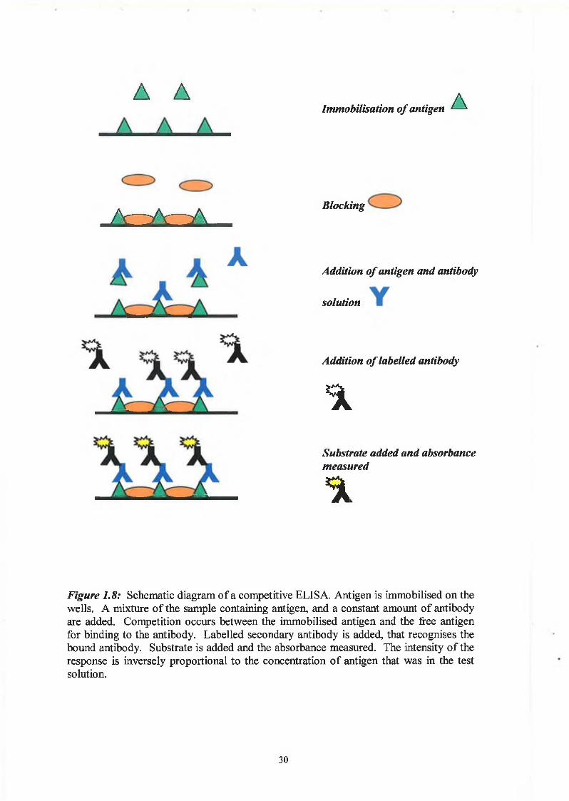
Figure 1.8. Antigen is immobilised, and a mixture of antibody and free antigen are

added. The amount of free antibody available to bind to the immobilised antigen is

inversely proportional to the amount of free antigen in the solution. The subsequent

substrate colour change is inversely proportional to the antigen in the solution. An

example of a variation of the competitive assay is the inhibition assay. This is the

immobilisation of antigen, followed by the addition of a sample of antigen free in

solution, followed by addition of antibody. During the incubation period, competition

occurs between the immobilised antigen and the antigen free in solution for binding by

the antibody. This step is then followed by incubation with anti-species antibody

that is enzyme-labelled. The resulting change in substrate colour in the final step is

inversely proportional to the amount of free antigen in the test solution. The difference

between the inhibition assay and the competitive assay is subtle. In the inhibition assay,

the antigen and antibody are not equilibrated before each are added to the antigen-

coated wells.

1.6.1.2 Non-Competitive Immunoassay

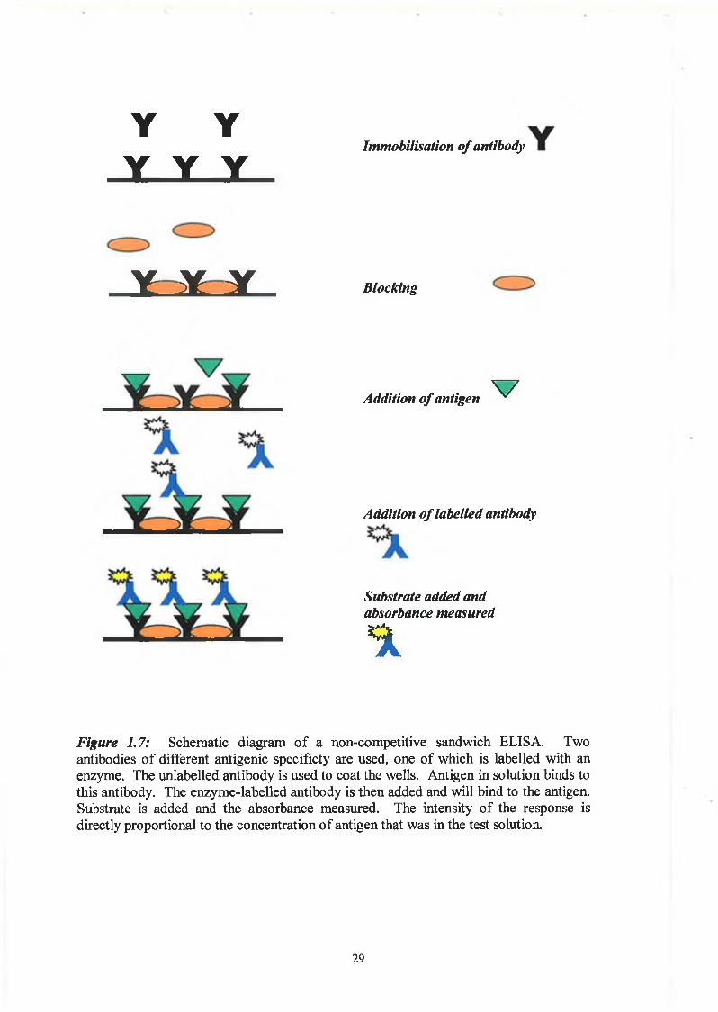
In a sandwich ELISA, (Figure 1.7), two different antibodies, reactive with different

epitopes of the antigen are required. One antibody is immobilised to the solid phase,

and the antigen is then added. This is followed by the addition of another antibody that

is specific for a different epitope of the antigen.

One of the most common rapid assays available currently are the dip-stick or test strip

immunoassays. These involve antibodies being coated on surfaces such as nitrocellulose

strips. Test strip assays usually employ a sandwich or competitive immunoassay format

and lateral flow of the applied sample facilitates accumulation at a region pre-coated

with antigen, (Figure 1.9). An example of a format used is the One-Step Rapid Opiates

Test, (Craig Medical, USA), for detection of opiates in urine. The urine sample is

applied to the chromatographic strip and reacts with labeled antibody-dye conjugate.

They laterally flow along the strip and any unbound antibody-dye conjugate binds to

immobilised antigen conjugate in the test zone of the strip. This produces a specific

27

colour line in the result window of the strip, which indicates a negative result. On the

other hand, if the urine contains opiates, at a concetration above the cut-off level, the

antibody-dye conjugate binds to the free drug in the urine and forms an antigen-

antibody-dye complex. This complex competes with the immobilised antigen conjugate

in the test zone, preventing the development of a coloured line. A positive control is

built in by incorporating a non-specific sandwich dye conjugate reaction.

2 8

Y YY Y Y

Immobilisation o f antibody

Y Y Y Blocking

Addition o f antigen V

Addition o f labelled antibody

Substrate added and absorbance measured

%

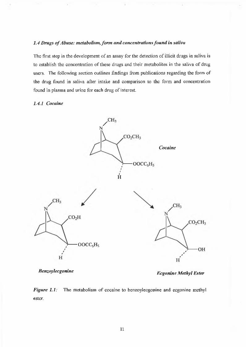
Figure 1.7: Schematic diagram of a non-competitive sandwich ELISA. Twoantibodies of different antigenic specificty are used, one of which is labelled with an enzyme. The unlabelled antibody is used to coat the wells. Antigen in solution binds to this antibody. The enzyme-labelled antibody is then added and will bind to the antigen. Substrate is added and the absorbance measured. The intensity of the response is directly proportional to the concentration of antigen that was in the test solution.

29

(i) Negative Result

(ii) Positive Result

(iii) Invalid Result

Test Line Control Line Absent

Figure 1.9: Diagram of example of lateral flow 'dip stick'-type immunoassay for the detection of drugs in a urine sample. The development of the two lines, a test line and a control line, indicates a negative test for the targeted drug (i). The development of the control line and absence of the test line indicates a positive result (ii). The absence of a control line in the window indicates an invalid result regardless of the test line result (iii).

31

A AImmobilisation o f antigen A i

/v-w-w Blockingins

Addition o f antigen and antibody

solution

Addition o f labelled antibody

%

Substrate added and absorbance measured

%

Figure 1.8: Schematic diagram of a competitive ELISA. Antigen is immobilised on the wells. A mixture of the sample containing antigen, and a constant amount of antibody are added. Competition occurs between the immobilised antigen and the free antigen for binding to the antibody. Labelled secondary antibody is added, that recognises the bound antibody. Substrate is added and the absorbance measured. The intensity of the response is inversely proportional to the concentration of antigen that was in the test solution.

30

1.6.2 Enzyme-Multiplied Immunoassay Technique

EMIT is an homogenous competitive assay. The antigen is labelled with an enzyme

and mixed with the sample antigen free in solution and antibodies. Competitive binding

takes place, and the binding of the enzyme-labelled antigen, sterically hinders the active

site of the enzyme thereby preventing enzyme activity. When unlabelled free antigen is

added, it competes with the labelled antigen for binding to the antibody. The greater the

level of antigen added, the greater the level of unbound enzyme-labelled antigen

resulting in greater enzyme activity. Behring Diagnostics Inc supply a number of EMIT

kits for the detection of cannabinoids, opiates, cocaine and amphetamine.

1.6.3 Fluorescence Polarisation Immunoassay

FPIA is a homogenous competitive assay in which a known amount of antigen or drug

analog is labelled with fluorescein and mixed with sample antigen and antibody in free

solution. The labelled and sample antigen compete for binding to the antibodies and

detection is by means of a vertically polarised detector. The detection is based on the

difference in the rotation speeds of the free and bound fluorescein-antigen. The free

fluorescein-antigen rotates at higher speeds and results in emission of light in a different

plane to the incident light, so it will not be detected. The bound fluorescein is not free

to rotate and so the emitted light is almost in the same plane as the incident light and so

it is picked up. A major advantage of the FPIA is that it is homogenous and there is no

need for the immobilisation step.

1.6.4 Detection o f analytes by immunoassay using up-converting phosphor

technology.

Up-converting phosphor technology is based on lanthanide-containing, ceramic

particles that can absorb infrared light and emit visible light. The important distinction

between fluorescence and phosphorescent is that biological matrices do not up-convert

and so there is no background sample autofluorescence. Niedbala et al. (2001 A) have

developed lateral flow immunoassay strips for the detection of drugs of abuse using this

up-converting phosphor technology, (UPT). The assay strips are designed like a lateral

32

flow test that uses colloidal gold or latex particles. The up-converting phosphor

particles, about 400nm in diameter, are covalently conjugated to the antibodies using

EDC/NHS chemistry. The basis of the test is that in the competitive format used, the

UPT-antibody-drug complex will not bind to the test line, immobilised drug-protein

conjugate, in the presence of drug in the sample. If the drug is not present in the

sample, the UPT-antibody binds to the immobilised drug-protein on the test line giving

a signal. This response at the test line is inversely proportional to the amount of drug in

the sample.

1.6.5 Agglutination

Agglutination assays are common, and easy to perform. The basis of the assay is the

specific mixture of antibody and antigen and visible aggregation of particles. They are

homogenous, as they do not require the separation of free and antibody-bound fractions

of the analyte. A variation of the agglutination assays include haemagglutination and

haemagglutination-inhibition. In the case of haemagglutination the antigen-antibody

interaction is mediated using red blood cells pre-coated with the antigen of interest. The

addition of test sample containing antibodies results in a visual agglutination,

(Fitzpatrick et al, 2000). Latex agglutination is similar to haemagglutination assay, in

this case the antigen or antibody is coated to latex beads. An example of one popular

commercially available agglutination test for drugs of abuse in urine, is the Ontrak®

kits, by Roche Diagnostics.

1.6.6 Biosensors

One description of a biosensor is as follows: a sensing device that incorporates a

biological entity as a fundamental part of the sensing process (Diamond, 1998).

Biosensors have been applied to the field of detection of drugs of abuse, e.g., Ogert et

al. (1992), developed a continuous flow immunosensor for the detection of cocaine

based on a fluorescence assay. The immunosensor is based on the displacement of the

fluorophore-labeled cocaine from immobilised antibody. It consists of a sepharose

microcolumn with immobilised anti-cocaine antibodies. A buffer flows into the column

and exits to an on-line fluorimeter. The immunosensor depends on the immobilised

antibodies for specific recognition of cocaine and its closely related metabolites. The

33

displacement of fluorophore-labelled benzoylecgonine from the immobilised antibodies

by samples containing cocaine produces the fluorescent signal. The limit of detection

of cocaine was 5ng/ml.

Devine et al. (1995) developed a fibre optic biosensor for the detection of cocaine.

Anti-benzoylecgonine monoclonal antibodies were immobilised onto quartz fibres and a

flow fluorometer was used to detect changes in the fluorescence. A BEC-fluorescein

conjugate was produced, and it bound to the immobilised antibody. The cocaine in the

test sample competed for binding to the antibody in a concentration-dependant manner,

and so reduced the initial rate or steady state fluorescence. The regenerable nature of

this assay and that described by Ogert et al. (1992), is key to its success. The detection

limit for cocaine in this assay was 5ng/ml and for benzoylecgonine was 30ng/ml. Yu et

al. (1996) presented results from a similar flow immunosensor for the detection of

benzoylecgonine in urine samples, giving a 97% correlation with results from samples

analysed by GC-MS.

Another variation on the theme of fluoroimmunoassay-based biosensors is described by

O’Connell et al., (1999). They evaluated a fluoroimmunoassay using microbeads

instead of quartz fibers as a solid support, and the commercial system KinExA™

(Kinetic Exclusion assay) for the bead handling flow fluorometer system. A quantity of

beads are coated with antibody and are introduced into a capillary flow cell and retained

on a screen. Free benzoylecgonine in the test solution competes with fluorescein-

benzoylecgonine conjugate for binding to the screen, and so the bead-bound

fluorescence is reduced in the competitive format. The system monitors the binding of

the fluorescent conjugate to the fiber in real-time and so it is also designed to measure

association and dissociation rate constants of antigen-antibody complexes, similar to

surface plasmon resonance technology.

Analyte 2000 (Research International, Woodinville, WA USA) is a fibre optic

biosensor that has been applied to the analysis of cocaine and its metabolites in human

urine using a competitive fluorescence immunoassay, (Nath et al., 1999). In this case,

the binding of anti-benzoylecgonine monoclonal antibody to casein-benzoylecgonine

antigen-coated optical fibres was inhibited by the presence of cocaine. The bound

antibody, which is inversely correlated to the cocaine concentration in the sample, is

measured by the fluorescence produced by the subsequent binding of cyanine dye-

tagged anti-mouse antibody. The use of evanescent excitation of fluorescence in fibre

34

optic biosensors ensures that only fluorophore bound to the surface of the fibre optic is

detected, and so the sensor does not detect any sample constituents or unbound

fluorophores. The minimum level of detection in this assay was 0.75ng/ml. The

Analyte 2000 is composed of four single-fibre optics and so can perform the analysis of

four drugs in the one sample. Currently, the main disadvantages with the systems is the

lack of automation and the labour intensive preparation of the fibres. These problems

however, are likely to be addressed and improved upon as further applications are

developed. For all of the types of immunoassays described it must be reiterated, that

their performance in terms of sensitivity and specificity are fundamentally associated

with the quality of the antibodies that are used.

As mentioned previously, the detection of drugs by chromatographic methods requires

an extraction step, as opposed to immunoassays that usually do not require a sample

pretreatment step. There has been considerable research into amperometric and

piezoelectric immunosensors (Cassidy, 1998), however, they do not seem to have found

a place yet in the routine analytical laboratory.

Surface plasmon resonance-based biosensors are very successful analytical tools and are

being used increasingly in research and anlytical labs. They are discussed in Chapter 5,

in detail.

A novel, non-immunological-based biosensor using frog melanphores to detect opioids

has been developed by Karlsson et al. (2002). This sensor harnessed the ability of

lower vertebrates such as fish and frogs to change colour. In response to specific

stimulii, chromaphores change colour by redistributing their pigment granules within

the cell. Melanophores which are a particular type of chromophore that contains brown

melanin pigment granules, were transfected with human opiod receptor 3 and cultured

and used for opiate detection. In the presence of opiods, the pigment granules

aggregated in a dose-dependant response in the melanophores. This technique of

transfection of melanophores with different receptors may create an alternative

biosensor for other substances. An example of another novel non-immunological-based

assay is the bioluminescent assay for heroin and morphine that uses heroin esterase and

morphine dehydrogenase linked to bacterial luciferase (Holt, 1996).

35

1.7 Commercial Tests

The ROSITA project, funded by the European Commission, produced comprehensive

papers on roadside drug testing in Europe. Work packages on different aspects of the

project include:

• Drugs and medicines that are suspected to have a detrimental impact on road user

performance, (Maes et al, 1999, www.rosita.org).

• Inventory of state-of-the-art roadside drug testing equipment, (Samyn et al., 1999).

• Operational, user and legal requirements across EU member states for roadside drug

testing equipment, (Moller et al., 1999, www.rosita.org).

• Evaluation of different roadside drug tests, (Verstraete & Puddu, 2000,

www.rosita.org).

• General conclusions and recommendations, (Verstraete & Puddu, 2000).

These informative documents can be accessed on the Rosita website at www.rosita.org.

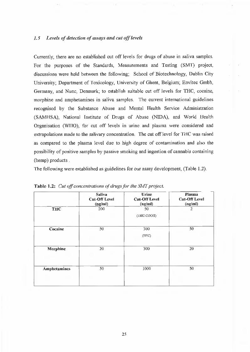
There are numerous commercial kits available for the screening of urine for drugs of

abuse. However, because of the different form and concentrations of the drugs found in

saliva, they are not ideally suited to saliva screening, and are not marketed for such an

application. Three devices are commercially available for the purposes of roadside drug

testing in saliva samples. These are Drugwipe (Securetec GmbH, Germany), Oral

Screen (Avitar Technologies Inc, USA), and Rapiscan, (Cozart Biosciences Ltd., UK).

The advantages and disadvantages of each are detailed in the above reports. Drugwipe

is used for the detection of drugs on surfaces. Different tastes are available for the

detection of opiates, cocaine, cannabis and amphetamines. The test is a lateral flow

memebrane immunoassay, that consists of a wiping section and the chromatographic

reaction cartridge. The substances captured on the wiping device are applied to the

strip. The addition of water allows the progression of the immunnoassay, (Securetec,

Germany). Drugwipe, as reported by the Rosita project, is available for the detection of

recent use of cocaine, amphetamine, and designer amphetamines. They found that it

was unreliable for detection of cannabis and some false negative results with regard to

the detection of opiates. The Drugwipe for opiates is supposed to give a positive test

with 5ng/ml of heroin, morphine or codeine. Kintz (1998), found an unacceptable

number of false negative results in a study in which volunteers were administered

codeine and subsequently tested using Drugwipe and saliva samples were also analysed

36

http://www.rosita.org




by GC-MS. Part of the problem contributing to the false negatives may have been the

inadequate sample collection or too low a cut-off mark for the analyte. An advantage of

this test is that it does not involve saliva collection, instead, the tongue is wiped with a

device. This test has also been marketed for drug detection in sweat samples. Navarro

et al. (200IB) investigated the concentration of MDMA, in saliva with Drugwipe in a

controlled study where recreational users were administered MDMA in a double-blind,

cross-over, placebo clinical trial. Saliva samples were collected in addition to the ‘on

site’ procedure and these samples were retested in the lab using Drugwipe and also

tested using GC-MS. At 1.5 and 4 hours after administration, all eight subjects gave a

positive result. The cut-off level determined by comparison to the GC-MS results was

650ng/ml.

OralScreen is available for the detection of opiates, cocaine and cannabis,

(www.avitarinc.com). The ORALscreen System contains an oral fluid collection device,

and a test device containing a lateral flow membrane immunoassay. The main

disadvantage documented by the ROSITA project with this device, was the difficulties

with the saliva collection procedure. Many of the testers were in direct contact with the

saliva during the procedure. Barrett et al. (2001) of Avitar conducted a study

comparing the ORALscreen test for THC, cocaine, opiates and methamphetamine in

oral fluid with a laboratory-based urine screen that involved EMIT testing for THC,

cocaine metabolite, and opiates and by CEDI A® (Microgenics, USA) testing for

amphetamine and methamphetamine. CEDIA testing is a commercial immunoassay

that can be run on automated clinical chemical analyzers. The urine samples that tested

positive by these screening tests were then analysed by GC-MS confirmation assays.

The results show very good correlation for detection of cocaine and opiates for 2.5 and

3 days after use, respectively. THC was detected by the ORALscreen on the day of use

and one day following use. There was good correlation between the urine and oral fluid

testing for methamphetamine. However the number of days following use was not

determined.

Rapiscan, produced by Cozart Bioscience, is probably the most advanced roadside

testing device as it incorporates a digital read-out of the results. It has been tested in a

major trial by UK authorities. The test consists of three components, a test swab, for

saliva collection, a disposable cartridge, and an instrument which displays the results.

The sample is placed in the cartridge in the hand held device and the immunochemical

37

http://www.avitarinc.com

reactions take place, giving results after five minutes, (www.cozart.co.uk). This test

detects cannabinoids, ecstasy, cocaine, opiates and benzodiazepines in a saliva sample

(Cozart Biosciences, 1999). The Rosita researchers described the device as

‘problematic’ during the course of their field test. The problems included insufficient

saliva collected, the test taking too long, and being too cumbersome. An advantage,

however, was the availability of the remainder of saliva that could be used for

laboratory confirmation. A recent paper by Jehanli et al. (2001), of Cozart

Biosciences, examined the results of a trials that involved testing saliva samples from

43 volunteers after consumption of codeine and cannabis. The results from the

Rapiscan device was compared with results obtained from immunoassays and GC/MS.

They found that positive opiates results were obtained for up to nine hours after

ingestion of the codeine, however, the cut-level for the cannabis test was too high at

lOng/ml THC, to detect marijuana use for more than a few hours after ingestion.

In the USA Intercept developed by OraSure Technologies, Inc, (Bethlehem, PA) is a

test kit in which the saliva is collected and then shipped to the designated lab for

analysis in an immunoassay format, (www.Orasure.com). Niedbala et al. (2001B & C)

have presented the results of the saliva analysis and corresponding urine analysis.

Using immunoassay cut-off values of lOng/ml and 2000ng/ml for positive opiate

presence in saliva and urine, respectively, it was found that the correlation was 93.6%.

In the corresponding test for marijuana, they found that the time course of the

concentration of THC in oral fluid is similar to that described for THC in plasma. This

is remarkable as the presence of THC in saliva is believed to be as a consequence of

impregnation, rather than diffusion of the THC from the plasma. Concentration of THC

in the oral fluid declined in a multi-phasic nature that suggests the presence of fast and

slow releases of sequestered THC in the oral cavity. The concentrations of the THC

detected in the oral fluid were higher in the first six hours after smoking and the

concentration in urine increased and exceeded the urine concentration after about 16

hours.

Immunological tests for drugs of abuse in urine are based on the following techniques:

enzyme multiplied immunoassay technique (EMIT) such as EMIT® d.a.u.™ (Syva,

UK), agglutination, such as Ontrak®, (Roche Diagnostics), fluorescence polarisation

immunoassay, TDx® (Abbott Diagnostics) and radioimmunoassay, Abuscreen®

(Roche Diagnostics). There are many different tests available for urine testing and

these are also documented in the ROSITA reports. These urine screening tests are in

38

http://www.cozart.co.uk

http://www.Orasure.com

widespread use in analytical labs in institutions, hospitals, and clinics and are of an

overall good standard. The limitations of the urine tests are that they can only be used

for detection of drug metabolites in urine. The form of ding metabolites found in urine

can differ significantly from the drug form found in saliva. Another significant

limitation is that the cut off level of these tests (Table 1.2) is generally greater than the

cut off level that would be acceptable for saliva testing. This therefore limits the use of

these tests to urine screening for drugs of abuse.

39

1.8 Summary o f Introduction

Assays for the detection of drugs of abuse range in complexity from immunoassays to

more complicated analytical methods such as gas chromatography/mass spectroscopy

(GC/MS). The development of immunoassays for the detection of illicit drug use that

could be used in roadside testing would mean that screening could be performed in the

same manner as current alcohol testing and the confirmatory test would be by GC/MS.

Currently, the most popular biological media for quantitative measurement of illicit

drugs is plasma and urine. However, saliva is now becoming common because of the

obvious advantage of the non-invasive nature of collection and the correlation between

psychological impairment and the level of detection of the illicit drugs and metabolites.

In the development of the rapid roadside tests, the following considerations should be

taken into account. The test must be:

• rapid

• specific and sensitive, with positive results correlating to the legal cut off level as

determined by authorities such as the National Institute of Drugs of Abuse (N1DA)

• degree of cross reactivity with drug metabolites and other common legal substance

needs to be established

• ‘user-friendly’ as it will be performed by non-lab personnel

The international scientific and legal communities must also begin to create guidelines

for the establishment of such tests in order that all the essential qualities can be

incorporated by research and development groups.

40

1.9 Aims o f Thesis

There is a huge demand in the scientific and security communities to establish rapid,

robust, specific, sensitive assays for the detection of drugs of abuse in saliva samples.

The aim of this project is the development of novel assays for the detection of drugs of

abuse in saliva.

Chapter 3 describes the process of producing morphine and cocaine protein conjugates

for the immunisation procedures. The drug-protein conjugates were used for the

production of polyclonal antibodies to morphine and cocaine. THC-BSA was also used

for the production of anti-THC polyclonal antibodies. The purified antibodies were

then applied to an ELISA format for the detection of morphine, cocaine and THC.

Chapter 4 describes the production, purification and characterisation of the anti

amphetamine and anti-methamphetamine monoclonal antibodies. Successful clones of

each antibody were produced and the antibodies were applied to an ELISA for the

detection of amphetamine, methamphetamine, and the other common designer

derivatives, MDA, MDMA, MDEA, MBDB. The ELISA was also established using

saliva samples as the matrix. Particular attention was given to the cross reactivity

studies of these antibodies during the cloning procedure, as many other legal

‘amphetamine like’ molecules, such as, ephedrine have shown cross reactivity with

assays reported in the literature.

Chapter 5 expands the characterisation and application of the anti-amphetamine and

anti-methamphetamine monoclonal antibodies using biosensor technology (BIAcore).

Affinity constant measurements were determined using two different techniques, the

classic ELISA based Friguet method and the solution-phase BIAcore assay. The

antibodies were also applied for the development of a BIAcore-based inhibition assay

for the detection of amphetamine and methamphetamine in saliva samples.

Chapter 6 describes the results of a pilot clinical study that was conducted to investigate

the application of the antibodies produced for the detection of drugs of abuse. A

number of different assays were used for the analysis of THC, and morphine. A

41

prototype of the Envilec device was used, and a rapid test for THC using the anti-THC

polyclonal antibody was developed. BIAcore assays were also investigated for the

detection of morphine in saliva samples. Real saliva sample samples were collected

from drug users and analysed in the different formats. Specific issues relating to the

stability of drugs in biological samples and the collection and storage of real saliva

samples are also discussed.

42

Chapter 2

Materials and Methods

43

2.1 Materials

All chemicals and materials were obtained from Sigma Chemical Co. (Tallaght, Dublin

24). The exceptions are listed in Table 2.1.

Table 2.T. Chemicals that were obtained from companies other than Sigma-Aldrich.

Non-Essential Amino Acids Gibco BRL

Fetal Calf Serum Gibco BRL

Sodium Pyruvate Gibco BRL

Briclone (Bioresearch Ireland) Archport

Hydrochloric Acid (HC1) (Riedel de Haen) Riedel de Haen

Acetic Acid Riedel de Haen

Tween 20 Riedel de Haen

PBS Tablets Oxoid

THC-BSA Fitzgerald Industries

Morphine-BSA Fitzgerald Industries

BEC-BSA Fitzgerald Industries

BEC-BgG Fitzgerald Industries

Amphetamine-BSA Fitzgerald Industries

Methamphetamine-B S A Fitzgerald Industries

THC-HRP Fitzgerald Industries

Cocaine McFarland Smith

Morphine McFarland Smith

CM-Dextran Fluka Chemicals

Bicinchoninic Acid Assay Kit Pierce and Warriner

All licences necessary for importing and possessing illicit drugs were obtained.

44

Full Addresses of Suppliers

Archport, Dublin City University Campus, Dublin 9.

Fitzgerald Industries, 34 Junction Square Drive, Concord, MA 01742, USA.

Fluka Chemicals, Gillingham, Dorset, UK,

Gibco BRL, RenfewRd., Paisley, PA4 9RF, Scotland.

McFarland Smith, Wheatfield Road, Edinburgh, EH11 2QA, Scotland.

Oxoid, Basingstoke, Hampshire, RG24 8PW, UK.

Pierce and Warriner, Chester, UK.

Riedel de Haen, Wunstorfer Strabe, D-3106, Seelze, Hanover, Germany.

Sigma Aldrich, Tallaght, Dublin 24.

45

Table 2.2\ Equipment used and the supplier.

2.2 Equipment

Equipment Supplier

BIAcore 3000 BIAcore AB

3015 pH Meter Jenway Ltd.

Titertek Multiscan Plate Reader Medical Supply Company

Millipore Filtration Device Medical Supply Company

Heraeus Labofuge 6000 Heraeus Instruments

Biofuge A Microcentrifuge Heraeus Instruments

Ultrafiltration Cell Amicon

Heraeus C02 Incubator EG 115IR Heraeus Instruments

Holten 2448K Laminar Flow Unit Holten Laminar A/S

Nikon Diaphot Inverted Microscope Nikon

UV 160A Spectrophotometer Shimadzu

RM6 Lauda Waterbath AGB Scientific

SB1 Blood Tube Rotator Medical Supply Company

Atto dual minislab system AE-6450 Atto


AGB Scientific, Dublin Industrial Estate, Glasnevin, Dublin 9.

Amicon Inc., Beverely, MA 01915,

Atto, Bunhyo-Kui, Tokyo 113, Japan.

BIAcore AB, Uppsala, Sweden.

Holten Laminar A/S, Gydevang 17, DK 3450 Allerod, Denmark.

Heraeus Instruments Inc., 111-a Corporate Boulevard, South Plainfield, NJ 07080.

Jenway Ltd., Gransmore Green, Felsted Dunmow, Essex, CM6 3LB, UK.

Medical Supply Company, Damastown, Mulhuddart, Dublin 15.

Nikon Corp., 2-3 Marunouchi 3-Chrome, Chiyoda-Ku, Tokyo, Japan.

Shimadzu Corp., 1 Nishinokyo-Kuwabaracho, Nakagyo-ku, Kyoto 604, Japan.

46

2.3 Consumables

Table 2.3\ Consumables used and the suppliers.

Consumable Source

BIAcore sensor chips BIAcore

Plastic labware, e.g., eppendorfs,

centrifuge tubes, pipettes, pipette tips

Sarstedt

Maxisorb 96 well plates Nunc

Tissue culture plasticware Nunc

Ultrafiltration filters Amicon

Saliva Collection Device Trinity Biotech


Amicon, Beverely, MA 01915.

BIAcore AB, Uppsala, Sweden.

Nunc, Kamstrup DK, Roskilde, Denmark.

Trinity Biotech, Southern Cross Business Park, Bray, Co. Wicklow.

Sarstedt, Sinnottstown Lane, Drinagh, Co. Wexford.

47

2.4 Standard Solutions

Phosphate Buffered Saline (PBS)

One PBS tablet was dissolved in lOOmls deionised water per the manufacturers

instructions. The final solution contains lOmM phosphate buffer with 0.14 M NaCl, pH

7.2-7.4.

PBS/Tween

PBS containing 0.05% (v/v) Tween-20

Hepes Buffered Saline (HBS)

50 mMNaCl, 10 mM Hepes, 3.4 mM EDTA, and 0.05% (v/v) Tween-20. The pH was

adjusted to pH 7.4 with 2M NaOH. The solution was filtered through a 0.2p.m filter and

degassed.

2.4.1 Cell culture media

DM KM

DMEM (Dulbecco’s modification of Eagle’s medium) supplemented with 2mM L-

glutamine, 25(ig/ml gentamicin and 10% (v/v) fetal calf serum.

HAT

DMEM (as above) supplemented with non-essential amino acids, ImM sodium

pyruvate, lOOuM hypoxanthine, 400nM aminopterin, and 16uM thymidine.

HT prepared as for HAT without aminopterin.

48

2.4.2 SDS PA GE Solutions

Stock Solutions

• 30% (w/v) acrylamide containing 0.8% (w/v) bis-acrylamide

• 1.5 M Tris-HCl, pH 8 .8, containing 0.4% (w/v) SDS

• 0.5 M Tris-HCl, pH 6 .8, containing 0.4% (w/v) SDS

• 10 % (w/v) ammonium persulphate

Table 2.4: Volumes of stock solutions required for resolving and stacking gels for

SDS-PAGE.

Solution Resolving Gel

(10% (w/v) Acrylamide)

Stacking Gel

(3% (w/v) Acrylamide)

Distilled H20 14.0 ml 5.625 ml

30% (w/v) Acrylamide 10.5 ml 1.875 ml

1.5 M Tris pH 8.8 6.3 ml -

0.5 M Tris pH 6.8 - 0.9 ml

10% (w/v) SDS 0.18 ml 0.075 ml

TEMED 0.03 ml 0.075 ml

Ammonium Persulphate 0.15 ml 0.04 ml

Electrophoresis Buffer

25 mM Tris (pH 8.8), 192 mM glycine, and 0.1% (w/v) SDS.

Sample Loading Buffer

60 mM Tris (pH 6 .8), 25% (v/v) glycerol, 2% (w/v) SDS, 14.4 mM 2-mercaptoethanol,

and 0 .1 % (w/v) bromophenol blue.

Coomassie Blue Stain

Coomassie blue stain was prepared containing 0.2% (w/v) coomassie blue R250 in

30:10:60 (v/v/v) (methanol:acetic acid:water).

49

Destain Solution

Destain was made up with methanol:acetic acid:water in a 10:7:53 (v/v/v) ratio.

2.5 Production o f drug-protein conjugates

2.5.1 Conjugation o f morphine-3-glucuronide to protein

Morphine-3-glucuronide (25mgs) was dissolved in 0.5mls 0.15M HC1 and the solution

made up to 2.5mls in 0.05M phosphate buffer, pH 7.8. Solid NHS was added to the

morphine-3-glucuronide to give a final molarity of 0 .1M. EDC was dissolved in

1.25mls H2O and added to the mixture to give a final molarity of 0.4M. The solution

was mixed for 10 minutes with stirring. Protein (OVA, BSA, or BTG) (30mgs) was

dissolved in 2.5mls 0.05M phosphate buffer, pH 7.8. This was added to the mixture and

stirred for 1-2 hours at room temperature. The mixture was dialysed extensively against

PBS at 4°C overnight.

2.5.2 Conjugation o f cocaine to protein

A solution of cocaine was prepared in phosphate buffered solution as the phosphate ions

could serve as a catalyst for the hydrolysis reaction, (Das Gupta, 1982). A 5mg/ml

solution in PBS was prepared and stored at room temperature for one week to allow the

conversion of cocaine to BEC. NHS was added to 1 ml of the solution to give a final

molarity of 0.1M. EDC was dissolved in 0.25mls H2O and when added to the mixture

gave a final molarity of 0.4M The solution was mixed for 10 minutes at room

temperature. lOmgs of protein (OVA, BSA or BTG) was dissolved in 0.5mls 0.05M

phosphate buffer, pH 7.8. This was added to the mixture and stirred for 1-2 hours at

room temperature. The mixture was dialysed extensively against PBS at 4°C overnight.

50

2.5.3 Commercial conjugates

Morphine-bovine serum albumin (morphine-BSA) conjugate was obtained from

Fitzgerald Industries International, MA, USA. The morphine was conjugated to the

BSA at the -3 position. The molar ratio of morphine to BSA of the conjugate was

123:1.

Benzoylecgonine-bovine serum albumin (BEC-BSA) was obtained from Fitzgerald

Industries International, M A USA. The molar ratio of BEC to BSA of the conjugate

was 60:1.

Tetrahydrocannabinol-bovine thyroglobulin (THC-BTG) was obtained from Fitzgerald

Industries International, MA, USA. The THC was conjugated through the delta-8

position.

2.6 Immunisations fo r polyclonal and monoclonal antibody production

The following protocols are employed for the production of polyclonal and monoclonal

antibodies. Three rabbits were immunised with THC-BTG, BEC-BSA and morphine-

BSA. Two groups of mice (4 in each group) were immunised with amphetamine-BSA

and methamphetamine-BSA. Care of animals was in accordance with DCU guidelines.

All appropriate licenses were obtained and adhered to for work involving animals.

2.6.1 Immunisation Protocol fo r the production o f Monoclonal Antibodies

Animals Used

6 week old Balb/c female mice

Day 1:

Mice were immunized by sub-cutaneous injection with an emulsion (250ul)

consisting of a 1 mg/ml solution of hapten - protein conjugate mixed 1 : 1 with

Freund’s Complete Adjuvant

Day 21:

Re-immunized intraperitoneally

Note: Freund’s Incomplete Adjuvant is used instead of Freund's Adjuvant.

51

Day 28:

A blood sample was collected (by least invasive method - tail bleed) and the

antibody titre determined by ELISA against the respective antigen.

Day 52:

The mouse was boosted intraperitoneally using Freund’s Incomplete Adjuvant.

Antiserum Recovery:

Animal was re-immunised and serum titred, when possible, until an acceptable

titre was obtained and a schedule of immunisations of approximately six

months or greater is completed.

Five days after the last immunisation, the animal was sacrificed and the blood

and the spleen removed.

2.6.2 Immunisation Protocol fo r the production o f Polyclonal Antibodies

Animals Used

Adult New Zealand white female rabbits

Day 1:

Rabbit immunised by sub-cutaneous injection with an emulsion (1ml)

consisting of a 1 mg/ml solution of hapten - protein conjugate mixed 1 : 1 with

Freund’s Complete Adjuvant.

Day 14:

Rabbit re-immunised as before.

Note: Freund’s Incomplete Adjuvant was used instead of Freund’s Complete

Adjuvant.

Day 28:

5ml blood sample removed from ear vein and the antibody titre determined

against the respective antigen.

Day 35:

Rabbits re-immunised as before.

Note: Freund’s Incomplete Adjuvant was used instead of Freund’s Complete

Adjuvant.

Day 42:

52

A blood sample was collected, as before, and antibody titre determined against

the respective antigen.

Antiserum recovery:

The animal was re- immunised and serum titred when possible, until an acceptable titre

(>1/500,000) was obtained and a schedule of approximately six months was completed.

At this point the animal was sacrificed and the blood recovered by cardiac puncture.

2.6.3 Preparation o f rabbit serum

For estimation of titre, the blood collected was allowed to clot for 2 hours at room

temperature. It was stored overnight at 4°C to allow the clot to tighten and then

centrifuged at 4,000 rpm for 20 minutes. The supernatant was removed and stored at -

20°C.

2.6.4 Preparation o f mouse serum

The procedure was as above with the exception of the centrifuge step; for mouse serum

because of the small volume, it was centrifuged at 13,000 rpm for 20 minutes.

2.7 Production o f monoclonal antibodies

All cell cultures were grown in an incubator with 5% CO2, at 37°C. Cell counts were

performed using a Neubauer Counting Chamber. The viability of cells was determined

by mixing the cells at a 5:1 ratio with 0.4% (w/v) Trypan Blue Solution. Dead cells

stained blue and viable cells remained white. The cells were visualised with a phase

contrast microscope. The count was performed within five minutes of mixing with the

Tryptan Blue.

2.7.1 Cell lines

Sp2/0 (ATCC CRL 1581) cell line was cultured in DMEM. The cells were subcultured

using a split ratio of 1:2 when the cells had grown to approximately 75% confluency.

53

2.7.2 Immunisation Schedule

The mice were immunised as per the schedule detailed in Section 2.6.1. Five days

before the fusion the mouse was re-immunised by an intraperitoneal injection of

0.25mls of 500|j,g/ml of drug-protein conjugate mixed 1:1 with Freund’s Incomplete

Adjuvant.

2.7.3 Fusion

Sp2/0

Sp2/0 cells were grown for at least two weeks prior to the fusion. The cells were grown

in T-75 flasks and on the day before the fusion they were subcultured at a split ratio of

1:2 as they should be in the logarithmic phase of growth for the fusion. On the day of

the fusion, the cells were centrifuged at 2000 rpm for 10 minutes and resuspended in

5mls of DMEM lacking FCS. They were counted, as described above, and stored until

needed.

Splenocytes

The immunised mouse was sacrificed and the spleen removed. The splenocytes were

harvested by injecting DMEM slowly into the spleen and repeating this procedure until

the spleen capsule is relatively clear. The splenocytes are then injected into a universal

centrifuge tube and a cell viability count performed separately. The cells were

centrifuged at 2000 rpm for 10 minutes and resuspended in 5mls of DMEM lacking

FCS.

The splenocytes and Sp2/0 cells were mixed to give a cell ratio of 10 splenocytes per

Sp2/0 cell. This cell mixture was pelleted and washed four times with 5mls of DMEM

lacking FCS.

All of the supernatant from the final wash was removed except for 50-100fil, and the

cells were resuspended by tapping. The suspension was placed in an ice/water bath and

1.5 mis of 50% (v/v) PEG was added to it over a one minute period, while the

suspension was swirled. The swirling was continued for a further 90 seconds. The

centrifuge tube was removed from the water bath and placed in the palm of the hand.

DMEM was pre-warmed to 37°C and 20mls was added to the suspension over a five

54

minute period, with constant slow swirling. The suspension was placed in a 37°C water

bath for 15 mins.

The mixture was centrifuged at 2000 rpm for 10 minutes and the cells resuspended at a

cell density of 1.2 x 106 cells/ml in HAT supplemented with 5% (v/v) Briclone. The

suspension was plated in 96 well cell culture plates at 0.1ml per well. The plates were

incubated for 7 days. On day 7, 50|il of HAT supplemented with 5% (v/v) Briclone

was added to each well. On day 8, 50fil of medium was removed and fresh medium

was added. This medium was then screened for antigen reactivity. Wells were fed as

required.

2.7.4 Screening o f hybridoma supernatants

Supernatants from the wells were screened for antigen reactivity using a conventional

ELISA format as described for the polyclonal antibody assays (Section 2.9). Positive

wells were scaled up to 48 well plates with 0.5mls medium. Wells subsequently found

to be positive were scaled up in 24, 12, and 6 well plates and finally in T-25 and T-75

flasks.

2.7.5 Storage o f cell lines

Cells were flushed off the surface of the tissue culture flasks using a pasteur pipette.

The media was centrifuged at 2000 rpm for 10 minutes. The resulting pellet was

resuspended in 2 mis of FCS and 2 mis of 10% (v/v) of DMSO in FCS. The mixture of

4mls was divided into four 1 ml cryovials. The freezing process was performed

gradually over a 2.5 hours time period using a freezing tray, in the vapour phase of

liquid nitrogen. The vials were then immersed in the liquid nitrogen and stored long

term.

2.7.6 Mycoplasma screening

Mycoplasma testing was performed through the services of the National Cell and Tissue

Culture Centre, Dublin City University. Cells were provided to them that had been

grown in antibiotic free medium for three sub-culturing processes.

55

2.8 Purification and Characterisation o f antibodies

2.8.1 Purification o f polyclonal rabbit serum

The rabbits were immunised as per the schedule detailed in Section 2.6. Fourteen days

pre-sacrifice, the rabbits were reimmunised by an intraperitoneal injection of 1 .0ml of

500|i,g/ml of drug-protein conjugate mixed 1:1 with Freund’s Incomplete Adjuvant. For

the production of anti-THC antibodies, THC-BTG was used as the immunogen and

THC-BSA was used as the screening conjugate. BEC-BSA was the immunogen and

BEC-BgG was used as the screening conjugate for the production of anti-cocaine

antibodies. Morphine-BSA was used as the immunogen and morphine-3-glucuronide-

OVA was the screening conjugate for the production of the anti-morphine antibodies.

2.8.1.1 Ammonium sulphate precipitation

A cold saturated ammonium sulphate solution was prepared and a volume added to an

equal volume of serum by dropwise addition, with constant stirring on ice. The mixture

was stirred on ice for one hour and then centrifuged at 3000 rpm for 20 minutes. The

supernatant was discarded and the pellet washed twice in lOmls of 45% (v/v)

ammonium sulphate. The final pellet was dissolved in 5ml of PBS and dialysed

overnight at 4°C against 5 litres PBS (pH 7.3, 0.15M NaCl).

2.8.2 Monoclonal Antibody Purification

2.8.2.1 Concentration o f tissue culture supernatant

The hybridoma cell line was grown for one to two weeks. The cell culture supernatant

was collected, and sodium azide was added at a concentration of 0.025% (w/v), final

concentration. The supernatant was stored at 4°C. 50ml of supernatant was

concentrated to 5 ml on a stirred ultracentrigfugation apparatus with a 76mm diaflo

ultrafilter membrane, with a molecular weight cut-off of 100 Kdaltons. The concentrate

was stored at 4 °C.

56

2.8.3 Protein G Affinity Column

A protein G column was prepared by adding 1 ml of protein G immobilised on

Sepharose 4B Fast Slow into a 5 ml syringe. The column was equilibrated with 20ml

PBS. The dialysate from the ammonium sulphate precipitation, in the case of

polyclonal antibody purification, and concentrated supernatant, in the case of

monoclonal antibody purification, was added to the column. 1ml of PBS was added to

the eluate and it was reapplied to the column. The eluate was collected and 4ml PBS

added and the mixture reapplied again. The collected eluate was applied to the column

again. The column was washed with 25ml PBS. The bound immunoglobulin was then

eluted by addition of 0.1M glycine/HCl, pH 2.5, to the column. The glycine was

equilibrated in the column for about 15 minutes. lOOul of Tris/HCl, pH 8.7 was added

to eppendorf collection tubes and the absorbance of the eluate was monitored in each at

280nm. The fractions containing protein were pooled and dialysed overnight at 4°C

against 5 litres of PBS with two changes of buffer.

2.8.4 Sodium Dodecyl Sulphate-Polyacrylamide Gel Electrophoresis

Sodium dodecyl sulphate polyacrylamide gel electrophoresis (SDS-PAGE) was

performed to assess the purity of the purified antibody fractions from the Protein G

purification step. The solutions used are outlined in Section 2.4.2. Samples were

prepared in sample buffer (4:1, sample :buffer ratio), and boiled for 5 minutes before

being loaded onto gels. The gels were run at 50 mA, using an ATTO verical minigel

electrophoresis system, until the blue dye of the sample buffer had reached the bottom

of the gel. The gels were subsequently stained for 30 minutes using Coomassie Blue

staining solution. The gels were destained by overnight incubation in destaining

solution.

2.8.5 Determination o f Protein Concentration - BCA

A Bicinchoninic Acid assay kit (BCA Kit, Pierce & Warriner, UK) was used for the

determination of protein content. Standard protein solutions were prepared in PBS

using either BSA or immunoglobulin. 10 pi of the solution was mixed with 190 pi of

57

BCA kit working solution in a 96 well plate. The plate was incubated at 37 °C for 30

minutes. The absorbance was read at 562 nm on the Titretek plate reader. A standard

curve of the protein standards was plotted and the concentration of the unknown

solutions was determined.

2.9 Immunoassays

2.9.1 Estimation o f rabbit antibody titre

Levels of antibody in serum from immunised rabbits were measured using ELISA. One

series of wells were coated with 10 0 [0.1 of the drug-protein conjugate (in the case of the

serum from the rabbit immunised with THC, 1 fig/ml of THC-BTG or THC-BSA was

used; for the serum from the rabbit immunised with BEC, 10 |_ig/ml BEC-BSA or BEC-

BgG was used; for the serum from the rabbit immunised with morphine-BSA 10 M-g/ml

morphine-3-glucuronide-OVA was used) and a second series of wells were coated with

the protein alone (BTG, BSA or OVA) at a concentration of 1 |ig/ml and incubated for

90 minutes at 37°C. The plates were washed five times in PBS/Tween and were

blocked by adding 200 fil of PBS/Tween containing 2% (w/v) milk powder and

incubated again for 90 minutes at 37°C. The serum was diluted in PBS/Tween and

PBS/Tween containing 0.1% (w/v) protein (BTG in the case of the THC-BTG

immunised rabbit, BSA in the case of the BEC-BSA and morphine-BSA immunised

rabbits), from 1/200 to 1/51,200. The plates were incubated for 90 minutes at 37°C.

The plates were washed five times with PBS/Tween. 100 (j.1 of commercial goat anti

rabbit lgG antibody, labeled with horseradish peroxidase at a dilution of 1/5,000 in

PBS/Tween, was then added to the wells. The plate was incubated for 90 minutes at

37°C. The plates were washed five times with PBS/Tween. The substrate for

horseradish peroxidase, OPD, was then added. The plates were incubated for 30

minutes in the dark at room temperature. The absorbance was read at 450 nm using a

microtitre plate reader.

58

2.9.2 Estimation o f mouse antibody titre

Levels of antibody in serum from immunised mice were measured using the above

procedure with the following exception: the secondary antibody used was

HRP-labelled rabbit anti-mouse IgG used at a dilution of 1/2000.

2.9.3 Non-Competitive Enzyme-linked Immunosorbent Assay fo r determination o f

antibody litre and optimal concentration o f protein conjugates

Microtitre plates were coated with a range of drug-protein concentrations by adding 100

pi of drug-protein conjugate dissolved in PBS (pH 7.3, 0.15M NaCl) to each well. The

plates were incubated for 60 minutes at 37°C. The plates were emptied and washed five

times with PBS/Tween (0.05% (v/v) Tween 20). The wells were blocked by addition of

100 pi PBS containing 2% (w/v) milk powder and incubated for 60 minutes at 37°C.

The plates were emptied and washed five times with PBS/Tween as before. Serial

dilutions of antibody in PBS (100 pi) were added into the wells of each conjugate

concentration on the plate. The plates were incubated for 60 minutes at 37°C. The plates

were washed five times with PBS/Tween as before. Enzyme-conjugated IgG (anti

rabbit in the case of polyclonals, and anti-mouse in the case of monoclonal antibodies)

were diluted in PBS/Tween containing 2% (w/v) milk powder (100 pi) was added to the

wells and incubated for 60 minutes at 37°C. The plates were washed five times with

PBS/Tween and 100 pi of substrate (OPD in case of HRP Conjugate, and p-NPP in case

of AP conjugate) was added to each well. The plate was covered with foil and left at

room temperature for 30 minutes for the colour to develop. The absorbance was

measured on a microtitre plate reader at 450nm.

2.9.4 Competitive Enzyme-linked Immunosorbent Assay

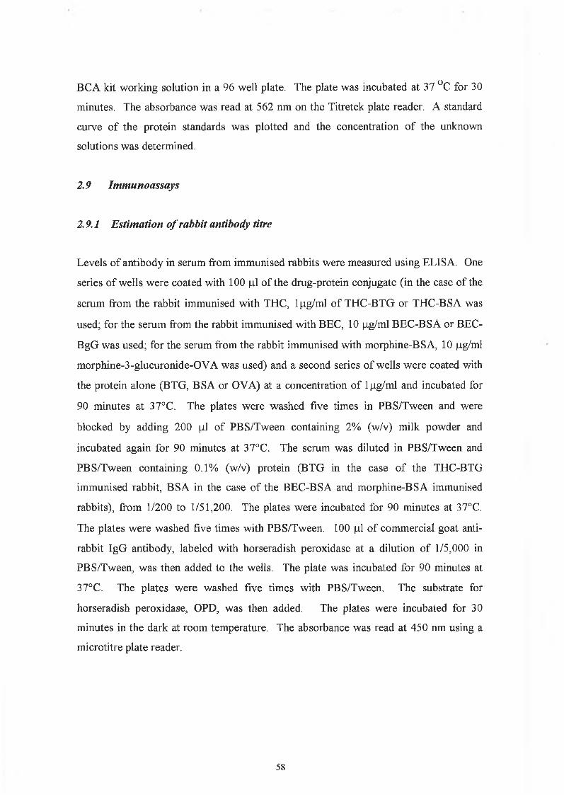
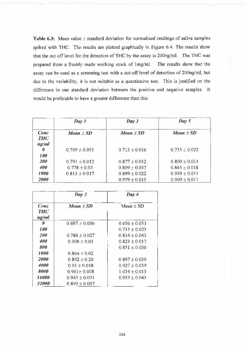
Microtitre plates were coated by adding 100 pi of drug-protein conjugate dissolved in

PBS (pH 7.3, 0.15M NaCl) to each well. The plates were incubated for 60 minutes at

37°C. The plates were emptied and washed five times with PBS/Tween (0.05% (v/v)

Tween 20). The wells were blocked by addition of 100 pi PBS containing 2% (w/v)

milk powder and incubated for 60 minutes at 37°C. The plates were emptied and

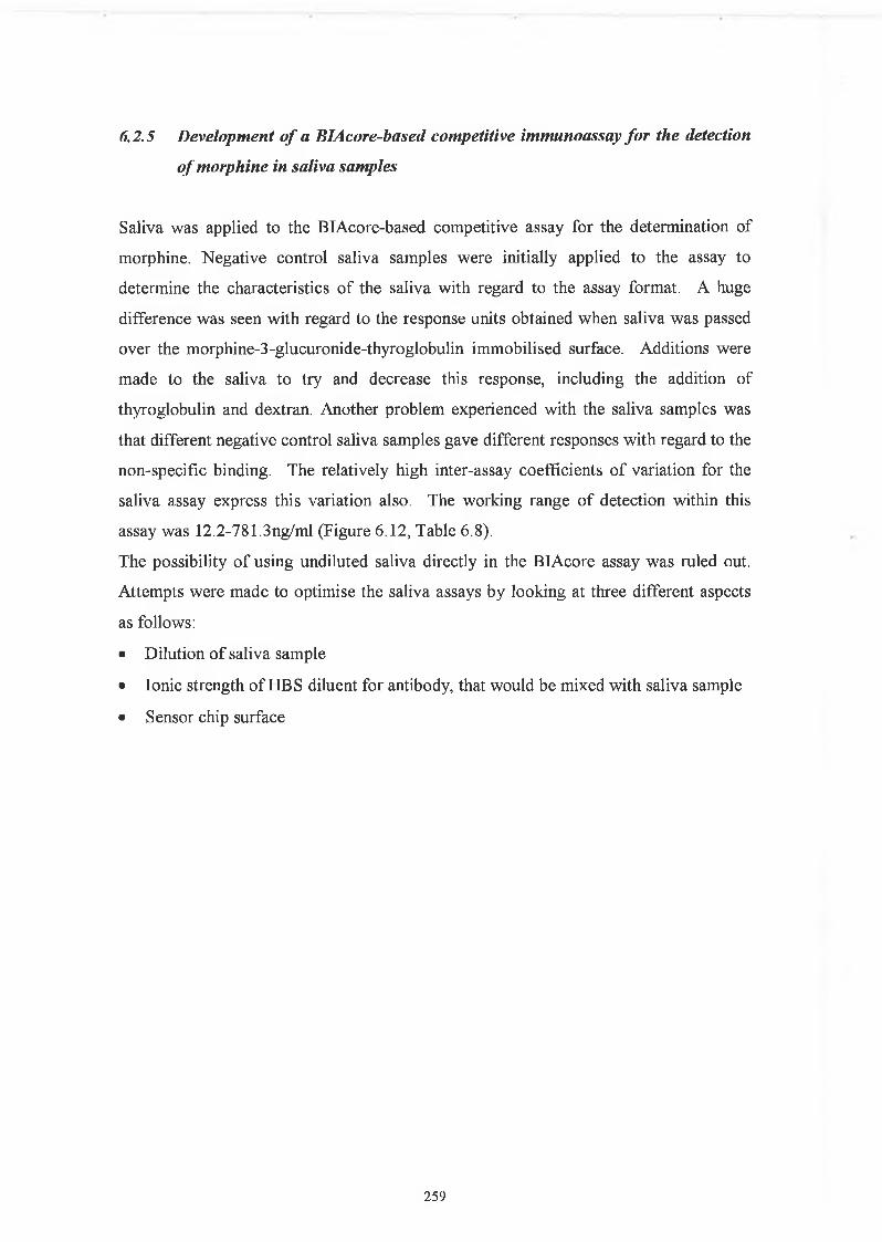
washed five times with PBS/Tween as before. Drug standard, 50 pi, containing from

59

0.38 ng/ml to 100,000 ng/ml and mouse anti-drug antibody, 50 pi, (diluted in

PBS/Tween containing 2% (w/v) milk powder) were added into each well. The plates

were incubated for 60 minutes at 37°C. The plates were washed five times with

PBS/Tween as before. Horseradish-peroxidase conjugated IgG was diluted 1/2000 in

PBS/Tween containing 2% (w/v) milk powder and 100 fj.1 was added to the wells and

incubated for 60 minutes at 37°C. The plates were washed five times with PBS/Tween

and 100 pi of substrate (0.4 mg/ml o-phenylenediamine (OPD), in phosphate citrate

buffer, pH 5, and 0.4 mg/ml of urea hydrogen peroxide) was added to each well. The

plate was covered with foil and left at room temperature for 30 minutes for the colour to

develop. The absorbance was measured at 450 nm on a microtitre plate reader. A

schematic representation of the ELISA procedure used is shown in Figure 2.1.

2.9.5 Isotyping o f monoclonal antibodies

ELISA plates were coated and blocked with the appropriate drug-protein conjugate and

milk protein, respectively, for 60 minutes, as described in Section 2.9.3. The

monoclonal antibody was added and incubated for 60 minutes. After washing, alkaline

phosphatase-labelled goat anti-mouse immunoglobulins were added to the wells and the

ELISA developed using para-nitrophenyl phosphate (p-Npp) provided in table form and

dissolved in the required volume of deionised H20, as described by the supplier’s

instructions. The absorbance of the reactive wells indicates the monoclonal antibody

isotype.

2.9.6 Affinity analysis ELISA - Friguet method

Twelve hours before the Friguet assay was performed, a series of antibody-antigen

mixtures were incubated in eppendorf tubes, to reach equilibrium. The solutions

contained a constant, nominal, dilution of antibody, refered to as ‘1 ’, and varying

concentrations of antigen. In another set of eppendorfs, serial dilutions of the nominal

concentration of antibody were prepared. These were used to construct the standard

curve of nominal antibody concentration versus absorbance at 450nm. Twelve hours

later, the ELISA was performed on these solutions, as per Section 2.9.3. Absorbance

readings at 450nm of the antigen:antibody mixtures were related to the nominal

concentration values by reference to the standard curve of nominal concentration versus

60

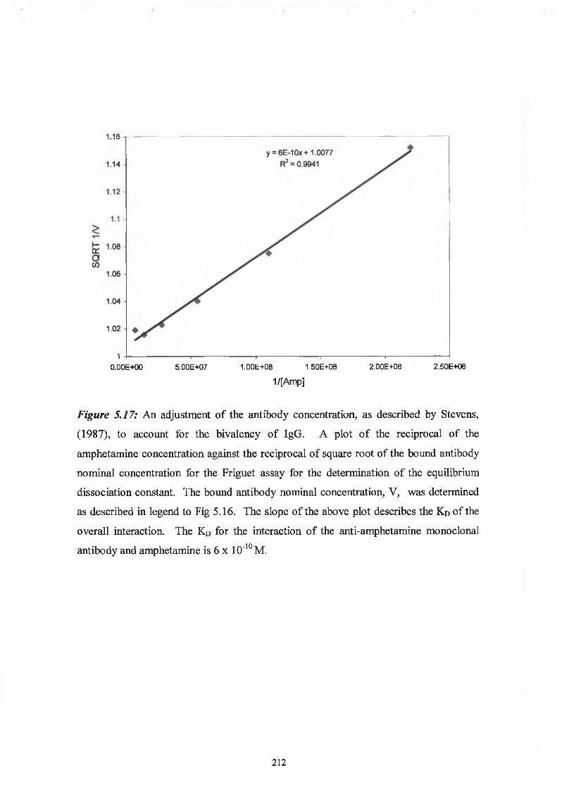
absorbance at 450nm. The fraction of total antibody bound by the antigen (v) was

calculated for each antigenrantibody mixture. The dissociation constant for the

antigen:antibody interaction was defined by the slope of the plot of 1/v versus 1 /[A],

(see Section 5.1.5).

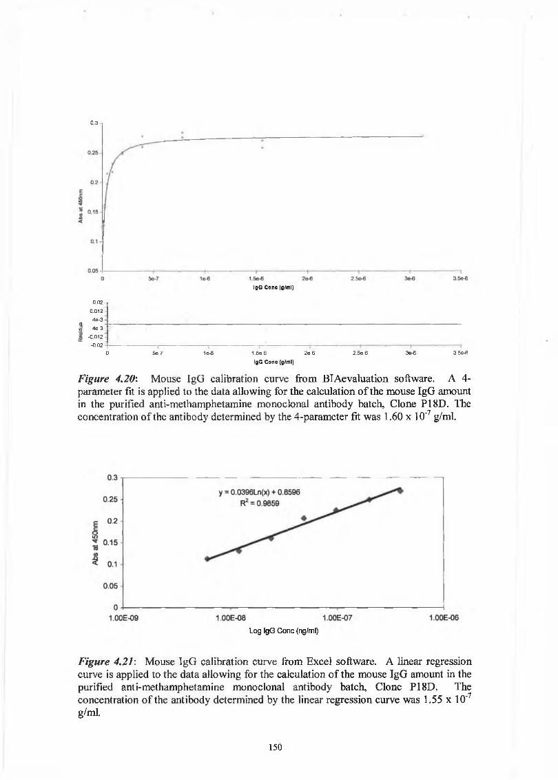
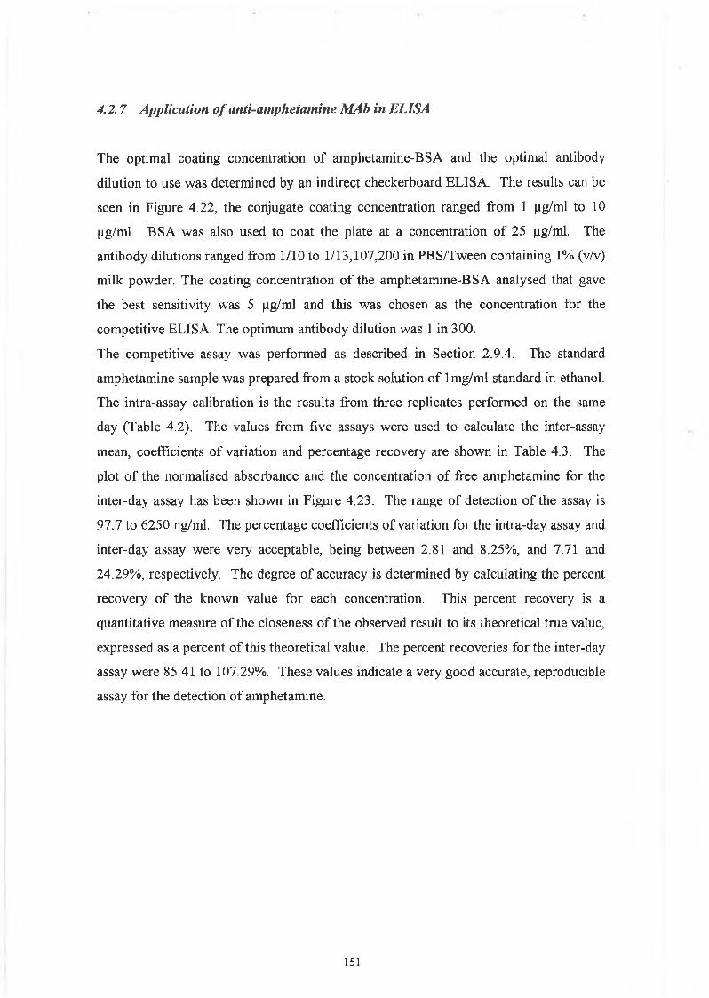
2.9.7 Determination o f immunoglobulin concentrations by affinity capture ELISA

Commercial goat anti-mouse immunoglobulin at a concentration of 10 (J.g/ml was used

to coat the wells of a microtitre plate, and it was subsequently blocked with PBS

containing 2% (w/v) milk powder as described in Section 2.9.3. Dilutions of mouse

IgG of known concentration were prepared in PBS. Dilutions of the purified antibody

were also prepared in PBS. 100 (ill of the solutions (standards and unknowns) were

added to the wells and the ELISA developed as described in Section 2.9.3. A standard

curve of absorbance at 450nm versus mouse IgG concentration was used for the

determination of the mouse IgG concentration in the purified antibody solutions.

6 1

2.10 BIAcore Studies

The CM5 sensor chip was used for all experiments, with the exception of the use of the

FI chip which is described in Chapter 6 , for the optimisation of the BIAcore assay for

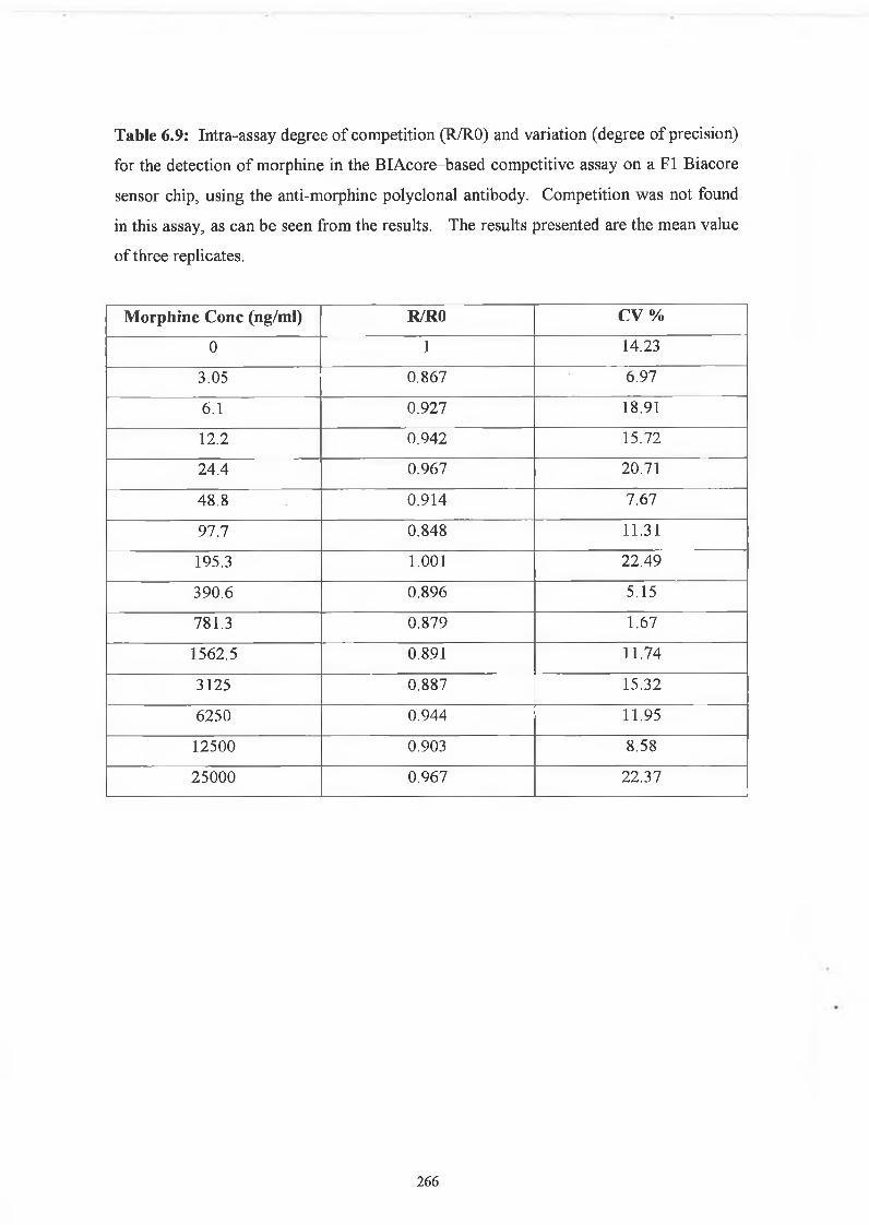
the detection of morphine in saliva samples.

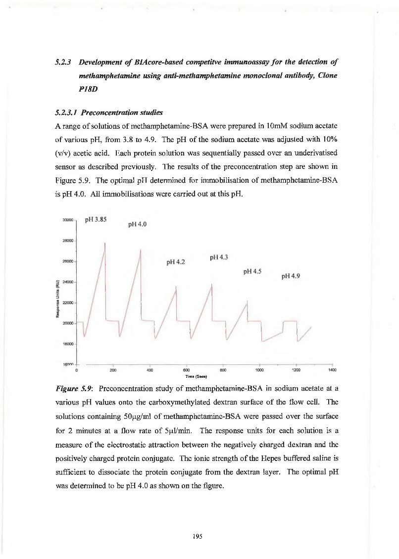
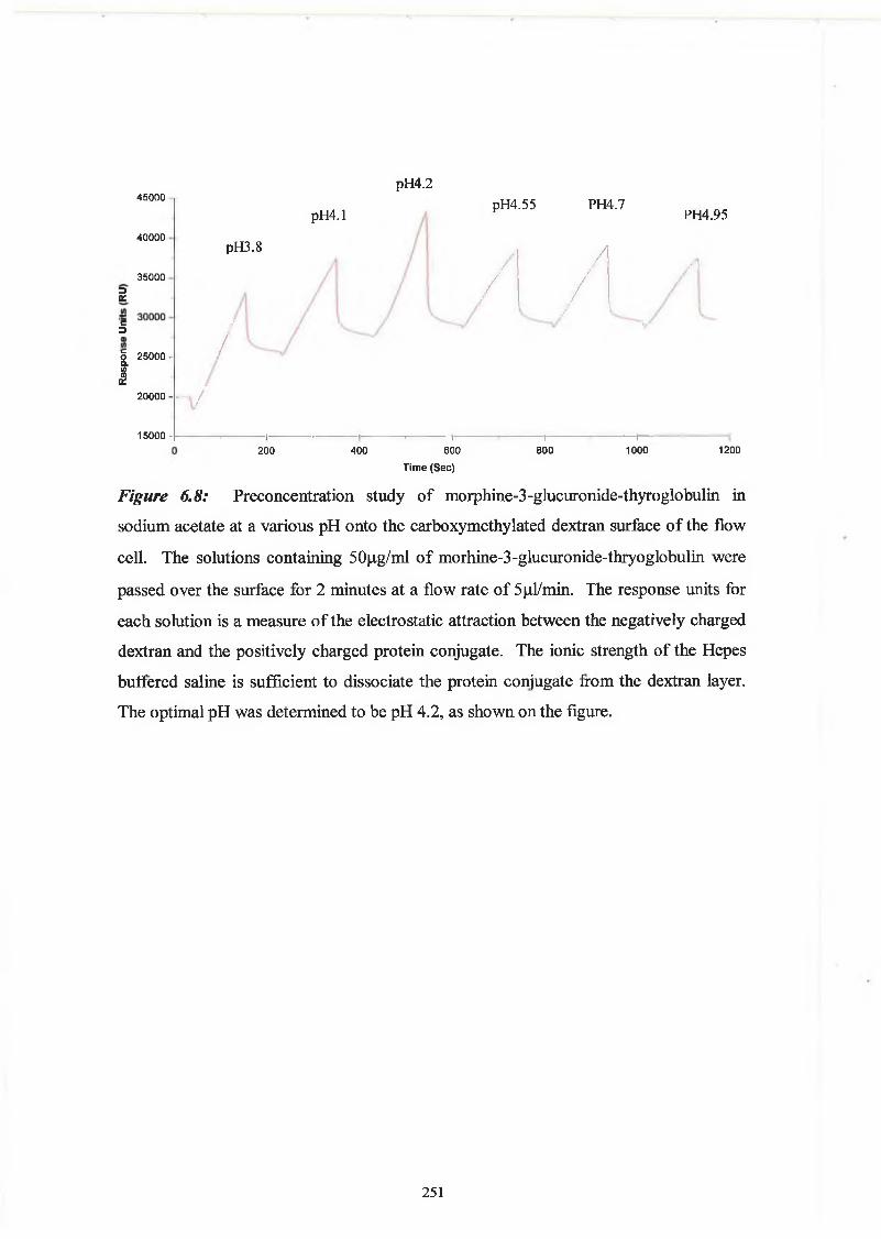
2.10.1 Preconcentration studies

An initial preconcentration step was carried out to determine the optimum pH for the

immobilisation of the drug-protein conjugate. Proteins at pH values below their

isoelectric point, pi, have a positive charge and will be electrostatically attracted to the

negatively charged carboxy groups on the dextran matrix. The pi value of a protein is

often changed by conjugation to a drug so the optimum pH is determined by the

preconcetration study. Drug-protein was dissolved at a concentration of 50 |ig/ml in 10

mM sodium acetate buffer, at a range of pH values between 3.8-5.0. These were passed

sequentially over an underivatised chip surface and the pH giving the highest mass

change in terms of response units (RU) was used for subsequent drug-protein

immobilisation procedures.

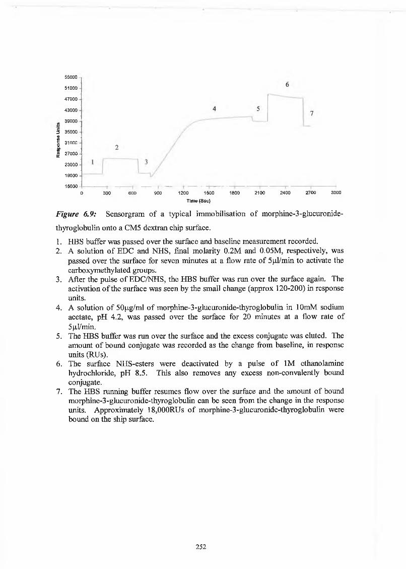
2.10.2. Immobilisation o f drug-protein conjugates

The carboxymethylated dextran was activated, by injecting 35 |ul of a solution

containing 0.05 M NHS and 0.2 M EDC over the chip surfacc at a flow rate of 5 (il/min.

35 (il of a solution of drug-protein in 10 mM acetate buffer, at the appropriate pH, was

passed over the surface at a flow rate of 5 |J,l/min. Unreacted NHS groups were

‘capped’ (Section 4.2.2.), by passing 35 jil of a 1 M ethanolamine (pH 8.5) solution

over the surface at a flow rate of 5 |il/min.

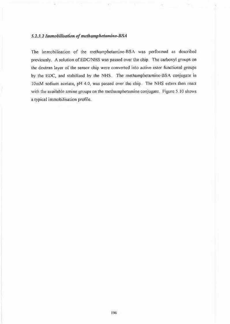
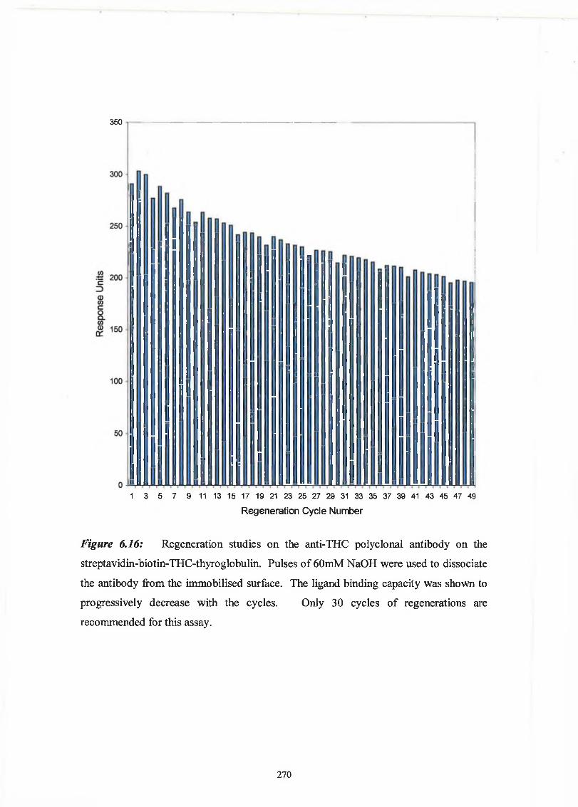
2.10.3. Regeneration Studies

The stability of the immobilised drug-protein conjugates surface, was assessed by

passing a known concentration of antibody over the chip surface and the surface was

62

regenerated with mild acid/base solution as detailed in the results sections. The cycle

of binding and regeneration was performed for approximately 50-100 cycles, and the

binding signal measured to assess the stability of the immobilised surface for assay

development.

2.10.4. Non-Specific binding Studies

Purified monoclonal and polyclonal antibody solutions at the appropriate dilution were

passed over the dextran matrix and the appropriate immobilised protein surface. Non

specific binding to either dextran or immobilised protein surface was eliminated by the

addition of either dextran or protein, or in some cases both, to the antibody solution.

2.10.5. Competitive Assays

Drug solutions was prepared at a series of concentrations ranging from 0.03 - 25,000

ng/ml by serial dilution, using Hepes Buffered Saline (HBS) as diluent. Antibody at a

constant dilution was added to the various antigen concentrations. The antibody:antigen

mixture was allowed to equilibrate for 15 minutes. The equilibrium mixtures were

passed in random order over the chip surface at 5 iitl/min for 4 minutes, and the chip

surface regenerated between cycles by pulses of the appropriate regeneration solution.

The amount of bound antibody was measured in terms of response units (RU). The

response units were divided by the response measured for the antibodyrantigen mixture

containing zero antigen to give normalised binding responses. A plot of antigen

concentration (ng/ml) versus normalised binding responses could then be used to

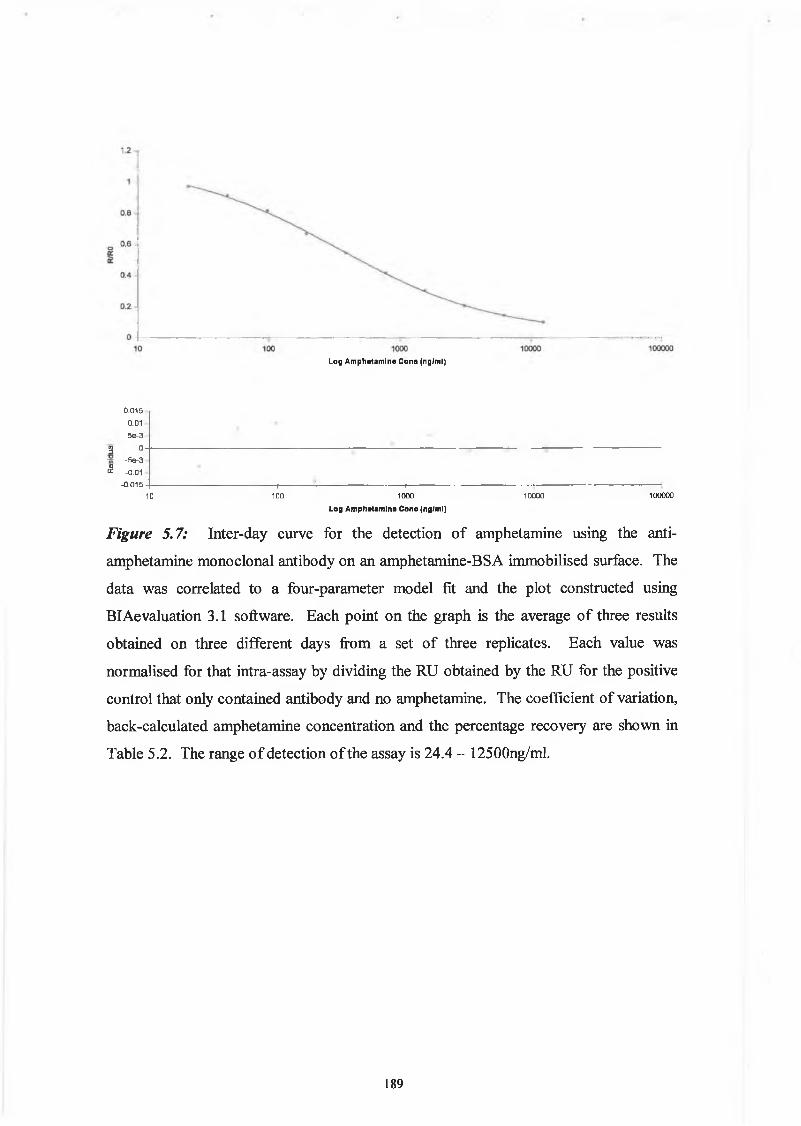
construct the calibration plot using BIAevaluation 3.1 software.

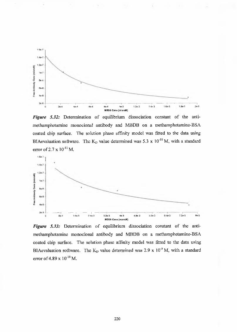
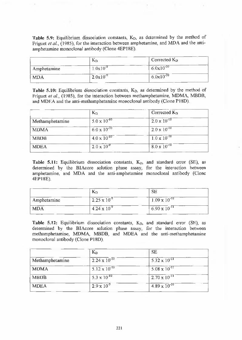
2.10.6. Solution Affinity Analysis using BlAcore

Drug-protein conjugates were immobilised using the conventional EDC/NHS coupling

chemistry. Serial dilutions of the monoclonal antibodies of known concentration

(molarity) were passed over the immobilised surface, and a calibration curve was

constructed of mass bound measured in terms of response units, versus antibody

concentration. A known concentration of antibody was then incubated with varying

63

concentrations of free drug (molarity) and allowed to reach equilibrium overnight. The

equilibrium samples were passed over the immobilised surface and the binding response

calculated. The response values measured were used to calculate the amount of free

antibody in the equilibrium mixtures, from the calibration curve. A graph was then

plotted of drug concentration versus free antibody concentration. The solution phase

interaction models in BIAevaluation 3.1 software, was used to determine the overall

affinity constant, (see Section 5.1.6).

64

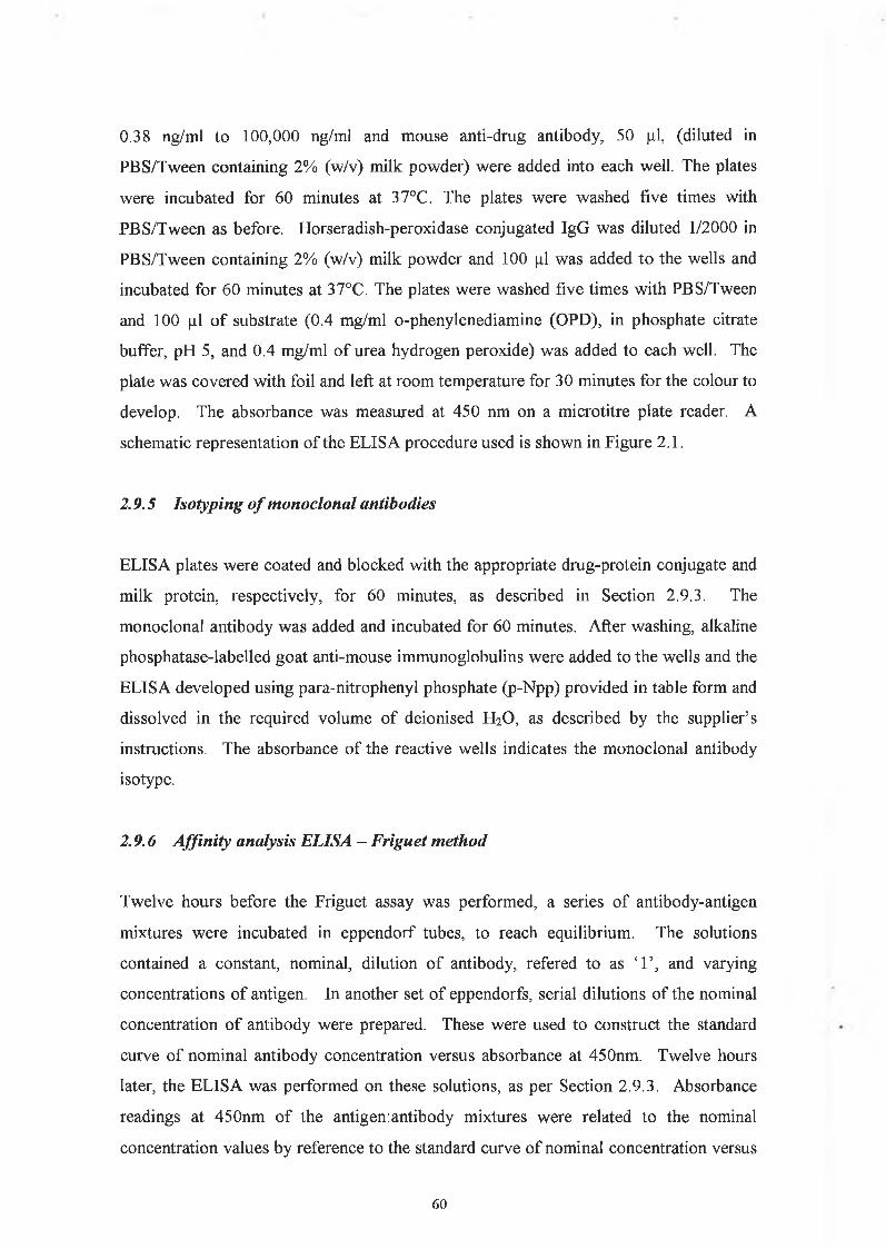
2.11 Collection o f saliva samples

Saliva samples were collected using the saliva collection device from Trinity Biotech.

The absorbant pad was removed and placed in the mouth for a couple of minutes. It

was removed and placed into the plastic ‘filter-like’ component. A second part was

screwed into this container and the saliva collected in an universal tube, through the

pressure of the second part squeezing the saliva from the pad, see Figure 2.1.

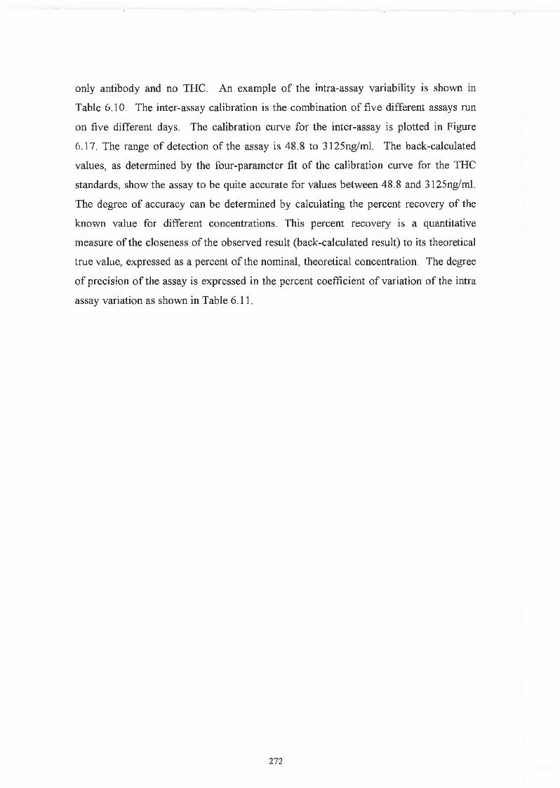
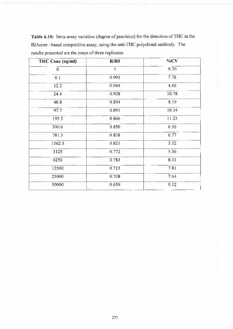
2.12 Development o f Envitec Device Assay fo r detection o f THC

2.12.1 Background to Envitec Device

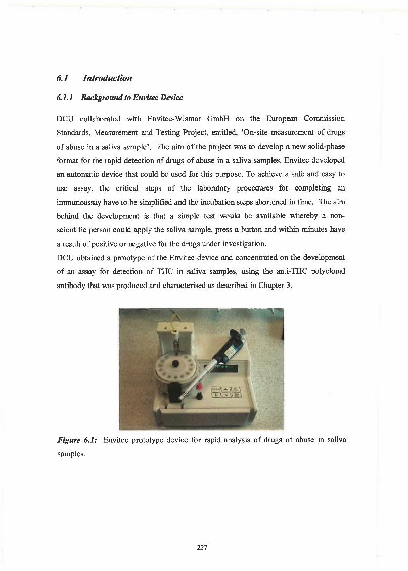
DCU collaborated with Envitec-Wismar GmbH on the European Commission

Standards, Measurement and Testing Project, entitled, ‘On-site measurement of drugs

of abuse in a saliva sample’. The aim of the project was to develop a new solid-phase

format for the rapid detection of drugs of abuse in a saliva samples. Envitec developed

an automatic device that could be used for this purpose. To achieve a safe and easy to

use assay, the critical steps of the laboratory procedures for completing an

immunoassay have to be simplified and the incubation steps shortened in time.

DCU obtained a prototype of the Envitec device and worked on the development of an

assay for detection of THC in saliva samples, using the anti-THC polyclonal antibody

that was produced and characterised as described in

Chapter 3.

65

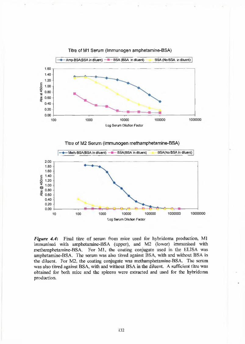
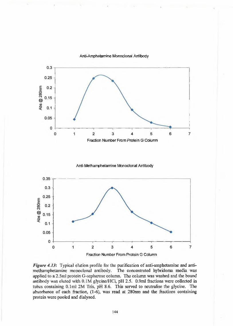
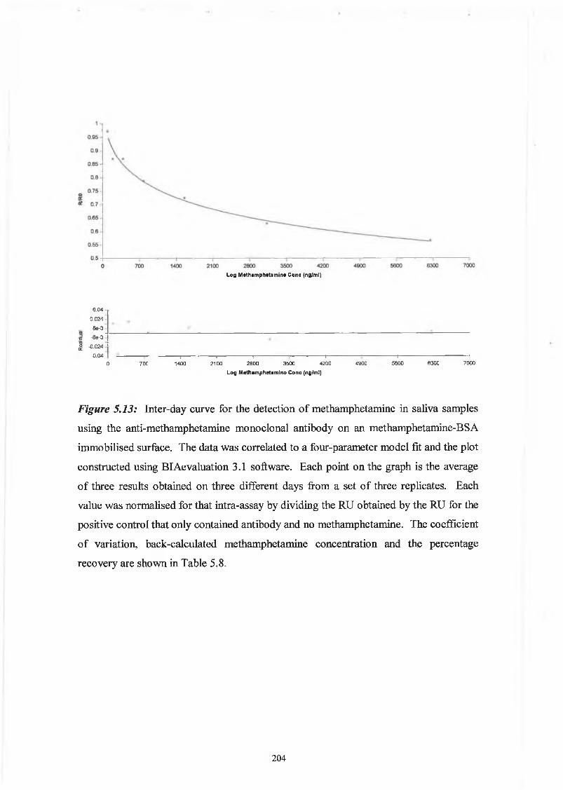
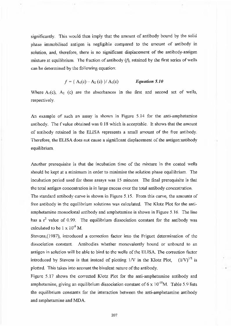
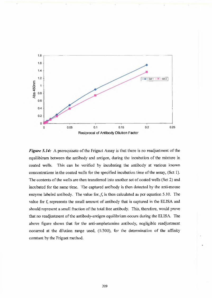
Figurre 2.1: Saliva sample were collected using a saliva collection device (Trinity Biotech, Dublin). The absorbant pad was removed and placed in the mouth for a couple of minutes. It was removed and placed into the plastic filter like component. A second part was screwed into this container and the saliva collected in an universal tube, through the pressure of the second part squeezing the saliva from the pad. The sample collected was diluted 1:1 with PBS and the sample applied to the Envice device for the detection of THC.

66

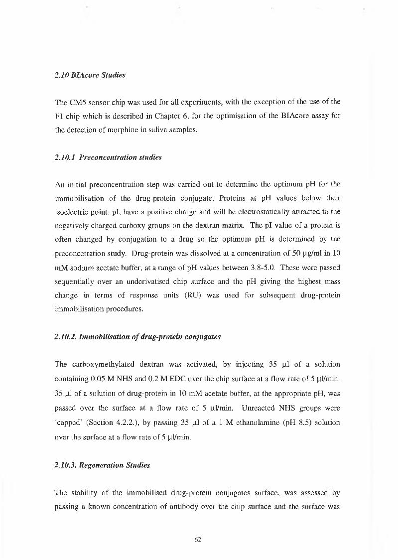
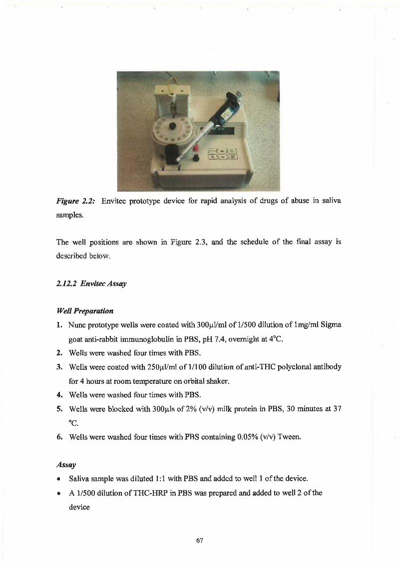
Figure 2.2: Envitec prototype device for rapid analysis of drugs of abuse in saliva

samples.

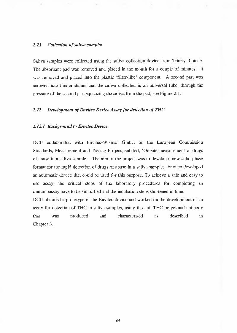
The well positions are shown in Figure 2.3, and the schedule of the final assay is

described below.

2.12.2 Envitec Assay

Well Preparation

1. Nunc prototype wells were coated with 300pl/ml of 1/500 dilution of lmg/ml Sigma

goat anti-rabbit immunoglobulin in PBS, pH 7.4, overnight at 4°C.

2. Wells were washed four times with PBS.

3. Wells were coated with 250|il/ml of 1/100 dilution of anti-THC polyclonal antibody

for 4 hours at room temperature on orbital shaker.

4. Wells were washed four times with PBS.

5. Wells were blocked with 300p,ls of 2% (v/v) milk protein in PBS, 30 minutes at 37

°C.

6 . Wells were washed four times with PBS containing 0.05% (v/v) Tween.

Assay

• Saliva sample was diluted 1:1 with PBS and added to well 1 of the device.

• A 1/500 dilution of THC-HRP in PBS was prepared and added to well 2 of the

device

67

Automated Assay Schedule

• 100|uil of the saliva sample was transferred to wells containing 10()|il THC-HRP.

• The mixture was transferred to the reaction wells.

• The mixture was incubated for 4 minutes.

• The mixture was sent to waste compartment and reaction wells were washed three

limes with Tris Buffer.

• TMB was transferred to reaction wells and the first optical measurement recorded.

• The wells were incubatcd with TMB for five minutes.

• A second optical measurement recorded.

• The results were displayed.

68

wells.Well 1: Saliva sample mixed 1:1 with PBS (minimum 500(j,l needed)Well 2: TMB Substrate (1ml)Well 3: Waste wellWells 4-8: lOOfils THC-HRP (Saliva sample is transferred to these wells for mixing with THC-HRP)Wells 9-13: Reaction wells (coated with anti-THC antibody, after incubation step with sample and THC-HRP mixture, the TMB is transferred here and the transmission read

69

Chapter 3

Production and Characterisation o f Polyclonal Antibodies to

Tetrahydrocannabinol, Cocaine and Morphine

70

3.1 Introduction

3.1.1 The Immune System

The immune system is composed of two levels, the innate and the acquired systems.

The innate system acts as the body’s first line of defence against pathogens. Basic

mechanisms of the innate response include physical barriers such as skin and mucous

membranes and internal mechanisms include phagocytosis, and inflammation.

Phagocytosis involves the internalisation and destruction of foreign matter by cells of

the mononuclear phagoctye system. Natural killer cells are lymphocytes that can

recognise the Class I Major Histocompatability Complex (MHC) molecules on a cell

surface. Cells with reduced MHC molecule expression such as cells that are virally

infected, or cancerous cells, are susceptible to attack by the natural killer cells. In

addition to killing cells, NK cells can also secrete cytokines such as anti-viral cytokine

IFN-y and the inflammatory cytokine TNF-a. The important differentiation between

the innate system and the acquired system is the non-specific nature of the innate

response. The acquired immune system is further divided into humoral immunity and

cell-mediated immunity. The defining characteristics of the acquired immune system

are:

• Specificity

• Inducibility

• Diversity

• Memory

• Distinguish self from non-self

• Downregulation (Elgert, 1996)

The principle components of the humoral immune system are the B lymphocytes and

their products, the antigen-specific antibodies. Cell mediated immunity protects against

intracellular pathogens and release immune system messengers such as cytokines (Th

cells) and kill target cells, (Tc cells).

71

3.1.2 The Lymphoid System

Lymphoid organs are composed of lymphocytes at different stages of development.

They are classified as primary or secondary lymphoid organs. Primary lymphoid

organs are the sites where immune cells, lymphocytes, can mature into functional

effector cells. Generally, T cells are responsible for cell mediated immunity, and B

cells are responsible for the humoral response, although it is critical that there is

interaction between T cells and B cells for antibody production. In humans, the primary

lymphoid organs are the bone marrow and thymus. B cells are produced and mature in

the bone marrow. The precursors of T cells, produced also in the bone marrow transfer

to and mature in the thymus. The secondary lymphoid organs include the spleen, lymph

nodes, and mucosal-associated lymphoid tissue, (MALT), and it is at these sites that the

lymphocytes can interact with antigens and undergo differentiation. The lymph nodes

primarily respond to antigens in the tissue that they serve. The spleen acts as a filter for

the circulatory system. The MALT system organises antibodies at major entry points of

antigen entry (Roitt, 1994; Kimball, 2002).

3.1.3 Antibody production and the Humoral immune system

The specificity, diversity and memory are the key characteristics of the acquired

immune response. As described below haptens less than 5Kda in size are usually

unable to illicit an immune response. Adjuvants are oil/water emulsions with microbial

components, e.g., heat killed Mycobacterium tuberculosis, in Freund’s complete

Adjuvant. They are used to increase the immunogenicity of the substance, by localising

the injection in the emulsion, and the microbial components cause an increase in the

initial response involving the macrophages. The primary response of the body to a

foreign agent primes the immune system for subsequent immunisations.

B cell receptors bind antigens and engulf them by endocytosis. The antigen is digested

into fragments and they are displayed at the cell surface in conjunction with a class II

MHC molecule. Helper T cells (Th cells) specific for this structure bind the B cell and

secrete lymphokines that stimulate the B cell to develop into a clone of cells with

identical antibodies and differentiate into plasma cells that secrete these antibodies.

72

There are two kinds of TH cells: TH1 cells that participate in cell mediated immunity and

Th 2 cells that are essential for antibody-mediated immunity.

When the precursors to TH cells are presented with an antigen, by an antigen presenting

cell, they proliferate and become activated. Depending on the origin of the APC, the TH

cell will develop into TH 1 or Th 2 cells.

Th 1 cells are produced when the APC presents antigen to the Tcell receptor for antigen

in combination with the activation by EL-12. The Th 1 cells then secrete tumor-necrosis

factor-beta (TNF-(3 ) and interferon-gamma (IFN-y )

These stimulate phagocytosis by macrophages and recruit other lymphocytes to the site

producing inflammation.

Th 2 cells are produced when another type of APC present antigen to the T cell's

receptor for antigen.

The major lymphokines secreted by Th 2 cells are IL-4, IL-5, IL-10 and IL-13.

Interleukin 4 (IL-4): Stimulates class-switching in B cells and promotes synthesis of

IgE antibodies. It also acts as a positive-feedback device promoting more TH cells to

enter the Th 2 pathway. It also inhibits expression of the IL-12 receptor thus inhibiting

cells from entering the Thl path.

Interleukin 5 (IL-5): Attracts and activates eosinophils

Interleukin 10 (IL-10): Inhibits IL-12 production by APCs. This inhibits cells from

entering the Th 1 pathway.

Interleukin 13 (IL-13): Promotes the synthesis of IgE antibodies.

The foreign material is engulfed by macrophages and displayed on antigen presenting

cells in conjunction with the Class II MHC receptor. These are presented and bind to

Th cells and initiate a series of immune responses leading to T cell proliferation and

release of interleukin-1 (IL-1). This results in subsequent release of IL-2. The

activated Tc cells respond directly in the cell-medicated immune response by acting as

cytotoxic cells. The antigen also binds specifically to the B lymphocytes, and after the

activation and presentation of the antigen to Th cells, the B lymphocytes convert to

plasma cells through the critical interaction of Th cells and IL-4 and IL-5. The plasma

73

cells secrete the specific antibodies. Some of the cells remain as memory B cells that

are ready in case of future exposure to the specific antigen (Kimball, 2002).

3.1.4 A ntibody Diversity

The range of antigens that are presented to lymphocytes is huge and so the immune

system must be capable of responding through its ability to reorganise the DNA

material responsible for the production of immunoglobulins. The human genome has

the DNA information to encode for all the immunoglobulins, however they are not

organised into genes, but rather the genes are assembled from different sections of

DNA.

For the antibody chains the gene segments are composed of variable (V) segments.

Each of these encodes most of the N-terminal of the antibody, including the first two

(but not the third) hypervariable region. The diversity (D) gene segments encode part of

the third hypervariable region. The joining (J) gene segments encodes the remainder of

the V region including the remainder of the hypervariable region. The constant (C)

regions encode the remaining constant region of the antibody.

Four mechanisms contribute to this antibody diversity. The obvious processes to

contribute to this diversity, are the many different V, D, and J germline gene sequences,

and secondly the combinatorial recombination of these gene segments and chain

association (Figure 3.1). The different combinations of V and J segments combining

for constant light chains and V, D, and J segments joining for heavy chains, and then

subsequent random association of the different light and heavy chains leads to a large

diverse range of immunoglobulins. Another process contributing to the diversity is

junctional diversity. This happens when there is imprecise DNA rearrangement

involved in the joining of V with J, D with J, or V with D. Another contributor to

junctional diversity is the insertion of random nucleotide regions between V, or J and D

DNA segments in heavy chain genes. Finally the other contributory factor of overall

antibody diversity is somatic mutation. The mutants created as the B cells divide allow

for the selection by antigen of antibodies that provide better binding (Elgert, 1996).

74

V ]0

V H. ^H2 V h3 II u C(IgG) - C(IgA) - C(IgM)

I DNA Rearrangement

V||. I I -------IcqgO)

IVm miC(IgG)

Imessenger RNA

H2n | y | c l COOH Heavy chain of IgG

Figure 3.1: Recombinational arrangement of the DNA encoding variable, (V), diversity,

(D), junction, (J) and constant (C ) regions of an immunoglobulin heavy chain and the

subsequent transcription to messenger RNA and translation into the heavy chain.

3.1.5 Antibody Structure

The structural characterisation of antibodies began in the 1930s with work performed by

Tiselius & Kabat. They did electrophoretic studies on non-immunised and post

immunisation rabbit serum, and found that there was an increase in the gamma-globulin

fraction following immunisation. This led to one characterisation of them as gamma

globulin. The chemical structure was further investigated by Porter, Edelman, and

Nisonoff in the 1950s and 60s, (Elgert, 1996). Porter digested the immunoglobulin with

the proteolytic enzyme, papain, to cleave the peptide bonds, producing three fragments,

two antigen binding Fab fragments and a non-antigen-binding Fc fragment. Edelman

disrupted the disulphide bonds with dithiothrietol, iodoacetamide, and a denaturing

agent, producing the two heavy chains and two light chains. Nisonoff used pepsin to

hydrolyse the antibody at different sites to the papain and this hydrolysis resulted in one

75

large fragment called F(ab/, that could bind antibody, and other smaller fragments. It

could be further reduced to yield two Fab-like fragments called Fab .

The basic structure of an antibody is shown in Figure 3.2. The heavy and light chains

are made up of repeated domains, each about 110 amino acids in length. The heavy

chains have one variable region and three constant domains. The light chain has one

variable domain and one constant domain. The variability of the antigen binding site is

located in the complementarity-determining regions (CDRs), sub-divided into CDR1,

CDR2, and CDR3. The variable regions of the chains are responsible for the antigen

recognition and the constant regions are central to the biological effector functions.

Binding to antigen is also facilitated by the flexible movement of the two Fab portions,

which can change angle of between 60 to 180 degrees.

Immunoglobulins are divided into five groups based on their isotype. Isotypic

determinants distinguish C-region sites on a heavy chain. The five groups are IgG, IgA,

IgM, IgD and IgE. Subdivisions of these classes exist also. Antigenic determinants on

light chains distinguish them as either k or X. Different isotypes have different

functions. IgG is the major immunoglobulin in the blood and is primarily induced by

antigens. IgA is dimeric and is usually found in body fluids such as saliva and tears,

and acts to guard these areas of the body. IgM is a pentamer and is the activator of

complement. IgD is found on the surface on B cells where it is thought to be involved

in regulation of B cell activity. IgE is found in hypersensitivity allergic reactions (Roitt,

1994; Kimball, 2002).

Table 3.1: Classification and characteristics of immunoglobulins.

Class Hchain L chain Characteristic

IgG gamma kappa or lambda

Most common antibody seen, transferred across placenta

IgM mu kappa or lambda

Pentamer antibody, appears in primary response after immunization

IgA alpha kappa or lambda

Dimer antibody, found in secretions such as saliva,tears

IgD delta kappa or lambda Uncertain function

IgE epsilon kappa or lambda

Involved in allergic reactions by binding to mast cells and sensitizing them

76

CDRRegions

Figure 3.2: Structure of the immunoglobulin molecule. The antibody is composed of

two light chains and two heavy chains. The variable regions are located at the amino

acid terminal end of the molecule. The light chain is composed of one variable region

and one constant region. The heavy chains are composed of one variable region and

three constant regions. The hinge region allows flexibility in the molecule for antigen

binding. The antigen binding sites are specific and are represented by the

complementarity-determining regions (CDR) regions. The heavy and light chains are

connected via disulphide bonds, and there are disulphide bridges at the hinge region

also between the two heavy chains. Disulphide bonds are also present in the constant

and variable regions.

77

3.1.6 Drug protein conjugation

Haptens are small chemical compounds, less than 5 KDa in size. They must be

conjugated to a large carrier protein to be rendered immunogenic. To elicit an immune

response the drugs examined in this study need to be conjugated to protein. The use of

a drug-protein conjugate as an immunogen results in antisera containing a mixture of

antibodies specific for the drug, protein and linking region between the drug and

protein.

In the design of the conjugate, several factors need to be considered. The reactive

groups and the positions on the drug provide a starting point for the design. The drugs

under study were coupled through a carboxyl group to the amine groups on the proteins.

This proceeded through EDC/NHS coupling chemistry. For the application of

polyclonal antibodies in an ELISA format it is necessary to use conjugates differing

from the immunogens with regard to the protein used and if possible the linkage

between the drug and hapten. Bovine thyroglobulin, bovine serum albumin and keyhole

limpet haemocyanin are proteins that could be used for the production of hapten-protein

conjugates. For the purposes of screening a more soluble protein such as bovine serum

albumin is suitable for the ELISA format, as it is water soluble. Dextran has a low

immunogenicty, (P. Dillion, Personal Communication) and when conjugated to a hapten

can be used as a screening conjugate for the identification of hybridomas specific for

the drug of interest. The likelihood of the antibodies produced recognising the dextran

part of the conjugate is small therefore eliminating the occurrence of positives that do

not recognise the free drug. This is true of many ‘polymer-type’ substances, in that they

do not make good immunogens (Hermanson, 1996). Ethylenediamine can be used as a

linker between the drug and protein.

The procedures for the conjugation of a drug to a protein are well documented,

(Hermanson, 1996). The usual method involves linking the drug to a carrier protein via

a peptide bond. To perform this conjugation the drug must have suitable carboxyl or

primary amino groups. If they are not present, the drug must first be derivatised to

synthetically produce a derivative that contains those groups. The choice of

derivatisation site on the hapten is of utmost importance in the design of an immunogen.

Care must be taken not to derivatise those groups that distinguish a molecule from its

relatives. The hapten should be linked to the carrier protein according to Landsteiner's

78

principle which states that ‘antibody specificity is directed primarily at the portion of

the hapten furthest removed from the functional group that is used to link the hapten to

the carrier protein’ (Erlanger, 1980). Exposed sites act as antigenic determinants and are

available to circulating lymphocytes, so antibodies to these are produced in numbers.

The ideal epitope density per molecule is in the range 8-25 haptens per protein. This

ratio seems to affect only the time taken for a suitable immune response to be generated.

As little as two haptens per protein can generate a response but it will be delayed,

(Erlanger, 1980).

By preparing a conjugate that has a structure common to the parent drug and it’s

metabolites, antibodies with a general specificity for a drug and its metabolites will be

produced. Fasciglone et al. (1996), reported that the immunogenicity of a conjugate is

related to the hydrophobicity of the carrier. They concluded that hydrophobic haptens

hide inside carrier proteins by interactions with the hydrophobic segments, resulting in

no immunogenic response. It would, therefore, follow that for the generation of an

immunogenic response against a hydrophobic hapten, it would be advisable to use a

hydrophilic carrier protein.

Ethylenediamine can be as a means of introducing a linker into the drug-protein

conjugate. The ethylenediamine initially cationises the ovalbumin The carboxylate

groups of the protein are modified by the ethylendiamine by the formation of amide

bonds with an alkyl spacer containing a terminal primary amine group. This blocking

of the carboxyl groups on the protein and the addition of terminal primary amines raises

the pi value. The highly positive charge of the cationised protein has been shown to

significantly increase its immunogenicity. (Hermanson, 1996) When haptens are

coupled through the cationised protein amine residues, the charge still remains high and

produces a greater immune response. The positive charge assists in its binding to the

antigen presenting cells and gets processed at an increased rate.

The production of antibodies to the main metabolite of heroin, morphine, provides a

challenge regarding antibody production, due to its closeness in structure to the legal

medication codeine. Findlay et al. (1981) investigated the relationships between

immunogen structures and the resulting antibodies in the area of opioids. They found

that conjugates of codeine-6-hemisuccinate, ethylmorphine-6-hemisuccinate or

oxycodone-6-carboxymethyloxime had greater recognition of structural changes around

the piperidine ring nitrogen atom and the 14-position. N-carboxypropylnormorphine-

BSA, N-carboxypropylnorcodeine-BSA and norcodeine-BSA elicited antibodies that

79

recognised changes in the 14-substituent. Codeine conjugated through the 8 position

elicited antibodies similar to those elicited by N-carboxypropylnorcodeine-BSA.

Salamone et al. (1998) reported the use of a non-cannabinoid immunogen used to

generate antibodies with broad cross reactivity to the cannabinoid metabolites. They

derivatised a benzpyran structure to elicit antibodies that were directed towards the

conserved epitopes of cannabinoid metabolites. These antibodies showed two to three

times higher cross reactivity with the cannabinoids than traditional phenolie-linked or 9-

position-linked immunogens.

The design of a immunogen can be assessed by molecular modeling studies, however,

the success of the immunogen can only be measured by the resulting titre of the

antiserum produced.

Figure 3.3: The carbodiimide method for conjugating haptens and proteins through

their carboxyl and amine groups, respectively. The process is mediated by EDC and

NHS.

8 0

In the following results section, the production of morphine-protein and cocaine-protein

conjugations are outlined. The immunisations and resulting titres of rabbit serum are

presented. The purification process of the antibodies and the subsequent

characterisation of the anti-THC, anti-morphine and anti-cocaine polyclonal antibodies

are described. These antibodies were applied to an ELISA format and an assay

developed and optimised for the detection of THC, morphine and cocaine.

81

3.2 Results

3.2.1 Drug protein conjugate production

The following schemes outline the process for the conjugation of cocaine and morphine

to proteins, through EDC/NHS chemistry. Commercial conjugates of THC were

obtained for the purposes of this project as there was difficulties encountered sourcing

sufficient quantities of these drugs.

3.2.1.1 EDC/sulfo-NHS coupling chemistry

EDC (l-ethyl-3-(3-dimethylaminopropyl) carbodiimide hydrochloride)/NHS((N-

hydroxysulfosuccinimde) coupling chemistry is used to conjugate the drug and protein.

The scheme used is outlined in Figure 3.3 (Hermanson, 1996). EDC reacts with the

carboxylic group to form an active o-acylisourea ester intermediate. To stabilize the

intermediate, sulfo-NHS is added and a stable sulfo-NHS ester intermediate is formed.

The sulfo-NHS esters are hydrophilic active groups that react rapidly with the amines

on the protein.

3.2.1.2 Conjugation o f morphine to protein

Morphine contains the following groups

• Tertiary amino group

• Phenolic group (crucial to analgesic activity)

• Alcohol group

• Aromatic ring (Receptor sites in the brain)

• Ether bridge

• Double bond

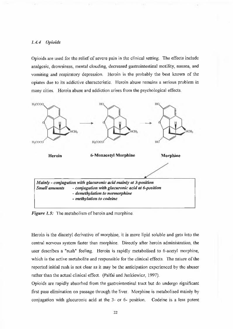
Heroin is a powerful analgesic with twice the effects of morphine. Heroin differs from

morphine in two areas. The 3-OH (Phenolic OH group) has become acetylated and the 6

alcohol has also been acetylated. Morphine has three polar groups (phenol, alcohol and

an amine) whereas analogues have either lost the polar alcohol group or have masked it

by an alkyl or acyl group. Heroin has two polar groups. The brain barrier is fatty, and

82

the significance of the polar groups becomes clear, the more polar morphine molecule is

prevented from entering the brain, whereas the less polar heroin can enter easily.

For the purposes of generating a morphine-protein conjugate, morphine-3-glucuronide

was used as the starting material. The glucuronide group provides an ideal reactive

group for conjugation through EDC/NHS chemistry, as described later. It also provides

an excellent linker region for the purposes of screening for antibodies specific for

morphine and not the area between the morphine and BSA. The utilisation of the

conjugate in the ELISA format was validated by performing an ELISA using the

morphine-3-glucuronide-OVA as the coating conjugate and the commercial morphine

antibody as the primary antibody.

An ELISA was performed to assess the success of the above conjugation. The

morphine-3-glucuronide-thyroglobulin was used as the coating conjugate and

commercial anti-morphine monoclonal antibody was used as the primary antibody. The

ELISA was performed as described in Section 2.9. The results can be seen in Figure

83

M-3-G-Thy 50ug/ml — M-3-G-Thy 10ug/ml M-3-G-Thy 5ug/ml M-3-G-Thy 1 ug/ml X Thy 10Oug/ml

Log Commercial anti-Morphine Monoclonal Antibody Dilution Factor

Figure 3.4: ELISA to confirm the conjugation of morphine to thyroglobulin. ELISA

plates were coated with different concentrations of ‘lab-produced’ morphine-

thyroglobulin conjugate. Commercial anti-morphine monoclonal antibody was used

in the ELISA. The response to the thyroglobulin part of the conjugate was also

measured by coating another series of wells with throglobulin alone. The response to

the ‘lab-produced’ conjugate was positive, indicating a successful conjugation.

84

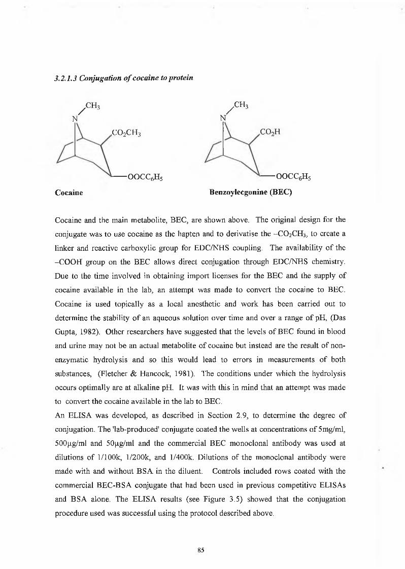
3.2.1.3 Conjugation o f cocaine to protein

/-CH3

/,c h 3

N N

,co 2c h 3

o o c c 6h 5

,c o 2h

o o c c 6h 5

Cocaine Benzoylecgonine (BEC)

Cocaine and the main metabolite, BEC, are shown above. The original design for the

conjugate was to use cocaine as the hapten and to derivatise the -CO2CH3, to create a

linker and reactive carboxylic group for EDC/NHS coupling. The availability of the

-COOH group on the BEC allows direct conjugation through EDC/NHS chemistry.

Due to the time involved in obtaining import licenses for the BEC and the supply of

cocaine available in the lab, an attempt was made to convert the cocaine to BEC.

Cocaine is used topically as a local anesthetic and work has been carried out to

determine the stability of an aqueous solution over time and over a range of pH, (Das

Gupta, 1982). Other researchers have suggested that the levels of BEC found in blood

and urine may not be an actual metabolite of cocaine but instead are the result of non-

enzymatic hydrolysis and so this would lead to errors in measurements of both

substances, (Fletcher & Hancock, 1981). The conditions under which the hydrolysis

occurs optimally are at alkaline pH. It was with this in mind that an attempt was made

to convert the cocaine available in the lab to BEC.

An ELISA was developed, as described in Section 2.9, to determine the degree of

conjugation. The 'lab-produced' conjugate coated the wells at concentrations of 5mg/ml,

500(.ig/ml and 50jj.g/ml and the commercial BEC monoclonal antibody was used at

dilutions of l/100k, l/200k, and l/400k. Dilutions of the monoclonal antibody were

made with and without BSA in the diluent. Controls included rows coated with the

commercial BEC-BSA conjugate that had been used in previous competitive ELIS As

and BSA alone. The ELISA results (see Figure 3.5) showed that the conjugation

procedure used was successful using the protocol described above.

85

B E C -B S A 5m g/m l — ■ — B E C -B S A 500u g /m l B E C -B S A 50ug /m l

C om m B E C -B S A 10ug /m l — W— C om m B E C -B S A 5ug/m l — • — B S A 1ÛOug/ml

Dilution Factor of Commercial anti-BEC MAb

Figure 3.5: ELISA to confirm the conjugation of cocaine to bovine serum albumin

(BSA). ELISA plates were coated with different concentrations of ‘lab-produced’

BEC-BSA conjugate and commercial BEC-BSA conjugate. Commercial anti-BEC

monoclonal antibody was used in the ELISA. The response to the BSA part of the

conjugate was also measured by coating another series of wells with BSA alone. The

response to the ‘lab-produced’ conjugate was positive, indicating a successful

conjugation.

86

3.2.2 Determination o f rabbit antibody titres

Rabbits were immunised with the following drug-protein conjugates for the production

of polyclonal antibodies. For the production of anti-THC antibodies, the immunogen

used was THC-BTG, (Fitzgerald Industries). For the production of anti-BEC

antibodies, the initial immunogen used was BEC-BSA, (Fitzgerald Industries) and later

immunisations were prepared with the BEC-BSA that was produced as described in

Section 2.5.2. The immunogen used to induce anti-morphine antibodies was initially

morphine-BSA, (Fitzgerald Industries), and following the initial boosts, morphine-3-

glucuronide-BSA was used.

Figure 3.6 show the antibody titre from a rabbit immunised with THC-BTG. The serum

was diluted in PBS/Tween containing 0.1% (w/v) BSA to remove non-specific

interactions with the protein part of the conjugate. It was also titred against BSA, with

and without BSA in the diluent. This was to detect any immune response to the protein

part of the conjugate, and to ensure that 0 .1 % (w/v) was sufficient to remove the non

specific interactions. Although there was a response to the protein, it could be

eliminated by the addition of the protein to the diluent. As can seen from Figure 3 .6, a

very good response was obtained, the rabbit immunised with THC-BTG had a final titre

of approximately 1/6 million.

Figures 3.7 and Figure 3.8 show the antibody titre from a rabbit immunised with BEC-

BSA. The serum was diluted in PBS/Tween containing 0.1% (w/v) BSA to remove non

specific interactions with the protein part of the conjugate. It was also tested against

BSA, with and without BSA in the diluent. This was designed to detect any immune

response to the protein part of the conjugate, and to ensure that 0.1% (w/v) of BSA was

sufficient to remove non-specific interactions. The response was greater to the protein

carrier than it was to the drug, as can be seen from the figures. Figure 3.7 shows the

final titre that was obtained and screened using BEC-BgG as the screening conjugate.

The rabbit immunised with BEC-BSA had a disappointing final titre of approximately

1/50,000. It was decided to discontinue the immunisation schedule at that point as all

titres had shown a much greater response to the BSA protein carrier than to the BEC

drug hapten.

Figures 3.9 show the antibody titre from a rabbit immunised with morphine-BSA. It

was screened against the morphine-3-glucuronide-ovalbumin conjugate. The rabbit

immunised with morphine-BSA had a final titre of 1/400,000.

87

A final titre from the rabbit serum should be preferably in the region of 1/500,000.

Experience by our research group and others have shown that a prolonged immunisation

schedule of about six months is preferable (Danilova, 1994). This leads to greater

affinity of the antibodies.

♦ THC-BSA, BSA in diluent - ■ BSA, BSA in diluent BSA, No BSA in diluent

Log Serum Dilution Factor

Figure 3.6: Titre of serum from rabbit immunised with THC-BTG

(tetrahydrocannabinol-bovine thyroglobulin). BSA was incorporated into the diluent

buffer to eliminate the binding interaction between the antibody and the protein

carrier. The serum was also titered against BSA, with and without BSA in the diluent.

This showed that the response to the protein could be eliminated by incorporating the

protein into the diluent.

88


Figure 3.7: Titre of serum from rabbit immunised with BEC-BSA (benzoylecgonine- bovine serum albumin). BSA was incorporated into the diluent buffer to eliminate the binding interaction between the antibody and the protein carrier. The serum was also titered against BSA, with and without BSA in the diluent. This showed that the response to the BSA could be eliminated by incorporating the BSA into the diluent.


Figure 3.8: Titre of serum from rabbit (2A) immunised with BEC-BSA(benzoylecgonine-bovine serum albumin) and screened against BEC-BgG.

89

Abs

@ 45

0nm

Log Sérum Dilution Factor

Figure 3.9: Titre of serum from rabbit immunised with morphine-BSA and screened

against morphine-3-glucuronide-ovalbumin.

90

3.2.3 Purification and characterisation o f polyclonal antibodies

The anti-THC, anti-BEC and anti-morphine polyclonal antibodies were purified by

applying the dialysate from the ammonium sulphate precipitation to a Protein G

immobilised Sepharose 3B column. The polyclonal antibodies were eluted from the

column with 0.1M glycine, pH 2, as described in Section 2.8.3. The fractions collected

were neutralised with 2M Tris, pH 8 .6 . The fractions were then read

spectrophotometrically at 280 nm to determine the protein content. The fractions

containing protein were pooled and dialysed in PBS overnight at 4°C with two of

changes of PBS.

The purified antibodies were run on an SDS-PAGE to determine purity, as shown in

Figure 3.10 and 3.11.

Lane 1: anti-amphetamine MAb Lane 2:anti-amphetamine MAb Lane 3:anti-BEC PAb Lane 4: anti-BEC Pab Lane 5 Markersa 2-Macroglobulin human plasma, 180KDa P-Galactosidase (E. coli), 116KDa Fructose-6-phosphatase (Chicken), 84KDa Pyruvate kinase (Chicken), 54KDa Fumerase (Porcine), 48.5KDa Lactic Dehydrogenase (Rabbit), 36.5KDa Triosephosphate isomerase (Rabbit), 26.6KDa

Figure 3.10: Characterisation by SDS-PAGE gel of the anti-BEC polyclonal

antibody. Two bands can be seen, the top one at 50KDa representing the heavy chain

and the lower band at 25KDa representing the light chains.

91

LANE 1 6 7

66,000

45.000

.14.700

24.000

9

1 & 7:Molecuiar weight markers

Heavy Chain

L ig h t C h a in

Morphine antiserum Supernatant from first SAS cut wash Supernatant from second SAS cut wash Purified anti-morphine polyclonal antibody Purified anti-THC polyclonal antibody

Figure 3.11: Characterisation by SDS-PAGE gel of the anti-morphine and anti-THC

polyclonal antibody. Two bands can be seen, the top one at 50KDa representing the

heavy chain and the lower band at 25KDa representing the light chains.

92

3.2.4 Development o f ELISAs fo r the detection o f THC, morphine and cocaine

using the polyclonal antibodies

3.2.4.1 Anti-THCpolyclonal antibody

For the development of an ELISA for the detection of THC, the optimal coating

concentration of THC-BSA and the optimal antibody dilution was determined by an

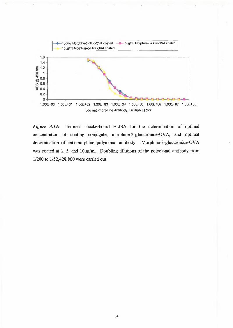
indirect checkerboard ELISA. The results can be seen in Figure 3.12, the conjugate

coating concentration ranged from 1 p-g/ml to 10 (ig/ml. The coating concentrations

gave similar sensitivities and due to the expenses and availability of the conjugate,

1 pg /ml was chosen as the concentrations for ELISAs. The optimal antibody dilution

was approximately 1/5000, as this gave an absorbance in the 0.5 range and this is

considered to be the sensitive region of the curve. However, for the purposes of

optimisation of the assay with regard to sensitivities and cut off levels, the competitive

assay was performed using a 1/10000 dilution of the polyclonal antibody and a less

dilute secondary antibody dilution of 1/2000. Figure 3.6, the titre of the serum from this

rabbit showed that at this concentration the response to the BSA carrier protein was

negligible.

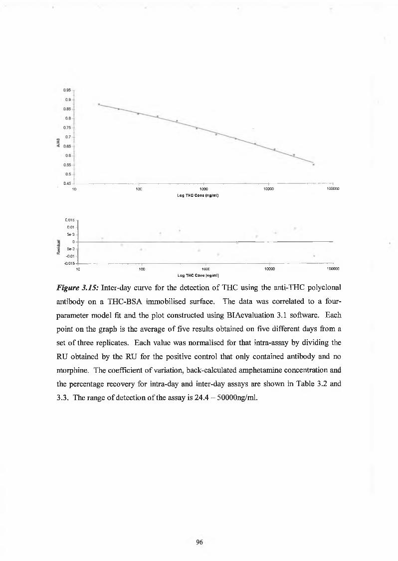
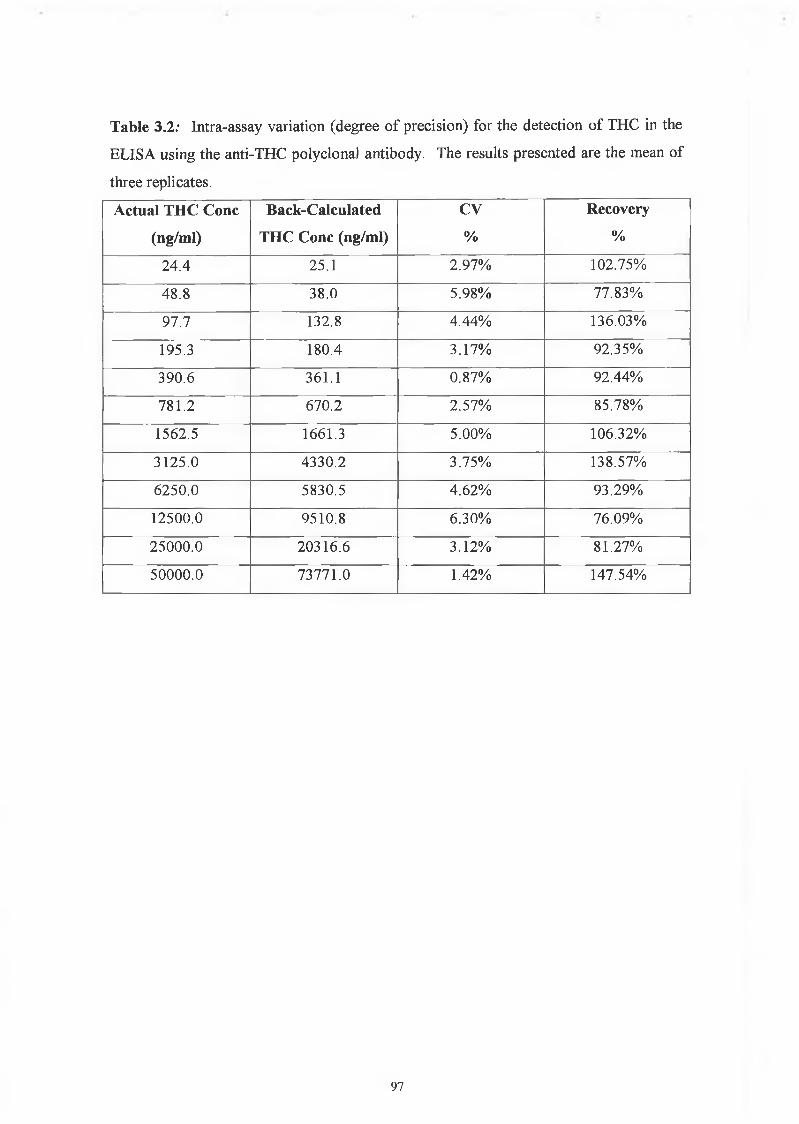
Figure 3.15 shows the relationship between the absorbance at 450nm and the

concentration of free THC as determined by the competitive ELISA format. The range

of detection of the assay was found to be between 24 and 50000 ng/ml. The intra-assay

variation was determined from three replicates in an assay while the inter-assay

variation was determined over five days of performing the assay. The intra-assay and

inter-assay coefficients of variation are listed in Table 3.2 and 3.3.

93

— • — 10ug/ml THC-BSA coated — 5ug/ml THC-BSA coated 1ug/ml THC-BSA coated

Log anti-THC Antibody Dilution Factor

Figure 3.12: Indirect checkerboard ELISA for the determination of optimal

concentration of coating conjugate, THC-BSA, and optimal determination of anti-THC

polyclonal antibody. THC-BSA was coated at 1, 5, and 10pg/ml. Doubling dilutions of

the polyclonal antibody from 1/200 to 1/52,428,800 were carried out.

1 ug/ml BEC-BgG coated —■— 5ug/ml BEC-BgG coated 10ug/ml BEC-BgG coated

Log anti-BEC Antibody Dilution Factor


concentration of coating conjugate, BEC-BgG, and optimal determination of anti-BEC

polyclonal antibody. BEC-BgG was coated at 1, 5, and lOfxg/ml. Doubling dilutions of

the polyclonal antibody from 1/200 to 1/52,428,800 were carried out.

94

1 ug/ml Morphine-3-Gluc-OVA coated — 5ug/m! Morphine-3-Gluc-OVA coated10ug/ml Morphine-3-Gluc-OVA coated

1.00E+00 1.00E+01 1.00E+02 1.00E+03 1.00E+04 1.00E+05 1.00E+06 1.00E+07 1.00E+08Log anti-morphine Antibody Dilution Factor


concentration of coating conjugate, morphine-3-glucuronide-OVA, and optimal

determination of anti-morphine polyclonal antibody. Morphine-3-glucuronide-0VA

was coated at 1, 5, and 10fig/ml. Doubling dilutions of the polyclonal antibody from

1/200 to 1/52,428,800 were carried out.

95

0 .4 5 n------------- — ----------- I----------------- ■— t— r 1 v ■ ------------- *---------- *------ ---------------- — '— ■ ■ -»-'*-8— -------------------- ------------------------------------------------— --------------------------------------------• — ■*i- ’— i -~ ------------------- ------------------------------------------------1— >— ’— '-110 100 1000 10000 100000

L o g T H C C o n o (n g /m l)

0 .01 5

0.01

5e-3

ro 0 ------------------------------------------------------------------------------------------------------------------------------------------------------------------- ------------------------------------TJ1 -5e-3a:

- 0.01

-0 .0 1 5 — -------------------------------- ■ * i - r----------------------- ----------- - - - - ------- " — ' - - ■ --------- 110 100 1000 10000 100000

L o g T H C C o n e (n g /m l)

Figure 3.15: Inter-day curve for the detection of THC using the anti-THC polyclonal

antibody on a THC-BSA immobilised surface. The data was correlated to a four-

parameter model fit and the plot constructed using BIAevaluation 3.1 software. Each

point on the graph is the average of five results obtained on five different days from a

set of three replicates. Each value was normalised for that intra-assay by dividing the

RU obtained by the RU for the positive control that only contained antibody and no

morphine. The coefficient of variation, back-calculated amphetamine concentration and

the percentage recovery for intra-day and inter-day assays are shown in Table 3.2 and

3.3. The range of detection of the assay is 24.4 - 50000ng/ml.

Table 3.2: Intra-assay variation (degree of precision) for the detection of THC in the

ELISA using the anti-THC polyclonal antibody. The results presented are the mean of

three replicates.

Actual THC Cone

(ng/ml)

Back-Calculated

THC Cone (ng/ml)

CV

%

Recovery

%

24.4 25.1 2.97% 102.75%

48.8 38.0 5.98% 77.83%

97.7 132.8 4.44% 136.03%

195.3 180.4 3.17% 92.35%

390.6 361.1 0.87% 92.44%

781.2 670.2 2.57% 85.78%

1562.5 1661.3 5.00% 106.32%

3125.0 4330.2 3.75% 138.57%

6250.0 5830.5 4.62% 93.29%

12500.0 9510.8 6.30% 76.09%

25000.0 20316.6 3.12% 81.27%

50000.0 73771.0 1.42% 147.54%

97

Table 3.3: Inter-assay variation (degree of accuracy and reproducibility) for the

detection of THC in the ELISA using the anti-THC polyclonal antibody. The results

presented are the mean values obtained from five intra-day assays, each assay had three

replicates. The range of detection of the assay is 24.4 - 50000.0 ng/ml.

Actual THC Cone

(ng/ml)

Back-Calculated

THC Cone (ng/ml)

CV

%

Recovery

%

24.4 22.3 9.34% 91.46%

48.8 51.9 8.06% 106.27%

97.7 114.0 6.53% 116.71%

195.3 164.8 7.55% 84.37%

390.6 318.9 8.96% 81.64%

781.25 902.6 5.54% 115.54%

1562.5 1897.6 4.10% 121.45%

3125.0 3193.9 5.25% 1 0 2 .2 1 %

6250.0 5764.3 4.11% 92.23%

12500.0 11013.2 2.71% 88 .1 1 %

25000.0 20677.2 3.63% 82.71%

50000.0 61160.4 2.46% 122.32%

98

3.2.4.2 Anti-cocaine polyclonal antibody

The optimal coating concentration of BEC-BgG and the optimal antibody dilution was

determined by an indirect checkerboard ELISA. The results can be seen in Figure 3.12,

the conjugate coating concentration ranged from 1 |ig /ml to 10 pig /ml. The coating

concentrations gave similar sensitivities and due to the expenses and availability of the

conjugate, 5 (j,g /ml was chosen as the concentrations for ELISAs. The optimal

antibody dilution was 1/1000, as this gave an absorbance in the 0.5 range. However, in

order to develop the competitive assay to detect free cocaine it was necessary to use a

dilution of antibody at 1/500. The relationship between the absorbance at 450 nm and

the concentration of cocaine is shown in Figure 3.16. This shows that a satisfactory

competitive ELISA can be used with an antibody dilution of 1/500. The range of

detection of the assay was between 6.1 to 25000 ng/ml. The intra-assay variation was

determined from three replicates in an assay while the inter-assay variation was

determined over five days of performing the assay. The intra-assay and inter-assay

coefficients of variation are listed in Table 3.4 and 3.5.

Another series of experiments were devised to look at an assay format using the

immunogen, BEC-BSA, as the coating conjugate with and without BSA in the diluent.

Figure 3.7 shows that the response to the BSA-coated plate was greater that that to the

BEC-BSA-coated plate, although this could be relieved by incorporating 1% (w/v) BSA

into the diluent. Prior titres performed on the serum from animals immunised with this

BEC-BSA conjugate also showed greater binding to the BSA. This means that there

was a greater immune response towards the BSA part rather than the hapten. When a

competitive assay format was investigated using the BEC-BSA as the coating

conjugate, it was found that competition did not occur between the conjugate and the

free cocaine.

99

0.1 :10 1000

L og C o c a in e C o n e (ng /m l)

10000 100000

100 1000 10000 100000

Log C o c a in e C o n e (ng /m l)

Figure 3.16: Inter-day curve for the detection of morphine using the anti-BEC

polyclonal antibody on an BEC-BgG (benzoylecgonine-bovine gamma globulin)

immobilised surface. The data was correlated to a four-parameter model fit and the

plot constructed using BIAevaluation 3.1 software. Each point on the graph is the

average of five results obtained on five different days from a set of three replicates.

Each value was normalised for that intra-assay by dividing the RU obtained by the

RU for the positive control that only contained antibody and no morphine. The

coefficient of variation, back-calculated amphetamine concentration and the

percentage recovery are shown in Table 3.4 and 3.5. The range of detection of the

assay is 6.1 - 25000ng/ml.

0.015 0.01 5e-3 ■

0-5 e -3- 0,01

-0 .01 510

100

Table 3.4: Intra-assay variation (degree of precision) for the detection of cocaine in the

ELISA using the anti-BEC polyclonal antibody. The results presented are the mean

values of three replicates.

Actual Cocaine

Cone (ng/ml)

Back-Calculated

Cocaine Cone

(ng/ml)

CV

%

Recovery

%

6 .10 7.97 5.02% 130.69%

12 .2 0 9.70 1.35% 79.50%

24.41 22.85 1.44% 93.62%

48.83 52.47 2.82% 107.45%

97.65 91.64 5.82% 93.85%

195.31 219.05 1.99% 112.16%

390.62 417.69 0.84% 106.93%

781.25 543.01 0.45% 69.51%

1562.50 1755.70 2.44% 112.36%

3125.00 5632.17 0 .00% 180.23%

6250.00 7442.83 1.72% 119.09%

12500.00 7928.00 4.36% 63.42%

25000.00 18029.05 4.42% 72.12%

101


detection of cocaine in the ELISA using the anti-BEC polyclonal antibody. The results

presented are the mean values obtained from five intra-day assays, each assay had three

replicates.

Actual Cocaine

Cone (ng/ml)

Back-Calculated

Cocaine Cone

(ng/ml)

% CV % Recovery

6 .10 7.31 6.39% 119.85%

12 .2 0 11.69 6.29% 95.84%

24.41 21.36 9.71% 87.48%

48.83 53.34 12.84% 109.24%

97.65 92.95 13.01% 95.18%

195.31 202.95 10.48% 103.91%

390.62 393.24 1 0 .0 1 % 100.67%

781.25 709.07 5.88% 90.76%

1562.50 1704.25 7.30% 109.07%

3125.00 3647.00 10.60% 116.70%

6250.00 5803.12 13.28% 92.85%

12500.00 9060.86 16.26% 72.49%

25000.00 33737.83 13.94% 134.95%

102

3.2.4.3 Anti-morphine polyclonal antibody

The optimal coating concentration of morphine-3-gluc-OVA and the optimal antibody

dilution was determined by an indirect checkerboard ELISA. The results can be seen in

Figure 3.13, the conjugate coating concentration ranged from 1 [ig/ml to 10 (ig/ml. The

coating concentrations gave similar sensitivities and 1 (ig/ml was chosen as the

concentrations for ELISAs. The optimal antibody dilution was approximately 1/3200.

However, for the purposes of optimisation of the assay with regard to sensitivities and

cut off levels, the competitive assay was performed using a 1/1500 dilution of the

polyclonal antibody.

Figure 3.17 shows the relationship between the absorbance at 450nm and the

concentration of free morphine as determined by the competitive ELISA format using

the antibody dilutions listed above. The range of detection of the assay was found to be

between 0.38 and 6250 ng/ml morphine. The intra-assay variation was determined from

three replicates in an assay while the inter-assay variation was determined over five

days of performing the assay. The intra-assay and inter-assay coefficients of variation

are listed in Table 3.6 and 3.7, and show the assay to be reproducible and accurate, as

determined by the acceptable percentage recoveries and coefficient of variations.

103

010 100 1000

Log M orphine C o n e (ng/m l)

0.02

0.012

4©-3

1 ---------------------------------------------------------------------------- ’&o>K -0.012

- 0 . 0 2 --------------------------------------- • ------------------ -------------- • • • • r --------------- - ---- -----------------------------------

10 100 1000 10000Log M o rp h in e C o n e (ng/rnl)

Figure 3.17: Inter-day curve for the detection of morphine using the anti-morphine

polyclonal antibody on an morphine-3-glucuronide-OVA immobilised surface. The

data was correlated to a four-parameter model fit and the plot constructed using

BIAevaluation 3.1 software. Each point on the graph is the average of three results

obtained on three different days from a set of three replicates. Each value was

normalised for that intra-assay by dividing the RU obtained by the RU for the positive

control that only contained antibody and no morphine. The coefficient of variation,

back-calculated amphetamine concentration and the percentage recovery are shown in

Table 3.6 and 3.7. The range of detection of the assay is 0.38 - 6250ng/ml.

104

Table 3.6: Intra-assay variation (degree of precision) for the detection of morphine in

the ELISA using the anti-morphine polyclonal antibody. The results are obtained from

three replicates.

Actual Morphine

Cone (ng/ml)

Back-Calculated

Morphine Cone

(ng/ml)

CV

%

Recovery

%

0.38 0.23 1.63% 60.00%

0.76 1.0 2 3.96% 133.82%

1.52 2.42 2.30% 159.47%

3.05 2.66 1.51% 87.28%

6 .10 5.90 0 .00% 96.64%

12 .2 0 11.62 1.39% 95.26%

24.41 22.55 0.83% 92.39%

48.83 57.16 3.66% 117.06%

97.65 96.22 0 .00% 98.54%

195.31 176.62 0.55% 90.43%

390.62 364.64 1.81% 93.35%

781.25 894.13 1.40% 114.45%

1562.50 2056.40 0.97% 131.61%

3125.00 3390.73 2.05% 108.50%

6250.00 3744.29 2.76% 59.91%

105


detection of morphine in the ELISA using the anti-morphine polyclonal antibody. The

range of detection of the assay is 0.38 - 6250.0 ng/ml. The results presented are the

mean values obtained from five intra-day assays, each assay had three replicates.

Actual Morphine

Cone (ng/ml)

Back-Calculated

Morphine Cone

(ng/ml)

CV

%

Recovery

%

0.38 0.35 6.19% 91.05%

0.76 1 .0 2 5.82% 134.74%

1.52 1.99 5.32% 131.05%

3.05 3.60 4.74% 118.00%

6 .10 6.87 5.17% 112.54%

12 .2 0 12.24 5.44% 100.30%

24.41 21.93 5.31% 89.85%

48.83 51.99 10.77% 106.46%

97.65 90.61 7.81% 92.79%

195.31 184.08 9.04% 94.25%

390.62 406.15 8.91% 103.98%

781.25 961.24 8.85% 123.04%

1562.50 1820.32 8.56% 116.50%

3125.00 3033.26 9.62% 97.06%

6250.00 3740.58 9.82% 59.85%

106

3.2.4.4 Cross reactivity studies: Anti-morphine polyclonal antibody

The cross reactivity of the anti-morphine polyclonal antibody was determined against

morphine-3-glucuronide, 6-MAM, norcodeine and codeine. The degree of cross

reactivity was determined as per the competitive ELISA described in Section 2.9.4. The

standards were obtained from a stock solution of lmg/ml standard in ethanol. The

degree of cross reactivity was determined as the concentration of cross reactant that

gives a response of 50% or one-half of the observed maximum binding, (EC50 - Cross

Reactant) expressed a percentage of the specific analyte concentration that gives a 50%

response, (EC50 - Specific Analyte).

% Cross Reactivity = Concentration of Analyte ( E C 50 - SA) X 100%

Concentration of Cross Reactant ( E C 50 - CR)

The degree of cross reactivity of the anti-morphine antibody is expressed in Table 3 .8.

Table 3.8: Cross reactivity of anti-morphine polyclonal antibody.

Drug % Cross Reactivity Range of Detection

(ng/ml)

Morphine-3-glucuronide 10 0% 97.7-6250.0

6-monoacetylmorphine

(6-MAM)

30.39% 48.8 -1562.5

Norcodeine 0.78% 195.3-12500

Codeine 10 0% 390.1

107

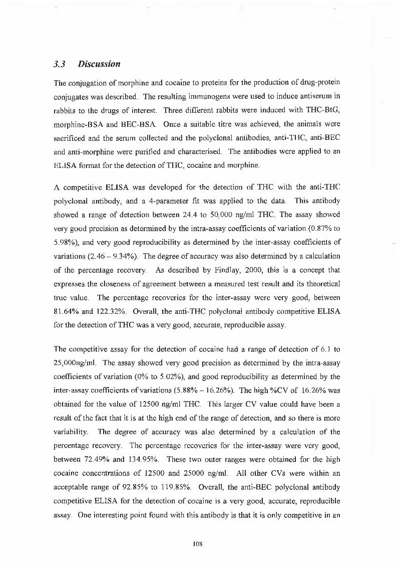
The conjugation of morphine and cocaine to proteins for the production of drug-protein

conjugates was described. The resulting immunogens were used to induce antiserum in

rabbits to the drugs of interest. Three different rabbits were induced with THC-BtG,

morphine-BSA and BEC-BSA. Once a suitable titre was achieved, the animals were

sacrificed and the serum collected and the polyclonal antibodies, anti-THC, anti-BEC

and anti-morphine were purified and characterised. The antibodies were applied to an

ELISA format for the detection of THC, cocaine and morphine.

A competitive ELISA was developed for the detection of THC with the anti-THC

polyclonal antibody, and a 4-parameter fit was applied to the data. This antibody

showed a range of detection between 24.4 to 50,000 ng/ml THC. The assay showed

very good precision as determined by the intra-assay coefficients of variation (0.87% to

5.98%), and very good reproducibility as determined by the inter-assay coefficients of

variations (2.46 - 9.34%). The degree of accuracy was also determined by a calculation

of the percentage recovery. As described by Findlay, 2000, this is a concept that

expresses the closeness of agreement between a measured test result and its theoretical

true value. The percentage recoveries for the inter-assay were very good, between

81.64% and 122.32%. Overall, the anti-THC polyclonal antibody competitive ELISA

for the detection of THC was a very good, accurate, reproducible assay.

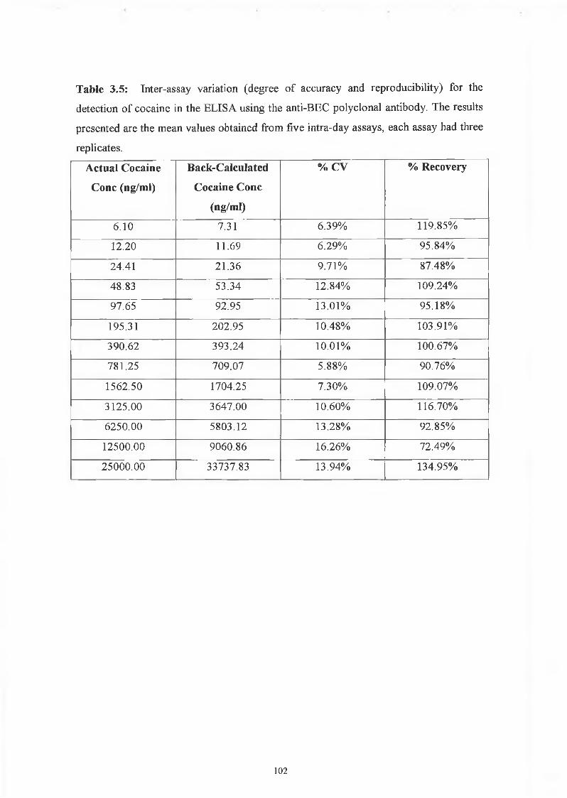
The competitive assay for the detection of cocaine had a range of detection of 6.1 to

25,000ng/ml. The assay showed very good precision as determined by the intra-assay

coefficients of variation (0% to 5.02%), and good reproducibility as determined by the

inter-assay coefficients of variations (5.88% - 16.26%). The high %CV of 16.26% was

obtained for the value of 12500 ng/ml THC. This larger CV value could have been a

result of the fact that it is at the high end of the range of detection, and so there is more

variability. The degree of accuracy was also determined by a calculation of the

percentage recovery. The percentage recoveries for the inter-assay were very good,

between 72.49% and 134.95%. These two outer ranges were obtained for the high

cocaine concentrations of 12500 and 25000 ng/ml. All other CVs were within an

acceptable range of 92.85% to 119.85%. Overall, the anti-BEC polyclonal antibody

competitive ELISA for the detection of cocaine is a very good, accurate, reproducible

assay. One interesting point found with this antibody is that it is only competitive in an

3.3 Discussion

108

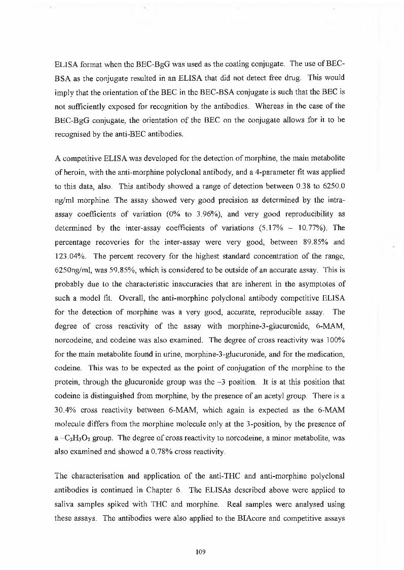
ELISA format when the BEC-BgG was used as the coating conjugate. The use of BEC -

BSA as the conjugate resulted in an ELISA that did not detect free drug. This would

imply that the orientation of the BEC in the BEC-BSA conjugate is such that the BEC is

not sufficiently exposed for recognition by the antibodies. Whereas in the case of the

BEC-BgG conjugate, the orientation of the BEC on the conjugate allows for it to be

recognised by the anti-BEC antibodies.

A competitive ELISA was developed for the detection of morphine, the main metabolite

of heroin, with the anti-morphine polyclonal antibody, and a 4-parameter fit was applied

to this data, also. This antibody showed a range of detection between 0.38 to 6250.0

ng/ml morphine. The assay showed very good precision as determined by the intra

assay coefficients of variation (0% to 3.96%), and very good reproducibility as

determined by the inter-assay coefficients of variations (5.17% - 10.77%). The

percentage recoveries for the inter-assay were very good, between 89.85% and

123.04%. The percent recovery for the highest standard concentration of the range,

6250ng/ml, was 59.85%, which is considered to be outside of an accurate assay. This is

probably due to the characteristic inaccuracies that are inherent in the asymptotes of

such a model fit. Overall, the anti-morphine polyclonal antibody competitive ELISA

for the detection of morphine was a very good, accurate, reproducible assay. The

degree of cross reactivity of the assay with morphine-3-glucuronide, 6-MAM,

norcodeine, and codeine was also examined. The degree of cross reactivity was 100%

for the main metabolite found in urine, morphine-3-glucuronide, and for the medication,

codeine. This was to be expected as the point of conjugation of the morphine to the

protein, through the glucuronide group was the -3 position. It is at this position that

codeine is distinguished from morphine, by the presence of an acetyl group. There is a

30.4% cross reactivity between 6-MAM, which again is expected as the 6-MAM

molecule differs from the morphine molecule only at the 3-position, by the presence of

a -C 2H3O2 group. The degree of cross reactivity to norcodeine, a minor metabolite, was

also examined and showed a 0.78% cross reactivity.

The characterisation and application of the anti-THC and anti-morphine polyclonal

antibodies is continued in Chapter 6 . The ELISAs described above were applied to

saliva samples spiked with THC and morphine. Real samples were analysed using

these assays. The antibodies were also applied to the BIAcore and competitive assays

109

were established for the detection of the drugs. Chapter 6 also describes the application

of the anti-THC antibody to the Envitec Device for the development of a novel rapid

assay.

110

Chapter 4

Production and Characterisation o f Anti-Amphetamine

and Anti-Methamphetamine Monoclonal Antibodies

u i

4.1 Introduction

4.1.1 Monoclonal Antibodies - Background

The 1984 Nobel Prize in Physiology and Medicine was awarded to Georges Kohler and

Cesar Milstein for their pioneering work to produce an immortalised monoclonal

antibody producing cell (Kohler & Milstein, 1975). Their work revolutionised antibody

production and the associated areas where the antibodies can be applied. Monoclonal

antibodies are antibodies of a single idiotype produced by immortalised B cells.

Normal B cells are the end products of a differentiation pathway and cannot be

maintained in culture. Myeloma cells are immortal, but the antibodies produced are of

unknown specificity. Kohler and Milstein harnessed the pertinent qualities of each of

the cells, and fused the B cells producing antibody of desired specificity with the

myeloma cells. The result is a hybrid-mye\-oma, called a hybridoma.

Interestingly, at the time of publication of the original work, the National Research

Development Council, the organisation through which the Medical Research Council

scientists could commercially exploit their work, wrote ‘It is certainly difficult for us to

identify any immediate practical application which could be pursued as a commercial

venture’ (Austin, 1989).

4.1.2 Production o f monoclonal antibodies

The production of monoclonal antibodies begins with immunisation of mice by either

in-vivo or in-vitro immunisations. In-vivo immunisations are carried out at regular time

intervals, usually at least 4-6 weeks apart for several months. The success of the

immunisations can be monitored by taking samples of serum and following the titre of

the antibodies produced. There are publications detailing shorter immunisation periods

by more frequent immunisations, (Wring et al., 1999). Normally, for the isolation of

spleenocytes, a longer time-scale is more beneficial, with regard to the affinity of the

antibodies produced. It is also possible to produce an hybridoma from other lymphoid

tissue such as lymph nodes.

The fusion between the spleenocytes and the myeloma cells e.g., Sp2/0-Agl4, is usually

achieved through the use of polyethylene glycol, which causes a change in membrane

112

permeability. The original method for fusion was inactivated Sendai virus, which

induces intercellular fusion in activated cells. However, the receptors for the Sendai

virus fusion protein are needed and since some cells lack these proteins the fusion agent

used now is PEG. Electroporation is another method that is used to promote fusion,

though to a lesser extent (McCullough and Spier, 1990).

The fusion process is a relatively random process and the fused hybridoma cells must be

selected from the unfused B cells and myeloma cells. The selection process used by

Kohler and Milstein is accomplished by culturing the hybridoma cells in hypoxanthine-

aminopterin-thymidine medium (HAT). Aminopterin blocks the de novo biosynthesis

of the purines and pyrimidines that are required for DNA synthesis. When this pathway

is blocked the cells can use the salvage pathway using the exogenous hypoxanthine and

thymidine, however they need the enzymes hypoxanthine-guanine phosphoribosyl

transferase (HGPRT) and thymidine kinase (TK) to do this (Figure 4.1). The myeloma

cells chosen for a fusion deliberately lack the hypoxanthine-guanine phosphoribosyl

transferase enzyme (HGPRT'). So, in the HAT medium the uniused myeloma cells die,

as do any myeloma cells fused to other myeloma cells. The spleenocytes possess the

HGPRT enzyme, however they have a limited time in culture and will eventually die

after about 2 weeks. The myeloma cells that fused with spleenocytes now possess the

HGPRT enzyme and can grow in the HAT medium.

The hydridoma cells are grown in HAT medium for about two weeks. This ensures that

all hybridomas that revert to a myeloma phenotype are eliminated. The media is then

changed to HT media for at least another seven feedings and sub-cultures at which time

any traces of aminopterin should have been eliminated (McCullough and Spier, 1990).

The process for producing a monoclonal antibody is outlined in Figure 4.2 and

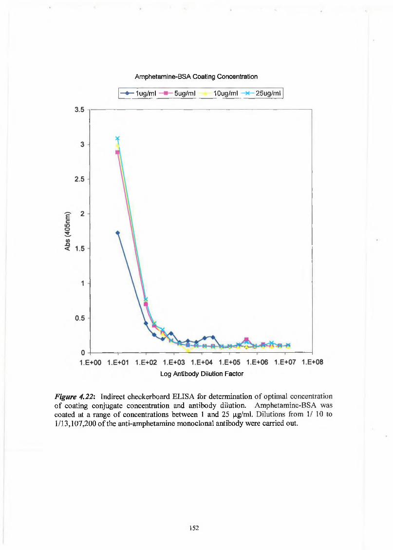
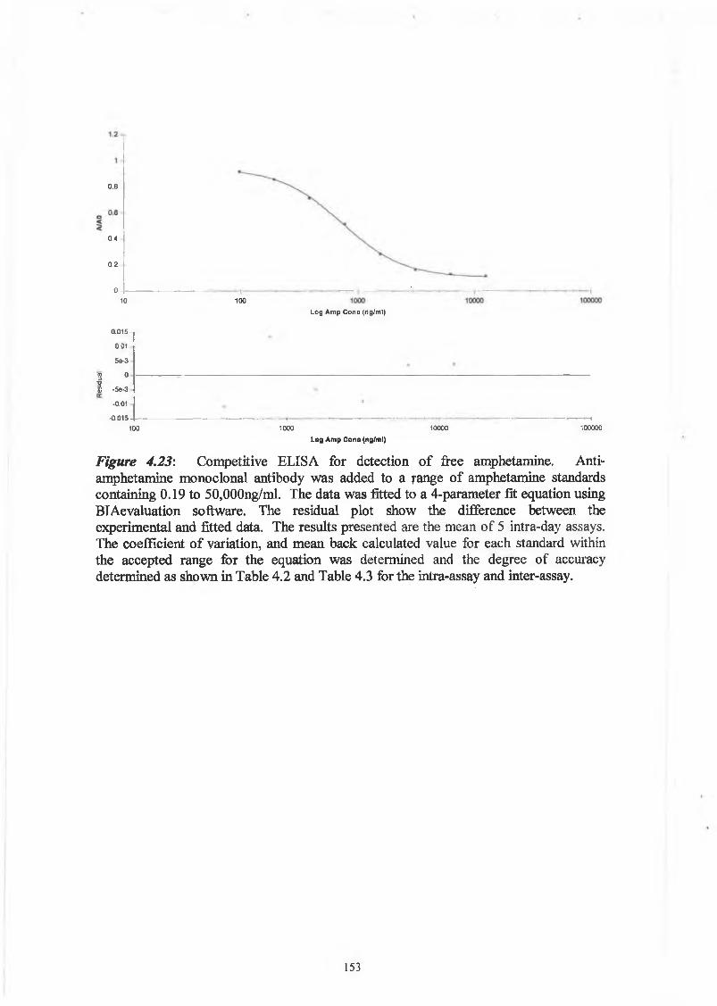
described in detail in Chapter 2.

113

HypoxanthineHGPRT

Ribonucleotides

IDe novo synthesis Anflfifttefflin DNA

tRibonucleotides

Thymidine Kinase Thymidine

Figure 4.1: In the presence of aminopterin, the de novo biosynthesis of purine and

pyrimidines is blocked. Hypoxantihne and thymidine are needed for the salvage

pathway, as are the enzymes HGPRT and thymidine kinase. Cells lacking these

enzymes will die in HAT medium because they are incapable of producing the nucleic

acids. It is through this process that fused myeloma cells are selected. The myeloma

cells are HGPRT' and so only those fused with the HGPRT+-B cells survive in the

HAT medium.

114

SpleenExtracted

1

Approx Ixl06-lxl08 spleenocytes per typical spleen

1

ego □

Fusion performed by addition of PEG at specific time intervals

1

o 0 0 o 0 0 0 0 0 0 o 00 o 0 0 o 0 0 o o o 0 0o 0 o o 0 o 0 0 o 0 o 0o o o 0 0 o 0 o 0 0 0 00 0 o o 0 0 0 0 0 0 o 00 o 0 0 0 o 0 o o o 0 0o 0 o 0 0 o 0 0 0 0 0 0

! 00 o o o o o 0 o 0 0 0

Fusion Ratio of 10 Spleenocytes to 1 SP2 Cell

Fused hybridoma cells, incubated for 7 days in HAT medium

1Screening performed for specific hybridomas and first cloning step performed ¡sr

After at least three rounds of cloning specific monoclonal antibody is produced and characterised

Figure 4.2: Principle of monoclonal antibody production.

115

An alternative to in vivo immunisation is in vitro immunisation of cultured spleenocytes

(Borrebaeck, 1988). This procedure has several advantages over in vivo immunisations:

• It follows a reduced immunisation schedule leading to less time needed prior to

fusion.

• It uses smaller amounts of the antigen of interest. This is particularly important as

many substances are in extremely short supply due to expense or purification

methods.

• It allows the production of antibodies to weakly immunogenic agents, to self-

antigens and to toxic agents that cannot be immunised in vivo.

• It avoids the ethical arguments associated with in vivo immunisation (Borrebaeck,

1988).

The main disadvantage however, is that the primary immunological response is

obtained, which means that IgM antibodies are produced rather than IgG antibodies that

are usually produced by the in vivo immunisation method. This means that the

antibodies produced have a greater chance of being polyreactive, (Bouvet and Dighiero,

2000). McMahon and O’Kennedy (2001) looked at a panel of nine hybridomas,

secreting IgM anti-goat IgG, that had been produced from splenocytes that had been

immunised in vitro with the goat IgG. The affinity constants of the antibodies against

six antigens were examined and the specific anti-IgG activities of the hybridoma

supernatant and corresponding affinity purified IgM fraction were determined. Nine

antibodies were tested, eight were found to be polyreactive. The degree of

polyreactivity may be underestimated by screening techniques such as ELISA as

discussed in the next section.

4.1.3 Screening fo r antibodies o f interest

The successful fusion of the myeloma cells and spleenocytes produces a range of

hybridomas that secrete antibodies. The splenocytes are a heterogenous group of cells

and so a different antibody is produced by each hybridoma. The mice used for the

fusion would have been immunised for up to several months and kept in the laboratory

animal facility and so would have been exposed to somewhat different environmental

and endogenous factors along with the immunogen. This exposure means the immune

116

system is responding to other immunogens. There is also the issue that not all

hybridomas will produce any antibody at all. The hybridoma cell when formed is

tetraploid, because it is formed from two diploid cells. As the cells grow and divide, the

extra chromosomes are lost. This means that some cells die, some stop producing the

antibody and other successful ones go on to produce the antibody of interest. All of

these factors mean that the screening procedure for the selection of hybridomas is of the

utmost importance. The screening step is also the most time-consuming stage of

hybridoma production and has to be performed alongside the continued cultures of the

hybridomas. When the specific hybridoma cells are identified the cloning procedures

must begin in order to isolate the single hybridoma that is secreting the required

antibody. Screening must continue during this step as the hybridomas can be unstable

and stop growing during the cloning or can continue to grow but cease to secrete

antibody. The importance of screening in the production of antibodies to small haptens,

such as drugs of abuse, is frequently discussed (Chappey et al., 1992; Danilova, 1994).

It is important to screen for antibodies that are reactive against the free hapten rather

than the linker region between the hapten and protein or the protein. The common

formats used for screening are ELISA, Western blots, and ELIspots. Danilova (1994)

outlines the three main criteria that should be followed for the screening for antibodies

against small haptens. They are as follows:

• The hapten-protein conjugate used as the immobilised conjugate in the ELISA

format for screening should use a different protein compared to the hapten-protein

used as the immunogen.

• Different methods of chemistry should be used to link the hapten and protein in the

conjugates used for immunisations and screening.

• If possible, a different reactive group should be used for the conjugation of the

screening conjugate.

Delcros et al. (1995) investigated the reactivity of an anti-spermine monoclonal

antibody towards three different polyamines either free or covalently bound through

EDC or glutaraldehyde to a solid surface by using equilibrium dialysis and ELISA.

They found that the affinity of the antibody for putrescrine, spermidine and spermine

depends on whether it is free or bound. The reactivity of the antibody differs according

to the nature of the link to the solid phase. This should be considered when the

screening method uses immobilised antigen in the ELISA format. If this approach is

117

being used, an inhibition ELISA should be performed to determine the reactivity of the

antibody to the free antigen.

Chappey et al. (1992) discusses the issue of controlled monoclonal polyspecificty

towards haptens with the same core chemical skeleton, for example metabolites, versus

uncontrolled polyspecificity involving the cross reactivity of monoclonal antibodies

with compounds different from the native hapten. They propose that the solution to this

problem is to produce a large number of monoclonal antibodies and then subsequent

selection of the antibody with the appropriate specificity. McMahon and O’Kennedy

(2001), suggest that the degree of polyreactivity from in vitro immunisation-based

hybridomas can be determined to a greater extent by using an ELTspot method whereby

washed cells could be resuspended in PBS. The binding of the antibodies to the culture

components such as proteins, lipids, sugars, would be eliminated and a more accurate

determination of the polyreactivity determined.

4.1.4 Cloning techniques

Immediately after the first round of screening the cells should be examined and the

positive clones scaled up from 96 well plates, containing 0.1 ml medium to 48 well

plates, containing 0.2mls medium. The cells are subsequently scaled up to 6 well

plates, containing 1.6mls medium, and supernatants should be screened, ideally with

each scale up. The cells should be cloned as early as possible, to ensure that a given

culture contains only one cell type (Hurrell, 1983). If the cloning is not carried out at an

early stage there is the likelihood that cells not producing specific antibody will increase

and overgrow the specific clone of interest.

The main methods used for cloning cells are reviewed by McCullough and Spier (1990)

and are as follows:

• Cloning by limiting dilution

• Cloning by isolation of colony by microscope and micromanipulation

• Cloning in semi-solid medium

• Cloning using a fluorescence-activated cell sorter

The easiest technique to master is probably cloning by limiting dilution. This method is

based on diluting the cells and growing them at very low densities, starting at

5 cells/well to 1 cell/well. The main problem associated with seeding at 1 cell/well is

118

that the hybridomas have a tendency to die at such a low seeding density. This is why it

is advisable to reseed several plates at a range of different densities. After the screening

process, the positive wells are examined and only the cells that look to be of a single

colony are expanded and re-cloned. This procedure is repeated for at least three cloning

cycles. The cycle involves screening at each stage of growth, including a competitive

screen for the antigen of interest, subsequent scale up of positives and the cloning out

process is repeated again.

Monoclonal antibody production from hybridomas is a specialised technique that takes

time to master. Like any specialist, the carer of a hybridoma gets to know the

characteristics of the hybridoma, including the times suitable for screening, the growth

stage suitable for cloning, the appropriate colour of the media and how indictitive it is

of growth and the general appearance of a clone and its stability.

4.1.5 Scale up process fo r production

The application of a monoclonal antibody determines the quantities of antibody that

need to be produced. Small amounts of less than O.lgram are needed for most research

purposes. Diagnostic kit reagents usually require medium scale quantities from 0.1 to

l.Ogram. Larger amounts, over lgram are used for routine diagnostic and therapeutic

procedures. The production of large amounts of the antibody can be achieved through

two means: in vivo, by intraperitoneal injection of a mouse to create ascites or, by in

vitro tissue culture. The in vivo method was very common and has many advantages.

The main advantage being that it is a method familiar to many labs, is relatively easy,

and high concentrations of antibody can be produced. However, the major disadvantage

is the use of mice and the associated ethical dilemma and veterinary considerations. In

vitro tissue culture is the method that is being encouraged and is the primary method to

be attempted before a licence to produce ascites is approved by the regulatory bodies.

The general thinking is that in vitro methods can often provide an adequate means of

generating most of the monoclonal antibodies needed by research. It is the

responsibility of the researcher to be able to justify using mouse ascites as a method.

Due to ethical and scientific pressure, the Committee on Methods of Producing

Monoclonal Antibodies, Institute for Laboratory Animal Research, National Research

Council (USA) conducted a study on the production of monoclonal antibodies. They

issued a very comprehensive report that details their findings. In their executive

119

summary they issued the following recommendations (Committee on Methods of

Producing Monoclonal Antibodies, 1999):

Recommendation 1: There is a need for the scientific community to avoid or minimise pain and suffering by animals. Therefore, over the next several years, as tissue-culture systems are further developed, tissue culture methods for the production of monoclonal antibodies should be adopted as the routine method unless there is a clear reason why they cannot be used or why their use would represent an unreasonable barrier to obtaining the product at a cost consistent with the realities of funding of biomedical research programs in government, academia, and industry. This could be accomplished by establishing tissue culture production facilities in institutions.

Recommendation 2: The mouse ascites method of producing antibodies should not bebanned, because there is and will continue to be scientific necessity for this method.

Recommendation 3: When the mouse ascites method for producing monoclonalantibody is used, every reasonable effort should be made to minimize pain or distress, including frequent observation, limiting the number of taps, and prompt euthanasia if signs of distress appear.

Recommendation 4: Monoclonal antibody now being commercially produced by the mouse ascites method should continue to be so produced, but industry should continue to move toward the use of tissue culture methods.

The following section will concentrate on the in vitro methods for monoclonal antibody

production.

4.1.5.1 Batch tissue culture method

This is the simplest method for producing batches of antibody. The current range of

media and specially formulated hybridoma additives, e.g. BRIclone, Bio Research

Ireland, Dublin City University, support the growth of hybridomas without the need for

feeder cells. Fetal calf serum can sometimes be blamed for contamination, to avoid this

the hybridomas can be adapted to grow in 1% FCS or in FCS-free media, (Federspiel,

1991). Due to the large volumes of medium involved in batch production, spinner

flasks and roller bottles are used to increase the concentration of dissolved oxygen in

the media. This increases cell viability and growth and so leads to an increase in

antibody production (Reuveny, 1986). Another addition to the market is the gas

permeable bag, i-MAB (Diagnostic Chemical Ltd., Canada), this allows for greater

exchange of gases. The normal procedure is then for the cells to be grown for

approximately 10 days and then the supernatant concentrated and purified for use. The

disadvantage of this is that the overall quantity of antibody produced is quite low.

120

Semipermeable membrane-based devices can allow cells to grow at high densities. The

basis of the technique is the separation of the cells and monoclonal antibody produced

from a larger compartment that contains the media. Supplements can be added to the

media to enhance the growth of the cells. The waste products diffuse across into the

larger volume to equilibrium. This method can produce antibody concentrations

comparable to those produced by the in vivo mouse ascites method. Two commercial

systems are the mini-PERM (Unisyn Technologies, MA. USA), and the CELLine

(Integra Bioscience, MD, USA).

Hollow fibre bioreactors are a variation of the semipermeable membrane system, and

consist of three parts, the hollow fibre cartridge, a gas permeable tubing through which

the media is oxygenated and the medium reservoir. The hollow fibre unit is composed

of a bundle of semi-permeable fibres that run through a chamber that contains the

hybridoma cells grown at a high density. The molecular weight cut-off of the

membrane allows the cells to grow to a high density by not allowing them through,

while it does allow the movement of nutrients and waste products. The hollow fibre

bioreactor can produce large amounts of antibody.

4.1.6 Recombinant antibodies

Advances in molecular biology in the last ten to twenty years have transformed

antibody production. The principles behind chimeric and humanised antibodies are

discussed below. One very important technique crucial to the production of

recombinant antibodies is PCR, the polymerase chain reaction, (Chaudhary et al.,

1990). The generation of different antibody fragments can be achieved through

recombinant antibody display technology. The generation of antibody libraries and

developments in display technologies have synergistically driven this field. One major

feature distinguishing hybridomas from recombinant antibody technology is that

hybridomas are confined to non-human antibodies whereas conceptually antibody

libraries allow the generation of antibody fragments from any species including humans

whose immunoglobulin genes are identified. A huge degree of antibody diversity can

be created through production of recombinant antibody fragments and then the specific

4.1.5.2 Semipermeable membrane-based systems

121

fragments of interest can be selected for by screening or panning. The variable chain

genes, from naive or immunised cell DNA are combined at random and cloned into a

phage genome for fusion with a coat protein that is then subsequently expressed and

displayed. (Hoogenboom et al., 1998). The array of antibody fragments that can be

created through this means is huge, and it allows for fusion of the fragments with other

antibody fragments or other peptides or enzymes. The genomic DNA of the antibody

fragments can be obtained from many sources as mentioned above including naive or

immunised cells (Hoogenboom, 1992), or mRNA can be extracted from hybridoma

cells (Winter and Milstein, 1991; Krebber et al., 1997).

4.1.7 Chimeric and Humanized Antibodies

The use of monoclonal antibodies has contributed to changes in the field of analytical

science and diagnostics. However, in the field of therapeutics the use of monoclonal

antibody has not provided the expected breakthroughs and we have only a limited

number of antibody-based therapeutic agents. One major disadvantage of the

hybridoma technology with respect to therapies is the inefficiency in immortalising

human B cells. The inherent problem of using rodent antibodies as part of a treatment is

that the antibodies will be detected by the host immune system. To overcome this, it is

necessary to reduce the immunogenicity of the therapeutic antibodies. The many

advances in engineering of antibodies and their fragments have led to major

advancements in this field and, as a result we are closer to Paul Erlich’s ‘magic bullets’.

However, while reduction of the immunogenicity of the antibody or antibody fragment

can be achieved through genetic engineering, other key aspects of the antibody can be

jeopardised, particularly in the case of humanised antibodies where the mouse

complementarity determining regions (CDRs) are grafted into the human variable

regions. These problem areas include antigen binding and recruitment of human

effector cells.

Initially, the basis of antibody treatment for cancer was dependent on the antibodies’

ability to elicit the patients’ defence mechanisms to kill tumour cells. Successful

techniques have been developed to reduce the antigenicity of murine antibodies for

human therapeutic use. The chimeric antibody is created through the cloning of the

heavy and light mRNAs of the murine hybrid myeloma line, and the fusion of the DNA

of the mouse VH and VL domains to the human constant domains, Chi, hinge, Cm, and

122

Ch3 (Morrison el al., 1984) This technology has progressed to producing humanised

antibodies, where all of the antibody is of human origin with the exception of the CDR

regions which are derived from a mouse as shown in Figure 4.3, (Jones et al., 1986;

Riechmann el al., 1988; Sheets et al., 1998). The theory is that the immunogenicity of

such an antibody would be weakened as the number of epitopes recognised as foreign is

decreased as compared to the traditional murine monoclonal antibodies. The specific

antigen binding ability of the antibody can be approached through novel molecular

biology tools such as molecular modeling, and cloning and sequencing of regions,

(Nagahira et al., 1999; Saldanha et al, 1999). Developments in the field of humanised

antibodies have led to antibodies that do exhibit potent anti-tumour cell activity against

the target cells by antibody-dependent cell-mediated cytotoxicity (Ono et al., 1999).

Another exciting prospect in the field of development of human antibodies is the

transgenic mouse. Cell Genesys Inc, California, USA (Green et al., 1994; Jakobovits et

al., 1995), developed a strategy for producing human monoclonal antibodies in mice by

the introduction of large segments of the human heavy and light chain immunoglobulin

genes on yeast artificial chromosomes into the mouse germline. High levels of human

antibodies are produced by these transgenic mice. This provides another avenue for

production of human monoclonal antibodies and also provides a model for looking at

the human antibody response. The possibilities of this technology makes one wonder if

the transgenic mouse could be renamed the ‘Mighty Mouse’.

123

CDRRegions

Chimeric Antibody

MouseVariableRegion

HumanConstantRegion

Humanised Antibody

Figure 4.3: The structure of the chimeric and humanised antibodies. The chimeric

antibody is composed of the mouse variable region and the human constant region. The

humanised antibody is composed of a human antibody, with the specific mouse CDR

regions grafted into the variable region.

Mouse CDR Regions

HumanVariableRegion

HumanConstantRegion

124

4.1.8 Clinical applications o f antibodies

Antibodies play a key role in the clinical analysis of many biological constituents. The

sensitivity and specificity of antibodies have been exploited to a large degree over the

last decade for the development of diagnostic tests. These rapid, non-invasive antibody-

based tests have dramatically improved screening and diagnosis of a wide range of

clinical conditions from detection of drugs of abuse to cancer. There is an ever

expanding range of approved kits available now that detect minute amounts of

hormones, drugs, and specific disease markers. The approval of many of these tests for

use at home, at the bedside, in the local physician’s clinic and in the laboratory has

accelerated the screening and monitoring of medical conditions (Fitzpatrick et al.,

2000).

4.1.8.1 Detection o f drugs o f abuse

The detection of drugs of abuse can range in complexity from immunoassays to gas

chromatography/mass spectroscopy (GC/MS) (Braithwaite et al., 1995). Quicker less

invasive methods are being developed for use in screening for drugs of abuse in the

work place, and rehabilitation clinics. The development of rapid immunoassays for the

detection of illicit drug use that would be suitable for roadside testing would mean that

screening could be performed in the same manner as current alcohol testing. The

confirmatory test for these assays would be the existing gold standard, GC/MS.

Currently, the most popular biological matrices for quantitative measurement of illicit

drugs are plasma and urine. However, saliva is now becoming common because of the

obvious advantage of the non-invasive nature of collection and the correlation between

psychological impairment and the level of detection of the illicit drugs and metabolites.

There are many different immunological test formats available now, as outlined in

Chapter 1. In the development of the rapid roadside tests, the following considerations

should be taken into account. The test must be specific and sensitive, with positive

results correlating to the legal cut off level as determined by authorities such as the

National Institute of Drugs of Abuse (NIDA). The recognition of metabolites of the

125

drugs of interest, and closely related designer drugs, such as the amphetamine

derivatives, MDMA, or MDEA by the test antibodies should also be taken into account.

4.1.8.2 Detection o f cancer

The presence of specific protein markers on cancer cells is exploited for the detection of

cancer using antibodies specifically directed to these markers. This is commonly used

for detection and for the management of cancer patients. In order to detect cancers as

early as possible, researchers are focusing on molecular methods including protein

products of oncogenes and tumour suppressor genes as targets of detection in

immunoassays. An example of one such test is the BTA test™, manufactured by Bion

Diagnostic Sciences Inc. It allows recovering bladder cancer patients to monitor their

risk for a recurrence of cancer. The BTA stat test™ is a lateral flow immunoassay that

detects tumour antigens in urine. The solid phase monoclonal antibody reacts with

human complement factor H-related protein (hCFHrp), which is secreted in urine by

bladder cancer cells (Sarosdy et al., 1997; Kinders et al., 1998). The test is used as an

adjunct to cystoscopy and based on the outcome of the test, the physician can decide the

next investigative step.

The coupling of antibodies to radioactive isotopes can serve as contrast agents in

diagnostic imaging products and are also used in the development of

radioimmunotherapy. Firstly, for the purposes of detection, the antibodies that are

specific to the disease marker are labelled with the radioactive isotope and travel to the

disease site. This is then detected using sophisticated nuclear medical equipment.

Antibody tracers are currently available for diagnosis of colorectal, lung, prostate and

ovarian cancer. One such example is the Prostascint™ test (Cytogen Corporation) used

to determine if prostate cancer has remained local within the prostate or if it has spread

to lymph nodes in the body (Prostascint Package Insert). An example of

radioimmunotherapy is the monoclonal antibody directed toward prostate-specific

membrane antigen (PSMA). It is attached to a radioactive tracer, indium 111, and is

injected into the patient. Expression of the antigen is higher in prostate adenocarcinoma

cells than in non-malignant tissue and higher in metastatic lesions than in tumours

(Sodee et al., 1996). Lymph nodes that have been invaded by the prostate cancer cells

appear as hot spots on the imaging detection system.

126

Goldenburg (2001) has reviewed the role of radiolabeled antibodies in the treatment of

non-Hodgkin’s lymphoma (NHL). Four radiolabeled antibodies are in clinical trials

currently for NHL. These are being tested in combination with chemotherapy or after

chemotherapy and at least two of these products show very promising results.

The collaborative efforts of biotechnology companies have resulted in antibody based

systems for the analysis and treatment of disease. One example of this is the

HercepTest™ (DAKO) and Herceptin® (Genentech) treatment used in women

diagnosed with breast cancer associated with the overexpression of the HER2 protein

(Pauletti el a l 1996). The HercepTest™ is an immunohistochemical test used on

biopsy samples from breast cancer patients. The Herceptin® treatment will be discussed

in more detail below.

4.1.8.3 Antibodies as therapeutic agents

Antibodies have been developed as therapeutic agents in recent years and there are now

approved antibody treatments for cancers, auto-immune diseases and graft rejection.

The inherent problems of using antibodies have been discussed previously, along with

the relevant developments in recombinant humanised antibodies. Initially, the basis of

antibody treatment for cancer was dependent on the antibodies’ ability to elicit the

patients’ defence mechanisms to kill tumour cells. Immunotoxins provide a new

method for killing tumour cells. The immunotoxins contain an antibody or antibody

fragment conjugated to toxins, produced by bacteria or plants. This has resulted in a

vast array of possible immunotoxins. The antibodies bind to the specific cell surface

receptor that is targeted on the cancer cell, the molecule is then internalised by the cell

and the toxin part of the conjugate exerts its cytotoxic effects. The immunotoxins

currently under investigation are reviewed by Kreitman and Pastan (1998) and Trail and

Bianchi (1999).

127

Table 4.1: Current Licenced Antibody Therapies in USA and Europe. Monoclonal

antibodies account for over a quarter of the therapies currently being developed by

biotechnology companies. Adapted from Breedveld (2000) and Fitzpatrick et al.,

(2000).

Generic Name Trade Name Company Indication

Moromonab Orthoclone OKT3 Ortho Biotech Graft rejection

Basiliximab Simulect Novartis Prevention of renal graft rejection

Daclizumab Zenapax Roche Prevention of renal graft rejection

Infliximab Remicade Centocor Rheumatoid arthritis, Crohn’s disease

Rituzimab Rituxan Genentech-Roche Low grade and follicular non- Hodgkin lymphoma

Trastuzuamb Herceptin Genentech Metastatic breast cancer

Abciximab Reopro Lilly Prevention of cardiac ischemic complications

Palivizumab Synagis AbbottLaboratories

Respiratory syncytial virus

4.1.8.4 Approved antibody therapies

The recent advances made in the field of antibody production and molecular biology in

general, open up a world of possibilities, however the process, time and expenditure

required to bring an idea from the lab bench to the pharmacy shelf is enormous. Table

4.1 shows the currently approved antibody therapies. Hopefully, we will see the rate of

128

therapies available increase faster in the future as currently there are many antibody

based therapies in clinical trials. The anti-beta amyloid human antibody treatment, AN-

1792, for Alzheimers disease being developed by Elan in association with American

Home Products and Cambridge Antibody Technology (Thatte, 2001), is one classic

example of how a dream ‘magic bullet’ can make it so far but then meet with

unexpected results and its development currently suspended. At the time of suspension,

360 patients suffering from Alzheimers Disease had received AN-1792. The dosage

was stopped when four patients in France developed clinical signs of inflammation of

the central nervous system. The other side of this coin is the extreme success of the

some of the approved treatments. Herceptin is an example of a humanised antibody.

Abciximab, remicade and rituxan are examples of chimeric antibodies, while OKT3 is

an example of a murine antibody. These are reviewed by Fitzpatrick et al, (2000), as an

example Herceptin is described in the following paragraph.

Herceptin is a recombinant DNA-derived humanized monoclonal antibody that binds

with high affinity to the extracellular domain of the human epidermal growth factor

receptor 2 protein, HER2. The antibody is an IgGl kappa that contains the human

framework regions with the complementarity-determining regions of a murine antibody.

By binding to the HER2 receptor it mediates the antibody-dependent cellular

cytotoxicity (Herceptin Package Insert, 1998). The clinical trials with herceptin have

resulted in the approval of the medication with an indication for the treatment of

patients with metastatic breast cancer whose tumours overexpress the HER2 protein and

who have received one or more chemotherapy regimens for their metastatic disease.

Herceptin is also indicated in combination with paclitaxel for treatment of patients with

metastatic breast cancer whose tumours overexpress the HER2 protein and who have

not received chemotherapy for their disease.

4.1.9 Current advances - pharmacogenomics, proteomics

The application of pharmacogenomics and proteomics to the field of drug discovery

means that specific therapies can be developed for specific patient genotype populations

within a patient population. Clinical pharmacogenomics is the use of genetic

information from a patient population to predict the efficacy and safety of a therapy.

Disease populations are not homegenous for a particular disease. An example of this is

rheumatoid arthritis (RA). A monoclonal antibody therapy is approved for RA,

129

infliximab, however not all RA patients benefit from it. The concept behind

pharmacogenomics is that candidate disease genes and polymorphisms can be identified

and correlated to therapy and clinical outcome. An extension of this is the development

of molecular genetic tests for detection of these sub-populations and the use of this

information in deciding on the appropriate treatment strategy. It is becoming a common

practice in drug development to explore pharmacogenetics and analyse clinical trial

patient mRNA by microarray analysis. The powerful tools available such as micro

array analysis, monoclonal antibody production, phage display antibody libraries,

bioinformatic technologies and rapid biosenors, all contribute greatly to drug discovery

research.

The following results detail the production, characterisation and application in ELISA

of two different antibodies, i.e., the anti-amphetamine and the anti-methamphetamine

monoclonal antibodies.

130

4.2 Results

Two groups of mice were immunised with amphetamine-BSA (Group Ml) and

methamphetamine-BSA (Group M2) for the production of monoclonal antibodies

against amphetamine and its derivatives. Mice were immunised using the schedule

described in Section 2.6.1. Tail bleeds were performed on the mice 7 days post

immunisation boost. The blood was collected and the serum separated and a

conventional ELISA was performed as described in Section 2.6.4 and 2.9.2 to determine

the titre of antibodies raised against the conjugate. The same conjugate was used for

both immunisations and screening so an additional ELISA was performed using the

BSA as the coating protein. Serum from pre-immunised mice was used as a control in

an initial ELISA. Figure 4.4 shows the titre obtained for the amphetamine-BSA

immunised mice (Ml) and for the methamphetamine-BSA mice (M2) after ten months

of immunisations.

4.2.1 Antibody Titre o f mice usedfor monoclonal antibody production

131

— Amp-BSA(BSA in diluent) —■— BSA (BSA in diluent) B S A (N oB S A in diluent)

Titre of M1 Serum (Im munogen am phetamine-BSA)


Titre of M2 Serum (Immunogen methamphetamine-BSA)

— • — Meth-BSA(BSA in diluent) ■ BSA(BSA in diluent) BSA(No BSA in diluent)


Figure 4.4: Final titre of serum from mice used for hybridoma production, Mlimmunised with amphetamine-BSA (upper), and M2 (lower) immunised with methamphetamine-BSA. For Ml, the coating conjugate used in the ELISA was amphetamine-BSA. The serum was also titred against BSA, with and without BSA in the diluent. For M2, the coating conjugate was methamphetamine-BSA. The serum was also titred against BSA, with and without BSA in the diluent. A sufficient titre was obtained for both mice and the spleens were extracted and used for the hybridoma production.

132

4.2.2. Screening o f hybridoma supernatants from Group M l fusion

Once a sufficient titre had been obtained, approximately 8 months after the initial

immunisation, the final immunisation boost was administered to the mice. Five days

later, a final tail bleed was taken and the final titre determined. The mouse was

sacrificed and the spleen removed. The spleen cells were used for the hybridoma

production as discussed in Section 2.7.3. Eight days after the fusion, supernatants from

the wells of the hybridoma cells were screened for reactivity towards amphetamine

using conventional ELISA format by immobilising amphetamine-BSA onto the well

surfaces. Supernatants were also screened against BSA to confirm the reactivity

towards the amphetamine molecule. Positive wells were taken to 48 well plates with

0.2ml medium. Subsequent positives were scaled up to 24 well, 12 well, 6 well plates

and to T-25 and T-75 flasks. As the volume of supernatants available increased, these

supernatants were also screened using a competitive ELISA format with competition

between the free drug (amphetamine and amphetamine derivatives at a concentration of

50|ug/ml) and immobilised amphetamine-BSA conjugate. Cells were then cloned by

limiting dilution. After the third step of cloning at 1-2 cells/well the cells were

statistically monoclonal.

The concept behind the screening process for the anti-amphetamine antibody was to

select a clone that would be specific for amphetamine but also recognise the

amphetamine derivatives. Given the structures of the derivatives it was anticipated that

the antibody would recognise the amphetamine molecule and derivatives to different

degrees. In summary the results show that clones 10FP12F, 10FP13F, 4EP13C,

4EP18E, and 4EP18F secreted monoclonal antibodies that recognised amphetamine and

BDB primarily (approx 90% displacement), but also recognise MDMA, MDEA, MDA,

and MBDB (approx 50% displacement). These clones showed little reactivity towards

ephedrine, pseudoephedrine or ketamine. Clones D2P510D, D2P32F, D2P32F,

D3P52C, D3P510C, 392D1G, 392D7B, 3925G showed similar reactivity towards

amphetamines but did not show strong reactivity towards the amphetamine derivatives.

Clone 4EP18E was subsequently scaled up and the monoclonal antibody purified and

characterised.

The following graphs (Figure 4.5 - 4.9) represent the results obtained using the

competitive ELISA format for the range of different supernatants from the monoclonal

cell lines.

133

■ D2P32F ■D3P52C nD 3P510C □D2P19B

120%

100%

80%

o<:!? 60% 1—

<

40%

20%

0%

Figure 4.5: Reactivity of the different clones of monoclonal antibody supernatant (D2P32F, D3P52C, D3P510C, D2P19B) in the presence of amphetamine, MDMA, MDEA, MDA, MBDB, BDB, ephedrine, pseudoephedrine, ketamine and PBS (control). The reactivity of the antibody to immobilised amphetamine-BSA in the presence of the free drugs, A(drug), is expressed as a percentage of the reactivity of the antibody in the presence of PBS alone, A0.

Drugs Tested

134

■ D2P510D B 3.9 .2D 1G D3.9 .2D 7B CI3.9.2.5G

Drugs Tested

Figure 4.6: Reactivity of the different clones of monoclonal antibody supernatant (D2510D, 3.9.2D1G, 3.9D7B, 3.9.2.5G) in the presence of amphetamine, MDMA, MDEA, MDA, MBDB, BDB, ephedrine, pseudoephedrine, ketamine and PBS (control). The reactivity of the antibody to immobilised amphetamine-BSA in the presence of the free drugs, A(drug), is expressed as a percentage of the reactivity of the antibody in the presence of PBS alone, AO.

135

■ 4EP13C B 4 E P 1 8 E D 4 E P 1 8 F

120%

100%

Drugs Tested

Figure 4.7: Reactivity of the different clones of monoclonal antibody supernatant (4EP13C, 4EP18E, 4EP18F) in the presence of amphetamine, MDMA, MDEA, MDA, MBDB, BDB, ephedrine, pseudoephedrine, ket amine and PBS (control). The reactivity of the antibody to immobilised amphetamine-BSA in the presence of the free drugs, A(drug), is expressed as a percentage of the reactivity of the antibody in the presence of PBS alone, AO.

136

■ 6BP17F ■ 6B P 29F D 6B P 29G

Drugs Tested

Figure 4.8: Reactivity of the different clones of monoclonal antibody supernatant (6BP17F, 6BP29F, 6BP29G) in the presence of amphetamine, MDMA, MDEA, MDA, MBDB, BDB, ephedrine, pseudoephedrine, ketamine and PBS (control). The reactivity of the antibody to immobilised amphetamine-BSA in the presence of the free drugs, A(drug)/A0, is expressed as a percentage of the reactivity of the antibody in the presence of PBS alone, AO. (The test against pseudoephedrine was not done for Clone 6BP29G.)

137

■ 10FP12F ■ 10FP13F □ 10FP14F

120% ,

Drugs Tested

Figure 4.9: Reactivity of the different clones of monoclonal antibody supernatant (10FP12F, 10FP13F, 10FP14F) in the presence of amphetamine, MDMA, MDEA, MDA, MBDB, BDB, ephedrine, pseudoephedrine, ketamine and PBS (control). The reactivity of the antibody to immobilised amphetamine-BS A in the presence of the free drugs, A(drug), is expressed as a percentage of the reactivity of the antibody in the presence of PBS alone, AO.

138

4.2.3 Screening o f hybridoma supernatants from Group M2 fusion

Supernatants from the wells of the hybridoma cells were screened for reactivity towards

methamphetamine using conventional ELISA format by immobilising

methamphetamine-BSA in the same format as the anti-amphetamine screening.

Supernatants were also screened against BSA to confirm the reactivity towards the

methamphetamine molecule. Positive wells were scaled up as described for the anti

amphetamine monoclonal production in Section 4.2.2. As the volume of supernatants

available increased, the supernatants were also screened using a competitive ELISA

format with competition between the free drug (methamphetamine and amphetamine

derivatives at a concentration of 50p.g/ml and 12.5fig/ml) and immobilised

methamphetamine-BSA conjugate. This was to confirm that the clones were secreting

antibodies that recognised free drug. Cells were then cloned by limiting dilution. By

the third step of growing at 1-2 cells/well the cells were statistically monoclonal.

Graphs shown as Figure 4.10 - 4.12 represent the results obtained using the competitive

ELISA format for the range of different supernatants from the monoclonal cell lines.

As discussed previously, the purpose behind the production of the anti-amphetamine

and anti-methamphetamine antibody was to produce an antibody that would recognise

the whole range of amphetamine and methamphetamine derivatives. Methamphetamine

is a metabolite of many of the derivatives so it would be more likely that this antibody

would recognise these designer amphetamine derivatives. In summary the results show

that clones P18D, P26F and P211F secrete monoclonal antibodies that recognise

MDMA MDEA, MBDB. They were tested against methamphetamine later when the

analytical standard was replenished. These clones showed no reactivity towards

ephedrine, pseudoephedrine or ketamine. The Clones P15E and P15G which originated

from a different clone were shown not to be as reactive against the derivatives and they

were not characterised further. The same results were seen with P16C, P17F, and P14F,

these were not as reactive as the PI8D, P26F or P21 IF.

Clone P18D was subsequently scaled up as it was a robust cell line and showed good

cross reactivity. The monoclonal antibody purified and characterised as described

below. Stocks of the reactive clones were scaled up to 75cm3 (T75) flasks.

139

■ P 1 8 D ■ P 2 6 F D P 2 1 1 F

120%

100%

80%

o<:f 60% i—S'<

40%

20%

0%

Drugs Tested

Figure 4.10: Reactivity of the different clones of monoclonal antibody supernatant (P18D, P26F, and P211F) in the presence of amphetamine, MDMA, MDEA, MDA, MBDB, BDB, ephedrine, pseudoephedrine, ketamine and PBS (control). The reactivity of the antibody to immobilised methamphetamine-BSA in the presence of the free drugs (12500ng/ml MDMA, and 50000ng/ml for other drugs), A(drug), is expressed as a percentage of the reactivity of the antibody in the presence of PBS alone, A0. (The test against MBDB and BDB for P26F and P21 IF was not performed.)

140

■ P 1 6 C B P 1 7 F D P 1 4 F

120%

100%

80%

o

f 60%■O<

40%

20%

0%

Figure 4.11: Reactivity of the different clones of monoclonal antibody supernatant (P16C, P17F, and P14F) in the presence of amphetamine, MDMA, MDEA, MDA, MBDB, BDB, ephedrine, pseudoephedrine, ketamine and PBS (control). The reactivity of the antibody to immobilised methamphetamine-BSA in the presence of the free drugs (12500ng/ml MDMA, and 50000ng/ml for other drugs), A(drug), is expressed as a percentage of the reactivity of the antibody in the presence of PBS alone, AO. (The test against MDA for P16C was not performed.)

Drugs Tested

141

120%

100%

80%

o<g5 60%

<

40%

20%

0%

Figure 4.12: Reactivity of the different clones of monoclonal antibody supernatant (P15E and P15G) in the presence of amphetamine, MDMA, MDEA, MDA, MBDB, BDB, ephedrine, pseudoephedrine, ketamine and PBS (control). The reactivity of the antibody to immobilised methamphetamine-BSA in the presence of the free drugs (12500ng/ml MDMA, and 50000ng/ml for other drugs), A(drug), is expressed as a percentage of the reactivity of the antibody in the presence of PBS alone, AO.

■ P15E B P 1 5 G

Drugs Tested

142

4.2.4 Purification o f monoclonal antibody from hybridoma supernatant

The 4EP18E clone and P18D clones were grown up in T75 flasks. The cells were

grown and the spend media was removed after 1-2 weeks. The media was collected and

stored at 4°C. 50mls of media was then concentrated to 5mls using the Amicon

Filtration System. The monoclonal antibody was then purified by applying this

concentrate to a Protein G immobilised Sepharose 3B column. The monoclonal

antibodies were eluted from the column with 0.1M glycine, pH 2, as described in

Section 2.8.3. The fractions collected were neutralised with 2M Tris, pH 8.6. The

fractions were then read spectrophotometrically at 280 nm to determine the protein

content. Figure 4.13 shows a typical elution profile. As an extra step to ensure the

fractions contained the specific antibody of interest, an ELISA was performed. The

fractions containing the antibody were pooled and dialysed in PBS overnight at 4°C

with a two changes of PBS.

A sample of the purified antibody fractions were also run on an SDS-PAGE to

determine purity, as shown in Figure 4.14 and 4.15.

143

Anti-Amphetamine Monoclonal Antibody

Fraction Number From Protein G Column

Anti-Methamphetamine Monoclonal Antibody

Fraction Number From Protein G Column

Figure 4.13: Typical elution profile for the purification of anti-amphetamine and anti- methamphetamine monoclonal antibody. The concentrated hybridoma media was applied to a 2.5ml protein G-sepharose column. The column was washed and the bound antibody was eluted with 0.1M glycine/HCl, pH 2.5. 0.9ml fractions were collected in tubes containing 0.1ml 2M Tris, pH 8.6. This served to neutralise the glycine. The absorbance of each fraction, (1-6), was read at 280nm and the fractions containing protein were pooled and dialysed.

144

LANE 1 2 3 4 5

Light Chain 25KDa

Lane 1: anti-amphetamine MAb Lane 2: anti-amphetamine MAb Lane 3:anti-BEC PAb Lane 4:anti-BEC PAb Lane 5:Markersa 2-Macroglobulin human plasma, 180KDa ß-Galactosidase (E.coli), 116KDa Fructose-6-phosphatase (Chicken), 84KDa Pyruvate kinase (Chicken), 54KDa Fumerase (Porcine), 48.5KDa Lactic dehydrogenase (Rabbit), 36.5KDa Triosephospliate isomerase (Rabbit), 26.6KDa

Figure 4.14: Characterisation by SDS-PAGE gel of the anti-amphetaminemonoclonal antibody. Two bands can be seen, the top one at 50KDa representing the heavy chain and the fainter lower band at 25KDa representing the light chains.

LANE

Heavy Chain 50KDa

-Light Chain 25KDa

Lane 1 MarkersLane 2:anti-methamphetamine MAb Markersß-Galactosidase (E.coli), 1 l6KDa Phosphorylase b, (Rabbit), 97KDa Fructose-6-phosphatase (Rabbit), 84KDa Albumin Bovine Serum, 66Kda Glutamic dehydrogenase, Bovine, 55KDa Ovalbumin Chicken Egg, 45KDa Glyceraldehyde-3-phosphate dehydrogenase (Rabbit), 36.KDaCarbonic anhydrase. (Bovine erythrocytes), 29KDaTrypsinogen, (Bovine pancreas), 24KDa Trypsin Inhibitor, (Soybean), 20KDa

Figure 4.15: Characterisation by SDS-PAGE gel of the anti-methamphetaminemonoclonal antibody. Two bands can be seen, the top one at 50KDa representing the heavy chain and the fainter lower band at 25KDa representing the light chains.

145

4.2.5 Antibody Isotyping

The isotype of the purified anti-amphetamine monoclonal antibody was determined by

ELISA as described in Section 2.9.5. Figure 4.16 shows the relevant reactivity towards

the different secondary antibodies. The results show that the antibody is an IgGl, with

kappa light chains.

4.2.5.1 Antibody Isotyping - anti-amphetamine monoclonal antibody Clone 4EP18E

Anti-amphetamine Monoclonal Antibody Clone 4EP18E

3 5

Kappa Lambda lgG1(H+L) lgG2a lgG2b lgG3 IgM IgG+A+M lgG(H+L)

lg Type

Figure 4.16: Isotype profile of purified anti-amphetamine monoclonal antibody, Clone 4EP18E. ELISA plates were coated and blocked with amphetamine-BSA and milk protein, respectively. Anti-amphetamine monoclonal antibody was added and incubated. After washing, alkaline phosphatase-labelled goat anti-mouse immunoglobulins were added to the wells and the ELISA developed. The absorbance indicates the monoclonal antibody isotype. This antibody is composed of IgGl heavy chains and kappa light chains.

146

4.2.5.2 Antibody Isotyping - anti-methamphetamine monoclonal antibody Clone

P18D

The isotype of the purified anti-methamphetamine monoclonal antibody was

determined by ELISA as described in Section 2.9.5. Figure 4.17 shows the relevant

reactivity towards the different secondary antibodies. The results show that the antibody

is an IgGl, with kappa light chains.

Anti-Methamphetamine Monoclonal Antibody Clone P18D

Kappa Lambda lgG1(H+L) lgG2a lgG2b

lg TypelgG3 IgM IgG+A+M

Figure 4.17: Isotype profile of purified anti-amphetamine monoclonal antibody, Clone 4EP18E. ELISA plates were coated and blocked with amphetamine-BSA and milk protein respectively. Anti-amphetamine monoclonal antibody was added and incubated. After washing, alkaline phosphatase-labelled goat anti-mouse immunoglobulins were added to the wells and the ELISA developed. The absorbance indicates the monoclonal antibody isotype. This antibody is composed of IgGl heavy chains and kappa light chains.

147

4.2.6 Antibody Concentration Determination

The protein content of the purified antibody was obtained from the BCA assay and an

idea of the concentration can be obtained by reading at 280nm on a spectrophotometer.

However, these techniques give the total protein content of the solution and not the

antibody concentration. The ELISA using purified polyclonal goat anti-mouse

immunoglobulin was performed as described in Section 2.9.7.

Goat anti-mouse immunoglobulin was used to coat the wells of an ELISA plate.

Blocking was performed by adding 2% (w/v) milk. Serial dilutions of purified mouse

immunoglobulin were prepared in dilutions containing from lpg/ml to 76 pg/ml. The

antibody dilutions were from 1/10 to 1/400.

4.2.6.1 Concentration o f active anti-amphetamine monoclonal Clone 4EP18E

A 4-parameter equation was fitted to the data using the BIAevaluation software. This

program calculated the concentration of the purified antibody solution to be

5.31 x 10'7 g/ml, (Figure 4.18). The data was also fitted to an Excel linear standard

curve. The concentration of the antibody determined by the linear regression analysis

was 6.84 x 10'7 g/ml (Figure 4.19).

4.2.6.2 Concentration o f active anti-methamphetamine monoclonal Clone PI 8D

A 4-parameter equation was fitted to the data using the BIAevaluation software. This

program calculated the concentration of the purified antibody solution to be

1.60 x 10'7 g/ml (Figure 4.20). The concentration of the antibody determined by the

linear regression analysis was 1.55 x 1 O'7 g/ml (Figure 4.21).

148

2.5

0 ----------- - -?— ■ - ----------------------------— r ------------ . - • — , - - — t— — , - - t— - - '0 1e-7 2 e -7 3e-7 4 e -7 5e -7 6 e -7 7 e -7 6 © 7 9e -7 1e-6

Ig G C o n e (g /m l)

0 .0 6

0 .04

0.02

H o =i----- —------ ----- —-------- ------—— —-------------------- ------- ------ —----- —---- —----- —---- -----I - 0 .0 2 -tr

-0 .0 4

- 0 .0 6 - - : - t — — ' • ------------------------1 - r ' t - *----------------------------------------------------------------------------'0 1e-7 2 e -7 3 e -7 4 e -7 5 e -7 6 e -7 7 e -7 6 e -7 9 e -7 1e-6

Ig G C o n o (g /m l)

Figure 4.18: Mouse IgG calibration curve from BIAevaluation software. A 4-parameter fit is applied to the data allowing for the calculation of the mouse IgG amount in the purified anti-amphetamine monoclonal antibody batch, Clone 4EP18E. The concentration of the antibody determined by the 4-parameter fit was 5.31 x 10'7 g/ml.

IgG Cone (ng/ml)

Figure 4.19: Mouse IgG calibration curve from Excel software. A linear regression curve is applied to the data allowing for the calculation of the mouse IgG amount in the purified anti-amphetamine monoclonal antibody batch, Clone 4EP18E. The concentration of the antibody determined by the linear regression curve was 6.84 x 10'7 g/ml.

149

0.3


0.020.012

_ 4 e -3 -(Q -----------—----------------- ---------- -------------------------- —------- -— ------------- --------------------------------------------------------------------------- ----------------------------------------------------------------- —---------S -4 e -3 - © -0.012 -

- 0.02

0 5e -7 1e-6 1 .5 e -6 2 e -6 2 .5 e -6 3 e -6 3 .5e -6


Figure 4.20: Mouse IgG calibration curve from BIAevaluation software. A 4-parameter fit is applied to the data allowing for the calculation of the mouse IgG amount in the purified anti-methamphetamine monoclonal antibody batch, Clone P18D. The concentration of the antibody determined by the 4-parameter fit was 1.60 x 10'7 g/ml.

Log IgG Cone (ng/ml)

Figure 4.21: Mouse IgG calibration curve from Excel software. A linear regression curve is applied to the data allowing for the calculation of the mouse IgG amount in the purified anti-methamphetamine monoclonal antibody batch, Clone P18D. The concentration of the antibody determined by the linear regression curve was 1.55 x 10'7 g/ml.

150

4.2.7 Application o f anti-amphetamine MAb in ELISA

The optimal coating concentration of amphetamine-BSA and the optimal antibody

dilution to use was determined by an indirect checkerboard ELISA. The results can be

seen in Figure 4.22, the conjugate coating concentration ranged from 1 pg/ml to 10

fig/ml. BSA was also used to coat the plate at a concentration of 25 pg/ml. The

antibody dilutions ranged from 1/10 to 1/13,107,200 in PBS/Tween containing 1% (v/v)

milk powder. The coating concentration of the amphetamine-BSA analysed that gave

the best sensitivity was 5 fig/ml and this was chosen as the concentration for the

competitive ELISA. The optimum antibody dilution was 1 in 300.

The competitive assay was performed as described in Section 2.9.4. The standard

amphetamine sample was prepared from a stock solution of 1 mg/ml standard in ethanol.

The intra-assay calibration is the results from three replicates performed on the same

day (Table 4.2). The values from five assays were used to calculate the inter-assay

mean, coefficients of variation and percentage recovery are shown in Table 4.3. The

plot of the normalised absorbance and the concentration of free amphetamine for the

inter-day assay has been shown in Figure 4.23. The range of detection of the assay is

97.7 to 6250 ng/ml. The percentage coefficients of variation for the intra-day assay and

inter-day assay were very acceptable, being between 2.81 and 8.25%, and 7.71 and

24.29%, respectively. The degree of accuracy is determined by calculating the percent

recovery of the known value for each concentration. This percent recovery is a

quantitative measure of the closeness of the observed result to its theoretical true value,

expressed as a percent of this theoretical value. The percent recoveries for the inter-day

assay were 85.41 to 107.29%. These values indicate a very good accurate, reproducible

assay for the detection of amphetamine.

151

Amphetamine-BSA Coating Concentration

—• — lug/m l 5ug/ml 10ug/ml 25ug/ml

Log Antibody Dilution Factor

Figure 4.22\ Indirect checkerboard ELISA for determination of optimal concentration of coating conjugate concentration and antibody dilution. Amphetamine-BSA was coated at a range of concentrations between 1 and 25 pg/ml. Dilutions from 1/ 10 to 1/13,107,200 of the anti-amphetamine monoclonal antibody were carried out.

152

0.8

0 .4

0.2

0 — ----- r10 100

L o g A m p C o n e (n g /m l)

0 .0 1 5

0.01

5*-3§ 0 ------------------------------------------------------------------------------------------------I -5e -3

*0.01

-0,015 --------- — > — ------- ------:— ------ ■ * ------------------ - ~ r ------- — ---------------- ■ — — 1

100 1000 10000 100000

L o g A m p C o n o (n g /m l)

Figure 4.23: Competitive ELISA for detection of free amphetamine. Antiamphetamine monoclonal antibody was added to a range of amphetamine standards containing 0.19 to 50,000ng/ml. The data was fitted to a 4-parameter fit equation using BIAevaluation software. The residual plot show the difference between the experimental and fitted data. The results presented are the mean of 5 intra-day assays. The coefficient of variation, and mean back calculated value for each standard within the accepted range for the equation was determined and the degree of accuracy determined as shown in Table 4.2 and Table 4.3 for the intra-assay and inter-assay.

153

Table 4.2: Intra-assay variation (degree of precision) for the detection of amphetamineusing the anti-amphetamine monoclonal antibody-based ELISA. The results are themean of three replicates.

Actual

Amphetamine

Cone (ng/ml)

Back-Calculated

Amphetamine

Cone, (ng/ml)

CV

%

Recovery

%

97.7 88.8 4.57 90.96

195.3 193.8 2.81 99.24

390.6 403.2 8.25 103.22

781.3 757.7 8.22 96.99

1562.5 1639.4 5.14 104.92

3125.0 3099.4 3.36 99.18

6250.0 5376.5 3.30 86.02

Table 4.3: Inter-assay variation (degree of accuracy and reproducibility) for the detection of amphetamine using the anti-amphetamine monoclonal antibody-based ELISA. The results are the mean of five intra-day assays, each performed used three replicates.

Actual

Amphetamine

Cone (ng/ml)

Back-Calculated

Amphetamine

Cone, (ng/ml)

CV

%

Recovery

%

97.7 91.7 7.71 93.92

195.3 195.0 7.28 99.86

390.6 405.1 10.41 103.71

781.3 752.8 13.46 96.35

1562.5 1600.4 12.75 102.43

3125.0 3352.9 13.77 107.29

6250.0 5338.1 24.29 85.41

154

4.2.8 Cross reactivity studies: anti-amphetamine monoclonal antibody, Clone

4EP18EThe cross reactivity of the anti-amphetamine monoclonal antibody was determined

against a range of amphetamine derivatives. From the previous section on screening the

hybridomas, it was hoped that the anti-amphetamine clone would also recognise some

of the derivatives to some degree. The structure of many of these popular designer

amphetamines have a methylene dioxy group and substituted side chains. The structure

of the MDA molecule is probably the closest to the amphetamine molecule. The degree

of cross reactivity was determined with by a competitive ELISA described in Section

2.9.4. The amphetamine derivatives were obtained from a stock solution of lmg/ml

standard in ethanol. The degree of cross reactivity was determined as the concentration

of cross reactant that gives a response of 50% or one-half of the observed maximum

binding, ( E C 50 - Cross Reactant) expressed a percentage of the specific analyte

concentration that gives a 50% response(EC5o - Specific Analyte).

% Cross Reactivity = Concentration of Analyte (ECso - SA) X 100%

Concentration of Cross Reactant ( E C 50 - CR)

The degree of cross reactivity of the antiamphetamine antibody is expressed in

Table 4.4. The point to note is that the assay does detect appreciable amounts of MDA

and BDB.

Table 4.4: Cross reactivity of anti-amphetamine monoclonal antibody. The results

presented are the mean of three replicates.


(ng/ml)

Amphetamine 100% 97.7-6250.0

MDA 2% 3125.0-50000.0

BDB 1% 12500.0-50000.0

MDMA 0% 0

MBDB 0% 0

MDEA 0% 0

Ketamine 0% 0

Ephedrine 0% 0

Pseudoephedrine 0% 0

155

4.2.9 Application o f anti-methamphetamine MAb in ELISA

The optimal coating concentration of methamphetamine-BSA and the optimal antibody

dilution to use was determined by an indirect checkerboard ELISA. The results can be

seen in Figure 4.24, the conjugate coating concentration ranged from 1 pg/ml to 10

(ag/ml. There was no response to the BSA covered plate. The BSA was coated at a

concentration of 25 (ig/ml. The antibody dilutions ranged from 1/10 to 1/13,107,200 in

PBS/Tween containing 1% (v/v) milk powder. The coating concentrations of the

methamphetamine-BSA analysed all gave similar sensitivities, so 2.5 pg/ml was chosen

as the concentration for the competitive ELISA. The optimum antibody dilution was 1

in 20.

The amphetamine derivative standards were prepared from a stock solution of 1 mg/ml

standard in ethanol. The intra-assay calibration is the results from three replicates

performed on the same day, and these are shown in Table 4.5. The values from five

assays were used to calculate the inter-assay mean, coefficients of variation and

percentage recovery are shown in Table 4.6. The plot of the normalised absorbance and

the concentration of free amphetamine for the inter-day assay is shown in Figure 4.25.

The range of detection of the assay is 24.4 to 12500 ng/ml. The percentage coefficients

of variation for the intra-day assay and inter-day assay are very acceptable, being

between 0.94 and 5.68%, and 1.43 and 15.95%, respectively. The percent recoveries for

the inter-day assay range from 87.23 to 145.42%. The highest value of 145.42% was

obtained for the lowest value, 24.4ng/ml, of the range of detection. These values

indicate a very good accurate, reproducible assay for the detection of amphetamine.

156

Methamphetamine-BSA Coating Concentration

1ug/ml 2.5ug/ml 5ug/ml —K— 10ug/ml

Log Antibody Dilution Factor

Figure 4.24: Indirect checkerboard ELISA for determination of optimal concentration of coating conjugate concentration and antibody dilution. Amphetamine-BSA was coated at a range of concentrations between 1 and 25 pg/ml. Dilutions from 1/10 to 1/13,107,200 of the anti-amphetamine monoclonal antibody were carried out.

157

0 .3 \

0-2 I

0.1 i -

10 100 1000 10000 100000L og M e ih a m p h o ta m ln e C o n o (n g /m l)

0.02

0.012

4e-3-40-3

- 0.012

■0.02100 1000 10000 100000

L o g M e th a m p h e ta m ln o C o n o (n g /m l)

Figure 4.25: Competitive ELISA for detection of free methamphetamine. Anti-methamphetamine monoclonal antibody, Clone P18D, was added to a range of methamphetamine standards containing 0.04 to 12,500ng/ml. The data was fitted to a 4-parameter fit equation using BIAevaluation software. The results presented are the mean of 5 intra-day assays, ± standard deviation. The coefficient of variation, and mean back calculated value for each standard within the accepted range for the equation was determined and the degree of accuracy determined .

158

Table 4.5: Intra-assay variation (degree of accuracy and reproducibility) for thedetection of methamphetamine using the anti-methamphetamine monoclonal antibodybased ELISA. The results presented are the mean of three replicates.______

Actual

Methamphetamine

Cone (ng/ml)

Back-Calculated

Methamphetamine

Cone, (ng/ml)

CV

%

Recovery

%

24.4 30.1 5.68 123.14

48.8 60.8 1.99 124.59

97.7 83.4 5.16 85.44

195.3 158.7 111 81.24

390.6 438.2 1.31 112.19

781.3 847.2 2.95 108.45

1562.5 1340.6 1.55 85.80

3125.0 3191.4 1.31 102.13

6250.0 8275.7 3.43 132.41

12500.0 9819.5 0.94 78.56

Table 4.6: Inter-assay variation (degree of accuracy and reproducibility) for the detection of methamphetamine using the anti-methamphetamine monoclonal antibody based ELISA. The results presented are the mean of five intra-day assays, each

Actual

Methamphetamine

Cone (ng/ml)

Back-Calculated

Methamphetamine

Cone, (ng/ml)

CV

%

Recovery

%

24.4 35.5 1.43 145.42

48.8 42.6 2.35 87.23

97.7 99.7 4.23 102.06

195.3 168.3 5.47 86.18

390.6 405.2 7.59 103.72

781.3 839.2 10.20 107.42

1562.5 1483.1 12.71 94.92

3125.0 3017.9 11.78 96.57

6250.0 6681.1 10.59 106.90

12500.0 12302.8 15.95 98.42

159

4.2.10 Cross reactivity studies: anti-methamphetamine monoclonal antibody, Clone

P18D

The cross reactivity of the anti-methamphetamine monoclonal antibody was determined

against a range of amphetamine derivatives. As discussed previously, the planning

behind the immunisations with methamphetamine-BSA was that the anti-

methamphetamine clone would also recognise some of the derivatives to a better degree

than the monoclonal produced with the amphetamine-BSA immunisations. The

structure of many of the designer amphetamines have a methylene dioxy group and

substituted side chains. The structure of the MDMA molecule is probably the closest to

the methamphetamine molecule. The degree of cross reactivity was determined by

competitive ELISA as described in Section 2.9.4. Basically, a typical ELISA was

performed, substituing the methamphetamine for the drug of interest. The amphetamine

derivatives were obtained from a stock solution of 1 mg/ml standard in ethanol. The

degree of cross reactivity was determined as described above in Section 4.2.8.

The degree of cross reactivity of the antiamphetamine antibody is expressed in

Table 4.7. The point to note is that the assay does detect appreciable amounts of

MDMA MBDB, and MDEA.

Table 4.7: Cross reactivity of anti-amphetamine monoclonal antibody. The results

presented are the mean of three replicates.


(ng/ml)

Methamphetamine 100% 24.4-12500.0

MDA 0% 0

BDB 0% 0

MDMA 146% 48.8-390.6

MBDB 47% 390.6-12500

MDEA 18% 390.6-12500

Ketamine 0% 0

Ephedrine 0% 0

Pseudoephedrine 0% 0

Phenylpropanolamine 0% 0

160

4.2.11 Application o f anti-amphetamine monoclonal antibody in ELISA fo r detection

o f amphetamine in saliva samples

The competitive assay as described above, was repeated using saliva samples spiked

with amphetamine. The saliva caused very little interference with the assay and similar

results were obtained with regard to the level of detection. Each assay had three

replicates for each standard concentration. The values from five assays were used to

calculate the inter-assay mean, coefficients of variation and percentage recovery are

shown in Table 4.8. The coefficient of variations were a little higher than the values

obtained in the PBS model ELISA. This can be accounted for by variations in saliva

itself that may be causing slight interference.


detection of amphetamine using the anti-amphetamine monoclonal antibody based

ELISA. The results presented are the mean of five intra-day assays, each performed

using three replicates.

Actual

Amphetamine

Cone (ng/ml)

Back-Calculated

Amphetamine

Cone, (ng/ml)

CV

%

Recovery

%

97.7 78.4 8.83 80.23

195.3 226.6 5.05 116.02

390.6 386.9 10.99 99.03

781.3 737.7 19.43 94.43

1562.5 1663.2 21.54 106.45

3125.0 3025.6 20.53 96.82

161

4.2.12 Application o f anti-methamphetamine monoclonal antibody in ELISA for

detection o f methamphetamine in saliva samples

The competitive assay, as described above, was repeated using saliva samples spiked

with methamphetamine. Each assay had three replicates for each standard

concentration. The values from five assays were used to calculate the inter-assay mean,

coefficients of variation and percentage recovery are shown in Table 4.9. Similar results

were obtained with regard to the level of detection. However, the percentage recovery,

which is a measure of the accuracy was lower for the lower values of the detection

limit, as shown in Table 4.9 below. This can be accounted for by variations in saliva

itself that may be causing slight interference. So in this case, the lower limit of 24.4

ng/ml should not be included in the acceptable range of detection.

Table 4.9: Inter-assay variation for the detection of methamphetamine using the anti-

methamphetamine monoclonal antibody based ELISA. The results presented are the

mean of five intra-day assays, each performed using three replicates.

Actual

Methamphetamine

Cone (ng/ml)

Back-Calculated

Methamphetamine

Cone, (ng/ml)

CV

%

Recovery

%

24.4 10.5 1.07 42.93

48.8 70.6 3.96 144.65

97.7 133.2 4.10 136.43

195.3 150.7 4.07 77.17

390.6 412.5 6.03 105.60

781.3 724.0 5.82 92.68

1562.5 1447.9 8.68 92.67

3125.0 3707.0 5.10 118.62

6250.0 6924.1 8.70 110.79

12500.0 10404.4 13.21 83.24

162

4.3 Discussion

Monoclonal antibody production was described in this chapter. The aim of the work

was to prepare antibodies that would recognise amphetamine and amphetamine

derivatives. This was at the outset a challenging task as the range of designer

amphetamine derivatives made by clandestine laboratories is continually increasing,

correlating with the increased use of these so called ‘recreational’ drugs. The other

major consideration that had to be taken into account was the other ‘amphetamine-like’

derivatives that are used in common over the counter cold and flu medications, for

example ephedrine, pseudoephedrine, and phenylpropanolamine, (Figure 4.26).

The original application for these antibodies is in the screening of saliva samples from

drivers being tested for drugs of abuse. A key aspect of such a test is that the amount of

false positives be kept to the absolute minimum. Otherwise the screening would not

advantageous, or contributing to, different screening methods, for example,

psychometric testing by specialised police personnel. Therefore, the aim of the project

presented two challenges, i.e. (a) to produce antibodies that would be specific for the

amphetamine designer drugs, and (b) that would not cross react with structurally-related

legal medications.

The immunogens chosen for the in vivo immunisations were amphetamine-BSA and

methamphetamine-BSA. The only structural difference between amphetamine and

methamphetamine is as the name suggests, the presence of a methyl group on the

carbon side chain. Amphetamine was chosen as it is the main parent structure of these

drugs. Methamphetamine was chosen as it is abused in this form, and the designer

amphetamine derivatives have substituted amphetamine side chains, and so this

structure would be more closely related to these. There is very little work published

concerning the form of these amphetamine derivatives that are present in saliva after

ingestion. From discussions, with our collaborators on the SMT project, the emphasis

with regard to detection was placed on amphetamine, methamphetamine, MDMA

MDA and MDEA. It is the ¿/-isomer of amphetamine that has potent psychological

affects and so it was this form that was examined in all assays.

163

Due to the large amounts of amphetamine and methamphetamine that are needed to

derivatise these drugs for conjugation to proteins, and the time needed, it was decided to

use commercially available conjugates as they could be acquired without a need for an

import licence.

MDMA R,=CH, R2=CH3

MDA Rj=H R2=CH3

MDE R,=C2Hs R2=CH3

MBDB R,=CH3 R2=C2H5

R

Amphetamine Ephedrine

CH3

Figure 4.26: Structure of amphetamine and the main amphetamine derivatives

The screening procedure for the antibodies was complicated by the fact the same

conjugate used for immunisation had to be used for the screening. This goes against all

the recommendations, mentioned in the introduction, that the screening conjugate

should be a different conjugate, in terms of the protein used, and the chemistry used. In

order, to compensate for this, it was decided that extensive screening needed to be

performed. This screening took the format of an inhibition ELISA. If a supernatant

was positive on the amphetamine-BSA (Ml Fusion) or methamphetamine-BSA (M2

Fusion), it was then screened in the inhibition ELISA against all the derivatives. This

required a substantial amount of time to perform but the end result was very successful.

164

The successful clones were grown up in T75 flasks. Sufficient quantities were

produced by this method for the purposes of characterisation and testing in an ELISA

format.

A competitive ELISA was developed for the detection of amphetamine with the anti

amphetamine monoclonal antibody, and a 4 parameter fit was applied to the data. This

antibody showed a range of detection between 97.7 to 6250 ng/ml amphetamine. The

degree of cross reactivity at 50% was 2% for MDA and 1% for BDB. Although, a 2%

cross reactivity may seem low, perhaps a better idea of cross reactivity can be seen from

looking at the range of detection of MDA by the anti-amphetamine antibody, which is

3125.0 to 50000.Ong/ml. This means that the presence of 3125ng/ml MDA will cause

an appreciable decrease in the absorbance of the assay and this is taken as a positive

result. It is interesting that of all the other amphetamine derivatives, the only one that

could be detected was BDB. This recognition of MDA can be explained by its structure

as it contains the amphetamine structure substituted with the methylene dioxy group on

the phenyl ring. BDB does not have the methylene dioxy group at the phenyl ring, but

is substituted on the carbon side chain. The important issue with regard to cross

reactivity was that it did not recognise ephedrine or pseudoephedrine. The assay also

showed very good precision as determined by the intra-assay coefficients of variation

(2.81% to 8.25%), and very good reproducibility as determined by the inter-assay

coefficients of variations (7.71 - 24.29%). The high percentage CV of 24.29% was

obtained for the value of 6250 ng/ml amphetamine. This large CV could have been a

result of the fact that it is at the high end of the range of detection, and so there is more

variability as a result. The degree of accuracy was also determined by a calculation of

the percentage recovery. As described by Findlay (2000) this is a concept that

expresses the closeness of agreement between a measured test result and its theoretical

true value. The percentage recoveries for the inter-assay were very good, between

85.41% and 107.29%. Overall, the anti-amphetamine monoclonal antibody, Clone

4EP18E, competitive ELISA for the detection of amphetamine was a very good,

accurate, reproducible assay.

A competitive ELISA was developed for the detection of methamphetamine with the

anti-methamphetamine monoclonal antibody, and a 4 parameter fit was applied to the

data. This antibody showed a range of detection between 24.4 to 12500 ng/ml

165

methamphetamine. The degree of cross reactivity at 50% was 146% for MDMA, 47%

for MBDB, and 18% for MDEA. The 146% cross reactivity for MDMA can be

explained by the fact that during the screening procedures, the lab supply of

methamphetamine was exhausted and this necessitated using MDMA as the primary

drug of interest, as it most closely related to methamphetamine. The range of detection

of MDMA by the anti-amphetamine antibody, is 48.8 to 390.6ng/ml. This means that

the presence of MDMA will cause an appreciable decrease in the absorbance of the

assay and this is taken as a positive result. This recognition of MDMA can be explained

by its structure as it contains the methamphetamine structure substituted with the

methylene dioxy group on the phenyl ring. MBDB and MDEA have additional butyl

and ethyl groups on the carbon side chain. Again, with this antibody, specific clones

were chosen that did not recognise ephedrine, pseudoephedrine or

phenylpropanolamine.

The assay also showed very good precision as determined by the intra-assay coefficients

of variation (0.94 to 5.68%), and very good reproducibility as determined by the inter

assay coefficients of variations (1.43 to 15.95%). The high percentage CV of 15.95%

was obtained for the value of 12500 ng/ml methamphetamine. This larger CV value

could have been a result of the fact that it is at the high end of the range of detection,

and so there is more variability. The degree of accuracy was also determined by a

calculation of the percentage recovery as discovered for the anti-amphetamine antibody.

The percentage recoveries for the inter-assay were very good, between 87.27 and

145.42%. This high CV of 145.42% was obtained for the low methamphetamine

concentration of 24.4ng/ml. For an accurate assay, this value should be removed from

the range of detection, changing the range to 48.8 to 12500ng/ml. All other CVs were

within an acceptable range of 87.27% to 106.9%. Overall, the anti-methamphetamine

monoclonal antibody, Clone P18D, competitive ELISA for the detection of

amphetamine is a very good, accurate, reproducible assay. It also has the added benefit

of detecting appreciable amounts of MDMA MBDB and MDEA, without interacting

with ephedrine, pseudoephedrine or phenylpropanolamine.

The assay format was then applied to saliva samples spiked with amphetamine and

methamphetamine. There was a very good correlation between the model assay in PBS

and the assay in saliva. The competitive assay for saliva samples spiked with

166

amphetamine, showed similar results were obtained with regard to the level of

detection. The coefficient of variations were a little higher than the values obtained in

the PBS model ELISA. This can be accounted for by variations in saliva itself that may

be causing slight interference. These could involve proteins or extraneous components.

The protein content of saliva is composed of the same constituents as blood, in that it

contains lipoproteins and digestive enzymes. However, the total protein concentration

in saliva is significantly less (under 1%) than that in plasma. There are also additional

constituents in saliva such as dead epithelial cells and usually some food debris also,

(Samyn et al., 1999).

The competitive assay for saliva samples spiked with methamphetamine, again, showed

similar results with regard to the level of detection, however the percentage recovery,

which is a measure of the accuracy was lower for the lower concentrations of the

detection limit. Again, this can probably be accounted for by variations in saliva itself

that may be causing slight interference.

The production of the two monoclonal antibodies was a success. The key to selecting

the specific antibodies was the intensive screening process, in which not only reactivity

towards the drugs of interest was investigated but also the reactivity towards the

structurally close relatives that it was hoped would not be detected. The reactivity of

the antibodies in saliva mirrored that seen in the PBS assay and so these assays can be

directly applied to testing saliva samples for amphetamine, MDA methamphetamine,

MDMA, MBDB, and MDEA.

The next chapter, continues the characterisation of these monoclonal antibodies and

their application in a BIAcore competitive assay for the detection of amphetamines.

167

Chapter 5

Characterisation and Application o f Anti-Amphetamine and

Anti-Methamphetamine Monoclonal Antibodies

168

5.1 Introduction

5.1.1 Biosensors

The basis of a sensor is the ability to detect a change in an environment, and then to

process this information and display it to the user. A biosensor consists of three main

components, a biosensing material, a tranducing mechanism and a processing unit. One

definition of a biosensor is a sensor that uses a biological component, for example an

antibody or enzyme (Figure 5.1 A). McCormack et al. (1998), have reviewed the

different biomaterials that can be used for biosensors. These include enzymes,

antibodies, modified by labeling and also by the production of hybrid immunoglobulin

molecules that have been changed to either enhance the specificity or to incorporate a

signal generating component. Other biomaterials include cells, used in place of purified

enzymes, microorganisms, which are commonly used as indicators of toxicity,

mammalian tissue slices, plant tissue, DNA and KNA, and cell receptors. There are

many different types of biosensors and other chemical sensors that are not specifically

biosensors but that are used in analysis of biological systems. An example of one

would be ion-selective electrodes. These are chemical sensors in that they do not

possess a biological component but can be used for direct in vivo measurements in

mammalian muscle cells (Fanning, 1995).

The ideal properties of a sensor include the following (Diamond, 1998):

• Rapid measurement

• Sensitive

• Selective

• Sensor signal should return to baseline after measurement

• Noise to signal ratio must be low as this determines the limit of detection

• Signal output must bear mathematical relationship to amount of analyte in sample.

5.1.2 Surface Plasmon Resonance

Surface plasmon resonance is a method for measuring biomolecular interactions.

BIAcore is an analytical system based on surface plasmon resonance. It detects and

measures binding interactions in ‘real-time’. The detection system depends on changes

in concentration at the sensor surface. The sensor chip is a glass slide coated on one

side with a gold film to which a matrix of carboxymethylated dextran is covalently

169

attached. Surface plasmon resonance is a property of thin metal layers. When a wedge

of light is focused on the rear side of the sensor chip, total internal reflection occurs

above a certain angle of incidence, and a photodiode array detector detects the intensity

of the reflected light. At an angle of incidence to the gold layer, total internal

reflectance occurs, the photons from the light resonates with the free electrons

(plasmons) in the gold layer creating an evanescent wave. The angle at which the

surface plasmon resonance occurs is dependent on the refractive index of the other side

of the gold film. A change in mass bound to the gold layer is proportional to a change

in refractive index. When binding occurs between the immobilised molecules in the

dextran layer and the molecules from the solution that is continuously passed over the

chip, changes in mass bound occur causing changes in refractive index and subsequent

changes in the SPR angle (Figure 5.IB). The output of the data is in the form of a

sensorgram (Figure 5.2). Kinetic data on the interaction between the antigen and ligand

can be obtained by this ‘real-time’ measurement.

SPR-based biosensors have considerable advantages over other technologies, including

the following:

• There are no labeling requirements, so the mechanisms of the interactions are not

effected by a modification. This also involves less preparatory work.

• The reactions are monitored in ‘real-time’, so providing rapid, quantitative data.

• The stability of the sensor surface can be monitored by the sensorgram readings.

• The systems are fully automated and can handle large amounts of samples.

• The assays developed require little or no sample preparatory steps. Reports include

assay development in blood (Quinn et al., 1997), cell culture supernatant (Fanning,

unpublished data), urine (Dillon, 2001), saliva (as detailed in Section 5.2 and

Chapter 6), and bile (Fitzpatrick et a l, unpublished data).

• Kinetic and affinity data over a wide range of constants can be determined, (ka: 103-

108 M'1Sec'1, kd: 10'6-10'L Sec'1, KD = 10'3 - 10'13) (Myszka and Rich, 2000).

• The feature of multi-channel analysis, means that the interactions can be monitored

over different immobilised ligand sensor surfaces, and provide direct comparison.

• The amount of materials required for immobilisation of ligands and regeneration

solutions are minimal.

170

Pharmacia were the first company to introduce a commercial SPR biosensor, BIAcore,

onto the market in 1990. In recent years, other optical biosensors have been developed

and are also available. These include systems by Affinity Sensors, (IAsys), IBIS

Technologies BV, (IBIS), BioTul AG, (Kinomics), Nippon Laser and Electronics Lab,

(SPR 670), and Texas Instruments, (TI-SPR), Artificial Sensing Instruments, (OWLS),

Aviv, (PWR-400), amd Quantech Ltd., (FasTraQ), (Rich and Myszka, 2000;

McDonnell, 2001).

Biological Transducer Data Acquisition &Component Presentation

Figure 5.1A: Basic diagram of a biological sensor. It is composed of three main

elements, the biosensor where the biological interaction occurs, a transducer component

and, a data acquisition and presentation part. Figure 5.IB shows a schematic of the

surface plasmon resonance, which is the basis of the BIAcore biosensor.

171

Incoming Light Detector Array

Y Antibody

" ^ 7 Antigen

Figure 5.IB: Schematic of the basis of surface plasmon resonance. In this example

the antigen is immobilised on the sensor chip surface. Light from a high intensity

emitting diode is focused onto the gold sensor chip surface by means of a glass prism

under conditions of total internal reflection. The reflected light is measured using a

two-dimensional photo-diode array. Under conditions of total internal reflection at

the gold surface, an evanescent wave propagates into the medium of lower refractive

index. The angle at which this occurs is known as the resonant angle. This angle is

sensitive to changes in the refractive index of the layer adjacent to the gold surface.

This can be used to monitor the interaction occurring at the surface in ‘real-time’. In

the above schematic the following is represented: the binding of the antibody to the

immobilised antigen causes in a change in the refractive index at the sensor surface

which resulted in a change in the angle of incidence of the reflected light, from A to

B.

172

Intensity

-----------------------------------------------►

Angle

Figure 5.2: The change in the angle of incidence as described in Figure 5.IB is

translated by the BIAcore software to display the SPR response curve. The

interaction between the immobilised antigen and antibody as the antibody solution

was passed over the surface, caused a mass change and an increase in the SPR angle.

The result is the increase in response unit seen in the sensorgram.

173

5.1.3 Applications o f BIAcore Technology

BIAcore was introduced onto the market in 1990, as the first SPR biosensor. Since

then, extensive investigations have been performed in many different areas. This

section will focus on BIAcore biosensors as it is the most publicised, however, it is

possible that other SPR sensors could also be used in similar applications. The

underlying characteristic of BIAcore is it’s ability to monitor biomolecular interactions.

This opens up a plethora of potential uses for the BIAcore as this is an elemental step in

basic research, analytical assays and drug discovery. Briefly, these applications include

quantitative concentration determination of an analyte, measurement of binding

constants to see how fast a complex forms and dissociates, measurement of the affinity

of an antigen: antibody complex, and epitope mapping of monoclonal antibodies. These

applications have been well documented over the last decade. (Malmqvist, 1993;

Fagerstam & O’Shannessy, 1993; Johne, et al., 1993; Daly el al., 2000; Quinn &

O’Kennedy, 2001).

BIAcore introduced the new BIAcore 3000 in 2001, this offers increased sensitivity

over existing sensors and an ‘on-line’ reference curve subtraction. BIAcore could

potentially be utilised for screening during the production of antibodies. Chapter 4

described the screening process for the monoclonal antibodies using ELISA. This is a

very labour and time-intensive process. It is possible that the supernatant samples,

which at the initial stages could number over 1000, could be screened using the

BIAcore. The regeneration profile of the assay would have to be successful for this

high number of samples. In the production of an antibody against a hapten, it is ideal

that the antigen of interest would be immobilised onto the chip surface directly, without

the need for a protein conjugate. If, however, the hapten-protein conjugate is

immoblised, the on-line reference curve subtraction can be used to detect the non

specific binding of the supernatant components to the immobilised protein compared to

the binding to the hapten-protein immobilised surface. The reason behind the

preference for direct immobilisation of the hapten are two-fold. Firstly, the supernatant

that interacted with the hapten would have a higher possibility of being specifically

bound by it, as opposed to the case of a antigen-protein conjugate being immobilised,

whereby, the antibody may recognise the linker region or protein part of the conjugate.

Secondly, previous studies have shown, (Fitzpatrick, 2001) that a directly immobilised

small hapten gives better reproducibility and stability leading to increased number of

174

regeneration cycles, compared to the hapten-protein conjugate. The direct

immobilisation of a hapten is dependent on the presence of suitable reactive groups and

the ease of derivatisation of the molecule if such reactive groups are not already present.

The ability of BIAcore biosensors to collect eluted samples after binding to the

immobilised surface on the sensor chip expands the potential applications. Malmborg

& Borrebaeck (1995) panned a phage display library for the selection of phage-

displayed antibody fragments. The specific bound phage particles were eluted from the

immobilised surface and collected.

BIAcore have introduced a range of alternative sensor chip surfaces that provide

different immobilisation chemistries to couple ligands to the sensor surface so that the

interaction can be studied in the most appropriate manner. The basic chip has a layer of

carboxymethylated dextran and this is suitable for most applications. Other chips

include the Bl, which has less carboxyl groups available, and the FI that has a thinner

dextran layer. This is suitable for analysis of solutions with large particles that may be

hindered in the longer dextran matrix. The NTA chip is able to bind histidine-tagged

molecules. This complements other laboratory techniques that involve His-tags, such as

chelation chromatography. On the Cl chip the carboxyl groups are directly attached to

the sensor surface. This chip without the dextran layer could be useful in work

involving large particles such as cells.

Recent developments in the field of SPR include coupling the technique to mass

spectroscopy. Common techniques for protein characterisation include the laborious

two dimensional gel separation, and subsequent sequencing. Mass spectroscopy has

many advantages including specificity and sensitivity. The coupling of SPR biosensors

to mass spectroscopy mean that the SPR technology can detect and capture specific

proteins and then they can be analysed by MS. The combination of the technologies

could result in a powerful tool for microarray analysis in proteomics, (Williams and

Addona, 2000; Natsume et al., 2001). Another application for SPR in proteomics is in

the area of orphan ligand screening in drug development. The SPR biosensor can detect

such ligands from a variety of sources of fluids and media (Myszka & Rich, 2000).

Another area where SPR is becoming popular is in the analysis of biological

interactions with biomaterials (Green et al., 2000). The SPR sensor flow cell can be

modified with a range of different surfaces by coating of thin layers above the gold

surface. These surfaces can include dextran, lipid bilayers, adsorbed copolymers or

self- assembled monolayers.

175

5.1.4 Antibody Affinity

The affinity of an antibody describes the strength of the bond between the antibody and

its specific antigen. It is not just a theoretical value as it is important in determining a

key physiological property of the antibody and this in turn determines its potential

usefulness. It is important to include the affinity of an antibody in the characterisation

process. Determination of affinity can be done by many different methods. However,

all are based on a system that allows the antibody and antigen to come to equilibrium.

The interaction of the antibody and antigen at equilibrium can be described by:

ka[A] + [B] <-> [AB] Equation 5.1

ka

[A] = Free Antigen Concentration

[B] = Free Antibody Concentration

[AB] = Antigen: Antibody Complex

ka Association Rate Constant

kd Dissociation Rate Constant

By applying the Law of Mass Action the affinity constant can be determined:

kJ kd= Ka = [AB]/[A] [B] Equation 5.2

Where Ka = Equilibrium association rate constant

K a = 1 / K d

Kd = Equilibrium dissociation rate constant

The common perception is that antibodies with high affinities for their specific antigen

are better than those with lower affinity, given that the affinity is a measure of the

strength and stability of the antibody-antigen complex. This is true in the case of many

biological processes. However, in the case of an antibody-based detection assay an

antibody of high affinity can cause problems. An example of this is an assay developed

on the BIAcore system. The antigen of interest is immobilised onto the dextran layer of

a gold sensor chip surface. Antibody is then injected over the immobilised surface and

the binding causes a change in mass bound to the sensor chip surface. The change in

176

the refractive index at the surface causes a shift in the resonant angle of reflected light

and this shift is proportional to the change in mass of antibody bound. This

immobilised surface has to be used many times in some cases up to a couple of hundred

for the assay to be considered efficient in terms of time and expense. The surface needs

to be regenerated after each pulse of antibody:antigen solution, for example, in the case

of an inhibition assay for the detection of an analyte, as discussed in Section 5.3.4. If

the antibody is of a high affinity and is bound strongly to the immobilised antigen, a

harsh regeneration solution is required to break the interaction. This has negative

implications, as in some cases this could affect the immobilised antigen and cause

degradation of the surface. It could also effect the dextran layer of the surface and

destroy the immobilised surface. So, in this case an antibody of medium affinity is

sufficient and more desirable.

5.1.5 Affinity Measurement by ELISA

Classical methods for the determination of affinity constants include equilibrium

dialysis, immunoprécipitation, and fluorescence assays based on the changes in the

fluorescent properties of the antibody or antigen occurring by the binding interaction.

Friguet et al. (1985) described an ELISA-based method for the determination of the

equilibrium dissociation constant, that compares favourably with results from

immunoprécipitation and fluorescence transfer assays. A series of antigen standards are

prepared and incubated with a constant nominal concentration of antibody. The

mixtures are allowed to reach equilibrium overnight. Another set of dilutions of the

antibody are set up and also left overnight. The solutions are then applied to ELISA

plate wells that have been coated with the antigen of interest, and the ELISA is

developed as described in Section 2.9.6. These antibody standards are used to construct

a curve of nominal antibody concentration versus absorbance. A linear relationship

can be seen from the amount of antibody added to the wells and the absorbance. If the

antibody at a total concentration of io is incubated with antigen at a particular

concentration, then i, the free antibody concentration, will be equal to the absorbance,

divided by the absorbance of the antibody in the absence of antigen, as follows:

i/io = A/Ao Equation 5.3

111

According to the mass conservation equations, the concentrations of bound antibody, x,

and free antigen, a, at equilibrium can be calculated as follows:

x = i0 - i and a = ao - x

where:

ao = total concentration of antigen

ao, x, and io are related to Kd by the Klotz equation:

1/x = 1/ i0— (K D/a x io) Equation 5.4

This can be related to the absorbance readings as follows:

x = io x (Ao - A/Ao) Equation 5.5

a = ao - io x (Ao - A/Ao) Equation 5.6

And so the equation 5.4 can be rewritten as follows:

Ao/Ao-A = 1 + K D/(a0 - io) (Ao-A/Ao) Equation 5.7

As one of the prerequisites of the Friguet assay is that the antigen concentration is at

least 10 times molar excess of the antibody, then (a) can be approximated by ao, and the

equation becomes the following:

Ao/Ao-A = 1 + Ko/ao Equation 5.8

The fraction of total antibody, bound by the antigen, (Ao-A/Ao), abbreviated to (V), was

calculated for each antigen concentration. The slope of the plot of 1/V versus

l/[Antigen Concentration], known as the Klotz Plot, defined the equilibrium

dissociation constant.

178

5.1.6 Affinity Measurement by BIAcore

The BIAcore can be used to determine the affinity of an antibody based on the

assumption that the antibody-antigen interaction follows pseudo-first order reaction

kinetics. Measurement of affinity in solution with the BIAcore programs is based on

the determination of the free concentration of one of the interactants in equilibrium

mixtures. A standard curve of known concentrations has to be constructed, as well as

the equilibrium mixtures for determination of the affinity. In the case of an antibody-

antigen affinity, the antigen is immobilised on the sensor chip surface. A range of

antibody dilutions of known molar concentrations are passed over the surface and a

standard curve constructed. A constant concentration of the antibody is mixed with a

series of known concentrations of the antigen and allowed to reach equilibrium. The

mixtures are then passed over the sensor chip surface. The remaining free concentration

of the unbound antibody is determined by reference to the standard curve. The affinity

constant is determined by applying the solution affinity fit to the data using the

BIAevaluation software. The equation used is:

[ B ] free = ( B - A - K D) / 2 + V ( ( A + B + K D) / 4 - ( A ) " ( B ) ) Equation 5 .9

B free = free concentration of component B (antibody)

A = molar concentration of A

B = molar concentration of B

A basic factor determining the kinetics of antibody and antigen interactions is the mass

transport of analyte across a stationary layer of solution at the surface of the sensor chip

flow cell. The mass transfer coefficient is dependent on the flow cell geometry and the

flow rates. If the mass transfer is limiting, the mass transfer determines the rate of

binding of the antigen to the immobilised ligand. For the correct determination of

kinetic constants using BIAcore technology, the mass transfer limitation must be

eliminated, so the rate of binding is only determined by the kinetic constants. This can

be achieved by using a high flow rate to remove the mass transfer limitation.

179

The development of BIAcore based immunoassays for the detection of amphetamine

and derivatives is investigated in the following results sections, and applied to saliva

samples. The anti-amphetamine and anti-methamphetamine monoclonal antibodies are

used for this application. The affinities of the antibodies for amphetamine derivatives

are also investigated using ELISA and BIAcore-based assays.

180

5.2 Results

5.2.1 Development o f BIAcore-based competitive immunoassay fo r the detection of

amphetamine using anti-amphetamine monoclonal antibody, Clone 4EP18E

5.2.1.1 Preconcentration studies

It is necessary to run a preconcentration step as a preliminary to the immobilisation of a

drug-protein conjugate to the carboxymethylated dextran layer of the sensor chip. This

step ensures that the immobilisation process is maximised.

Solutions of amphetamine-BSA were prepared in lOmM sodium acetate, with a range

of pH from 3.9 to 5.5. The pH of the sodium acetate was adjusted with 10% (v/v) acetic

acid. Each protein solution was sequentially passed over an underivatised sensor flow

cell for 2 minutes at a flow rate of 5(j.l per minute. The injection pulse of each solution,

is followed by a pulse of Hepes buffered saline that is sufficient to dissociate the

electrostatic attraction between the drug-protein conjugate and the carboxymethylated

surface. The results of the preconcentration step are shown in Figure 5.3. The optimal

pH determined for immobilisation of amphetamine-BSA is pH 4.0, as the dextran layer

is unable to tolerate lower pHs, because protonation of the carboxy groups on the

dextran occurs leading to collapse of this layer. All immobilisations were carried out at

pH 4.0. Although this pH contributes to the immobilisation process, it is necessary to

chemically modify the carboxymethylated dextran to achieve immobilisation of the

amphetamine-BSA conjugate.

181

Time (Secs)

Figure 5.3: Preconcentration study of amphetamine-BSA in sodium acetate at various

pH values onto the carboxymethylated dextran surface of the CM5 sensor flow cell.

Solutions containing 50jig/ml of amphetamine-BSA were passed over the surface for 2

mins at a flow rate of 5pl/min. The response units for each solution is a measure of the

electrostatic attraction between the negatively charged dextran and the positively

charged protein conjugate. The ionic strength of the Hepes buffered saline is sufficient

to dissociate the protein conjugate from the dextran layer. The optimal pH was

determined to be pH 4.0 as shown on the figure. It is not advisable to use a pH lower

than 4.0 on the dextran surface as this results in protonation of the carboxyl groups

causing a collapse of the gel matrix.

182

5.2.1.2 Immobilisation o f amphetamine-BSA

A solution of EDC/NHS was passed over the chip surface. The carboxyl groups on the

dextran layer of the sensor chip were converted into active ester functional groups by

the EDC, and stabilized by the NHS. The amphetamine-BSA conjugate in lOmM

sodium acetate, pH 4.0, was passed over the chip. The NHS esters then react with the

available amine groups on the amphetamine conjugate. Figure 5.4 shows a typical

immoblisation profile.

183

45000 6

400004

35000SK

| 30000 D ©W

2/

--------- ---------- ---------- ----------

| 25000

1

1 35

20000 V

15000 i ------- ■---- — >—— 1------- '-------1— — ■------- 1------- •------- i------- *------- 1-—0 300 600 900 1200 1500 1800 2100 2400 2700 3000

Time (Secs)

Figure 5.4: Sensorgram of a typical immobilisation of amphetamine-BSA onto a CM5

dextran chip surface.

1. HBS buffer was passed over the surface and baseline measurement recorded.2. A solution of EDC and NHS, final molarity 0.2M and 0.05M, respectively, was

passed over the surface for 7 minutes at a flow rate of 5jil/min to activate the carboxymethylated groups.

3. After the pulse of EDC/NHS}, the HBS buffer was run over the surface again. The activation of the surface was seen by the small change (approx 120-200) in response units.

4. A solution of 50fig/ml of amphetamine-BSA in lOmM sodium acetate, pH 4.0, was passed over the surface for 20 minutes at a flow rate of 5^1/min.

5. The HBS buffer was run over the surface and the excess conjugate eluted. The amount of bound conjugate was recorded as the change in response units from baseline.

6. The surface NHS-esters were deactivated by a pulse of 1M ethanolamine hydrochloride, pH 8.5. This also removed any excess non-convalently bound conjugate.

7. The HBS running buffer resumed flow over the surface and the amount of bound amphetamine-BSA can be seen from the change in the response units. Approximately 6,000RU’s of amphetamine-BSA were bound on the chip surface.

184

The previous sections dealt with the immobilisation of the amphetamine-BSA conjugate

on to the sensor chip. The regeneration conditions must also be optimised. It is

preferable to be able to run multiple samples usually greater than 40 on a single cell of a

sensor chip. To do this, the regeneration conditions must be examined and chosen

carefully and a regeneration cycle set up to determine the effects of the regeneration

solutions on the surface and on the binding of the antibody to the surface.

A 1/10 final dilution of anti-amphetamine monoclonal antibody was found to give a

binding response of approximately 250 response units. A range of different molarities

of HC1 and NaOH were tried. The optimum combination found to give reproducible

results was a 15 second pulse of lOfil of 20mM HC1 and a 60 second pulse of 5(il

7.5mM NaOH. The surface was found to be reproducible for over 60 cycles of

antibody binding and regeneration with this protocol. Figure 5.5 shows the response

units for each cycle. An increase in response units was seen for cycles 31-34. This may

have been due to extraneous substances at the chip surface. The decreased response

units for cycle 54 may also be an anomaly, for example, an air bubble in the system.

The interaction between the BSA portion of the conjugate and the antibody was

examined by immobilising 50|ig/ml BSA in lOmM sodium acetate, pH 4.0. The

response of the antibody to this surface was zero RU. This response to dextran was also

examined and found to be zero also.

5.2.1.3 Regeneration Conditions

185

400

3 50

3 00

Regeneration Cycle Number

Figure 5.5: Regeneration profile of the anti-amphetamine monoclonal antibody

binding to the amphetamine-BSA immobilised surface. A 1/10 dilution of antibody was

passed over the surface for 4 minutes. The surface was regenerated with a 60 second

pulse of 5pl of 20mM HC1 and a 60 second pulse of 5jal of 7.5mM NaOH. An increase

in response units was seen for cycles 31-34. This may have been due to an artefact.

The decreased response units for cycle 54 may also be an anomaly, for example, an air

bubble in the system.

186

5.2.1.4 Determination o f range o f detection o f amphetamine in the BIAcore

competitive assay

To determine the working range for detection of amphetamine with this assay, a number

of standard amphetamine concentrations were prepared in HBS buffer, ranging from

0.09 to 25,000 ng/ml. The anti-amphetamine monoclonal antibody, diluted in HBS,

was mixed with equal volumes of each standard and allowed to come to equilibrium for

15 minutes on the bench before being placed in the BIAcore for the assay run. The

samples were passed over the amphetamine-BSA immobilised surface in random order.

An example of the different sensorgrams are shown in the overlapped sensorgram

diagram in Figure 5.6. Each cycle was followed by the regeneration cycle. Each drug-

antibody solution was run over the surface three times in random order. This, therefore,

eliminated any possible bias that could have been incorporated into the assay. Each

value was normalised for that intra-assay by dividing the RU obtained by the RU for the

positive control that only contained antibody and no amphetamine. An example of the

intra-assay variability is shown in Table 5.1. The inter-assay calibration is the

combination of three different assays run on three different days, (Table 5.2). The

calibration curve for the inter-assay is plotted in Figure 5.7. The range of detection of

the assay is 24.4 to 12,500ng/ml. The back-calculated values as determined by the four-

parameter fit of the calibration curve for the amphetamine standards show the assay to

very accurate for these values. The percentage recoveries ranged from 93.78 to

108.41%. The degree of accuracy can be determined by calculating the percent

recovery of the known value for different concentrations. This percent recovery is a

quantitative measure of the closeness of the observed result (back-calculated result) to

its theoretical true value, expressed as a percent of the nominal, theoretical

concentration. The percentage coefficient of variation (CV) for the range of detection is

very acceptable, being between 1.66 and 6.90%, for the inter-assay. The degree of

precision of the assay is expressed in the percent coefficient of variation of the intra

assay variation as shown in Table 5.1.

187

1000

0

-5 0 0 -

5 -1000 -c3s

-2000 -

-2 5 0 0 -

—1— 180

—I— 8 003 60 4 2 0 4 8 0

T im « (S eos)6 80 7 2 0 7 8 0 840 900

3 1 2 5 ng/ml

3 9 0 .6 ng/ml

9 7 7 ng/ml

0 ng/ml

Figure 5.6: Overlay plot showing examples of typical binding curves in the Biacore

inhibition assay. This figure shows the binding response obtained when samples

containing 0, 97.7, 390.6 and 3125 ng/ml amphetamine were incubated with anti

amphetamine monoclonal antibody and allowed to reach equilibrium. The samples

were then passed over the amphetamine-BSA-coated sensor chip surface and the

binding response measured. The samples were passed over the surface in triplicate and

the assay was repeated over three days. The results were normalised and were used to

construct the inter-day calibration curve, as shown in Figure 5.7.

188

L o g A m p h e ta m in e C o n e (n g /m l)

0 .0 1 50.01

5e -3§ 0------------------------------------------------------------------------------------------------- -

-5 e -3<D* - 0.01

-0 .0 1 5 4 -------------------------------------------------*---------*—j--------------------- *------------------- *— *-----------------i---------------- -------------------------------- — — ----------------------*-------- ------------------------------10 100 1000 10000 100000

Lo g A m p h e ta m in e C o n o (n g /m l)

Figure 5.7: Inter-day curve for the detection of amphetamine using the anti

amphetamine monoclonal antibody on an amphetamine-BSA immobilised surface. The

data was correlated to a four-parameter model fit and the plot constructed using




control that only contained antibody and no amphetamine. The coefficient of variation,


Table 5.2. The range of detection of the assay is 24.4 - 12500ng/ml.

189

Table 5.1: Intra-assay variation (degree of precision) for the detection of amphetamine

in the BIAcore-based competitive assay using the anti-amphetamine monoclonal

antibody. The results are the mean of three replicates.

Actual

Amphetamine

Cone (ng/ml)

Back-Calculated

Amphetamine

Cone (ng/ml)

CV

%

Recovery

%

24.4 23.8 5.41 97.61

48.8 49.3 4.70 100.96

97.7 105.3 10.50 107.87

195.3 171.1 10.09 87.61

390.6 425.3 7.40 108.88

781.2 782.1 3.36 100.11

1562.5 1517.8 7.85 97.14

3125.0 3154.2 9.24 100.93

6250.0 6241.6 6.14 99.87

12500.0 12528.0 8.46 100.22

190


detection of amphetamine in the BIAcore-based competitive assay using the anti

amphetamine antibody. The range of detection of the assay is 24.4 - 12500 ng/ml. The

results presented are the means obtained from three intra-day assays, each performed on

three replicates.

Actual

Amphetamine

Cone (ng/ml)

Back-Calculated

Amphetamine

Cone, (ng/ml)

CV

%

Recovery

%

24.4 26.5 6.81 108.41

48.8 45.8 3.34 93.78

97.7 91.8 2.97 93.98

195.3 209.4 6.90 107.20

390.6 393.8 4.81 100.81

781.2 773.3 2.70 98.98

1562.5 1508.2 2.83 96.53

3125.0 3159.0 1.66 101.09

6250.0 6295.7 3.23 100.73

12500.0 12771.1 5.54 102.17

191

5.2.2 Development o f a BIAcore-based competitive immunoassay fo r the detection

o f amphetamine in spiked saliva samples

Saliva was applied to the BIAcore-based inhibition assay for the determination of

amphetamine. Negative control saliva samples were initially applied to the assay to

determine the characteristics of the saliva with regard to the assay format. There was no

interference noted between the saliva and the immobilised amphetamine-BSA. The

inhibition assay was then established for the saliva samples containing amphetamine as

described for the model assay.

An example of the intra-assay variability is shown in Table 5.3. The inter-assay

calibration is the combination of three different assays run on three different days. The

calibration curve for the inter-assay is plotted in Figure 5.8. The range of detection of

the assay is 97.7 to 25,000ng/ml. The back-calculated values as determined by the four-

parameter fit of the calibration curve for the amphetamine standards show the assay to

very accurate for these values, ranging from 72.55 to 114.16%. The degree of accuracy

can be determined by calculating the percent recovery of the known value for different

concentrations. The range of the percentage coefficient of variations are higher for the

saliva assay, (2.65 to 29.36%) as compared to the model assay in buffer. The range of

detection is also different in buffer compared to saliva, 24.4 to 12500ng/ml in the model

buffer assay, compared to 97.7 to 25000 ng/ml in the saliva-based assay.

192

0.2

10 100 1000

L o g A m p h e ta m in e C o n e (n g /m i)

10000 100000

0.04

0.024

8e-3rara-06 -3

| -0 .0 2 4tn

-0 .0 4 - - 100 1000 10000 100000

L o g A m p h e ta m in e C o n e (n g /m l)

Figure 5.8: Inter-day curve for the detection of amphetamine in saliva samples using

the anti-amphetamine monoclonal antibody on an amphetamine-BSA immobilised

surface. The data was correlated to a four-parameter model fit and the plot constructed

using BIAevaluation 3.1 software. Each point on the graph is the average of three

results obtained on three different days from a set of three replicates. Each value was


control that only contained antibody and no amphetamine. The coefficient of variation,


Table 5.3 (Intra-assay) and Table 5.4 (Inter-assay).

193

Table 5.3: Intra-assay variation (degree of precision) for the detection of amphetamine in saliva samples in the BIAcore - based inhibition assay using the anti-amphetamine monoclonal antibody. The results presented are the mean obtained from three

Actual

Amphetamine

Cone (ng/ml)

Back-Calculated

Amphetamine

Cone, (ng/ml)

CV

%

Recovery

%

97.7 101.8 2.93 104.23

195.3 191.1 1.51 97.82

390.6 374.5 3.96 95.87

781.2 830.9 0.99 106.37

1562.5 1481.4 9.70 94.81

3125.0 3239.2 2.46 103.65

6250.0 6366.3 4.05 101.86

12500.0 11390.2 11.63 91.12

25000.0 27153.4 14.40 108.61

Table 5.4: Inter-assay variation (degree of accuracy and reproducibility) for thedetection of amphetamine in saliva samples in the BIAcore - based inhibition assay using the anti-amphetamine monoclonal antibody. The range of detection of the assay was 97.7 to 25,000ng/ml. The results presented are the means obtained from threeintra-day assays, each performed on three replicates.

Actual Back-Calculated CV Recovery

Amphetamine Amphetamine % %

Cone (ng/ml) Cone, (ng/ml)

97.7 91.2 7.40 93.39

195.3 222.9 21.62 114.16

390.6 357.3 20.62 91.46

781.2 814.6 18.58 104.27

1562.5 1664.8 14.73 106.55

3125.0 3404.2 2.65 108.94

6250.0 4534.5 25.74 72.55

12500.0 13156.3 22.10 105.25

25000.0 27960.7 29.36 111.84

194

5.2.3 Development o f BLAcore-based competitve immunoassay fo r the detection o f

methamphetamine using anti-methamphetamine monoclonal antibody, Clone

P18D


A range of solutions of methamphetamine-BSA were prepared in lOmM sodium acetate

of various pH, from 3.8 to 4.9. The pH of the sodium acetate was adjusted with 10%

(v/v) acetic acid. Each protein solution was sequentially passed over an underivatised

sensor as described previously. The results of the preconcentration step are shown in

Figure 5.9. The optimal pH determined for immobilisation of methamphetamine-BSA

is pH 4.0. All immobilisations were carried out at this pH.

Timo (S e o s )

Figure 5.9: Preconcentration study of methamphetamine-BSA in sodium acetate at a

various pH values onto the carboxymethylated dextran surface of the flow cell. The

solutions containing 50pg/ml of methamphetamine-BSA were passed over the surface

for 2 minutes at a flow rate of 5|al/min. The response units for each solution is a

measure of the electrostatic attraction between the negatively charged dextran and the

positively charged protein conjugate. The ionic strength of the Hepes buffered saline is

sufficient to dissociate the protein conjugate from the dextran layer. The optimal pH

was determined to be pH 4.0 as shown on the figure.

195

5.2.3.2 Immobilisation o f methamphetamine-BSA

The immobilisation of the methamphetamine-BSA was performed as described

previously. A solution of EDC/NHS was passed over the chip. The carboxyl groups on

the dextran layer of the sensor chip were converted into active ester functional groups

by the EDC, and stabilized by the NHS. The methamphetamine-BSA conjugate in

lOmM sodium acetate, pH 4.0, was passed over the chip. The NHS esters then react

with the available amine groups on the methamphetamine conjugate. Figure 5.10 shows

a typical immobilisation profile.

196

Re

spo

nse

U

nits

<

RU

)

50000

- I— 300

—t— 6 00

—I— 900

--1--18001200 1500

T im e (S ens)

2100 3 000

Figure 5.10: Sensorgram of a typical immobilisation of methamphetamine-BSA onto

a CM5 dextran chip surface.

1. HBS buffer was passed over the surface and baseline measurement recorded.

2.

3.

5.

7.

A solution of EDC and NHS, final molarity 0.2M and 0.05M respectively, was passed over the surface for 7 minutes at a flow rate of 5|al/min to activate the carboxymethylated groups.After the pulse of EDC/NHS, the HBS buffer was run over the surface again. The activation of the surface was seen by the small change (approx 120-200) in response units.A solution of 50^g/ml of methamphetamine-BSA in lOmM sodium acetate, pH 4.0, was passed over the surface for 20 minutes at a flow rate of 5jil/min.The HBS buffer was run over the surface and the excess conjugate eluted. The amount of bound conjugate was recorded as the change in response units from baseline.The surface NHS-esters were deactivated by a pulse of 1M ethanolamine hydrochloride, pH 8.5. This also removed any excess non-convalently bound conjugate.The HBS running buffer resumed flow over the surface and the amount of bound amphetamine-BSA can be seen from the change in the response units. Approximately 10,000RU’s of methamphetamine-BSA were bound on the chip surface.

197


As discussed in the previous sections, the regeneration profile for the antibody and

surface have to be established.

A 1/5 final dilution of anti-methamphetamine monoclonal antibody was found to give a

binding response of approximately 200 response units. A range of different molarities

of HC1 and NaOH were tried and the optimum combination found to give reproducible

results was a 60 second pulse of 5 |j.l of lOmM HC1. The surface was found to be

reproducible for over 50 cycles of antibody binding and regeneration with this protocol.

Figure 5.11 shows the response units for each cycle and it can be seen that the first 8

cycles gave variable results. For this reason, for all assays, a preliminary run of 10

cycles of antibody binding and subsequent regeneration using 5|il lOmM HC1 were run

in order to optimise the system and eliminate the variability. The interaction between

the BSA part of the conjugate and the antibody was examined by immobilising 50(xg/ml

BSA in lOmM sodium acetate, pH 4.0. The response of the antibody to this surface was

zero RU. This response to dextran was also examined and found to be zero also.

198

300

2 5 0

200

IDCH

%coC Lw<u

DC

100

5 0

3 11 13 15 17 19 21 2 3 2 5 27 2 9 31 33 3 5 3 7 39 41 4 3 4 5 47 49


Figure 5.11: Regeneration profile of the anti-methamphetamine monoclonal antibody

binding to the methamphetamine-BSA immobilised surface. A 1/10 dilution of

antibody was passed over the surface for 4minutes. The surface was regenerated with a

60 second pulse of 5jal of lOmM HC1. The first 8 cycles gave variable results. Hence,

for all assays, a preliminary run of 10 cycles of antibody binding and subsequent

regeneration using 5|al lOmM HC1 were run in order to optimise the system and

eliminate the variability.

199

23485353484848532323485353

5.2.3.4 Determination o f range o f detection o f methamphetamine in the BIAcore

inhibition assay

To determine the working range of detection of amphetamine on this assay, a number of

standard methamphetamine concentrations were prepared in HBS buffer, ranging from

0.09 to 25,000 ng/ml. The inhibition assay was established as described in

Section 5.2.1.3 for the anti-amphetamine assay. The values obtained were normalised

as described previously. An example of the intra-assay variability is shown in Table

5 .5. The inter-assay calibration is the combination of three different assays run on three

different days, (Table 5.6). The calibration curve for the inter-assay is plotted in Figure

5.12. The range of detection of the assay is 48.8 to 1562.5ng/ml. The back-calculated

values as determined by the four-parameter fit of the calibration curve for the

amphetamine standards show the assay to very accurate for these values, between

95.49 and 102.52%. The high degree of precision of the assay is expressed in the

percent coefficient of variation of the intra assay variation as shown in Table 5.5 and is

acceptable.

200

0 i - ■ ----- ’ - -------------------------- --------------------------- -T ------ r- - ■ --------- ----------------- 1 ---------------- - ----------- —

10 100 1000 10000

L o g M s th a m p h o ta m ln a C o n e (n g /m l)

0.012 -

£6e -3

g 0 ------------ ----------------- -------------- — ------------ --------------------------------H0 -6 e -3 * «a:- 0 .0 1 2 ■ — . — . . . . . . . _ . ----------- -— — 1

10 100 1000 10000

Lo g M e th a m p h e ta m in e C o n e (n g /m l)

Figure 5.12: Inter-day curve for the detection of methamphetamine using the anti-

methamphetamine monoclonal antibody on a methamphetamine-BSA immobilised

surface. The data was correlated to a four-parameter model fit and the plot constructed

using BIAevaluation 3.1 software. Each point on the graph is the average of three

results obtained on three different days from a set of three replicates. Each value was


control that only contained antibody and no methamphetamine. The coefficient of

variation, back-calculated amphetamine concentration and the percentage recovery are

shown in Table 5.6. The range of detection of the methamphetamine in the assay is

48.8 to 1562.5ng/ml.

201

Table 5.5: Intra-assay variation (degree of precision) for the detection of

methamphetamine in the BIAcore-based competitive assay using the anti-

methamphetamine monoclonal antibody. The results presented are the mean values

obtained from three replicates.

Actual

Methamphetamine

Cone (ng/ml)

Back-Calculated

Methamphetamine

Cone (ng/ml)

CV

%

Recovery

%

48.8 48.8 15.21 100.02

97.7 100.9 13.98 103.57

195.3 181.7 7.77 93.19

390.6 399.0 5.64 102.32

781.2 817.6 8.49 104.82

1562.5 1510.2 18.45 96.75


detection of methamphetamine in the BIAcore -based inhibition assay using the anti-

methamphetamine monoclonal antibody. The range of detection was 48.8 to

1562.5ng/ml. The results presented are the mean results obtained from three intra-day

assays, each assay had three replicates.

Actual

Methamphetamine

Cone (ng/ml)

Back-Calculated

Methamphetamine

Cone, (ng/ml)

CV

%

Recovery

%

48.8 47.5 17.60 97.37

97.7 99.2 17.83 101.70

195.3 199.9 22.02 102.49

390.6 372.4 17.52 95.49

781.3 784.2 12.70 100.53

1562.5 1600.3 23.79 102.52

202

5.2.4 Development o f a BIAcore-based inhibition immunoassay fo r the detection o f

methamphetamine in saliva samples

Saliva was applied to the BIAcore-based competitive assay for the determination of

methamphetamine, as described for the anti-amphetamine antibody. A successful assay

was established as shown in the calibration curve in Figure 5.13. The range of detection

of the assay is 97.7 to 6250ng/ml. The percentage coefficients of variation are

acceptable and are shown in Table 5.7 and Table 5.8 for the intra-day and inter-day

assays, respectively. The percentage recoveries for the standards are also displayed in

these tables and show a very accurate assay, 89.41 to 108.0%.

There is a different range of detection in saliva as compared to the assay in buffer, i.e.

97.7-6250 ng/ml compared to 48.8-1562.5 ng/ml. This follows the same trend as the

anti-amphetamine antibody assay in the saliva-based assay.

203

L o g M o th a m p h e ta m in « C o n o (n g /m l)

0 .0 4

0,02 46 e -3

CD ---------- -------------- -------------------------------------------------------------------------------------------- ----------------------------------------------------------------------------------------------------------------------------------------------------- — ------------------------------------------------------------- ---------------— ---------------------■Q -06 -3

I -0 .0 2 4

-0 .0 4 --------------- — -------------------------- — r ----------------- — t----------— t ---------------------------- — --------------------- — ?-------------------------------- I-------------------------------- — t---- — 0 7 00 1400 2 1 0 0 2 8 0 0 3 500 4 2 0 0 4900 5 6 0 0 6 300 7000

L o g M o th a m p h e ta m ln o C o n e (n g /m l)

Figure 5.13: Inter-day curve for the detection of methamphetamine in saliva samples

using the anti-methamphetamine monoclonal antibody on an methamphetamine-BSA

immobilised surface. The data was correlated to a four-parameter model fit and the plot

constructed using BIAevaluation 3.1 software. Each point on the graph is the average

of three results obtained on three different days from a set of three replicates. Each


positive control that only contained antibody and no methamphetamine. The coefficient

of variation, back-calculated methamphetamine concentration and the percentage

recovery are shown in Table 5.8.

204

Table 5.7: Intra-assay variation (degree of precision) for the detection ofmethamphetamine in saliva samples in the BIAcore - based inhibition assay using theanti-methamphetamine monoclonal antibody. The results presented are the mean values

Actual

Methamphetamine

Cone (ng/ml)

Back-Calculated

Methamphetamine

Cone, (ng/ml)

CV

%

Recovery

%

97.7 132.9 10.03 136.15

195.3 132.9 8.03 68.07

390.6 423.1 6.69 108.32

781.3 790.2 5.01 101.14

1562.5 1604.5 9.95 102.69

3125.0 2715.7 6.87 86.90

6250.0 7562.6 10.53 121.00

Table 5.8: Inter-assay variation (degree of accuracy and reproducibility) for thedetection of methamphetamine in saliva samples in the BIAcore - based inhibition assay using the anti-methamphetamine monoclonal antibody. The range of detection of the assay was 97.65 to 6250 ng/ml. The results presented are the mean values obtained from three intra-day assays, each intra-assay had three replicates. ______

Actual

Methamphetamine

Cone (ng/ml)

Back-Calculated

Methamphetamine

Cone, (ng/ml)

CV

%

Recovery

%

97.7 105.5 10.20 108.00

195.3 198.3 22.47 101.53

390.6 349.3 12.76 89.41

781.3 840.2 14.89 107.55

1562.5 1535.9 5.13 98.30

3125.0 3096.1 11.99 99.07

6250.0 6301.6 22.08 100.83

205

5.2.5 Determination o f affinity constant

Many different techniques are used for the determination of affinity constants, as

discussed in Section 5.1.5 and Section 5.1.6. The two techniques used in this study are

the Friguet method, (Friguet et al., 1985) and solution phase affinity determination

using ‘real-time’ biomolecular interaction BIAcore technology.

5.2.5.1 Determination o f anti-amphetamine antibody and anti-methamphetamine

antibody affinity constant by ELISA

The Friguet method is based on the calculation of the dissociation constant of antibody-

antigen mixtures at equilibrium in solution. A 96-well plate is coated with

amphetamine-BSA. A series of antigen concentrations were incubated with a constant

nominal amount of antibody. The antigen-antibody mixtures were allowed to reach

equilibrium overnight. From a stock solution of antibody, serial doubling dilutions

were made. These were used to construct a standard curve of nominal antibody

concentration versus absorbance at 450nm. Following overnight incubation, the

antibody standards and antigen-antibody mixtures were applied to the ELISA plate and

the ELISA procedure completed. Absorbance readings at 450nm were related to the

nominal concentration values, by reference to the constructed linear standard curve of

nominal antibody concentration versus absorbance at 450nm. The fraction of total

antibody that is bound by the antigen is represented by (V), and was calculated for each

antigen concentration. The slope of the plot of 1/V versus l/[Antigen Concentration],

known as the Klotz Plot, gives a straight line. The slope of the line defines the overall

equilibrium dissociation constant for the antibody-antigen interaction at equilibrium.

Some conditions must be obeyed to satisfy the conditions of the Friguet assay. The first

stipulation is that there must be a correlation between free antibody concentration and

enzymatic activity, in the form of a nominal antibody concentration versus absorbance

calibration curve. This curve is then used to calculate the concentration of antibody

bound at equilibrium in the mixtures. The other prerequisite is that there is no

readjustment of the antibody-antigen equilibrium mixture during the incubation period.

This can be verified by incubating serial dilutions of the antibody for a time period, then

transferring the solution to another series of similarly coated wells for the same time

period. The absorbances obtained for the two sets of incubations should not differ

206

significantly. This would then imply that the amount of antibody bound by the solid

phase immobilised antigen is negligible compared to the amount of antibody in

solution, and, therefore, there is no significant displacement of the antibody-antigen

mixture at equilibrium. The fraction of antibody (/), retained by the first series of wells

can be determined by the following equation:

/ = { Ai(c) - A2 ( c ) }/ Ai(c) Equation 5.10

Where Ai(c), A2 (c) are the absorbances in the first and second set of wells,

respectively.

An example of such an assay is shown in Figure 5.14 for the anti-amphetamine

antibody. The f value obtained was 0.18 which is acceptable. It shows that the amount

of antibody retained in the ELISA represents a small amount of the free antibody.

Therefore, the ELISA does not cause a significant displacement of the antigen: antibody

equilibrium.

Another prerequisite is that the incubation time of the mixture in the coated wells

should be kept at a minimum in order to minimise the solution phase equilibrium. The

incubation period used for these assays was 15 minutes. The final prerequisite is that

the total antigen concentration is in large excess over the total antibody concentration.

The standard antibody curve is shown in Figure 5.15. From this curve, the amounts of

free antibody in the equilibrium solutions was calculated. The Klotz Plot for the anti

amphetamine monoclonal antibody and amphetamine is shown in Figure 5.16. The line

has a r2 value of 0.99. The equilibrium dissociation constant for the antibody was

calculated to be 1 x 10'9 M.

Stevens,(1987), introduced a correction factor into the Friguet determination of the

dissociation constant. Antibodies whether monovalently bound or unbound to an

antigen in solution will be able to bind to the wells of the ELISA. The correction factor

introduced by Stevens is that instead of plotting 1/V in the Klotz Plot, (1/V)1/2 is

plotted. This takes into account the bivalent nature of the antibody.

Figure 5.17 shows the corrected Klotz Plot for the anti-amphetamine antibody and

amphetamine, giving an equilibrium dissociation constant of 6 x 10'10M. Table 5.9 lists

the equilibrium constants for the interaction between the anti-amphetamine antibody

and amphetamine and MD A.

207

Figure 5.18 and 5.19 show the Klotz Plots for the anti-amphetamine antibody and

MDA, giving a Kd of 2 x 10'9M, and a corrected Kd of 6 x 10'9 M and 6 x 10‘10M.

For the anti-methamphetamine monoclonal antibody, similar plots were constructed as

shown in Figure 5.22 - 5.29, for the determination of the equilibrium dissociation

constant of the antibody with methamphetamine, MDMA, MBDB, and MDEA. Table

5.10 lists the equilibrium dissociation constants determined for each derrivative.

5.2.5.2 Determination o f affinity constant o f anti-amphetamine antibody and anti-

methamphetamine antibody by BIAcore solution phase real-time interaction.

The method of BIAcore for the determination of affinity constants is based on the same

principle as the ELISA based Friguet method. The drug protein conjugate is

immobilised on the sensor chip and serial dilutions of a known concentration of

antibody are passed over the surface. A calibration curve is constructed of mass bound

versus antibody concentration. A known concentration of antibody is incubated with a

range of antigen concentrations and allowed to reach equilibrium overnight. The

equilibrium mixtures were then passed over the immobilised surface and the response

units measured. The response units were used to calculate the amount of free antibody

in the equilibrium mixtures, from the calibrated curve. A graph was then constructed of

the drug concentration versus the free antibody concentration and using the solution

phase interaction model in the BIAevaluation software, the overall affinity constant was

determined.

Figure 5.20, and 5.21 show the curve obtained from plotting the free antibody

concentration against amphetamine and MDA concentration, respectively. The

equilibrium dissociation constant obtained was 2.25 x 10'9M, and 4.24 x 10'9M,

respectively. Table 5.11 lists the equilibrium dissociation constants obtained for the

interaction between the anti-amphetamine antibody and amphetamine and MDA.

For the anti-methamphetamine monoclonal antibody, similar plots were constructed as

shown in Figure 5.30 - 5.33, for the determination of the dissociation constant of the

antibody with methamphetamine, MDMA, MBDB, and MDEA. Table 5.12 lists the

equilibrium dissociation constants obtained for the interaction between the anti-

methamphetamine antibody and the different derivatives.

208

Reciprocal of Antibody Dilution Factor

Figure 5.14: A prerequisate of the Friguet Assay is that there is no readjustment of the

equilibirum between the antibody and antigen, during the incubation of the mixture in

coated wells. This can be verified by incubating the antibody at various known

concentrations in the coated wells for the specified incubation time of the assay, (Set 1).

The contents of the wells are then transferred into another set of coated wells (Set 2) and

incubated for the same time. The captured antibody is then detected by the anti-mouse

enzyme labeled antibody. The value for,/, is then calculated as per equation 5.10. The

value for f, represents the small amount of antibody that is captured in the ELISA and

should represent a small fraction of the total free antibody. This, therefore, would prove

that no readjustment of the antibody-antigen equilibrium occurs during the ELISA. The

above figure shows that for the anti-amphetamine antibody, negligible readjustment

occurred at the dilution range used, (1/300), for the determination of the affinity

constant by the Friguet method.

209

Nominal Antibody Concentration

Figure 5.15: The standard curve of the nominal antibody concentration versus

absorbance at 450nm. The highest antibody concentration was assigned the nominal

antibody concentration of 1. Serial doubling dilutions were made an assigned a nominal

concentration value. The antibody dilutions were applied to the wells of the ELISA

plate for 15minutes. They had been incubating on the bench for the same time period as

the antibody-drug mixtures. A linear plot of nominal antibody concentration versus

absorbance at 450nm was used to determine the bound and unbound fraction of

antibody at equilibrium in these drug-antibody mixtures. The results shown are the

average of triplicate measurements ± standard deviation.

210

1/[Amphetamine Concentration] (1/M)

Figure 5.16: A plot of the reciprocal of the amphetamine concentration against the

reciprocal of the bound antibody nominal concentration for the Friguet assay for the

determination of the equilibrium dissociation constant. The value for the free nominal

antibody concentration (NC), at each amphetamine concentration was determined from

the antibody standard curve. The value of V, the bound antibody concentration, was

determined as 1-NC. The slope of the above plot describes the KD of the overall

interaction. The KD for the interaction of the anti-amphetamine monoclonal antibody

and amphetamine is 1 x 10'9M.

1 .1 6

1 -I---------------------------------------------1--------------------------------------------- 1---------------------------------------------1--------------------------------------------- 1--------------------------------------------

O.OOE+OO 5.00E+07 1.00E+08 1.50E+08 2.00E+08 2.50E+08

1/[Amp]

Figure 5.17: An adjustment of the antibody concentration, as described by Stevens,

(1987), to account for the bivalency of IgG. A plot of the reciprocal of the

amphetamine concentration against the reciprocal of square root of the bound antibody

nominal concentration for the Friguet assay for the determination of the equilibrium

dissociation constant. The bound antibody nominal concentration, V, was determined

as described in legend to Fig 5.16. The slope of the above plot describes the Kd of the

overall interaction. The KD for the interaction of the anti-amphetamine monoclonal

antibody and amphetamine is 6 x 10'10M.

2 1 2

1/[MDA]

Figure 5.18: Friguet affinity determination of equilibrium dissociation constant for the

interaction between anti-amphetamine monoclonal antibody and MDA. The Kd for the

interaction of the anti-amphetamine monoclonal antibody and MDA is 2 x 10'9M.

1/[MDA]

Figure 5.19: Friguet affinity determination of equilibrium dissociation constant using

corrected IgG nominal concentration to account for bivalency of IgG. The Kd for the

interaction of the anti-amphetamine monoclonal antibody and MDA is 6 x 1 O'10 M.

213

1.4e-7

1.2e-7 •

0 0 .0 2 0 .0 4 0 .0 6 0 .0 8 0.1 0 .1 2 0 .1 4 0 .16A m p h e ta m in e C o n e (m ic ro M )

Figure 5.20: Determination of equilibrium dissociation constant of the anti

amphetamine monoclonal antibody and amphetamine on an amphetamine-BSA coated

chip surface. The solution phase affinity model was fitted to the data using

BIAevaluation software. The KD value determined was 2.25x1 O'9 M, with a standard

error of 1.09x1 O'10 M.

2 e-7 -,

1 .0e -7 •i »

0 0 .0 2 0 0 4 0 06 0 0 8 0.1 0 1 2 0 14 0 .16

M Q A C o n o (m ic ro M )

Figure 5.21: Determination of equilibrium dissociation constant of the anti

amphetamine monoclonal antibody and MDA on an amphetamine-BSA coated chip

surface. The solution phase affinity model was fitted to the data using BIAevaluation

software. The Kd value determined was 4.24x1 O'9 M, with a standard error of

6.90x10'*1M.

214

1 /[Methamphetamine]


interation between anti-methamphetamine monoclonal antibody and methamphetamine.

The Kd for the interaction of the anti-methamphetamine monoclonal antibody and

methamphetamine is 5 x 10'10M.

1/[Methamphetamine]



interaction of the anti-methamphetamine monoclonal antibody and methamphetamine is

2 x 10~10M.

215

24

1/[MDMA]


interaction between anti-methamphetamine monoclonal antibody and MDMA. The KD

for the interaction of the anti-amphetamine monoclonal antibody and MDMA is

6 x 10'10M.

1/[MDMA]



interaction of the anti-methamphetamine monoclonal antibody and MDMA is

2 x 10'10M.

2 1 6

1/[MBDB]


interaction between anti-methamphetamine monoclonal antibody and MBDB. The Kd

for the interaction of the anti-amphetamine monoclonal antibody and MBDB is

4 x 10'10 M.

1/[MBDB]


corrected IgG nominal concentration to account for bivalency of IgG. The KD for the

interaction of the anti-methamphetamine monoclonal antibody and MBDB is

1 x lO '10M.

217

2.2

1/[MDEA]


interaction between anti-methamphetamine monoclonal antibody and MDEA. The Kd

for the interaction of the anti-amphetamine monoclonal antibody and MDEA

is 2 x 10‘9 M.

1/[MDEA]



interaction of the anti-methamphetamine monoclonal antibody and MDEA

is 8 x 10'10 M.

218

1.4e -7 -

1,2©-7

M e th a m p h e ta m fn e C o n o .(m lc ro M )

Figure 5.30: Determination of equilibrium dissociation constant of the anti-

methamphetamine monoclonal antibody and methamphetamine on a methamphetamine-

BSA-coated chip surface. The solution phase affinity model was fitted to the data using

BIAevaluation software. The KD value determined was 2.42x1 O'10 M, with a standard

error of 5.32x1 O'11 M.

3 e -3 4 e -3 5e -3M D M A C o n e (m lc ro M )


methamphetamine monoclonal antibody and MDMA on a methamphetamine-BSA

coated chip surface. The solution phase affinity model was fitted to the data using

BIAevaluation software. The KD value determined was 5.12 x 10'10 M, with a standard

error of 5.08 x 1011 M.

219

1,6e-7

o

26-8 -}•----------- ----------- [------------ ------------[------------ .-----------t --------— -----------r "-—| — ' 1-------------------- ------------ 1------------ r 1 “1------------1------------f *—— 10 2 e -4 4 e -4 6 e -4 8e -4 1e -3 1 2 e -3 1 .4 e -3 1 .6 e -3 1 8e -3 2e -3

M B D B C o n e (m ic ro M )


methamphetamine monoclonal antibody and MBDB on a methamphetamine-BSA



error of 2.7 x 10'11 M.

1 4 e -7

1 2 e -7

1e-7

8e-8

6e-8

4 e -8

1 6e -7

Qe-8

2e-Q ------------- - — - - - ■;— — - j — — -------- 1 ' — r — — ' - — ' —

0 B e - 4 1 .6 e -3 2 .4 e -3 3 .2 e -3 4e -3 4 8 e -3 5 .6 e -3 6 4 6 -3 7 .2 e -3 86-3

M D E A C o n o (m io ro M )


methamphetamine monoclonal antibody and MBDB on a methamphetamine-BSA



error of 4.89 x 10'10M.

220

Table 5.9: Equilibrium dissociation constants, Ko, as determined by the method of Friguet et al., (1985), for the interaction between amphetamine, and MDA and the antiamphetamine monoclonal antibody (Clone 4EP18E).

Kd Corrected Kd

Amphetamine 1.0x1 O'5 6 . 0 x 1 0 4(J

MDA 2.0xl0 'y 6.0x 10'1u

Table 5.10: Equilibrium dissociation constants, K d , as determined by the method of Friguet et al., (1985), for the interaction between methamphetamine, MDMA, MBDB, and MDEA and the anti-methamphetamine monoclonal antibody (Clone PI8D).

Kd Corrected Kd

Methamphetamine 5.0 x 10"lü 2.0 x 10‘1U

MDMA 6.0 x 10'10 2.0 x 10'1U

MBDB 4.0 x 10'i(J 1.0 x 10"1(J

MDEA 2.0 x 10'9 8.0 x 10’1U

Table 5.11: Equilibrium dissociation constants, K d , and standard error (SE), as determined by the BIAcore solution phase assay, for the interaction between amphetamine, and MDA and the anti-amphetamine monoclonal antibody (Clone 4EP18E).

Kd SE

Amphetamine 2.25 x 1 O’9 1.09 x 10'1U

MDA 4.24 x 10‘9 6.90 x 10'11

Table 5,12: Equilibrium dissociation constants, Kd, and standard error (SE), as determined by the BIAcore solution phase assay, for the interaction between methamphetamine, MDMA, MBDB, and MDEA and the anti-methamphetamine monoclonal antibody (Clone P18D).

Kd SE

Methamphetamine 2.24 x 10'1U 5.32 x 10'11

MDMA 5.12 x 10'1U 5.08 x 10‘n

MBDB 5.3 x 10’1U 2.70 x 10'11

MDEA 2.9 x 10'9 4.89 x 10'10

221

5.3 Discussion

This chapter complements Chapter 4 which described the production and

characterisation of an anti-amphetamine monoclonal antibody and an anti-

methamphetamine monoclonal antibody, and the subsequent application of these

antibodies in an ELISA format for the determination of amphetamine and derivatives in

human salivary samples. It investigates the application of these antibodies in a BIAcore

assay format, and additional characterisation studies to assess the affinity of the

antibodies to amphetamine and derivatives. These affinity measurements were made

using two different methods; the classic Friguet ELISA, and the solution affinity

measurement using BIAcore technology.

Successful BIAcore-based competitive assays were developed in the model buffer

system and also in the spiked saliva samples. For the model assay with the anti

amphetamine monoclonal antibody, Clone 4EP18E, the range of detection was 24.4 to

12,500ng/ml amphetamine. The percentage coefficients of variation ranged from 1.66

to 6.81%. The percentage recoveries ranged from 93.78 to 108.41%. When the assay

was applied to saliva samples, the range of detection changed to 97.7 to 25,000 ng/ml,

the percentage coefficients of variations also increased with a range from 7.40 to

29.36%. The percentage recoveries ranged from 91.46 to 114.16%, with value of

72.55% for the 6,250ng/ml standard, which is considered outside an acceptable range.

The increased coefficients of variation reflect decreased accuracy in the saliva assay as

compared to the model buffer assay. This could be accounted for by the extraneous

proteins and substituents of saliva that may have an adverse effect on the antibodies and

on the fluid mechanics of the BIAcore assay system. A similar pattern regarding the

level of detection was seen in the methamphetamine assay. Clone P18D, was

established in an inhibition BIAcore-based assay for the detection of methamphetamine.

The range of detection in the model assay was 48.8 to 1562.5 ng/ml methamphetamine,

whereas when the assay was applied to saliva samples, the range of detection was 97.7

to 6,250 ng/ml. In the model assay, the coefficients of variation ranged from 12.7 to

23.79% compared to 5.13 to 22.47% in the saliva-based assay. Both assays exhibited

very good percentage recoveries, ranging from 95.49 to 102.52% for the model assay

and 89.41 to 108% for the saliva-based assay. Overall, these results show that the

assays developed using the anti-amphetamine monoclonal antibody, Clone 4EP18E, and

222

the anti-methamphetamine monoclonal antibody, Clone P18D, are accurate and

reproducible. These clones are currently being evaluated for application in a

commercial dip-stick test for the detection of amphetamines in human biological fluids.

In the affinity studies of the antibodies, there was general agreement between the results

obtained from the Friguet method and those obtained from the BIAcore-based solution

affinity measurement. The same conjugates were used for immunisations and screening.

In the case of the anti-amphetamine it was amphetamine-BSA and in the case of anti-

methamphetamine it was methamphetamine-BSA. Both were linked through the phenyl

para position. These conjugates were considered appropriate as the amphetamine

structures are differentiated through the other side of the molecule at the carbon side

chain. The anti-amphetamine antibody showed similar affinity for amphetamine and

MDA. This is an expected result as the structural difference between the molecules is

the methylenedioxy group situated at the para-position of the phenyl ring, which is used

as the point of conjugation with the protein. The anti-methamphetamine antibody

showed similar affinity for methamphetamine, MDMA and MBDB. However, as the

structure modified further, the affinity decreased as can be seen from the value for

MDEA which showed a difference in an order of magnitude from the value for the

methamphetamine. This is expected as the original fusion was performed using a

spleen from a mouse immunised with methamphetamine-BSA. So, as the structure of

the derivative becomes less like the methamphetamine structure the value of the

equilibrium dissociation constant increases, meaning a decrease in affinity. Overall,

the interactions of the antibodies with compounds differing from the amphetamine and

methamphetamine through substitutions on the side chain were directly proportional to

the similarity of their structure to amphetamine or methamphetamine (Figure 5.34).

This, therefore, confirms that the antibodies are recognising the carbon side chain of the

amphetamine structures.

The issue of affinity determination based on monovalent and bivalent theories was

investigated in the ELISA Friguet method. It is presumed that an antibody is bivalent

and so can bind two molecules of the drug. However, steric interference may prevent

this, so a definitive bivalent model cannot be presumed. The determination of the

affinity constant by ELISA was calculated using a monovalent and bivalent model. The

BIAcore solution phase affinity model assumes a monovalent fit. The graphical fit of

the data for the anti-methamphetamine antibody to this model, shows that it is not a

223

very ideal fit. From this, it could be concluded that the interaction between the anti-

methamphetamine and the methamphetamine structures is somewhere between a

monovalent and bivalent.

The establishment of the successful BlAcore-based assay for the detection of

amphetamine and methamphetamine is a good example of the usefulness of antibodies

of intermediate affinities. This medium affinity allowed a successful regeneration cycle

that is intrinsic for the development of the assay.

224

Amphetamine

MDA MDMA

MBDB MDE

Ephedrine Pseudoephedrine

Figure 5.34: Three-dimensional répresentations of the structure of amphetamine,

methamphetamine, and structural derivatives.

225

Chapter 6

Development o f ELISA, BIAcore Assay, and Envitec Device

Assay for Detection o f Drugs in Saliva Samples

226

6.1 Introduction

6.1.1 Background to Envitec Device

DCU collaborated with Envitec-Wismar GmbH on the European Commission

Standards, Measurement and Testing Project, entitled, ‘On-site measurement of drugs

of abuse in a saliva sample’. The aim of the project was to develop a new solid-phase

format for the rapid detection of drugs of abuse in a saliva samples. Envitec developed

an automatic device that could be used for this purpose. To achieve a safe and easy to

use assay, the critical steps of the laboratory procedures for completing an

immunoassay have to be simplified and the incubation steps shortened in time. The aim

behind the development is that a simple test would be available whereby a non-

scientific person could apply the saliva sample, press a button and within minutes have

a result of positive or negative for the drugs under investigation.

DCU obtained a prototype of the Envitec device and concentrated on the development

of an assay for detection of THC in saliva samples, using the anti-THC polyclonal

antibody that was produced and characterised as described in Chapter 3.

Figure 6.1: Envitec prototype device for rapid analysis of drugs of abuse in saliva

samples.

227

6.1.2 Stability o f drugs in storage samples

The reliable detection of drugs in saliva samples is dependent on the internal controls in

a particular assay. The importance of the accuracy of the standards cannot be over

stated for obvious reasons. To reliably interpret analytical results the stability of the

target molecule must be understood and, in particular, the stability of the molecule in

the matrix used for the investigation. In the clinical and forensic setting, many samples

need to retained for additional confirmatory testing or retesting. In the case of forensic

testing the samples sometimes need to be stored for long periods of time. This means

information regarding the stability of the drugs in different biological matrices must be

available so that an informed interpretation of the analytical result can be made.

6.1.2.1 THC

Our first experience with the assay development for detection of THC using commercial

antibodies did suggest that the robustness of the THC assay was not as good as the other

assays such as morphine, cocaine and amphetamines. A contributory factor to this was

that the stock solution of THC was prepared in ethanol and it did not go folly into

solution in aqueous buffers such as PBS. This situation was resolved by using dilute

solutions with a final ethanol solution of 0.2% (v/v) in PBS. For one assay using a

commercial clone of anti-THC monoclonal antibody, the percentage coefficients of

variation approached 20% and even greater, which is not an acceptable level. Part of

the problem may have been the antibody (as suggested by the supplier, Fitzgerald

Industries; personal communication). An additional complication contributing to the

variation may have been the instability in THC samples on storage. Further experience

in the development and optimisation of the THC assays demonstrated that there was an

inherent problem with all of the assays with respect to the robustness and

reproducibility of the results both with standard solutions, spiked saliva samples and

‘real’ patient samples.

Christophersen et al. (1986) examined the stability of THC in whole blood, in samples

stored in glass vials and plastic tubes, after storage for four days at room temperature

followed by storage at -20°C for four weeks. They found that in THC spiked blood

samples, stored in glass vials, there was no significant difference in the concentration of

THC detected after storage. However, for the samples stored in plastic vials, there was

a significant decrease in the THC concentration detected after storage, from 60 to 100%

228

of the original amount was not being detected. Likewise, in a set of samples from

cannabis users, they showed a significant difference between the aliquots that were

stored in glass vials compared to the duplicate aliquot stored in plastic tubes. This study

clearly showed that in the case of blood, the samples should be stored in glass vials.

Joern (1987), also expressed frustration at attempts to demonstrate linearity in

quantifying THC by a modified GC/MS procedure. He suggested that if the THC-

COOH was stored either in strongly basic solution, or in an organic solvent, the

adsorption onto plastic and glass surfaces seemed to be minimised. For all his working

stock solutions, he added the stock solution in ethanol to a 0.1M sodium hydroxide

solution. He found that spiked urine samples prepared in this way were stable for at

least 18 months when stored at -80°C. This is appropriate for his chromatographic

assays. However, in the case of immunoassays, this could interfere with the activity of

the antibodies and therefore would not be suitable. Giardino (1996) found that storage

of a solution of THC in control urine at a concentration of 75ng/ml under refrigerated

conditions, for up to 40 days, were appropriate storage conditions and the results were

certified to be within 20% of 75 ng/ml after such time. This is put forward as valid

control standard for the analysis of urine samples. Golding et al. (1998) examined the

stability of cannabinoids in urine samples after storage in freezing conditions for 40

days, 1 year and 3 years. They found a decrease in the concentrations of the

cannabinoids found of 8.0, 15.8 and 19.6% after these periods. Fairbairn et al. (1976)

found that light exposure had an adverse effect on cannabinoids. Johnson et al. (1984)

investigated the stability of THC, and its metabolites, THC-OH and THC-COOH, in

blood and plasma stored at -10° and 4°C, and at room temperature over a six month

period. No significant difference was found in the concentrations stored at 4° and

-10 °C. Six months after storage at room temperature, the concentrations of THC and

THC-OH had decreased by 90 and 44%, respectively, but the concentration of THC-

COOH had remained stable. In the same lab, Moody et al. (1999) looked at the

stability of drugs of abuse in blood and urine samples stored over hundreds of days at -

20°C, in silanised glass vials. In plasma they found that the concentration of THC and

THC-COOH had decreased by 15% at both 304 and 354 days. In urine, they found

THC-COOH to be stable over the period measured of 482 days. Dugan et al. (1994)

also found an average decrease of 1% in urine samples stored frozen for 12 months.

However, of these, 44% of samples did have a decrease in THC-COOH concentration

of between 0 and 25%. This contrasts with Romberg & Post (1991) who found a

229

decrease of 19% in the concentration of THC-COOH after two months of storage in

frozen conditions.

Another interesting finding regarding quantification of THC is the statistic from the

CAP FUDT proficiency test survey, in which the average coefficient of variation of

THC-COOH assay results was 25.1%. This instability of the THC in storage is

probably contributing to this. An additional interesting point in the survey was that one

sample had a target value of lOOng/ml, however, the average value determined by 72 of

the survey participants was 21.0 ±7.8 ng/ml, (Joern el al., 1992). The results presented

in this chapter with regard to the ‘real’ and ‘spiked’ saliva samples would appear to

support the theory that there is considerable adsorption to both plastic and glass vials.

This is evident in the low percentage accuracies seen in the assays, and the

compromised robustness of the assays compared to the other assays described in the

previous chapters.

Another problem with the quantification of THC is the purity of the reference stock.

Verification of the true purity content can be difficult for a standard laboratory. This

results in subsequent errors in the preparing of working dilutions. Poortman-van der

Meer & Huizer, (1999) reported on a new method for the quantification of THC,

performed by gas chromatography with a flame ionisation detector. The effective

carbon number concept was used to predict the GC/FID response factors. Cannabinol

and cannabidiol are structurally very closely related to THC. Their work showed that

the response factors of cannabidiol and cannabinol can be used for the calculation of the

THC content of standards or samples. Interestingly, in this study, there was no

degradation of the THC after storage at -70°C.

6.1.2.2 Morphine

Morphine is a frequently used drug and so there is a lot of information regarding the

stability of morphine in aqueous solutions. Morphine is sensitive to oxygen and the

products of oxidation are morphine-N-oxide and pseudomorphine. For clinical

morphine injections, the addition of the antioxidant sodium metabisulphite protects the

morphine. The shelf-life of the injections is around 15 months, (Gleditsch & Waaler,

2001). The situation with regard to the stability of morphine and opioids in saliva is

more favourable to analytical testing than that for THC. Niedbala et al. (200IB)

investigated the stability of morphine from the saliva collected on a device pad for

230

samples stored up to 90 days after collection, at -80, 4, 25 and 37°C. The samples were

analysed using the Orasure immunoassay kit (Orasure, Bethlehem, PA, USA). There

was no significant decrease in the amount of morphine detected after storage. In this

study, the pad used for the collection is stored in preservative fluid, provided with the

Intercept Oral Specimen Collection Device (Orasure Technologies, Bethlehem, PA

USA), and, on arrival at the lab, the tube is centrifuged and the oral fluid collected.

The stability of morphine in urine stored at -20°C for 12 months was investigated by

Dugan et al., (1994). The average percentage change in the concentration of morphine

detected by GC-MS was a 9% increase. However, the range of difference was -68% to

+63%. Moody et al. (1999) found that the concentration of morphine in urine stored

frozen had not exceeded a 15% decrease after 852 days of storage in frozen conditions.

Giogi & Meeker (1995) looked at the stability of morphine in blood stored at ambient

temperature. The morphine was stable at 3 and 6 months but then the results became

erratic and showed an increase at the 3 year time point and decrease at the 4 and 5 year

interval. The ranges for the 3 and 4 year intervals were -56 to 153% and -77 to 133%,

respectively.

Skopp et al. (2001A), examined the stability of morphine, morphine-6-glucuronide and

morphine-3-glucuronide in spiked fresh blood and plasma and also in authentic

postmortem blood samples. The samples were stored in glass vials at -20, 4, and 20°C

for up to six months. Morphine and the glucuronide metabolites were not effected by

storage at 4°C. In the postmortem blood, the analytes were only stable when stored at

-20°C. In the postmortem samples, the morphine levels were increased due to the

hydrolysis of the glucuronide metabolites. It is suggested that this happens through the

migrating bacteria from the gastrointestinal tract , as heart blood samples often have

high activities of P-glucuronidase. For these reasons, it is important to obtain

information regarding the stability of the parent drug and its metabolites, so a profile

can by interpreted appropriately. The detoriation of the analytes in plasma samples

exposed to light suggests that it is an oxidation process. It was noted also, that the

samples of whole blood were not as affected by the light exposure, compared to the

plasma samples. This could be due to the active oxygen species degradation by

components in whole blood such as haemoglobin. So, overall, the stability of the

morphine and its metabolites could be preserved by the appropriate storage conditions.

231

6.1.2.3 Cocaine

As discussed in Chapter 1 and Chapter 3, cocaine is hydrolysed to benzoylecgonine,

(BEC), in aqueous solutions. In blood, the BEC found could be the result of the non-

enzymatic hydrolysis and enzymatic hydrolysis, (Fletcher & Hancock, 1981).

Isenschmid et al. (1992) propose that the loss of cocaine seen in blood samples can be

accounted for by the detection of EME, as BEC and ecgonine methyl ester (EME) are

the breakdown products of cocaine in unpreserved blood samples. Cocaine is

hydrolysed to BEC at physiological pH range by non-enzymatic hydrolysis and to EME

by liver and plasma cholinesterases, (Stewart et al., 1977). Levine (1996) looked at the

stability of EME in urine specimens and noted the decrease in the cocaine concentration

over the storage time, but the EME concentration remained stable suggesting the

conversion of cocaine to EME is an in vivo process.

Toennes & Kauert, (2001), investigated the importance of a vacutainer containing the

cholinesterase inhibitor sodium fluoride and potassium oxalate, for the short transfer of

blood samples from the police to the laboratory. The samples were tested using the

Abbott fluorescence-polarization immunoassays followed by gas chromatography-mass

spectrometry. The degradation of cocaine to ecgonine esters was inhibited in the

fluoride containing samples. They also found that there was hydrolysis of

benzoylecgonine (BEC) in the unstabilised samples. Brogan et al. (1992) also found

that sodium fluoride, with or without potassium oxalate inhibited cocaine degradation

up to 48 hours after storage. In this case, the cocaine was measured using gas-

chromatography.

McCurdy et al. (1989), assessed the stability of cocaine, BEC, and THC-COOH in

whole blood while stored at room temperature and refrigerated, for up to 30 days, in

four different types of storage vials (EDTA-containing, heparin-containing, sodium

flouride-containing and preservative, anti-coagulant free). The samples were tested

using the Roche Diagnostics Abuscreen RIA tests for BEC and cannabinoids. They

found that cocaine was not stable in blood, particularly when stored at room

temperatures. They found that the storage in the different tubes and at different

temperatures had no significant effects on the stability and RIA detectability of BEC

and THC-COOH. Skopp et al. (2001B) investigated the stability of cocaine in whole

blood and plasma samples stored for up to 15 days. They included ecgonine in the

232

panel of analytes, along with cocaine, BEC and EME. They found the conversion of

cocaine to BEC, EME and ecgonine to be stoichiometric at all time intervals.

There are many publications dealing with the retesting of drugs in frozen urine samples,

(Dugan et al., 1994; Romberg and Past, 1994). With regard to cocaine, Romberg &

Past (1994) found an average decrease of 19% (range +20% to -100%) in BEC

concentration detected in samples frozen for up to 8 months. The average change

reported by Dugan et al, (1994) was +10% (range -56% to +73%) for BEC and -37%

(-87% to +20%) for cocaine. Hippenstiel and Gerson, (1994) reviewed the optimum

storage conditions for cocaine and BEC in urine samples. The ideal storage conditions

were found to be -15°C in unsilanized glass containers in the dark, and the pH adjusted

to 5.0 with ascorbic acid. Lui et al. (1982) found that in refrigerated blood samples

there was a 7% decrease in the concentration of cocaine after 1 day and a 30% decrease

after 36 days. Moody et al. (1999) found that BEC was stable in frozen urine samples

for the time measured up to 852 days, whereas cocaine had decreased by 15% after 165

days of storage. In frozen plasma samples, cocaine and BEC had 15% decreases in

concentration at 154 and 111 days, respectively. Giorgi & Meeker (1995) also found

cocaine and BEC to be unstable in blood samples frozen at room temperature. The

cocaine was not detected after three months of storage and the BEC concentration

decreased steadily and was not detected in the half of the samples at the six moth and 1

year time points. Both Isenschmid et al. (1989) and Moody et al. (1999) found that

lowering the pH to 5 or 6, with the addition of an esterase inhibitor stabilises cocaine in

solution.

The conclusion from the above is that care should be taken with regard to the storage of

blood and urine samples for the analysis of cocaine. The analysis should include

cocaine, BEC and EME and ecgonine. The concentration of cocaethylene should also

be examined as this is the main metabolite of cocaine ingested with alcohol.

Consideration must be given to the enzymatic degradation in postmortem samples and

non-enzymatic processes in storage samples.

6.1.2.4 Amphetamine and methamphetamine

The stability of amphetamine and methamphatamine in biological samples seem to be

very good in comparison to the other drugs discussed above. Dugan et al. (1994)

assessed the stability of drugs in urine samples stored for 12 months at

233

-20°C and found that the average change from the initial concentration detected of

amphetamine and methamphetamine was +10% and -15 respectively. The range of

change for amphetamine was -35% to +30%, and -48% to +25% for

methamphetamine. Similarly in frozen blood samples, the stability of amphetamines is

good as reported by Giorgi & Meeker (1995). They examined the stability of the drugs

over a period of five years in frozen blood samples. They concluded that the stability of

amphetamine and methamphetamine can be attributed to the presence of the

phenethyiamine nucleus that does not contain functional groups that are susceptible to

hydrolysis.

234

6.2 Results

6.2.1 Rapid assay fo r THC detection

6.2.1.1 Development and format o f THC assay

The Envitec device is a laboratory prototype providing automation of a rapid ELISA for

detection of drugs of abuse. The anti-THC polyclonal antibody described in Chapter 3

was applied to the assay on this device for the detection of THC in saliva samples. The

anti-THC antibody was chosen as the company, Envitec, had found that they were

having problems with the optimisation and stability of this assay using commercial

antibodies. To establish the test the following criteria had to be met:

• Determine optimum concentration of capture antibody; goat anti-rabbit

immunoglobulin.

• Determine optimum concentration of anti-THC polyclonal antibody.

• Determine optimum dilution of THC-HRP conjugate.

• Determine effects of saliva as a matrix on the assay.

• Establish minimum level of detection of 200ng/ml.

• Examine batch variations in the THC-HRP conjugate and antibodies in relation to

their effects on the assay performance.

The assay was initially set up on as an immunoplate-based ELISA as a lot of analyses

were needed to determine the many different test parameters. This saved on the usage

of the prototype specialised wells that were used on the device. Table 6.1 describes the

different parameters that were examined and the final concentrations and dilutions that

were used for the final assay.

235

Table 6.1: The parameters that were investigated in the optimisation of the Envitec

based assay for the detection of THC.

Parameters Variables

Assay

Parameter

Used

Dilution o f capture

antibody - goat anti-rabbit

IgG (1 mg/ml Stock)

0 1/625 1/500 1/1000 1/500

Dilution o f anti-THC

polyclonal antibody

1/100 1/200 1/500 1/2000 1/100

Dilution o f THC-HRP 1/50 1/100 1/250 1/500,

1/1000,

1/2000

1/500

Incubation time with TMB 5 mins 10 mins 5 mins

The above variables were examined over numerous assays and days. A new batch of

THC-HRP was obtained from Fitzgerald industries as the first batch had been

exhausted. This involved repeating many of the tests. All assays described below are

used with the second batch.

The principles determining the parameters were as follows:

• to establish a minimum level of detection of 200ng/ml in saliva samples.

• to develop an assay to be as rapid as possible while maintaining 200ng/ml cut o ff.

• to test saliva samples with minimum preparation prior to analyses.

The well positions are shown in Figure 6.2, and the schedule of the final assay is

described in Section 2.12 and outlined schematically in Figure 6.3.

236

Figure 6.2: Schematic diagram of the carousel of the Envitec device and the different

wells.

Well 1: Saliva sample mixed 1:1 with PBS (500pl total needed)

Well 2: TMB Substrate (1ml)

Well 3: Waste well

Wells 4-8: lOOpl THC-HRP (Saliva sample is transferred to these wells for mixing

with THC-HRP)

Wells 9-13: Reaction wells (coated with anti-THC antibody, after incubation step with

sample and THC-HRP mixture, the TMB is transferred here and the transmission read

237

Y YY Y Y

Y Y Y

Wells coated with 250 fJs o f 1/500 dilution o f goat anti-rabbit IgG, in PBS, at 4oC overnight. Followed by washing with PBS-Tween.

Wells coated with 250 ¡As o f 1/100 dilution o f rabbit anti-THC

« — polyclonal antibody, in PBS, at 4°Covernight. Followed by washing with PBS-Tween.

Wells blocked with 300 juls o f 2% milk protein solution for 30minutes at 37°C. Followed by washing with PBS-Tween.

Samples/standards and HRP labeled-THC are mixed in separate well and transferred to coated reaction well for 5 minute incubation. Followed by washing with tris buffer.

TMB substrate is added to reaction wells. An optical reading o f the transmission at 620nm is recorded. After 5 mins the second reading is made, and the fractional change in transmission is recorded.

Goat Anti-Rabbit Immunoglobulin

Y Rabbit Anti-THC PolyclonalAntibody

Blocking Solution (Milk Protein)

V THC

HRP-Labeled THC

Figure 6.3: Schematic diagram of the assay for detection of THC on Envitec Device

238

6.2.2.1 Optimisation in PBS samples

The initial optimisation tests were carried out using PBS as the sample diluent. The

results were good and a limit of detection was obtained of 200ng/ml THC. However,

these results were not easy to repeat. Figure 6.4a show the results obtained for the PBS

samples spiked with THC from a working stock that had prepared greater than 24hours

prior to experiment and stored at 4°C. Figure 6.4b shows the results obtained for PBS

samples spiked with THC from a working dilution that had been freshly prepared.

Table 6.2 shows the mean of four replicates ± standard deviation for each point on the

graphs. For each value, a control well, which did not contain the anti-THC antibody,

was run in the same cycle. The reading for each value was normalised by dividing by

the control well. The important point to notice from this table and Figures 6.4a and 6.4b

is that the results obtained using THC solutions that had previously being stored did

show the same cut off level of detection compared to the results from days when fresh

stock solutions of THC were prepared. The different variables were examined

including stability of THC, stability of antibody, and stability of THC-HRP. The

antibody and THC-HRP were found to be stable under the conditions used for the assay.

In Section 6.1.2.1, the issue of THC instability was discussed, and this is most probably

the reason behind the non-reproducibility of the results. For the optimisation studies,

using PBS as diluent, it was necessary to prepare a fresh working dilution of lmg/ml

THC in PBS daily, from a stock solution of 25mg/ml in ethanol. The plastic eppendorf

tubes previously used for the storage of the working dilutions were substituted by glass

vials, to eliminate any possible adsorption to the container surface, that could contribute

to further inaccurate THC concentration determinations. As discussed previously,

Christopher sen et al. (1986) found a significant decrease in THC concentration after

storage in plastic containers.

6.2.2.2 Optimisation in saliva samples

The samples of saliva used for the optimisation of the assay were drug-free and

obtained from lab colleagues. The samples were spiked using freshly prepared stock

solutions of THC in ethanol, (lxlO'3, lxlO'4, lxl O'5 g/ml). A control well that did not

contain the anti-THC antibody was included in every run. The biggest difference seen

6.2.2 Optimisation o f assay

239

in the saliva samples, compared to the PBS samples, was the high background value as

seen in the control well. These saliva results are not shown as the values are normalised

by dividing by this control well. In the case of the samples in PBS, this control value

was usually between 0.95 to 1.0, indicating negligible colour change in the control well,

because there was no anti-THC antibody to bind the THC-HRP. However, in the saliva

samples, this value could fall to 0.8. As there was no anti-THC antibody in the well to

bind the THC-HRP, the change in colour in the well, has to be attributed to a

background effect and the incomplete washing due to the viscosity and ‘stickiness’ of

the saliva. The most likely reason is that the saliva could have caused residues of the

THC-HRP to remain in the wash tubing. This is the same tubing that the TMB is

dispensed through and the residues of THC-HRP would have reacted with the TMB that

was being dispensed into the control well, causing a slight colour change. Another

possibility is that the THC-HRP could be inadequately washed from the wells and so

the residues in the well cause the colour change. As the value recorded is the fractional

change in transmission of light at 620nm, this change in colour of the TMB would have

caused the value to decrease to 0.8. To decrease this background value, the saliva

samples were mixed 1:1 with PBS.

Since the saliva components of individuals differ so much, it was decided that the best

way to account for these interferences was to normalise all values, by dividing the

fractional transmission by the control well, as they have been plotted. For each four

reaction well replicates, there was one control well. The results for the different days

are shown in Figure 6.5. The values for each assay are displayed in Table 6.3 and

clearly show that the presence of 200ng/ml THC in a saliva sample gives a significant

decrease in the fractional normalised transmission, and so 200ng/ml is the cut off level

of detection.

240

Day 1 - Optimisation in PBS Samples

200 400THC Cone ng/ml

600

Day 2 - Optimisation in PBS samples

0 500 1000 1500THC Cone ng/ml

Figure 6.4a: Optimisation of the assay on the Envitee device using PBS as sample diluent. The above are the results obtained from two different days. These assays were run using PBS spiked with THC that was prepared from a working dilution o f 1 mg/ml in PBS that had been stored at 4°C fo r greater than 24 hours. The dilution of THC- HRP used was 1/500. Intra-day variation for the THC detection assay on the Envitee device. Each point on the graph is the mean of four replicates ± standard deviation. For each value a control well, which did not contain the anti-THC antibody, was run in the same cycle. The reading for each value was normalised by dividing by this control well. All graphs show a value for a PBS sample containing no THC.


THC Cone ng/ml


THC Cone ng/ml

Figure 6.4b: Optimisation of the assay on the Envitee device using PBS as sample diluent. The above are the results obtained from two different days. These assays were run using PBS spiked with THC that was prepared from a working dilution o f lmg/ml in PBS that had been prepared fresh on the day o f the experiment. The dilution of THC-HRP used was 1/500. Intra-day variation for the THC detection assay on the Envitee device. Each point on the graph is the mean of four replicates ± standard deviation. For each value a control well, which did not contain the anti-THC antibody, was run in the same cycle. The reading for each value was normalised by dividing by this control well. All graphs show a value for a PBS sample containing no THC.

241

Table 6.2: Mean value ± standard deviation for normalised readings of PBS samples

spiked with THC. The results are plotted graphically in Figure 6.4a and 6.4b. The

results show that the cut off level for the detection of THC by the assay is 200ng/ml.

THC prepared from a freshly made working stock of 1 mg/ml, provided better results

than the results obtained from the assay using THC that was prepared from a working

dilution that had been stored for over 24 hours.

Day 1

(Stored THC

Spiked Sample)

Day 2

(Stored THC

Spiked Sample)

Day 3

(Fresh THC

Spiked Sample)

Day 4

(Fresh THC

Spiked Sample)

Cone

THC

ng/ml

Mean ±

SD

Mean ±

SD

Mean ±

SD

Mean ±

SD

0

100

200

500

1000

5000

0.702 ±0.022

0.786 ± 0.02

0.779 ±0.024

0.876 ±0.007

ND

ND

0.737 ±0.03

ND

0.755 ±0.01

0.818 ±0.024

0.848 ±0.014

ND

0.695 ±0.025

ND

0.77 ±0.01

0.833 ±0.018

0.843 ±0.074

0.939 ±0.041

0.687 ±0.026

ND

0.835 ±0.013

0.892 ±0.028

ND

ND

242

Day 1 - Envltec Device

THC Cone ng/ml

Day 2 - Envitec Device

1

0 .9 5

0 .9

0 .0 5

0.0

0 .7 5

0 .7

0 .6 5

0.6

S I

20000 THC Cone ng/ml

3 000 0


THC Cone ng/ml


1.1

1rac3 0 9K 0)‘ra 0 , 8

o Z0 .7

< i 0 6 * •

I

5 0 0 0 10000 15000TH C conc ng/ml


THC Cone ng/ml

Figure 6.5: Intra-day variation for the THC detection assay on the Envitec device. Each point on the graph is the mean of four replicates ± standard deviation. For each value a control well, which did not contain the anti-THC antibody, was run in the same cycle. The reading for each value was normalised by dividing by this control well. All graphs show a value for a saliva sample containing no THC. All of the above tests were performed using real saliva spiked with THC. The samples were then mixed in a 1:1 ratio with PBS before running on the device. The results show that the assay can be used as a screening test with a cut-off level of detection of 200ng/ml. However, due to the variability of the results it is not suitable as a qunatitative assay.

243

Table 6.3: Mean value ± standard deviation for normalised readings of saliva samples

spiked with THC. The results are plotted graphically in Figure 6.4. The results show

that the cut off level for the detection of THC by the assay is 200ng/ml. The THC was

prepared from a freshly made working stock of lmg/ml. The results show that the

assay can be used as a screening test with a cut-off level of detection of 200ng/ml, but

due to the variability, it is not suitable as a quantitative test. This is justified on the

difference in one standard deviation between the positive and negative samples. It

would be preferable to have a greater difference than this.

Day 1 Day 3 Day 5

Cone Mean ±SD Mean ±SD Mean ±SDTHCng/ml

0 0.709 + 0.055 0.713+0.016 0.735 ±0.022100200 0.791+0.012 0.877 ±0.012 0.800 ±0.014400 0.778 + 0.03 0.809 ± 0.037 0.845 ±0.0181000 0.813+0.017 0.899 ±0.022 0.959 ±0.0112000 0.979 ±0.015 0.909 ±0.011

Day 2 Day 4

ConeTHC

ng/ml

Mean ± SD Mean ± SD

0 0.697 ±0.036 0.656 ±0.053100 0.715 ±0.023200 0.788 ±0.027 0.814 ±0.043400 0.908 ±0.01 0.823 ±0.017800 0.851 ±0.036

1000 0.864 ± 0.022000 0.892 ±0.29 0.897 ±0.0394000 0,93 ±0.018 0.927 ±0.0398000 0.961± 0.008 1.014 ± 0.013

16000 0.943 ±0.031 0.953 ±0.04332000 0.899 ±0.007

244

6.2.3 Development o f ELISA fo r the detection o f THC and morphine in saliva

samples

6.2.3.1 Development o f ELISA fo r detection o f THC in saliva samples

The optimal coating concentration of THC-BSA and the optimal antibody dilution to

use was determined by an indirect checkerboard ELISA. The characterisation of the

anti-THC polyclonal antibody was described in Chapter 3. The concentration of THC-

BSA used was 5pg/ml and the dilution of antibody was 1/200, for this assay. The

competitive assay was performed as described in Chapter 2. The inter-assay plot of the

normalised absorbance at 450nm (A/AO) and the concentration of free THC in the

samples is shown in Figure 6.6. The values from five assays were used to calculate the

inter-assay mean, coefficient of variation and percentage recovery, as shown in Table

6.4. The percentage recoveries are expressed as a percentage of the back-calculated

value, obtained from the 4-parameter fit of the data, divided by the actual concentration

of the standard. The percentage recovery is a measure of the accuracy of the assay.

The percentage recoveries are quite acceptable for the range of detection of 96.7 -

25000ng/ml, with the exception of the value for 390ng/ml. One explanation for the

higher variability at the lower concentrations of the detection range is simply that these

samples are more prone to diluting errors and so show more variation from day to day.

The asymptotes of the curve are more likely to have higher variability, as the

concentrations of drug reach the highest and lowest levels.

245

0 9 5 ■

0 .9

0 .8 5

1 0.8

0 .7 5

0 . 7 -

0 .6 510000

T H C C o n o (n g /m l)

1500 0 2 500 0

0.015e~3

1 -5e-3

| -0.01 - K *0.015

*0.025 0 0 0 10000

THC C ono (ng/m l)

20000

Figure 6.6: Mean Inter-assay calibration curve for the detection of THC in saliva

samples. The mean normalised value for each drug concentration from three replicates

was calculated for each of the drug standards. These values from five assays were used

to calculate the inter-assay mean, coefficient of variation and percentage accuracy. The

calibration curve was plotted using BIAevaluation software.

246


detection of THC using the anti-THC polyclonal antibody based ELISA in saliva

samples. The results presented are the mean values obtained from five intra-day assays,

each assay was performed on three replicates.

THC Standard

Concentration

(ng/ml)

Back-Calculated

THC

Concentration

(ng/ml)

CV

%

Recovery

%

96.7 71.3 8.53 72.95

390.6 724.9 3.99 185.57

781.1 865.8 1.32 110.82

1562.5 1339.1 0.89 85.70

3125 2983.2 3.71 95.46

6250 5737.9 4.46 91.81

12500 11197.6 5.86 89.58

25000 26703.3 0.33 106.81

247

6.2.3.2 Development o f ELISA fo r detection o f morphine in saliva samples

The optimal coating concentration of morphine-3-glucuronide-ovalbumin and the

optimal antibody dilution to use was determined by an indirect checkerboard ELISA.

This was a repeat of the ELISA described in Section 3 for the characterisation of the

anti-morphine polyclonal antibody. This was repeated as in this case the sample was a

2 5 p.ls of saliva. The concentration of morphine-3-glucuronide-thyroglobulin used was

lpg/ml and the dilution of antibody was 1/400. The competitive assay was performed

as described previously. The relationship between the normalised absorbance at 450nm

(A/AO) and the concentration of free THC in the samples is plotted in Figure 6.7. The

values from five assays were used to calculate the inter-assay mean, coefficient of

variation and percentage accuracy, as shown in Table 6.5. Overall, a very good

reproducible assay was produced with a range of detection between 24.4 - 12,500 ng/ml

morphine.


detection of morphine using the anti-morphine polyclonal antibody based ELISA. The

results presented are the mean values obtained from five intra-day assays, each assay

was performed on three replicates.

Actual Morphine

Cone (ng/ml)

Back-Calculated

Morphine conc.

(ng/ml)

CV

%

Recovery

%

24.4 19.7 7.75 80.72

48.8 66.7 5.47 136.61

97.7 82.1 13.32 84.10

195.3 187.6 14.05 96.04

390.6 419.1 13.91 107.28

781.3 787.0 8,72 100.74

1562.5 1520.8 7.82 97.33

3125.0 2926.1 0.54 93.64

6250.0 7312.8 5.35 117.00

12500.0 11446.8 7.55 91.57

248

1.1

1.02

0 .9 4

0.86 ■

0 78

0,I< 0 .6 2

0 .5 4

0 4 6

0 .3 8 •

0 .310

0 .0 2 5

0 0 15

_ S®’ 3 ■> 6 + 9

I -Se3 ”O' -0 .0 1 5

•0 .0 2 5 — - — t— r ------------ » >----------------- — •--------------- - • ---------- ---------- ------------ »— - j -«- T- j— — ------- ------- - - ’— • •10 10 0 1000 10000 100000

Log M orphine C o n e (ng/m i)

Figure 6.7: Competitive ELISA for detection of morphine in saliva samples. Antimorphine polyclonal antibody was added to a range of morphine standards. The data was fitted to a 4-parameter fit equation using BIAevaluation software. The results presented are the mean o f 5 intra-day assays, ± standard deviation. The coefficient of variation, and mean back calculated value for each standard within the accepted range for the equation was determined and the degree of accuracy determined .

100 1000Log M orphino C one (ng/m l)

100000

249

6.2.4 Development o f a model BIAcore-based competitive immunoassay for the

detection o f morphine


It is necessary to run a preconcentration step as a preliminary step to the immobilisation

of a drug-protein conjugate on to the carboxymethylated dextran layer of the sensor

chip. This step ensures that the immobilisation process is maximised. The

preconcentration studies show the degree of electrostatic binding of the protonated

amine groups on the conjugate to negatively charged carboxyl groups on the dextran

matrix.

Different solutions of 50jig/ml morphine-3-glucuronide-thyroglobulin were prepared in

lOmM sodium acetate of various pH, from 3.8 to 4.95. The pH of the sodium acetate

was adjusted with 10% (v/v) acetic acid. Each protein solution was sequentially passed

over an underivatised sensor flow cell at a flow rate of 5|_il/min, as shown in Figure 6.8.

Following the injection pulse of each solution, there is a pulse of Hepes buffered saline,

(HBS), that is sufficient to dissociate the electrostatic attraction between the drug-

protein conjugate and the carboxymethylated surface. The results of the

preconcentration step are shown in Figure 6.8. The optimal pH determined for

immobilisation of amphetamine-BSA is pH 4.2. All relevant immobilisations were

carried out at this pH.

Although this pH is contributing to the immobilisation process, it is necessary to

chemically modify the carboxymethylated dextran to achieve immobilisation.

6.2.4.2 Immobilisation o f morphine-3-glucuronide-thryoglobulin

The immobilisation of the morphine-3-glucuronide-thyroglobulin was performed as

described in Section 2.10.2. A solution of EDC/NHS was passed over the chip. The

carboxyl groups on the dextran layer of the sensor chip were converted into active ester

functional groups by the EDC, and stabilized by the NHS. The morhine-3-glucuronide-

thyroglobulin conjugate in lOmM sodium acetate, pH 4.2, was passed over the chip.

The NHS esters then react with the available amine groups on the morphine conjugate.

Figure 6.9 shows a typical immoblisation profile.

250

pH4.245000

40000

35000=)ac3| 25000

I20000

15000

pH4.1pH4.55

PH4'7 PH4.95

pH3.8 ■ / /[/ /

- /

\r

-V ---------- i---------*-------- ----------1---------r---------h- -----1— ----- 1-------------------1

200 400 600 eoo 1000 1200

Time (Sec)

Figure 6.8: Preconcentration study of morphine-3-glucuronide-thyroglobulin in

sodium acetate at a various pH onto the carboxymethylated dextran surface of the flow

cell. The solutions containing 50pg/ml of morhine-3-glucuronide-thryoglobulin were

passed over the surface for 2 minutes at a flow rate of 5pl/min. The response units for

each solution is a measure of the electrostatic attraction between the negatively charged

dextran and the positively charged protein conjugate. The ionic strength of the Hepes

buffered saline is sufficient to dissociate the protein conjugate from the dextran layer.

The optimal pH was determined to be pH 4.2, as shown on the figure.

251

55000

51000

47000

43000

, 39000

D 35000 ©

| 31000

| 27000

23000

19000

150000 300 600 900 1200 1500 1800 2100 2400 2700 3000

Time (Sec)

Figure 6.9: Sensorgram of a typical immobilisation of morphine-3-glucuronide-

thyroglobulin onto a CM5 dextran chip surface.


passed over the surface for seven minutes at a flow rate of 5pl/min to activate the carboxymethylated groups.

3. After the pulse of EDC/NHS, the HBS buffer was run over the surface again. The activation of the surface was seen by the small change (approx 120-200) in response units.

4. A solution of 50|_ig/ml of morphine-3-glucuronide-thyroglobulin in lOmM sodium acetate, pH 4.2, was passed over the surface for 20 minutes at a flow rate of 5fJ,l/min.

5. The HBS buffer was run over the surface and the excess conjugate was eluted. The amount of bound conjugate was recorded as the change from baseline, in response units (RUs).

6. The surface NHS-esters were deactivated by a pulse of 1M ethanolamine hydrochloride, pH 8.5. This also removes any excess non-convalently bound conjugate.

7. The HBS running buffer resumes flow over the surface and the amount of bound morphine-3-glucuronide-thyroglobulin can be seen from the change in the response units. Approximately 18,000RUs of morphine-3-glucuronide-thyroglobulin were bound on the ship surface.

252


The previous sections dealt with the immobilisation of the morphine-protein conjugate

on to the sensor chip. Other conditions must also be optimised before a successful

assay can be established. It is preferable to be able to run multiple samples usually

greater than 40 on one sensor chip. To do this, the regeneration conditions must be

examined and chosen carefully and a regeneration cycle set up to determine the effects

of the regeneration solutions on the surface and on the binding of the antibody to the

surface.

A l/l 00 final dilution of anti-morphine polyclonal antibody was found to give a binding

response of approximately 250 response units. A range of different molarities of HC1

and NaOH were tried to determine the optimal condition for generation of the sensor

chip surface. The optimum combination found to give reproducible results was a 15

second pulse of 5pls of 5mM NaOH and a 30 second pulse of lOpls 40mM HC1. The

surface was found to be reproducible for over 80 cycles of antibody binding and

regeneration with this protocol. Figure 6.10 shows the response units for each cycle and

it can be seen that from the second cycle to the eighth cycle there is a decrease in

reponse units of only 1.6%. A drop in RU was seen in approximately every 15th cycle.

It is difficult to explain this, other than it may have be caused by the cycle changing in

the BIAcore, as the program for the regeneration were arranged in 15 pulse cycles.

The interaction between the thyroglobulin portion of the conjugate and the antibody was

examined by immobilising 50pg/ml thyroglobulin in lOmM sodium acetate, pH 4.2.

There was no response of the antibody to this surface. The response to dextran was

examined and also found to be zero. It was found later, however, that in the saliva

samples, the addition of thyroglobulin and dextran contributed to decreasing the

'stickiness' of the saliva, and so for all assays, 100|ag/ml thyroglobulin and

carboyxmethylated dextran were added to the antibody diluent. The ‘stickiness’ of the

saliva was seen as non-specific binding of the saliva to the immobilised surface.

253

450

4 0 0

3 5 0

3 0 0

C 2 5 03CD9)co« 200

q:

1 5 0

100 ■

1 5 9 13 17 21 25 29 3 3 37 41 45 53 57 61 65 89 73 77


Figure 6.10: Regeneration profile of the anti-morphine polyclonal antibody binding to

the morphine-3-glucuronide-thyroglobulin immobilised surface. A 1/100 dilution of

antibody was passed over the surface for 4minutes. The surface was regenerated with a

15 second pulse of 5p.ls of 5mM NaOH and a 30 second pulse of lOpls 40mM HC1. A

drop in RU was seen in approximately every 15th cycle. It may have be caused by the

cycle changing in the BIAcore, as the program for the regeneration were arranged in 15

pulse cycles.

254

6.2.4.4 Determination o f range o f detection o f morphine in the BIAcore competitive

assay

To determine the working range of detection of morphine on this assay, standard

morphine concentrations were prepared in HBS buffer, ranging from 0.09 to 25,000

ng/ml. The anti-morphine polyclonal antibody, diluted in HBS containing

thyroglobulin and dextran, was mixed with equal volumes of each standard and allowed

to come to equilibrium for 15 minutes on the bench before being placed in the BIAcore

for the assay run. The samples were passed over the morphine-3-glucuronide-

thyroglobulin immobilised surface in random order. Each cycle was followed by a

regeneration cycle. Each drug-antibody solution was run over the surface three times in

random order. This eliminated any possible bias that could have been incorporated into

the assay. Each value was normalised for that intra-assay by dividing the RU obtained

by the RU for the positive control that contained only antibody and no morphine. The

intra-assay variability is shown in Table 6.6. The inter-assay calibration is the

combination of three different assays run on three different days. The calibration curve

for the inter-assay is plotted in Figure 6.11. The range of detection of the assay is 1.52

to 3125ng/ml. The back-calculated values as determined by the four-parameter fit of

the calibration curve for the morphine standards show the assay to be accurate. The

degree of accuracy can be determined by calculating the percent recovery of the known

value for different concentrations. This percent recovery is a quantitative measure of the

closeness of the observed result (back-calculated result) to its theoretical true value,

expressed as a percent of the nominal, theoretical concentration. The high degree of

precision of the assay is expressed in the percent coefficient of variation of the intra


255

0.9

0.8

0.7

0.6

0 5QC£

0.4

0.3

0.2

0.10.1

0.030.0186e-3

-6e-3-0.018

-0.030.1

-h— 10 100 1000 10000

Log Morphine conc (ng/ml)

10 100 1000 10000

Figure 6.11: Inter-day curve for the detection of morphine using the anti-morphine

polyclonal antibody on an morphine-3-glucuronide-thyroglobulin immobilised surface.

The data was correlated to a four-parameter model fit and the plot constructed using




control that only contained antibody and no morphine. The coefficient of variation,

back-calculated morphine concentration and the percentage recovery are shown in Table

6.7. The range of detection of the assay is 1.52 to 3125ng/ml.

256

Table 6.6: Intra-assay variation (degree of precision) for the detection of morphine in

the BIAcore-based competitive assay using the anti-morphine polyclonal antibody.

The results presented are the mean values obtained from three replicates.

Actual Morphine

Cone (ng/ml)

Back-Calculated

Morphine conc.

(ng/ml)

CV

%

Recovery

%

1.5 1.9 6.76 125.39

3.1 1.9 3.20 65.44

6.1 6.8 10.51 111.74

12.2 12.7 9.66 103.88

24.4 36.5 2.53 149.63

48.8 20.9 1.27 42.80

97.7 157.5 7.10 161.17

195.3 224.9 2.99 115.14

390.6 409.7 4.79 104.89

781.3 704.4 10.37 90.15

1562.5 1906.8 7.70 122.04

3125 2205.2 1.81 70.57

257


detection of morphine in the BIAcore -based competitive assay using the anti-morphine

polyclonal antibody. The results presented are the mean values obtained from five

intra-day assays, each assay was performed on three replicates.

Actual Morphine

Cone (ng/ml)

Back-Calculated

Morphine conc.

(ng/ml)

CV

%

Recovery

%

1.5 1.6 10.15 103.09

3.1 2.6 9.10 86.36

6.1 6.8 6.64 110.67

12.2 12.8 3.64 105.26

24.4 26.7 2.88 109.47

48.8 43.8 12.27 89.74

97.7 99.2 3.52 101.56

195.3 181.8 6.38 93.06

390.6 329.4 9.27 84.33

781.3 779.4 15.02 99.76

1562.5 2036.1 16.24 130.31

3125 4655.1 14.07 148.96

258


o f morphine in saliva samples

Saliva was applied to the BIAcore-based competitive assay for the determination of

morphine. Negative control saliva samples were initially applied to the assay to

determine the characteristics of the saliva with regard to the assay format. A huge

difference was seen with regard to the response units obtained when saliva was passed

over the morphine-3-glucuronide-thyroglobulin immobilised surface. Additions were

made to the saliva to try and decrease this response, including the addition of

thyroglobulin and dextran. Another problem experienced with the saliva samples was

that different negative control saliva samples gave different responses with regard to the

non-specific binding. The relatively high inter-assay coefficients of variation for the

saliva assay express this variation also. The working range of detection within this

assay was 12.2-781.3ng/ml (Figure 6.12, Table 6.8).

The possibility of using undiluted saliva directly in the BIAcore assay was ruled out.

Attempts were made to optimise the saliva assays by looking at three different aspects

as follows:

• Dilution of saliva sample

• Ionic strength of HBS diluent for antibody, that would be mixed with saliva sample

• Sensor chip surface

259

0 .9 6 ■

0 9 4 1

10 100 1000

Lo g M o rp h in e C o n e (n g /m l)

0.02

0.012 -

4 6 -3nj ----------- ------------------------- --------------------------- — --------------------- ---------- ------ ------------- — ------------- — ------------- ---------------- ---------- — ------------- ---------------------

S -4e-3

| -0.012

- 0.02 ................................................... ...................... ..................... ................. •-----------

10 100 1000

Lo g M o rp h in e C o n o (n g /m l)

Figure 6.12: Inter-day curve for the detection of morphine in saliva samples using the

anti-morphine polyclonal antibody on an morphine-3-glucuronide-thyroglobulin

immobilised surface. The data was correlated to a four-parameter model fit and the plot

constructed using BIAevaluation 3.1 software. Each point on the graph is the average

of three results obtained on three different days from a set of three replicates. Each


positive control that only contained antibody and no morphine. The coefficient of

variation, back-calculated morphine concentration and the percentage recovery are

shown in Table 6.8.

260


detection of morphine in saliva samples in the BIAcore -based competitive assay using

the anti-morphine polyclonal antibody. The percentage coefficient of variation values

are quite high. The results presented are the mean values obtained from five intra-day

assays, each assay was performed on three replicates.

Actual Morphine

Cone (ng/ml)

Back-Calculated

Morphine cone,

(ng/ml)

CV

%

Recovery

%

12.2 10.5 37.74 86.29

24.4 28.9 19.58 118.52

48.8 55.2 23.90 113.22

97.7 116.7 23.91 119.54

195.3 113.1 17.71 57.94

390.6 428.9 22.70 109.82

781.3 886.8 23.33 113.51

261

6.2.5.1 Influence o f saliva dilution on BIAcore assay

Figure 6.13 shows the results of saliva sample dilutions on the degree of competition

seen on the BIAcore assay, as compared to that of the model assay in HBS. As

expected the degree of competition and so level of detection of morphine increases as

the saliva content is decreased. This clearly shows the constituents of saliva are directly

effecting the assay and decreasing the sensitivity.

6.2.5.2 Influence o f ionic strength o f running buffer on saliva assay

The ionic strength of saliva may vary and so as a means to standardise the assay, the

effect of varying the ionic strength of the antibody diluent, HBS, was investigated. As

a control, samples were also run in HBS alone, with no saliva. It was seen from these

samples that as the ionic strength of the buffer increase the level of competition seen in

the assay was decreased. In the case of the saliva samples, the change in ionic strength

did not contribute to increasing the level of competition (Figure 6.14).

6.2.5.3 Influence o f different sensor chip surfaces on saliva assay

BIAcore design different sensor chip surfaces for different applications. The most

common analytical chip is the CM5, and this is used for all the inhibition assays. The

Pioneer range of products are available for more investigative applications, as these

sensor chip surfaces are made of alternative matrices such as shorter dextran layers. As

discussed above, the addition of 100(ig/ml cm-dextran to the diluent did reduce the non

specific binding of saliva to the CM5 chip. To investigate if the dextran layer was a

factor contributing to this non-specific binding, it was decided to try a different sensor

chip that had a shorter dextran layer. The FI chip provides the same functionality as the

CM5 chip but has a shorter dextran matrix. Due to the shorter matrix the immobilisation

yield is reduced to about 30% of that obtained with the CM5 chip. To examine the

influence of the dextran layer, the morphine assay was applied to the FI chip. The

results were disappointing in that a inhibition assay was not achieved. The values for

the intra-assay are displayed in Table 6.9. One reason for this lack of inhibition is the

262

lower amount of immobilisation of the conjugate, and so the sensitivity is reduced to the

point where inhibition cannot be detected.

263

■ HBS + Ab ■ Saliva +A b n i/10S aliva + Ab D1/50Saliva + Ab ■1/100Saliva + Ab

1.2 n

0 20 50000Morphine Concentration (ng/ml)

Figure 6.13: The effect of saliva on the BIAcore competitive assay for the detection of

morphine is demonstrated above. The model assay was established in HBS buffer as

described previously in Section 6.2.4.4. The RU obtained at different morphine

concentrations are normalised by expressing as a fraction of the RU obtained for the

antibody in HBS, with no morphine. Undiluted saliva, and saliva diluted, 1/10, 1/50

and 1/100 in HBS were spiked with 20ng/ml and 50pg/ml morphine and mixed with

antibody solution as per the assay described. The saliva interfered with the competition

seen in the assay, with a decrease seen in the level of detection. This decrease was

proportional to the dilution of the saliva sample used.

264

■ 0.5XHBS+HBS ■ 0.5XHBS+Saliva □ HBS+HBS □ HBS+Saliva■2XHBS+HBS B 2XHBS+Saliva ■ 4XHBS+HBS □ 4XHBS+Saliva

1.600

1.400

1.200

1.800

1.000o 0££

0.800

0.600

0.400

0.200

0.000

Figure 6.14: The effect of ionic strength of the HBS buffer on the BIAeore inhibition

assay for the detection of morphine is demonstrated above. The samples were run with

the antibody diluted in different buffers: normal strength HBS, 0.5X HBS, 2XHBS and

4XHBS. Samples of HBS and saliva were spiked with 50p.g/ml morphine, and samples

containing no morphine were used as controls. The RU obtained for a morphine-

containing sample was normalised by expressing it as a fraction of the RU obtained for

the antibody in the corresponding buffer and HBS or saliva, with no morphine.

0 50Morphine Cone (ug/mi)

265

Table 6.9: Intra-assay degree of competition (R/RO) and variation (degree of precision)

for the detection of morphine in the BIAcore-based competitive assay on a FI Biacore

sensor chip, using the anti-morphine polyclonal antibody. Competition was not found

in this assay, as can be seen from the results. The results presented are the mean value

of three replicates.

Morphine Cone (ng/ml) R/R0 CV%

0 1 14.23

3.05 0.867 6.97

6.1 0.927 18.91

12.2 0.942 15.72

24.4 0.967 20.71

48.8 0.914 7.67

97.7 0.848 11.31

195.3 1.001 22.49

390.6 0.896 5.15

781.3 0.879 1.67

1562.5 0.891 11.74

3125 0,887 15.32

6250 0.944 11.95

12500 0.903 8.58

25000 0.967 22.37

266


As described in a previous section, the preconcentation step is performed to assess the

electrostatic binding of protonated amine groups on the conjugate to negatively charged

carboxyl groups on the dextran matrix. Preconcentration can be facilitated by lowering

the pH of the solution below the pi of the protein conjugate. The preconcentration

studies were carried out for THC-thyroglobulin and THC-BSA by preparing a series of

standards in lOmM sodium acetate buffer at pH from 4.0 to 5.3. The solutions were

passed over the underivatised sensor chip and the degree of electrostatic binding was

monitored. The preconcentration study with THC-thyroglobulin and THC-BSA showed

negligible binding at the range of pH examined. It is not possible to lower the pH

below 4.0 as the protonation of the carboxy groups on the dextran matrix occurs and

this causes a collapse of the gel. It can concluded from these studies, that the pi of the

THC-thyroglobulin and THC-BSA is less than 4.0. This is probably a result of the high

degree of conjugation of the THC to the amine groups of the thyroglobulin and BSA.

To overcome this problem an alternative process for the immobilisation of the THC

conjugate had to be investigated.

6.2.6.2 Immobilisation o f THC-protein conjugate through biotinylation and use o f

streptavidin on the sensor surface

The strong avidity between strepavidin and biotin has being utilised in many processes.

In this case, the THC-protein conjugate was biotinylated through the use of a

biotin-S-NHS ester. The strepavidin was successfully immobilised on the dextran layer

of the sensor chip using EDC/NHS chemistry. The biotinylated THC-thyroglobulin

was then passed over the surface and the subsequent binding of the biotin to the

streptavidin occurred, resulting in the immobilisation of the THC-thyroglobulin. The

sensorgram for this procedure is shown in Figure 6.15.


o f THC in saliva samples

267

40000

35000

U)

3 30000(DifiCo« 25000 £

45000

150000 500 1000 1500 2000 2500 3000 3500 4000 4500

Time (Secs)

Figure 6.15: Sensorgram of a typical immobilisation of streptavidin followed by

biotinylated-THC-thyroglobulin onto a CM5 dextran chip surface.


passed over the surface for 7 minutes at a flow rate of 5pl/min to activate the carboxymethylated groups.

3. After the pulse of EDC/NHS, the HBS buffer was run over the surface again. The activation of the surface is seen by the small change (approx 120-200) in response units.

4. A solution of 12.5pg/ml of streptavidin in lOmM sodium acetate, pH 5.0, was passed over the surface for 7 minutes at a flow rate of 5pl/min.

5. The HBS buffer was run over the surface and the excess streptavidin eluted away from the surface. The amount of bound streptavidin was recorded as the change from baseline. Approximately 5,000 -7,000RU of streptavidin were bound on the chip surface.

6. The unreacted surface NHS-esters were deactivated by a pulse of 1M ethanolamine hydrochloride, pH 8.5. This also removes any excess non-convalently bound streptavidin.

7. The HBS running buffer resumes flow over the surface and the amount of bound streptavidin can be seen from the change in the response units.

8. A solution of biotin-NHS-THC-thyroglobulin (1/100 dilution in HBS, approximately lOpg/ml) was passed over the surface for 30mins at a flow rate of 5pl/min. This was followed by the HBS running buffer resuming flow across the sensor surface. The amount of bound biotin-THC-thyroglobulin was seen by the change in response units. Approximately 3,000RU of biotin-THC-thyroglobulin were bound on the chip surface.

268

6.2.6.3 Regeneration Studies

As discussed previously, the successful development of a BIAcore-based assay needs to

establish the conditions for regeneration of the immobilised surface and demonstrate the

reproducibility of the assay over a number of cycles of binding and regeneration.

Many different solutions at different molarities were tested for dissociating the anti-

THC polyclonal antibody from the immobilised streptavidin-biotin-THC-thyroglobulin

surface. These included ethanolamine, HC1 and NaOH. The solution that gave the best

results was one pulse of 60mM NaOH for 4 minutes at a flow rate of 5|j,l/min. To

establish the regeneration profile for the assay, the antibody solution was passed over

the surface for 4 minutes at a flow rate of 5p.l/min. This was followed by the

regeneration solution of 60mM NaOH for another four minutes. The study showed that

there was a progressive decrease in the binding capacity as the cycles were repeated.

This was the best solution of all those tested, but unfortunately only allowed 30 cycles

of binding, after which, there was a >22% decrease in the binding capacity. This is

shown graphically in Figure 6.16. From cycle 1 to 30 there was a 22% decrease in the

binding capacity, from cycle 1 to 40, there was a 40% decrease in capacity and from

cycle 1 to 50 there was a 36% decrease in binding. When this is compared to the

regeneration studies for other assays, it does appear to be very low. However, in the

case of this assay, it must be remembered that the immobilised surface has a number of

different chemistries and interactions involved. This means that the regeneration

solution has more potential interactions that it can effect. In this case the NaOH could

be effecting the biotin-streptavidin interaction or the streptavidin-carboxydextran

interaction. It could also effect the THC molecules on the immoblilised conjugate.

269

350

1 3 5 7 9 11 13 15 17 19 21 23 25 27 29 31 33 35 37 39 41 43 45 47 49


Figure 6.16: Regeneration studies on the anti-THC polyclonal antibody on the

streptavidin-biotin-THC-thyroglobulin. Pulses of 60mM NaOH were used to dissociate

the antibody from the immobilised surface. The ligand binding capacity was shown to

progressively decrease with the cycles. Only 30 cycles of regenerations are

recommended for this assay.

270

6.2.6.4 Non Specific Binding

The degree of non-specific binding of the anti-THC polyclonal antibody to the

streptavidin-biotin-THC-thyroglobulin surface must be determined, as a control in

establishing the BIAcore-based assay. To do this, the sensor surface must be activated

the same way as for the THC conjugate immobilisation by immobilising streptavidin,

followed by biotin-thyroglobulin. The immobilisation was successful and

approximately 3,000 response units of biotinylated-thyroglobulin were immobilised. A

solution of antibody was then passed over the chip surface and a response of

approximately 90 response units was seen. In order to eliminate this non-specific

binding from the assay, thyroglobulin, at a concentration of 50(ig/ml, was included in

the HBS used for the antibody diluent. This resulted in a decrease in the non-specific

binding to 40 response units. The thyroglobulin was increased further, however this did

not decrease the non-specific binding further. This can be explained by the polyclonal

nature of the antibody. The production of polyclonal antibodies to an immunogen

means that there are different antibodies recognising different epitopes of the

immunogen. Antibodies could recognise regions between the THC and thyroglobulin

and similar regions between the THC and biotin. These regions would not be on

underivatised thyroglobulin and this would explain why the response was not

eliminated completely by including the thyroglobulin in the diluent.

6.2.6.5 Determination o f range o f detection o f THC in the BIAcore competitive assay

To determine the working range of detection of THC in this assay, a number of standard

THC concentrations were prepared in HBS buffer, ranging from 0.09 to 25,000 ng/ml.

The anti-THC polyclonal antibody, diluted in HBS containing thyroglobulin, was mixed

with equal volumes of each standard and allowed to come to equilibrium for 15 minutes

on the bench before being placed in the BIAcore for the assay run. The samples were

passed over the streptavidin-biotin-THC-thyroglobulin immobilised surface in random

order. Each cycle was followed by the regeneration cycle. Each drug-antibody solution

was run over the surface twice in random order. This, therefore, eliminated any

possible bias that could have been incorporated into the assay. Each value was

normalised for by dividing the RU obtained by the RU for the control that contained

271

only antibody and no THC. An example of the intra-assay variability is shown in

Table 6.10. The inter-assay calibration is the combination of five different assays run

on five different days. The calibration curve for the inter-assay is plotted in Figure

6.17. The range of detection of the assay is 48.8 to 3125ng/ml. The back-calculated

values, as determined by the four-parameter fit of the calibration curve for the THC

standards, show the assay to be quite accurate for values between 48.8 and 3125ng/ml.

The degree of accuracy can be determined by calculating the percent recovery of the

known value for different concentrations. This percent recovery is a quantitative

measure of the closeness of the observed result (back-calculated result) to its theoretical

true value, expressed as a percent of the nominal, theoretical concentration. The degree

of precision of the assay is expressed in the percent coefficient of variation of the intra


272

Table 6.10: Intra-assay variation (degree of precision) for the detection of THC in the

BIAcore -based competitive assay, using the anti-THC polyclonal antibody. The

results presented are the mean of three replicates.

THC Cone (ng/ml) R/R0 %CV

0 1 9.70

6.1 0.993 7.78

12.2 0.944 4,66

24.4 0.928 10.78

48.8 0.894 8.19

97.7 0.891 10.34

195.3 0.866 11.23

390.6 0.850 6.36

781.3 0.838 6.77

1562.5 0.821 3.32

3125 0.772 5.36

6250 0.783 8.01

12500 0.713 7.81

25000 0.708 7.64

50000 0.659 0.12

273

1.05

1

0.95

0.9 -

0.85 -oat 0.8a.

0.75

0.7

0.65

0.61 10 100 1000 10000

Log THC Cone (ng/ml)

0.02 5

0 .0 2

0.01 5

0.01

5 e-3

m 0 -

'8 -5 e -3t r

-0.01

-0 .01 5

-0 .0 2

-0 0 251 10 100 1000 10000

Log T H C C o n o (n g /m l)

Figure 6.17: Inter-day curve for the detection of THC using the anti-THC polyclonal

antibody on an streptavidin-biotin-THC-thyroglobulin immobilised surface. The data

was correlated to a four-parameter model fit and the plot constructed using

BIAevaluation 3.1 software. Each point on the graph is the average of two replicates

obtained on five different days. Each value was normalised for that intra-assay by

dividing the RU obtained by the RU for the Control that contained antibody and no

THC. The coefficient of variation, back-calculated THC concentration and the

percentage recovery are shown in Table 6.11. The range of detection of the assay was

12.2 to 3125 ng/ml THC.

274


detection of THC in the BIAcore-based inhibition assay using the anti-THC polyclonal

antibody. The results presented are the mean of five intra-day assays, each assay

performed on two replicates.

Actual THC Cone

(ng/ml)

Back-Calculated

THC Cone,

(ng/ml)

CV

%

Recovery

%

12.2 15 1 17.59 124.1

24.4 13.9 18.97 57.1

48.8 41.4 4.21 84,9

97.7 101.8 6.53 104.2

195.3 265.3 4.80 135.8

390.6 380.6 9.58 97.4

781.3 603.4 17.16 77.2

1562.5 1656.0 18.31 106.0

3125.0 3448.3 21.67 110.3

275

6.2.7 Real sample analysis for detection o f THC and opioids

A pilot study was undertaken to assess the feasibility of collecting and testing ‘real’

saliva samples from drug abusers. A number of samples were taken from clients

attending the Trinity Court Drug Centre. During our interview with the clients, the

saliva sample was collected and they were asked about their recent use of drugs. The

project, including the method of saliva collection, the drug tests on the saliva and the

confidentiality of the study were described fully to the clients. Samples were only taken

from clients who gave written informed consent. A copy of the consent form was given

to the clients. The samples were only taken from clients who were currently thought to

be using drugs to some degree. The staff at the clinic identified these clients from their

experiences with them and prior laboratory urine analysis. All patients, with the

exception of one, were on methadone at varying dosages. Client No. 1 was on full dose

methadone on the rehabilitation program, whereas the clients who had previously failed

to stay off drugs, were on the low dose methadone program. This client population had

a higher risk of concurrent drug abuse. Client No. 6 was attending the clinic for the first

time and was not receiving any methadone. All clients were asked to provide

information regarding their recent drug use. This was completed in the absence of the

Trinity Court personnel to encourage the clients to give more information to us. They

also expressed their views on giving urine and saliva samples. A summary of the

information obtained from interviewing the clients regarding their recent drug use is

shown in Table 6.12. It is important to remember that this information was obtained

from clients who are not always willing to share such information as it can effect the

program they are on and how much methadone they are prescribed.

All clients expressed their dislike of giving urine samples. They also mentioned that on

several occasions they are unable to urinate. All clients, with the exception of client

No. 8 were willing to use the saliva collection device. Client No. 8 did not like the

texture of the material and gave a spit sample. On return to the lab this sample proved

unsuitable for testing. The volume of sample provided by the clients varied from

1.8mls for Client no. 1 to less than 25(ils Client no. 6. It was evident during our

meetings with the clients that the greater the use of drugs the more likely they were to

give smaller volumes of sample.

276

Table 6.12: Summary of clients interviews regarding recent drug use.

Client

Number

Program Recent Drug Use

1 (A-D) Rehab - High

dose

Methadone

Heroin - last taken within 5 days

Benzodiazepines

Cannabis - within 24 hours (smoked)

Medications: Methadone

2 (S-C) Low dose

methadone

Heroin - last taken 15-20 minutes

Diazapam - lOmgs X 20 (just prior to visit)

Dalmane - 30mgs X 10 (just prior to visit)

Cannabis - not taken

Medications: Methadone, Zimfme

(Unable to give urine on day of saliva collection and

interview)

3 (F-W) Low Dose

Methadone

Heroin - within 24 hours

Benzodiazepines - within 24 hours

(Unable to give urine on day of saliva collection and

interview)

4 (JMK) Low Dose

Methadone

Heroin - within 24-48 hours

Cannabis - within 24 hours

Medications: Methadone, Valium

5 (JOD) Low Dose

Methadone


Cannabis - within 24 hours

Medications: Methadone, Valium

6 (R-H) New client -

first visit

Heroin - within hours

DF8’s - within hours

7 (AOR) Low Dose

Methadone


Cannabis - not taken

Medications: Methadone

8 (A-D) Low Dose

Methadone

Heroin - taken day before visit

Cannabis - within 24 hours (smoked)

Medications: Methadone, Stillnoc, Valium

Benzodiazepines

277

6.2.7.1 Detection ofTH C in ‘real’ saliva samples

The saliva samples were collected as above and they were tested over several days for

the presence ofTHC using the assay on the Envitec device and the conventional ELISA

format as characterised above. Table 6.13 shows the results from the chronic drug users

collected in Trinity Court Drug Treatment Centre. The samples were initially frozen at

-20°C, and were defrosted before each assay. There was no correlation between the

result obtained on ELISA and the normalised result from the Envitec device assay. The

results presented show the instability of the THC to these conditions and this is most

probably the reason behind the disparity in results from the ELISA and Envitec device.

These sample were subject to more freeze-thaw cycles as additional testing for

morphine was carried out on these samples. These repeated freeze-thaw conditions

obviously degraded the THC between the time of the initial ELISA and being run on the

Envitec device. As discussed at the beginning of the chapter, THC is a very unstable

solution in storage. From the prospect of testing for drugs of abuse in a road-side or

clinic environment, this should not pose a problem as the sample is tested immediately

after it is taken. This was the case with the spiked samples that were run on the Envitec

device. Positive results could be identified with a cut off level of detection of

200ng/ml. It does however, present a problem if samples are to be stored for a

quantitative analysis, as these results show there is a definite decrease in the level of

THC detected after prolonged storage and freeze-thaw cycles.

278

Table 6.13: Detection of THC concentration in samples from Trinity Court Drug

treatment clients on the ELISA and Envitec device assay.

Client

Sample

Number

THC Cone

per ELISA

(1)

THC Result from Envitec Device

(2)

Repeat

ELISA

Results (3)

1 196.6 1/10 Dilution:

0.66+0.03 versus 0.68+0.03 for blank

1:5 Dilution:

0.65+0.004 versus 0.64+0.03 for blank

0

2 0 ND 0

3 625.1 ND 0

4 28385 1/10 Dilution:

0.78+0.006 versus 0.70+0.009 for

blank

1/100 Dilution:

0.70+0.009 versus 0.70+0.009 for

blank

0

5 7886.8 1/10 Dilution:

0.73+0.02 versus 0.70+0.04 for blank

0

6 Too high to

extrapolate

ND 0

7 0 ND 0

8 Not suitable

for testing*

ND 0

(1) After storage for 3 weeks at -20°C and one freeze-thaw cycle in plastic vials(2) After repeated freeze thaw cycles and storage at -20 °C in plastic vials(3) After repeated freeze thaw cycles and storage at -20 °C in plastic vials

Sample from client no. 8 was not suitable for testing because the sample was obtained by spitting and not using the collection device.

279

6.2.7.2 Detection o f morphine in ‘real’ saliva samples

The samples collected from clients in Trinity Court were stored at -20°C, until testing.

The samples were initially tested on ELISA and dilutions were needed as some of the

results from the original undiluted samples were off the scale of the assay. These

samples were then retested at appropriate dilutions, such as, 1/10 and 1/50. The

samples were also applied to the BIAcore assay. The results of the ELISA and BIAcore

assay are shown in Table 6.14. The unexpected part of the results was the high level of

morphine found in these saliva samples. These results were verified by a lab colleague

who tested them using an immunoassay developed with an anti-morphine scFv

antibody. Similar results were obtained with this assay. It should be remembered that

these were the same samples as the ones tested for THC. Unlike, THC, it appears that

the presence of morphine is not affected to the same degree as THC, by storage or

freeze thaw cycles. The disparity in the results obtained between the ELISA and the

BIAcore assay can be explained by two factors. The first relates to the dilution of the

saliva sample applied to the BIAcore assay. As discussed above, it was impossible to

optimise a successful morphine BIAcore assay using saliva samples, unless the sample

diluted appropriately so that none of the interferences caused by saliva were evident.

This means the saliva samples should be tested at a dilution of at least 1/10. This

dilution in itself also introduces another possible error factor. The second factor

contributing to the disparity was the very high levels of morphine found in some of the

samples. These were simply off the scale of the assay and so a reliable quantitative

result could not be obtained even with diluted samples. Morphine is aqueous solutions

has been reported to be stable over different storage conditions, as discussed in Section

6.1.2.2, so this would not be considered to be factor involved in the disparity between

the results. The samples were used for the THC and morphine testing and due to the

limited volume available there was no more available for re-testing at more dilute

concentrations.

280

Table 6.14: Detection of morphine concentration in samples from Trinity Court Drug

Treatment Centre clients on the ELISA and BIAcore assay.

Cone of morphine as determined by

BIAcore assay(6 weeks post

collection after multiple freeze-

thaw cycles)

Cone of morphine as determined by

ELISA(3 weeks post

collection)

% Correlation

DilutionUsed

ng/ml DilutionUsed

ng/ml

Client No. 1 1/10 168.4 Straight 99.9 168.58%

Client No. 2 1/10 542.4 1/10 866.7 62.58%

Client No. 3 1/100 13176.6 1/50 39469.4 33.38%

Client No. 4 1/10 89.3 Straight 128.1 69.72%

Client No. 5 1/10 767.9 1/10 2914.7 26.35%

Client No. 6 1/2000 28108.9 1/50 20430.1 137.59%

Client No. 7 1/20 1084.8 1/50 1439.2 75.37%

281

6.3 Discussion

This chapter described the development of the assay for the detection of THC on the

Envitec device using the anti-THC polyclonal antibodies; the application of anti-THC

and anti-morphine polyclonal antibodies for the detection of THC and morphine in

saliva samples by ELISA, and by BIAcore. A pilot study to determine the feasability of

the assays was performed using ‘real’ saliva samples that were obtained from multi

drug users who also received methadone at a drug treatment centre. The samples were

analysed by the different assays.

The assay developed on the Envitec device for the detection of THC in saliva samples

was successful as a screening test. The cut-off level of detection of THC was 200ng/ml.

The assay is not suitable as a quantitative test due to the high levels of variability that

were seen. There are a couple of factors that could be contributing to this variability

over the days of the assay. These include the incubation times, the washing cycles

between steps, the matrix effect of saliva, and the instability of THC in solutions. The

incubation time for the saliva sample and THC-HRP in the antibody coated well is only

five minutes for this assay. This is not a long enough period for the mixture to reach

equilibrium binding with the immobilised anti-THC antibody. This is compared to a 60

minute incubation period in the case of the ELISA developed for the quantitative

measurement of THC, using the same polyclonal antibodies. The time restrictions for

the assay run did not allow a longer incubation time. The washing of the reaction wells

is automated and performed by the same pump that dispenses the fluids. This means

that the washing steps are slow because greater volumes are needed for the wash steps.

For the assay, the washing steps take about six minutes, which is considerable given the

assay completion time is 20 minutes. The dual function of the pump to dispense smaller

volumes accurately and larger volumes quickly have to be balanced and perhaps it

could be improved upon by having two pumps operating for each function. This would

increase the size of the device though, and portability is a characteristic that would need

to be retained for this device, for road-side testing in a police car. Another factor that is

hindering the washing steps is the saliva matrix. High background values were obtained

in the control well for the assays using saliva samples. These background values were

not seen during the development of the assay using PBS samples. Proteins and

components in saliva are contributing to the stickiness of the saliva and residues of the

2 8 2

THC-HRP conjugate are not being fully washed through the tubing. To eliminate this

effect, the saliva samples were diluted 1:1 with PBS before application to the well. The

result from the control well was used to normalise the results from the reaction wells

and so the physical effects of the saliva matrix could be eliminated. Sectrion 6.1.2.1

discussed the reports in the literature concerning the instability of THC samples and the

resulting errors that are seen in quantitative THC analytical assays. It is important to

remember this inherent instability of THC. However, given that the ultimate aim for the

device is road-side testing, the saliva samples will be collected and applied to the device

immediately and so the assay should not be hindered by that problem. The issue will be

important however, if a sample of the saliva is retained and stored for repeat laboratory-

based testing. At this point, the possibility of a variant result from the original

screening is highly likely. The only information that will be obtained from the Envitec

device will be a positive or negative result based on the 200ng/ml cut-off level of

detection. So, it will be samples that border on this limit that will need careful analysis

and interpretation of the results in the context of the instability of THC in stored

biological samples.

The ELISA for the detection of THC in saliva samples had a range of detection of 96.7

to 25,000ng/ml. The inter-day coefficients of variation ranged from 0.33% to 8.53%,

which are acceptable. The percentage recovery ranged from 72.95% to 185.57% and,

these values are outside an acceptable level for a reliable quantitative assay for the

detection of THC. The most likely reason for the out of range recovery values are the

instability of the THC in the samples.

The ELISA for the detection of morphine in saliva samples had a range of detection of

24.4 to 12,500ng/ml. The inter-day coefficients of variation ranged from 0.54% to

14.05%, which are acceptable. The percentage recovery ranged from 80.72% to 117%,

these values are acceptable for a reliable quantitative assay for the detection of

morphine.

The model BIA assay for the detection of morphine was successfully developed using

HBS as the matrix. The range of detection of the assay was 1.52 to 3125 ng/ml, the

coefficients of variation ranged from 1.27 to 10.37% for the intra-day assay and 2.88 to

16.24% for the inter-day assay. The percentage recovery, as a measure of accuracy of

the assay ranged from 84.31 to 148.96%. However, when the assay was applied to

saliva samples, the accuracy and reproducibility were reduced. For the range of

detection of 12.2 to 781.3 ng/ml, the coefficients of variation for the inter-day assay in

283

saliva samples were 17.71 to 37.74%. This is above the 20% level, which is usually

considered the cut-off level for a reliable assay. The percentage recovery of the assay

ranged from 57.74 to 119.54%. Attempts were made to optimise the saliva BIAcore

assays by looking at diluting the samples, alteration of ionic strength of the saliva by

changing the ionic strength of the diluent HBS, and investigation of use of alternative

sensor chip surface. It was clearly shown in Section 6.2.5.1 that the saliva is interfering

with the degree of competition of the assay, most probably caused by the ‘stickiness’ of

the saliva due to proteins and other components. The change in ionic strength of the

saliva samples did not contribute to optimising the assay. It appeared that the

underlying problem with the assay was the ‘stickiness’ and non-specific binding of the

saliva components to the sensor surface. The addition of dextran and thyroglobulin to

the saliva samples did not eliminate this, and so the final variable to be changed was the

sensor chip surface. This was accomplished by using a Pioneer FI chip, as it has a

shorter dextran matrix than the CM5 chip, and so it was expected that there would be

less non specific binding. However, the use of this chip was unsuccessful as no

competition was observed. The reason for this was probably that not enough morphine-

protein conjugate was immobilised on this shorter dextran surface and so there was no

competition between the morphine immobilised and the morphine free in solution.

The BIAcore assay for the detection of THC was established by conjugating the THC-

BtG with biotin and subsequently immobilising it through prior immobilisation of

streptavidin on the sensor surface. Using these conditions, a competitive assay was

established with a range of detection of 12.2 to 3125 ng/ml. The coefficients of

variation for the intra-assay ranged from 3.32% to 11.23%, and 4.21% to 21.67% for

the inter-assay variation. The degree of recovery for the inter-assay ranged from 57.1 to

135.8%. The main problem with the assay was the regeneration of the surface. Only 30

cycles of binding and regeneration with 60mM NaOH are possible, after that there is a

greater than 22% degradation of the surface.

The final part of this chapter described the results obtained from the multi-drug abuser

saliva samples. An important finding regarding the stability of THC in saliva in storage

conditions could be seen in these experiments, from the concentrations measured in the

initial ELISA test to the results seen on the Envitec test. Repeated freeze-thaw cycles of

the real saliva samples of multi-drug users resulted in a significant decrease of the THC

concentration. This supports other publications that have been reviewed in Section

6.1.2.1 concerning the instability of THC in biological fluids during storage.

284

The saliva samples from the multi-drug users were analysed for morphine using the

ELISA and BIAcore assay. As previously mentioned, the BlAcore assay was not very

successful due to the high coefficients of variation, 17.71 to 37.74%, and percentage

recoveries ranging from 47.78 to 158.31%. With these in mind the samples were

applied to the BIAcore assay. For the seven samples that were analysed, the degree of

correlation between the two assays ranged from 33.38 to 168.58%. This was

disappointing but can be explained by the high variability of the BIAcore, implying that

this assay should really only be used as a screening assay. The other issues that came to

light during this study was firstly the small volumes of saliva that could be provided by

the users and secondly the very high concentrations of morphine that are found in these

samples. The concentrations of morphine ranged from 99.9 to 39469.4 ng/ml. These

results were independently confirmed using a different morphine assay by a lab

colleague (Brennan, unpublished data, 2001).

Overall, successful screening methods were developed for the detection of THC, by

applying the anti-THC polyclonal antibodies onto the Envitec device, and for the

detection of morphine by applying the anti-morphine polyclonal antibodies in the

BIAcore assay. The Envitec is suitable for road-side testing due to its rapid, portable

nature. The important point is that it is only suitable as a screening test. The BIAcore

assay for morphine is also suitable as a laboratory-based screening technique. The

ELIS As developed for the detection of THC and morphine are of a sufficient standard

to be used as qualitative tests for the detection of these drugs in neat samples of saliva.

285

Chapter 7

Conclusions

286

7.7 Overall Conclusions

The aims of this project were the production of anti-drug polyclonal and monoclonal

antibodies and the development of novel specific assays for the detection of drugs of

abuse in saliva. These aims were achieved through:

• The production of polyclonal antibodies against THC, cocaine and morphine and the

application of these antibodies in ELISA tests for the detection of these drugs in

saliva samples.

• The production of highly specific anti-amphetamine and anti-methamphetamine

monoclonal antibodies that recognised amphetamine and its commonly abused

‘designer’ derivatives.

• The characterisation of these monoclonal antibodies and the development of ELISA

and novel BIAcore assays for the detection of amphetamine and derivatives in saliva

samples.

• The application of the anti-THC polyclonal antibody on the novel Envitec device for

the rapid screening of THC in saliva samples.

• The testing of real clinical saliva samples on the assays developed.

The preliminary work involved production of morphine and cocaine protein conjugates

for the immunisation procedures. These drug-protein conjugates were used for the

production of polyclonal antibodies to morphine and cocaine. THC-BSA was also used

for the production of anti-THC polyclonal antibodies. The purified antibodies were

then successfully applied to an ELISA format for the detection of morphine, cocaine

and THC in saliva samples. In all cases the assays developed gave good, reproducible

results with a level of detection correlating to that agreed upon by the SMT project

team. As discussed in Chapter 1, the international agencies and scientific community

have not clearly established the concentrations of these drugs in saliva samples for the

purposes of determining positive samples.

Anti-amphetamine and anti-methamphetamine monoclonal antibodies were produced.

The production of these specific antibodies presented a serious challenge in that there

are many different ‘designer’ amphetamine drugs, such as MDA, MDMA, MDEA,

287

MBDB that need to be recognised for a amphetamine test to be useful. On the other

hand, there are closely related molecules such as ephedrine, found in common flu

formulations, that must not be recognised by these antibodies in such an assay as they

would led to false positives. In order to generate such antibodies it was necessary to

produce monoclonal antibodies against amphetamine and against methamphetamine.

The specific antibodies were isolated using extensive screening procedures during the

cloning out stage of the hybridoma development. The antibodies were applied to an

ELISA for the detection of amphetamine, methamphetamine, and the other common

designer derivatives, MDA, MDMA, MDEA, MBDB, in saliva samples.

Affinity constant measurements of the two monoclonal antibodies were determined

using two different techniques, the classic ELISA-based Friguet method and the

solution-phase BIAcore assay. The equilibrium dissociation constants obtained using

the well-based system were of comparable magnitude to those determined using

BIAcore, showing the appropriateness of both assays. The anti-amphetamine

monoclonal antibody showed affinity for amphetamine and MDA of the same order of

magnitude ( K d =1.0 xlO'9 and 2.0 xlO'9) . This can be explained by the immunogen

used. It was an amphetamine-BSA conjugated through the para phenyl position of the

amphetamine. This is the point of differentiation between amphetamine and MDA, the

MDA having a methylendioxy group at the 3,4 position. The anti-methamphetamine

antibody had equilibrium affinity constants also of similar magnitude for

methamphetamine, MDMA and MBDB ( K d = 5.0 xlO'9, 6.0 xlO'9, and 4.0 xlO'9). The

interactions of the antibodies with substituted derivatives followed an expected pattern,

the more the structure differed from the parent amphetamine or methamphetamine

molecule, the less reactive the antibody was towards it. It can also be concluded from

the cross reactivity and affinity studies, that the anti-amphetamine and anti-

methamphetamine monoclonal antibodies are reacting at the substituted carbon chain

side of the molecules.

A prototype of the Envitec device was used, and a rapid test for THC using the anti-

THC polyclonal antibody was developed. This test fulfilled a number of prerequisites

for a 'road-side' test, that could be used by law-enforcement agencies for screening

saliva samples. The test was rapid being approximately 20 minutes in total from time of

application of saliva sample to result. It was specific for THC with a cut-off level of

288

detection of 200ng/ml and was easy to use. The only preparatory step involved in using

the saliva samples was a 1:1 dilution in PBS. The ease of collection of saliva, coupled

with this simple preparation step is significantly advantageous compared to the current

situation of using urine or blood samples as a preliminary screening step.

A pilot clinical study, involving collection of saliva samples from drug users, was

conducted to investigate the application of the antibodies produced for the detection of

drugs of abuse. A number of different assays were used for the analysis of THC, and

morphine. BIAcore assays were also investigated for the detection of morphine in saliva

samples. Real saliva sample samples were collected from drug users and analysed in

the different formats. The results obtained from the ELISA show surprisingly high

levels of morphine and THC in these samples. The BIAcore assay using the anti

morphine assay was not suitable for saliva samples. This was in contrast to the two

other BIAcore assays developed using the anti-amphetamine and anti-

methamphetamine monoclonal antibodies, which were found to be suitable for analysis

of saliva samples. Overall, saliva provided a suitable matrix in all assays developed

with the exception of the BIAcore assay using the anti-morphine polyclonal antibody.

The only preparatory step used for the other BIAcore assays was one freeze-thaw cycle

followed by a centrifugation step.

The current interest in rapid screening tests for drugs of abuse has placed

immunology-based tests in centre stage. The success of such tests is reliant on the

quality of the antibodies that are used, as illustrated in the results described in this

thesis. The developments in the field of biosensors provide a synergistic advancement

in this area of rapid testing. The Envitec automated device assay and the BIAcore

assays described in this thesis are examples of the successful co-application of good

antibodies and technology.

289

Chapter 8

References

290

Austin, P. Will dAbs challenge mAbs? (1989). Nature (Lond.), 341:484-485.

Barrett, C., Good, C., and Moore, C. (2001). Comparison of point-of-collection

screening of drugs of abuse in oral fluid with a laboratory-based urine screen. For.

Sci. Intl., 122:163-166.

Beckett, A.H. and Rowland, M (1965). Urinary excretion kinetics of amphetamine in

man. J. Pharm. Pharmacol., 17: 628-639.

Boerner, U., Abbot, S., and Roe, R., (1975). The metabolism of morphine and heroin

in man. Drug Met. Rev., 4:39-73.

Borrebaeck, C.A.K. (1988). Critical appraisal of the in vitro immunisation technique

for the production of mouse and human monoclonal antibodies. Adv. Drug Delivery

Rev., 2:143-165.

Bouvet, J.P., and Dighiero, G. (2000). Cross-reactivity and polyreactivity: the two

sides of a coin. Immunol. Today, 21:411-412.

Braithwaite, R.A., Jarvie, D.R, Minty, P.S.B., Simpson, D., and Widdop, B. (1995).

Screening for drugs of abuse. I: Opiates, amphetamines and cocaine. Ann. Clin.

Biochem., 32:123-153.

Breedveld, F.C. (2000). Therapeutic monoclonal antibodies. Lancet, 355: 735-740.

Brogan, W.C., Kemp, P.M., Bost, R.O., Glamann, D.B., Lange, R.A., and Hillis,

L.D. (1992). Collection and handling of clinical blood samples to assure the accurate

measurement of cocaine concentration../. Anal Toxicol, 16:152-154.

Cassidy, J.F., Doherty, A.P. and Vos, J.P. (1998). Amperometric Methods of

Detection. In Principles o f Chemical and Biological Sensors, Diamond, D. (Ed.).

p73-132. Wiley, New York.

291

Chappey, O.N., Sandouk, P., and Scherrmann, J.M. (1992). Monoclonal antibodies

in hapten immunoassays. Pharmaceut. Res., 9:1375-1379.

Chaudhary, V.K., Batra, J.K., Gallo, M.G., Willingham, M.C., Fitzgerald, D.J., and

Pastan, I. (1990). A rapid method of cloning functional variable-region antibody

genes in Escherichia coli as single-chain immunotoxins. Proc. Natl. Acad. Sci.,

(USA), 87:1066-1070.

Christophersen, A.S. (1986). Tetrahydrocannabinol stability in whole blood:

Plastic versus glass containers. J. Anal Toxicol., 10:129-131.

Clememti, M.E., Marini, S., Condo, S.G., and Giardina, B. (1991). Antibodies

against small molecules. Annual 1st Super Sanita 27:139-143.

Committee on Methods of Producing Monoclonal Antibodies, Institute for

Laboratory Animal Research, National Research Council. (1999). Monoclonal

Antibody Production. National Academy Press, Washington.

Cone, E.J., Kumor, K, Thompson, L.K., and Sherer, M. (1988). Correlation of saliva

cocaine levels with plasma levels and with pharmacological effects after intravenous

cocaine administration in human samples. J. Anal. Toxicol., 12:200-206.

Cone, E.J., and Weddington, W.W. (1989). Prolonged occurrence of cocaine in

human saliva and urine after chronic use. J. Anal. Toxicol, 13:65-68.

Cone, E.J. (1990). Testing human hair for drugs of abuse. I. Individual dose and

time profiles of morphine and codeine in plasma, saliva, urine, and beard compared to

drug-induced effects on pupils and behaviour. J. Anal. Toxicol., 14:1-7.

Cone, E.J. (1993). Saliva testing for drugs of abuse. Annals N Y Acad. Sci., 694:91-

127.

292

Cone, E.J., Hillsgrove, M., and Darwin, W.D. (1994). Simultaneous measurment of

cocaine, cocaethylene, their metabolites, and “crack” pyrolysis products by gas

chromatography-mass spectrometry. Clin. Chem., 40:1299-1305.

Cone E.J. (1995). Pharmacokinetics and pharmacodynamics of cocaine. J. Anal.

Toxicol., 19:459-478.

Cone, E.J., Oyler, J., and Darwin, W.D. (1997). Cocaine disposition in saliva

following intravenous, intranasal and smoked administration. J. Anal. Toxicol.,

21:465-475.

Cone, E.J. (2001). Legal, workplace, and treatment drug testing with alternate

biological matrices on a global scale. For. Sci. Intl., 121:7-15.

Daly, S.J., Keating, G.J., Dillon, P.P., Manning, B.M., O’Kennedy, R., Lee, H.A.,

and Morgan, M.R.A. (2000). Development of surface plasmon resonance

immunoassay for aflatoxinBi. J. Agric. Food Chem., 48:5097-5104.

Danilova, N.P. (1994) ELISA screening of monoclonal antibodies to haptens:

influence of the chemical structure of hapten-protein conjugates. J. Immunol. Meth

173:111-117.

Das Gupta, V. (1982). Stability of cocaine hydrochloride solutions at various pH

values as determined by high-pressure liquid chromatography. Int. J. Pharm., 10:

249-257.

Delcros, J.G., Clement, S., Thomas, V., Quemener, V., and Moulinoux, J.P. (1995).

Differential recognition of free and covalently bound polyamines by the monoclonal

anti-spermine antibody SPM8-2. J. Immunol M eth, 185:191-198.

Devine, P.J., Anis, N.A., Wright, J., Kim, S., Eldefrawi, A.T., and Eldefrawi, M.E.

(1995). A fiber-optic cocaine biosensor. Anal. Biochem., 227:216-224.

Dillion, P. (2001) PhD Thesis, Dublin City University.

293

Diamond, D. (1998). Principles of Chemical and Biological sensors. Chemical

Analysis Vol. 150. Wiley, New York.

Drobitch, R.K. & Svensson, C.K. (1992). Therapeutic drug monitoring in saliva. An

update. Clin. Pharmacokinetics, 23: 365-379.

Dugan, S., Bogema, S., Schwartz, R.W., and Lappas, N.T. (1994). Stability of drugs

of abuse in urine samples stored at -20°C. J. Anal Toxicol., 18:391-396.

Elgert, K.D., Immunology. (1996) 1st edition, Wiley-Liss Inc., New York.

Engelhart, D.A., Lavins, E.S., and Sutheimer, C.A. (1998). Detection of drugs of

abuse in nails. J. Anal. Toxicol., 22:314-318.

Erlanger, B.F. (1980). The preparation of antigenic hapten-carrier conjugates: a

survey. MethodsEnzymol.. 70:85-104.

Fägerstam, L.G., & O’Shannessy, D.J. (1993). Surface plasmon resonance

detection in affinity technologies. Handbook of Affinity Chromatography, 63:229-

252.

Fay, J., Fogerson, R., Schoendorfer, D., Niedbala, R.S., and Spiehler, V. (1996).

Determination of methamphetamine in sweat by El A and GC-MS. J. Anal. Toxicol.,

20:398-403.

Fairbairn, J.W., Liebmann, J.A., and Rowan, M.G. The stability of cannabis and its

preparation on storage. (1976). J. Pharm. Pharmacology, 28:1-7.

Fanning, L. (1995). M. Sc. Thesis, Unversity College Dublin,

294

Fasciglione, G.F., Marini, S., Bannister, J.V., and Giardina, B. (1996). Hapten-

carrier interactions and their role in the production of monoclonal antibodies against

hydrophobic haptens. Hybridoma, 15:1-9.

Federspiel, G., McCullough, K.C., Kihm, U. (1991). Hybridoma antibody

production in vitro in type II medium using Nutridoma-SP supplements. Comparison

with in vivo methods. J. Immunol., 145:213-221.

Findlay, J.W., Butz, R.F., and Jones, E.C. (1981). Relationships between

immunogen structure and antisera specificity in the narcotic alkaloid series. Clin.

Chem., 27:1524-1535.

Findlay, J.W.A., Smith, W.C., Lee, J.W., Nordblom, G.D., Das, I., DeSilva, B.S.,

Khan, M.N., and Bowsher, R.R.. (2000). Validation of immunoassays for

bioanalysis: a pharmaceutical industry perpsective. J. Pharm. Biomed. Anal.,

21:1249-1273.

Fitzpatrick, B. (2001). PhD Thesis, Dublin City University.

Fitzpatrick, J., Fanning. L., hearty, S., Leonard, P., Manning, B.M., Quinn, J.G., and

O’Kennedy, R. (2000). Applications and recent developments in the use of

antibodies for analysis. Anal. Letts, 33:2563-2609.

Fletcher, S.M., and Hancock, VS., (1981). Potential errors in benzoylecgonine and

cocaine analysis. J. Chromatog., 206: 193-195.

Fogerson, R., Schoendorfer, S., Fay, J., and Spiehler, V. (1997). Qualitative

detection of opiates in sweat by EIA and GC-MS. J. Anal. Toxicol., 21:451-457.

Friguet, B., ChafFotte, A.F., Djavadi-Ohaniance, L., and Goldberg, M.E. (1985).

Measurements of the true affinity constant in solution of antigen-antibody complexes

by enzyme-linked immunosorbent assay. J. Immunol. Meth., 77: 305-319.

295

Goldberg, D.M. (2001). The role of radiolabeled antibodies in the treatment of non-

Hodgkin’s lymphoma: The coming of age of radioimmunotherapy. Crit. Rev. One.

Hematol., 39:195-201.

Golding Fraga, S.G., Diaz-Flores Estevez, J.F., Diaz Romero, C. (1998). Stability

of cannabinoids in urine in three storage temperatures. Ann. Clin. Lab. Sci., 28:160-

Giardino, N.J. (1996). Stability of ll-Nor-A9-tetrahydrocannabinol in negative

human urine in high-density polyethylene (Nalgene®). J. Anal. Toxicol., 20:275-276.

Giorgi, S.N., and Meeker, J.E. (1995). A 5-year study of common illicit drugs in

blood. J. Anal Toxicol., 19:392-398.

Gleditsch, E. and Waaler, P.J. (2001). Accelerated stability studies of morphine

injections in plastic ampoules. Int. J. Pharm., 212:275-287.

Green., R.J., Frazier, R.A., Shakesheff, K.M., Davies, M.C., Roberts, C.J., Tendler,

S.J.B. (2000). Surface plasmon resonance analysis of dynamic biological

interactions with biomaterials. Biomaterials, 21:1823-1835.

Green, L.L., Hardy, M.C., Maynard-Currie, C.E., Tsuda, C.E., Louie, D.E., Mendez,

M.J., Abderrahim, H., Noguchi, M., Smith, D.H., Zeng, Y. (1994). Antigen-specific

human monoclonal antibodies from mice engineered with human Ig heavy and light

chain Y AC s. Nature Genetics, 7:13-21.

Gross, S.J., Worthy, T.E., Nerder, L., Zimmerman, E.G., Soares, J.R., and Lomax, R.

(1985). Detection of recent cannabis use by saliva delta-9-THC radioimmunoassay.

J. Anal. Toxicol, 9:1-5.

Haeckel, R and Hanecke, P. (1996). Application of saliva for drug monitoring. An

in vivo model for transmembrane transport. Eur. J. Clin. Chem. Clin. Biochem.,

34:171-191.

296

Halstead, A.C., Ling, E.W., Albersheim, S.G., and Tsai, M. (1997). Meconium

testing for diagnosis of intra-uterine cocaine or opiate exposure. Clin. Biochem.,

4:378.

Herceptin package insert. Genentech Inc., (1998).

Hermanson G. T., Bioconjugate techniques. (1996) 1st edition, Academic Press,

New York.

Hippenstiel, M.J., and Gerson, B. (1994). Optimization of storage conditions for

cocaine and benzoylecgonine in urine: a review../. Anal. Toxicol., 18:104-109.

Hofman, L.F. (2001). Human saliva as a diagnostic specimen. J. Nutr., 131:1621S-

1625S.

Hoogenboom, H.R., Marks, J.D., Griffiths, A.D., and Winter G. (1992). Building

antibodies from their genes. Immunol. Rev., 130:41-68.

Hoogenboom, H .R , de Bruine, A.P., Hufton, S.E., Hoet, R.M., Arends, J-W., and

Roovers, R.C. (1998). Antibody phage display technology and its applications.

Immunolech., 4:1-20.

Holt., P.J., Bruce, N.C., and Lowe, C.R (1996). Bioluminescent assay for heroin

and its metabolites. Anal. Chem., 68:1877-1882.

Horning, M.G., Brown, L., Nowlin, J., Lertratanangkoon, K., Kellaway, P., and Zion,

T.E. (1977). Use of saliva in theapeutic drug monitoring. Clin. Chem., 23: 157-164.

Huestis, M.A., Cone, E.J., Wong, C.J., Umbricht, A , and Preston, K.L. (2000).

Monitoring opiate use in substance abuse treatment patients with sweat and urine drug

testing. J. Anal. Toxicol, 24:467-477.

Hurrell, J.G.R., Monoclonal hybridoma antibodies techniques and applications.

(1982) 1st edition, CRC Press, Boca Raton, Florida.

297

Inaba, T., Stewart, D.J., and Kalow, W. (1978). Metabolism of cocaine in man.

Clin. Pharmacol. Ther., 23:547-552.

Isenschmid, D.S., Levine, B.S., and Caplan, Y.H. (1989). A comprehensive study of

the stability of cocaine and its metabolites. J. Anal. Toxicol, 13:250-256.

Isenschmid, D.S., Levine, B.S., and Caplan, Y.H. (1992). The role of ecgonine

methyl ester in the interpretation of cocaine concentrations in postmortem blood. J.

Anal Toxicol., 16:319-324.

Jakobovits, A., Green, L.L., Hardy, M.C., Maynard-Currie, C.E., Tsuda H , Louie,

D.M., Mendez, M.J., Noguchi, M., Smith, D.H. (1995). Production of anti-specific

human antibodies from mice engineered with human heavy and light chain YACs.

Ann. N.Y. Acad. Sci., 764:525-535.

Jehanli, A., Brannan, S., Moore, L., Spiehler, V.R. (2001). Blind trials of an onsite

saliva drug test for marijuana and opiates. J. For. Sci., 46: 1214-1220.

Jenkins, A.J., Oyler, J.M., and Cone, E.J. (1995) Comparison of heroin and cocaine

concentrations in saliva with concentrations in blood and plasma. J. Anal. Toxicol.,

19:359-374.

Joern, J.A. (1987).Detection of past and recurrent marijuana use by a modified

GC/MS procedure. J. Anal Toxicol., 11:49-52.

Joern, J.A. (1992). Surface adsorption of the urinary marihuana carboxy metabolite:

The problem and a partial solution. J. Anal Toxicol, 16:401.

Johne, B., Gadnell, M., Hansen, K. (1993). Epitope mapping and binding kinetics of

monoclonal antibodies studied by real time biospecific interaction analysis using

surface plasmon resonance. J. Immunol. Meth, 160:191-198.

298

Johnson, J.R., Jennison, T.A., Peat, M.A., and Foltz, R.L. (1984). Stability of A9-

tetrahydrocannabinol (THC), 11-hydroxy-THC, and 1 l-nor-9-carboxy-THC in blood

and plasma. J. Anal. Toxicol. 8:202-204.

Jones, PT, Dear, P H., Foote, J, Neuberger M.S., and Winter G. (1986). Replacing

the complementarity-determining regions in a human antibody with those from a

mouse. Nature (Lond.), 321:522-525.

Jufer, R.A., Wstadik, A., Walsh, S.L., Levine, B.S., and Cone, E.J. (2000).

Elimination of cocaine and metabolites in plasma, saliva and urine following repeated

oral administration to human volunteers. J. Anal. Toxicol., 24:467-477.

Karlsson, A.M., Bjuhr, K., Testorf, M., Oberg, P.A., Lerner, E., Lundstrom, I.,

Svensson, S.P.S. (2002). Biosensing of opiods using frog melanophores. Biosens.

Bioelectron., 17:331-335.

Kato, K, Hillsgrove, M, Weinhold, L, Gorelick, D.A., Darwin, W.D., and Cone E.J.

(1993). Cocaine and metabolite excretion in saliva under stimulated and non

stimulated conditions. J. Anal. Toxicol., 17:338-341.

Kidwell D.A., Holland, J.C., Athanaselis S. (1998). Testing for drugs of abuse in

saliva and sweat. J. Chromatography B., 713: 111-135.

Kimball, J.W. Iirtp://m vYv.ultranet.coni/H kimball/BiologyPages/ 2002.

Kinders R., Jones, T., Root, R , Bruce, C., Murchison, H , Corey, M., Williams, L.,

Enfield, D., Haas, G.M. (1998). Complement factor H or a related protein is a marker

for transitional cell cancer of the bladder. Clin. Can. Res., 4(10), 2511-2260.

Kintz, P. (1997). Excretion of MBDB and BDB in urine, saliva and sweat following

single oral administration. J. Anal. Toxicol., 21:570-575.

299

Kintz P., and Samyn N. (1999). Determination of “Ecstasy” components in

alternative biological specimens. J. Chromaiog. B., 733:137-143.

Kintz, P., Cirimele, V., Ludes, B. (1998). Codeine testing in sweat and saliva with

theDrugwipe. Int. J. Legal Med., 111:82-84.

Kintz, P., Cirimele, V., Ludes, B. (2000). Detection of cannabis in oral fluid (saliva)

and forehead wipes (sweat) from impaired drivers. J. Anal. Toxicol., 24:557-561.

Kohler, G., and Milstein, C. (1975). Continuous culture of fused cells secreting

antibody of predefined specificity. Nature (Lond.), 256:495-497.

Krebber, A., Bornhauser, S., Burmester, J., Honegger, A., Willuda J., Bosshard,

H.R., and Pluckthun, A. (1997). Reliable cloning of functional antibody variable

domains from hybridomas and spleen cell repertoires employing a reengineered phage

display system. J. Immunol. Meth., 201:35-55.

Kreitman, R.J., Pastan, I. (1998). Immunotoxins for targeted cancer therapy. Adv.

Drug Del. Rev., 31, 53-88.

Kunsman, K. (2000). Oral fluid testing arrives. Occup. Health Safety, 69:28-34.

Lemberger, L, Silverstein, S.D., Axelrod, J., and Kopin, L.J. (1970). Marihuana:

Studies on the disposition and metabolism of delta-9-tetrahydrocannabinol in man.

Science, 170:1320-1322.

Leute, R.K., Ullman, E.F., and Goldstein, A. (1972). Spin immunoassay of opiate

narcotics in urine and saliva. J. Amer. Med. Assoc., 221:1231-1234.

Levine, B., Ramcharitar, V., and Smialek, J.E. (1996). Stability of ecgonine methyl

ester in postmortem urine specimens. J. For. Sci., 41:126-128.

300

Liu, Y., Budd, R.D., and Griesemer, E.C. (1982). Study of the stability of cocaine

and benzoylecgonine, its major metabolite, in blood samples. J. Chromatog.,

248:318-320.

Malmborg, A.C., and Borrebaeck, C.A. (1995). BIAcore as a tool in antibody

engineering. J. Immunol. M eth, 160:191-198.

Malmqvist, M. (1993). Surface plasmon resonance for detection and measurement

of antibody-antigen affinity and kinetics. Curr. Opin. Chem. Biol., 5:282-286.

Maseda, C., Hama, K., Fukui, Y., Matsubara, K., Takahashi, S., and Akane, A.

(1986). Detection of delta 9-THC in saliva by capillary GC/ECD after marijuana

smoking. For. Sci. Intl., 32:259-266.

McCormack, T., Keating, G., Killard, A., Manning, B., and O'Kennedy, R. In:

Principles of Chemical and Biological Sensors. Ed. Diamond, D. ppl33-194 (1998).

Wiley, New York.

McCullough K.C., and Spier, RE. Monoclonal antibodies in Biotechnology:

theoretical and practical aspects. (1990). 1st edition, Cambridge University Press,

Cambridge.

McCurdy, H.H., Callahan, L.S., and Williams, RD. (1989). Studies on the stability

and detection of cocaine, benzoylecgonine, and ll-nor-delta-9-tetrahydrocannabinol-

9-carboxylic acid in whole blood using Abuscreen® radioimmunoassay. J. For. Sci.,

34:858-870.

McDonnell, J.M. (2001). Surface plasmon resonance: towards an understanding of

the mechanisms of biological molecular recognition. Curr. Opin. Chem. Biol, 5:572-

577.

301

McMahon, M.J., and O’Kennedy, R. (2001). The use of in vitro immunisation , as

an adjunct to monoclonal antibody production, may result in the production of

hybridomas secreting polyreactive antibodies. J. Immunol Meth., 258:27-36.

Menkes, D.B., Howard, R.C., Spears, R.C., and Cairns, E.R. (1991). Salivary THC

following cannabis smoking correlates with subjective intoxication and heart rate.

Psychopharm., 103:277-279.

Moody, D.E., Monti, K.M., and Spanbauer, A.C. (1999). Long-term stability of

abused drugs and antiabuse chemotherapeutical agents stored at -20°C. (1999). J.


Morrison S.L, Johnson M.J., Herzenberg L.A., Oi V.T. (1984). Chimeric human

antibody molecules: mouse antigen-binding domains with human constant region

domains. Proc. Natl. Acad. Sci. (USA), 81:6851-6855.

Mucklow J.C., Bending M .R, Kahn G.C., Dollery C.T. (1978). Drug concentration

in saliva. Clin. Pharmacol. Ther., 24:563-570.

Myszka, D.G., and Rich, R. (2000). Implementing surface plasmon resonance

biosensors in drug discovery. Pharm. Sci. Tech. Today, 3:310-317.

Nagahira K., Fukudad, Y., Oyama, Y., Kurihara, T., Nasu T., Kawashima, H.,

Noguchi, C., Oikawa, S., and Nakanishi, T. (1999). Humanization of a mouse

neutralizing monoclonal antibody against tumor necrosis factor-a (TNF-a). J.

Immunol. Meth., 222:83-92.

Nakahara, Y. (1999). Hair analysis for abused and therapeutic drugs. J. Chromatog.

B., 733:161-180.

Nath, N., Eldefrawi, M., Wright, J., Darwin, D., and Huestis, M. (1999). A rapid

reusable fiber optic biosensor for detecting cocaine metabolites in urine. J. Anal.

Toxicol., 23:460-467.

302

Natsume, T., Nakayama, H., and Toshiaki, I. BIA-MS-MS: biomolecular interaction

analysis for functional proteomics. (2001). TIBTECH, 19:S28-S33.

Navarro, M., Pichini, S., Farré, M., Ortuño, J., Koset, P.N., Segura, J., and Torre R.

(2001A). Usefulness of saliva for measurement of 3,4-

methylenedioxymethamphetamine and its metabolites: correlation with plasma drug

concentrations and effect of salivary pH. Clin. Chem. 47:1788-1795.

Navarro, M., Farre, M., Pichini, S., Zuccaro, P., Pacifici, R., Ortuno, J., Roset, P.N,

Menoyo, E., Segura, J., and de la Torre, R. (2001B). Determination of MDMA

(“Ecstasy”) in saliva with Drugwipe analytical device: a controlled study in

recreational users. TIAFT Young Scientists Workshop 2001. Gent, Belgium.

www. li ait.oi'E/iri fo/vsc/workshop2001 /abstracl sOK.html.

Niedbala, R.S., Feindt, H., Kardos, K., Vail, T., Burton, J., Bielska, B., Li, S.,

Milunic, D., Bourdelle, P., and Vallejo, R. (2001A). Detection of analytes by

immunoassay using up-converting phosphor technology. Anal. Biochem., 293:22-30.

Niedbala R.S., Kardos, K.W., Fitch, D.F., Kardos, S., Fries, T., Waga, J., Robb, J.,

and Cone, E.J. (2001B). Detection of marijuana use by oral fluid and urine analysis

following single-dose administration of smoked and oral marijuana. J. Anal. Toxicol.,

25:289-303.

Niedbala, R.S., Kardos, K , Waga, J., Fritch, D., Yeager, L., Doddamane, S., and

Schoener, E. (2001C). Laboratory analysis of remotely collected oral fluid

specimens for opiates by immunoassay. J. Anal. Toxicol., 25:310-315.

O’Connell, K.P., Valdes, J.J., Azer, N.L., Schwartz, R.P., wright, J., and Eldefrawi,

M.E. (1999). Assessment of an automated solid phase competitive

fluorimmunoassay for benzoylecgonine in untreated urine. J. Immunol. Meth.,

225:157-169.

303

Ogert, R.A., Kusterbeck, A.W., Wemhoff, G.A., Burke, R., and Ligler, F.S. (1992).

Detection of cocaine using the flow immunosensor. Anal. Letts., 25:1999-2019.

Ono, K., Ohtomo, T., yoshida, K., Yoshimura, Y., Kawai, S., Koishihara, Y., Ozaki,

S., Kosaka, M., and Tsuchiya, M. (1999). The humanised anti-HM1.24 antibody

effectively kills multiple myeloma cells by human effector cell-medicated

cytotoxicity. Mol. Immunol., 36:387-395.

Palfai, T., and Jankiewicz, H. Drugs and human behaviour. (1997). 2nd edition,

Brown and Benchmark, Madison, Wisconsin.

Pauletti, G., Godolphin, W., Press, M.F., Slamon, D.J. (1996). Detection and

quantitation of HER-2/neu gene amplification in human breast cancer archival

material using fluorescence in situ hybridization. Oncogene, 13(1), 63-72.

Poortman-van der Meer, A.J. and Huizer, H. (1999). A contribution to the

improvement of accuracy in the quantitation of THC. For. Sci. Intl., 101:1-8.

Preston, K.L., Huestis, M.A., Wong, C J., Umbricht, A., Goldberger, B.A. and Cone,

E.J. (1999). Monitoring cocaine use in substance-abuse treatment patients by sweat

and urine testing. J. Anal. Toxicol., 23:313-321.

Quinn, J., O’Kennedy, R., Smyth, M., Moulds, J., and Frame, T. (1997). Detection

of blood antigens utilising immobilised antibodies and surface plasmon resonance. J.

Immunol. M eth, 206:87-96.

Quinn, J., and O’Kennedy, R. (2001). Biosensor- based estimation of kinetic and

equilibrium constants. Anal. Biochem., 290:36-46.

Rasmussen, F. (1964). Salivary excretion of sulfonamides and barbiturates by cows

and goats. Acta Pharmacol. Toxicol., 21:11-19.

304

Reuveny, S., Velez, S., Macmillan, J., and Miller., L. (1986). Factors affecting cell

growth and monoclonal antibody production in stirred reactors. J. Immunol. M eth,

86:53-59.

Rich, R.L., and Myszka, D.G. (2000). Advances in surface plasmon resonance

biosensor analysis. Curr. Opin. Chem. Biol., 11:54-61.

Riechmann, L., Clark, M., Waldmann H. and Winter G. (1988). Reshaping human

antibodies for therapy. Nature (Lond.), 332:323.

Roitt, I. Essential Immunology. 1994. 8th edition, Blackwell Scientific Publications,

Boston.

Romberg, R.W. and Post, M.R. (1994). Re-analysis of forensic urine specimens

containing benzoylecgonine and THC-COOH. J. For. Sci., 39:479-485.

Rosita Web Site: http://www.Rosita.org

Saldanha, J.W., Martin, A.C.R., and Leger, O.J.P. (1999). A single backmutation in

the human kIV framework of a previously unsuccessfully humanised antibody

restores the binding activity and increases the secretion in cos cells. (1999). Mol.

Immunol., 36:709-719.

Salamone, S.J., Bender, E., Hui, R.A., and Rosen, S. (1998). A non-cannabinoid

immunogen used to elicit antibodies with broad cross-reactivity to cannabinoid

metabolites. J. For. Sci., 43:821-826.

Samyn N., Verstraete, A., van Haeren, C., and Kintz, P. (1999). Analysis of drugs of

abuse in saliva. For. Sci. Rev., 11:3-19.

305

http://www.Rosita.org

Sarosdy, M.F., Hudson, M.A., Ellis, W.J., Soloway, M.S., White, R.D., Sheinfeld, J.,

Jarowenko, M.V., Schellhammer, P.F., Schervish, E.W., Patel, J.V., Chodak, G.W.,

Lamm, D.L., Johnson R.D., Henderson, M., Adams, G., Blumenstein, B.A., Thoelke,

K.R., Pfalzgraf, R.D., Murchison, H.A., Brunelle, S.L. (1997). Improved detection of

recurrent bladder cancer using the Bard BTA stat Test. Urology, 50, 349-353.

Schramm, W, Smith, R.H., and Craig, P.A. (1992). Drugs of abuse: a review. J.


Schramm, W., Craig, P.A., Smith, R.H., and Berger, G.E. (1993). Cocaine and

benzoylecgonine in saliva, serum and urine. Clin. Chem., 39:481-487.

Shearer D.S., Baciewicz, G.J., and Kwong, T.C. (1998). Drugs of abuse testing in a

psychiatric outpatient service. Clin. Lab. Med., 18:713-726.

Sheets D, Amersdorfer P, Finnern R, Sargent P, Lidqvist E, Schier R, Hemingen G,

Wong C, Gerhart JC, Marks JD. (1998). Efficient construction of a large nonimmune

phage antibody library: the production of high-affinity human single-chain antibodies

to protein antigens. Proc. Nat. Acad. Sci. (USA), 95: 6157-6162.

Skopp, G., Potsch, L., and Moller, M.R. (1997). On cosmetically treated hair -

aspects and pitfalls of interpretation. Forensic Sci. Int., 84:43-52.

Skopp, G., Potsch, L., Eser, H.P., and Moller, M R. (1996). Preliminary practical

findings on drug monitoring by a transcutaneous collection device. J. Forensic Sci.,

41:933-937.

Skopp, G., and Potsch, L. (1999). Perspiration versus saliva - basic aspects

concerning their use in roadside drug testing. Int. J. Legal Med., 112:213-221.

Skopp, G., Potsch, L., Klingmann, A., and Mattern, R. (2001A). Stability of

morphine, morphine-3 -glucuronide, and morphine-6-glucuronide in fresh blood and

plasma and postmortem blood samples. J. Anal Toxicol., 25:2-7.

306

Skopp G., Klingmann, A., Potsch, L., and Mattern, R. (2001B). In vitro stability of

cocaine in whole blood and plasma including ecgonine as a target analyte. Ther.

DrugMonit., 23:174-181.

Sodee, D.B., Conant, R., Chalfant, M., Miron, S., Klein, E., Bahnson, R., Spirnak,

J,P., Carlin, B., Bellon, E.M., Rogers, B. (1996). Preliminary imaging results using

In-111-labeled CYT-356 (Prostascint) in the detection of recurrent prostate cancer.

Clin. Nuclear Med., 21(10): 759-767.

Speckl, I.M., Hallbach, J., Guder, W.G., Meyer, L.V., Zikler, T. (1999). Opiate

detection in saliva and urine - a prospective comparison by gas-chromatography-mass

spectrometry. Clin. Toxicol., 37:441-445.

Spiehler, V., Fay, J., Fogerson, R., Schoendorfer, D., and Niedbala, R.S. (1996).

Enzyme immunoassay validation for qualitative detection of cocaine in sweat. Clin.

Chem., 42:34-38.

Stewart, D.J., Inaba, T., Tang, B.K., and Kalow, W. (1977). Hydrolysis of cocaine

in human plasma by Cholinesterase. Life Sei., 20:1557-1563.

Stevens, F.J. (1987). Modification of an ELISA-based procedure for affinity

determination: correction necessary for use with bivalent antibody. Mol. Immunol.,

24:1055-1060.

Thatte, U. (2001). AN-1792. Curr. Opin. Inv. Drugs. 2:663-667.

Thompson, L.K., Yousefnejad, D., Kumor, K., Sherer, M., and Cone, E.J. (1987).

Confirmation of cocaine in human saliva after intravenous use. J. Anal. Toxicol..,

11:36-38.

Toennes, S.W., and Kauert, G.F. (2001). Importance of vacutainer selection in

forensic toxicological analysis of drugs of abuse. J. Anal. Toxicol., 25:339-343.

307

Trail, P., and Bianchi, A.B. (1999). Monoclonal antibody drug conjugates in the

treatment of cancer. Curr. Opin. Immunol. 5:584-588.

Wan, S.K., Shaikh, B M , and Azarnoff, D.L. (1978). Kinetics, salivary excretion of

amphetamine isomers, and effect of urinary pH. Clin. Pharmacol. Ther. 23:585-590.

Wang, W-L., Darwin, W.D., and Cone, E.J. (1994). Simultaneous assay of cocaine,

heroin and metabolites in hair, plasma, saliva, and urine by gas-chromatography-mass

spectrometry. J. Chromatog. B., 660:279-290.

Williams, C., and Addona, T.A. (2000). The integration of SPR biosensors with

mass spectrometry: possible applications for proteome analysis. TIBTECH, 18:45-

Winter, G., and Milstein, C. (1991). Man-made antibodies. Nature (Lond..),

349:293-299.

Wolff K., Farrell, M., Marsden, J., Monteiro, M.G., Ali, R , Welch, S., and Strang, J.

(1999). A review of biological indicators of illicit drug use: practical considerations

and clinical usefulness. Addiction, 94:1279-1293.

Wring, S.A., Kilpatrick, K.E., Hutchins, J.T., Witherspoon, S.M., Ellis, B., Jenner,

W.N., and Serabjit-Singh, C. (1999). Shorter development of immunoassay for

drugs: application of the novel RIMMS technique enables rapid production of

monoclonal antibodies to ranitidine. J. Pharm. Biomed. Anal. 19:695-707.

Yu, H., Kusterbeck, Hale, M.J., Ligler, F.S., and Whelan, J.P. (1996). Use of the

USDT flow immunosensor for quantitation of benzoylecgonine in urine. Biosens.

Bioelectronics, 17:331-335.

Yegles, M., Marson, Y., and Wennig, R. Influence of bleaching on stability of

benzodiazepines in hair. (2000). For. Sci. Intl., 107:87-92.

308

Appendix A

Study on the analysis of saliva for drugs of abuse

Subject Information Sheet and Informed Consent Form

Collection of Saliva

You are being asked to take part in a study that will test your saliva for drugs of abuse. At

your routine clinic visit, when you give a urine sample, you will also be asked to give a

saliva sample. To collect the saliva you will chew on a piece of material like cotton wool

given to you by a nurse. These are special saliva collecting devices and there are no known

risks associated with using them. After a couple of minutes of chewing when the material

has absorbed the saliva, it will be placed in a container and the saliva taken for testing.

Confidentiality

Labelling the saliva sample with your initials and a number ensures your confidentiality.

Your name will not appear on the sample container. The results will be compared to those

of the urine test. Your name will not appear on any associated paperwork or publications.

AGREEMENT TO CONSENT

The research project has been fully explained to me. I have had the opportunity to ask

questions concerning any and all aspects of the project and any procedures involved. I am

aware that participation is voluntary and that I may withdraw my consent at any time. I am

aware that my decision not to participate or to withdraw will not restrict my access to health

care services normally available to me. Confidentiality of records concerning my

involvement in this project will be maintained in an appropriate manner. When required the

records of this research will be reviewed by the sponsors of the research.

I, the undersigned, hereby consent to participate as a subject in the above described project

conducted at the National Drug Treatment Centre. I have received a copy of this consent

Appendix A 1

form for my records. I understand that if I have any questions concerning this research, I

can contact the doctor at the clinic.

After reading the entire consent form, if you have no further questions about giving

consent, please sign where indicated.

Client’s Name (Block capitals)

Client’s Signature Date (to be dated by the patient)

Investigator name (Block capitals)

Investigator’s signature Date (to be dated by the investigator)

If applicable:

Signature of Parent or Guardian

Date:

Appendix A 2

Date post:	30-Apr-2019
Category:	Documents
Upload:	lyliem
View:	216 times
Download:	0 times

by - Welcome to DORAS - DORAS - DCUdoras.dcu.ie/17342/1/lorna_M._fanning_20120702114452.pdf · kd...

Documents