ZERO-BRITTLENESS SIZE-EFFECT METHOD FOR ONE-SIZE FRACTURE
TEST OF CONCRETE
By Zdenek P. Bazant, I Fellow, ASCE, and Zhengzhi Liz
ABSTRACT: This paper proposes a new and less laborious version of the size-effect method for measuring the fracture energy or fracture toughness of concrete as well as other nonlinear fracture characteristics, such as the effective length of fracture process zone or critical crack-tip opening displacement. The size-effect method, based on the size-effect law, is the simplest to carry out because only the maximum loads of specimens need to be measured. No measurements of postpeak deflection and unloading stiffness, nor observations of crack-tip location, are needed; the testing machine need not be very stiff, and there is no need for closed-loop displacement control. The simplicity of the method makes it suitable not only for the laboratory but also for field quality control. In the original version of the size-effect method, notched specimens of different sizes are tested. The proposed new version further simplifies testing by allowing the use of notched specimens of only one size. The idea is to supplement the one-size notched-beam tests with an evaluation of the maximum load value for specimens with a zero-brittleness number. There are two types of methods that will achieve this. In one type of method, zero-brittleness data are obtained by using plastic limit analysis based on the modulus of rupture or compression strength of concrete to calculate the limiting nominal strength for zero specimen size. In the second type of method, zero-brittleness data are obtained by testing the maximum loads of notchless specimens of the same size. The former type leads to simpler calculations but has the drawback that the material strength to calculate the maximum load for zero size depends on specimen geometry. Both types of the zero-brittleness version of the size-effect method are validated by previously reported test data. The proposed method should also be applicable to other quasibrittle materials such as rock, ice, tough ceramics, and brittle composites.
INTRODUCTION
The nominal strength in brittle failure modes of concrete structures generally exhibits a significant size effect. If failure occurs only after large stable crack growth (which is the objective of good design), the size effect is caused by the global release of stored energy caused by large fracture. The reason is that the energy consumed by fracture in structures geometrically similar in two dimensions is proportional to the structure size, whereas the energy released by fracture at the same nominal stress is proportional to structure size squared. To determine the size effect, the fracture characteristics of the material must be known and must, therefore, be measured. Their measurement ought to become a standard feature of quality control of concrete.
Contrary to the general opinion only a dozen years ago, the Wei bull-type statistical size effect due to randomness of material strength is insignificant for failures occurring after large stable crack growth. The reason is that the fracture process zone, which is what matters for the failure probability integral, has about the same size for structures of different sizes. The statistical size effect is important only when failure occurs immediately at crack initiation from a small flaw, but concrete structures are designed to avoid such failures.
The most important fracture characteristic of the material is the fracture energy, Gf . It is the energy required to extend a crack by a unit area. The fracture energy suffices for calculating perfectly brittle failures, which are governed by linear elastic fracture mechanics (LEFM). However, with the exception of very large structures such as dams, the failure of concrete structures is not perfectly brittle but quasibrittle (i.e., only pardy brittle or brittle-ductile). The cause is that the fracture
'Walter P. Murphy Prof., of Civ. Engrg. and Mat. Sci.. Northwestern Univ .• Evanston. IL 60208.
2Grad. Res. Asst., Northwestern Univ., Evanston, IL. Note. Associate Editor: Robert Y. Liang. Discussion open until Oc
front in concrete is surrounded by a sizable zone of localized microcracking, constituting the fracture process zone.
The characteristic fracture process-zone length, cf' is another fracture characteristic, representing the limiting length of the process zone for an infinitely large structure (BaZant 1987). It is defined as the distance at maximum load from the tip of notch to the tip of an equivalent LEFM crack in infinitely large specimens, and represents about one-half of the actual processzone length in concrete. The value of cf determines the deviation from LEFM, especially in terms of the size effect. For cf = 0, LEFM applies. The size effect according to LEFM is the strongest possible. In a quasi brittle structure, the size effect is milder, representing a transition from plastic failure, for which there is no (deterministic) size effect, to LEFM.
There are three methods for measuring fracture energy of concrete, all of them recently approved as standard recommendations by RILEM (1990): (1) the work-of-fracture method proposed for concrete by Hillerborg (1985); (2) the two-parameter method proposed by Jenq and Shah (1985); and (3) the size-effect method proposed by Bazant (1987). The third is the simplest to carry out. It necessitates only the maximum loads of notched fracture specimens to be measured, which can be accomplished even with the most rudimentary test equipment. The postpeak descending load-deflection curve, unloading response, measurements of the crack-tip opening displacement, and observations of the crack-tip location are not needed.
The size-effect method works only if the specimens tested have a sufficient range of brittleness numbers. In view of the typical random scatter of test results for concrete, this range must be at least 1:4 (for accurate results, though, a range of 1:8 is needed). The original size-effect method (labeled here type I), achieves different brittleness numbers by using geometrically similar specimens of different sizes, with a size range at least 1 :4. However, the need to produce and test specimens of different sizes is an inconvenience, especially for field applications.
One modified version of the size-effect method (labeled type IV), for which specimens of only one size are used, achieves different brittleness numbers by varying the notch depth and using the generalized size-effect law proposed by Bazant and Kazemi (1990), which is valid for dissimilar specimens. How-
TABLE 1. G, and c, Values Obtained by Size-Effect Method (Type I)
ever, this approach, which has been systematically experimentally studied by Tang et al. (1995), does not seem to allow a range of brittleness numbers that would suffice for accurate results. A more serious drawback is that attainment of a sufficient range of brittleness numbers requires some specimens to have very short notches, for which the gradual transition from the size effect for large fractures toward the size effect for the modulus of rupture (see Appendix I) cannot be ignored.
To avoid the need for specimens of different sizes as well as for very short notches, two new, less laborious versions (types II and III) of the size-effect method with specimens of only one size will be proposed in this paper, representing an update of a previous report (BaZant et al. 1994). The idea is to exploit the nominal strength for zero-brittleness number, which can be achieved by methods of two types: the type II method, using the theoretical strength limit for zero size; or the type III method, using the strength of notchless specimens (as obtained in the beam bending tests of modulus of rupture, I,). The former leads to simpler calculations but has the drawback that zero-size specimens are a mathematical extrapolation and cannot be tested.
TYPE I. SIZE-EFFECT LAW AND ORIGINAL SIZE-EFFECT METHOD
The size effect in failure of geometrically similar specimens or structures is commonly understood as the size dependence of the nominal strength, defined as (TN = c"P jbD, in which Pu = maximum load (ultimate load) of the specimen or structure; b = its thickness; D = its characteristic dimension (size); and Cn = coefficient chosen for convenience. Normally one chooses either Cn = 1 or a value that makes (TN coincide with the maximum tensile stress according to the theory of bending.
According to the strength theory (or plastic limit analysis), there is no size effect. According to LEFM, (TN ex D- In
, which is the strongest size effect possible. For quasi brittle failures, the size effect is transitional between these two limiting cases and is approximately described by the size-effect law proposed by Bazant (1984)
(1)
in which j3 = DIDo = brittleness number of the specimen or structure; Do = constant called the transitional size {representing the size at which predominantly ductile failure changes to predominantly brittle failure);I: = tensile strength of material; and B = plastic nominal strength of structure corresponding to I: = 1. As shown by BaZant and Kazemi (1990) [see also
BaZant and Cedolin (1991, p. 778) and BaZant and Kazemi (1991)], the size-effect law may be more generally written as follows:
[ ]
-In
. g(ao) + g'(ao){} + ~ gfl(ao){}2 + ... (2)
in which E' = E = Young's modulus of material for plane stress, and E' = EI(1 - v1
) for plane strain (v = Poisson ratio); ao = aviD = constant (relative notch length), av = notch length; {} = clD, where c, = effective fracture process zone length, considered to be a constant (the actual process zone legnth is about 2c,); a = ao + {} = aiD, where a = av + c, = lenfth of crack (with the notch) at maximum load; and g(a) = K/IU'~D = dimensionless energy release rate of the specimen, which can be easily evaluated from the known stress-intensity factor K/ [e.g., BaZant and Cedolin (1991, p. 777)] and is given for basic specimen geometries in textbooks and handbooks [e.g., Tada et al. (1985), Broeck (1988), and Kanninen and Popelar (1982)]. The last expression in (2) ensues by Taylor series expansion of function g(a) about the value ao.
Eq. (2) diverges for D ~ 0 and does not match the asymptotic series expansion for D ~ O. One way to match it is to truncate the series in (2) after the second (linear) term, which gives
(3)
with two basic fracture parameters G, and c, (Bazant and Kazemi 1990; BaZant and Cedolin 1991, p. 778). Comparison with (1) provides Do = c,g'(ao)/g(ao) and BI; = cnVE'G,Ic,g'{ao). Because the effect of geometry is fully described by g(a), (3) as well as (2) is applicable even to specimens that are not geometrically similar.
The original, type I method is based on fitting (3) to the measured maximum loads of specimens of various size (Table 1). This is done by nonlinear least square optimization in the plot of log (TN versus log D, or by linear regression [same as in (11) and (12) with X = 0].
TYPE II. USE OF ZERO-SIZE STRENGTH LIMIT
A simple way to get by with notched specimens of a single size D is to determine the limiting value U'N = (Tp for D ~ O. Then, using (1) and (2), with the series truncated after the second (linear) term, one obtains
in which
C = g(ao) Do f g'(ao)
(4a,b)
(5)
The value of (Tp can be easily calculated according to MohrCoulomb yield criterion, which implies that the axial stress distribution across the ligament in a notched beam is birectangular, with tensile and compressive stress magnitudes equal to the tensile strength I: and compressive strength I:, respectively. Because I: »1:, the failure load depends mainly on I: and the precise value of I; is almost irrelevant. For the threepoint-bend specimen [Fig. l(a)]
B .' B 2m D 2 I; rIp= pJ'; P=l+mL(1-ao); m='jf (6a-c)
JOURNAL OF ENGINEERING MECHANICS I MAY 1996/459
and for the symmetrically edge-notched eccentric compression specimen [Fig. l(b)]
(7a.b)
e I-no s = (m + 1) 15 + (m + 1) -2- (7c)
in which D = beam depth; L = beam span; r = 1 - no; and e = axial load eccentricity [Fig. l(b)]. Typically m .... 10. For the double-edge-notched tensile specimen [Fig. I (d)], O'p = Bpi:, where Bp = 1 - ao.
In type II of the one-size method. however, one aspect must be handled empirically. The fact that the size-effect curve for D ~ 0 approaches a finite value O'p implies that O'p must correspond to some plasticity solution. But the value of tensile strength I: that should be used to calculate 0' p according to plasticity is not predicted by fracture mechanics. The sizeeffect law based on fracture mechanics does not even guarantee the proper value of I: to be the same for various specimen geometries. Thus the dependence of I: on geometry must be calculated. We require that the zero-size limit O'N = cn[E'Giclg'(aO)]llZ be equal to O'p = Bp(no)/:, where Bp(a) = O'pll: = nominal strength for I: = 1 calculated by plastic limit analysis, e.g., (6) or (7). Thus we conclude that the tensile yield strength I: corresponding to the zero-size limit of (1) must satisfy the relation/: = [cnIBp(no)]VE'Giclg'(ao) or
(8)
where a circumflex indicates values for specimens of reference geometry, chosen here to be the three-point-bend specimen of liD = 2.5 and ao = 116 [for which fJp(do) = 0.51]; the quantities without a circumflex refer to a specimen of any other geometry. We see that I: is not constant. It varies with specimen geometry (including ao). Analysis of the test data of B~ant and Pfeiffer (1987) shows that, for the reference geometry,! • .... 7v'Pc (the corresponding compression strength is Jc = mJ" m .... 10). For their notched eccentric compression specimens one gets I: - 2.8 J, [Bp(ao) = 0.331, and for their notched tension specimens one getsl: = 3.1 J, [Bp(no) = 0.67].
The dependence of I: on geometry is not surprising because the size-effect law (1) is valid only within the approximate range 0.22 :S DIDo :S 4.5, which excludes zero size. This dependence goes against intuition. It might be viewed as a drawback, but it can be circumvented by the type III method presented next.
TYPE III. USE OF NOTCH LESS SPECIMEN STRENGTH
A zero-brittleness number (~ = 0) is also obtained for crack initiation from a smooth surface (no notch). This is the case for the beam bending test of modulus of rupture, Ir. However, In too, exhibits a size effect, approximately described by the formula
O'N =f, =1; (1 + Db ) D + "lDb
=1; [1 + 0.0634v[g"(0)] D :f"lDJ (9)
_ elv[g"(O)]. 00 _
Db - 4g'(0) , Ir - Cn
in which 'Tl and K = empirical constants; "1 - 0.5; function v is most simply defined as vex) = (-x) = min(x, 0) = negative
460 I JOURNAL OF ENGINEERING MECHANICS / MAY 1996
I I
(a) p Ic~ (b) I' --:i e
---"T' e .1
T .1 I'
D 2.5D .1 I'
..i .1 I' II
3D f: .1 II I: I' II
2.5 ~ il: .1
(c) 1 I~
(d)
---.----
p FIG. 1. Test Specimens Considered: (a) Three-Point Bend Beam (3PB); (b) Eccentric Compression Edge-Notched Beam (EC); (c) Compact Tension; (d) Double Edge-Notched Eccentric Tension
FINITE SIZE
INFINITE SIZE
!~ /,,,,,/ ~ 2c
f Near-Tip Elastic Asymptotic Field
inFPZ
. .
\ ...... :.
Uniform Stress Field
FIG. 2. Effective Fracture Process Zone Lengths c, with and without Notch
part of x; and ( ) represents the positive part of argument (Macaulay brackets). In notchless beams under pure bending, always g"(O) < 0 and v[g"(O)] = Ig"(O)I. Function 11 serves the purpose of canceling the size effect when g"(O) > 0, which happens when' the prefracture stress is not maximum on the surface, as in pure bending. but increases away from the surface (in that case the fracture of course will not start at the
surface, andfr becomes meaningless). Coefficient K reflects the fact that the fracture process zone at the start of fracture from a smooth surface is longer (as well as wider) than the fracture process zone at the tip of a notch [Ags. 2(a) and 2(b)]. For extrapolation to infinite size, the geometry and stress fields are different from those at notch tip [Figs. 2(c) and 2(d)]. Thus K
should be larger than 1 and may be expected to be approximately the same for all normal concretes. The values K = 1.4 and 11 = 0.5 are recommended for all normal concretes, and are not subject to optimization according to test results.
Eqs. (9)-(10) were derived (Bafant 1995) from (2) with terms up to {}2, based on the fact that for g(O) = 0 and g'(O) = 1.1221T for any crack starting from a smooth surface (i.e., not a comer), regardless of geometry. By a different approach, Bazant and Li (1995) derived the same formula as (9), but with 11 = O.
Type III of the one-size method requires a generalization of the size-effect law to both notched and notchless specimens (BaZant 1995); see (21) in Appendix 1. Such universal sizeeffect law may be rearranged to the form of the following linear regression equation:
Y = AX + C with A =.!. and C = ~ Gf Gf
(lla-c)
in which
g c 2E' X = - D; y= _n_ X (12a,b)
g' g'CJ'~
X = {I + [(11 + ~~:,~) ( 1 + :~J rJ (12c)
where for the sake of brevity we use the notations g = g(ao); g' = g'(ao); and g" = g"(ao). Also, Cf = Cf for ao ~ Cf; and cf = KCf for ao = 0 (a linear transition of K could be assumed between ao = 0 and ao = cf' but it is not needed here). Note that for ao = 0 we have g = 0 and X = O. For typical notched beams, X = 1 because g" < 0 and v(g") = 0, which means that the original size-effect law in (3) remains applicable. But for notchless beams, X > I.
Because the unknown cf is contained in Y, the regression problem is actually nonlinear. It may be solved by iterating linear regressions (11), in which X for both ao = 0 and ao > 0 is taken to be 1 in the first iteration, and its value for ao = 0 (and if g" < 0 also for ao > 0) is then updated after each iteration of the linear regression. The iterations normally converge very well. Alternatively, a very effective solution is to use the standard mathematical library subroutine for the Levenberg-Marquardt nonlinear optimization algorithm to determine optimum Gf and cf directly by minimizing the sum of squared errors of the expression log UN = 0.5 10g[c~'X/(AX + C)g']. Both these methods also yield the statistics (see later section).
Still another alternative is to start by writing (21) from Appendix I for the cases ao = 0 and ao > O. This yields two equations, from which Gf can be eliminated. If g" > 0 or ao > o (which is typical), the following nonlinear equation for Cf results:
in which subscripts 0 refer to the values for an = 0, and their absence to the values for an ~ cf. This equation can be easily solved for cf by the Newton iterative method, or it can further be rearranged to a cubic equation for cf . After solving cf' one obtains Gf = UN(g'cf + gD)/E'cN' (However, to get the coefficients of variation of Gf and Cf' the linear regression formulas for WA and WB must still be used.)
STATISTICAL EVALUATION AND SPECIMEN SELECTION
The regression for the type III method based on (11) and (12) yields not only the mean estimates A and C but also the coefficients of variation WA and We, using well-known standard formulas [e.g., Crow et al. (1960)]. The Levenberg-Marquardt algorithm, too, provides WA and We. The numbers of the data points for notched and unnotched specimens should be about the same.
For the type II method, the statistics can best be obtained by considering again the plot of Y versus X according to (11) and (12) with (X = 1) and using the regression formulas to get WA and We. Since in this method there is only one average value off: (or up), one should estimate the coefficient of variation Wup (which is the same as that of f:), and use in the regression analysis not one but two points for D = 0 [Fig. 3(a)], namely, o'p(l :!: wup), each with the weight NI2 when N is the number of data points for size D (each having weight 1). Because Gf = lIA and cf= ClAK, the means and coefficients of variation of Gf and We can be estimated from the wellknown second-order form~las for the statistics of a function of several random variables (Ang and Tang 1975, Eq. 4.43a; Benjamin and Cornell 1970, Eq. 2.4.123; Elishakoff 1983, Eq. 6.91-6.92), which yield
(14a,b)
( ISa,b)
(in which A and C are assumed to be statistically independent). Normally 1 + w~ "" 1. Because the coefficient of variation of cf is normally very high, it is more appropriate to consider a lognormal distribution of cf' i.e., a normal distribution of In Cf' for which the second-order estimates of the mean and standard deviation are In cf = In cf + (w~/2) and sel = WeI In cf'
Remark: There is another way to evaluate the results for the type II method. From the value of P max for each individual test and one known value of Up (based on the modulus of rupture), one can calculate according to (4) and (5) the values of Gf and Cf for each individual test. After these values are obtained, their average and coefficient of variation may be evaluated. These results are listed in Tables 2 and 3, for all the available test series. We see that the results are quite close to the previously described method. This way, however, may break down if the scatter is high or ~ is not large enough. The reason is that the individual P max values have a much larger scatter than their average. The vertical scatter ranges seen in Figs. 3(c) and 3(d) become much larger than shown, and for the extreme curves are more likely to give meaningless results. It can easily happen that some P max value is too close to the strength limit Up
or even higher, in which case the calculated Gf is much too high or negative. Therefore, this alternative way can be recommended only if the scatter is low and ~ is high (~ ~ 10).
The need for sufficiently large ~ (or large size D) becomes clear from Figs. 3(c) and 3(d) where the bold vertical bars indicate the scatter ranges of test results. The size-effect regression lines in Figs. 3(c) and 3(d) indicate extreme possible situations for the scatter ranges shown. Note that for small ~ [Figs. 3(c) and 3(d)], these extreme regression lines (whose slope is proportional to lIGf ) are very far apart, and even the inadmissible case of negative slope (giving negative Gf ) can arise as one random realization. But for large ~ [Figs. 3(c) and 3(d)], even the extreme cases of random scatter can produce only small differences among the slopes of the regression lines.
Obviously, both the type II and III methods can also use notched specimens of several different notch depths ao. The regression for the type III one-size method can be used for
JOURNAL OF ENGINEERING MECHANICS 1 MAY 1996/461
(a)
o
(b)
o
(c)
o
(d)
o
N points of weight 1 ~
Size
Size
/
o
o
o
D
D
FIG. 3. Extreme Cases of Size-Effect Curves Corresponding to Random Variation within Vertical Segments Shown
462 I JOURNAL OF ENGINEERING MECHANICS I MAY 1996
several nonzero 0.0 values, as described earlier. However, if different notch lengths give only a narrow range of ~, it is important, for statistical reasons, to use weighted regression and attach to the group bf notchless test results the same combined weight as to the group of notched test results.
Note that in the case of the type IV one-size method in which notches of various lengths are used, (4) and (5) are not applicable. One must switch to regression based on (11) and (12) with X = 1. However, very short notches, requiring X > 1, are not allowed when (3) is used. This is a problem for the type IV method. To get a sufficient range of ~, Tang et al. (1995) used OQ as small as D18; but in that case coefficient X probably cannot be taken as 1, and so nonlinear regression according to (11) and (12) should be used.
For any version of the size-effect method, the higher the brittleness number ~ of the notched specimens, the better the results. Therefore, the specimen geometry and notch length should be chosen so as to minimize Do, that is, to maximize the following ratio:
F(o.o) = g(CXo)/g'(CXo) (16)
Fig. 4(a) shows, for typical fracture specimens, the plots of g'(a) (whose slope is gil), and Fig. 4(b) the plots of F(a). The notched eccentric compression beams are seen to be optimum, even though they must in practice be limited to values CXo :5
0.25 (because of excessive sensitivity of gig' to errors in 0.0
at larger 0.0, as well as errors in load eccentricity, and also
TABLE 2. G, and c, from One-5lze Testa (lYpe II)
Character-istic size G, aG, wG, C, a,..e, we,
No. Test series (mm) (N/m) (%) (%) (mm) (%) (%) (1 ) (2) (3) (4) (5) (6) (7) (8) (9)
Gettu et aI. (1990) I Three-point bend IS2 28.6 -3.0 2.3 4.4 -16.2 3.6
(high-strength concrete)
Salant and Gettu (1992) (con-crete)
2 Fast loading rate, IS2 42.6 -6.7 14.6 17.3 14.1 21.7 three-point bend
because of excessively high compression stresses); the value au = 0.25 is recommended. The notched bending specimens with au ,.,. 0.28 and compact tension specimens with ao = 0.34 are second best and have a low sensitivity to errors in ao. But note that the wedge-splitting type of compact tension specimens is much more sensitive than other specimens to error due to friction (AeI 1992). The notched tension specimens are by far the worst in terms of gIg'. Specimens of negative geometry do not appear suitable because (due to stable LEFM crack growth) the equivalent LEFM crack length at maximum load is not controllable and not easily determined.
It is also possible to combine the type II and III methodsuse the ap value based onl: for D -+ 0, the measuredf,. value for finite D, and a group of data points for notched specimens of one size, all in one regression plot. No doubt such combined regression can increase the reliability of results.
VERIFICATION BY TEST DATA
Since the original size-effect method with multiple sizes has already been shown to yield realistic results (Bafant and Pfeiffer 1987), we use it to verify the present one-size version. The empty points (circles) in Figs. 5 and 6 show the test data obtained in various series by the original multi size method (Ba-
zant and Pfeiffer 1987; BaZant and Gettu 1992; Gettu et al. 1990). The regression lines of the empty points are also shown. The solid (black) points represent the results for zero specimen size obtained on the basis of I: [Fig. 5, type II, (8) and (6)] or the results obtained for J3 = 0 on the basis of modulus of rupture f,. [Fig. 6, type III, (9)]. The value of J, = 7v'l'c as the reference value of direct tensile strength I: (for type II) and the value of K = 1.4 (for type III, with 1) = 0.5, Fig. 6) have been identified so as to minimize the sum of square deviations of the solid (black) points from the regression lines of the empty points. For the eccentric compression specimens of BaZant and Pfeiffer, (8) thus yields I: = 19.6~, and for their notched direct tension specimens, I: = 18.6V/;. The fact that all the solid points for specimens of different geometries could be brought quite close to the regression line of the empty points for all the cases validates the present one-size method, both types II and III. Without the adjustment of I: according to (8), the solid points in Fig. 5 (type II) could not be brought close to the regression lines for both the three-point bend (3PB) and the eccentric compression (EC) specimens (the cross points in Fig. 6 indicate what would be the location of the black point if one took K = 1.0).
Because companion measurements off,. were unavailable for the available data, the mean values off,. for the type III method were estimated from the measured mean standard compression strength I; using the approximate formulaf,. "'" 8.4Y];, where f,. = aN for au = 0 and D = 6 in. = 15 cm (with both f,. and I; in psi). Although determination of f,. values from I; seems acceptable, in practice it is certainly better to measure f,. directly.
Applying the type II or type III method to these data would mean selecting in each diagram of Figs. 5 and 6 only one group of data points (for one size D) and determining a regression line through this group and the solid point only. As one can visually estimate from the figures, this would give almost the same regression lines as those shown if the group of points for the largest size in each figure is selected, which is the group for D = 6 or 12 in. (15 or 30 cm); Figs. 5 and 6. This indicates that the cross-section dimension D = 6 in. (15 cm) should normally suffice, and this is what is recommended as the minimum value of D for both the type I and type III methods, although D = 12 in. (30 cm) is preferable (the larger the size D, the better the accuracy).
Figs. 7(a) and 7(b) compare the values of Gf and Cf obtained by the type II and III one-size methods (cross-hatched columns) with those obtained by the original multisize method (blank columns). Only the group of points for the largest size in each diagram of Figs. 5 and 6 is used. As we can see, the differences between the three types of size-effect method are acceptable and are generally within the random scatter ranges shown by vertical segments. For cf' Figs. 7(a) and 7(b) show log cf because determination of cf is generally much more uncertain than that of Gf , and because the unacceptability of negative random values of cf requires assuming for cf a nonsymmetric distribution such as lognormal. For cf' what matters is mainly the order of magnitude rather than the precise value.
Table 1 gives the basic information on the data used. Tables 2 and 3 give the statistical results for the type II and III methods and the deviations !:J.Gf and !:J. log cf of the means from the original multisize (type I) method. For Cf' only the logarithms are compared because cf has high random scatter. The coefficients of variation wo, and wc, are also given.
DETERMINATION OF PARAMETERS OF JENQ AND SHAH'S AND HILLER BORG'S MODELS
As shown by LEFM crack opening analysis (Bazant et al. 1991) and by asymptotic expansions (BaZant 1994a), the parameters of Jenq and Shah's (1985) two-parameter fracture
JOURNAL OF ENGINEERING MECHANICS 1 MAY 1996/463
2.0 ,.----,----,---,----, • zero-size strength o notched specimens
2 2 1.5 Y=Ecn /(g'uN )X
X=Dg/g'
7 D=15 cm (6 in.) ~ ~ 1.0 0
I
.:::.
0.5
0.0 (a) a
Gr=29 N/m § c f =0.64 cm
high strength concr. (3PB) Gettu, Bazant and Karr, 1990
model [which represents analogy to the model proposed for metals by WeIls (1961)] can be calculated from the size-effect law using the following formulas:
(17)
in which Gf and Cf are determined from the size-effect law. Note that both Jenq and Shah model and the size-effect law are two-parameter fracture models. Also note that Jenq and Shah's definition of BcroDc differs by a factor from the usual definition considered in BaZant et al. (1991), for which 'Ii in the foregoing formula must be replaced by \,/;.
Hillerborg's cohesive (fictitious) crack model may be characterized by the area GJ under the complete curve <p( v) of the crack bridging (cohesive) stress C7 versus the crack opening displacement v. A second parameter may be introduced as the area G} under the initial tangent of the <p(v) curve. Approximately
464/ JOURNAL OF ENGINEERING MECHANICS / MAY 1996
(19a,b)
where Gf = fracture energy from the size-effect method (Planas and Elices 1989).
CONCLUSIONS
1. The fracture energy (or fracture toughness) of concrete and nonlinear fracture characteristics such as the effective length of fracture process zone can be determined according to the size-effect method on the basis of tests of notched specimens of one size only.
2. Only the maximum load values of notched specimens need to be measured. No postpeak load-deflection curves, unloading-reloading tests, crack-tip opening displacement measurements, and observations of crack-tip location are needed. A very stiff testing machine is not necessary, nor is closed-loop displacement control. Because of the simplicity of measurement, the method is suitable not only for the laboratory, but also for quality control in the field.
2.0 2.0 • notchless specimen
D=30 cm (12 in. o notched specimens 2 2
1.5 Y=Ecn /(g'O'N )x 1.5 X=Dg/g' 0
~ Ie= 1.4, 1)=1.0 ~ 0
I D=15 em b6 in.) i ~ 1.0 ~ 1.0 ~ =->< >< G,=35.7 N/m
0.5 G,=29 N/m
0.5 c,=1.33 cm § c,=0.64 cm
concrete (3PB~ high strength concr. (3PB) Bdant and Pfeiffer, 198 Gettu, Ba:!anl and Karr 1990
0.0 0.0 (a) 0 2 3 4 (e) 0.0 1.5 3.0 4.5 6.0
X (cm) X (cm)
1.8 1.5
0 D=15 em (6 in.) ~
0
1.2 D=15 cm (6 in) 1.0 0 0
~
0 ~ 0 ~
I I <II <II
p", p",
~ 0 =- §
>< 0.6 0 G,=24 N/m >- 0.5 G,=45 N/m c,=0.7 em 0
c,=2 cm
concrete (3PB, usual rate) concrete (3PB, fast rate) Bdant and Gettu, 1992 Bai!ant and Gettu, 1992
0.0 0.0
(b) 0 2 3 (d) 0 2 3 X (em) X (em)
2.0
1.5 D=30 cm (12 in.)_O
I
~ 1.0 ~
o + Location of
black point if ,,=1 were assumed
0.5 o G,=37.5 N/m
c,=0.67 cm concrete (Ee)
Bai!ant and Pfeiffer, 1987
0.0 '-----'---'---'-----'---' (e) 0 2 3
X (cm) 4 5
FIG. 6. Results by Sl~e-Effect Method (Type III)
3. Type II of the one-size method uses the theoretical nominal strength Up for zero-size specimen calculated by plastic limit analysis from material tensile strength /:, and type III uses the measured nominal strength (modulus of rupture) of notchless specimens of the same size. The type II method leads to simpler calculations than does type III but has the drawback that/: must be considered to depend on the specimen geometry. For the typic~ three-point bend specimen geometry, /: = 70; (with both/: and/; in psi; 1 psi = 6,895 N). The type III method is based on a recently formulated universal size-efect law applicable to both notched and notch less specimens. The principles of the one-size method are applicable to all quasibrittle materials, and so the method can probably be applied also to rock, sea ice, tough ceramics, and brittle composites.
4. The optimum fracture specimen theoretically is the eccentric compression specimen, but it is sensitive to errors in notch length and load eccentricity. The three-poi ntbend and compact-tension specimens are also very good and do not have this kind of sensitivity.
ACKNOWLEDGMENTS Partial financial support under National Science Foundation grant
MSS-9114476 to Northwestern University is gratefully acknowledged. Further partial support for experimental studies was received from the Center for Advanced Cement-Based Materials at Northwestern University. Thanks are due to Dr. Yuan-Neng Li, research assistant professor at Northwestern University, for stimulating discussions.
APPENDIX I. UNIVERSAL SIZE-EFFECT LAW FOR NOTCHED AND NOTCH LESS SPECIMENS
Eq. (2) represents the large-size asymptotic expansion of size-effect law because the infinite series involves increasing powers of lID. Truncating the series after the linear term, one gets the simple size-effect law in (3) (BaZant 1984), provided that g(cx.o) > O. This restriction excludes the case of notchless specimens, for which cx.o = 0 and g(cx.o) = O. To cover that case as well, it is, in general, necessary to keep the terms up to the quadratic term with {)-2 (BaZant 1994a,b, 1995). However, the quadratic term would engender incorrect small-size asymptotic behavior for D ~ 0 [or more precisely, would deprive (2) of its asymptotic matching character; see Bazant (1995)], and it
JOURNAL OF ENGINEERING MECHANICS / MAY 1996/465
E 8
(a) 60 0 original multisize size effect method ~ one-size method using 6 in.
~ one-size method with 6 in. nolchless beam ±SGJ v.:f-
12 in. 12 i~: ~ D=6 in. 6 in. I~f- I ~ I I7:- V:: V ~
f- ~ ~ ~ ~ ~ ~ ~
~ ~ ~ o L--"-":!3-L--~-'---~4-'---"-";!;5~--~2-'-
(d) 6 in.
o
s:: '~_-1
~ 0-tlO
.2
-2 L-~-L~~~~~5~--~~--~-L
Test Series
FIG. 7. Comparison of Results by Proposed Methods (Type II and Type III) with Those by Original Method (Type I)
would also cause CIN to become imaginary for small enough D. Therefore, (2) with the quadratic term must be modified so as to preserve the existence of a finite asymptotic value for D ~ O. To this end [following B'aZant (1995)], we first rearrange (2) as follows:
_ ~b) -112 = (To (1 + ~J -112 (1 _ 2p)-'12
(20)
where p = (Db/D)/[1 + (DIDo)]; CIa = cN(E'Gf lcfg,)"2; Do = c,g'lg; and Db = c,v(g")/4g' with v(g") = (-g"). Then we may introduce into (20) the large-size approximation (1 - 2p)-I12 == 1 + P + 1.5p2 + ... ... 1 + p. Furthermore, to achieve a finite limiting value of f,. for D ~ 0, we replace in (9) DblD with Db/(D + 'TIDb), where 'TI is an empirical constant. This
466/ JOURNAL OF ENGINEERING MECHANICS / MAY 1996
replacement is admissible because it does not affect the first three terms of the large-size expansion in (2), and also because the existing test data for f,. (BaZant et al. 1995) can be fitted about equally well with any value 'TI S 2. With the aforementioned adjustments, (20) may be brought to the following form:
This formula represents the universal size-effect law (BaZant 1995), applicable to both notched and notchless specimens. It provides a theoretical basis for combining test data from notched and notchless specimens. The preceding derivation [based on BaZant (1995)] guarantees correct asymptotic behaviors for D » Do and no > 0; D « Do and no > 0; and D » Db and no = O. This means that (21) is a matched asymptotic for all the relevant asymptotic cases. By expanding (21) into a Taylor series of powers of liD, one can directly prove that (21) agrees with the first three terms of the large-size asymptotic expansion in (2), and that truncation after the second term of the expansion yields the classical size-effect law in (1). Furthermore, by expanding (21) into a Taylor series of powers of D, one can demonstrate agreement with the first two terms of the small-size asymptotic expansion for D « Do and ao > 0, derived in BaZant (1994b, 1995). If there is no notch (no = 0, which implies g = 0 or Do ~ 00), then (21) (with CIN = Ir = modulus of rupture) reduces to (9), which agrees up to the second (linear) term of the expansion in liD with the law of the size effect on the modulus of rupture Ir derived in BaZant and Li (1995); that is, f,.1f,.. = 1 + DIDb•
Fig. 8 shows a three-dimensional plot of the universal sizeeffect law (21) for the case of a three-point bend beam with liD = 4 using the material properties from the tests of Bazant and Pfeiffer (1987). The sharp change of slope seen at very small D is a consequence of the sharp change of slope of function v(g") = (-g"). It is possible to obtain a completely smooth surface by redefining
(22)
where 1 < n ::;; 2 (n = 1.5 seems to be best). This smoothing function is tangent to the function (-g") at points g" = g ~ < o and g" = (1 - n)g~ > O. For no = 0 and for g" > (1 -n)g~, which comprises all the typical notched beam specimens,
o
-2
modulus of rupture. fr 1)=0.5
K=1.4
FIG. 8. Universal SIze-Effect Law as Function of Size 0 and Notch Length no
Cf2
--r_==~::f=it'r:t---II.IJ t't 1
ft'
'------j fe'
(b) (c)
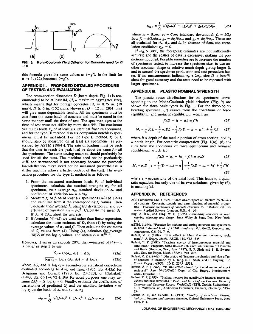
FIG. 9. Mohr-Coulomb Yield Criterion for Concrete used for 0 ~O
this formula gives the same values as (-g"). In the limit for n ~ 1, (22) becomes (-g").
APPENDIX II. PROPOSED DETAILED PROCEDURE OF TESTING AND EVALUATION
The cross-section dimension D (beam depth, Fig. 1) is recommended to be at least 8da (do = maximum aggregates size), which means that for normal concretes [do"'" 0.75 in. (19 mm)], D ~ 6 in. (152 mm). However, D = 12 in. (304 mm) will give more dependable results. All the specimens must be cast from the same batch of concrete and must be cured in the same manner until the time of test. The specimen ages at the time of test must not differ by more than 5%. The maximum (ultimate) loads P w of at least six identical fracture specimens, and for the type III method also six companion notchless specimens, must be measured. For the type II method, f; or.fr should also be measured on at least six specimens [as prescribed by ASTM (1994)]. The rate of loading must be such that the time to reach the peak load be about the same for all the specimens. The same testing machine should preferably be used for all the tests. The machine need not be particularly stiff, and servocontrol is not necessary because the postpeak load-deflection curve need not be measured (nevertheless, a stiffer machine allows a better control of the test). The evaluation procedure for the type II method is as follows:
1. From the measured maximum loads P w of individual specimens, calculate the nominal strengths erN for all specimen, their average aN, standard deviation SN, and coefficient of variation WN = sN/aN'
2. Measure f; or.fr on at least six specimens (ASTM 1994) and calculate from it the corresponding f: values. Then calculate their average J" standard deviation Sp, and coefficient of variation Wp = sp/J,. Calculate the mean ap. If ap :5 2aN' abort the analysis.
3. If formulas (4)-(5) are used rather than linear regression, calculate the mean estimate of Do from (4) by using the average values of erN andf:. Then calculate the estimates of G[ values from (4). Using (4), calculate the average log c[ of the log c[ values, and obtain c[ = 10108 c,.
However, if WN or Wp exceeds 20%, then-instead of (4)-it is better in step 3 to use
a[ = G[(aN' ap) + !1G[ (23a)
log c[ = log ciaN' ap) + !1 log c[ (23b)
where !1G[ and !1 log c[ = second-order statistical corrections evaluated according to Ang and Tang (1975, Eq. 4.43a) [or Benjamin and Cornell (1970, Eq. 2.4.123), or Elishakoff (1983, Eq. 6.91-6.92)]. But for most purposes one may assume !1G[ = !1 log cf = O. Finally, estimate the coefficients of variation W of predicted G[ and the standard deviation S of log c[ on the basis of SN and Sp, using
where SN = O'NWN; Sp = apWp (standard deviations); fN = aG/ aerN; fp = aG/aerp; gN = aC/aerN; and gp = ac/aerp. These are all evaluated for aN, ap, and cf' In absence of data, use correlation coefficient rNP "'" O.
If Wa > 30%, the foregoing estimates are not sufficiently accurat; and the scatter of data is excessive, making the predictions doubtful. Possible remedies are to increase the number of specimens tested, to increase the specimen size, to use another specimen shape or relative notch depth giving larger 13, and to control the specimen production and test procedure better. If the measurements indicate ap < 2aN' size D is insufficient for good accuracy and the tests need to be repeated with larger specimens.
APPENDIX III. PLASTIC NOMINAL STRENGTH
The plastic stress distributions for the specimens corresponding to the Mohr-Coulomb yield criterion (Fig. 9) are shown for three basic types in Fig. 1. For the three-poi ntbending specimen, (7) ensues from the conditions of force equilibrium and moment eqUilibrium, which are
f;(D - h - ao) =f:h (26)
M =1. P L = 1. er T\L = 1././(D - h - n.)2 + 1.f1h2
w 4 w 4J>L' 2 c -u 2' (27)
where h = depth of the tensile portion of cross section; and au = notch length. For eccentric compression [Fig. l(b)], (6) ensues from the conditions of force eqUilibrium and moment eqUilibrium, which are
(28)
[ 1 ] 1 I h 2 I 'h2 M. = er pi) e + 2: (D - ao) - h = 2: fAD - ao - ) + 2: it
(29)
where e = eccentricity of the axial load. This leads to a quadratic equation, but only one of its two solutions, given by (6), is meaningful.
APPENDIX IV. REFERENCES ACI Committee 446. (1992). "State-of-art-report on fracture mechanics
of concrete: Concepts, models and determination of material properties." Fracture mechanics of concrete structure, Z. P. Ba!ant, ed., Elsevier Applied Science, London, U.K., 4-144.
Ang, A. H-S., and Tang, W. H. (1975). Probability concepts in engi· neering planning and design. John Wiley & Sons, Inc., New York, N.Y.
ASTM. (1994). "Practice for making and curing concrete test specimens in field." Annual book of ASTM standards, Vol. 04.02, Concrete and Aggregates, C31-91, 7-9.
Balant, Z. P. (1984). "Size effect in blunt fracture: concrete, rock, metal." J. Engrg. Mech., ASCE, 110, 518-535.
Balant, Z. P. (1987). "Fracture energy of heterogeneous material and similitude." Preprints, SEM-RILEM Int. Conf. on Fracture of Concrete and Rock (Houston, Tex., June 1987), S. P. Shah and S. E. Swartz, eds., Soc. for Exper. Mech. (SEM), 390-402.
Balant, Z. P. (1994a). "Discussion of 'fracture mechanics and size effect of concrete in tension,' by T. Tang, S. P. Shah, and C. Ouyang." J. Struct. Engrg., ASCE, 120(8), 2555-2558.
Balant, Z. P. (1994b). "Is size effect caused by fractal nature of crack surfaces?" Rep. 94-10/C402i, Dept. of Civ. Engrg., Northwestern Univ., Evanston, Ill.
Balan!, Z. P. (1995). "Scaling theories for quasibrittle fracture: recent advances and new directions." Proc., 2nd Int. Con/. on Fracture Mech. of Concrete and Concrete Struct.,· FraMCoS2 (ETH, Zilrich, Switzerland), F. H. Wittmann, ed., Aedificatio Publishers, Freiburg, Germany, 515-534.
Balant, Z. P., and Cedolin, L. (1991). Stability of structures: Elastic. inelastic. fracture and damage theories, Oxford University Press. New York, N.Y.
JOURNAL OF ENGINEERING MECHANICS / MAY 1996/467
BaZant, Z. P., and Gettu, R. (1992). "Rate effects and load relaxation in static fracture of concrete." ACI Mat. J., 89-M49, Sept., 456-467.
BaZant, Z. P., Gettu, R., and Kazemi, M. T. (1991). "Identification of nonlinear fracture properties from size effect tests and structural analysis based on geometry-dependent R-curve." Int. J. Rock Mech. and Min. Sci., 28(1),43-51.
BaZant, Z. P., and Kazemi, M. T. (1990). "Determination of fracture energy, process zone length and brittleness number from size effect, with application to rock and concrete." Int. J. Fracture, 44, 111-131.
BaZant, Z. P., and Li, Z. (1995). "Modulus of rupture: Size effect due to fracture initiation in boundary layer." J. Straet. Engrg., ASCE, 121(4), 739-746.
BaZant, Z. P., Li, Z., and Li, Y.-N. (1994). "Brittle-plastic size effect method of measuring fracture properties of concrete or rock." Rep., Dept. of Civ. Engrg., Northwestern Univ., Evanston, Ill.
BaZant, Z. P., and Pfeiffer, P. A. (1987). "Determination of fracture energy from size effect and brittleness number." ACI Mat. J., 84(6), 463-480.
Benjamin, J. R., and Cornell, C. A. (1970). Probability, statistics, and decision for civil engineers. McGraw-Hill Book Co., New York, N.Y.
Broek, D. (1988). The practical use of fracture mechanics. Kluwer Academic Publishers, Dordrecht, The Netherlands.
Crow, E. L., Davis, F. A., and Maxfield, M. W. (1960). Statistics manual. Dover, New York, N.Y.
Elishakoff, I. (1983). Probability method in the theory of structures. John Wiley & Sons, Inc., New York, N.Y.
4681 JOURNAL OF ENGINEERING MECHANICS 1 MAY 1996
Gettu, R., BaZant, z. P., and Karr, M. E. (1990). "Fracture properties and brittleness of high strength concrete." ACI Mat. J., 87-M66, Nov., 608-618.
Hillerborg, A. (1985). "Results of three comparative test series for determining the fracture energy G, of concrete." Mat. and Struct., Paris, France, 18(107),407-413.
Jenq, Y. S., and Shah, S. P. (1985). "A two parameter fracture model for concrete." J. Engrg. Mech., ASCE, 111(4), 1227-1241.
Kanninen, M. F., and Popeiar, C. H. (1985). Advancedfracture mechanics. Oxford University Press, New York, N.Y.
Planas, J., and Elices, M. (1989). "Size effect in concrete structures: Mathematical approximations and experimental validation." Cracking and damage: Strain localization and size effect, J. Mazars and Z. P. BaZant, eds., Elsevier, London, U.K., 462-476.
RILEM Recommendation. (1990). "Size effect method for determining fracture energy and process zone of concrete." Mat. and Struct., Paris, France, 23, 461-465.
Tada, H., Paris, P., and Irwin, G. (1985). The stress analysis of cracks handbook, 2nd Ed., Paris Productions Inc., Mo.
Tang, T., Batant, Z., Yang, S., and Zollinger, D. (1995). "Variable-notch one-size test method for fracture energy and process zone length." Engrg. Fracture Mech.
Wells, A. A. (1961). "Unstable crack propagation in metals-cleavage and fast fracture." Symp. on Crack Propagation, Cranfield, U.K., 1,210-230.