(c) 2004 F. Estrada & A. Jepson & D. Fleet Local Features ...jepson/csc2503/tutSIFT04.pdfLocal...

(c) 2004 F. Estrada & A. Jepson & D. Fleet

Local Features Tutorial: Nov. 8, ’04

Local Features Tutorial

References:

• Matlab SIFT tutorial (from course webpage)

• Lowe, David G. ’Distinctive Image Features fromScale Invariant Features’, International Journal ofComputer Vision, Vol. 60, No. 2, 2004, pp. 91-110

Local Features Tutorial 1



Previous week: View based models for object

recognition

- The problem: Build a model that captures general

properties of eye appearance that we can use to identifyeyes (though the approach is general, and does notdepend on the particular object class).

- Generalized model of eye appearance based on PCA.Images taken from same pose and normalized forcontrast.

- Demonstrated to be useful for classification, keyproperty: the model can find instances of eyes it hasnever seen before.




Today: Local features for object recognition

- The problem: Obtain a representation that allowsus to find a particular object we’ve encountered before(i.e. “find Paco’s mug” as opposed to “find a mug”).

- Local features based on the appearance of the objectat particular interest points.

- Features should be reasonably invariant toillumination changes, and ideally, also to scaling,rotation, and minor changes in viewing direction.

- In addition, we can use local features for matching,this is useful for tracking and 3D scene reconstruction.




Key properties of a good local feature:

- Must be highly distinctive, a good feature shouldallow for correct object identification with lowprobability of mismatch. Question: How to identify

image locations that are distinctive enough?.

- Should be easy to extract.

- Invariance, a good local feature should be tolerant to� Image noise� Changes in illumination� Uniform scaling� Rotation� Minor changes in viewing directionQuestion: How to construct the local feature to

achieve invariance to the above?

- Should be easy to match against a (large) databaseof local features.



SIFT features

Scale Invariant Feature Transform (SIFT) is anapproach for detecting and extracting local featuredescriptors that are reasonably invariant to changes inillumination, image noise, rotation, scaling, and smallchanges in viewpoint.

Detection stages for SIFT features:

- Scale-space extrema detection

- Keypoint localization

- Orientation assignment

- Generation of keypoint descriptors.

In the following pages we’ll examine these stages indetail.

SIFT features 5


Scale-space extrema detection

Interest points for SIFT features correspond to localextrema of difference-of-Gaussian filters at differentscales.

Given a Gaussian-blurred image

L(x, y, σ) = G(x, y, σ) ∗ I(x, y),

where

G(x, y, σ) = 1/(2πσ2) exp−(x2+y2)/σ2

is a variable scale Gaussian, the result of convolving animage with a difference-of-Gaussian filter

G(x, y, kσ) − G(x, y, σ)

is given by

D(x, y, σ) = L(x, y, kσ) − L(x, y, σ) (1)

Scale-space extrema detection 6


Which is just the difference of the Gaussian-blurredimages at scales σ and kσ.

Figure 1: Diagram showing the blurred images at different

scales, and the computation of the difference-of-Gaussian images

(from Lowe, 2004, see ref. at the beginning of the tutorial)

The first step toward the detection of interest pointsis the convolution of the image with Gaussian filtersat different scales, and the generation of difference-of-Gaussian images from the difference of adjacent blurredimages.




The convolved images are grouped by octave (anoctave corresponds to doubling the value of σ), and thevalue of k is selected so that we obtain a fixed numberof blurred images per octave. This also ensures thatwe obtain the same number of difference-of-Gaussianimages per octave.

Note: The difference-of-Gaussian filter provides anapproximation to the scale-normalized Laplacian ofGaussian σ2

∇2G. The difference-of-Gaussian filter is

in effect a tunable bandpass filter.




Figure 2: Local extrema detection, the pixel marked × is

compared against its 26 neighbors in a 3 × 3 × 3 neighborhood

that spans adjacent DoG images (from Lowe, 2004)

Interest points (called keypoints in the SIFTframework) are identified as local maxima or minimaof the DoG images across scales. Each pixel in theDoG images is compared to its 8 neighbors at thesame scale, plus the 9 corresponding neighbors atneighboring scales. If the pixel is a local maximum orminimum, it is selected as a candidate keypoint.




For each candidate keypoint:

- Interpolation of nearby data is used to accuratelydetermine its position.

- Keypoints with low contrast are removed

- Responses along edges are eliminated

- The keypoint is assigned an orientation

To determine the keypoint orientation, a gradientorientation histogram is computed in the neighborhoodof the keypoint (using the Gaussian image at the closestscale to the keypoint’s scale). The contribution of eachneighboring pixel is weighted by the gradient magnitudeand a Gaussian window with a σ that is 1.5 times thescale of the keypoint.

Peaks in the histogram correspond to dominantorientations. A separate keypoint is created for thedirection corresponding to the histogram maximum,



and any other direction within 80% of the maximumvalue.

All the properties of the keypoint are measured relativeto the keypoint orientation, this provides invariance torotation.



SIFT feature representation

Once a keypoint orientation has been selected, thefeature descriptor is computed as a set of orientationhistograms on 4 × 4 pixel neighborhoods. Theorientation histograms are relative to the keypointorientation, the orientation data comes from theGaussian image closest in scale to the keypoint’s scale.

Just like before, the contribution of each pixel isweighted by the gradient magnitude, and by a Gaussianwith σ 1.5 times the scale of the keypoint.

Figure 3: SIFT feature descriptor (from Lowe, 2004)

SIFT feature representation 12


Histograms contain 8 bins each, and each descriptorcontains an array of 4 histograms around the keypoint.This leads to a SIFT feature vector with 4 × 4 × 8 =128 elements. This vector is normalized to enhanceinvariance to changes in illumination.

SIFT feature representation 13


SIFT feature matching

- Find nearest neighbor in a database of SIFT featuresfrom training images.

- For robustness, use ratio of nearest neighbor to ratioof second nearest neighbor.

- Neighbor with minimum Euclidean distance →

expensive search.

- Use an approximate, fast method to find nearestneighbor with high probability.

SIFT feature matching 14


Recognition using SIFT features

- Compute SIFT features on the input image

- Match these features to the SIFT feature database

- Each keypoint specifies 4 parameters: 2D location,scale, and orientation.

- To increase recognition robustness: Hough transformto identify clusters of matches that vote for the sameobject pose.

- Each keypoint votes for the set of object poses thatare consistent with the keypoint’s location, scale, andorientation.

- Locations in the Hough accumulator that accumulateat least 3 votes are selected as candidate object/posematches.

- A verification step matches the training image forthe hypothesized object/pose to the image using aleast-squares fit to the hypothesized location, scale,and orientation of the object.

Recognition using SIFT features 15


SIFT matlab tutorial

Gaussian blurred images and Difference of Gaussianimages

Range: [−0.11, 0.131] Dims: [959, 2044]

Figure 4: Gaussian and DoG images grouped by octave

SIFT matlab tutorial 16



Keypoint detection

a)

c)

b)

Figure 5: a) Maxima of DoG across scales. b) Remaining

keypoints after removal of low contrast points. C) Remaining

keypoints after removal of edge responses (bottom).




Final keypoints with selected orientation and scale

Figure 6: Extracted keypoints, arrows indicate scale and

orientation.




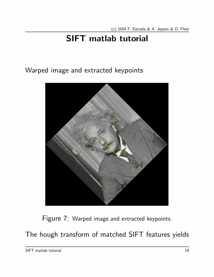
Warped image and extracted keypoints

Figure 7: Warped image and extracted keypoints.

The hough transform of matched SIFT features yields



the transformation that aligns the original and warpedimages:

Computed affine transformation from rotated image to

original image:

>> disp(aff);

0.7060 -0.7052 128.4230

0.7057 0.7100 -128.9491

0 0 1.0000

Actual transformation from rotated image to

original image:

>> disp(A);

0.7071 -0.7071 128.6934

0.7071 0.7071 -128.6934

0 0 1.0000




Matching and alignment of different views using localfeatures.

Orignial View

Range: [0, 1] Dims: [384, 512]

Reference View

Range: [0, 1] Dims: [384, 512]

Aligned View

Range: [−0.0273, 1] Dims: [384, 512]

Reference minus Aligned View

Range: [−0.767, 0.822] Dims: [384, 512]

Figure 8: Two views of Wadham College and affine

transformation for alignment.




Object recognition with SIFT

Image

Range: [0, 1] Dims: [480, 640]

Model

Range: [0, 1] Dims: [480, 640]

Location

Range: [−0.986, 0.765] Dims: [480, 640]

Image

Range: [0, 1] Dims: [480, 640]

Model

Range: [0, 1] Dims: [480, 640]

Location

Range: [−1.05, 0.866] Dims: [480, 640]

Image

Range: [0, 1] Dims: [480, 640]

Model

Range: [0, 1] Dims: [480, 640]

Location

Range: [−1.07, 1.01] Dims: [480, 640]

Figure 9: Cellphone examples with different poses and occlusion.




Object recognition with SIFT

Image

Range: [0, 1] Dims: [480, 640]

Model

Range: [0, 1] Dims: [480, 640]

Location

Range: [−0.991, 0.992] Dims: [480, 640]

Image

Range: [0, 1] Dims: [480, 640]

Model

Range: [0, 1] Dims: [480, 640]

Location

Range: [−1.05, 0.963] Dims: [480, 640]

Image

Range: [0, 1] Dims: [480, 640]

Model

Range: [0, 1] Dims: [480, 640]

Location

Range: [−0.988, 1.05] Dims: [480, 640]

Figure 10: Book example, what happens when we match similar

features outside the object?



Closing Comments

- SIFT features are reasonably invariant to rotation,scaling, and illumination changes.

- We can use them for matching and object recognitionamong other things.

- Robust to occlusion, as long as we can see at least 3features from the object we can compute the locationand pose.

- Efficient on-line matching, recognition can beperformed in close-to-real time (at least for small objectdatabases).

Closing Comments 24


Closing Comments

Questions:

- Do local features solve the object recognitionproblem?

- How about distinctiveness? how do we deal with falsepositives outside the object of interest? (see Figure10).

- Can we learn new object models withoutphotographing them under special conditions?

- How does this approach compare to the objectrecognition method proposed by Murase and Nayar?Recall that their model consists of a PCA basisfor each object, generated from images taken underdiverse illumination and viewing directions; and arepresentation of the manifold described by the trainingimages in this eigenspace (see the tutorial on EigenEyes).

Closing Comments 25

Date post:	28-Apr-2018
Category:	Documents
Upload:	haque
View:	217 times
Download:	3 times

(c) 2004 F. Estrada & A. Jepson & D. Fleet Local Features ...jepson/csc2503/tutSIFT04.pdfLocal...

Documents