THERMAL TRANSPORT IN NANOSTRUCTURED MATERIALS By CHIA-YI CHEN A DISSERTATION PRESENTED TO THE GRADUATE SCHOOL OF THE UNIVERSITY OF FLORIDA IN PARTIAL FULFILLMENT OF THE REQUIREMENTS FOR THE DEGREE OF DOCTOR OF PHILOSOPHY UNIVERSITY OF FLORIDA 2008 1
Transcript
THERMAL TRANSPORT IN NANOSTRUCTURED MATERIALS
By
CHIA-YI CHEN
A DISSERTATION PRESENTED TO THE GRADUATE SCHOOLOF THE UNIVERSITY OF FLORIDA IN PARTIAL FULFILLMENT
OF THE REQUIREMENTS FOR THE DEGREE OFDOCTOR OF PHILOSOPHY
3-1 Local energy evolution and detail of breather interaction in a FPU chain usingthe protocol of Reigada et al.[38] for k = β = 1/2, α = 0. . . . . . . . . . . . . . 25
3-2 Floquet multipliesr and the effect of unstable perturbation of breather solutions. 28
3-3 Families of breathers with different configurations. . . . . . . . . . . . . . . . . . 28
3-4 A family of breather solutions with ST mode configuration and their stabilityanalysis for a FPU-α system. . . . . . . . . . . . . . . . . . . . . . . . . . . . . 29
3-5 Results of the stability analysis of the ST mode breathers for a range of α, ω,and fixed β = 1. . . . . . . . . . . . . . . . . . . . . . . . . . . . . . . . . . . . . 30
3-6 Nonlinear vibration mode and its stability analysis for a single FPU chain intwo-dimensional system. . . . . . . . . . . . . . . . . . . . . . . . . . . . . . . . 32
3-7 The configuration for two coupled FPU chains. . . . . . . . . . . . . . . . . . . 33
3-8 Nonlinear vibration mode and its stability analysis for two coupled FPU chainsin two-dimensional system with kFPU = kcoupling = 1, α = β = 0. . . . . . . . . . 33
3-9 Nonlinear vibration mode and its stability analysis for two coupled FPU chainsin two-dimensional system with (kFPU , kcoupling, βFPU) = (1, 1, 1). . . . . . . . . . 34
3-10 The configuration for body-centered cubic structure system. . . . . . . . . . . . 34
3-11 Continuation curves and configuration of nonlinear solutions corresponding todifferent amplitudes of the phonon modes. . . . . . . . . . . . . . . . . . . . . . 36
3-13 Structure of a unit cell of the model hexagonal system in three dimensions. . . . 38
3-14 The dispersion curves for three-dimensional hexagonal tube system. . . . . . . 39
3-15 One of the phonon modes of the hexagonal system and its stability analysis with(k,β)coupling/FPU = (1, 0). . . . . . . . . . . . . . . . . . . . . . . . . . . . . . . . 40
3-16 Initial guess for the Newton’s method for 3D hexagonal system. . . . . . . . . . 41
3-17 Dependence of amplitude and frequency of a steady-state mode on the strengthof coupling between chains in hexagonal system. . . . . . . . . . . . . . . . . . . 41
3-18 Configuration of the nonlinear solutions with (k, β)coupling = (1, 1). . . . . . . . . 42
3-19 The comparison of solutions with and without RWA. . . . . . . . . . . . . . . . 43
9
3-20 Comparison of nonlinear modes of hexagonal system for three different couplingstrength. . . . . . . . . . . . . . . . . . . . . . . . . . . . . . . . . . . . . . . . . 43
4-1 Preparation of a nanotube by rolling the graphite sheet in a direction specifiedby the chiral vector Ch . . . . . . . . . . . . . . . . . . . . . . . . . . . . . . . . 48
4-2 Comparison of ratio of the magnitude of the nonlinear and linear force of CNTand FPU system . . . . . . . . . . . . . . . . . . . . . . . . . . . . . . . . . . . 50
4-3 Temperature profile and local energy evolution of NEMD simulations of a segmentof a 100 unit-cell (5,0) CNT. . . . . . . . . . . . . . . . . . . . . . . . . . . . . . 52
4-5 The summary of the numerical procedure to obtain Fourier series expansion fora complex potential. . . . . . . . . . . . . . . . . . . . . . . . . . . . . . . . . . 54
4-6 Comparison between a linear phonon mode of the (5,0) carbon nanotube andthe nonlinear mode obtained from this mode by the continuation method. . . . 56
4-7 Dependence of the mode energy and frequency of the Taylor solutions on ε forsolutions shown in Figure 4-6. . . . . . . . . . . . . . . . . . . . . . . . . . . . . 57
4-8 The solutions of (5,0) CNT in two unit cells system starting with the amplitudecorresponding to three different temperature. . . . . . . . . . . . . . . . . . . . 58
4-9 Dependence of the mode energy and frequency of the Taylor solutions startingwith three initial thermal energy on ε for solutions shown in figure 4-8. . . . . . 59
4-10 The comparison the displacement for the 7th atom in each unit cell for ε = 1nonlinear mode and starting phonon mode in a 24 unit cells system with thesimplified potential under RWA approximation. . . . . . . . . . . . . . . . . . . 60
4-11 The nonlinear vibration modes with simplified potential for the systems up to24 unit cells. . . . . . . . . . . . . . . . . . . . . . . . . . . . . . . . . . . . . . . 61
4-12 Configuration of a linearly stable nonlinear solution based on simplified potentialfunction for a four unit cells system. . . . . . . . . . . . . . . . . . . . . . . . . 61
4-13 The nonlinear solution based on simplified potential function for a four unit cellssystem. . . . . . . . . . . . . . . . . . . . . . . . . . . . . . . . . . . . . . . . . 62
4-14 The eigenvector corresponding the Floquet multiplier shown as the open circlein Figure 4-13B. . . . . . . . . . . . . . . . . . . . . . . . . . . . . . . . . . . . 62
10
5-1 A block of 2× 2× 2 sodalite unit cells containing nine sodalite cages. . . . . . . 66
Abstract of Dissertation Presented to the Graduate Schoolof the University of Florida in Partial Fulfillment of theRequirements for the Degree of Doctor of Philosophy
THERMAL TRANSPORT IN NANOSTRUCTURED MATERIALS
By
Chia-Yi Chen
August 2008
Chair: Dmitry I. KopelevichMajor: Chemical Engineering
Thermal transport in nanostructured materials often exhibits significant deviations
from predictions of the classical Fourier’s law for thermal conductivity. The deviations
occur because the length of the mean free path of heat-carrying phonons is comparable
with characteristic length-scale of these materials. Therefore, it is necessary to develop
a theory for thermal transport applicable to nanomaterials. In this study we investigate
thermal conductivity in two classes of nanomaterials, namely quasi-one-dimensional
materials and nanoporous materials with adsorbed guest molecules. For quasi-one-
dimensional (Q1D) materials, we aim to understand nonlinear dynamics involved in heat
transfer using a combination of molecular dynamics simulations and bifurcation theory.
In non-equilibrium molecular dynamics simulations, we observe ballistic propagation of
energy packets in model Q1D systems as well as in carbon nanotubes, which suggests
the significance of ballistic heat transfer mechanism. To decipher structure of the
waves propagating in the lattice, we obtain nonlinear lattice vibration modes by solving
fundamental equations of motion numerically, without ignoring any structural details. We
focus on localized nonlinear vibration modes, and investigate their properties and stability
on the structured details of the lattice, and potential energy of interaction between lattice
atoms.
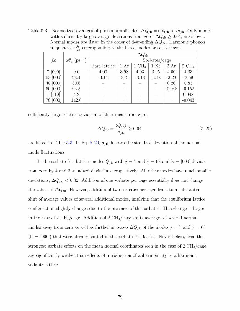
In the second part of this work, we investigate the effect of sorbate-lattice interaction
in thermal transport for nanoporous materials. There is increasing evidence that thermal
13
conductivity of nanoporous materials can be significantly affected by adsorption of guest
molecules. These molecules serve as moving defects and provide additional scattering
centers for heat-carrying phonons. In order to understand the sorbate-phonon interactions,
we first perform molecular dynamics simulations of a realistic system, namely sodalite
zeolite with small molecules (argon, xenon, and methane) encapsulated in its cages.
We observe that the phonon lifetime often increases upon encapsulation of a sorbate
into the zeolite which suggests that the sorbate-phonon interactions are qualitatively
different from phonon scattering by point defects fixed in the lattice. We then proceed
to develop a model for the sorbate-lattice interaction. For simplicity, we consider a one-
dimensional lattice system. We investigate the role of the sorbate in the energy exchange
between lattice modes and observe that even a weak interaction between the sorbate and
lattice induces dispersion of energy over a wide spectrum of normal modes.
14
CHAPTER 1INTRODUCTION
Advances in materials science and manufacturing technology have enabled integration
of nanostructured materials in electronics, energy conversion systems and sensors. For
example, it is believed that CMOS (complementary metal-oxide semiconductor) will
decrease to 22-nm within next 10 years [1]. To improve footprint of elements of integrated
circuits, non-volatile memory devices using 1D structures such as nanowires and nanotubes
have drawn significant attention. In order to ensure the performance and stability of
incandesces, it is necessary to assess thermal properties of new nanoscale materials [2, 3].
The classical Fourier’s law of thermal conductivity, states that the heat flux J is linearly
proportional to the temperature gradient ∇T ,
J = −κ∇T, (1–1)
where the thermal conductivity κ can be approximated as [4]:
κ ∝ Cvl. (1–2)
Here, C, v, and l are the heat capacity, the group velocity and the mean free path of the
phonons respectively. The assumptions behind equations (1–1) and (1–2) are that (i)
the phonon mean free path l is much smaller than the characteristic size of the material
and (ii) the temperature gradient is sufficiently small so that collisions between phonons
maintain local equilibrium.
Both of these assumptions are likely to fail in nanosomia systems. For example, the
mean free path of heat-carrying phonons in silicon at 300 K is 300 nm whereas the current
dimension of a thin silicon film is under 100 nm [2] and the characteristic size of a hotspot
in a transistor can be as small as 10 nm [5]. Therefore, it is necessary to consider the
effect of boundary scattering and phonon confinement [6–8] explicitly. These issues are
15
currently being addressed by development and solution of the Boltzmann equation for the
phonon scattering due to phonon-phonon and phonon-boundary interactions.
The second assumption is also likely to fail in nanosomia materials, where thermal
gradients can be significant. In this case, the Boltzmann equation for phonon modes might
be invalid since the role of nonlinearities of the lattice vibration will not be limited to
energy exchange during collisions of linear phonon modes. In fact, recent investigations
have shown that different type of lattice vibration modes, known as the intrinsic nonlinear
localized modes or breathers [9–11], make a strong contribution to the thermal energy
transfer and lead to qualitatively different thermal properties in low dimensional materials.
In fact, it has been shown both theoretically, using the self-consistent mode coupling
theory [12, 13], and by numerical simulations [13–15] that the bulk heat conductivity
exhibits anomalous dependence on the lattice size for one- and two-dimensional lattices.
In the current work, we investigate the process of thermal conductivity in one- and
quasi-one-dimensional systems such as carbon nanotubes (CNTs) [16]. Due to their
unique mechanical and electronic properties, CNTs have drawn significant attention
for a wide variety of potential applications, [17] and are currently being integrated into
electronic devices such as high-performance ballistic field-effect transistors, nanotube
random access memory (NRAM) and assembling integrated logic circuit on an individual
carbon nanotube [18–20]. Currently there is only incomplete understanding regarding
thermal transport for CNTs, which is extremely important for heat management issue.
of Eq. 2–2; the period of this solution is T = 2π/ω. For convenience, let us rewrite the
equations of motion Eq. 2–2 as a first-order system of equations,
Yn(t) = fn(t), (2–21)
22
where
fn(t) = un(t) = YN+n(t), n = 1, . . . , N, (2–22)
fN+n(t) = un(t) = − ∂V
∂Yn
, n = 1, . . . , N. (2–23)
Now consider a perturbation of Y(0)(t) of the form Y(t) = Y(0)(t) + εY(1)(t), ε ¿ 1. The
equations linearized near the steady-state solution are
Y(1)n =
∑m
Lnm(Y(0)(t))Y(1)m , n = 1, . . . 2N, (2–24)
where the time-periodic d× d matrices Lnm are given by
Lnm(Y(0)) =∂fn(Y(0))
∂Y(0)m
. (2–25)
In order to apply the Floquet analysis, we obtain a 2Nd × 2Nd matrix F (t) of
fundamental solutions of the linearized equations (2–24). The j-th column of this matrix
corresponds to the solution with the initial condition of the form Y(1,j)(t = 0) =
(0, 0, . . . , 0, 1, 0, . . . , 0) with the only non-zero element of the vector Y(1,j)(t = 0) located
at the j-th position. These solutions are obtained by the numerical integration of the
system of linearized equations (2–24). Once the fundamental solutions are obtained, we
compute the Floquet multipliers, i.e. the eigenvalues µj (j = 1, . . . , 2Nd) of the matrix
F (t) at time t = T . The steady-state solution is stable only if all of the Floquet multipliers
have magnitude less than or equal to 1. Since the system considered in this work is
Hamiltonian, for each eigenvalue µj the numbers µ∗j and 1/µj are also eigenvalues [11]
(here, asterisk denotes complex conjugation). Thus the neutral stability of the steady-state
solution requires that all the multipliers lie on the unit circle of the complex plane.
23
CHAPTER 3NONLINEAR LATTICE VIBRATION MODES IN MODEL SYSTEMS
3.1 One-Dimensional FPU system
In this section, we illustrate the methods employed in this work by application to a
one-dimensional Fermi-Pasta-Ulam (FPU) [36] system, i.e. a linear anharmonic chain of
atoms with the following Hamiltonian:
H =∑
n
[u2
n
2+
k
2(un − un−1)
2 +α
3(un − un−1)
3 +β
4(un − un−1)
4
]. (3–1)
Here, un is the mass-normalized displacement of the n-th atom from its equilibrium
position and k, α, and β are the harmonic, cubic, and quartic force constants, respectively.
The considered chain consists of N = 50 atoms with imposed periodic boundary
conditions, i.e. u1 = uN+1 and u1 = uN+1. In the analysis of the FPU system, we fix
the value of the harmonic spring constant k = 1 and vary the anharmonic spring constants
α and β. In literature, the system with α = 0 is referred to as FPU-β model and the
system with α 6= 0 is referred to as FPU-α model.
3.1.1 Thermal Relaxation Simulation
It has been shown in the literature that in addition to phonons, energy in FPU
system may be transmitted by intrinsic localized modes, also known as discrete breathers
(DBs) [9, 11, 37], DBs are intrinsic localized nonlinear vibration modes that are
qualitatively different from the phonon modes and can be observed in thermal relaxation
of the lattice. MD simulations of thermal relaxation of FPU system have been performed
by Reigada et al. [38]. They prepared a 30-site lattice initially thermalized at T = 0.5
by Langevin thermostat and after the system reached equilibrium, they disconnected the
thermalized lattice system from the heat bath and connected the ends of the chain via a
friction term γ to dissipate the energy into the thermal reservoir of zero temperature. Here
we show the results of our simulations following their protocol for a N = 50 lattice with
k = β = 1/2, α = 0. The evolution of the local energy of this system during relaxation
24
A B
10 20 30 40 50−0.5
0
0.5
Atom
Dis
plac
emen
t
Time=1754.5
C
10 20 30 40 50−0.5
0
0.5
Atom
Dis
plac
emen
t
Time=1809.5
D
10 20 30 40 50−0.5
0
0.5
AtomD
ispl
acem
ent
Time=1846.5
E
Figure 3-1. (A) The breathers in a FPU chain obtained using the protocol of Reigada etal.[38] for k = β = 1/2, α = 0. The gray scale in this figure represents the localenergy magnitude, with darker shading corresponding to more energeticregions. The horizontal axis indicates the position along the chain and thevertical axis corresponds to time. The energy density is shown by a gray scalefrom 0 (white) to the maximum energy recorded during the simulation (black).The energy localizes into narrow breathers which are seen as the black lines onthis plot. The noisy phonon modes correspond to randomly shaded areas. B),Details of the energy localization and breather interaction. C), D) and E) aresnapshots for the process of breather-breather corresponding to three differenttimes in relaxation simulation indicated by the dashed lines in plot B.
process is plotted in Figure 3-1 A), where the darker region represents higher energy. We
observe the ballistic energy transfer clearly after the dissipations of phonon modes.
The breathers are seen to move with essentially constant speed and appear to be
stable with respect to the low-energy noisy phonon modes. Details of breather-breather
interactions are shown in plot B and snapshots for this process are shown in plots C-E.
25
Elastic interaction is observed between breathers. It is clear that, after initial transient,
the energy becomes highly localized and in addition to phonons, the system contains
localized nonlinear structures (breathers).
3.1.2 Steady State Solutions
Steady-state solutions are approximated by rotating wave approximation (RWA) [39],
in which coefficients with j ≥ 2 in Eq. 2–15 are neglected. Therefore, the nonlinear terms
in the equations of motion are approximated as follows:
cos2(ωt) ' 12, cos3(ωt) ' 3
4cos(ωt) (3–2)
We compare each of the Fourier coefficients in Eq. 2–2 to set up the equations for
Newton’s method. Since quadratic force term is approximated by a constant under
RWA approximation, it leads to non-zero average displacements xn,0 of atoms.
3.1.2.1 FPU-β model
In this case, there is no quadratic nonlinear force and we seek the solution only with
j = 1 term:
un = xncos(ωt) (3–3)
Based on the solution configuration and the researchers who proposed the analytical
solution form of nonlinear solutions, DBs with asymmetric configuration in Figure 3-3 A)
(lower inset plot) is referred to as P mode (abbreviation for Page [40]). The DBs with
symmetric configuration in the lower inset plot of Figure 3-3 B) are referred to as ST
mode (abbreviation for Sievers and Takeno [41]). The initial guess for Newton’s method
are two of the high frequency phonon modes with wave vector k ≈ πa, shown in the
upper insets in Figure 3-3 A) and Figure 3-3 B). We perform continuation of solution by
gradually increasing β and ω by ∆β = 0.05 and ∆ω = 3× 10⁻³ until β = 1. The frequency
of DBs should be outside of the phonon frequency band to avoid resonance with phonon
solutions [9]. These two degenerate normal modes lead to two family of P mode and ST
mode breathers. The dependence of the mode energy on β are shown in Figure 3-3. Linear
26
stability of the breather modes to perturbations is examined using the Floquet analysis
described in Section 2.4. Recall that a vibration mode is stable only if all of its Floquet
multipliers µj lie on the unit circle of the complex plane. The closed and open circles
in these two figures represent the stable and unstable solutions, respectively. Results of
Floquet analysis for a stable ST mode DB with β = 1 is shown in Figure 3-2 A), where
µj are located on the unit circle. However, P modes are linearly unstable with unstable
multipliers being pure real numbers as shown in Figure 3-2 B). Figure 3-2 C) shows the
eigenvector corresponding to multiplier indicated by an open circle in Figure 3-2 B). In
order to understand the effect of this perturbation vector, we perform MD simulation with
initial condition as P mode breather with perturbation vector. Two snapshots are shown
in plot D and E. Initially, this perturbation results in the DB moving to the right and
eventually leading to a transition between P mode and ST mode configurations.
3.1.2.2 FPU-α model
In order to assess the role of the cubic term in Hamiltonian (Eq. 2–2), we turn to
the FPU-α model. We seek solutions with the RWA approximation, Eq. 3–2. Now, the
solutions will contain a static component,
un = xn,0 + xn,1cos(ωt). (3–4)
We take the DBs of the FPU-β systems as an initial guess for Newton’s method and
increase the cubic coefficient α. An example of an obtained steady-state P mode is shown
in Figure 3-4 A). We observe that the breather amplitude A increases with increase of the
magnitude of the cubic nonlinearity α. The dependence of A on α for a fixed frequency
ω = 2.89 and quartic term β = 1 is shown in Figure 3-4 B). We obtained breather families
for a range of ω between 2.2 and 2.93 (while keeping β = 1), and observed the increasing
of A while increasing α value as well. Interestingly, we observe that introduction of the
cubic nonlinearity destabilizes the breather modes. The stable and unstable breathers are
shown respectively by solid and open circles in Figure 3-4 B). To summarize the results of
27
−1 0 1
−1
0
1
Re(µ)
Im(µ
)
A
−1 0 1
−1
0
1
Re(µ)
Im(µ
)
B
20 30
−0.5
0
0.5
Particle Position
Dis
plac
emen
t
DBe
x
ev
C
10 20 30 40 50
−0.6
0
0.6
Time=0.025
Atom
Dis
plac
emen
t
D
10 20 30 40 50
−0.6
0
0.6
Time=2.2
Atom
Dis
plac
emen
t
E
Figure 3-2. Floquet multipliers DBs: A) ST mode and B) P mode solutions. (C) shows theDB configuration as well as the unstable displacement (ex) and velocity (ev)perturbation corresponding to the open circle in plot B The snapshots of MDsimulations for perturbed P mode breathers. (D) Initial configuration (E)shows the transition from P mode to ST mode.
0 0.2 0.4 0.6 0.8 1
1
2
3
4
5
6
7
β
Ene
rgy
−0.3
0
0.3β = 0
−0.8
0
0.8β = 1
A
0 0.2 0.4 0.6 0.8 1
1
2
3
4
5
6
7
β
Ene
rgy
−0.3
0
0.3β = 0
−0.8
0
0.8β = 1
B
Figure 3-3. Two family of (A) ST modes and (B) P mode DBs. The closed (open) circlesrepresent the linearly stable (unstable) modes.
28
10 20 30 40 50−0.8
−0.4
0
0.4
0.8ω=2.87, β=1, α=0.2
n, atom number
Xn,
j
Static (j=0)Dynamic (j=1)
A
0 0.2 0.4 0.6 0.8 10.38
0.4
0.42
0.44
0.46
0.48
0.5
0.52
α
A
ω=2.3061, β = 1
−1 1−1
1
α = 0.24
−1 1−1
1
α = 0.78
B
0 0.2 0.4 0.6 0.8 1
0.8
0.85
0.9
α
A
0 0.2 0.4 0.6 0.8 10
0.01
0.02
α
ν
C
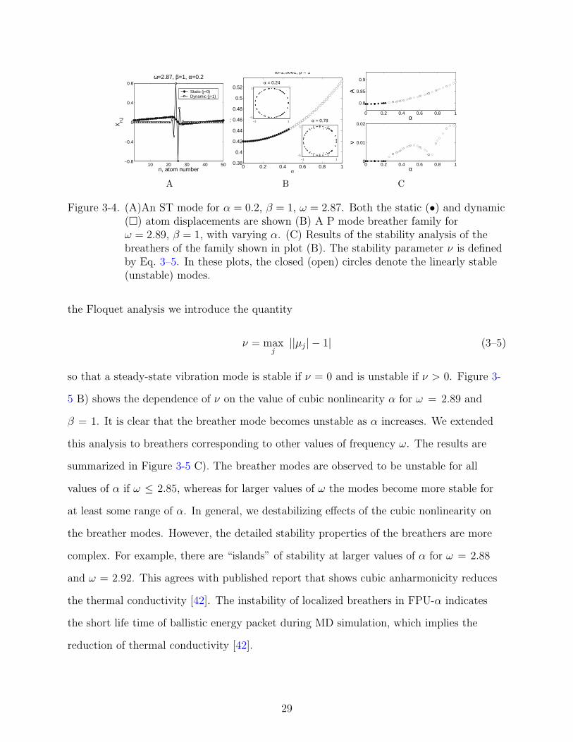
Figure 3-4. (A)An ST mode for α = 0.2, β = 1, ω = 2.87. Both the static (•) and dynamic(¤) atom displacements are shown (B) A P mode breather family forω = 2.89, β = 1, with varying α. (C) Results of the stability analysis of thebreathers of the family shown in plot (B). The stability parameter ν is definedby Eq. 3–5. In these plots, the closed (open) circles denote the linearly stable(unstable) modes.
the Floquet analysis we introduce the quantity
ν = maxj
||µj| − 1| (3–5)
so that a steady-state vibration mode is stable if ν = 0 and is unstable if ν > 0. Figure 3-
5 B) shows the dependence of ν on the value of cubic nonlinearity α for ω = 2.89 and
β = 1. It is clear that the breather mode becomes unstable as α increases. We extended
this analysis to breathers corresponding to other values of frequency ω. The results are
summarized in Figure 3-5 C). The breather modes are observed to be unstable for all
values of α if ω ≤ 2.85, whereas for larger values of ω the modes become more stable for
at least some range of α. In general, we destabilizing effects of the cubic nonlinearity on
the breather modes. However, the detailed stability properties of the breathers are more
complex. For example, there are “islands” of stability at larger values of α for ω = 2.88
and ω = 2.92. This agrees with published report that shows cubic anharmonicity reduces
the thermal conductivity [42]. The instability of localized breathers in FPU-α indicates
the short life time of ballistic energy packet during MD simulation, which implies the
reduction of thermal conductivity [42].
29
0 0.2 0.4 0.6 0.8 1
2.84
2.88
2.92
α
ω
Figure 3-5. Results of the stability analysis of the ST mode breathers for a range of α, ω,and fixed β = 1. The closed (open) circles denote the stable (unstable) modes.
3.2 Lattice Model Systems In Higher Dimensions
Breathers in one-dimensional model lattices have been studied both theoretically and
numerically [10, 43–53]. The breathers have also been observed in models of real physical
system, such as a molecular model for a row of atoms in a semiconductor crystal GaN
[54]. In addition to periodic atomic chains, breathers have been observed in simulations of
disordered systems [44, 55], which has important implications for thermal conductivity in
polymers and biological systems. Moreover, several experimental studies indicate existence
of breathers in molecular systems. For example, spectroscopic studies of laser-induced
vibrations in a quasi-one-dimensional chain of halogen-bridged mixed Pt complex [56, 57]
report a Raman spectrum characteristic of localized nonlinear vibration modes. The
intrinsic localized modes have also been experimentally observed in myoglobin [58].
In the previous section we discussed FPU model with atoms allowed to move only
along the chain. It is more realistic to allow vibrations in more than one direction and
so below we investigate the existence and stability analysis for nonlinear lattice vibration
modes in two and three-dimensional lattice systems with high aspect ratio. We perform
the numerical calculation for few different model systems: a single FPU chain in two-
dimensional system; two coupled FPU chains in two dimensional system, body-centered
cubic structure in two-dimensional system, and a three-dimensional hexagonal tube formed
30
by six coupled FPU chains. In all these systems, periodic boundary condition is imposed
only in the axial direction to mimic quasi-one-dimensionality.
The general Hamiltonian for the model systems can be written in the following form
H =∑
n
{u2
n
2+
1
2
[l∑
j=1
knj
2(rnj − dj)
2 +βnj
4(rnj − dj)
4
]}, (3–6)
where un is the mass-normalized displacement of the n-th atom of mass mn from its
equilibrium position; rjn and djn are the instantaneous distance and equilibrium bond
length between particle n and its j − th neighbor; knj, βnj represent the linear and
nonlinear force coefficients, respectively. The corresponding equations of motion are:
un = −l∑
j=1
[k(rnj − dj) + β(rnj − dj)3]
rnj
rnj
, (3–7)
3.2.1 Single Chain System in Two Dimensional System
We first examine the stability of DBs presented in section 3.1.2 We consider one FPU
chain which extends along the axial x direction with particle vibrations in both x and
radial y directions. Figure 3-6 A) shows the vibration mode with breather configuration
for x direction displacement, which satisfies the equations of motion. However, the
stability analysis plotted in Figure 3-6 B) reveals that this solution is linearly unstable.
The eigenvectors corresponding to the unstable Floquet multipliers are the perturbations
along the radial direction. An example is presented in Figure 3-6 C). To understand the
cause of instability, a simple force analysis is done for three atoms x1, x2, x3 connected by
FPU interaction potential. We consider the case where only the center particle (x2) has
displacement (dx, 0) from its equilibrium position, hence the force acting on x2 along y
direction is expressed as
F2,y = −∂U(r12)
∂y2
− ∂U(r23)
∂y2
(3–8)
31
10 20 30 40 50−0.5
0
0.5
u i
ione chain
XY
A
−1 0 1−1
0
1
Re(µ)
Im(µ
)
B
10 20 30 40 50−0.5
0
0.5
ione chain
u i
XY
C
Figure 3-6. A) The nonlinear vibration mode for a single FPU chain in two-dimensionalsystem B) Stability analysis of this solution; C) The unstable eigenvectorcorresponding to the open circle in B), which indicates that the nonlinearsolution is unstable against the perturbation along radial y direction.
This displacement will be stable against a small perturbation along y direction y2 if the
stable criterion
y2 × F2,y < 0 (3–9)
is satisfied. We look at the condition where both dx and y2 are positive. We then
substitute explicit interaction expression U and Eq. 3–8 into Eq. 3–9 and note that
r12− req = req − r23 for this configuration. After algebraic calculation, we have the stability
criterion as
k(r12 − req)(1
r23
− 1
r12
) +β
6(r12 − req)
3(1
r23
− 1
r12
) < 0, (3–10)
where force coefficients k and β are positive. Since r23 < r12 and r12 − req > 0, Eq. 3–10
will not be satisfied for small values of y2, this indicates that the displacement of the
central particle in y direction always increase.
3.2.2 Two Coupled FPU Chains
As we saw in the previous section, localized modes in a single atom chain are unstable
to perturbations in the radial direction. In this section, we increase the restriction on the
chain movement in the radial direction by introducing another parallel FPU chain coupled
to the original chain by springs. The system under consideration is illustrated in Figure 3-
7. The force constants along each FPU chain are denoted with the subscript FPU
and the force constants between these two FPU chains are denoted with the subscript
32
Figure 3-7. The configuration for two coupled FPU chains.
1 50−0.1
0
0.1Displacement
X
1 50−0.1
0
0.1
Particle
Y
A
−1 0 1
−1
0
1
Re(µ)
Im(µ
)
B
Figure 3-8. A) Steady state solution for two coupled FPU chains withkFPU = kcoupling = 1, α = β = 0. B) Stability analysis of this solution.
coupling. In this system, we analyze the stability for both the linear (α = β = 0) and
the nonlinear coupling potential between the chains. Note that in the systems with higher
dimensionality, even the linear force function k(r − req) for the bonds between the chains
introduces an additional nonlinearity in the equations of motion. Therefore, it is necessary
to use Newton’s method to obtain a steady state solution corresponding to the system
with α = β = 0. The corresponding solution with (kFPU , kcoupling) = (1.0, 1.0) and its
stability analysis are shown in Figure 3-8 A) and B), respectively.
To examine the existence of nonlinear vibration modes with configuration similar to
DBs, we obtain the nonlinear solutions by using breathers with (k, α, β)FPU = (1, 0, 1)
as the initial guess in each FPU chain, and then gradually increase the values of the
coupling force constants. An example of such a solution is shown in Figure 3-9 along with
its stability analysis, which indicates that this solution is linearly unstable. We plot the
configuration of unstable perturbation eigenvector in Figure 3-9 C), which corresponds to
33
1 50−0.6
0
0.6Displacement
X
1 50−0.1
0
0.1
Y
Particle
A
−1 0 1
−1
0
1
Re(µ)
Im(µ
)
B
1 50−0.2
0
0.2
Particle
Dis
plac
emen
t
XY
C
Figure 3-9. A) Steady state solutions for two coupled FPU chains with(kFPU , kcoupling, βFPU) = (1, 1, 1) with the initial guess shown in Figure 3-6. B)Stability analysis for solution A) C) The unstable eigenvector corresponds tothe open circle in B), which indicates that the nonlinear solution is unstableagainst the perturbation along radial y direction.
Figure 3-10. The configuration for body-centered cubic structure system.
the open circle multiplier in Figure 3-9 B). It shows that the instability is still caused by a
perturbation in y direction.
3.2.3 Body Centered Cubic Structure
To further restrict the movement in the radial direction, we place one more particle
at the center of each unit cell and investigate nonlinear modes of the body-centered cubic
system shown in Figure 3-10. We refer to the particles in the upper and lower chains
as the first and second particles of the unit cell and to the center particle as the third
particle.
In section 3.2.2, the initial guesses for Newton’s method are localized vibration modes
for each FPU chain. We reached the final nonlinear solutions by gradually increasing
the coupling strength. However, this approach cannot be used for all the systems, such
as carbon nanotubes due to the complex structure of their unit cell. On the other hand,
34
phonon modes are always available for any given lattice system. Therefore, in this
section, we explore the process of finding the localized nonlinear solution starting from
phonon modes. We first obtain the nonlinear vibration mode with (k, β)FPU = (1, 0.98),
(k, β)coupling = (0.1, 0), using the phonon solution in Figure 3-8 as the initial guess for
the Newton’s method. Due to the degeneracy of the phonon modes in this lattice system,
we apply a degenerate perturbation method to this phonon to obtain the initial guess for
Newton’s method. In addition, different from the previous calculation where frequency
ω is a given and fixed parameter in Newton’s iteration, here we allow ω to be one of the
unknowns in the numerical process. Hence, we need to add one more equation in order to
utilize Newton’s method. This can be done by fixing the center of mass in the system, i.e.
∑xn,0 = 0. (3–11)
Furthermore, we use the phonon modes with different amplitudes as initial guesses in
Newton’s method in order to study the energy threshold to excite localized nonlinear
modes in this system. We obtain several families of nonlinear solutions corresponding
to different magnitude for the phonon mode used as an initial guess. The dependence
of ω on β is shown in Figure 3-11 A), and the configuration of full nonlinear solutions
(β = 1) from various initial amplitudes are shown in Figure 3-11 B). In this model,
we observed that degenerate perturbation with appropriate mode energy will allow
us to reach the localized solutions. We continue to increase the coupling strength to
(k, β)coupling = (1.1, 1.0), and perform the stability analysis of the obtained solution. In
order to examine the stabilization effect due to the interaction with centered particle, we
compare the solution configuration and Floquet multipliers for two sets of parameter. The
Floquet multipliers for the second set of parameters (k, β)coupling = (0.55, 0.55) is presented
in Figure 3-12 E). There is a significant decrease of the number and magnitude of unstable
eigenvalues in compared to Figure 3-12 D) due to stronger coupling with the central
particle. Moreover, we observe the disappearance of the highly unstable perturbation
35
0.2 0.4 0.6 0.8 1.02
2.1
2.2
βω
A=1.2
A=2.0
A=2.9
A
1 50−0.4
0
0.4
Atom
Dis
plac
emen
t
B
1 50−0.4
0
0.4
Atom
Dis
plac
emen
t
C
1 50−0.4
0
0.4
Atom
Dis
plac
emen
t
D
Figure 3-11. A) Families of nonlinear solutions corresponding to different amplitudes ofthe phonon modes. B) nonlinear vibration mode (ε = 1) for A = 1.2 C)nonlinear vibration mode (ε = 1) for A = 2.0 D) nonlinear vibration mode(ε = 1) for A = 2.9
with multiplier magnitude close to zero (shown as an open circle), which corresponds to
perturbation along axial direction.
3.3 Hexagonal Tube Model
In this section we study a hexagonal system in three dimensions which contains
6 FPU chains in order to mimic a nanotube or a nanowire. A unit cell of the model
structure containing 13 particles is shown in Figure 3-13. The particles located at the
corners of the hexagon are referred to as type A, the particles located at the face centers
are referred to as type B, and the particle located at the center of the hexagon is referred
to as type C. We assign each particle an index (i,Kj), which indicates the particle is
located in the i−th unit cell and belongs to j−th particle of type K (K =A, B or C;
j = 1, . . . , 6 if K = A or B and j = 1 if K = C). The hexagon sides and the bond
36
1 50
−0.1
0
0.1x j,0
X
Y
1 50−0.2
0
0.2
jth Unit Cell
x j,1
A
1 50
−0.1
0
0.1
x j,0
X
Y
1 50−0.2
0
0.2
jth Unit Cell
x j,1
B
1 50
−0.1
0
0.1
x j,0
X
Y
1 50
0
jth Unit Cell
x j,1
C
−2 −1 0 1 2
−1
0
1
Im(µ
)
Re(µ)
D
−2 −1 0 1 2
−1
0
1
Im(µ
)
Re(µ)
E
Figure 3-12. The nonlinear vibration mode of two-dimensional body-centered cubicstructure for (k, β)coupling = (1.10, 1.0). A), B) and C) show thedisplacement along the upper, lower, and central chains, respectively. D)Stability analysis for the solution with (k, β)coupling = (1.10, 1.0). E) Stabilityanalysis for the solution with (k, β)coupling = (0.55, 0.45).
37
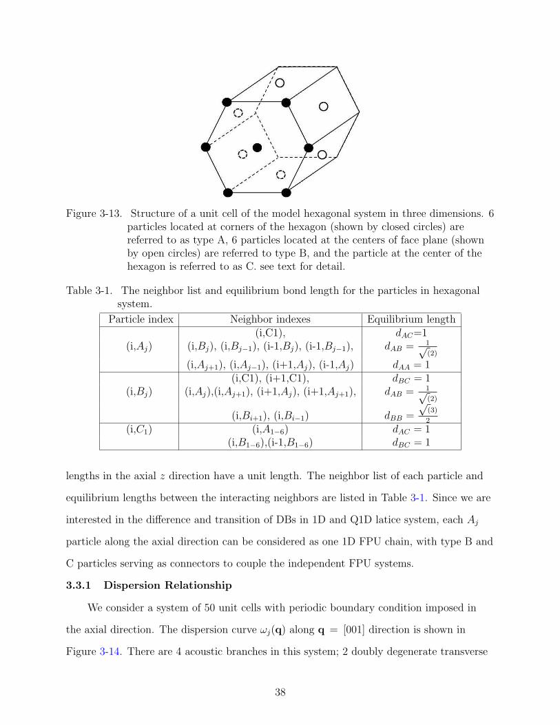
Figure 3-13. Structure of a unit cell of the model hexagonal system in three dimensions. 6particles located at corners of the hexagon (shown by closed circles) arereferred to as type A, 6 particles located at the centers of face plane (shownby open circles) are referred to type B, and the particle at the center of thehexagon is referred to as C. see text for detail.
Table 3-1. The neighbor list and equilibrium bond length for the particles in hexagonalsystem.
Particle index Neighbor indexes Equilibrium length(i,C1), dAC=1
(i,Aj) (i,Bj), (i,Bj−1), (i-1,Bj), (i-1,Bj−1), dAB = 1√(2)
lengths in the axial z direction have a unit length. The neighbor list of each particle and
equilibrium lengths between the interacting neighbors are listed in Table 3-1. Since we are
interested in the difference and transition of DBs in 1D and Q1D latice system, each Aj
particle along the axial direction can be considered as one 1D FPU chain, with type B and
C particles serving as connectors to couple the independent FPU systems.
3.3.1 Dispersion Relationship
We consider a system of 50 unit cells with periodic boundary condition imposed in
the axial direction. The dispersion curve ωj(q) along q = [001] direction is shown in
Figure 3-14. There are 4 acoustic branches in this system; 2 doubly degenerate transverse
38
0 1 2 30
1
2
3
Wave vector k
Fre
quen
cy
Figure 3-14. The dispersion curves for three-dimensional hexagonal tube system.
acoustic (TA) modes, which have x and y vibrations perpendicular to the axial (z)
direction. Single highest energy acoustic mode is the longitudinal acoustic (LA) mode in
the axial direction. The fourth acoustic mode is related to a rotation around the axis,
which is called a twisting mode (TW).
39
1 50−0.03
0
0.03
Dis
plac
emen
t
Unit Cell
XYZ
A
−1 0 1−1
0
1
Re(µ)
Im(µ
)
B
Figure 3-15. A) One of the linear phonon modes of the hexagonal system with(k,β)coupling/FPU = (1, 0). B) Stability analysis for this solution.
3.3.2 Steady State Solutions
Similar to the two dimensional systems considered in section 3.2.3, we first obtain
the steady state solutions for linear system (α = β = 0), which is obtained via
Newton’s method with phonon mode solutions as initial guess. The solution and its
Floquet multipliers are plotted in Figure 3-15. Compared to the linear solutions in two
dimensional system, the linear solutions are linearly stable due to the presence of higher
constraint in both axial and radial directions. More interesting, the gap in this unit circle
is only observed in this system and it exists for three of the linear vibration modes we
computed. To obtain nonlinear localized solution, we assign the breather solutions with
(k, β)FPU = (1, 2) to the axial direction displacement in each chain. In the calculation,
we gradually increase the values of kcoupling and βcoupling with given increasing ω value.
The structure for initial guess is shown in Figure 3-16. The dependence of amplitude and
frequency on varying kcoupling (βcoupling) while keeping βcoupling (kcoupling) fixed is shown in
Figure 3-17. As it is shown in this plot, increasing kcoupling will decrease the localization
of the solutions and while increasing βcoupling supports localized vibration modes. This
relation can be illustrated in the comparison of the configurations of nonlinear modes
where (k, β)coupling = (0.1, 0.1), (1,0.1) and (1,1) are plotted in Figure 3-20 A), B) and C)
respectively. It is clear that increasing kcoupling weakens the localization of the solutions;
while solution with larger values of βcoupling supports highly localized structures.
40
20 27 34
−0.35
0.35
Unit CellZ
Dis
plac
emen
t
Figure 3-16. Initial guess for the Newton’s method for hexagonal system. This vibrationmode corresponds to breather solution in 1D FPU system with k = 1 andβ = 2.
0.5 1
0.2
0.25
0.3
Am
plitu
de
0.5 1
2.51
2.61
2.71
Fre
quen
cy
βcoupling
A
0.5 10.3
0.35
0.4
0.45
Am
plitu
de
0.5 12.62
2.68
Fre
quen
cy
kcoupling
B
Figure 3-17. Dependence of amplitude and frequency of a steady-state mode on thestrength of coupling between chains in hexagonal system. A) βcoupling isvaried; kcoupling = 1 is fixed B) kcoupling is varied with βcoupling = 1 fixed.
Detailed structure of one of the converged nonlinear solution corresponding to
(k, β)coupling = (1, 1) is shown in Figure 3-18 along with its stability analysis. It shows
that increasing coupling strength reduces the magnitude of unstable Floquet multipliers.
The stability analysis in plot D indicates that this mode is still linearly unstable solution.
Since we remove the cause of instability from system configuration, here we examine the
instability from RWA approximation. Therefore, we seek the solution without using RWA
approximation and compare these two solutions. In other words, in the system without
applying RWA approximations, we solve the system of equations for xn,1 and xn,3 using
41
20 27 34
−1.e−2
1.e−2
Unit Cell
X D
ispl
acem
ent
A
B
C
A
20 27 34
−1.e−2
1.e−2
Unit Cell
Y
B
20 27 34
−0.3
0.3
Unit Cell
Z
C
−1 0 1
−1
0
1
Re(µ)
Im(µ
)
D
Figure 3-18. One of the nonlinear solutions with (k, β)coupling = (1, 1). Plots A), B) andC) show the displacement in x, y and z direction respectively. D Stabilityanalysis for this solution.
the Newton’s method. The initial guess are the solutions under RWA approximation. The
results from both approaches are plotted in Figure 3-19. The comparison of xn,1 vector for
both solutions is shown in Figure 3-19 A) and the higher frequency term, xn,3 is plotted in
Figure 3-19 B).
Firstly, the magnitude of xn,3 is 2 orders smaller than xn,1, and quantitative similarity
for xn,1 in two solutions indicate the appropriate assumption of ignoring higher frequency
terms in this system. In order to ensure the validity of RWA approximation in higher
dimensional systems, we compare their Floquet multipliers in Figure 3-21 A), where
the multipliers for the solution using and not using RWA approximation are shown
by diamonds and pluses, respectively. The comparison of two pairs of eigenvectors
corresponding to close Floquet multipliers are shown in Figure 3-21 and Figure 3-22. It is
clear that the first pair correspond to the same perturbation vector. For the second pair,
42
20 27 34−0.4
0.4
Unit Cell
Z D
ispl
acem
ent
3w
w
A
20 27 34−6.e−3
6.e−3
Unit Cell
Z D
ispl
acem
ent
B
Figure 3-19. The comparison of solutions with and without RWA. A) shows the cos(ωt)vector B) the cos(3ωt) vector
20 27 34
−0.35
0.35
Unit Cell
Z D
ispl
acem
ent
A
B
C
A
20 27 34
−0.35
0.35
Unit Cell
Z D
ispl
acem
ent
B
20 27 34
−0.35
0.35
Unit Cell
Z D
ispl
acem
ent
C
Figure 3-20. Comparison of nonlinear modes of hexagonal system for three differentstrengths of coupling between chains of atoms: A) (k, β)coupling = (0.1, 0.1);B) (k, β)coupling = (1.0, 0.1); C) (k, β)coupling = (1.0, 1.0); The linear andnonlinear forces weaken and strengthen localization of the solution structure,respectively.
even it has qualitative different value but these two vectors have the same period, which
implies the RWA approximation should still be valid in this system.
3.3.3 Conclusions
We have investigated the existence and stability of nonlinear vibration modes in
Q1D lattice model systems with various dimensionality. The DBs in 1D FPU system
are obtained from continuation of the nonlinearity strength in the interaction potential.
The unstable eigenvectors correspond to exciting the steady state breathers into moving
breathers. We also observed the complex stability pattern while introducing the cubic
43
−1 0 1
−1
0
1
Re(µ)
Im(µ
)
A
25 50 75 100
−0.15
0
0.15
B
Figure 3-21. A) Stability analysis for the solutions with (without) RWA approximationby diamond (cross) markers. B) Comparison of the z-direction eigenvectorsfor two close eigenvalues shown as open triangle and circular markers.Equivalent vectors are observed.
−1 0 1
−1
0
1
Re(µ)
Im(µ
)
A
25 50 75 100
−0.04
0
0.04
B
Figure 3-22. A) Stability analysis for the solutions with (without) RWA approximationby diamond (cross) markers. B) Comparison of the z-direction eigenvectorsfor two close eigenvalues shown as open triangle and circular markers.Different perturbation vectors are observed.
potential function. Due to the high frequency value for breather solutions, they have
extremely long life time in NEMD simulations. In higher dimensions model system,
we showed the existence of localized nonlinear vibration modes in both two and three-
dimensional systems. However, there are no linearly stable nonlinear vibration modes
under the particular interaction parameters that we explored in this chapter. We
44
also present the cause for instability due to interaction potential and as well as system
configuration.
45
CHAPTER 4NONLINEAR LATTICE VIBRATIONAL MODES IN CARBON NANOTUBES
Investigations of thermal conductivity of carbon nanotubes, along with various
other properties of these materials, is a subject of active research. Review of the recent
literature reveals that the values of thermal conductivity obtained in the experimental
studies [21, 22] significantly differ from the results of the molecular dynamics simulations
[23–26, 59]. Moreover, different MD simulations techniques lead to different results.
These studies have used two complementary MD techniques: the non-equilibrium and
equilibrium molecular dynamics simulations (referred to as NEMD and EMD respectively).
The NEMD simulations consist of imposing the temperature gradient along the
nanotube axis by coupling the opposing ends of the nanotube to the thermal baths
at different temperatures. This coupling is typically implemented by using one of the
thermostat techniques [60]. The thermal flux between the nanotube and the thermal bath
is computed and the thermal conductivity is obtained from the Fourier’s law (1–1). The
EMD simulations are based on simulations in an equilibrium ensemble and the thermal
conductivity is computed from the fluctuations of the thermal flux in the system using the
Green-Kubo formula of the linear response theory [4]. Hence, both the NEMD and EMD
methods are derived in the framework of the linear response theory, which assumes that
the relationship between the perturbation (i.e. temperature gradient) and the response
(i.e. the heat flux) is linear. The discrepancy between the results of these simulations
suggests that the assumption of linear response is not valid in the case of the carbon
nanotubes and nonlinear effects play a significant role.
Recent analyses [61, 62] have shown that nonlinear lattice vibrations in carbon
nanotubes may lead to formation of strongly nonlinear localized waves (solitons). These
studies have considered lattice vibrations in the continuum limit and approximated
nanotubes by a one-dimensional chain of atoms, thus neglecting the details of the lattice
vibration in the directions normal to the nanotube axis. Under these assumptions, it
46
has been shown that the vibrations of the carbon nanotubes can be approximated by
the Korteweg-de Vries (KdV) equation. It is well known that the soliton solutions of the
KdV equation possess constant speed and their interaction can be modeled by elastic
collisions. Therefore, the energy transfer by these solitons is purely ballistic as opposed
to the diffusive heat transfer assumed by the Fourier’s law Eq. 1–1. We note that this
treatment is somewhat approximate since in real nanotubes the heat transport will be
due to a mix of the ballistic and diffusive effects. In particular, it is expected that the
nonlinear localized structures will differ from the idealized KdV solitons in that the
collisions between them will be non-elastic and thus will lead to the transfer of energy
between the localized vibration modes.
In this chapter, we present the investigation of the nonlinear localized vibration
modes in carbon nanotubes, while accounting for the molecular details of the nanotube
structure into account.
4.1 System Configuration
The structure of a nanotube is obtained by rolling a graphite sheet (see Figure 4-1)
into a cylinder [63]. The position r of each carbon atom on the unrolled graphite sheet can
be described by two basis vectors a1 and a2,
r = l1a1 + l2a2, (4–1)
defined in Figure 4-1, where l1, l2 are integers. The structure of a carbon nanotube is
specified by the vector (−→OA) which corresponds to a section of the nanotube perpendicular
to the nanotube axis (−−→OB). A carbon nanotube is constructed by rolling the graphite
sheet so that points O and A coincide. The vectors−→OA and
−−→OB define the chiral vector,
Ch and translation vector T in axial direction. This chiral vector can be expressed in
terms of the basis vectors a1 and a2,
Ch = na1 + ma2 ≡ (n,m) (4–2)
47
The values of n and m determine the chirality of the nanotube, which in particular affects
the electronic conductivity and other properties of the nanotube. A carbon nanotube is
metallic if the value (n −m) is divisible by three and is semiconducting otherwise. Since
we focus on the contribution of lattice vibration modes on thermal transport, we consider
a zigzag semiconductor (5,0) CNT (see Figure 4-1 B).
A
B
Figure 4-1. A) Preparation of a computational model for a nanotube by rolling thegraphite sheet in a direction specified by the chiral vector Ch(n, m) [63]; B)nanotube with chiral vector Ch(5, 0).
We have implemented the Brenner parametrization [64] of the Tersoff potential,
referred to as VB, to describe the interaction between carbon atoms [65, 66]. This
potential has been used in the past for thermal conductivity calculations, as well as
for investigations of other properties of CNTs [67–69]. The explicit potential function is
48
Table 4-1. Parameters for Brenner-Tersoff interaction potential between carbon atoms.
Parameter Value
Re 1.39 AD 6.0 eVβ 2.1 A−1
S 1.22δ 0.5
R1 1.7 AR2 2.0 Aa0 0.00020813c0 330d0 3.5
presented in Eq. 4–3 and the parameters are listed in Table. 4-1.
Vi =∑
j( 6=i)[f(rij)A(rij)−Bijf(rij)C(rij)],
f(rij) = 12[1 + cos(π
rij−R1
R2−R1)], R1 ≤ rij ≤ R2,
A(rij) = DS−1
exp(−β√
2S(rij −Re)),
C(rij) = DSS−1
exp(−β√
2/S(rij −Re)),
Bij = [1 +∑
k(6=i,j) G(θijk)f(rik)]−δ,
G(θijk) = a0[1 +c20d20− c20
d20+(1+cosθijk)2
].
(4–3)
In order to ensure that the equilibrium positions of the carbon atoms are consistent
with the implemented potential. We use the conjugate gradients method [70] to adjust
the equilibrium atom coordinates so that the total potential energy of the nanotube
is minimized. Since our calculation require gradually increase the nonlinearity in the
potential function, we approximate the Brenner potential by a Taylor series up to the
fourth power,
un = −∑m
∂2V
∂un∂um
um − ε
[1
2
∑
m,l
∂3V
∂un∂um∂ul
umul +1
6
∑
m,l,k
∂4V
∂un∂um∂ul∂uk
umuluk
],
(4–4)
so that we can gradually increase the nonlinearity ε for atomic interaction. The 2nd, 3rd,
and 4th derivatives of the potential energy function VB that are necessary in the analysis
are computed numerically by the central finite difference scheme.
49
In order to estimate the importance of the nonlinearity of interatomic interactions in
the nanotube, we compute the ratio |Fn|/|Fl| of the averaged magnitudes of the linear and
the nonlinear components of the force acting on the carbon atoms,
|Fl| =
∣∣∣∣∣∑m
∂2V
∂un∂um
um
∣∣∣∣∣ (4–5)
|Fn| =
∣∣∣∣∣1
2
∑
m,l
∂3V
∂un∂um∂ul
umul +1
6
∑
m,l,k
∂4V
∂un∂um∂ul∂uk
umuluk
∣∣∣∣∣ . (4–6)
Here, the atomic displacements {un} are taken to be those of the normal phonon modes
with the amplitude assigned, according to the Boltzmann distribution at the temperature
T = 300 K, i.e,
1
2m
∑n
un2 =
1
2kBT. (4–7)
. The force ratios |Fn|/|Fl| for the nanotube phonon modes within a single unit cell system
are shown in Figure 4-2. For comparison, we show similar ratios for the FPU system
discussed in chapter 3. It is clear that the magnitudes of nonlinearity of these two systems
are comparable and therefore we expect that the carbon nanotubes possess the nonlinear
vibration modes qualitatively different from the normal phonon modes.
0.7 0.8 0.9 1
0.08
0.12
0.16
ω/ωmax
|Fn|/|
Fl|
FPU
(5,0) Nanotube
Figure 4-2. Ratio of the magnitude of the nonlinear |Fn| and linear |Fl| forces acting onthe equilibrium linear phonon modes of the (5,0) nanotube (♦) and the FPUlattice at α = β = 1 (•). Here, ωmax is the maximum phonon frequency of thesystem.
50
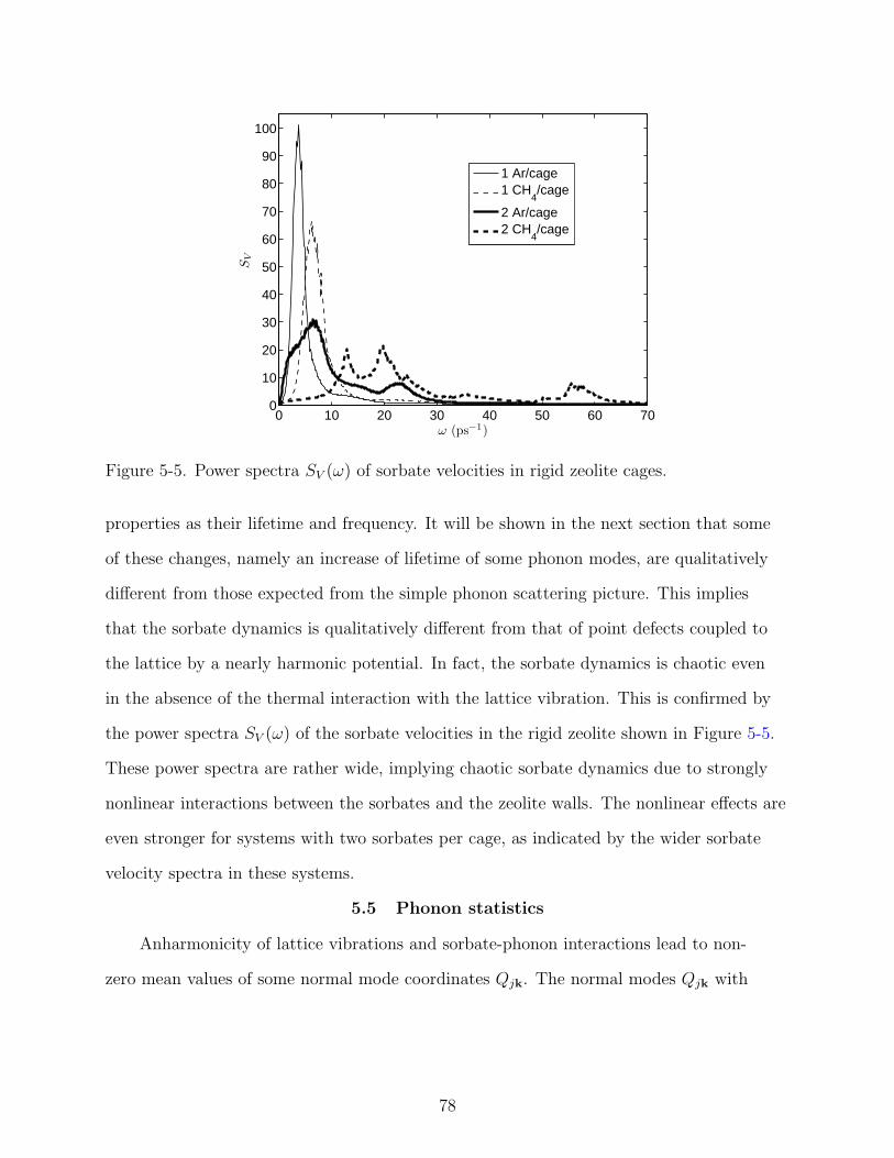
4.2 Non-Equilibrium MD Simulation
In order to assess the propagating structures in the carbon nanotubes during
heat transfer, we perform NEMD simulation for a 100 unit-cell (43.2 nm) nanotube
with chirality (5,0) and impose periodic boundary condition along z-axis. We set up
a temperature gradient by imposing two thermostats of 300K and 280K on the 50th
and the first unit cell of the nanotube via Berendsen algorithm. We use velocity Verlet
time integration scheme with time-step dt = 0.1fs. After the system has reached
equilibrium, the temperature gradient is obtained by a linear fit of the average nanotube
cell temperatures which gives T ′(z) = 0.45 Knm
. The developed temperature profile is
shown in Figure 4-3 A); the evolution of local energy distribution is shown in the Figure 4-
3 B). The local energy is the sum of the kinetic and potential energy of an individual
unit cell. This reveals that a part of energy is transferred by localized packets and that
ballistic transport mechanism does play an important role in carbon nanotube systems. To
determine the corresponding heat carriers for this phenomena, we solve the equations of
motion to obtain the steady state solutions in carbon nanotubes.
4.3 Steady States Solutions in CNTs
As described in chapter 2, we obtain steady-state solutions using Newton’s method.
Since VB potential is closely approximated by VT potential at ε = 1, initial guesses for the
Brenner modes are taken to be the Taylor modes with ε = 1 and the latter are obtained
by perturbing the linear normal modes (ε = 0) with analytical approximations from
perturbation theory , and using these approximations as initial guess for potential VT ,
followed by a continuation of the solution by increasing ε until it reaches 1.
The normal modes and dispersion curve are obtained from the following eigenvalue
problem [71]:
ω2un =∑m
∂2V
∂un∂um
um ≡ −F(un) (4–8)
where ω is the vibration frequency. We computed the phonon dispersion curves for the
(5,5) carbon nanotubes, and observed that these are in good agreement with the results of
51
10 20 30 40280
290
300
Position [nm]
Tem
pera
ture
[K]
A
B
Figure 4-3. NEMD simulations of a segment of a (5,0) CNT. The system contains 100unit cells and contains a heat source at the center (in the 50-th unit cell) anda heat sink in the first cell: A) Temperature profile of the system ; B) Thelocal energy transport in a steady-state system
molecular dynamics simulations reported in Ref. [26]. The dispersion curve for the (5,0)
carbon nanotubes is presented in Figure 4-4.
52
2 4 6
100
200
300
Wave vector k [1/nm]
Fre
quen
cy [
1012
Hz
]
Figure 4-4. Phonon dispersion curves of the (5,0) carbon nanotube under Brenner-Tersoffpotential.
The unknowns for equations of motion are the atomic displacement, which are
expressed using the Fourier series as in Eq. 2–15. The frequency ω is a fixed and given
parameter during the iterations of the Newton’s method. We impose periodic boundary
conditions in the axial direction and also apply RWA approximation, i.e, the coefficients
xn,j with j ≥ 2 are neglected. The numerical solution of Eq. 2–2 requires a function
which, given the Fourier series expansions for the atom displacements ul(t), computes
the Fourier series expansions for the force Fn(u) acting on the atoms. For sufficiently
simple potentials Fn(u) can be obtained analytically by direct substitution of u into
an expansion for F. For more complex potentials, such as the Brenner potential, we
use the following procedure summarized in Figure 4-5. Given Fourier coefficients x for
atomic displacements u, we perform inverse Fourier transform to obtain values of u(t)
at evenly spaced times tj within one period of oscillations. Then we compute forces
fk(tj) = fk(u(tj)) acting on each atom and perform Fourier transform on the force vectors
at times of t1, . . . , tj. Practically, we solve the equations of motion set up for zeroth
and first Fourier mode coefficients. The nonlinear solutions x(ε) are obtained through
continuation by Newton’s method from normal modes solutions, which represent ε = 0
solutions. The Jacobian matrix in Eq. 2–17 is obtained from central finite difference
scheme. We will refer to nonlinear modes of CNTs obtained with potentials VT and VB as
Taylor and Brenner modes (solutions), respectively.
53
Figure 4-5. The summary of the numerical procedure to obtain Fourier series expansionfor a complex potential. Here, fft and ifft denote fast Fourier transform andinverse fast Fourier transform.
Application of Newton’s method to potential VB is extremely time consuming, mainly
due to the necessity of using a finite-difference scheme to compute Jacobian matrix J .
On the other hand, J for VT potential can be obtained analytically, which allows us to
obtain the solutions relatively fast even in large systems. Therefore, nonlinear solutions
for periods exceeding 2 are obtained for VT potential only. Moreover, for systems with
period exceeding 2, we neglect the cubic terms and approximate VT potential as a sum
of quadratic and quartic terms. The solution corresponding to such a potential does not
include a static displacement term (see Eq. 3–2), which reduces the number of unknowns.
This simplifications allows us to obtain the steady state solutions with periods up to 24
unit cells.
4.4 Results
In this section, we present the solutions for the Taylor and the Brenner potentials for
different number of unit cells. In these calculations, ω is a given parameter and the results
for different values of ω illustrate the role of this parameter. First we describe the results
for a single unit cell nanotube, which consists of two carbon rings. The result in Figure 4-6
is obtained using the phonon mode with frequency ω0 = 3.125 × 10¹⁴ Hz as the starting
54
point. The steady-state vibration mode corresponding to the nonlinear Brenner-Tersoff
potential was obtained using a series of solutions of Eq. 4–4 with gradually increasing
magnitude of nonlinearity ε. The step for ε is chosen to be ∆ε = 0.02. The initial
condition for the solution of the nonlinear system at ε = 0.02 was obtained from the linear
mode using the regular perturbation analysis. We obtained ∆ω(ε = 0.02) = 1.25× 10¹¹ Hz
from this perturbation analysis. During the process of the continuation by parameter ε,
ω was changed at every step by the same value, ∆ω = 1.25 × 10¹¹ Hz up to β = 0.68
and then is kept as constant to β = 1. We note that although for the first step the value
of ω was dictated by the perturbation method, the changes in ω in the consecutive steps
were somewhat arbitrary with the goal to obtain a solution with frequency sufficiently
different from that of phonon modes. Once the continuation reached the value of ε = 1,
we used the Newton’s method again to obtain the vibration mode corresponding to the
complete Brenner-Tersoff potential. The nonlinear mode obtained by this method is
shown in Figure 4-6 and is compared with the corresponding linear phonon mode in the
same figure. The displacements in the x and y directions are very similar for atoms of
the two different rings of the nanotube unit cell (both for linear and nonlinear modes),
and thus, we show these displacements for only one of the rings. These results indicate
that the system described by the complete non-linear carbon nanotube potential possesses
vibration modes qualitatively different from those of the linearized systems. In addition
to the large difference in the dynamic displacement of the modes, the nonlinear modes
exhibit large static displacement (see Figure 4-6 B,E) that is absent in the linear modes.
The corresponding mode energy along the continuation by parameter ε is also presented
in Figure 4-7. The left hand side and right hand side y axis represents mode energy and
the frequency respectively, x axis is the value of nonlinearity ε. Even ω value in this
calculation is given arbitrarily, from the initial drop of mode energy for solution with
ε = 0.02 and the constant mode energy while ω is kept constant for ε > 0.68, which implies
the dependence of mode energy on ω.
55
0 0.2
−0.2
0
0.2
Z(nm)
Y(n
m)
[x20]
A
0 0.2
−0.2
0
0.2
Z(nm)
Y(n
m)
[x20]
B
0 0.2
−0.2
0
0.2
Z(nm)
Y(n
m)
[x20]
C
−0.3 −0.2 −0.1 0 0.1 0.2 0.3
−0.2
−0.1
0
0.1
0.2
X (nm)
Y (
nm)
[x20]
D
−0.3 −0.2 −0.1 0 0.1 0.2 0.3
−0.2
−0.1
0
0.1
0.2
X (nm)
Y (
nm)
[x11]
E
−0.3 −0.2 −0.1 0 0.1 0.2 0.3
−0.2
−0.1
0
0.1
0.2
X (nm)
Y (
nm)
[x100]
F
Figure 4-6. Comparison between a linear phonon mode of the (5,0) carbon nanotube andthe nonlinear mode obtained from this mode by the continuation method. Thefirst row of plots [ A), B), C)] shows the displacement of atoms in the zdirection. For clarity, the atoms belonging to the same ring are plotted on thesame line. The second row of plots [ D), E), F)] shows the atom displacementin the x and y directions for one of the nanotube rings. The second ringexhibits similar displacements and hence is not shown. The first column ofplots [ A), D)] shows the linear solution; the second [ B), E)] and the third[ C), F)] columns show respectively the static and the dynamic displacementsof the nonlinear mode. The displacements are shown by arrows which forclarity are magnified by a factor of 20 [all plots except F)] or by a factor of100 [plot F)].
In the two unit cells system, we use ∆ω obtained from degenerate perturbation
for the first step in the continuation curve. During the process of the continuation by
parameter ε, ω is changed only at the first step. The nonlinear mode configuration shown
in Figure 4-8 is obtained using the phonon mode with frequency ω0 = 1.2 × 10⁹ Hz as
the starting point with mode energy corresponding to 350K and ∆ω(ε = 0.02) = −3.1 ×10⁸ Hz. The value of frequency is kept constant until ε reaches 1. In addition, to explore
the energy threshold of initial mode energy for exciting the localized nonlinear vibration
56
0 0.2 0.4 0.6 0.8 10
200
400
Mod
e E
nerg
y [K
J / M
ol]
β0 0.2 0.4 0.6 0.8 1
3.1
3.15
3.2
ω [1
014 H
z]
β
Figure 4-7. Dependence of the mode energy and frequency of the Taylor solutions on ε forsolutions shown in Figure 4-6. The mode energy is shown by diamonds. Thevalue of frequency ω is shown by pluses.
modes as we observed in section 3.2.3 in Q1D model system, we start with the normal
modes with thermal energy corresponding to 200K, 250K and 350K. Below we show
the displacement for the first carbon ring and only compare the dynamical displacement
between nonlinear and linear solutions for the three temperatures. The results for both
Taylor and Brenner solutions and the corresponding mode energy continuation curves
are shown in Figure 4-8. Plots A and D are the displacement for linear system; B and E
are the Taylor solutions for three different initial thermal energy; C and F are Brenner
solutions. This nonlinear vibration modes have configuration similar to the phonon mode
where we started the calculation. The results starting with different temperatures lead
to solutions with similar configuration and Brenner solution is very similar to Taylor
solutions, which justifies our numerical process. The mode energy for these three solution
branches along the continuation by parameter ε are presented in Figure 4-9. Because ωnl
is close to ω0 we obtain the vibration modes with configuration qualitatively similar to the
phonon modes.
For system with simplified potential, we obtain nonlinear vibration modes for 4, 8,
16 and 24 unit cells. In this potential function, we are able to reach nonlinear vibration
57
−0.2 0
−0.2
0
0.2
Phonon; ω=82.4532
[x80]
X (nm)
Y (
nm)
[x80][x80]
A
−0.2 0 0.2
−0.2
0
0.2
ε=1
[x300][x300][x300]
X (nm)
Y (
nm)
B
0 0.2
−0.2
0
0.2
[x80]
Z (nm)
Y (
nm)
[x80][x80]
(D)
C
0 0.2
−0.2
0
0.2
[x80]
Z (nm)
Y (
nm)
[x80][x80]
(D)(D)
D
0 0.2
−0.2
0
0.2
[x300][x300][x300]
Z (nm)
Y (
nm)
E
0 0.2
−0.2
0
0.2
[x300][x300][x300]
Z (nm)
Y (
nm)
F
Figure 4-8. The solutions of (5,0) CNT in two unit cells system starting with theamplitude corresponding to three different temperature. The first row of plots[ A), B), C)] shows the displacement of atoms x and y directions for one ofthe nanotube rings. to the same ring are plotted on the same line. The secondrow of plots [ D), E), F)] shows the atom displacement in the z direction. Forclarity, the atoms belonging The first column of plots [ A), D)] shows thelinear solution; the second [ B), E)] and the third [ C), F)] columns showrespectively the Taylor and Brenner solutions. The displacements are shownby solid lines which for clarity are magnified by a factor shown in the leftcorner in each subfigures.
modes for ε = 1 and ∆ω = 8.6 × 10¹¹ Hz in one step of Newton’s method calculation.
An example of the nonlinear vibration modes with longest length, 24 unit cells is shown
in Figure 4-10, in which the solution is obtained using the phonon mode with frequency
ω0 = 1.58 × 10¹⁴ Hz. Since it is a long system, we present this nonlinear vibration mode
by plotting the dynamical displacement for the 7th atom in each unit cell. Plots A), B)
and C) are the atomic displacement for the nonlinear vibration mode along x, y and z
directions, respectively; and plots D), E) and F) are the dynamical displacement for
linear phonon mode along x, y and z directions, respectively. The nonlinear solution has
58
0 0.2 0.4 0.6 0.8 10
2
4
ε
Mod
e E
nerg
y [ K
J/M
ol ]
0 0.2 0.4 0.6 0.8 182.4526
82.4528
82.453
82.4532
0 0.2 0.4 0.6 0.8 182.453
82.4531
82.4532
0 0.2 0.4 0.6 0.8 182.4528
82.453
82.4532
Fre
quen
cy [
1012
Hz
]
ε
200K250K350K
Figure 4-9. Dependence of the mode energy and frequency of the Taylor solutions startingwith three initial thermal energy on ε for solutions shown in figure 4-8. Themode energy is shown by diamonds. The value of frequency ω is shown bypluses.
the qualitatively similar configuration compared to the initial linear phonon mode. We
observe that in this case the solution is qualitatively different from the initial phonon
mode. In order to summarize the nonlinear solutions for this potential function, we mark
the converged solutions on the dispersion curve in Figure 4-11. Plot A shows the solution
frequency, open (closed) marker represent the solutions with different (same) wave number
(periodicity) from the initial phonon modes. In order to quantify the difference between
nonlinear modes and phonon modes, we normalize the nonlinear solutions and compute
the norm of the difference between these two solutions, the results are plotted in plot B.
It is noted that large differences occurs for solutions for which the wave number equals π2a
,
where a is the length of one unit cell in z direction.
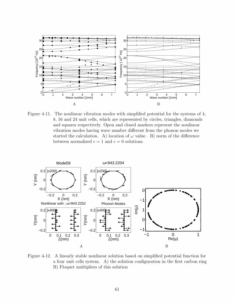
We also perform Floquet analysis for the nonlinear solution in the 4 unit-cell system.
We obtain both linearly stable and unstable vibration modes. The configuration and their
Floquet multipliers are shown in Figure 4-12 and Figure 4-13, respectively. To investigate
the cause for the instability, we plot the eigenvector corresponding to the open circle in
Figure 4-13B in Figure 4-14. We still need to analyze this eigenvector to fully understand
the effect of this unstable perturbation on the nonlinear vibration mode.
59
1 24−0.02
0
0.02
X
Unit Cell
A
1 24−0.04
0
0.04
X
Unit Cell
B
1 24−0.02
0
0.02
Y
Unit Cell
C
1 24−0.04
0
0.04
Y
Unit Cell
D
1 24−0.04
0
0.04
Z
Unit Cell
E
1 24
−0.06
0
0.06
Z
Unit Cell
F
Figure 4-10. The comparison the displacement for the 7th atom in each unit cell for ε = 1nonlinear mode and starting phonon mode in a 24 unit cells system with thesimplified potential under RWA approximation. The first row of plots [ A),B), C)] shows the displacement of atoms for solution. The second row ofplots [ D), E), F)] shows the atom displacement for the starting phononmode. The first, second and third column of plots shows the displacement inx, y and z direction. displacement for the first, fourth and 7th atom in eachunit cell.
4.4.1 Conclusions
We have investigated the thermal transport mechanism in a semiconductor carbon
nanotube. In non-equilibrium MD simulations, localized packets are observed, and this
indicates the important of ballistic transport mechanism in carbon nanotubes. We have
explored the nonlinear vibration modes in carbon nanotubes under Brenner-Tersoff
potential, as well as with simplified force coefficients. Nonlinear vibration modes with
qualitatively different configuration compared to linear phonon modes are obtained.
Among the solutions obtained, there are some stable nonlinear vibration modes. Even
though the structures are not localized, the roles of these nonlinear modes, including
their group velocity and phonon mean free path need further investigation in order to
describe the dynamics of vibration modes in carbon nanotubes using Boltzmann transport
equation.
60
0 1 2 3 4 5 6 70
5
10
15
20
25
30
Wave number [1/nm]
Fre
quen
cy [1
013 H
z]
A
0 1 2 3 4 5 6 70
5
10
15
20
25
30
Wave number [1/nm]
Fre
quen
cy [
1013
Hz]
B
Figure 4-11. The nonlinear vibration modes with simplified potential for the systems of 4,8, 16 and 24 unit cells, which are represented by circles, triangles, diamondsand squares respectively. Open and closed markers represent the nonlinearvibration modes having wave number different from the phonon modes westarted the calculation. A) location of ω value. B) norm of the differencebetween normalized ε = 1 and ε = 0 solutions.
−0.2 0 0.2
−0.2
0
0.2
X (nm)
Y (
nm)
Mode59
[x200]
0 0.1 0.2 0.3−0.2
0
0.2
Z(nm)
Y(n
m)
[x400]
Nonlinear soln ; ω=943.2252
−0.2 0 0.2
−0.2
0
0.2
X (nm)
Y (
nm)
ω=943.2204
[x200]
0 0.1 0.2 0.3−0.2
0
0.2
Z(nm)
Y(n
m)
[x400]
Phonon Modes
A
−1 0 1−1
0
1
−1
0
Re(µ)
Im(µ
)
B
Figure 4-12. A linearly stable nonlinear solution based on simplified potential function fora four unit cells system. A) the solution configuration in the first carbon ringB) Floquet multipliers of this solution
61
−0.2 0 0.2
−0.2
0
0.2
X (nm)
Y (
nm)
Mode171
[x100]
0 0.1 0.2 0.3−0.2
0
0.2
Z(nm)
Y(n
m)
[x100]
Nonlinear soln ; ω=323.2077
−0.2 0 0.2
−0.2
0
0.2
X (nm)
Y (
nm)
ω=323.1938
[x100]
0 0.1 0.2 0.3−0.2
0
0.2
Z(nm)
Y(n
m)
[x100]
Phonon Modes
A
−1 0 1−1
0
1
−1
0
Re(µ)
Im(µ
)
B
Figure 4-13. The nonlinear solution based on simplified potential function for a four unitcells system. Figure A) shows the atomic displacement and its Floquetmultipliers are shown in plot B)
−0.2 0 0.2
−0.2
0
0.2
X (nm)
Y (
nm)
[x1]
A
0 0.1 0.2 0.3
−0.2
0
0.2
Z(nm)
Y(n
m)
[x950]
B
Figure 4-14. The eigenvector corresponding the Floquet multiplier shown as the opencircle in Figure 4-13B.
62
CHAPTER 5EFFECTS OF SORBATE MOLECULES ON THERMAL TRANSPORT IN ZEOLITES
In this and the following chapters we present the investigation of thermal transport
in nanoporous materials including the molecular dynamics simulations for encapsulated
sodalite zeolites and the model development for the sorbate molecule in a 1D model is
reported in chapter 6.
Zeolites are microporous alumino-silicate crystals with pore sizes comparable to
molecular dimensions. They are widely used as molecular sieves, sorbents, catalysts,
and ion exchangers. In addition, several possible applications of zeolites combining
adsorption of guest molecules with temperature control are emerging. Examples include
solar adsorption heat pump [72] and adsorption chillers for microelectronic devices [73].
A wide variety of available zeolite structures provides a large range of flexibility in
fine-tuning their thermal properties to a specific task. Zeolite thermal conductivity can
also be altered by introducing point defects into the crystal lattice, e.g., by substitution
of some of the silicon atoms by aluminum [74]. The point defects provide additional
scattering centers for phonons thus reducing the crystal thermal conductivity [75].
Moreover, the nanoporous structure of zeolites provides an additional opportunity to
control the zeolite thermal properties through introduction of off-framework guest species
(sorbates or cations) into the crystal. In fact, it is well known that strong interaction
between zeolite lattice vibrations and guest molecules significantly affect transport
properties of the guest molecules (see e.g. [76–78]) as well as the dynamics of oscillation
of sorbate molecules at their adsorption sites [79]. Evidence is accumulating that presence
of guest molecules within zeolites also affects the dynamics of zeolite lattice vibrations
leading to changes in thermal properties of zeolites [29, 80].
Similar host-guest interactions play a significant role in thermal conductivity of
other nanoporous materials of technological importance. For example, skutterudites are
promising candidates for development of efficient thermoelectric materials, i.e. materials
63
with high ratio of electrical and thermal conductivities. It has been shown [27, 28] that
addition of ions to voids in skutterudites leads to an order of magnitude decrease of their
thermal conductivity thus increasing the thermoelectric figure of merit.
Available data suggest complex dependence of the thermal conductivity on the
nature of a guest molecule and a host crystal. As discussed above, addition of ions to
skutterudites reduces their thermal conductivity. Similarly, encapsulation of an atom in
a Ge clathrate leads to an order of magnitude reduction in thermal conductivity [81]. In
addition, molecular dynamics (MD) simulations [29] show a drastic reduction of thermal
conductivity of zeolite LTA-SiO2 in the presence of heavy cations. These results seem to
suggest that “rattling” of the guest species inside a crystal leads to scattering of phonons
thus reducing their mean free path and leading to the decrease of thermal conductivity.
However, other observations contradict this picture. For example, MD simulations
of xenon in zeolite LTA-SiO2 indicate an increase of the zeolite thermal conductivity
due to the guest-host interactions [29]. In addition, experiments of Greenstein et al.
[80] show that the conductivity of zeolite MFI is substantially higher when an organic
template cation tetrapropylammonium (TPA) is present in it, as compared to a sample
with removed templates.
Therefore, the phonon-guest interactions may be qualitatively different from
the phonon scattering by point defects fixed in the lattice due to strongly nonlinear
oscillations of guest molecules inside the crystal pores. Interactions of guest molecules
with host lattice vibrations have been extensively modeled in recent years [78, 79, 82–84].
Typically, the goal of these studies is to understand effects of the lattice vibration on the
sorbate dynamics inside crystals and the lattice vibrations are frequently modeled as a
thermal bath. In the current work, we are aiming at understanding the reverse process,
i.e. effects of the sorbate “rattling” on the crystal lattice vibrations. In this chapter
we present results of our investigations of effects of sorbate molecules on dynamics of
individual phonons. It is expected that understanding of sorbate-phonon interactions
64
will lead to a better understanding of the sorbate effects on thermal conductivity of
nanoporous materials. We consider a relatively simple system, namely a sodalite zeolite
with small molecules (argon, xenon, or methane) trapped inside its cages. Forces between
these sorbates and zeolite lattice atoms are short-ranged and, when the sorbate size is
sufficiently small, the interaction between the sorbate and the phonons takes place only
during collisions between the sorbate and the zeolite wall. Therefore, the current model
allows us to focus on effects of the sorbate “rattling” on the phonon dynamics and our
observations are not obscured by other possible contributions of guest molecules to the
lattice dynamics, such as long-range electrostatic interactions between adsorbed charged
species and lattice ions.
5.1 Model Details
The crystal structure of silica sodalite Si12O24 is shown in Figure 5-1. This zeolite
possesses a cubic symmetry and its lattice parameter is 8.83 A, see [85]. A sodalite
unit cell consists of a cage shaped like a truncated cuboctahedron bounded by six 4-
ring windows (i.e. windows formed by four oxygen and four silicon atoms) and eight
6-ring windows. Diameter of the 4-ring windows is very small and these windows are
impermeable by the sorbates considered in our simulations. In addition, transport rates of
argon and larger molecules (methane and xenon) through the 6-ring windows are orders
of magnitude slower than the phonon-phonon and phonon-sorbate interactions [77] and a
sorbate remains inside a cage on the time-scale of interest.
Silica sodalite is usually synthesized by growing the crystal around organic template
molecules which become encapsulated in the sodalite cages after the synthesis is complete
[85, 86]. In the current work, we neglect the presence of encapsulated templates and
perform MD simulations of either bare silica sodalite containing only Si and O atoms in its
lattice structure or silica sodalite with encapsulated argon, methane, or xenon molecules.
The equilibrium lattice configuration and the potential model for zeolite lattice
vibrations used in this study are the same as those used by Kopelevich and Chang [77]
65
Figure 5-1. A block of 2× 2× 2 sodalite unit cells containing nine sodalite cages. Siliconand oxygen atoms are shown as larger and smaller spheres, respectively. InMD simulations of sorbate-lattice systems, the sorbates are located in eightcorner cages of this block.
in a study of sorbate transport through 6-ring windows. Zeolite lattice vibrations are
modeled by a truncated version of an anharmonic potential energy field proposed by
Nicholas et al. [87],
V (u) =∑O−Si
Vr(rO−Si) +
∑O−Si−O
Vα(αO−Si−O) +∑
Si−O−Si
[Vβ(βSi−O−Si) + VUB(rSi−Si)
], (5–1)
where
Vr(r) =1
2Kr(r − rO−Si
0 )2 (5–2)
is the potential energy of stretching of the O-Si bond r,
Vα =1
2Kα(α− α0)
2 (5–3)
66
is the potential energy of bending of the O-Si-O bond angle α,
Vβ =1
2
[K
(1)β (β − β0)
2 −K(2)β (β − β0)
3 + K(3)β (β − β0)
4]
(5–4)
is the potential energy of bending of the Si-O-Si bond angle β, and
VUB(r) =1
2KUB(r − rSi−Si
0 )2 (5–5)
is the Urey-Bradley term which represents lengthening of the Si-O bond as the Si-O-Si
angle becomes smaller. In Eq. 5–5, r denotes distance between two silicon atoms of a
Si-O-Si angle.
The potential model Eq. 5–1 neglects smaller contributions included in the original
model [87] such as torsion energy of the dihedral Si-O-Si-O angle, nonbonded Lennard-
Jones interaction, and electrostatic interaction between zeolite atoms due to the partial
charges of Si and O atoms. In principle, long-range electrostatic interactions may have
a significant effect on the lattice dynamics. However, it has been shown in [87] that
electrostatic interactions have little effect on the structure or dynamics of the silica
sodalite lattice due to high symmetry of this crystal and charge neutrality of each SiO2
group. Moreover, since the sorbates considered in the current work are electrically neutral,
electrostatic interactions with the partial charges of the lattice atoms are expected to have
negligible effects on the sorbate dynamics. In fact, this truncated model has been shown
to yields good agreement between computed and experimental values of transport rates
of inert gases in sodalite [77]. Since this transport process involves large deformations of
6-ring windows, it is expected that, despite the introduced approximations, the model
Eq. 5–1 provides an accurate description of anharmonic lattice dynamics.
The values of the force constants K as well as the values of the equilibrium distances
(rO−Si0 and rSi−Si
0 ) and equilibrium bond angles α0 and β0 are summarized in Table 5-
1. The force constants and the equilibrium bond angles were taken from the paper
of Nicholas et al. [87]. The equilibrium distances rSi−Si0 and rO−Si were obtained from
67
Table 5-1. Parameters for the lattice potential energy model Eq. 5–1.
Si-O Kr = 2500.1 kJ mol−1 A−2 rO−Si0 = 1.58 A
O-Si-O Kα = 578.1 kJ mol−1 rad−2 α0 = 109.5◦
Si-O-Si K(1)β = 45.4 kJ mol−1 rad−2 β0 = 149.5◦
K(2)β = 95.1 kJ mol−1 rad−3
K(3)β = 55.5 kJ mol−1 rad−4
Si-Si KUB = 228.5 kJ mol−1 A−2 rSi−Si0 = 3.1219 A
Table 5-2. Lennard-Jones parameters for sorbate-sorbate and sorbate-lattice interactions.
yields frequencies ωjk of the normal mode vibrations.
The normal mode coordinates can now be defined as follows [71]
Qj(k) = (L1L2L3)−1/2
∑
l
N∑κ=1
3∑α=1
m1/2κ uα(lκ)e∗α(κ; jk)e−ik·r(l). (5–10)
In the case of a harmonic and sorbate-free lattice, the normal modes are independent
of each other and the Hamiltonian of each mode is
Hjk =1
2|Qjk|2 +
1
2
(ωh
jk
)2 |Qjk|2. (5–11)
Here and in the remainder of the chapter, we use superscript h to distinguish frequency of
a normal mode in a harmonic lattice from that in an anharmonic lattice.
The sodalite unit cell contains N = 36 atoms. Therefore, there are 108 normal
modes corresponding to each wavevector k. Since in the current work we consider a
2 × 2 × 2 block of unit cells and sodalite possesses a cubic symmetry, there are only
four independent wavevectors, k = [000], [100], [110], and [111], in our MD system. For
reference, the dispersion relationships ωhj (k) for sodalite for wavevectors k pointing in
directions [100], [110], and [111] are shown in Figure 5-2. Normal modes accessible by the
MD simulations correspond to the smallest and the largest values of |k| in each of these
three plots.
In general, encapsulation of a sorbate inside a zeolite cage may affect the linearized
lattice dynamics and lead to changes in the eigenvectors of the dynamical matrix, which
would require one to use different normal modes in the analysis of zeolite lattice vibration
in the presence of sorbates. However, this effect is significant only in the case of strong
interaction between phonons and a sorbate located at an equilibrium adsorption site.
This situation would occur if the sorbate fits tightly within a zeolite cage or if there are
71
0 0.05 0.1 0.15 0.2 0.25 0.3 0.350
20
40
60
80
100
120
140
160
180
200
220
|k|, (A−1)
ωh
(ps−
1)
A
0 0.1 0.2 0.3 0.4 0.50
20
40
60
80
100
120
140
160
180
200
220
|k|, (A−1)
ωh
(ps−
1)
B
0 0.1 0.2 0.3 0.4 0.5 0.60
20
40
60
80
100
120
140
160
180
200
220
|k|, (A−1)
ωh
(ps−
1)
C
Figure 5-2. Dispersion relationships for sodalite in directions (A) k = [100], (B) k = [110],and (C) k = [111].
long-range electrostatic interactions between the sorbate and the zeolite lattice. It has
been shown in [84] that coupling between the phonon modes and small electrically neutral
sorbates, such as those considered in the current work, is negligible when the sorbates are
located at adsorption sites inside sodalite cages. For these systems, the sorbate-phonon
coupling becomes significant only when the sorbate approaches the zeolite wall. Therefore,
the presence of the sorbates does not affect the dynamical matrix of the crystal.
The nonlinear effects of the sorbates, such as the change in phonon lifetime and the
nonlinear corrections to the phonon frequency are analyzed in the next two sections.
The insensitivity of the harmonic approximation to the lattice dynamics to the sorbates
considered in the current work allows us to use the normal modes of the sorbate-free
72
zeolite to analyze the lattice dynamics in the presence of the sorbates. In the remainder
of the chapter, we use harmonic phonon frequencies ωhjk to parameterize various plots of
properties of individual modes. This allows us to consistently identify a phonon mode even
if its frequency is changed upon addition of various sorbates.
5.4 Nonlinear phonon and sorbate dynamics
Nonlinear phonon dynamics is usually modeled by the Boltzmann transport equation
BTE [75]
vjk · ∇T∂njk
∂T=
(∂njk
∂t
)
collision
, (5–12)
where T is the temperature and vjk and njk are the group velocity and the occupation
number of the phonon mode jk. The occupation number njk is proportional to the
harmonic potential energy of the mode jk, see, e.g., [93]. Phonon-phonon interactions due
to lattice anharmonicity, defects, and other factors are modeled by the collision integral
in the right-hand-side of Eq. 5–12. Calculation of the collision integral in exact form is
very challenging and it is usually approximated by various models, such as the single mode
relaxation time (SMRT) approximation,
(∂njk
∂t
)
collision
=neq
jk − njk
τjk
. (5–13)
Here, neqjk is the equilibrium phonon distribution and τjk is the relaxation time of the
phonon mode jk, which is assumed to coincide with the phonon lifetime. The relaxation
time can be estimated from MD simulations by computing relaxation times of the
occupation number [93] or the harmonic energy (5–11) of the normal mode [94].
The analysis of the phonon dynamics based on BTE approach has several drawbacks.
The relaxation time approximation may not be adequate to model phonon dynamics
in complex materials. Although SMRT approximation (5–13) can be extended to
account for multiple relaxation times due to different phonon scattering mechanisms,
these extensions require the phonon autocorrelation function to be a sum of multiple
exponentials. However, as will be shown below, some of the sodalite phonon modes do not
73
satisfy this requirement. In this case, a straightforward extension of the relaxation time
model does not seem to be possible. In addition, the relaxation time approximation may
not be appropriate to account for phonon-sorbate interactions.
In order to attain more flexibility in modeling phonon dynamics, we choose an
alternative model based on Langevin equation [12],
Qjk + γjkQjk = (ωajk)
2 (Qjk − 〈Qjk〉) + Γjk(t). (5–14)
Here, 〈Qjk〉 is the mean value of the normal mode coordinate Qjk, which may differ from
zero due to anharmonicity of the system, ωajk is the anharmonic frequency, γjk is the
friction coefficient, and Γjk(t) is the random force with zero mean which is related to the
friction coefficient by the fluctuation-dissipation theorem
〈Γjk(t)Γjk(t + τ) = 2kBTγjkδ(τ). (5–15)
We assume that the deterministic force in this Langevin model is still harmonic and the
anharmonicity of the oscillations can be adequately captured by shifts in the phonon
frequency and average normal mode coordinates, as well as friction and stochastic forces.
The autocorrelation function of normal mode Qjk satisfying equation (5–14) is [95]
Cjk(τ) = 〈δQjk(t)δQ∗jk(t + τ)〉 = e−τ/τjk cos ωjkτ. (5–16)
Here,
δQjk = Qjk − 〈Qjk〉 (5–17)
is the deviation of the phonon mode from its average,
τjk = −2/γjk (5–18)
is the phonon lifetime, and
ωjk =√
(ωajk)
2 − 1/τ 2jk. (5–19)
74
is the apparent phonon frequency. Eq. 5–16 demonstrates that, similarly, to BTE with
SMRT approximation, the Langevin model (5–14) predicts an exponential decay of
the normal mode autocorrelation function. However, the Langevin equation provides
more flexibility and allows one to perform relatively simple adjustments of the model to
fit observed phonon dynamics. This can be done by including an explicit anharmonic
term into the equation or modifying statistics of the random force. For example, non-
exponential behavior of the autocorrelation function can be modeled by a non-Markovian
random force [96].
Examples of phonon autocorrelation functions obtained from our MD simulations
of sorbate-free sodalite are shown in Figure 5-3. Most of these functions, such as that
shown in Figure 5-3a, are in good agreement with Eq. 5–16. However, some modes
exhibit significant deviations from the predictions of this Markovian Langevin equation.
Autocorrelation functions of all these non-Markovian modes are qualitatively similar
to one of the autocorrelation functions shown in Figure 5-3b-d. These modes possess
secondary (slow) oscillations which are qualitatively similar to oscillations of the
autocorrelation function of the energy of an entire sodalite cage observed by McGaughey
and Kaviany [97]. These secondary oscillations were interpreted as corresponding to
localization of energy in sodalite cages. Our analysis of individual phonon modes shows
that only a fraction of optical phonons modes possesses this secondary time-scale.
In the current work we assume that the Markovian Langevin equation (5–14) provides
an adequate model for the phonon dynamics and leave development of its extensions
to acount for secondary oscillations to future studies. Therefore, the lifetimes and
the frequencies of all modes are obtained by applying Eq. 5–16 to analysis of their
autocorrelation function
In particular, Eq. 5–16 implies that the power spectrum Sjk(ω) of the phonon mode
jk attains its maximum at ω = ωjk. Therefore, we define the apparent frequency of
vibration, ωjk, as the location of the maximum of Sjk(ω) for all modes, including those
75
0 2 4 6−1
−0.5
0
0.5
1
τ (ps)
Cjk
A j = 7
0 2 4 6−1
−0.5
0
0.5
1
τ (ps)
Cjk
B j = 23
0 2 4 6−1
−0.5
0
0.5
1
τ (ps)
Cjk
C j = 64
0 20 40−1
−0.5
0
0.5
1
τ (ps)C
jk
D j = 104
Figure 5-3. Examples of autocorrelation functions Cjk(τ) of phonons in a sorbate-freesodalite crystal. The normal mode numbers j are shown in the correspondingplots; the wavevector is k = [000] in all four examples. In plots A) and B),envelopes ±Ejk(τ) of the autocorrelation functions are shown by dashed lines.
exhibiting significant deviations from Eq. 5–16. Typical examples of power spectra of the
normal modes are shown in Figure 5-4. We observe that for most modes, even those not
satisfying the Langevin model (5–14), the maximum of Sjk corresponds to the highest
frequency of oscillations which we associate with the apparent phonon frequency. In a
few cases, such as that shown in Figure 5-4c, the maximum of Sjk corresponds to slower
secondary oscillations. In these cases, the apparent phonon frequency was defined as the
frequency of a local maximum of Sjk(ω) with the largest value of ω.
In order to estimate the lifetime of a phonon mode, we define an envelope Ejk(t) of
its autocorrelation function Cjk(t) as a line connecting local maxima of Cjk(t), as shown
by dashed lines in Figure 5-3a,b. The function Ejk is then fitted to an exponential. In the
cases of non-exponential decay of Ejk, the phonon lifetime is obtained by fitting its initial
(quickly decaying) segment to an exponential.
76
0 50 100 1500
50
100
150
200
ω (ps−1 )
Sjk
A j = 7
0 50 100 1500
50
100
150
200
ω (ps−1 )
Sjk
B j = 23
0 50 100 1500
50
100
ω (ps−1 )
Sjk
C j = 64
0 100 200 3000
500
1000
ω (ps−1 )
Sjk
D j = 104
Figure 5-4. Power spectra Sjk(ω) corresponding to the phonon autocorrelation functionsshown in Figure 5-3. The normal mode numbers j are shown in thecorresponding plots and the wavevector is k = [000] in all four examples.
Once the apparent phonon frequency ωjk and the lifetime τjk are obtained, the
anharmonic phonon frequency ωajk is computed from Eq. 5–19. This equation is correct
only for phonon normal modes that satisfy the Markovian Langevin equation (5–14).
However, the differnce between ωjk and ωajk is negligible if ωjk >> 1/τjk. As will be shown
in section 5.5, phonon lifetimes range from 0.4 to 30 ps. Therefore, the correction of the
apparent frequency (5–19) is significant only for phonons with very small frequencies.
Our results indicate that dynamics of the low-frequency modes are in good agreement
with the predictions of Eq. 5–14, see e.g. Figure 5-3a. The correction of the apparent
frequency is accurate for these modes. On the other hand, this correction is negligible for
the high-frequency modes which do not satisfy the Markovian model (5–14).
Autocorrelation functions Cjk of a phonon mode jk in a sorbate-free sodalite and a
sodalite containing sorbates are qualitatively similar for the same values of j and k. This
provides an additional confirmation that small neutral sorbates do no alter the phonon
eigenmodes (see discussion at the end of section 5.3). The sorbates affect such phonon
77
0 10 20 30 40 50 60 700
10
20
30
40
50
60
70
80
90
100
ω (ps−1)
SV
1 Ar/cage1 CH
4/cage
2 Ar/cage2 CH
4/cage
Figure 5-5. Power spectra SV (ω) of sorbate velocities in rigid zeolite cages.
properties as their lifetime and frequency. It will be shown in the next section that some
of these changes, namely an increase of lifetime of some phonon modes, are qualitatively
different from those expected from the simple phonon scattering picture. This implies
that the sorbate dynamics is qualitatively different from that of point defects coupled to
the lattice by a nearly harmonic potential. In fact, the sorbate dynamics is chaotic even
in the absence of the thermal interaction with the lattice vibration. This is confirmed by
the power spectra SV (ω) of the sorbate velocities in the rigid zeolite shown in Figure 5-5.
These power spectra are rather wide, implying chaotic sorbate dynamics due to strongly
nonlinear interactions between the sorbates and the zeolite walls. The nonlinear effects are
even stronger for systems with two sorbates per cage, as indicated by the wider sorbate
velocity spectra in these systems.
5.5 Phonon statistics
Anharmonicity of lattice vibrations and sorbate-phonon interactions lead to non-
zero mean values of some normal mode coordinates Qjk. The normal modes Qjk with
78
Table 5-3. Normalized averages of phonon amplitudes, ∆Qjk =< Qjk > /σjk. Only modeswith sufficiently large average deviations from zero, ∆Qjk ≥ 0.04, are shown.Normal modes are listed in the order of descending ∆Qjk. Harmonic phononfrequencies ωh
jk corresponding to the listed modes are also shown.
sufficiently large relative deviation of their mean from zero,
∆Qjk =〈Qjk〉σjk
≥ 0.04, (5–20)
are listed in Table 5-3. In Eq. 5–20, σjk denotes the standard deviation of the normal
mode fluctuations.
In the sorbate-free lattice, modes Qjk with j = 7 and j = 63 and k = [000] deviate
from zero by 4 and 3 standard deviations, respectively. All other modes have much smaller
deviations, ∆Qjk < 0.02. Addition of one sorbate per cage essentially does not change
the values of ∆Qjk. However, addition of two sorbates per cage leads to a substantial
shift of average values of several additional modes, implying that the equilibrium lattice
configuration slightly changes due to the presence of the sorbates. This change is larger
in the case of 2 CH4/cage. Addition of 2 CH4/cage shifts averages of several normal
modes away from zero as well as further increases ∆Qjk of the modes j = 7 and j = 63
(k = [000]) that were already shifted in the sorbate-free lattice. Nevertheless, even the
strongest sorbate effects on the mean normal coordinates seen in the case of 2 CH4/cage
are significantly weaker than effects of introduction of anharmonicity to a harmonic
sodalite lattice.
79
0 50 100 150 200 2500
5
10
15
20
25
30
ωhjk (ps−1)
τjk
(ps)
Figure 5-6. Phonon lifetimes τjk in sorbate-free sodalite lattice.
It is interesting to note that all substantial shifts of 〈Qjk〉 take place for optical lattice
modes with k = [000]. The largest relative displacement of an acoustic mode is rather
small (∆Qjk = 0.048) and is observed for mode j = 1,k = [110] when 2 CH4/cage are
added.
Phonon lifetimes τjk in sorbate-free anharmonic lattice range from 0.4 to 30 ps, as
shown in Figure 5-6. The modes with intermediate frequencies, 70 ps−1 ≤ ωhjk ≤ 150 ps−1,
possess short lifetimes. The phonons with high frequencies, ωhjk > 150 ps−1, correspond
mostly to fast vibrations of individual bonds. Interactions between these modes and other
modes in the system are weak leading to large phonon lifetimes for the high-frequency
modes. Some modes with low frequencies, ωhjk < 70 ps−1, also possess long lifetimes.
However, most of the low-frequency modes possess relatively short lifetimes indicating that
they are strongly coupled with other modes in the system.
For comparison, analysis of McGaughey and Kaviany [97] based on a decomposition
of the heat current autocorrelation function predicts decay time for heat transfer
associated with long-range acoustic modes in sodalite to be 1.67 ps. In addition,
80
Greenstein et al. [80] have estimated phonon relaxation time in MFI zeolite to be 9.2 ps
by fitting a theoretical expression to experimental thermal conductivity data. This
estimate is based on an assumption that the relaxation time is the same for all phonon
modes. Both of these estimations are within the range of the phonon lifetimes observed in
the current work.
Relative changes of phonon lifetimes,
δτjk =τ sjk − τa
jk
τajk
, (5–21)
upon encapsulation of sorbates into the zeolite cages are shown in Figure 5-7. In Eq. 5–
21 and elsewhere in this chapter superscript s refers to a property related to a zeolite
with encapsulated sorbates. The distributions of δτjk shown in Figure 5-7a are almost
identical for all three systems with 1 sorbate/cage. These distributions are symmetric with
respect to δτ = 0, which implies that the phonon-sorbate interactions are equally likely
to decrease as well as increase the phonon lifetime. The increase of the phonon lifetime
contradicts a simple picture of phonon scattering by sorbates and implies that a more
complex sorbate-phonon interaction is in play.
When two sorbates per cage are added to the system, the distribution of δτjk
becomes skewed towards average decrease of the phonon lifetime. This trend is especially
pronounced in the case of a larger sorbate, namely methane. This can be explained,
in part, by a tighter fit of the sorbates within the cages leading to a smaller amplitude
of the sorbate oscillations, which suggests more similarities between sorbates in these
systems with point defects. However, as Figure 5-5 indicates, the sorbate dynamics in the
2 sorbate/cage systems is more chaotic than in the 1 sorbate/cage systems. Therefore,
the analogy between the 2 sorbates/cage systems and crystals with point defects is not
complete. Indeed, Figure 5-7 shows that some of the phonon modes in the 2 sorbates/cage
systems undergo a significant (on the order of 100%) increase of their lifetime and hence
the scattering model is still not applicable to this case.
81
In order to assess which of the modes undergo increase or decrease of their lifetime,
in Figure 5-7b we plot δτjk for every phonon mode. For clarity, only two extreme cases
are shown: 1 Ar/cage and 2 CH4/cage. For 1 Ar/cage, the changes of phonon lifetimes are
evenly distributed among different frequencies. In the 2 CH4/cage system, the modes lying
in the small and large frequency regions experience, on average, larger change of their
lifetimes than the modes with intermediate frequencies.
Effects of anharmonicity on the phonon frequency in a sorbate-free sodalite crystal are
summarized in Figure 5-8 which shows relative differences,
δωjk =ωa
jk − ωhjk
ωhjk
, (5–22)
between the anharmonic and harmonic phonon frequencies. With few exceptions,
anharmonicity leads to an increase of the phonon frequency. This increase is especially
large for low frequency modes.
Addition of sorbates to zeolite cages typically leads to a further frequency increase, as
can be seen from the relative differences
δωsjk =
ωsjk − ωa
jk
ωajk
(5–23)
between phonon frequencies in sodalite with encapsulated sorbates (ωsjk) and in the
sorbate-free sodalite (ωajk), see Figure 5-9. The frequency changes δωs
jk are substantially
larger when more than one sorbate per cage is introduced. Similarly to δωjk, δωsjk tends
to increase with the decrease of the phonon frequency. However, the changes of phonon
frequencies due to addition of sorbates are smaller than the changes due to introduction of
anharmonicity to a sorbate-free harmonic lattice.
Up to this point, we have investigated effects of anharmonicity and sorbate-phonon
interactions on individual phonon modes. To complete the picture, we now consider
correlations between different phonon modes. It is expected that this information will
be helpful in developing a more precise form of the Langevin model (5–14) for phonon
82
−1 −0.5 0 0.5 10
0.5
1
1.5
2
2.5
3
δτjk
P(δ
τjk)
1 Ar/cage
1 CH4/cage
1 Xe/cage
2 Ar/cage
2 CH4/cage
A
0 50 100 150 200−1
−0.5
0
0.5
1
1.5
ωhjk (ps−1)
δτjk
1 Ar/cage
2 CH4/cage
B
Figure 5-7. Effects of sorbates on phonon lifetimes. A) Distributions P (δτjk) of therelative differences δτjk between the phonon lifetimes τ s
jk in sodalite withencapsulated sorbates and the phonon lifetimes τa
jk in a sorbate-free sodalite.B) Relative changes δτjk of lifetimes of individual modes jk for the cases of1 Ar/cage and 2 CH4/cage.
83
0 50 100 150 200 250−0.1
0
0.1
0.2
0.3
0.4
0.5
0.6
0.7
0.8
ωhjk (ps−1)
δω
jk
Figure 5-8. Relative differences δωjk between the anharmonic (ωajk) and harmonic (ωh
jk)frequencies in a sorbate-free sodalite crystal.
0 20 40 60 80 100−0.25
−0.2
−0.15
−0.1
−0.05
0
0.05
0.1
0.15
0.2
ωhjk (ps−1)
δω
s jk
1 Ar/cage1 CH
4/cage
1 Xe/cage2 Ar/cage2 CH
4/cage
Figure 5-9. Relative differences δωsjk between phonon frequencies in sodalite with
encapsulated sorbates (ωsjk) and in the sorbate-free sodalite (ωa
jk). For clarity,only δωs
jk with magnitudes greater than 10−2 are shown.
84
0 50 100 150 2000
50
100
150
200
ωhjk (ps−1)
ωh j′k
′(p
s−1)
0.08
0.16
0.24
0.31
0.39
0.47
Figure 5-10. Magnitudes of correlation coefficients ρ(jk, j′k′) between phonon modes jkand j′k′ in a sorbate-free sodalite crystal. Darker symbols correspond tostronger correlations. For clarity, correlation coefficients for jk = j′k′ are notshown and only correlations of magnitude greater than 0.1 are plotted.
dynamics since it will allow us to assess which phonons make dominant contributions to
stochastic forces acting on each of the phonon modes. The magnitudes of the correlation
coefficients
ρ(jk, j′k′) =
∣∣∣∣〈δQjkδQ
∗j′k′〉
σjkσj′k′
∣∣∣∣ (5–24)
between modes jk and j′k′ in a sorbate-free lattice are shown in Figure 5-10. For clarity,
only correlations of magnitude exceeding 0.1 are plotted. Most correlation coefficients
between individual phonons are rather weak. Correlations between low- and mid-
frequency modes constitute a notable exceptions: some correlations of low-frequency
modes with modes of frequency ωhjk ≈ 100 ps−1 have correlation coefficient as large as
0.5. These observations are consistent with the measured phonon lifetimes, see Figure 5-6.
Specifically, phonon-phonon correlations involving the high-frequency modes are very
weak, which is manifested in long lifetimes of these modes. The modes with intermediate
frequencies, 70 ps−1 ≤ ωhjk ≤ 150 ps−1, are strongly correlated with some of the low
frequency modes, which leads to small lifetime of these modes.
85
0 50 100 150 2000
50
100
150
200
ωhjk (ps−1)
ωh j′k
′(p
s−1)
2 Ar/cage
2 CH4/cage
0.08
0.16
0.24
0.31
0.39
0.47
Figure 5-11. Effect of sorbates on phonon-phonon correlations. Only those pairs (jk, j′k′)are shown for which addition of sorbates creates a correlation with coefficientgreater than 0.1 or changes the magnitude of an existing correlation by morethan 0.1. Magnitudes of the changed correlation coefficients are indicated bycolor.
Effect of the sorbate presence on the phonon-phonon correlations is shown in
Figure 5-11. Addition of a single sorbate per cage leads to relatively small changes in
phonon-phonon correlations, with no phonon pairs with correlation coefficient greater than
0.1 being affected. Addition of 2 Ar/cage creates one new phonon-phonon correlation with
magnitude slightly larger than 0.1. In contrast, addition of 2 CH4/cage creates several
strong correlations and magnifies some correlations which were present in the sorbate-free
lattice. The largest changes of the correlation coefficients upon addition of 2 CH4/cage are
between the low-frequency acoustic modes with wavevector k = [110] and other phonons.
The change of the correlation coefficient in these cases is ∆ρ ≈0.27.
5.5.1 Conclusions
We have investigated phonon dynamics in sodalite for five different sorbate-zeolite
systems: 1 Ar/cage, 1 CH4/cage, 1 Xe/cage, 2 Ar/cage, and 2 CH4/cage, as well as
86
a sorbate-free zeolite. We have observed that the Markovian Lanvegin equation (5–
14) provides an adequate model for dynamics of most of the phonon modes. However,
dynamics of some phonon modes does not agree with predictions of Eq. 5–14. These
modes exhibit secondary oscillations (see Figure 5-3b-d) which are most likely related to
the total energy fluctuations inside a single sodalite cage [97].
Encapsulation of sorbates in zeolite cages does not lead to qualitative changes of
phonon dynamics, as can be concluded from phonon autocorrelation functions. However,
depending on the type and number of sorbates inside sodalite cage, some or all of the
following aspects of phonon dynamics are changed: (i) the mean values of the normal
mode coordinates, (ii) phonon lifetimes, (iii) phonon frequencies, and (iv) phonon-phonon
correlations. The largest changes of phonon dynamics are observed upon encapsulation of
two methane molecules per sodalite cage.
The strongest effect of all considered sorbates on lattice dynamics is a significant
change of the phonon lifetimes. From the scattering picture of phonon-sorbate interactions
it is expected that these interactions will decrease phonon lifetimes. However, we observe
that encapsulation of sorbates leads to an increase of lifetimes of a large fraction of
phonons. Therefore, development of a more detailed model is necessary to understand the
complex nonlinear sorbate-phonon interactions.
87
CHAPTER 6MODEL DEVELOPMENT FOR SORBATE MOLECULES IN 1D SYSTEM
In this chapter, we present results of our efforts to develop a mathematical model
for the “rattling” effect of sorbate molecules on the lattice vibration of a host matrix.
Existing models for phonon scattering cannot be directly applied because they are limited
to prediction of phonon interaction with static impurities or defects [98]. To investigate
the influence of sorbates on lattice system and to develop a heat transfer model for
nanoporous materials, we consider a simple 1D system. First, we investigate dependence of
thermal conductivity of this system on sorbate properties using full scale non-equilibrium
MD simulations. To get insight into the sorbate-lattice dynamics, we investigate phonon-
sorbate dynamics in a harmonic lattice, which allows us to focus on the role of the
sorbate-lattice interactions in the energy exchange between phonon modes. In conclusion,
we discuss possible approaches to development of a theoretical model.
6.1 Thermal Conductivity from NEMD Simulations
We consider FPU system (see section 3.1) consisting of N = 1024 particles with force
constants k = 10, α = −50, and β = 180. The sorbate is located between lattice sites 256
and 257 and interacts with the lattice atoms through Lennard-Jones (LJ) potential:
VLJ = 4ε
[(σ
r
)12
−(σ
r
)6]
, (6–1)
where r is the distance between the sorbate and a lattice atom. Periodic boundary
conditions are imposed in the system. Hot and cold regions with temperatures Th = 1.2
and Tc = 0.8 each containing 100 particles are set up at the edge (atoms 1, . . . , 100) and
at the center (atoms 512, . . . , 612) of the chain using the Nose-Hoover thermostat (see
section 2.2.2). We use velocity Verlet algorithm with time step ∆t = 5 × 10⁻⁴ time unit.
The simulation is carried out for 225000 time units. After the system reaches a steady
state, we compute the heat flux
J =1
2
∑
m6=n
vnfnm, (6–2)
88
1 500 1000
0.8
1
1.2
Position
Tem
pera
ture
A
1 500 1000−1.5
0
1.5
Position
Hea
t Flu
x
B
Figure 6-1. A) Established temperature profile in non-equilibrium MD simulations. Thesorbate is located between lattice sites and sorbate-lattice interactions aremodeled by LJ potential. B) Established heat flux in non-equilibrium MDsimulations.
where vn is the velocity of the n-th atom and fnm is the force with which the m-th atom
is acting on the n-th atom. The thermal conductivity κ is then calculated using Fourier’s
law, Eq. 1–1. We perform a series of NEMD simulations with sorbates of different mass
Ms and Lennard-Jones parameter ε of sorbate-lattice interaction. In all these simulations,
the effective LJ diameter is σ = 0.23. Examples of established temperature and heat
flux profiles are shown in Figure 6-1. Comparison between thermal conductivities of a
sorbate-free lattice and lattice containing various sorbate molecules is shown in Figure 6-2.
Even in this simple system, we observe a complex pattern of dependence of κ on the
sorbate-lattice interaction parameters. The presence of the sorbate may either increase
or decrease the thermal conductivity. In addition, sufficiently large temperature gradient
leads to development of a discontinuity in the temperature profile across the unit cell
containing the sorbate, as shown in Figure 6-3. This phenomenon is similar to Kapitza
thermal boundary resistance at an interface between two dissimilar materials [99]. In the
latter case, a temperature discontinuity is developed to maintain continuity of the heat
flux through the interface.
89
0 0.5 1 1.5 2 2.55.2
5.4
5.6
5.8
6
6.2
6.4
6.6
6.8
Ms/ε
The
rmal
Con
duct
ivity
[ κ
]
With Sorbate
pure lattice
Figure 6-2. Comparison of thermal conductivities, κ, obtained from NEMD simulationsfor a system containing 1024 atoms. Temperature gradient in all simulations isdTdx
= 0.001. Solid circles represent the values of κ in the presence of a sorbatemolecule with mass Ms and LJ interaction parameters ε. The solid linecorresponds to the thermal conductivity of lattice with no sorbate molecules.
1 250 500
0.9
1.0
1.1
Particle
Tem
pera
ture
Figure 6-3. Steady state temperature profile in NEMD simulation with imposedtemperature gradient dT
dx= 0.002 The sorbate is located between lattice
particles 128 and 129. A discontinuity in the temperature profile is developedacross the unit cell containing the sorbate.
90
6.2 Sorbate in a Harmonic Lattice
In order to isolate the phonon-phonon energy exchange facilitated by the sorbate from
the energy exchange due to lattice anharmonicity, in the remainder of this chapter we
consider dynamics of a sorbate in a harmonic lattice. The Hamiltonian of the system is
H =∑
q
Hq + Hs + U({Qj}, xs), (6–3)
where
Hq =1
2
(ω2
q |Qq|2 + |Qq|2)
, (6–4)
is the Hamiltonian of a phonon mode Qq with wavenumber q,
Hs =Msv
2s
2+ U0(xs) (6–5)
is the Hamiltonian of a sorbate in a rigid lattice, and U({Qj}, xs) is the potential energy
of interactions between the phonons and the sorbate. In Eq. (6–4), ωq is the frequency of
the phonon with wavenumber q, which is given by the following dispersion relationship,
ωq =
√4k
m
∣∣∣∣sin qa
2
∣∣∣∣ (6–6)
(a is the lattice constant, m is the mass of lattice atoms). In Eq. (6–5), Ms, xs, and vs
are the sorbate mass, position, and velocities, respectively, and U0(xs) is the potential of
interaction between the sorbate and the lattice atoms when the latter are fixed at their
equilibrium positions.
In the absence of the sorbate-lattice coupling, i.e. when U({Qj}, xs) ≡ 0, the system
is integrable; the phonons and the sorbate undergo periodic motion. Introduction of a non-
zero potential U({Qj}, xs) perturbs their periodic trajectories. It is known from the theory
of dynamical systems [100] that a small perturbation of an integrable systems may lead
to a complete destruction of the periodic trajectories. In this case, the system trajectory
becomes chaotic, which facilitates fast energy exchange between the system degrees of
freedom. Such chaotic behavior will take place if the unperturbed system satisfies the
91
resonance condition, i.e. if the ratio of frequencies of some of the unperturbed periodic
trajectories is a rational number.
6.2.1 Scattering of a Phonon Wavepacket
In this section we discuss simulations of scattering of a phonon wavepacket by a
single sorbate located in a harmonic lattice. Similar simulations have been performed in
Ref [101] for scattering of a wavepacket by an interface between two different crystals.
We consider one-dimensional harmonic lattice containing N = 2001 atoms. The
sorbate is located between lattice sites 1000 and 1001. The lattice spring constant is
k = 156 and the sorbate-lattice interactions are modeled by LJ potential, Eq. 6–1. The
mass of sorbate molecule, Ms, ranges from 1 to 6 and ε ranges from 1 to 10, while effective
LJ diameter is held fixed at σ = 0.44.
The sorbate does not move until a collision with a wavepacket. The simulations are
initialized with the sorbate placed at its equilibrium position within a unit cell and its
initial velocity set to zero. Initial lattice configuration consists of a phonon wavepacket
centered at wavenumber q0. This wavepacket is a linear combination of the normal modes
with wave numbers sufficiently close to q0. Therefore, the displacement ul of the l-th
lattice atom is
ul = Aeıq0(xl−x0)e−η2(xl−x0)2 , (6–7)
where A is the amplitude of the wave and
uq = ei(qx−ωqt) (6–8)
is a normal mode corresponding to wavenumber q.
This procedure generates a wavepacket localized in space around x0 with spatial
extent ∼ 1/η. The value of the parameter η is selected so that the range of wave numbers
in the generated wavepacket is sufficiently narrow. This ensures that the wavepacket
maintains its configuration until its collision with the sorbate. The initial velocities of the
92
1000 2000
−0.1
0.1
Position
Dis
plac
emen
tTime=1
A
1000 2000
−0.1
0.1
Position
Dis
plac
emen
t
Time=271
B
1000 2000
−0.1
0.1
Position
Dis
plac
emen
t
Time=500
C
Figure 6-4. Scattering of a wavepacket centered around wavenumber q0 = 0.1π by asorbate with LJ parameters (ε, σ) = (2, 0.44) and mass Ms = 1. Location ofthe unit cell containing the sorbate molecule is shown by the dashed line.
1 2 3 4 5 60
0.2
0.4
0.6
0.8
1
Mass of sorbate
Tra
nmis
sion
Rat
io
q0=0.2π ; ω=7.7155
q0=0.5π ; ω=17.6566
q0=0.8π ; ω=23.7525
Figure 6-5. Transmission ratios for scattering of different wavepackets by sorbatemolecules with different masses. LJ potential parameters are (ε, σ) = (2, 0.44)in all shown simulations.
lattice atoms are obtained as follows. We decompose ul into the normal modes and then,
using the normal mode frequencies, obtain the time derivatives of the atom displacements.
A typical example of the wavepacket scattering is shown in Figure 6-4. As can be
seen, a part of the wavepacket is transmitted through the unit cell containing the sorbate
molecule and part of the wavepacket is reflected. The frequency of the normal modes
contained in these wavepackets remain essentially unchanged.
Transmission ratios (i.e., ratios of the amplitude of the transmitted and the incident
wavepackets) for a series of the scattering simulations are summarized in Figure 6-5. In
93
these simulations, LJ parameters were fixed, σ = 1.0 and ε = 0.44, and the sorbate
mass Ms and wave numbers q0 of the incident wavepackets were varied. Depending on q0,
the transmission ratio may either monotonously increase, monotonously decrease as Ms
is increased. We also observe a sudden drop of the transmission ratio to an almost full
reflection for q0 = 0.5π and Ms = 2. These parameters correspond to a resonance between
the sorbate and the wavepacket.
In order to further study the resonant sorbate-lattice interactions, we perform
two scattering simulations using the same wavepacket with different parameters of the
sorbate molecule. We estimate the sorbate frequency from the linear approximation of LJ
potential,
VLJ ' 1
2kLJ(r − r0)
2, (6–9)
ωs '√
kLJ
Ms
. (6–10)
The wavepacket is centered around normal modes with wavenumber q0 = 0.475π and
ω = 16.9 with fixed effective LJ parameter σ = 0.44. We use two different values of
Ms and ε for the sorbate molecule: (0.5,5) and (1,1). We refer to these two interaction
parameters as system α and β, respectively. From Eq. 6–9, the sorbate frequency is
ωs = 16.8 and 5.36, respectively. Hence the sorbate frequency in system β is closer to the
resonance frequency with the wavepacket.
The initial configuration of the wavepacket is shown in Figure 6-6 A). The system
configurations after the wavepacket pass the sorbate molecule in system α and β are
shown in Figure 6-6 B) and C), respectively. There is a qualitative difference between
scattering results for these two wavepackets. Under resonance condition (system β),
wavepacket changes its shape, which suggests that additional modes are excited due
to interaction with this wavepacket. In order to obtain a better view of the scattering
process, we perform windowed-Fourier transform (WFT) of the lattice configuration.
This transform allows us to obtain local wave numbers of the lattice modes for different
94
1000 2000−0.05
0.05
Particle Position
Dis
plac
emen
t
A
1000 2000−0.05
0.05
Particle Position
Dis
plac
emen
t
B
1000 2000−0.05
0.05
Particle Position
Dis
plac
emen
t
C
D E F
Figure 6-6. Scattering of wavepackets with wave numbers with q = 0.475π with fixedsigma = 0.44 and (Ms,epsilon)=(0.5,5) and (1,1). A) Initial wavepacketconfiguration for both simulations.; B) System configuration after scatteringwith sorbate for (Ms,epsilon)=(0.5,5); C) System configuration afterscattering with sorbate for (Ms,epsilon)=(1,1); D) to F) are WindowedFourier transforms of configurations shown in A) to C); x axis corresponds tolattice sites and y axis corresponds to local wave numbers of latticeoscillations.
locations within the system. The results of WFTs for Figure 6-6 A)- C) are shown in
Figure 6-6 D)- F), respectively. In the system α (plot E), the wavepacket structure and
wavenumber remain the same as in the initial wave packet (plot D). This is expected
as this value of the initial wave vector is sufficiently far from the resonant condition.
On the other hand, in the system β we observe that the symmetric structure of the
wavepacket is destroyed and nearby wave modes are excited during the collision. This
quick redistribution of energy between different modes is characteristic of a resonant
system.
95
0 200 400 6000
10
20
30
Time
Ene
rgy
Ms=0.1, ε=2
Ms=1, ε=0.5
Ms=1, ε=1.5
Figure 6-7. Evolution of mode energy for incident plane wave with wavenumberq = 0.245π interacting with different sorbate molecules. Ms = 1, σ = 0.23 andthree ε values of 0.5, 1.5, 2.
6.2.2 Scattering of a Plane Wave
The wavepacket scattering simulations reveal the dependence of energy transport on
interaction in lattice system. However, due to the short time span of the sorbate-phonon
interactions in these simulations, we cannot obtain information regarding long-term energy
dispersion among the normal modes.
In order to get better insight of the phonon-sorbate interaction dynamics, we perform
scattering simulations of a plane wave. The initial conditions for these simulations are
plane waves consisting of a single normal modes. The lattice spring constant in these
simulations is k = 78. The simulations are performed for time length of 600 time units.
We perform a series of MD simulations with planar wave consisting of single phonon
mode, ωin = 6.6 Hz. We present the analysis of the results including incident mode
energy evolution, sorbate frequency and energy dispersion from three sets of interaction
parameters: σ is fixed to be 0.23 and (Ms, ε) = (0.1, 2), (1, 0.5) and (1, 1.5). These three
systems are referred to as system A, B and C respectively. The incident mode energy
evolution in Figure 6-7 shows that the energy change in both systems A and C are in
the form of periodic oscillation whereas rapid decaying behavior is observed in system
B. Note that in this harmonic system the energy exchange between different normal
96
5 10 150
0.05
0.1
ωs
| Fou
rier
Coe
ffici
ent |
A
5 10 150
0.02
ωs
| Fou
rier
Coe
ffici
ent |
B
5 10 150
0.02
0.04
0.06
ωs
| Fou
rier
Coe
ffici
ent |
C
Figure 6-8. Fourier transform of the sorbate displacement with Ms = 1, σ = 0.23 andε =0.5 A), 1.5 B) and 2.0 C) respectively.
0 5 10 150
0.5
1
1.5
2
ωin
∆ E
Ms=0.1d0, ε=2.d0
Ms=1.d0, ε=0.5d0
Ms=1.d0, ε=1.5d0
Figure 6-9. Dispersion of incident mode energy (q = 0.245π) among other phonon modesunder different values of sorbate mass. Ms = 1, σ = 0.23 and three ε values of0.5, 1.5, 2.
modes only occurs through sorbate-phonon interaction. Thus, rapidly decaying behavior
indicates the sorbate-phonon interaction allows significant dispersion of incident mode
energy among the other normal modes. The condition for occurrence of energy change
between two degrees of freedom is the resonance condition. Hence we present the sorbate
frequency spectrum in Figure 6-8. As expected, we observe a wide frequency spectrum for
system B. Moreover, in order to identify the dispersion of energy among the other phonon
modes, we plot the gained energy of the other phonon modes except the incident mode
in Figure 6-9. In system A, there is almost no energy transfer taking place, implying
weak interaction between sorbate and other phonon modes. This is also verified by the
97
very distinct sorbate frequency spectrum shown in Figure 6-8A. On the other hand, the
excitation of most phonon modes is observed for system B (closed circles). Note that
though in Figure 6-8B the magnitude at high sorbate frequency is not as significant
as that for lower frequency, the higher frequency phonon modes are excited due to the
satisfaction of resonance condition
ω = mωs. (6–11)
We also observe the excitation of modes with 2ωin = 13.30 Hz in the system C.
From these results we conclude that the energy exchange between phonon modes
through rattling of sorbate molecules depends on the frequency spectrum of sorbate
molecule. Sorbate molecule with wide frequency spectrum excites most normal modes
and on the other hand, sorbate molecule with distinct frequency is considered as a small
perturbation to the dynamics of incident phonon mode and hence only excites modes with
close frequencies. In order to understand the dependence of sorbate frequency spectrum
on sorbate-lattice interaction parameters and further quantify the energy exchange, we
present the possible approaches to develop a mathematical model using both dynamical
system approach and multi-scale expansion.
6.2.3 Possible Theoretical Approach: Multi-scale Expansion
In this section we initiate development of an analytical model for the phonon
scattering by sorbate molecules. The first step in this development is to describe the
above scattering process. We consider a simplified linear lattice-sorbate interaction as
in this simple model one can obtain an analytical solution which fully describes this
system. However, our eventual goal is to develop an approach that may be extended to
nonlinear interactions between the lattice and the sorbate. In the absence of the sorbate,
displacement of lattice atoms can be fully described by orthonormal eigenvectors φk(x)
and ±ıωk eigenvalues in a linear system. We also consider the presence of sorbate as
a perturbation to the linear system with new set of eigenvector ψk(x) and eigenvalue
98
±ıνk. Since φk and ψk are complete set of basis vectors, the displacement throughout the
scattering process can be expanded as follows:
f(x, t) =∑
k[Fk(t)eıωkt + Gk(t)e
−ıωkt]φk(x)
=∑
j[Ajeıνjt + Bje
−ıνjt]ψj(x).(6–12)
In addition, these two sets of eigenvectors are connected by constant matrix Γ given by
−→Ψ = Γ
−→Φ . (6–13)
Substituting Eq. 6–13 into Eq. 6–12, we obtain the relation
Fk(t)eıωkt + Gk(t)e
−ıωkt =∑
j
γjk(Ajeıνjt + Bje
−ıνjt) (6–14)
In a weakly perturbed system
νk = ωk + ενk, ε → 0, (6–15)
and thus the time-dependent coefficients, Fk(t) and Gk(t) will be slow-varying function.
Here another slow time variable, τ is introduced;
Fk(t) ≡ Fk(τ)
Gk(t) ≡ Gk(τ),(6–16)
where τ = εt. Under the weak perturbation assumption, Eq. 6–15, the relation between
these two sets of coefficients, Eq. 6–13, becomes
Fk(τ)eıωkt + Gk(τ)e−ıωkt '∑
j
γjk(Ajeıωkteıνjkτ + Bje
−ıωkte−ıνjkτ ) (6–17)
Comparing both sides of Eq. 6–17,
Fk(τ) =∑
j γjkAjeıνjkτ
Gk(τ) =∑
j γjkBje−ıνjkτ ,
(6–18)
99
0 10 200
2.e−3
4.e−3
Period
|Fk|
A
0 10 20
4.e−3
5.e−3
Period
|Gk|
B
Figure 6-10. A) Comparison of linear model prediction of Fk from Eq. 6–18 andsimulation result B) Comparison of linear model prediction of Gk fromEq. 6–18 and simulation result
where the mode j has to satisfy Eq. 6–15. The result from Eq. 6–18 along with the
MD simulation result is shown in Figure 6-10. The evolution of Fk and Gk coefficients
are captured well. In order to complete the above derivation, we need the perturbed
eigenvalue and eigenvectors, which is achieved through degenerate perturbation method.
The new sets of eigen-frequency obtained from degenerate perturbation method
as well as the normal eigen-problem solving function are shown in Figure 6-11 and
represented by solid circles and open circles respectively. The two curves match well
except near zero frequency, where the perturbation assumption is not valid.
Extending this analysis to nonlinear system
d2f
dt2= H0(f) + εN(f), (6–19)
100
0 0.5 1 1.50
10
20
Fre
quen
cy
Wave Vector, q
Figure 6-11. Frequencies obtained from degenerate perturbation method and regulareigenvalue solver are shown using closed and open circles respectively.
where N is a nonlinear operator. The first expansion of Eq. 6–12 still holds. In addition,
we perform multi-time scales (t and τ) analysis for time derivative. In other words,
f(t) → f(t; τ),
f(t, τ) = f0(t; τ) + εf1(t; τ) + ε2f2(t; τ),
ddt
→ ∂∂t
+ ε ∂∂τ
.
(6–20)
Substituting Eq. 6–20 into Eq. 6–19 and compare different ε order term, we expect to
develop a model with better description than the current theory for perturbation caused
by the static defect atoms.
6.2.4 Conclusions
We have investigated the dependence of sorbate-lattice interaction potential on the
effect of lattice dynamics in a 1D model system. The results in NEMD simulations show
a complex dependence ( both increasing and decreasing) of the LJ potential parameters
on thermal conductivity. . In the EMD simulations of one single phonon mode and the
sorbate molecule, we show that the energy dispersion through sorbate-lattice interaction
depends on the frequency spectrum of sorbate molecule. We have shown the development
of mathematical model for the sorbate-lattice interaction from KAM theorem and multi-
scale expansion.
101
CHAPTER 7CONCLUSIONS AND POSSIBLE DIRECTIONS OF FUTURE RESEARCH
In this work, we have examined the existence and stability of nonlinear lattice
vibrational modes in model system with different dimensionality and carbon nanotubes.
In model system, we have shown the nonlinear modes with localized structure. However,
these modes are linearly unstable localized solutions due to the force coefficients under
consideration as well as the structure of the system. Hence we need to investigate the
parameter as well as system structure in which system the stable nonlinear modes are
supported.
For Q1D (5,0) semi-conductive carbon nanotubes, we reported the nonlinear modes
with configuration qualitatively different from linear phonon modes for Brenner-Tersoff
potential in short carbon nanotubes as well as the modes up to periodicity of 24 unit
cells while ignoring cubic force coefficients. Thus we need to include the cubic term in
simplified potential function and in turn to obtain the vibration modes for Brenner-Tersoff
function in larger system. In order to reach larger time and length scales in the thermal
transport of CNT system, we need to develop a model based on BTE, Eq. 5–12.
In nanoporous materials, we have demonstrated the anharmonic effect on phonon
interaction induced by absorbed sorbate molecules (gas molecules) in zeolite molecules via
molecular dynamics simulations. We observe both increasing and decreasing phonon life
time caused by the presence of sorbate molecule. In order to develop a model to describe
the effect of sorbate molecule on phonon dynamics, we investigate a simple 1D system.
From NEMD simulations we observed complex dependence of thermal conductivity on
sorbate-lattice interaction parameters. Based on resonance condition, the incident mode
energy can be dispersed among the other normal modes through sorbate-lattice interaction
in a harmonic lattice system. To continue this work, we need to compute Arnold diffusion
and use generalized Langevin equation to describe the dynamics of lattice modes due to
the presence of sorbate molecule.
102
REFERENCES
[1] J.A. Hutchby, R. Cavin, V. Zhirnov, J.E. Brewer, and G. Bourianoff, “EmergingNanoscale Memory and Logic Devices: A Critical Assessment,” Computer, vol. 41,no. 5, pp. 28–32, 2008.
[2] P. Heino, “Thermal conduction simulations in the nanoscale,” Journal ofComputational and Theoretical Nanoscience, vol. 4, pp. 896–927, 2007.
[3] D.G. Cahill, W.K. Ford, K.E. Goodson, G.D. Mahan, A. Majumdar, H.J. Maris,R. Merlin, and S.R. Phillpot, “Nanoscale thermal transport,” Journal of AppliedPhysics, vol. 93, no. 2, 2003.
[4] D.A. McQuarrie, Statistical Mechanics, Harper & Row Publishers, New York, 1976.
[5] P. G. Sverdrup, S. Sinha, M. Asheghi, S. Uma, and K. E. Goodson, “Measurementof ballistic phonon conduction near hotspots in silicon,” Appl. Phys. Lett., vol. 78,pp. 3331–3333, 2001.
[6] P. G. Sverdrup, Y. S. Ju, and K. E. Goodson, “Sub-continuum simulations of heatconduction in silicon-on-insulator transistors,” J. Heat Transfer – Transactions ofthe ASME, vol. 123, pp. 130–137, 2001.
[7] S. K. Kim and I. A. Daniel, “Gradient method for inverse heat conduction problemin nanoscale,” Int. J. Numerical Methods in Engineering, vol. 60, pp. 2165–2181,2004.
[8] S.V.J. Narumanchi, J.Y. Murthy, and C.H. Amon, “Boltzmann transport equation-based thermal modeling approaches for hotspots in microelectronics,” Heat and MassTransfer, vol. 42, no. 6, pp. 478–491, 2006.
[9] S. Flach and C.R. Willis, “Discrete breathers,” Phys. Rep., vol. 295, pp. 181–264,1998.
[10] R. Reigada, A. Sarmiento, and K. Lindenberg, “Asymptotic dynamics of breathersin Fermi-Pasta-Ulam chains,” Phys. Rev. E, vol. 66, pp. 046607, 2002.
[11] J. L. Marin, S. Aubry, and L. M. Floria, “Intrinsic localized modes: Discretebreathers. existence and linear stability,” Physica D, vol. 113, pp. 283–292, 1998.
[12] S. Lepri, R. Livi, and A. Politi, “Thermal conduction in classical low-dimensionallattices,” Phys. Rep., vol. 377, pp. 1–80, 2003.
[13] A. Lippi and R. Livi, “Heat conduction in two-dimensional nonlinear lattices,” J.Stat. Phys., vol. 100, pp. 1147, 2000.
[14] T. Hatano, “Heat conduction in the diatomic Toda lattice revisited,” Phys. Rev. E,vol. 59, pp. R1–R4, 1999.
103
[15] B. Hu, B. Li, and H. Zhao, “Heat conduction in one-dimensional chains,” Phys. Rev.E, vol. 57, pp. 2992–2995, 1998.
[16] S. Iijima and T. Ichihashi, “Single-shell carbon nanotubes of 1-nm diameter,”Nature, vol. 363, pp. 603–605, 1993.
[17] R. H. Baughman, A. A. Zakhidov, and W. A. de Heer, “Carbon nanotubes – theroute toward applications,” Science, vol. 297, pp. 787–792, 2002.
[18] A. Javey, J. Guo, Q. Wang, and M. Lundstrom, “Ballistic carbon nanotube field-effect transistors,” Nature, vol. 424, pp. 654–657, 2003.
[19] Z. H. Chen, J. Appenzeller, Y. M. Lin, J. Sippel-Oakley, A. G. Rinzler, J. Y. Tang,S. J. Wind, P. M. Solomon, and P. Avouris, “An integrated logic circuit assembledon a single carbon nanotube,” Science, vol. 311, no. 5768, pp. 1735–1735, 2006.
[20] V. Meunier, S. V. Kalinin, and B. G. Sumpter, “Nonvolatile memory elements basedon the intercalation of organic molecules inside carbon nanotubes,” Physical ReviewLetters, vol. 98, no. 5, 2007, Meunier, Vincent Kalinin, Sergei V. Sumpter, Bobby G.
[21] P. Kim, L. Shi, A. Majumdar, and P. L. McEuen, “Thermal transport measurementsof individual multiwalled nanotubes,” Phys. Rev. Lett., vol. 87, pp. 215502, 2001.
[22] J. Hone, M. Whitney, C. Piskoti, and A. Zettl, “Thermal conductivity of single-walled carbon nanotubes,” Phys. Rev. B, vol. 59, pp. R2514, 1999.
[23] M. A. Osman and D. Srivastava, “Temperature dependence of the thermalconductivity of single-wall carbon nanotubes,” Nanotechnology, vol. 12, pp. 21–24, 2001.
[24] S. Berber, Y.-K. Kwon, and David Tomanek, “Unusually high thermal conductivityof carbon nanotubes,” Phys. Rev. Lett., vol. 84, pp. 4613–4616, 2000.
[25] J. Che, T. Cagin, and W. A. Goddard, “Thermal conductivity of carbonnanotubes,” Nanotechnology, vol. 11, pp. 65–69, 2000.
[26] S. Maruyama, “A molecular dynamics simulation of heat conduction of a finitelength single-walled carbon nanotube,” Microscale Thermophysical Engineering, vol.7, pp. 41–50, 2003.
[27] G. S. Nolas, G. A. Slack, D. T. Morelli, T. M. Tritt, and A. C. Ehrlich, “The effectof rare-earth filling on the lattice thermal conductivity of skutterudites,” Journal ofApplied Physics, vol. 79, no. 8, pp. 4002–4008, 1996, Part 1.
[28] G. P. Meisner, D. T. Morelli, S. Hu, J. Yang, and C. Uher, “Structure and latticethermal conductivity of fractionally filled skutterudites: Solid solutions of fully filledand unfilled end members,” Physical Review Letters, vol. 80, no. 16, pp. 3551–3554,1998.
104
[29] V. V. Murashov, “Thermal conductivity of model zeolites: Molecular dynamicssimulation study,” J. Phys.: Condens. Matter, vol. 11, pp. 1261–1271, 1999.
[30] W. C. Swope, H. C. Andersen, P. H. Berens, and K. R. Wilson, “A computersimulation method for the calculation of equilibrium constants for the formation ofphysical clusters of molecules – application to small water clusters,” J. Chem. Phys.,vol. 76, pp. 637, 1982.
[31] H. J. C. Berendsen, J. P. M. Postma, W. F. van Gunsteren, A. DiNola, and J. R.Haak, “Molecular dynamics with coupling to an external bath,” J. Chem. Phys., vol.81, pp. 3684–3690, 1984.
[32] S. Nose, “Constant temperature molecular dynamics methods,” Prog. Theor. Phys.Supp., vol. 103, pp. 1, 1991.
[33] DM Bylander and L. Kleinman, “Energy fluctuations induced by the Nosethermostat,” Physical Review B, vol. 46, no. 21, pp. 13756–13761, 1992.
[34] D. L. Ermak and H. Buckholz, “Numerical integration of the Langevin equation:Monte Carlo simulation,” J. Comput. Phys., vol. 35, pp. 169, 1980.
[35] F. Verhulst, Nonlinear Differential Equations and Dynamical Systems, Springer-Verlag, Berlin Heidelberg, 1990.
[36] E. Fermi, J. Pasta, and S. Ulam, “Los Alamos Report No. LA-1940 (1955),unpublished,” in Collected Papers of Enrico Fermi, E. Segre, Ed., vol. 2, p. 978.University of Chicago Press, Chicago, 1965.
[37] S. Aubry, “Breathers in nonlinear lattices: Existence, linear stability andquantization,” Physica D, vol. 103, pp. 201–250, 1997.
[38] R. Reigada, A. Sarmiento, and K. Lindenberg, “Energy relaxation in nonlinearone-dimensional lattices,” Phys. Rev. E, vol. 64, pp. 066608, 2001.
[39] S. R. Bickham and J. L. Feldman, “Calculation of vibrational lifetimes in amorphoussilicon using molecular dynamics simulation,” Phys. Rev. B, vol. 57, pp. 12234, 1998.
[40] J.B. Page, “Asymptotic solutions for localized vibrational modes in stronglyanharmonic periodic systems,” Phy. Rev. B, vol. 41, no. 11, pp. 7835, 1990.
[41] A.J. Sievers and S. Takeno, “Intrinsic localized modes in anharmonic crystals,”Phys. Rev. Lett., vol. 61, pp. 970–937, 1998.
[42] R.H.H. Poetzsch and H. Bottger, “Interplay of disorder and anharmonicity in heatconduction: Molecular-dynamics study,” Physical Review B, vol. 50, no. 21, pp.15757–15763, 1994.
105
[43] K. Ullmann, A. J. Lichtenberg, and G. Corso, “Energy equipartition starting fromhigh-frequency modes in the Fermi-Pasta-Ulam β-oscillator chain,” Phys. Rev. E,vol. 61, pp. 2471, 2000.
[44] G. Kopidakis and S. Aubry, “Intraband discrete breathers in disordered nonlinearsystems. II. Localization.,” Physica D, vol. 139, pp. 247, 2000.
[45] P. G. Kevrekidis, K. Ø. Rasmussen, and A. R. Bishop, “Two-dimensional discretebreathers: Construction, stability, and bifurcations,” Phys. Rev. E, vol. 61, pp. 2006,2000.
[46] P. G. Kevrekidis, K. Ø. Rasmussen, and A. R. Bishop, “Comparison of one-dimensional and two-dimensional discrete breathers,” Mathematics and Computersin Simulation, vol. 55, pp. 449, 2001.
[47] M. Johansson and S. Aubry, “Growth and decay of discrete nonlinear Schrodingerbreathers interacting with internal modes or standing-wave phonons,” Phys. Rev. E,vol. 61, pp. 5864, 2000.
[48] F. Zhang, D. J. Isbister, and D. J. Evans, “Nonequilibrium molecular dynamicssimulations of heat flow in one-dimensional lattices,” Phys. Rev. E, vol. 61, pp. 3541,2000.
[49] I. Bena, A. Saxena, G. P. Tsironis, M. Ibanes, and J. M. Sancho, “Confinement ofdiscrete breathers in inhomogeneously profiled nonlinear chains,” Phys. Rev. E, vol.67, pp. 037601, 2003.
[50] F. Piazza, S. Lepri, and R. Livi, “Cooling nonlinear lattices toward energylocalization,” Chaos, vol. 13, pp. 637, 2003.
[51] G. P. Tsironis and S. Aubry, “Slow relaxation phenomena induced by breathers innonlinear lattices,” Phys. Rev. Lett., vol. 77, pp. 5225, 1996.
[52] M. Peyrard, “The pathway to energy localization in nonlinear lattices,” Physica D,vol. 119, pp. 184, 1998.
[53] T. Cretegny, T. Dauxois, S. Ruffo, and A. Torcino, “Localization and equipartitionof energy in the β-FPU chain: Chaotic breathers,” Physica D, vol. 121, pp. 109,1998.
[54] A. Franchini, V. Bortolani, and R. F. Wallis, “Surface and gap intrinsic localizedmodes in one-dimensional III-IV semiconductors,” J. Phys.: Condens. Matter, vol.12, pp. 1, 2000.
[55] G. Kopidakis and S. Aubry, “Intraband discrete breathers in disordered nonlinearsystems. I. Delocalization.,” Physica D, vol. 130, pp. 155, 1999.
106
[56] B. I. Swanson, J. A. Brozik, S. P. Love, G. F. Strouse, A. P. Shreve, A. R. Bishop,W.-Z. Wang, and M. I. Salkola, “Observation of intrinsically localized modes in adiscrete low-dimensional material,” Phys. Rev. Lett., vol. 82, pp. 3288, 1999.
[57] K. Kisoda, N. Kimura, H. Harima, K. Takenouchi, and M. Nakajima, “Intrinsiclocalized vibrational modes in a highly nonlinear halogen-bridged metal,” J.Luminescence, vol. 94, pp. 743, 2001.
[58] A. Xie, L. van der Meer, W. Hoff, and R. H. Austin, “Long-lived Amide I vibrationalmodes in myoglobin,” Phys. Rev. Lett., vol. 84, pp. 5435, 2000.
[59] J. F. Moreland, J. B. Freund, and G. Chen, “The disparate thermal conductivityof carbon nanotubes and dimond nanowires studied by atomistic simulation,”Microscale Therm. Eng., vol. 8, pp. 61–69, 2004.
[60] M. P. Allen and D. J. Tildesley, Computer Simulation of Liquids, Oxford UniversityPress, New York, 1987.
[61] A. V. Savin and O. I. Savina, “Nonlinear dynamics of carbon molecularlattices: Soliton plane waves in graphite layers and supersonic acoustic solitonsin nanotubes,” Phys. Solid State, vol. 46, pp. 383–391, 2004.
[62] T. Yu. Astakhova, M. Menon, and G. A. Vinogradov, “Solitons in inharmoniclattices: Application to achiral carbon nanotubes,” Phys. Rev. B, vol. 70, pp.125409, 2004.
[63] R. Saito, G. Dresselhaus, and M. S. Dresselhaus, Physical Properties of CarbonNanotubes, Imperial College Press, London, 1998.
[64] D.W. Brenner, “Empirical potential for hydrocarbons for use in simulating thechemical vapor deposition of diamond films,” Phys. Rev. B, vol. 42, pp. 9458–9471,1990.
[65] J. Tersoff, “Empirical interatomic potential for carbon, with applications toamorphous carbon,” Phys. Rev. Lett., vol. 61, pp. 2879–2882, 1988.
[66] J. Tersoff, “New empirical approach for the structure and energy of covalentsystems,” Phys. Rev. B, vol. 37, pp. 6991–7000, 1988.
[67] KM Liew, CH Wong, and MJ Tan, “Tensile and compressive properties of carbonnanotube bundles,” Acta Materialia, vol. 54, no. 1, pp. 225–231, 2006.
[68] H. RAFII-TABAR, “Computational modelling of thermo-mechanical and transportproperties of carbon nanotubes,” Physics reports, vol. 390, no. 4-5, pp. 235–452,2004.
[69] A. Kalra, S. Garde, and G. Hummer, “From The Cover: Osmotic water transportthrough carbon nanotube membranes,” Proceedings of the National Academy ofSciences, vol. 100, no. 18, pp. 10175, 2003.
107
[70] W. H. Press, S. A. Teukolsky, W. T. Vetterling, and B. P. Flannery, NumericalRecipes in Fortran. The Art of Scientific Computing, Cambridge University Press,2nd edition, 1992.
[71] A. A. Maradudin, E. W. Montroll, G. H. Weiss, and I. P. Ipatova, Theory of LatticeDynamics in the Harmonic Approximation, Academic Press, New York, 1971.
[72] M. Tatlier and A. Erdem-Senatalar, “The performance analysis of a solar adsorptionheat pump utilizing zeolite coatings on metal supports,” Chemical EngineeringCommunications, vol. 180, pp. 169–185, 2000.
[73] J. M. Gordon, K. C. Ng, H. T. Chua, and A. Chakraborty, “The electro-adsorptionchiller: a miniaturized cooling cycle with applications to micro-electronics,”International Journal of Refrigeration-Revue Internationale Du Froid, vol. 25,no. 8, pp. 1025–1033, 2002.
[74] Y. Hudiono, A. Greenstein, C. Saha-Kuete, B. Olson, S. Graham, and S. Nair,“Effects of composition and phonon scattering mechanisms on thermal transport inmfi zeolite films,” Journal of Applied Physics, vol. 102, 2007.
[75] G. P. Srivastava, The Physics of Phonons, Adam Hilger, Bristol, 1990.
[76] T. R. Forester and W. Smith, “Bluemoon simulations of benzene in silicalite-1.Predictions of free energies and diffusion coefficients,” J. Chem. Soc., FaradayTrans., vol. 93, pp. 3249–3257, 1997.
[77] D. I. Kopelevich and H.-C. Chang, “Diffusion of inert gases in silica sodalite:Importance of lattice flexibility,” J. Chem. Phis., vol. 115, pp. 9519, 2001.
[78] S.C. Turaga and S. M. Auerbach, “Calculating free energies for diffusion in tight-fitting zeolite-guest systems: Local normal-mode Monte Carlo,” J. Chem. Phys., vol.118, pp. 6512–6517, 2003.
[79] F. Jousse, D. P. Vercauteren, and S. M. Auerbach, “How does benzene in NaYzeolite couple to the framework vibrations?,” J. Phys. Chem. B, vol. 104, pp.8768–8778, 2000.
[80] A. M. Greenstein, S. Graham, Y. C. Hudiono, and S. Nair, “Thermal properties andlattice dynamics of polycrystalline MFI zeolite films,” Nanoscale and MicroscaleThermophysical Engineering, vol. 10, pp. 321–331, 2006.
[81] J. J. Dong, O. F. Sankey, and C. W. Myles, “Theoretical study of the lattice thermalconductivity in ge framework semiconductors,” Physical Review Letters, vol. 86, no.11, pp. 2361–2364, 2001.
[82] R. Tsekov and E. Ruckenstein, “Stochastic dynamics of a subsystem interacting witha solid body with application to diffusive processes in solids,” J. Chem. Phys., vol.100, pp. 1450–1455, 1994.
108
[83] P. Demontis and G. B. Suffritti, “Structure and dynamics of zeolites investigated bymolecular dynamics,” Chem. Rev., vol. 97, pp. 2845–2878, 1997.
[84] D. I. Kopelevich and H.-C. Chang, “Does lattice vibration drive diffusion inzeolites?,” J. Chem. Phys., vol. 114, pp. 3776–3789, 2001.
[85] J. W. Richardson, J. J. Pluth, J. V. Smith, W. J. Dytrych, and D. M. Bibby,“Conformation of ethylene-glycol and phase-change in silica sodalite,” J. Phys.Chem., vol. 92, pp. 243, 1988.
[86] K. Knorr, C. M. Braunbarth, G. van de Goor, P. Behrens, C. Griewatsch, andW. Depmeier, “High-pressure study on dioxolane silica sodalite (C3H6O2)2[Si12O24] –neutron and X-ray powder diffraction experiments,” Solid State Commun., vol. 113,pp. 503, 2000.
[87] J. B. Nicholas, A. J. Hopfinger, F. R. Trouw, and L. E. Iton, “Molecular modeling ofzeolite structure. 2. Structure and dynamics of silica sodalite and silicate force-field,”J. Am. Chem. Soc., vol. 113, pp. 4792, 1991.
[88] S. El Amrani, F. Vigne, and B. Bigot, “Self-diffusion of rare-gases in silicalitestudied by molecular dynamics,” J. Phys. Chem., vol. 96, pp. 9417, 1992.
[89] D. Keffer, A. V. McCormick, and H. T. Davis, “Unidirectional and single-filediffusion in AlPO4-5: Molecular dynamics investigations,” Mol. Phys., vol. 87, pp.367, 1996.
[90] S. J. Goodbody, K. Watanabe, D. MacGowan, J. Walton, and N. Quirke, “Molecularsimulation of methane and butane in silicalite,” J. Chem. Soc. Faraday Trans., vol.87, pp. 1951, 1991.
[91] R. L. June, A. T. Bell, and D. N. Theodorou, “Transition-state studies of xenon andSF6 diffusion in silicalite,” J. Phys. Chem., vol. 95, pp. 8866, 1991.
[92] A. V. Kiselev, A. A. Lopatkin, and A. A. Shulga, “Molecular statistical calculationof gas adsorption by silicalite,” Zeolites, vol. 5, pp. 261, 1985.
[93] A. J. C. Ladd, B. Moran, and W. G. Hoover, “Lattice thermal conductivity: Acomparison of molecular dynamics and anharmonic lattice dynamics,” Phys. Rev. B,vol. 34, pp. 5058, 1986.
[94] A. J. H. McGaughey and M. Kaviany, “Quantitative validation of the boltzmanntransport equation phonon thermal conductivity model under the single-moderelaxation time approximation,” Physical Review B, vol. 69, no. 9, 2004.
[95] G. W. Gardiner, Handbook of Stochastic Methods for Physics, Chemistry, and theNatural Sciences, Springer-Verlag, Berlin, 1983.
[97] A. J. H. McGaughey and M. Kaviany, “Thermal conductivity decomposition andanalysis using molecular dynamic simulations. Part II. Complex silica structures,”Int. J. Heat Mass Transfer, vol. 47, pp. 1799–1816, 2004.
[98] P. G. Klemens, “The scattering of low-frequency lattice waves by staticimperfections,” Proceedings of the Physical Society of London Section A, vol.68, no. 12, pp. 1113–1128, 1955, 16.
[99] WA Little, “THE TRANSPORT OF HEAT BETWEEN DISSIMILAR SOLIDSAT LOW TEMPERATURES,” Canadian Journal of Physics, vol. 37, no. 3, pp.334–349, 1959.
[100] AJ Lichtenberg and Lieberman MA, Regular and Chaotic Dynamics, Springer, 1992.
[101] P. K. Schelling, S. R. Phillpot, and P. Keblinski, “Phonon wave-packet dynamicsat semiconductor interfaces by molecular-dynamics simulation,” Applied PhysicsLetters, vol. 80, no. 14, pp. 2484–2486, 2002, 12.
110
BIOGRAPHICAL SKETCH
Chia-Yi Chen was born in Taiwan on September 4th, 1981. She received the
Bachelor of Science from National Taiwan University, Taipei, Taiwan in June 2003. After
completing her bachelor’s degree she joined the Department of Chemical Engineering,
University of Florida, in August 2003. Her research interests are modeling of thermal