103
c 2013 Gayathri Mohan
| Date post: | 10-Apr-2018 |
| Category: |
Documents |
| Upload: | nguyenhanh |
| View: | 217 times |
| Download: | 4 times |

c© 2013 Gayathri Mohan

A NEW DYNAMIC MODE FOR FAST IMAGING IN ATOMIC FORCEMICROSCOPES
BY
GAYATHRI MOHAN
DISSERTATION
Submitted in partial fulfillment of the requirementsfor the degree of Doctor of Philosophy in Mechanical Engineering
in the Graduate College of theUniversity of Illinois at Urbana-Champaign, 2013
Urbana, Illinois
Doctoral Committee:
Associate Professor Srinivasa M Salapaka, ChairAssociate Professor Carolyn BeckProfessor Naira HovakimyanAssistant Professor Sanjiv SinhaAssistant Professor Kimani C Toussaint

ABSTRACT
Video-rate imaging and property sensing with nanoscale precision is a subject of immense
interest to scientists because it facilitates a deep understanding of processes and sample
properties at a molecular level. This dissertation addresses the challenges of high-bandwidth
imaging and real-time estimation of sample properties in an atomic force microscope (AFM).
Atomic force microscopy has enabled high-resolution nanoscale imaging and manipulation
of mechanical, biological and chemical properties of samples at atomic scales. However,
current atomic force microscopy techniques suffer from limited imaging bandwidths making
them impractical for applications requiring high throughput.
A dynamic mode of imaging that achieves high imaging speeds while preserving the prop-
erties of high resolution and low forcing on the samples is developed. The proposed imaging
scheme is particularly significant with the advent of high-speed nanopositioning stages and
electronics. The design is accomplished by model-based force regulation that utilizes the
fast cantilever deflection signal instead of its slower derivative signals used in existing meth-
ods. The control design uses the vertical and dither (shake) piezo-actuators to make the
probe deflection signal track an appropriately designed trajectory. The underlying idea is to
treat the nonlinear tip-sample interaction forces as an extraneous disturbance and derive an
optimal control design for disturbance rejection with emphasis on robustness. The tracking
objective guarantees force regulation between the probe-tip and the sample. H∞ stacked
sensitivity framework is used to impose the control objectives and the optimal controller is
derived through multiobjective optimization. The control design achieves disturbance rejec-
tion bandwidths of 0.15−0.20 times the first modal frequency of cantilever used for imaging.
Consequently, in the presence of appropriate lateral positioning bandwidth, imaging speeds
of the order of 15 − 20% of cantilever resonance frequency as compared to current speeds
ii
(0.5− 3%) are made possible.
The applications of AFMs go beyond just imaging sample topography. As against con-
ventional imaging methods where the control signal serves as an estimate of the sample
surface profile, the proposed imaging mode facilitates estimation of tip-sample interaction
potential. The interaction forces are nonlinear functions of the tip-sample distance and their
physical properties. Hence, force estimation enables estimation of sample’s topography as
well as its physical properties. Force models based on the nature of sample and experimental
conditions are used to interpret the force estimate data. The choice of model used, in turn,
impacts property estimation. A new signal is constructed using error signal from the track-
ing control problem in order to estimate the tip-sample interaction forces. Thus the goals of
force regulation and estimation are separated, increasing the estimation bandwidth beyond
the disturbance rejection bandwidth. This allows real-time estimation of sample properties
across a scan. Moreover, since the force estimates and sample properties are obtained using
the tracking error signal, the role of regulation is only to ensure that the cantilever tip tracks
on the sample surface. The understanding of spatial variation of properties across a sample
coupled with high-speed imaging will help realize the goal of using AFM as a nano-tool for
recording dynamic biological processes.
iii

To my parents and my adviser.
iv

ACKNOWLEDGMENTS
I would like to use this space to acknowledge and thank all the people who have made this
thesis possible and my grad life in Champaign enjoyable.
First, I would like to thank my adviser Prof. Srinivasa Salapaka (aka Vasu). I feel
fortunate to have had the opportunity to work with him for my Masters and PhD. I have
benefited immensely from his mentorship. Amongst other things, he has imparted in me the
importance of rigor while not losing track of the big picture. Its common knowledge that
graduate research can get frustrating at times. At such times, I could always look up to Prof
Vasu for advice and encouragement. I would also like to thank Prof Vasu for the numerous
fun-filled lunch sessions. It was such a pleasure working with him and I hope to take ahead
with me the many valuable things I have learnt from him in and out of research.
I would also like to express my gratitude to my doctoral committee, Prof Beck, Prof
Hovakimyan, Prof Sinha and Prof Toussaint for their feedback and guidance. I am extremely
grateful for the opportunities I had to interact with some of the greatest minds in research
and attend their lectures at Illinois. In particular, I thoroughly enjoyed Prof Kumar’s classes
that taught me the significance of simple and clear presentation of ideas however complicated
they may be.
I thank Dr Chibum Lee for his constant advice and support. I sincerely appreciate his
efforts at collaboration in spite of major time zone differences and his other commitments.
I would also like to thank my colleagues, Yunwen, Mashrafi, and in particular, Nachiket,
Ramsai, Mayank and Srikanthan for helping me hook up my experiments. Thanks to Dr
Scott Maclaren of MRL and Dr Anil Gannepalli of Asylum Research for their timely help
with this work. I would like to thank all the friends I made at MechSE and Coordinated
Science Laboratory (CSL) who have made graduate school a truly delightful experience
v

for me. Especially Neera, for some really memorable times, and much needed advice and
encouragement over the years.
Life in Champaign would have been absolutely lackluster without the following wonderful
people. The volleyball games, trips to Wok at Mahomet, extended lunches and evening chai,
late-night mafia and pictionary, and coffee shop “work” sessions are only some of the many
memories that I will cherish forever. It is hard to tell them apart from my family after all
the lovely times spent together. Thank you, VJ, Sheeru, JK, Sathe, RG, Anand, Hemant,
Jay, Rajan, Anjan, Dwarak, Jayanand, Shankar, Vivek, Jagan, and Kunal. I would also like
to thank my closest friends outside Illinois, Nivi, Nafee, Ranju and Bala for their love and
incessant words of encouragement.
I would like to express my heartfelt thanks to my family, my in-laws, Sachi uncle and
Re aunty, for believing in me and encouraging me all the way, Ramya and Arun, for their
love, constant support, help with proof-reading this thesis and fun-filled trips to Madi-
son/Champaign, and Sowmya and Sriram, for inspiring and motivating me at times when I
needed it the most.
I would like to convey my deepest thanks to my younger brother Mani for his love and
support. Its hard for me to believe how much he has grown. I am so glad I could turn to
him from time to time for technical and non-technical advice, and chats. And his daily dose
of email forwards are a very welcome distraction from my routine.
I feel extremely blessed to have married my long-time friend Vignesh during graduate
school. A long, long-distance relationship across the country is no joke, and I have no words
to thank Vignesh for getting through it with me. He has always put up with my mood swings
that came and went with the ups and downs of research and mid-west weather, with a calm
and clear head on his shoulders. He is my biggest source of support and I am thankful to
him for imparting some of his calmness into me along the way. Thanks to FaceTime, At&t
and multiple airlines for helping us cope with the distance.
I have absolutely no words to thank my parents Visalakshi and Mohan for their uncondi-
tional love, support and confidence in me, and the many sacrifices they have made to make
my life better. It will be a personal achievement if I can strive to be at least half as good as
the people they are.
vi
TABLE OF CONTENTS
LIST OF FIGURES . . . . . . . . . . . . . . . . . . . . . . . . . . . . . . . . . . . . ix
LIST OF ABBREVIATIONS . . . . . . . . . . . . . . . . . . . . . . . . . . . . . . . xi
LIST OF SYMBOLS . . . . . . . . . . . . . . . . . . . . . . . . . . . . . . . . . . . . xii
CHAPTER 1 INTRODUCTION . . . . . . . . . . . . . . . . . . . . . . . . . . . . 11.1 Atomic Force Microscope . . . . . . . . . . . . . . . . . . . . . . . . . . . . . 1
1.1.1 Needs and Challenges . . . . . . . . . . . . . . . . . . . . . . . . . . . 21.2 High-Speed AFM: State-of-the-Art . . . . . . . . . . . . . . . . . . . . . . . 4
1.2.1 Cantilevers . . . . . . . . . . . . . . . . . . . . . . . . . . . . . . . . 41.2.2 Positioners . . . . . . . . . . . . . . . . . . . . . . . . . . . . . . . . . 41.2.3 Role of Controls . . . . . . . . . . . . . . . . . . . . . . . . . . . . . . 5
1.3 Scope of Thesis . . . . . . . . . . . . . . . . . . . . . . . . . . . . . . . . . . 61.4 Structure of Thesis . . . . . . . . . . . . . . . . . . . . . . . . . . . . . . . . 7
CHAPTER 2 IMAGING FRAMEWORK AND SYSTEMS VIEWPOINT . . . . . . 92.1 AFM Operation . . . . . . . . . . . . . . . . . . . . . . . . . . . . . . . . . . 9
2.1.1 Probe and Sensing . . . . . . . . . . . . . . . . . . . . . . . . . . . . 102.1.2 Controller . . . . . . . . . . . . . . . . . . . . . . . . . . . . . . . . . 112.1.3 Piezo-Actuators . . . . . . . . . . . . . . . . . . . . . . . . . . . . . . 11
2.2 Model for Imaging . . . . . . . . . . . . . . . . . . . . . . . . . . . . . . . . 122.2.1 Cantilever Model . . . . . . . . . . . . . . . . . . . . . . . . . . . . . 122.2.2 Tip-Sample Interaction Models . . . . . . . . . . . . . . . . . . . . . 14
2.3 Modes of Scanning . . . . . . . . . . . . . . . . . . . . . . . . . . . . . . . . 162.3.1 Static or Contact Mode Scanning . . . . . . . . . . . . . . . . . . . . 162.3.2 Dynamic Mode Scanning . . . . . . . . . . . . . . . . . . . . . . . . . 18
2.4 Control System Perspective for Imaging . . . . . . . . . . . . . . . . . . . . . 212.4.1 AFM Imaging from Systems Viewpoint . . . . . . . . . . . . . . . . . 212.4.2 Systems Viewpoint for Tapping Mode Dynamic AFM . . . . . . . . . 22
2.5 Cantilever Subsystem and Tip-sample Model . . . . . . . . . . . . . . . . . . 232.6 Proposed Control System Setup for High-speed Scanning . . . . . . . . . . . 242.7 Summary . . . . . . . . . . . . . . . . . . . . . . . . . . . . . . . . . . . . . 25
vii

CHAPTER 3 HIGH-BANDWIDTH IMAGING MODE . . . . . . . . . . . . . . . . 273.1 Model Details . . . . . . . . . . . . . . . . . . . . . . . . . . . . . . . . . . . 28
3.1.1 Non-dimensionalized State-space Representation . . . . . . . . . . . . 293.2 Reference Trajectory Design . . . . . . . . . . . . . . . . . . . . . . . . . . . 30
3.2.1 Error Dynamics . . . . . . . . . . . . . . . . . . . . . . . . . . . . . . 313.3 Tip-Sample Interaction Forces as Disturbance . . . . . . . . . . . . . . . . . 323.4 Control Design . . . . . . . . . . . . . . . . . . . . . . . . . . . . . . . . . . 33
3.4.1 Control Objectives . . . . . . . . . . . . . . . . . . . . . . . . . . . . 333.4.2 Disturbance Rejection . . . . . . . . . . . . . . . . . . . . . . . . . . 333.4.3 LMI Solution . . . . . . . . . . . . . . . . . . . . . . . . . . . . . . . 363.4.4 Choice of Weighting Functions . . . . . . . . . . . . . . . . . . . . . . 403.4.5 Minimization Solution . . . . . . . . . . . . . . . . . . . . . . . . . . 43
3.5 Summary . . . . . . . . . . . . . . . . . . . . . . . . . . . . . . . . . . . . . 46
CHAPTER 4 SAMPLE PROPERTY ESTIMATION . . . . . . . . . . . . . . . . . 474.1 Disturbance Estimation . . . . . . . . . . . . . . . . . . . . . . . . . . . . . 474.2 Topography and Property Estimation . . . . . . . . . . . . . . . . . . . . . . 50
4.2.1 Generic Force Model . . . . . . . . . . . . . . . . . . . . . . . . . . . 514.2.2 Topography Estimates . . . . . . . . . . . . . . . . . . . . . . . . . . 534.2.3 Property Estimates . . . . . . . . . . . . . . . . . . . . . . . . . . . . 56
4.3 Summary . . . . . . . . . . . . . . . . . . . . . . . . . . . . . . . . . . . . . 58
CHAPTER 5 EXPERIMENTAL RESULTS . . . . . . . . . . . . . . . . . . . . . . 605.1 Imaging in Air: Issues . . . . . . . . . . . . . . . . . . . . . . . . . . . . . . 605.2 Imaging in Fluids: Proof of Concept . . . . . . . . . . . . . . . . . . . . . . 61
5.2.1 Control Design . . . . . . . . . . . . . . . . . . . . . . . . . . . . . . 645.2.2 System Identification . . . . . . . . . . . . . . . . . . . . . . . . . . . 655.2.3 Experiment Setup . . . . . . . . . . . . . . . . . . . . . . . . . . . . . 69
5.3 Summary . . . . . . . . . . . . . . . . . . . . . . . . . . . . . . . . . . . . . 72
CHAPTER 6 CONCLUSION . . . . . . . . . . . . . . . . . . . . . . . . . . . . . . 736.1 Summary and Analysis . . . . . . . . . . . . . . . . . . . . . . . . . . . . . . 736.2 Future Research Directions . . . . . . . . . . . . . . . . . . . . . . . . . . . . 74
APPENDIX A ALTERNATE APPROACHES . . . . . . . . . . . . . . . . . . . . . 76A.1 BACKSTEPPING . . . . . . . . . . . . . . . . . . . . . . . . . . . . . . . . 76A.2 S-PROCEDURE . . . . . . . . . . . . . . . . . . . . . . . . . . . . . . . . . 80
APPENDIX B AVERAGING METHODS FOR AMPLITUDE DYNAMICS . . . . 82B.1 Using Lagrangian equations for A, φ dynamics . . . . . . . . . . . . . . . . . 82
B.1.1 Second order equations . . . . . . . . . . . . . . . . . . . . . . . . . . 82B.1.2 Reduced - first order . . . . . . . . . . . . . . . . . . . . . . . . . . . 83
REFERENCES . . . . . . . . . . . . . . . . . . . . . . . . . . . . . . . . . . . . . . . 84
viii

LIST OF FIGURES
2.1 AFM Schematic . . . . . . . . . . . . . . . . . . . . . . . . . . . . . . . . . . 102.2 Thermal response and second-order fit . . . . . . . . . . . . . . . . . . . . . 132.3 Force Vs tip-sample separation showing attractive and repulsive region . . . 152.4 Force curve using a cantilever under water . . . . . . . . . . . . . . . . . . . 162.5 Schematics of (a), constant force (static) mode and (b), amplitude modu-
lation (dynamic) mode. . . . . . . . . . . . . . . . . . . . . . . . . . . . . . . 172.6 Frequency vs Amplitude curves . . . . . . . . . . . . . . . . . . . . . . . . . 192.7 Feedback framework for imaging . . . . . . . . . . . . . . . . . . . . . . . . 212.8 Demodulation circuit used in tapping mode AFM operation . . . . . . . . . 232.9 Cantilever in feedback loop with tip-sample interaction force . . . . . . . . . 242.10 Systems representation for the proposed new dynamic mode of imaging in
AFM . . . . . . . . . . . . . . . . . . . . . . . . . . . . . . . . . . . . . . . . 25
3.1 Spring-mass-damper model for cantilever subsystem . . . . . . . . . . . . . . 283.2 Schematic of error signal (p) dynamics G . . . . . . . . . . . . . . . . . . . . 303.3 Closed-loop feedback diagram with G and K1, treating inter-atomic forces
between tip and sample as disturbance . . . . . . . . . . . . . . . . . . . . . 323.4 Closed-loop system with weighting functions for theH∞ stacked sensitivity
framework . . . . . . . . . . . . . . . . . . . . . . . . . . . . . . . . . . . . . 343.5 Open-loop system P in feedback with the designed controller K1 . . . . . . . 343.6 Weighting functions Ws and Wt for the design of closed-loop functions S
and T . . . . . . . . . . . . . . . . . . . . . . . . . . . . . . . . . . . . . . . 413.7 Design of sensitivity function S: Bode plot showing S and the weighting
function used 1Ws
. . . . . . . . . . . . . . . . . . . . . . . . . . . . . . . . . 413.8 Design of complementary sensitivity function T : Bode plot showing T and
the weighting function used 1Wt
. . . . . . . . . . . . . . . . . . . . . . . . . . 42
3.9 Magnitude and phase plots of the loop transfer function L = GK1 . . . . . . 423.10 Magnitude and phase plots of the closed-loop transfer function GS . . . . . . 433.11 Magnitude and phase plots of the the closed-loop transfer function K1S . . . 433.12 ||.||∞ norms of the terms in closed-loop matrix Φ . . . . . . . . . . . . . . . 443.13 (a) shows the normalized height profile used in simulation and (b) shows
the output error signal y. . . . . . . . . . . . . . . . . . . . . . . . . . . . . . 44
ix
4.1 The controller K2 used to estimate the disturbance d from the regulationerror signal em. . . . . . . . . . . . . . . . . . . . . . . . . . . . . . . . . . . 48
4.2 Bode diagram of the force estimating controller K2 . . . . . . . . . . . . . . 484.3 Performance of the force estimating controller K2 shown through estimates
of the disturbance d, denoted by ˆd. . . . . . . . . . . . . . . . . . . . . . . . 494.4 Topography estimates . . . . . . . . . . . . . . . . . . . . . . . . . . . . . . 534.5 Force curves using force estimate data . . . . . . . . . . . . . . . . . . . . . 55
4.6 The plot of the estimate ˆd compared to original interaction force difference d 564.7 (a) and (b) Simulated force curves plotted against the force estimate data.
(c) . . . . . . . . . . . . . . . . . . . . . . . . . . . . . . . . . . . . . . . . . 57
5.1 Comparison of unforced thermal responses for the same SiNi probe (a) inair and (b) immersed in water droplet. . . . . . . . . . . . . . . . . . . . . . 62
5.2 Comparison of cantilever tuning with dither forcing for the same SiNiprobe (a) in air and (b) immersed in water droplet. . . . . . . . . . . . . . . 63
5.3 Weighting functions Ws and Wt used for the design of closed-loop functionsS and T for imaging in water. . . . . . . . . . . . . . . . . . . . . . . . . . . 65
5.4 Design of the sensitivity transfer function S with Gc transfer function forin-water imaging. . . . . . . . . . . . . . . . . . . . . . . . . . . . . . . . . . 66
5.5 Design of the complementary sensitivity transfer function T with Gc trans-fer function for in-water imaging. . . . . . . . . . . . . . . . . . . . . . . . . 66
5.6 Designed closed-loop transfer function K1S with Gc transfer function forin-water imaging. . . . . . . . . . . . . . . . . . . . . . . . . . . . . . . . . . 67
5.7 The transfer function, Gzc, identified between the z piezo input uz andcantilever deflection y. . . . . . . . . . . . . . . . . . . . . . . . . . . . . . . 68
5.8 The transfer function, Gdc, identified between the dither piezo input udand cantilever deflection y. . . . . . . . . . . . . . . . . . . . . . . . . . . . . 68
5.9 Frequency response of the transfer function Q1 in (5.4). . . . . . . . . . . . . 695.10 The transfer function identified between the z piezo input uz and output v. . 705.11 Closed-loop experimental arrangement. . . . . . . . . . . . . . . . . . . . . . 705.12 Comparison of cantilever deflection and reference trajectory in current
experimental set up . . . . . . . . . . . . . . . . . . . . . . . . . . . . . . . . 71
x

LIST OF ABBREVIATIONS
AFM Atomic Force Microscope
AM Amplitude Modulation
DMT Derjaguin Muller Toropov
DSP Digital Signal Processor
FM Frequency Modulation
FPGA Field Programmable Gate Array
JKR Johnson Kendall Roberts
LMI Linear Matrix Inequalities
ODE Ordinary Differential Equation
PI Proportional Integral Control
PID Proportional Integral Differential Control
PII Proportional Double-Integral (Integral-Integral) Control
PSD Photo-Sensitive Diode
SPM Scanning Probe Microscope
2DOF Two Degree of Freedom
xi

LIST OF SYMBOLS
ωn First natural frequency of cantilever
Q Quality factor of cantilever
n Measurement noise in system
F (t) Forcing terms on cantilever
z Displacement (global) of cantilever
y Measured displacement of cantilever
Gtherm Cantilever transfer function based on unforced thermal response
a Amplitude of oscillation of cantilever
φ Phase of oscillation of cantilever
k Stiffness of cantilever
Fts Tip-sample interaction forces
zts Tip-sample separation distance
m Mass of cantilever
ωr Shifted first natural frequency of cantilever in rad/s
K Feedback controller
Gz Modeled vertical or z-piezo transfer function
Q Demodulator or similar dynamics
g Dither actuation on cantilever
h Sample profile or sample height
η Thermal noise
xii

F Tip-sample dynamic model
uz Control input to z-piezo
v z-piezo actuation
ym Measured cantilever characteristic based on mode
e Error between cantilever characteristic and set point
r Reference set point/trajectory
p1 Displacement (local) of cantilever
pm Measured displacement (local) of cantilever
ω Cantilever drive frequency
Gc Cantilever model transfer function
ud Control input to dither piezo
u2 Total control signal to cantilever
Gd Modeled dither piezo transfer function
g0 Amplitude of dither actuation
I Identity function
ζ Damping coefficient of cantilever
ω Normalizing frequency
τ Normalizing time unit
Ω Normalized cantilever drive frequency
Ωn Normalized cantilever first resonance frequency
p0 Initial condition of cantilever subsystem
p0 Initial condition of mock system
G Mock system dynamics
p Mock system state
y Mock system output or reference trajectory
Fts Mock system force model
d Mock system disturbance
xiii

p Error between cantilever subsystem and mock system states
G Error system dynamics
K Set of feasible controllers
K1 Regulating controller giving u2
em Error between cantilever deflection and reference trajectory
r Error regulation set point
d Disturbance to error system
S Sensitivity transfer function
T Complementary sensitivity transfer function
Ws Weighting function corresponding to S design
Wt Weighting function corresponding to T design
Wu Weighting function to keep control bounded
z1 Weighted output corresponding to Ws
z2 Weighted output corresponding to Wt
z3 Weighted output corresponding to Wu
Φ Closed-loop transfer function
ˆd Disturbance estimate
ed Estimation error
K2 Estimating controller
E∗ Effective Young’s modulus between tip and sample
R Tip radius
ν Poisson’s ratio
H Hamaker’s constant
a0 Inter-atomic distance
α Generalized force term for attractive region
β Generalized force term for repulsive region 1
γ Generalized force term for repulsive region 2
xiv

m,n Generalized force model exponents
zs Shifted tip-sample separation distance (a0 − zts)
Θ Averaged slope of tip-sample force
Gzc Transfer function from z-piezo input to cantilever deflection
Gdc Transfer function from dither piezo input to cantilever deflection
W1 Low-pass filter to assign control effort
Q1 Transfer function from controller input to actuator inputs
xv
CHAPTER 1
INTRODUCTION
This dissertation develops a dynamic mode of imaging for atomic force microscopes that
significantly increases imaging bandwidth in these devices. The imaging mode also facilitates
reliable dynamic estimates of interaction forces between the AFM probe and sample. These
force estimates can be used to deduce topographical and physical properties of the sample
under study. A systems viewpoint is adopted to understand and analyze the objectives
and limitations of current imaging setup in AFMs. Consequently, the application of control
techniques to overcome limitations of the existing imaging modes is investigated.
Section 1.1 provides a general overview of AFMs and current challenges that require
attention. In Section 1.2 the state-of-the-art techniques in the area of high-speed imaging
in AFM are outlined. Following this, the key contributions of this thesis towards the goal of
high-speed imaging are presented in Section 1.3.
1.1 Atomic Force Microscope
Scanning probe microscopes refer to the class of devices that use micro-cantilever probes
to sense forces and subsequently the properties of samples. The atomic force microscope
is a front runner in this family of devices [1]. The probe or micro-cantilever of an AFM
gives measurable deflections while sensing forces of (10−7 − 10−12) N, which has made the
measurement of atomic-scale Van der Waals forces, electrostatic forces, capillary forces and
friction forces possible. This ability of force sensing enables nanoscale investigation and
manipulation of samples. Molecular resolution images were reported as early as the late
1980’s following the invention of AFMs [2, 3].
During imaging, the most fundamental application of AFMs, the cantilever moves over
1

the sample surface within Angstrom level separation distances. Changes in the sample
surface height features alters interaction forces between the cantilever tip and sample. The
resultant displacements of the cantilever tip are monitored by a sensing mechanism and
recorded to give a measure of the sample features. Feedback control is used to maintain
desired operating conditions, which translates to constant tip-sample distance during basic
imaging operations. In this case, the control signal is used as a measure of the sample’s
spatial topography. Current imaging techniques exhibit low bandwidths, primarily arising
from the constraints imposed by the means of force regulation employed.
The most favored mode of scanning in atomic force microscopy, especially for soft bio-
samples, is the tapping mode or amplitude modulation mode. Here the cantilever is oscillated
sinusoidally at or near its resonance frequency using a small piezo-actuator. When the
sample is moved under the probe, the amplitude and phase of oscillation change owing
to the inter-atomic forces between the tip and sample. In typical tapping mode, feedback
alters the vertical tip-sample distance to regulate the amplitude to a desired set-point thereby
compensating for the features on the sample. This feedback signal forms the image of sample
topography [4].
1.1.1 Needs and Challenges
The primary requirements to achieve the goal of nanoscale investigation of samples and
processes can be classified as follows.
1.1.1.1 Resolution
In order to understand and explore nanoscale processes, for example protein behavior, sub-
atomic resolution is required. However, such ultra-high resolution imaging can often not
be performed under ambient conditions. Sub-atomic resolutions have been demonstrated
under vacuum and very low temperatures [5]. However, the behavior of materials under
such conditions vary significantly from their behavior under normal conditions. Achieving
such sub-atomic resolutions under normal scanning conditions poses severe challenges due to
uncertainties in the environment. These remain to be addressed by the systems community.
2
1.1.1.2 Robustness
Maintaining the high resolution sensing properties of the AFM despite the uncertainties
presented by sensor, electronic and thermal noise, nonlinear nature of tip-sample interactions
and diverse operating conditions and requirements is crucial. Therefore, robustness of devices
to these uncertainties is of immense importance. However, in general the existing methods do
not take this into consideration. Model-based control designs, on the other hand, accomodate
robustness as a primary control objective [6, 7].
1.1.1.3 Bandwidth
Pivotal to harnessing the vast potential of nano-investigation is the ability to interrogate
at high speeds. This need arises from the requirement for probing sample features that
have sub-nanometer dimensions over areas that have macroscopic dimensions. This range of
scales necessitates large throughput rates to enable interrogation of practical sized samples
with characteristic dimensions in the 1-µm to 1-mm range.
Amplitude regulation in current AFMs yields good results since the lateral positioning
bandwidths are about one percent of resonant frequencies of the cantilevers (1 kHz vs 100
kHz); and therefore the cantilever typically oscillates over many cycles before it experiences
appreciable change in sample topography. Therefore, the amplitude, and equivalently the
amplitude-regulating control effort provides a reliable measure of the sample topography.
However, when the lateral bandwidths are higher, there is appreciable change in the topog-
raphy even within one or few oscillation cycles. Therefore tapping mode operation cannot
harness the advantages of recently emerging high-bandwidth positioning systems, which pro-
vide bandwidths in the order of 10%− 20% of the cantilever resonant frequencies [8, 9, 10].
These recent advances in lateral positioning bandwidths necessitate the need for imaging
techniques that can robustly measure sample characteristics at imaging speeds that are a
substantial fraction of the probe resonance frequency.
One of the primary objective of this dissertation is to emphasize the potential of system
theoretic tools to exploit bandwidth enhancements reported in nanopositioning devices. This
reliance on the modern control techniques alleviates the need for specialized fabrication.
3

1.2 High-Speed AFM: State-of-the-Art
1.2.1 Cantilevers
It has been established that amplitude modulation will lead to erroneous topography esti-
mates when the time-scale separation between cantilever oscillation frequency and lateral
positioning frequency is not sufficiently large. Increasing the resonance frequency of can-
tilevers corresponding to increase in positioning bandwidths helps maintain the necessary
time-scale separation between the two frequencies and provides higher speed scans [11]. How-
ever, enhancing the frequency of cantilevers comes at the cost of added cantilever stiffness.
The limit on balancing these two properties is believed to be reached by Olympus (a com-
mercial cantilever manufacturer) with a cantilever resonance of 1.2 MHz in liquids (water),
stiffness of 0.15− 0.20 N/m and quality factor of ≈ 2 [12, 13]. Similar small cantilevers for
higher imaging speeds are also available from Asylum Research [13]. Cantilevers integrated
with actuators and sensors for fast scanning and lithography are employed in [14].
Furthermore, the use of small cantilevers calls for modifications in sensing structure. In [15]
an objective lens type detector that focuses a laser spot on small cantilevers and also collects
the beam reflected off of the cantilever is deployed. An analog circuit that uses the peak-
peak deflection voltage is used for amplitude computation instead of the conventional lock-in
amplifier [15].
1.2.2 Positioners
The need to study temporal biological events over long scan ranges gives rise to the need
for compact desktop-size nanopositioning systems, which can provide motion range in the
order of few millimeters and yet achieve resolution in nanometers. Positioning speeds of the
order of 10−20% of typical tapping mode cantilever frequencies have been achieved through
MEMS designs [8, 9, 10]. On the other hand, commercial AFM systems have positioners
that operate at 0.5− 3% of the cantilever resonance frequencies.
In [16] both the lateral positioners (x and y) and the vertical positioner (z) are modified to
have high bandwidths (60 kHz in z direction being the maximum). However, improvements
4

in bandwidth of nanopositioners are often achieved through reduction in their size [16]. The
range of the x and y scanners are limited to 1− 4 µm and that of the z positioner to 1 µm.
As a consequence, smaller scan sizes of 200 nm and 100 scan lines are illustrated in [16].
Hansma’s group developed relatively larger range scanners of up to 15 µm in x and y
directions, and 6 µm in the z direction [8]. High-speed data acquisition systems were also
demonstrated to realize high closed-loop bandwidths. In [17] ultra-high speed scans of
collagen fibers at room temperature are reported using tuning forks scanners (30− 100 kHz
bandwidths), but the scans are performed in the contact or constant force mode.
1.2.3 Role of Controls
Cantilevers: Cantilever arrays were used in the IBM Millipede program [18] to create a topo-
graphic high-density data storage technology that forms and detects indentations thermally.
Modern control techniques were used for positioning in probe-based manufacturing as well
as storage operation. This technology was a successful effort toward high throughput with
nanoscale manipulation abilities. Significant and fast progress in fields like flash storage
made this technology commercially nonviable.
Positioners: As seen in Sections 1.2.1 and 1.2.2 high-speed imaging in AFM is predom-
inantly effected through specialized fabrication and modifications to the hardware, rather
than using system theoretic tools. Use of modern control system concepts in nanopositioning
systems to design simultaneously for resolution, bandwidth, and robustness requirements
have been explored by the authors of [6, 19]. The authors have quantified the trade-offs
between these performance objectives and shown notable increase in bandwidths in nanopo-
sitioning preserving the necessary resolution and robustness margins.
Imaging: Commercial AFMs typically use PID control designs for force regulation that do
not utilize the dynamics of the system’s underlying model since they are not model-based.
In [15, 16] a dynamic PID approach is applied to keep the tip-sample interaction forces
small. However, this too is not a model-based controller. Moreover, [15] and [16] rely on
amplitude modulation, using the root-mean-square deflection voltage values for amplitude
computation, which could result in spurious imaging at high speeds.
5
Use of model-based H∞ control combined with feedforward control for imaging has been
reported to have better performance over traditional PID in [20]. Control tools have been
employed to separate the signals used for force regulation and sample topography estimation
in [21, 22], facilitating high-bandwidth sample profile estimation.
In [23, 24] observer-based techniques are applied to sample detection at high speeds and
in [25] similar techniques combined with active Q control have been used to image samples
with small features. However, since the observer-based methods do not have force regulation,
these are unable to measure large changes in the sample topography.
1.3 Scope of Thesis
With the discussion so far, it has been established that advances in MEMS has notably
increased nanopositioning speeds. Amplitude modulation, which is currently the most pre-
ferred mode of high-resolution imaging in AFM is not considered reliable to measure sample
topography when the lateral positioning bandwidths are in the order of 15% − 20% of the
cantilever resonance frequencies. This motivates the scope of this dissertation, which is to
develop a novel dynamic mode of operation that enables high-bandwidth imaging in AFM
and subsequent property estimation.
The amplitude signal derived from the deflection signal using the demodulation-system
in AM-AFM is slow and served as an apt output to base feedback design on. However, as
explained in Section 1.1.1.3 AM-AFM is unsuitable with the advent of high-speed lateral
positioning since amplitude being virtually constant over an oscillation period of cantilever is
no longer true. Further, this mode introduces complexities through lock-in circuits that are
nonlinear and make model-based designs very cumbersome. This thesis proposes regulating
the tip-sample interaction force by feeding back directly the cantilever deflection signal
itself. The deflection signal is as fast as its resonance frequency in dynamic operation but
Field Programmable Gate Array (FPGA)-based electronics provide means for closed-loop
operating bandwidths in the order of a few Mhz. Recently, alternate hardware technologies
(Field Programmable Analog Arrays) have also been shown to work successfully with signals
of ≈ 100 kHz frequency while implementing H∞ controller [26].
6
The application of controls with respect to the AFM community is often restricted to
simple PID controllers for force regulation. Force regulation in this work uses tools from
robust and optimal control to design a model-based controller. System requirements such
as regulation, robustness and noise attenuation can be distinctly quantified and designed for
under the framework used. Furthermore, the control design exploits the underlying model of
AFM imaging system to make the deflection signal track a suitably designed reference signal.
This takes care of tip-sample interaction force regulation. Moreover, the nonlinearities
induced by the interaction forces are formulated as disturbance in the proposed model
making it possible to use linear control methods.
Real-time sample topography as well as property estimation are part of the thesis
scope. A signal different from the force regulating signal is designed to estimate the distur-
bance in the model, which captures the tip-sample interactions. The merits of estimating
interaction forces directly and consequently deducing sample properties from these force esti-
mates are presented using example procedures. Performance characteristics and advantages
of the proposed novel imaging mode are illustrated through simulations and preliminary
experiments are used to validate proof of concept.
A notable feature of the proposed imaging mode is that it uses the control and the error
signals (however large or small) to estimate sample properties and is therefore robust even
to the regulation performance. In this case, regulation is required only to ensure that the
tip does not entirely deviate from its behavior, for instance parachute off or crash into the
sample surface.
1.4 Structure of Thesis
The dissertation organization is as follows. In Chapter 2 the operating principle of AFMs is
presented complete with key component descriptions, and existing modes of operation. The
second half of this chapter, from Section 2.4 demonstrates the systems perspective for AFM
imaging framework. The new dynamic mode for high-bandwidth imaging is introduced
in Chapter 3 using systems perspective from Chapter 2 as basis. A model-based control
design is fundamental to developing the new imaging mode. Therefore, complete model
7

descriptions and optimal control framework details are explained in Chapter 3. The solution
to the disturbance rejection problem through linear-matrix-inequalities (LMI) is also shown.
Furthermore, performance of the designed controller is demonstrated through simulation
results. Chapter 4 focuses on developing and verifying estimation methods for tip-sample
forces, and consequent estimation of sample topographical and physical properties. The
experimental set up, issues involved and results used for validation are given in Chapter 5.
Finally, Chapter 6 summarizes the contribution and salient features of the dissertation. Also,
future research considerations are briefed.
8
CHAPTER 2
IMAGING FRAMEWORK AND SYSTEMSVIEWPOINT
It is important to understand the working principle of the AFM and the existing modes of
imaging in order to put high-bandwidth dynamic imaging in context. Towards this goal, the
fundamental components critical for imaging in AFM are explained in Section 2.1. Suitable
modeling of the micro-cantilever probe dynamics and its interactions with the sample are
addressed in Section 2.2. Furthermore, a broad classification of existing scanning methods
and their operational techniques are outlined in Section 2.3. Readers familiar with atomic
force microscopy may skip to Section 2.4 that details the systems perspective of imaging in
AFM used in this work. In this dissertation a model-based control design that can be used
to incorporate a high-resolution, high-bandwidth dynamic mode of scanning is sought. This
is achieved by taking a control systems perspective on imaging as shown in Section 2.4.1. In
particular, the systems model for dynamic mode of imaging is discussed. The systems setup
allows formulation of control objectives with respect to resolution, robustness to uncertainties
and bandwidth, followed by designing of control. Following this, the basic control system
formulation considered for our research problem is presented in Section 2.6
2.1 AFM Operation
A schematic of the components fundamental to AFM operation is shown in Figure 2.1. The
key components include the micro-cantilever or the scanning probe, the sensing mechanism
setup, and the lateral and vertical actuators.
9

A B
C D
g (Dither)Photo diode
z – feedback
control x-y-z piezo
scanner
Cantilever
Normal deflection=(A+B)–(C+D)
Lateral Deflection=(A+C)–(B+D)
lasermirror
support
sample
Figure 2.1: Schematic of AFM showing all the fundamental components. In the picturedconfiguration, both vertical and lateral piezos are located in the base or scanning stage.
2.1.1 Probe and Sensing
The ability of the micro-cantilever, used in an AFM, to sense small forces, in the order
of pico-Newtons, forms the fundamental of its operation. The sharp tip on the cantilever
senses inter-atomic forces when the tip is close to the sample. These forces lie in the range
of 10−7 - 10−12 N. The AFM therefore enables measurement of atomic-scale Van der Waals
forces, electrostatic forces, capillary forces and friction forces. The stiffness of the cantilevers
are anywhere between 0.06 - 100 N/m. The cantilever are typically made of silicon, silicon
nitride or silicon oxide and their lengths are between 100 - 500 µm. The AFM cantilevers
have resonance frequencies higher than 2 kHz making them insensitive to common external
disturbances that are within this range.
The tip-sample interaction forces are a function of the tip-sample distance and therefore
vary over a raster scan of the sample. This change in interaction forces results in a corre-
sponding change of cantilever deflection. The sensing mechanism comprises of a laser beam
incident on the cantilever and reflected onto a split photo-sensitive diode (PSD). Deflection
of the cantilever owing to tip-sample interactions results in change of laser incidence angle,
10

which is captured by change in location of the laser spot on the PSD.
2.1.2 Controller
In closed-loop operation, the measured cantilever deflection or its derivative signal such as
the amplitude or phase is used as the feedback controller input. The signal chosen for feed-
back depends on the mode of scanning. The controller regulates the measured cantilever
characteristic to a reference value in order to maintain constant forcing on the sample.
This is achieved by driving the z or the vertical piezo-actuator with the generated control
signal. The vertical motion aims to keep the tip-sample distance constant, thereby regulat-
ing the interaction forces. As a consequence, the control signal also acts as a measure of
the sample height features. Most commercial AFMs use PI (proportional-integral) or PII
(proportional-double integral) control by default. These controllers are not model-based.
The implementation is carried out by digital components such as DSPs and FPGAs.
2.1.3 Piezo-Actuators
Dither Piezo: The base of the cantilever is attached to a dither piezo also called as the shake
piezo. During dynamic scans, the dither piezo is used to oscillate the cantilever sinusoidally.
This piezo typically has very high bandwidths in the order of 600 kHz to accommodate
similar orders of cantilever resonance frequencies.
Lateral Piezo: The sample to be scanned is mounted on a piezoelectric scanner that
provides lateral movement (denoted as x and y directions). This assembly is called as the
AFM’s scanning stage. The lateral stage can accommodate scan sizes of up to 90 µm at zero
degree scan angle. The bandwidths are in the order of a few hundred Hz after which non-
linearities such as hysteresis and creep affect the performance. However, it has been shown
that robust 2DOF control designs can significantly increase the scanner bandwidths [6].
Vertical Piezo: An additional piezo actuator termed the z-piezo provides vertical move-
ment. There are two common configurations of the AFM, depending on the location of the
z or vertical piezo. In the MFP-3D AFM from Asylum Research used in this work, the
11
z-piezo-actuator is located along with the cantilever and the laser optic arrangement, in a
unit called the AFM’s head. As a result, the z-piezo actuation causes vertical movement of
the cantilever along with its base. In the alternate configuration, the z-piezo effects vertical
movement of the scanning stage and therefore the sample. Typical travel for the z piezo is
around 15 µm. Compatible extended heads with travel up to 40 µm are available from the
company.
2.2 Model for Imaging
The use of model-free controllers such as PI and PII in commercial AFMs fails to tap the
underlying dynamics of the system. Throughout this work, all control designs are model-
based. This necessitates deriving a good model for the cantilever subsystem during imaging
operation. Modeling the probe as a damped harmonic oscillator with external forcing, is
widely accepted in AFM literature. In general, the external forces acting on the cantilever
include oscillations from the dither piezo based on the mode of operation, and the tip-sample
interaction forces. Modeling considerations for the tip-sample interaction forces are detailed
in Section 2.2.2
2.2.1 Cantilever Model
The first natural frequency dynamics of the cantilever is modeled by a spring-mass-damper
system given by,d2zdt2
+ ωnQdzdt
+ ω2n = F (t),
y = z + n.(2.1)
In (2.1), the signals z and y are the cantilever deflection and the measured cantilever de-
flection with measurement noise n. The forces on the cantilever are indicated by F . The
parameters ωn and Q are the first natural frequency and quality factor of the cantilever.
The quality factor characterizes the energy loss of the cantilever to the surrounding envi-
ronment.The resonance frequencies of cantilevers typically used in AFM are in the range of
10 − 400 kHz. The value of Q could be as low as 2 under liquids to about 10,000 under
12

vacuum. The measurement noise n is dominated by 1/f noise at low frequencies and is
nearly white at frequencies beyond a few kilohertz. The modeling of the cantilever as shown
in (2.1) facilitates the application of control system perspective to the imaging framework
(details in Chapter 2.4).
Figure 2.2: Thermal response shows 1/f noise is dominant at low frequencies and thermalnoise dominant over measurement noise at resonance frequencies. Blue line shows secondorder transfer function fit to the cantilever’s first modal frequency. The red lines mark thefrequency region around resonance chosen for the fit
2.2.1.1 Thermal Noise
At thermal equilibrium, the transfer function from the thermal noise η to the cantilever
deflection p1 is given by,
Gtherm(s) =1
s2 + ωnQs+ ω2
n
(2.2)
where ωn is the resonance frequency of the cantilever and Q denotes the quality factor. At
lower frequencies, close to dc the 1/f noise is predominant. However, at the resonance fre-
quency, the thermal response of the cantilever is dominant over response due to measurement
noises. This implies that near the resonance frequency the cantilever is only limited by its
13

thermal noise characteristics. At any given temperature, thermally restricted resolution is
the best that a sensor can achieve. Consequently, the AFM cantilever exhibits very high-
resolution sensing properties. In Figure 2.2 it can be seen that at the first natural frequency
of the cantilever shown (≈ 30 kHz), a clear second order fit (blue line) can be obtained.
This along with static forcing curves may be used to determine the cantilever stiffness and
quality factor. A primary candidate of the forces acting on the cantilever is the tip-sample
interaction force.
2.2.2 Tip-Sample Interaction Models
Typically, when the probe-sample separation is large the probe does not experience any
short range forces and therefore there is no deflection detected. However, when the tip
gets closer to the sample, the short range Van Der Waal forces act first as an attractive
force that pulls the cantilever towards the sample surface. This may cause the cantilever to
jump to contact. As the separation distance decreases further, and the tip and sample come
in contact elastic forces start acting. In the middle range, attraction forces act between
some of the probe-sample molecule pairs (potential is proportional to −1r6
) and repulsive
forces act between some other pairs (potential is proportional to 1r12
). AFM in the dynamic
mode of operation (discussed in Section 2.3.2) stays in this intermittent region, shown in
Figure 2.3). The tip-sample interaction forces are the most fundamental quantities that the
probe tip can detect. For instance, while scanning a compliant sample, although the probe
is sensitive to any short range force coming from the sample, at a given location it cannot
distinguish between the forces occurring due to sample features and those occurring due to
the compliance of the sample. This division is completely determined by the physical model
assumed for the tip-sample interaction forces.
The classical Hertz contact model accounts for elastic deformation of bodies under imposed
loads during contact, however, it ignores forces of adhesion which act during intermittent
contact. The later force models in literature [27, 28, 29] have developed upon Hertz model
by including adhesive forces and/or Van Der Waals forces. Such models are used extensively
in AFM applications to model the tip-sample interaction force. More details and equations
14

Non-ContactContact
Figure 2.3: Force Vs tip-sample separation showing attractive and repulsive region. Modesof imaging in an AFM can also be characterized by the force region that the tip-sampleinteractions occur at.
that the physical force models represent are presented in Chapter 4.
Based on the nature of the probe tip and sample, appropriate models are chosen. The
Derjaguin-Muller-Toropov model [28, 4] is applied to tips with small curvature radius and
high stiffness. It is assumed that deformed surfaces geometry does not differ much from that
given by the Hertz problem solution. The DMT model considers Van der Waals forces in the
perimeter of the contact area. Johnson-Kendall-Roberts model [27] is applied when the tip
has large curvature radius and small stiffness. The model accounts for the influence of Van
der Waals forces within the contact zone. The Maugis model [29] could be applied to low as
well as high adhesion systems. The model includes a weighting parameter that determines
the amount of adhesion.
Force curves represent the relation between the cantilever deflection and tip-sample
separation, or in real experiments the photo-diode voltage and tip-sample separation while
forcing at a particular location. Every time a new cantilever is mounted a static force curve
is used to obtain the variable called “optical lever sensitivity” that defines the relationship
between cantilever deflection and corresponding voltage change in the PSD. A typical force
curve from experiments is shown in Figure 2.4.
In the imaging mode proposed in Chapter 3 the DMT model is used for reference trajectory
design (see Section 3.2. However, it must be noted that the mode design does not require
a force model as long as the reference trajectory ensures that the tip stays on the sample
15

Figure 2.4: Typical force curve obtained in contact mode using a SiNi probe under water, theslope of the repulsive force region is used to determine optical lever sensitivity (in nm/V) forgiven cantilever. For this particular tip and sample the force curve can be well approximatedby the DMT model.
surface.
2.3 Modes of Scanning
The process of imaging in an AFM can be broadly classified into static and dynamic modes
of imaging based on the presence or absence of forced excitation of the cantilever using the
shake piezo-actuator. Dynamic mode of imaging is of particular interest for our work owing
to its advantages discussed in this section.
2.3.1 Static or Contact Mode Scanning
In the static or contact mode of operation, the cantilever is not oscillated by the dither piezo-
actuator. The most common static mode of operation involves maintaining a constant force
between the cantilever tip and the sample by maintaining a constant cantilever deflection
(see Figure 2.5(a)). The scanning characteristics in the static mode are not confined to a
16

PSD
Controller
Laser
(a)
PSDDeflection
Lock-in
Amplifier
Controller
Laser
(b)
Figure 2.5: (a) Schematic of constant force (static) mode of scanning, the deflection signalis regulated to a set point to maintain constant tip-sample force. (b) Schematic of tappingmode or amplitude modulated (dynamic) mode of scanning, the lock-in amplifier computesthe amplitude of oscillation that is regulated to a set point.
17

specific frequency. Therefore, the deflection of the cantilever due to its interaction with the
sample should be large enough to overcome the measurement noise. However, it may be
noted that the inter-atomic forces from the sample surface are small. Hence the stiffness of
cantilevers used in static mode should be small to allow for larger deflections. In most cases,
the forcing in static mode operation lies in the repulsive force region where the force values
are higher.
During constant force scans, a feedback controller acts on the PSD voltage and actuates
the z-piezo-actuator to regulate the voltage to a constant set point value as illustrated in
Figure 2.5(a). This kind of regulation ensures a constant tip-sample distance which results
in constant cantilever deflection. The feedback control signal for z is used as a measure of
the sample profile.
2.3.1.1 Pros and Cons
• Ease of implementation: Static mode implementation is simple since the tip-
deflection measured by the PSD is directly used as the feedback input signal. No
additional dynamics are involved.
• Not suitable for soft samples: The tip is constantly “in contact” with the sample,
which causes it to drag laterally on the sample surface. Furthermore, the large forces
required to get reliable deflection measurements have high potential of damaging soft
sample surfaces.
2.3.2 Dynamic Mode Scanning
In the dynamic mode of scanning, the cantilever is sinusoidally actuated often at a frequency
ω close to its natural frequency. From the thermal noise characteristics, it is evident that
the cantilever has very high resolution in the region around its resonance frequency. The
interaction of the cantilever tip with the sample surface is modeled as a shift in the resonance
frequency ωn of the cantilever (see Figure 2.6) arising from a change in the effective spring
18

Figure 2.6: Frequency vs Amplitude curves: interaction with sample in the dynamic modeis modeled by a shift in resonance frequency and a corresponding change in oscillationamplitude.
constant of the cantilever. This can be explained as follows,
keff = k − ∂Fts∂zts
, and,
ω2r =
keffm
⇒ f = 12π
√k− ∂Fts
∂zts
m,
(2.3)
where, m is the cantilever mass, f is the shifted first natural frequency in Hz, and keff
denotes the effective spring constant of the cantilever when it is close to the sample. The
tip-sample separation and the force are denoted by zts and Fts respectively. The shifted
frequency is shown as ωr. In the repulsive force region, the equivalent resonance frequency
shifts towards lower frequency (ωr) since ∂Fts∂zts
< 0. Correspondingly, effective resonance
shifts to higher frequency values in the attractive zone.
The change in amplitude (∆a) while scanning over a sample is attributed to this frequency
shift, which makes the amplitude follow a new shifted curve at the frequency of oscillation
(Figure 2.6). The drive frequency or the frequency at which the dither signal operates is
typically taken to be −5% of the first resonance frequency. This is done to observe significant
∆a values as seen in Figure 2.6.
19

There exist two common techniques under dynamic scanning, amplitude modulation
and frequency modulation. In amplitude modulated AFM, the change in amplitude
of cantilever due to sample interaction is exploited. The deflection of the cantilever is passed
through a lock-in amplifier to obtain the amplitude a and phase φ of its oscillation. The
controller regulates the amplitude signal to a constant value by moving the z-piezo-actuator
and this control signal also serves as a measure of the sample topography (see Figure 2.5(b)
for a schematic). Typical amplitude values range from 50 - 200 nm for cantilevers with
stiffness between 2 - 50 N/m. The signal to noise ratio (SNR) is better than in contact
mode operation since the imaging is done near the cantilever resonance frequency. The
SNR can be improved further with cantilevers having higher quality factor Q values. This
mode of operation can be used to measure larger features on the sample surface (≈ 200 nm)
reliably. Furthermore, the cantilever is only intermittently in contact (once every oscillation
cycle) with the sample surface causing minimal or no damage. Also, unlike in contact mode
scanning shear and drag forces are not present in this mode of imaging. The forcing in
amplitude modulation applications is often modeled by the DMT model (Section 2.2.2).
In frequency modulation AFM, the cantilever is oscillated at the equivalent resonance
frequency. The controller regulates the frequency shift (∆ω) to a set point frequency shift
value ∆ω0 by altering the vertical position of the cantilever or sample. This mode of scanning
is best suited for measuring small features and is usually operated under vacuum due to high
quality factor (Q) requirements.
2.3.2.1 Pros and Cons
The focus is on AM-AFM or tapping mode AFM.
• High resolution: The resolution of sensing by the cantilever-tip is only limited by
the thermal noise in the frequency range of operation.
• Suitable for soft bio-samples: The tip is only intermittently in contact with the
sample, i.e. once every cycle of oscillation for a very small fraction of the time period.
Tapping mode functions robustly under fluids, which is important when dealing with
biological samples.
20

The forcing on the sample can be made mild by choosing the amplitude set point
appropriately. An amplitude set point close to the free air amplitude of oscillation of
the cantilever implies soft engagement onto the sample surface.
• Additional nonlinear dynamics: The lock-in amplifier used to derive the amplitude and
phase of cantilever oscillation from its deflection signal introduces nonlinearities in the
loop.
Thus far the imaging process in AFM and the frameworks conventionally used have been
elucidated. It remains to apply a systems viewpoint to the imaging framework. This is
necessary in order to formulate the scope of this work in the form of control objectives or
problem. Once the control-based problem is established, a suitable design to achieve these
objectives will be sought through modern control tools.
2.4 Control System Perspective for Imaging
The needs and challenges listed in Chapter 1 will be addressed while viewing the AFM
imaging process as a feedback control system. Feedback control was present in AFMs right
from their conception.
2.4.1 AFM Imaging from Systems Viewpoint
Figure 2.7: Feedback framework for imaging. In the contact or constant force mode,g = 0 and Q = I (identity). The cantilever deflection is fed back to the controller. Intapping mode operation, g is a sinusoidal signal and Q comprises of the demodulationcircuit that generates a, the amplitude and φ, the phase of cantilever oscillation.
21

In Figure 2.7, F denotes the tip-sample dynamic model. This is an aggregate of the
cantilever dynamics as well its interactions with the sample surface. The tip-sample dynamic
models depends on the dither actuation signal g, the sample topography h, the vertical
actuation v through the z-piezo and the thermal noise η. It also depends on p1, the cantilever
deflection. The measured deflection pm is the sum of p1 and the measurement noise in PSD
n.
The dynamic block Q is taken to be I when deflection is the feedback parameter, for
instance contact mode. In other cases when the feedback parameter is a derivative of the
cantilever deflection, Q is defined appropriately such that ym in Figure 2.7 is the intended
signal, for instance amplitude or phase. Subsequently, the measured output signal ym, which
is either the measured cantilever deflection or a desired derivative of it is regulated to the
reference signal value given by r in Figure 2.7. The controller K acts upon the error signal
e between the output and reference signals to generate the control input uz that drives the
vertical piezo. The vertical piezo transfer function is represented by the dynamic block Gz.
Sine sweep identification is performed from the input of Gz, uz to its output v to obtain
the transfer function of Gz. The transfer function of Gz is approximately a constant at low
frequencies and hence the control signal Gzuz is used as a measure of the sample topography.
2.4.2 Systems Viewpoint for Tapping Mode Dynamic AFM
In the dynamic mode of operation, the dither signal is a sinusoidal signal of the form,
g0 cosωt where g0 defines the amplitude of oscillation, and ω is chosen close to the first modal
frequency of the cantilever for best sensitivity. Phase or, more commonly, the amplitude of
cantilever oscillation is fed back to the controller. The cantilever deflection in dynamic
mode of operation, is in the order of 100− 300 kHz. The scanning bandwidth and controller
operation bandwidths are several orders lower at 0.3 − 3 kHz. Amplitude regulation in
current AFMs yields good results since the lateral positioning bandwidths are only about
one percent of the resonant frequencies of cantilevers. The cantilever typically oscillates
over many cycles before it experiences appreciable change in sample topography. Therefore,
the amplitude, and equivalently the amplitude-regulating control effort provides a reliable
22

measure of the sample topography. However, when the lateral positioning bandwidths are
higher, there is appreciable change in the topography even within one or few oscillation
cycles. In view of recent advances in positioning system designs that facilitate bandwidths
in the order of 10−15% (up to ≈ 30 kHz) of the cantilever resonance frequencies, the tapping
mode is not a reliable way of sample topography measurement. Furthermore, the vertical
position of the cantilever v, which is equal to Gzuz is used as a sample topography measure.
This is validated by the fact that v compensates for the sample height effects to maintain a
constant amplitude signal in tapping mode operation. At high frequencies, Gz is no more a
constant and this measure therefore does not hold for high speed scans.
Figure 2.8: Demodulation circuit used in tapping mode AFM operation
The demodulation circuit used to compute the amplitude of oscillation a from the mea-
sured cantilever deflection is shown in Figure 2.8. The measured deflection can be modeled
to be of the form a(t) cos(ωt+φ), where a(t) is very slowly varying. The demodulation oper-
ation used induces nonlinearities to the closed-loop (multiplications of sinωt and cosωt) as
shown in Figure 2.8. In addition, the computation of amplitude signal through this digital
circuit takes a few cycles of cantilever oscillation.
2.5 Cantilever Subsystem and Tip-sample Model
The tip-sample dynamic model can be viewed as an interconnection between a linear func-
tion Gc and a static non-linearity given by Fts. Gc represents the cantilever model where
p1 is the cantilever deflection. The cantilever model (stiffness, quality factor and optical
lever sensitivity) is typically got from the unforced thermal response of the cantilever. The
different modes of imaging in AFM are characterized by their designs of the dither control
23
input g and the vertical-positioning piezoactuator input uz, and the way they interpret the
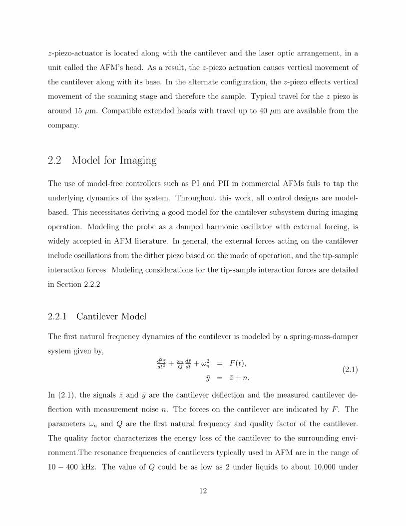
sample feature height h from the deflection measurements pm.
Figure 2.9: Cantilever transfer function Gc in feedback loop with tip-sample interaction forceFts. This viewpoint isolates nonlinear force potential Fts from the cantilever model. Thisfunction is typically bounded for the operating range of tip-sample separations.
In the AFM setup (Mfp3D from Asylum Research) used in our lab, the cantilever along
with the cantilever holder and sensing tools, including the PSD, are moved in the vertical
direction to compensate for sample inputs. Under dynamic mode of operation in this setup,
forcing on the cantilever includes the sinusoidal dither actuation g, the thermal noise η and
the tip-sample inter-atomic forces given by F (p1−h+v). The inter-atomic force is a function
of the cantilever deflection, the vertical actuation v and the sample input h. The separation
between the tip and the sample is given by (p1 − h+ v) in Mfp3D AFM configuration. The
interaction force is also a nonlinear function of the physical properties of the cantilever and
sample.
The nonlinear interaction forces are bounded for a fixed range of tip-sample separation
distance. The representation of the tip-sample dynamic model as a linear function intercon-
nected with a static non-linearity (called as Lure system in systems literature), when the
non-linearity is bounded, is very useful for model-based control design and analysis.
2.6 Proposed Control System Setup for High-speed Scanning
The model for cantilever dynamics in Section 2.5 is used as a basis to model the new imaging
mode. The cantilever transfer function is viewed to be interacting with the tip-sample forcing
Fts. Since we propose to directly use the cantilever deflection signal y for feedback, the
24
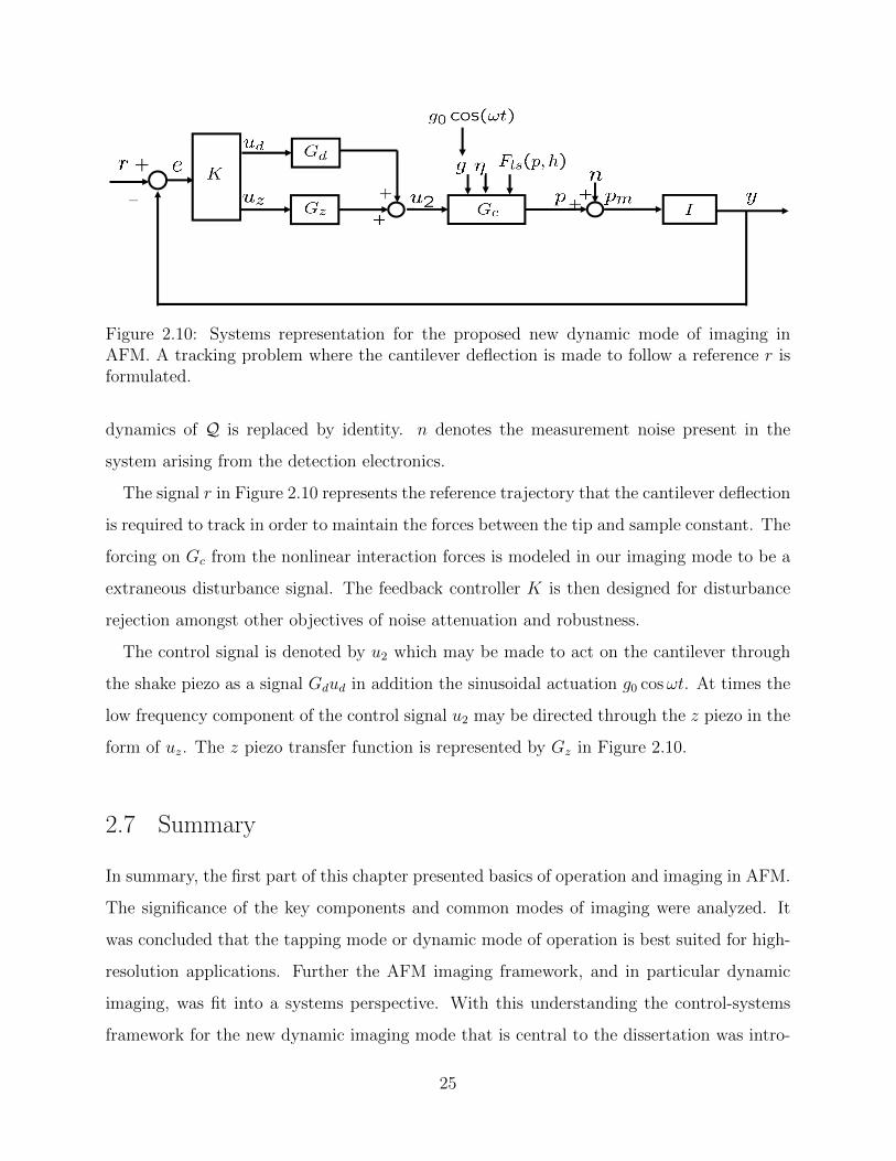
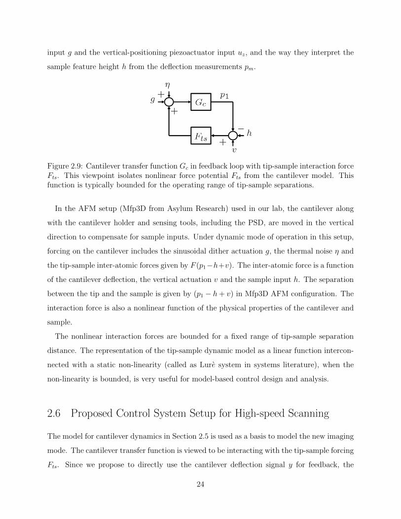
Figure 2.10: Systems representation for the proposed new dynamic mode of imaging inAFM. A tracking problem where the cantilever deflection is made to follow a reference r isformulated.
dynamics of Q is replaced by identity. n denotes the measurement noise present in the
system arising from the detection electronics.
The signal r in Figure 2.10 represents the reference trajectory that the cantilever deflection
is required to track in order to maintain the forces between the tip and sample constant. The
forcing on Gc from the nonlinear interaction forces is modeled in our imaging mode to be a
extraneous disturbance signal. The feedback controller K is then designed for disturbance
rejection amongst other objectives of noise attenuation and robustness.
The control signal is denoted by u2 which may be made to act on the cantilever through
the shake piezo as a signal Gdud in addition the sinusoidal actuation g0 cosωt. At times the
low frequency component of the control signal u2 may be directed through the z piezo in the
form of uz. The z piezo transfer function is represented by Gz in Figure 2.10.
2.7 Summary
In summary, the first part of this chapter presented basics of operation and imaging in AFM.
The significance of the key components and common modes of imaging were analyzed. It
was concluded that the tapping mode or dynamic mode of operation is best suited for high-
resolution applications. Further the AFM imaging framework, and in particular dynamic
imaging, was fit into a systems perspective. With this understanding the control-systems
framework for the new dynamic imaging mode that is central to the dissertation was intro-
25

duced. The details of this imaging technique will be presented in the following chapter.
26

CHAPTER 3
HIGH-BANDWIDTH IMAGING MODE
The high-bandwidth imaging mode proposed is effected by a model-based control design that
makes the cantilever deflection signal track a suitably designed trajectory in the dynamic
mode of operation. The reference trajectory design satisfies force regulation requirements
and ensures that the cantilever does not crash into or get completely detached from the
sample surface. The salient features of this mode of imaging are:
• It preserves the high resolution and soft forcing properties present in prevalent dynamic
modes of operation.
• The fast deflection signal of the cantilever is designed to track an appropriate trajectory
instead of regulating a derivative signal such as the amplitude or phase.
• The control effort maybe directed through the dither or shake piezo by augmenting
the sinusoidal dither signal with an additional dither control signal as well as the the
vertical piezo signal.
In Section 3.1 a model to describe the cantilever dynamics is explained, which forms
the basis for the model-based control design. Section 3.2 lays emphasis on the design of the
reference trajectory that is used to impose force regulation on the cantilever subsystem. The
forcing from the sample onto the cantilever is typically nonlinear in nature and is a function
of the tip-sample distance as well as the sample and cantilever tip properties. In our design
this force is modeled as a disturbance, thereby circumventing the problem of dealing with
a nonlinear function and subsequent nonlinear control design (see Section 3.3). The control
problem is posed, outlining the objectives, and the linear control design is described in detail
in Section 3.4.
27

dither
Figure 3.1: Spring-mass-damper model for cantilever subsystem
3.1 Model Details
In this work, the cantilever subsystem is modeled as a spring-mass-damper system with mass
m, stiffness k and damping c, as shown in Figure 3.1. The governing ODE for the model
considered is given by,
d2z
dt2+ 2ζωn
dz
dt+ ω2
nz = ω2nu+ ω2
n(g + v) +1
mFts(z − h) (3.1)
where z is the global displacement of the cantilever, ωn the first modal frequency of the
cantilever and ζ the damping coefficient (c/m = 2ζωn). The signal u denotes the control
signal driving the cantilever, and it could comprise of dither and vertical piezo actuation,
in addition to v the vertical piezo movement. The nonlinear function Fts represents the tip-
sample interaction model, which is a function of the tip position (z) and sample topography
(h). Some representative models in literature have been discussed in Section 2.2.2.
In the AFM configuration that we use, the sensing assembly moves with the cantilever.
Therefore, the signal observed by the PSD is given by
p = z − v.
Rewriting (3.1) in terms of p and using ( ˙ ) to represent ddt
, we obtain,
¨p = −2ζωn ˙p− ω2np+ ω2
ng +1
mFts(p+ v − h) + ω2
n(u− v/ω2n). (3.2)
28

The term (u− v/ω2n) is considered as the control signal to be designed and is represented by
u2 here onwards.
3.1.1 Non-dimensionalized State-space Representation
In the non-dimensionalized coordinates, the redefined time scale, τ = ωt, where ω is cho-
sen close to ωn for computational convenience.The notation ( ˙ ) implies ddτ
(). Suppose,
the sinusoidal dither signal is written as g = b cos(ωt), the redefined deflection, sample
height,vertical actuation and control signals are p = p/b, h = h/b, v = v/b and u2 = u2
respectively. The frequencies in the non-dimensionalized scale are, Ωn = ωn/ω, Ω = ω/ω.
The non-dimensionalized ODE is therefore deduced by, dividing both sides of (3.2) by ω2b
and is written as,
p = −2ζΩnp− Ω2np+ Ω2
n cos(Ωτ) +Ω2n
F0
Fts(bp+ bv − bh) + Ω2nu2. (3.3)
Here the parameter F0 = mω2nb is used for simplicity.
To derive the necessary state-space equations, p is redefined as
p1
p2
, and
p1 = p2,
p2 = −2ζΩnp2 − Ω2np1 + Ω2
n cos(Ωτ) + Ω2n
F0Fts(bp1 + bv − bh) + Ω2
nu2.(3.4)
Subsequently, defining
Ap =
0 1
−Ω2n −2ζΩn
,Bp =
0
Ω2n
,Cp =
[1 0
],
Dp = 0,
(3.5)
gives the following non-dimensionalized state-space representation for the cantilever subsys-
29
Figure 3.2: Schematic of error signal (p) dynamics G, G represents the physical cantileverdynamics and G the mock system dynamics generated on the computer.
tem model,
p = App+Bp(u2 + cos(Ωτ) + 1F0Fts), p(0) = p0
y = Cpp+ n.(3.6)
This state-space model is used as a representation of the physical cantilever subsystem for
all control design considerations from here on. In this representation the output y is the
measured deflection with measurement noise, n.
3.2 Reference Trajectory Design
A system similar to the cantilever subsystem described in (3.6) that is assumed to oscillate
over an idealized, atomically flat sample, is considered and we term it as a ‘mock system’.
The mock system inputs include sinusoidal actuation from the dither piezo and a model for
the tip-sample interaction (where the sample input is assumed to be constant). The force
model is used only in order to obtain a reasonable trajectory and does not influence the
imaging mode otherwise in a significant manner. The actual cantilever subsystem can be
thought of as the mock system augmented with forces from actual sample interactions and
the controller inputs. The mock system dynamics in the non-dimensionalized coordinates
defined in Section 3.1.1 are as follows,
30
˙p1 = p2,
˙p2 = −2ζΩnp2 − Ω2np1 + Ω2
n cos(Ωτ) + Ω2n
F0Fts(b ¯p1 − b¯h),
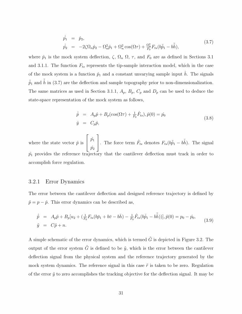
(3.7)
where p1 is the mock system deflection, ζ, Ωn Ω, τ , and F0 are as defined in Sections 3.1
and 3.1.1. The function Fts represents the tip-sample interaction model, which in the case
of the mock system is a function p1 and a constant unvarying sample input h. The signals
¯p1 and¯h in (3.7) are the deflection and sample topography prior to non-dimensionalization.
The same matrices as used in Section 3.1.1, Ap, Bp, Cp and Dp can be used to deduce the
state-space representation of the mock system as follows,
˙p = App+Bp(cos(Ωτ) + 1F0Fts), p(0) = p0
y = Cpp,(3.8)
where the state vector p is
p1
p2
. The force term Fts denotes Fts(b ¯p1 − b¯h). The signal
p1 provides the reference trajectory that the cantilever deflection must track in order to
accomplish force regulation.
3.2.1 Error Dynamics
The error between the cantilever deflection and designed reference trajectory is defined by
p = p− p. This error dynamics can be described as,
˙p = App+Bp[u2 + ( 1F0Fts(bp1 + bv − bh)− 1
F0Fts(b ¯p1 − b¯h))], p(0) = p0 − p0,
y = Cp+ n.(3.9)
A simple schematic of the error dynamics, which is termed G is depicted in Figure 3.2. The
output of the error system G is defined to be y, which is the error between the cantilever
deflection signal from the physical system and the reference trajectory generated by the
mock system dynamics. The reference signal in this case r is taken to be zero. Regulation
of the error y to zero accomplishes the tracking objective for the deflection signal. It may be
31

Figure 3.3: Closed-loop feedback diagram with G and K1, treating inter-atomic forces be-tween tip and sample as disturbance
noted that the tip-sample interaction terms are typically modeled using nonlinear functions.
3.3 Tip-Sample Interaction Forces as Disturbance
In the control design that follows, the tip-sample interaction force terms in the error dynam-
ics described in (3.9) are treated as disturbance. With G representing the error dynamics,
first a regulation problem is posed to regulate the output of the error system y (Figure 3.2)
to zero. This guarantees the tracking objective of the cantilever deflection to track the refer-
ence trajectory designed. Additionally, by modeling the interaction force as a disturbance,
the nonlinearities induced to the p and p by the tip-sample interaction is captured by the
disturbance term. The error dynamics in (3.9) can be rewritten as,
˙p = App+Bp[u2 + d], p(0) = p0 − p0,
y = Cp+ n,(3.10)
where d denotes the disturbance and is equivalent to 1F0
[Fts(bp1 + bv− bh)− Fts(b ¯p1− b¯h)]. It
may be noted that estimating this disturbance d is equivalent to estimating the tip-sample
interaction forces in the real system Fts since Fts is generated by the computer and therefore
a known quantity.
The estimation of the interaction force between the tip and sample can be used to derive
topographical as well as other physical properties of the sample. The method of estimation
is explained in Section 4.1.
32

3.4 Control Design
3.4.1 Control Objectives
The key control aim is to regulate the error y to zero through disturbance rejection. The
control objectives that are sought by the optimal controller are as follows,
• Regulation of y through disturbance rejection.
• Robust stability to any modeling uncertainties and external disturbances.
• Noise attenuation in closed-loop.
• Low effort of control.
The control design is optimized to achieve the objectives listed. The relevant closed-loop
signals required for this design are,
y = (r − n) + GSd,
em = S(r − n)− GSd,
u2 = K1S(r − n)−K1GSd,
(3.11)
where em = r − y − n, S = 1/(1 + GK1) and T = 1 − S = GK1/(1 + GK1). The error
em can be made small by designing S such that S and consequently GS are small in the
frequency regions where r, n and d are dominant. The bandwidth ωBW of S characterizes
the disturbance rejection bandwidth of the closed-loop system. Designing T to have small
roll-off frequency and high roll-off rates ensures high resolution. Robustness to external
disturbances is measured by the peak magnitude value of S. Making ||S||∞ to be close to 1
improves robustness to modeling uncertainties and disturbances. For the regulation problem
the reference signal r is set to zero.
3.4.2 Disturbance Rejection
The desired objectives are formulated in an optimal control setting based on H∞ stacked
sensitivity framework [30] (see Figure 3.4). The objectives of robust stability, disturbance
33

Figure 3.4: Closed-loop system with weighting functions for the H∞ stacked sensitivityframework
P
K
Figure 3.5: Open-loop system P in feedback with the designed controller K1
rejection and noise attenuation are realized by shaping the closed-loop transfer functions S
and T using weighting functions Ws and Wt. The weighting function Wu imposes bounded-
ness of the control signal u2. The weighted error in regulation z1 = Wsem, weighted output
z2 = Wty and weighted dither control signal z3 = Wuu2 are chosen to be the regulated
outputs. The closed-loop transfer function from w =[d r − n
]Tto z =
[z1 z2 z3
]Tis given by,
z1
z2
z3
=
−WsGS WsS
WtGS WtT
−WuT WuK1S
︸ ︷︷ ︸
Φ
d
r − n
. (3.12)
The open-loop system P with external inputs [w u2] and output z is represented as a
block diagram in Figure 3.5. From (3.12) it is observed that there are a few constraints in
34

the minimization of the closed-loop transfer function (Φ) from w to z. For instance, the
fundamental limitation S + T = I, conflicts with the simultaneous minimization of terms
WtGS and WtT . This limits the set of feasible controllers that guarantee small values of
||Φ||∞. However, the sought objectives can be accomplished by selective minimization of
certain Φ terms.
We reduce the problem to the minimization of specific transfer functions, WsGS, WsS,
WtT and WuK1S by observing that this minimization achieves closed-loop properties anal-
ogous to our desired objectives. The minimization of the transfer functions WsGS and WsS
accomplish the disturbance rejection and robustness to uncertainties objectives. The aims
of noise attenuation and low control effort are achieved through minimization of WtT and
WuK1S respectively.
Such selective minimization is made possible by the multi-objective scheme proposed
in [31]. The term −WsGS is the transfer function from d to z1 and[WsS WtT WuK1S
]Tis the transfer function from r − n to
[z1 z2 z3
]T. These constitute the cost functions
to be minimized in the multiobjective optimization problem, which is described as,
minK1∈K
γ∥∥∥WsGS
∥∥∥∞
+
∥∥∥∥∥∥∥∥∥WsS
WtT
WuK1S
∥∥∥∥∥∥∥∥∥∞
(3.13)
where γ is a parameter used to define relative importance between the two cost objectives.
The set K comprises of all the feasible stabilizing controllers K1. This multiobjective opti-
mization problem can be cast in terms of linear matrix inequalities (LMIs) [31]. Section 3.4.3
explains the details of the LMI solution formulation. The corresponding LMI conditions for
our multiobjective problem can be stated as follows: A solution to the multiobjective opti-
mization problem in (3.13) exists if there exists a solution (A, B, C, D, R, S, α1, α2) to the
optimization problem,
35
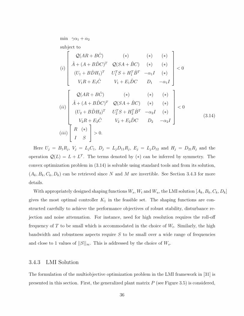
min γα1 + α2
subject to
(i)
Q(AR +BC) (∗) (∗) (∗)
A+ (A+BDC)T Q(SA+ BC) (∗) (∗)
(U1 +BDH1)T UT1 S +HT
1 BT −α1I (∗)
V1R + E1C V1 + E1DC D1 −α1I
< 0
(ii)
Q(AR +BC) (∗) (∗) (∗)
A+ (A+BDC)T Q(SA+ BC) (∗) (∗)
(U2 +BDH2)T UT2 S +HT
2 BT −α2I (∗)
V2R + E2C V2 + E2DC D2 −α2I
< 0
(iii)
R (∗)
I S
> 0.
(3.14)
Here Uj = B1Rj, Vj = LjC1, Dj = LjD11Rj, Ej = LjD12 and Hj = D21Rj and the
operation Q(L) = L + LT . The terms denoted by (∗) can be inferred by symmetry. The
convex optimization problem in (3.14) is solvable using standard tools and from its solution,
(Ak, Bk, Ck, Dk) can be retrieved since N and M are invertible. See Section 3.4.3 for more
details.
With appropriately designed shaping functionsWs, Wt andWu, the LMI solution [Ak, Bk, Ck, Dk]
gives the most optimal controller K1 in the feasible set. The shaping functions are con-
structed carefully to achieve the performance objectives of robust stability, disturbance re-
jection and noise attenuation. For instance, need for high resolution requires the roll-off
frequency of T to be small which is accommodated in the choice of Wt. Similarly, the high
bandwidth and robustness aspects require S to be small over a wide range of frequencies
and close to 1 values of ||S||∞. This is addressed by the choice of Ws.
3.4.3 LMI Solution
The formulation of the multiobjective optimization problem in the LMI framework in [31] is
presented in this section. First, the generalized plant matrix P (see Figure 3.5) is considered,
36

which takes the form,z1
z2
z3
em
=
−WsG Ws −WsG
WtG 0 WtG
0 0 Wu
−G I −G
︸ ︷︷ ︸
P
d
r − n
u2
. (3.15)
As defined in Section 3.4.2, w =[d r − n
]Tand z =
[z1 z2 z3
]T. Then state-space
realization of P is given by,
x = Ax+B1w +Bu2,
z = C1x+D11w +D12u2,
em = Cx+D21w
(3.16)
where A, B1 and B are the appropriate state-space matrices for the cantilever subsystem
model. The other system matrices follow from (3.15) and x is the system state vector. The
state-space representation of the feedback controller K1 is written as,
xk = Akxk +Bkem,
u2 = Ckxk +Dkem,(3.17)
with xk being the state vector of K1. The overall closed-loop function Φ in terms of this
state-space realization can now be computed as,
Φ =
A+BDkC BCk B1 +BDkD21
BkC Ak BkD21
C1 +D12DkC D12Ck D11 +D12DkD21
.=:
A B
C D
(3.18)
37

We seek an optimal controller of the form (3.17) that imposes H∞ performance on the
specific transfer functions,
Φ1 = WsGS,
Φ2 =[WsS WtT WuK1S
]T.
(3.19)
This allows us to follow the LMI framework adopted in [31] and [6]. Therefore, we define
the following Lj and Rj matrices for j = 1, 2,
L1 =[
1 0 0]
R1 = [ 1 0 ]T , (3.20)
L2 =
1 0 0
0 1 0
0 0 1
R2 = [ 0 1 ]T . (3.21)
The choice of the Lj and Rj matrices in (3.20) and (3.21) are such that, Φ1 = L1ΦR1 and
Φ2 = L2ΦR2. Let Uj = B1Rj, Vj = LjC1, Dj = LjD11Rj, Ej = LjD12 and Hj = D21Rj.
Also, BRj, LjC and LjDRj are denoted by Bj, Cj and Dj respectively. Then each Φj for
j = 1, 2, is
Φj =
A Bj
Cj Dj
. (3.22)
In order to impose the H∞ performance objective, we require ||Φj||∞ < αj for αj > 0. This
is equivalent to the existence of Pj > 0 such that,
ATPj + PjA (∗) (∗)
BTj Pj −αjI (∗)
Cj Dj −αjI
< 0, (3.23)
see [32]. However, this is not directly in the LMI form since the terms in (3.23) are not
linear in the variables to be designed, (Ak, Bk, Ck, Dk). In order to get LMI realization the
38

following condition is imposed,
Pj = P, (for j = 1, 2)
and the following transformations are performed. The following decomposition of the solu-
tion P is used,
P =
S N
NT ?
, P−1 =
R MT
MT ?
(3.24)
where ?s denote insignificant terms. Further we define a transformation in terms of the
following matrices
Π1 =
R I
MT 0
, Π2 =
I S
0 NT
. (3.25)
The decomposition of P in (3.24) and the fact that PP−1 = P−1P = I implies MNT =
I −RS, PΠ1 = Π2. The redefined variables,
A = NAkMT +NBkCR + SBCkM
T
+S(A+BDkC)R, (3.26)
B = NBk + SBDk,
C = CkMT +DkCR,
D = Dk,
are used to formulate the optimization problem in terms of LMIs. Upon imposing H∞performance on both φ1 and φ2, we get equations of the form shown in (3.23). Through
appropriate congruent transformations diag(Π1, I, I), the LMI conditions (i) and (ii) in (3.14)
are deduced. Subsequently, ΠT1 PΠ1 gives the inequality condition (iii) in (3.14).
From the optimized variables (A, B, C, D, R, S), with M and N being invertible, the
39

matrices (Ak, Bk, Ck, Dk) are got as follows:
Ak = N−1(A− (B − SBD)CR− SB(C − DCR)
−S(A+BDC)R)M−T
Bk = N−1(B − SBD)
Ck = (C − DCR)M−T
Dk = D
(3.27)
The state-space matrices (Ak, Bk, Ck, Dk) represent the optimal controller K1 for the can-
tilever model.
3.4.4 Choice of Weighting Functions
Appropriate design of the weighting functions, Ws, Wt, and Wu (from Figure 3.4) is crucial
for achieving the desired control objectives. In the stacked sensitivity framework, the loop
transfer function GcK1 is shaped by designing closed-loop functions, namely the sensitivity
function S and complementary sensitivity function T as desired. Imposing ||WsS||∞ < 1 on
the design of S applies a lower bound on the bandwidth of the closed-loop system. An upper
bound is applied to the magnitude of the function T through 1/|Wt| ensuring that the loop
transfer function rolls off sufficiently fast at higher frequencies beyond the frequency region
of interest. And the weighting function Wu is used to limit the magnitude of control input
signals to 1/|Wu|.
A cantilever subsystem with a natural frequency of 69.578 kHz, stiffness k of 1.43, and
damping ζ = 0.0033 was considered for the following choice of weighting functions. The sys-
tem equations are normalized as described in Section 3.1 with ω = ωn and b = 2.9155 nm.
For the design of the controller K1, the shaping functions, Ws = 0.3(s+35.93)s+0.1078
, Wt = 100(s+3.593)s+1078
and Wu = 0.1 were chosen to capture the performance objectives of high bandwidth, resolu-
tion and robustness to disturbances. The choice of these transfer functions is dependent on
the specific system properties and requirements. The sensitivity function S is designed to be
small in a wide range of frequencies where the signals r and d are dominant. However, the
reference signal in our regulation problem r is chosen to be zero and Ws is chosen to have a
40
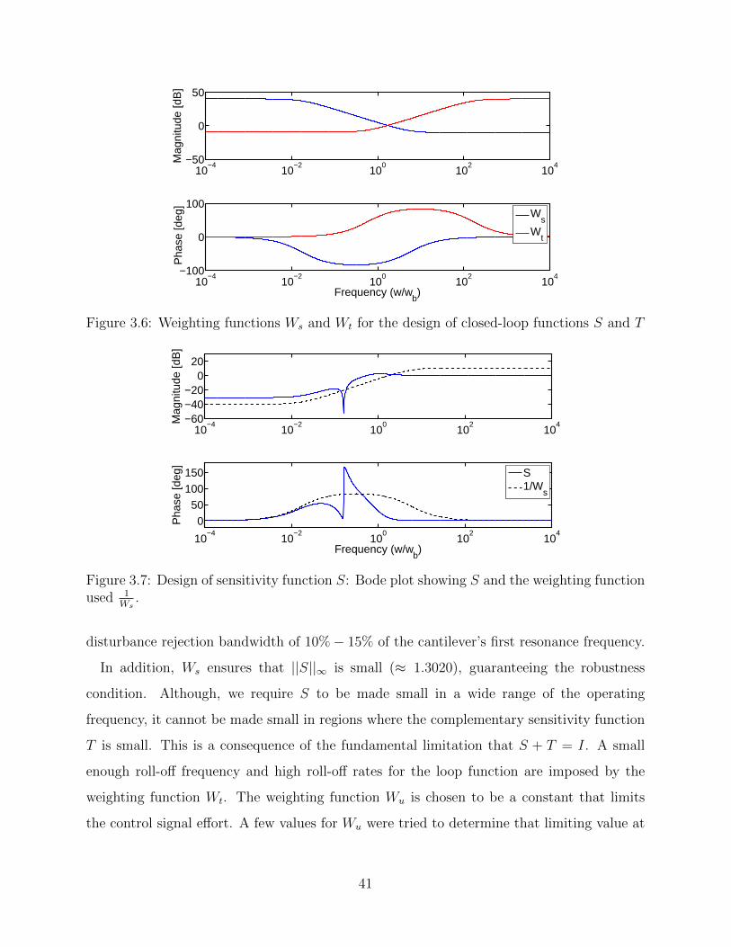
10−4
10−2
100
102
104−50
0
50
Mag
nitu
de [d
B]
10−4
10−2
100
102
104−100
0
100
Pha
se [d
eg]
Frequency (w/wb)
Ws
Wt
Figure 3.6: Weighting functions Ws and Wt for the design of closed-loop functions S and T
10−4
10−2
100
102
104−60
−40−20
020
Mag
nitu
de [d
B]
10−4
10−2
100
102
104
050
100150
Pha
se [d
eg]
Frequency (w/wb)
S1/W
s
Figure 3.7: Design of sensitivity function S: Bode plot showing S and the weighting functionused 1
Ws.
disturbance rejection bandwidth of 10%− 15% of the cantilever’s first resonance frequency.
In addition, Ws ensures that ||S||∞ is small (≈ 1.3020), guaranteeing the robustness
condition. Although, we require S to be made small in a wide range of the operating
frequency, it cannot be made small in regions where the complementary sensitivity function
T is small. This is a consequence of the fundamental limitation that S + T = I. A small
enough roll-off frequency and high roll-off rates for the loop function are imposed by the
weighting function Wt. The weighting function Wu is chosen to be a constant that limits
the control signal effort. A few values for Wu were tried to determine that limiting value at
41

10−4
10−2
100
102
104−200
−100
0
Mag
nitu
de [d
B]
10−4
10−2
100
102
104−200
−100
0
Pha
se [d
eg]
Frequency (w/wb)
T1/W
t
Figure 3.8: Design of complementary sensitivity function T : Bode plot showing T and theweighting function used 1
Wt.
which the optimization fails. This parameter limits the set of feasible controllers considered
during optimization.
10−4
10−2
100
102
104−200
−100
0
Mag
nitu
de [d
B]
10−4
10−2
100
102
104−200
−100
0
Pha
se [d
eg]
Frequency (w/wb)
GcK
1
Figure 3.9: Magnitude and phase plots of the loop transfer function L = GK1. The weightingfunctions limit the peak value and define the roll-off rates at high frequencies.
Bode plots of Ws and Wt are illustrated in Figure 3.6. This is followed by plots of the
designed closed-loop transfer functions S and T in Figures 3.7 and 3.8 respectively. The
weighting functions 1/Ws and 1/Wt are shown in black dotted lines. The performance of
the optimization solution can be seen from these plots. In all the magnitude and phase plots
in this section, the logarithmic frequency axis has no units owing to non-dimensionalization
using ω (denoted by wb in the plots).
42

10−4
10−2
100
102
104−200
−100
0
Mag
nitu
de [d
B]
10−4
10−2
100
102
104−200
0
200
Pha
se [d
eg]
Frequency (w/wb)
Figure 3.10: Magnitude and phase plots of the closed-loop transfer function GcS
10−10
10−5
100
105
1010
1015−100
−50
0
Mag
nitu
de [d
B]
10−10
10−5
100
105
1010
1015−200
0
200
Pha
se [d
eg]
Frequency (w/wb)
K1S
Figure 3.11: Magnitude and phase plots of the the closed-loop transfer function K1S
3.4.5 Minimization Solution
In Figure 3.12 a table showing the infinity-norm values of the elements in the closed-loop
matrix Φ in (3.12) are presented along with the corresponding plot depicting the same. The
terms are shown as Φij where i and j denote the row and column of the elements in the
matrix respectively. The minimization problem with the given transfer function choices for
Ws, Wt and Wu yields ||Φ1||∞ = 3.4535 and ||Φ2||∞ = 3.4587, where Φ1 and Φ2 are defined
in (3.19). The controller K1 after minimal realization is computed to be,
K1 =2.357× 10¹²s3 + 2.543× 10¹⁵s2 + 2.026× 10¹⁵s+ 2.899× 10¹⁵
s4 + 6.84× 10¹⁰s3 + 7.436× 10¹³s2 + 6.616× 10¹⁴s+ 7.045× 10¹³. (3.28)
43

||Φ||∞ valuesΦ11 3.4535Φ12 3.3300Φ21 0.1192Φ22 3.4456Φ31 0.1126Φ32 0.5063
1112 2122 31320
1
2
3
4
Φ terms
Infin
ity n
orm
Figure 3.12: ||.||∞ norms of the terms in closed-loop matrix Φ (see (3.12)) upon minimization.The subscripts denote the position of the element in the matrix.
The magnitude and phase characteristics of the resultant loop transfer function GK1 is shown
in Figure 3.9. The high roll-rates at higher frequencies is a consequence of the Wt design.
It must be noted that as a result of non-dimensionalization, 100 on the frequency axis cor-
responds to the first resonance frequency of the cantilever. Closed-loop simulations of the
1400 1500 1600−0.5
0
0.5
1
1/2π cycles
h(τ
)
(a)
1450 1500 1550 1600−2
0
2
4
1/2π cycles
y
(b)
Figure 3.13: (a) shows the normalized height profile with frequency ωhω
= 0.1 and amplitudeahb
= 0.4. (b) The regulating action of the controller K1 makes y = p1 settle to zero withina cycle after every tip-sample interaction. These interactions are in the form of impulses,causing instantaneous state jumps of p1 as seen in this plot of y.
controller K1 in feedback with the error subsystem G were performed on Matlab Simulink.
The normalized sinusoidal sample profile shown in Figure 3.13(a), whose amplitude is ah/b
and frequency is ωh/ω . The DMT model was chosen to model the tip-sample interaction
forcing in the systems G and G, which has been widely corroborated in literature [4], [33].
The tip sample interaction d occurs in the form of impulses, each time the cantilever inter-
44

1450 1500 1550 1600
0
50
100
150
1/2π cycles
d
(a)
1530 1532 1534
0
50
100
150
1/2π cycles
d
(b)
Figure 3.14: (a) The forcing from the tip sample interaction occurs as an impulse resulting ininstantaneous value change of p1 and hence p. When the cantilever is within a small distancefrom the sample, the interaction force impulses occur once every period of oscillation asshown in (b). Note that the x-axis shows 1
2πcycles.
acts with the sample, p1 assumes a different value instantaneously when this happens (see
Figures 3.14(a), 3.14(b)). The magnitude of the resultant disturbance signal d is maintained
small by the design of d. However, it is not required for the mock system to have a distur-
bance signal d as long as the amplitude of the reference trajectory is appropriately generated
to effect the desired forcing on the sample and satisfy force regulation.
It can be been observed that the interaction force d occurs as impulses or spikes (see
Figure 3.14(a). This is because the cantilever spends only a small fraction of each cycle in
contact (i.e. within atomic scale separation) with the sample surface. Therefore, reducing
the amplitude of oscillation of the cantilever will increase the time spent in contact with the
sample thereby making the impulse like forcing smoother. But very low amplitudes could
cause the cantilever to remain in attractive force region during most of its oscillation causing
it to snap on to the surface.
The cantilever is made to stay predominantly in the repulsive region in accordance to
dynamic mode of imaging in AFM. Furthermore, the regulating action of controller K1
brings p1 to p1 or equivalently p to 0 within a cycle as seen in Figure 3.13(b). As long as the
effective sample spatial frequency is within 15− 20% of the cantilever resonance frequency,
force regulation is attained [34]. However, this does not limit the bandwidth of sample
45
property or topography estimation as will be seen in Chapter 4. The loop shaping is done
for the best possible force regulation bandwidth, i.e. disturbance rejection bandwidth.
3.5 Summary
The control system perspective from Chapter 2 was adopted and cantilever dynamics were
modeled in accordance to this systems setup. A tracking problem on the cantilever deflection
to achieve force regulation was successfully formulated, followed by design of a H∞-based
controller that regulates the tracking error to zero. The step-by-step details of construct-
ing this regulating controller were discussed. Finally, the favorable performance results on
simulations were presented. In the following chapter methods to estimate the rejected dis-
turbance, followed by sample property estimation are discussed.
46

CHAPTER 4
SAMPLE PROPERTY ESTIMATION
Separation of the goals of force regulation and force estimation, allows for a high disturbance
estimation bandwidth. This is explored in this chapter by designing a controller that acts
upon the output of the error subsystem G from Section 3.2.1. It has already been established
that current amplitude modulation techniques or tapping mode operation do not suffice for
high-speed operations, because of change in cantilever amplitude even within a cycle of its
oscillation. As a consequence, the current methods of sample topography estimation directly
using the control signal are also erroneous at high-speeds.
The proposed dynamic mode of imaging compensates for the effect of forcing from the
sample through force regulation. Furthermore, in place of estimating the sample topography,
a transfer function that can estimate the forces due to sample interaction is sought, which
gives a more direct/raw form of data. Design for disturbance estimation is given in Sec-
tion 4.1. Methods to use the force data to obtain sample topography estimates are discussed
in Section 4.2.2. In order to get the physical properties of sample from the force estimates, it
is important to understand typical forcing models. Using these models as reference a generic
force model is adopted and a few example techniques to deduce sample properties using this
generic model are shown in Section 4.2.3.
4.1 Disturbance Estimation
This section deals with the design of controller K2 (see Figure 4.1) such that, ˆd = K2em
gives an estimate of the tip sample interaction force difference d. In the AFM setup, the
deflection p1 is measurable from sensors, and p1 is also known since it is a state of the mock
47

Figure 4.1: The controller K2 used to estimate the disturbance d from the regulation error
signal em, highlighted by the blue box. The estimate is denoted by ˆd and the estimationerror by ed.
system. An estimate of d can be numerically obtained from y since,
y = p1 − p1 = GSd. (4.1)
Therefore, S−1G−1y is an estimate of d when S is a minimum phase transfer function.
10−4
10−2
100
102
1040
50
100
Mag
nitu
de [d
B]
10−4
10−2
100
102
104−100
0
100
Pha
se [d
eg]
Frequency (w/wb)
K2
Figure 4.2: Bode diagram of the force estimating controller K2
However, when the transfer function is non-minimum phase, the Nevanlinna-Pick method
can be adopted to design an appropriate inverse transfer function through a minimization
problem [35]. Furthermore, we append a stable second-order low-pass filter Ψ, whose cut-off
frequency ωF is larger than the resonance frequency and therefore larger than the highest
frequency component of h considered. This guarantees that the transfer function from n to
48
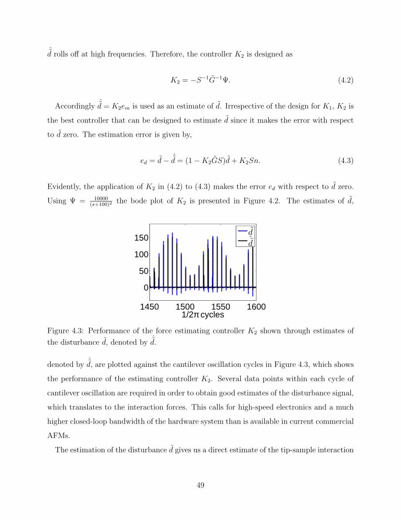
ˆd rolls off at high frequencies. Therefore, the controller K2 is designed as
K2 = −S−1G−1Ψ. (4.2)
Accordingly ˆd = K2em is used as an estimate of d. Irrespective of the design for K1, K2 is
the best controller that can be designed to estimate d since it makes the error with respect
to d zero. The estimation error is given by,
ed = d− ˆd = (1−K2GS)d+K2Sn. (4.3)
Evidently, the application of K2 in (4.2) to (4.3) makes the error ed with respect to d zero.
Using Ψ = 10000(s+100)2
the bode plot of K2 is presented in Figure 4.2. The estimates of d,
1450 1500 1550 1600
0
50
100
150
1/2π cycles
dˆd
Figure 4.3: Performance of the force estimating controller K2 shown through estimates of
the disturbance d, denoted by ˆd.
denoted by ˆd, are plotted against the cantilever oscillation cycles in Figure 4.3, which shows
the performance of the estimating controller K2. Several data points within each cycle of
cantilever oscillation are required in order to obtain good estimates of the disturbance signal,
which translates to the interaction forces. This calls for high-speed electronics and a much
higher closed-loop bandwidth of the hardware system than is available in current commercial
AFMs.
The estimation of the disturbance d gives us a direct estimate of the tip-sample interaction
49

force of the real cantilever subsystem. Since,
d = d− d,
and d is a part of the mock system generated digitally, ˆd can be reduced to estimates of d,
which in turn represents Fts(p1−h+v). Therefore, the design of K2 facilitates the estimates
of the tip-sample interaction forces. These estimates can be further fit with force models to
compute the specific physical sample properties of interest.
4.2 Topography and Property Estimation
Force curves, which are plots of the interaction force against the tip-sample separation are
used to obtain property estimates of the sample. Force modulation techniques were devel-
oped for samples with variations in local surface elasticity [36]. The variation in elasticity
is measured by the changes in cantilever deflection under constant average force. In [37],
the authors use a series of approach-retract force curves to obtain time series data of the
cantilever response and thereby identify the cantilever transfer function. Here, small oscil-
lation amplitudes are considered and the nonlinear tip-sample interaction force is assumed
to be linearized and absorbed as a system internal parameter. Experiments in low damp-
ing environments have also been used to estimate the relationship between the cantilever
frequency shift and the interaction potential [38]. Majority of these techniques utilize force
curves taken at discrete locations on the sample quiasi-statically and map them to physical
properties. Although they are effective in estimating sample properties, they suffer from
the disadvantages of long process time and limitations in the spatial/lateral resolution of
the sample properties. Some other techniques like the contact-resonance AFM [39] estimate
the visco-elastic properties of the sample without estimating the interaction forces, assum-
ing a spring-dashpot tip-sample interaction model. The excitation of the cantilever at two
frequencies (close to its natural frequency) in addition to oscillating it at resonance in tap-
ping mode has been shown to estimate equivalent cantilever parameters at higher speeds
than conventional techniques [40]. However, a simple model is assumed for the tip-sample
50

interaction.
Our high bandwidth imaging technique along with K2 provides dynamic estimates of
the tip-sample force as against the static methods predominantly used to estimate sample
properties. A brief discussion of the Hertz (short range repulsive force), DMT, JKR and
Maugis models for inter-atomic forces between surfaces is presented to motivate the use of a
generic force model. This generic model has been fit to the force estimates obtained through
the design of K2.
4.2.1 Generic Force Model
Under the Hertz contact force model a frictionless contact without any forces of adhesion is
assumed. It is appropriate for high normal loads or low surface forces. The force equations
in the Hertz model are given by,
Fts =
0 zts > 0
43E∗√R(−zts)
32 zts ≤ 0
, (4.4)
where R is the tip radius, and E∗ = ((1−ν2t )
Et+ (1−ν2s )
Es)−1 is the effective Young’s modulus of
the tip and sample. Individual Young’s moduli and Poisson’s ratios are represented by E
and ν, with subscripts s and t referring to the sample and tip respectively.
DMT, JKR as well as the Maugis model are based off of the Hertz model with the addition
of long range attractive Van der Waals forces. The JKR model [27] applies to highly adhesive
systems with low stiffness and large tip radii, translating to compliant materials with strong
adhesion properties and a blunt tip. It assumes a non-zero contact area at zero load. The
contact radius at separation is modeled to be 0.63a0, where a0 is the intermolecular distance.
This model predicts instability during approach and retraction of tip to or from a sample
surface. During loading it models a neck forming between the tip or sample, contributing to
hysteresis.
The DMT model constraints the tip-sample geometry to be Hertzian [4]. Finite stresses
at contact perimeter and surface forces acting outside the contact region are considered. It
51

is best suited for rigid systems with small adhesion forces and sharp tips. The governing
equations are given by,
Fts =
−HR6z2ts
zts > a0
−HR6a20
+ 43E∗√R(a0 − zts)
32 zts ≤ a0
, (4.5)
where H is the Hamaker’s constant dependent on the materials in contact.
The Maugis model lies in the spectrum between JKR and DMT models in terms of ad-
hesion force influence. A variable parameter λ is used to define the adhesion force influence
in the model. When this λ = 0 in Maugis model, it results in the Hertz model, λ < 0.1
gives the DMT model and λ > 5 results in the JKR model. The models described are often
modified or additional terms are added depending on the operating conditions.
In our formulation for property estimation, these models are taken as a basis and a generic
model is described as follows. The tip-sample interaction force in the attractive and repulsive
regions,
Fts(zs) =
α(a0 − zs)m zs < 0
β + γ(zs)n zs ≥ 0
, (4.6)
where α, β and γ are parameters governed by the properties of the interacting materials,
and zs = a0−zts, with a0 being the intermolecular distance and zts is the separation between
probe-tip and sample. For instance, in case of the DMT model equations in (4.5), α = −HR6
,
β = −HR6a20
, γ = 43E√R, and m = −2 and n = 3/2. This generic model will be employed in
Section 4.2.3 where methods to derive estimates of sample physical properties are elucidated.
It is very important to note that the force models described here are merely used to
develop a generic model that can be used to fit the force data with. The imaging mode
measures the interaction forces which comprise all the properties of the sample. Therefore,
the mode facilitates access to the most basic information available about the sample. Any
property inferred from this data implies underlying assumptions inherent in the model used
for interpreting the estimates.
52

4.2.2 Topography Estimates
As a next step, some relations are presented that enable the estimation of the sample to-
pography from the estimate ˆd. The nonlinear force of the tip-sample interaction in terms of
the separation between the tip and the sample is piecewise continuous and bounded for a
practical range of separation distances. On application of mean value theorem the forcing
term,
F (bp1 − bh+ bv)− F (bp1 − bh) = Θ(τ)(bp1 − bh− bv), (4.7)
where Θ = ∂F∂z
with z lying between (bp1− bh+ bv) and (bp1− bh). We can assume that the
sample topography (h) is approximately a constant over a period of cantilever oscillation
and the integral of p1 is negligible owing to its small values. With these assumptions and
v = 0 we get, ∫ T
T− 2πO
[F (bp1 − bh)− F (bp1)]dτ =
∫ T
T− 2πO
Θ(τ)dτ(bh). (4.8)
1400 1500 1600−1
0
1
2
1/2π cycles
hh
(a)
1400 1500 1600−2
0
2
4
1/2π cycles
hh
(b)
Figure 4.4: (a) and (b) show the estimates of a sinusoidal sample profile through the to-pography estimation. The blue lines indicate the sample profile considered while the dottedlines show the estimates.
Therefore, integration of the estimate ˆd over every period of cantilever oscillation, facili-
tates the estimation of the height signal h(τ). It may be noted that the z-piezo actuation
signal v can be designed to keep d within the estimation bandwidth of K2, but this is not
analyzed in this paper.
It is important to note that all plots contain non-dimensionalized values unless otherwise
53
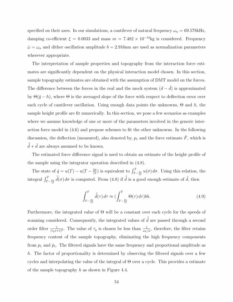
specified on their axes. In our simulations, a cantilever of natural frequency ωn = 69.578kHz,
damping co-efficient ξ = 0.0033 and mass m = 7.482 × 10⁻¹²kg is considered. Frequency
ω = ωn and dither oscillation amplitude b = 2.916nm are used as normalization parameters
wherever appropriate.
The interpretation of sample properties and topography from the interaction force esti-
mates are significantly dependent on the physical interaction model chosen. In this section,
sample topography estimates are obtained with the assumption of DMT model on the forces.
The difference between the forces in the real and the mock system (d− d) is approximated
by Θ(y− h), where Θ is the averaged slope of the force with respect to deflection error over
each cycle of cantilever oscillation. Using enough data points the unknowns, Θ and h, the
sample height profile are fit numerically. In this section, we pose a few scenarios as examples
where we assume knowledge of one or more of the parameters involved in the generic inter-
action force model in (4.6) and propose schemes to fit the other unknowns. In the following
discussion, the deflection (measured), also denoted by, p1 and the force estimate F , which is
ˆd+ d are always assumed to be known.
The estimated force difference signal is used to obtain an estimate of the height profile of
the sample using the integrator operation described in (4.8).
The state of q = u(T )− u(T − 2πO
) is equivalent to∫ TT− 2π
Ou(σ)dσ. Using this relation, the
integral∫ TT− 2π
O
ˆd(σ)dσ is computed. From (4.8) if ˆd is a good enough estimate of d, then
∫ T
T− 2πO
ˆd(τ)dτ ≈ (
∫ T
T− 2πO
Θ(τ)dτ)bh. (4.9)
Furthermore, the integrated value of Θ will be a constant over each cycle for the speeds of
scanning considered. Consequently, the integrated values of ˆd are passed through a second
order filter 1(τqs+1)2
. The value of τq is chosen be less than 1ωh/ω
, therefore, the filter retains
frequency content of the sample topography, eliminating the high frequency components
from p1 and p1. The filtered signals have the same frequency and proportional amplitude as
h. The factor of proportionality is determined by observing the filtered signals over a few
cycles and interpolating the value of the integral of Θ over a cycle. This provides a estimate
of the sample topography h as shown in Figure 4.4.
54
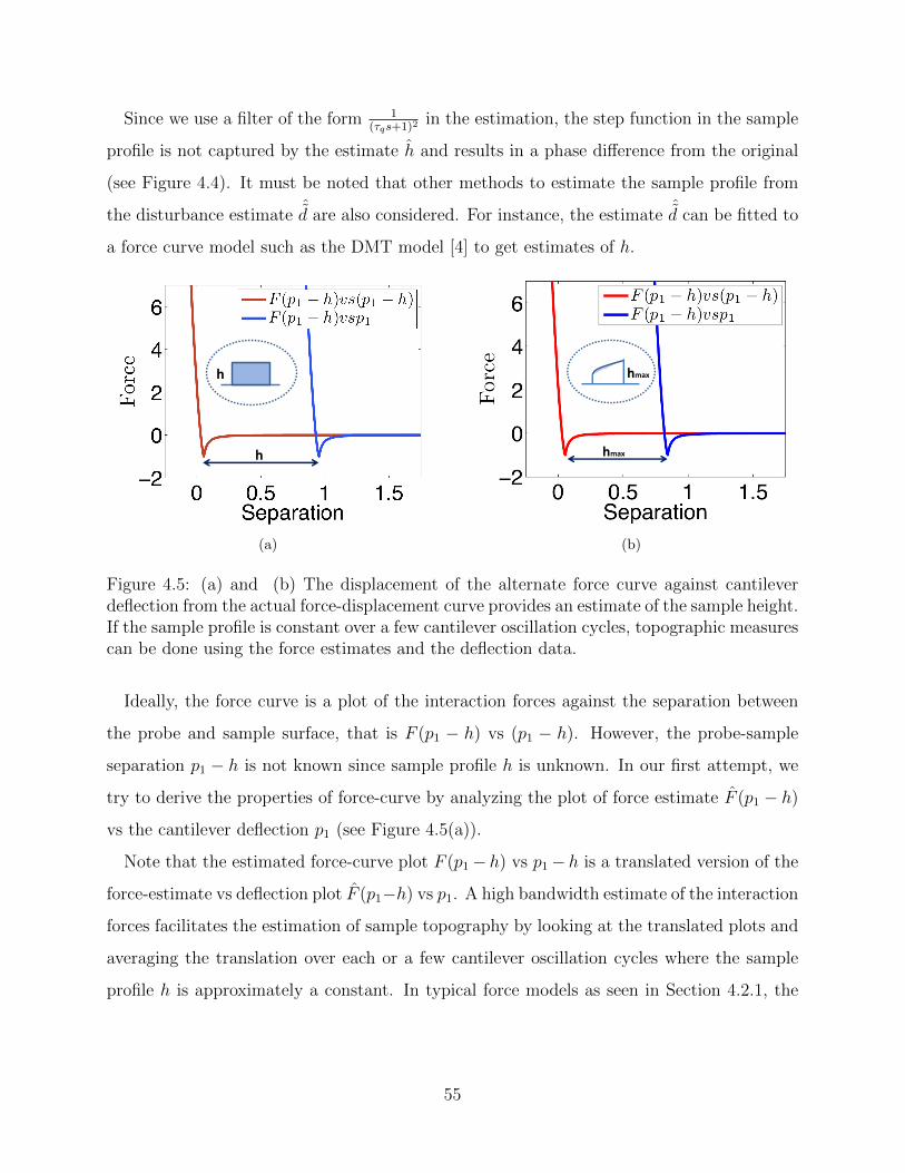
Since we use a filter of the form 1(τqs+1)2
in the estimation, the step function in the sample
profile is not captured by the estimate h and results in a phase difference from the original
(see Figure 4.4). It must be noted that other methods to estimate the sample profile from
the disturbance estimate ˆd are also considered. For instance, the estimate ˆd can be fitted to
a force curve model such as the DMT model [4] to get estimates of h.
!"
!"
(a)
(b)
Figure 4.5: (a) and (b) The displacement of the alternate force curve against cantileverdeflection from the actual force-displacement curve provides an estimate of the sample height.If the sample profile is constant over a few cantilever oscillation cycles, topographic measurescan be done using the force estimates and the deflection data.
Ideally, the force curve is a plot of the interaction forces against the separation between
the probe and sample surface, that is F (p1 − h) vs (p1 − h). However, the probe-sample
separation p1 − h is not known since sample profile h is unknown. In our first attempt, we
try to derive the properties of force-curve by analyzing the plot of force estimate F (p1 − h)
vs the cantilever deflection p1 (see Figure 4.5(a)).
Note that the estimated force-curve plot F (p1− h) vs p1− h is a translated version of the
force-estimate vs deflection plot F (p1−h) vs p1. A high bandwidth estimate of the interaction
forces facilitates the estimation of sample topography by looking at the translated plots and
averaging the translation over each or a few cantilever oscillation cycles where the sample
profile h is approximately a constant. In typical force models as seen in Section 4.2.1, the
55
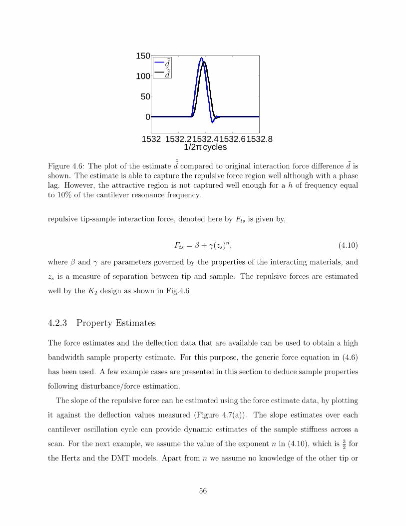
1532 1532.21532.41532.61532.8
0
50
100
150
1/2π cycles
dˆd
Figure 4.6: The plot of the estimate ˆd compared to original interaction force difference d isshown. The estimate is able to capture the repulsive force region well although with a phaselag. However, the attractive region is not captured well enough for a h of frequency equalto 10% of the cantilever resonance frequency.
repulsive tip-sample interaction force, denoted here by Fts is given by,
Fts = β + γ(zs)n, (4.10)
where β and γ are parameters governed by the properties of the interacting materials, and
zs is a measure of separation between tip and sample. The repulsive forces are estimated
well by the K2 design as shown in Fig.4.6
4.2.3 Property Estimates
The force estimates and the deflection data that are available can be used to obtain a high
bandwidth sample property estimate. For this purpose, the generic force equation in (4.6)
has been used. A few example cases are presented in this section to deduce sample properties
following disturbance/force estimation.
The slope of the repulsive force can be estimated using the force estimate data, by plotting
it against the deflection values measured (Figure 4.7(a)). The slope estimates over each
cantilever oscillation cycle can provide dynamic estimates of the sample stiffness across a
scan. For the next example, we assume the value of the exponent n in (4.10), which is 32
for
the Hertz and the DMT models. Apart from n we assume no knowledge of the other tip or
56

0 2 40
20
40
60
(p1−h)
FF
(a)
0 2 40
50
100
150
200
(p1−h)
FF
(b)
−8 −7 −6 −5x 10⁻¹⁰
2468
x 10−6
a0 − bp1 (m)
(F−β
)(1/n
) (N
)
dxdy
(c)
Figure 4.7: (a) The force F corresponds to the forcing term used in our simulations for thereal system and F corresponds to the estimate obtained. The phase lag in the estimateof d (Figure 4.6) is reflected in the plot of forces against the corresponding separations forsample. (b) shows the same for a constant sample surface. (c) The plot shows the left handside of (4.11) plotted against the values of a0− p1 that are available through estimation andmeasurement. The slope of the plot corresponds to the value of ψ = γ2/3.
sample properties. In this case, (4.10) can be re-written as,
(Fts − β)2/3 = (γ)2/3(zs),
= ψ(a0 − p1) + ψ(h),(4.11)
where we denote γ2/3 by ψ, a0 is the intermolecular distance and the separation zs = a0 −
p1 − h. From (4.10), it is observed that the parameter β is the minimum value of the
repulsive force with respect to the tip-sample separation distances. This can be computed
numerically using the available interaction force estimate F = ˆd − F (p1) within an error
57
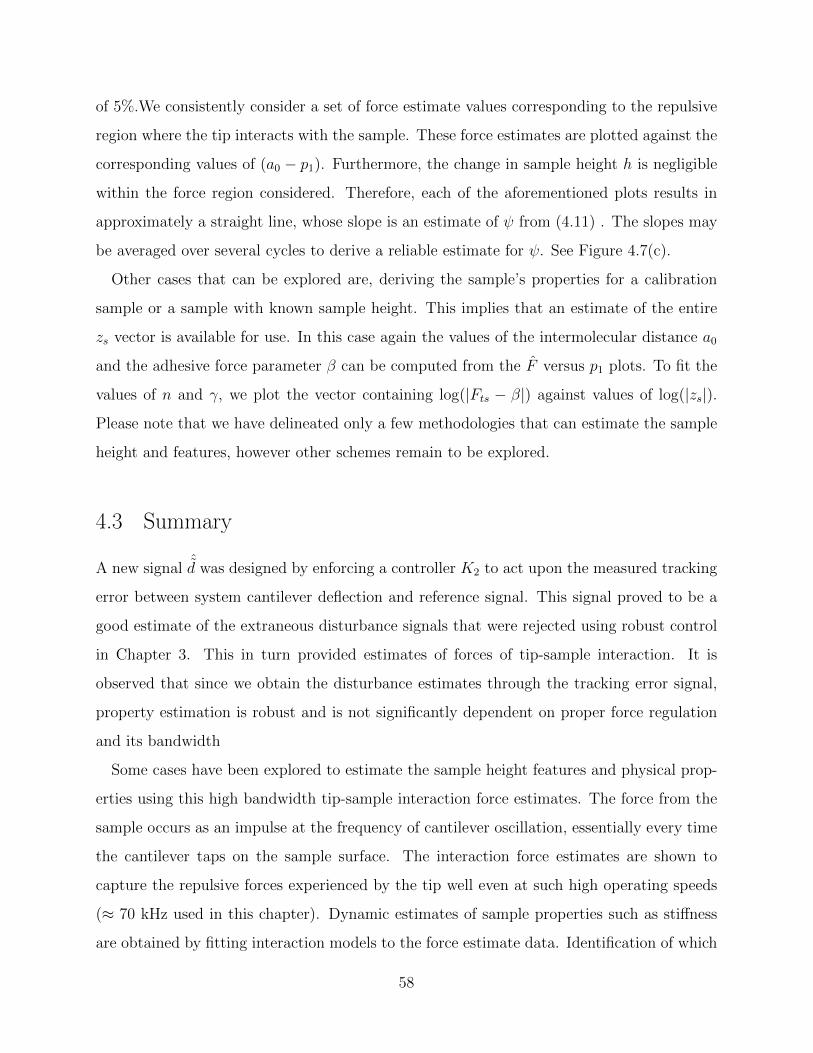
of 5%.We consistently consider a set of force estimate values corresponding to the repulsive
region where the tip interacts with the sample. These force estimates are plotted against the
corresponding values of (a0 − p1). Furthermore, the change in sample height h is negligible
within the force region considered. Therefore, each of the aforementioned plots results in
approximately a straight line, whose slope is an estimate of ψ from (4.11) . The slopes may
be averaged over several cycles to derive a reliable estimate for ψ. See Figure 4.7(c).
Other cases that can be explored are, deriving the sample’s properties for a calibration
sample or a sample with known sample height. This implies that an estimate of the entire
zs vector is available for use. In this case again the values of the intermolecular distance a0
and the adhesive force parameter β can be computed from the F versus p1 plots. To fit the
values of n and γ, we plot the vector containing log(|Fts − β|) against values of log(|zs|).
Please note that we have delineated only a few methodologies that can estimate the sample
height and features, however other schemes remain to be explored.
4.3 Summary
A new signal ˆd was designed by enforcing a controller K2 to act upon the measured tracking
error between system cantilever deflection and reference signal. This signal proved to be a
good estimate of the extraneous disturbance signals that were rejected using robust control
in Chapter 3. This in turn provided estimates of forces of tip-sample interaction. It is
observed that since we obtain the disturbance estimates through the tracking error signal,
property estimation is robust and is not significantly dependent on proper force regulation
and its bandwidth
Some cases have been explored to estimate the sample height features and physical prop-
erties using this high bandwidth tip-sample interaction force estimates. The force from the
sample occurs as an impulse at the frequency of cantilever oscillation, essentially every time
the cantilever taps on the sample surface. The interaction force estimates are shown to
capture the repulsive forces experienced by the tip well even at such high operating speeds
(≈ 70 kHz used in this chapter). Dynamic estimates of sample properties such as stiffness
are obtained by fitting interaction models to the force estimate data. Identification of which
58

properties can be estimated robustly is dependent on the choice of model and experimental
conditions.
59

CHAPTER 5
EXPERIMENTAL RESULTS
Preliminary experiments were conducted to validate performance of the controllers that have
been verified through simulations. The issues confronted in the process of implementation
and the results obtained are explained in this chapter. The roadblocks faced during attempts
for in-air imaging are briefed in Section 5.1. Section 5.2. The controller design is revised
for in-water imaging, and this is presented in Section 5.2.1 Also, differences in imaging in
the two media are briefed. The experimental set up including the system transfer functions
identified for in-water imaging case are explained in Section 5.2.2.
5.1 Imaging in Air: Issues
In the ideal case, experiments with tapping mode cantilevers with resonance frequencies in
the order of 100−300 kHz would have been performed. The functional electronics in our lab
does not accommodate operating in the closed-loop with data of such high frequency orders.
Installing new FPGA-based electronics hardware and learning the programming know-how
was not feasible in stipulated time.
While using AFM as a tool, there is no advantage to using a low frequency tip for dynamic
mode imaging in air. The tapping mode cantilever market is gravitating towards mega Hertz
resonance frequencies for reasons quoted in Section 1.2.1. Typically, contact mode cantilevers
are the ones that lie in low frequency spectrum. However, the stiffness of these cantilevers
are inadequate for scanning in air. This results in insufficient forcing and therefore spurious
images while scanning.
During imaging, a fluid cell or water droplet can be used to immerse a contact mode
cantilever and holder. Under water, the typical stiffness values of such cantilevers (0.15 −
60

0.35 N/m) render good images. Moreover, the resonance frequency of the cantilever shifts
to a lower value (≈ 13
is the factor of reduction for water) when immersed in a fluid. This is
accounted for by the viscosity of the fluid used [41]. The quality of the SiNi probes used for
our experiments is not large, but with enough forcing good quality images were possible.
5.2 Imaging in Fluids: Proof of Concept
After consideration of options for low frequency operation in air, it was concluded that
imaging in water was a good alternative. In this set up, frequencies that are within the
capabilities of DSP hardware are possible in addition to rendering reliable and quality imag-
ing. The objective is to demonstrate the validity of force regulation using deflection tracking
(to a trajectory y) through disturbance rejection control. Before proceeding to the control
design it is important to understand the behavior of the cantilever while imaging in water.
For the same cantilever, the properties in air and water differ considerably except for the
stiffness that remains almost unchanged. Figure 5.1 shows the unforced thermal response for
a cantilever of stiffness ≈ 2 N/m. The thermal response shows first natural frequency of this
cantilever to be around 32 kHz when in air at a given temperature. The resonance frequency
lowers by a factor of about 13
when placed in water, as shown in the thermal response in
Figure 5.1(b). Furthermore, owing to increased damping (goes from 0.014 to 0.152 in for
sample cantilever considered) the quality factor (Q) decreases considerably.
The quality factor is defined by,
Q =ωn∆ω
,
where ∆ω is the half-power bandwidth i.e. the bandwidth over which the power of vibration
is greater than half the power at the resonant frequency. This explains the broader peak of
the cantilever response when used in water.
In order to determine the precise drive frequency of cantilever operation, a drive frequency
sweep is performed by the shake piezo in a bandwidth around the resonant peak identified
from the thermal response. For imaging in air, this peak is distinctly seen during the drive
frequency sweep or tune process (see Figure 5.2(a). It is observed that traditionally in
61
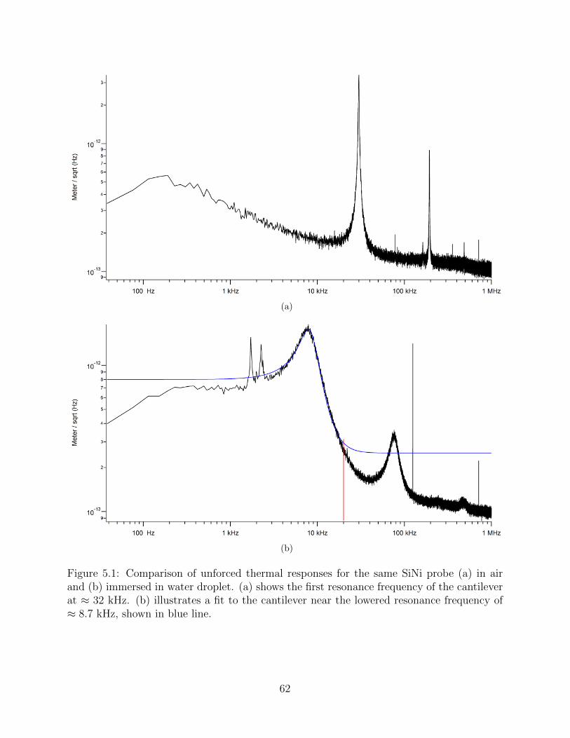
(a)
(b)
Figure 5.1: Comparison of unforced thermal responses for the same SiNi probe (a) in airand (b) immersed in water droplet. (a) shows the first resonance frequency of the cantileverat ≈ 32 kHz. (b) illustrates a fit to the cantilever near the lowered resonance frequency of≈ 8.7 kHz, shown in blue line.
62

(a)
(b)
Figure 5.2: Comparison of cantilever tune graphs with dither forcing for the same SiNiprobe. (a) The drive amplitude in Volts to achieve a target of 1 V in air was ≈ 850 mV.The fundamental resonant peak is distinctly captured as seen and the teal line illustratesthe phase. The vertical black line indicates the set drive frequency which is 95% of the firstmodal frequency in the tune displayed. (b) When the tip and holder are immersed in waterdroplet a forest of peaks appear due to resonant cavity effect. A drive amplitude of ≈ 1.98 Vwas required to achieve a target amplitude of 0.3 V at the chosen drive frequency. The plotin red is the thermal response of the cantilever, which helps choose the proper resonancepeak.
63
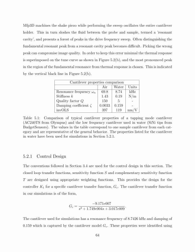
Mfp3D machines the shake piezo while performing the sweep oscillates the entire cantilever
holder. This in turn sloshes the fluid between the probe and sample, termed a ’resonant
cavity’, and presents a forest of peaks in the drive frequency sweep. Often distinguishing the
fundamental resonant peak from a resonant cavity peak becomes difficult. Picking the wrong
peak can compromise image quality. In order to keep this error minimal the thermal response
is superimposed on the tune curve as shown in Figure 5.2(b), and the most pronounced peak
in the region of the fundamental resonance from thermal response is chosen. This is indicated
by the vertical black line in Figure 5.2(b).
Cantilever properties comparisonAir Water Units
Resonance frequency ωn 69.8 8.74 kHzStiffness k 1.43 0.19 N/mQuality factor Q 150 5 -Damping coefficient ζ 0.0033 0.159 -invOLS 397 119 nm/V
Table 5.1: Comparison of typical cantilever properties of a tapping mode cantilever(AC240TS from Olympus) and the low frequency cantilever used in water (SiNi tips fromBudgetSensors). The values in the table correspond to one sample cantilever from each cat-egory and are representative of the general behavior. The properties listed for the cantileverin water have been used for simulations in Section 5.2.1.
5.2.1 Control Design
The conventions followed in Section 3.4 are used for the control design in this section. The
closed loop transfer functions, sensitivity function S and complementary sensitivity function
T are designed using appropriate weighting functions. This provides the design for the
controller K1 for a specific cantilever transfer function, Gc. The cantilever transfer function
in our simulations is of the form,
Gc =−9.171e007
s2 + 1.749e004s+ 3.017e009.
The cantilever used for simulations has a resonance frequency of 8.7426 kHz and damping of
0.159 which is captured by the cantilever model Gc. These properties were identified using
64
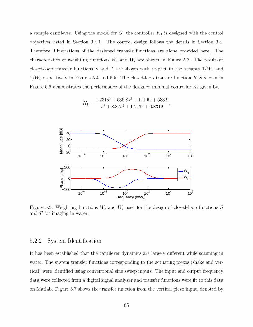
a sample cantilever. Using the model for Gc the controller K1 is designed with the control
objectives listed in Section 3.4.1. The control design follows the details in Section 3.4.
Therefore, illustrations of the designed transfer functions are alone provided here. The
characteristics of weighting functions Ws and Wt are shown in Figure 5.3. The resultant
closed-loop transfer functions S and T are shown with respect to the weights 1/Ws and
1/Wt respectively in Figures 5.4 and 5.5. The closed-loop transfer function K1S shown in
Figure 5.6 demonstrates the performance of the designed minimal controller K1 given by,
K1 =1.231s3 + 536.8s2 + 171.6s+ 533.9
s3 + 8.87s2 + 17.13s+ 0.8319.
10−4
10−2
100
102
104
106−20
0
20
40
Mag
nitu
de [d
B]
10−4
10−2
100
102
104
106−100
0
100
Pha
se [d
eg]
Frequency (w/wb)
Ws
Wt
Figure 5.3: Weighting functions Ws and Wt used for the design of closed-loop functions Sand T for imaging in water.
5.2.2 System Identification
It has been established that the cantilever dynamics are largely different while scanning in
water. The system transfer functions corresponding to the actuating piezos (shake and ver-
tical) were identified using conventional sine sweep inputs. The input and output frequency
data were collected from a digital signal analyzer and transfer functions were fit to this data
on Matlab. Figure 5.7 shows the transfer function from the vertical piezo input, denoted by
65

10−6
10−4
10−2
100
102
104
−40
−20
0
Mag
nitu
de [d
B]
10−6
10−4
10−2
100
102
104
0
50
100
Pha
se [d
eg]
Frequency (w/wb)
S1/W
s
Figure 5.4: Design of the sensitivity transfer function S with Gc transfer function for in-waterimaging.
10−6
10−4
10−2
100
102
104
−400
−200
0
Mag
nitu
de [d
B]
10−6
10−4
10−2
100
102
104−400
−200
0
Pha
se [d
eg]
Frequency (w/wb)
T1/W
t
Figure 5.5: Design of the complementary sensitivity transfer function T with Gc transferfunction for in-water imaging.
uz in Chapter 2, to the cantilever deflection signal ym collected by the photo-sensitive diode
sensor. The transfer function from the shake piezo input, denoted by ud, to the cantilever
deflection is shown in Figure 5.8. The data and the corresponding fit show that the dither
piezo is predominantly active only beyond a frequency of 3 kHz. Therefore, the control effort
cannot be directed entirely through the dither piezo. The following relation is used to design
66
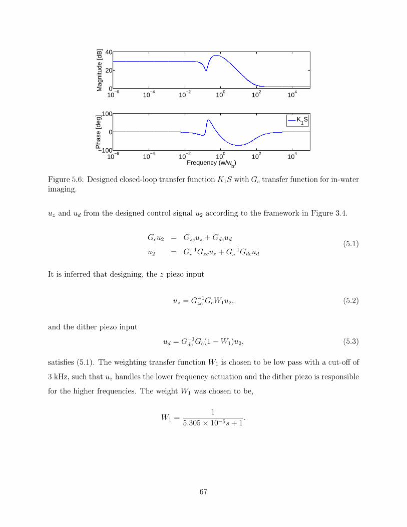
10−6
10−4
10−2
100
102
1040
20
40
Mag
nitu
de [d
B]
10−6
10−4
10−2
100
102
104−100
0
100
Pha
se [d
eg]
Frequency (w/wb)
K1S
Figure 5.6: Designed closed-loop transfer function K1S with Gc transfer function for in-waterimaging.
uz and ud from the designed control signal u2 according to the framework in Figure 3.4.
Gcu2 = Gzcuz +Gdcud
u2 = G−1c Gzcuz +G−1
c Gdcud(5.1)
It is inferred that designing, the z piezo input
uz = G−1zc GcW1u2, (5.2)
and the dither piezo input
ud = G−1dc Gc(1−W1)u2, (5.3)
satisfies (5.1). The weighting transfer function W1 is chosen to be low pass with a cut-off of
3 kHz, such that uz handles the lower frequency actuation and the dither piezo is responsible
for the higher frequencies. The weight W1 was chosen to be,
W1 =1
5.305× 10⁻⁵s+ 1.
67

100
101
102
103
104
−20
0
20
Mag
nitu
de (
dB)
100
101
102
103
104
0
200
400
Pha
se (
deg)
Freq (Hz)
DataFit
Figure 5.7: The transfer function, Gzc, identified between the z piezo input uz and cantileverdeflection y. The piezo was set at a DC offset of 70 V, the middle of its total range.A cantilever submerged in water with an effective resonance of 8.65 kHz was used in thisidentification experiment. The dotted black line is frequency response of the minimal transferfunction fit numerically to the identification data collected. It is important that we have agood fit in the lower frequencies where uz will take the maximum load of control.
100
101
102
103
104−80
−60
−40
−20
Mag
nitu
de (
dB)
100
101
102
103
104
−100
0
100
Pha
se (
deg)
Freq (Hz)
DataFit
Figure 5.8: The transfer function, Gdc, identified between the dither piezo input ud andcantilever deflection y. A cantilever submerged in water with an effective resonance of 8.65kHz was used in this identification experiment. The dotted black line is frequency responseof minimal transfer function fit numerically to the identification data collected.
The redefined controller is provided by the relation,
Q1 =
G−1zc GcW1K1
G−1dc Gc(1−W1)K1
, (5.4)
68

−200
0
200
To:
Out
(1)
−180
0
180
To:
Out
(1)
−200
0
200
To:
Out
(2)
101
102
103
104
105
106
107
108
109
−720
0
720
To:
Out
(2)
Frequency (rad/sec)
Mag
(dB
) ; P
hase
(de
g)
Figure 5.9: Frequency response of the transfer function Q1 in (5.4). Q1 is the system modelfrom em to uz (shown as Out(1)) and ud (shown as Out(2)).
which takes em the measured error between the cantilever deflection y and the reference tra-
jectory y and outputs the control inputs uz and ud for the two driving piezos. The frequency
response for Q1 is illustrated in Figure 5.9, where Out(1) denotes uz and Out(2) denotes
ud. It is necessary to note that there is no non-dimensionalization during implementation.
It was merely used as a technique to make the numerical computations and analysis more
convenient.
The identified transfer function Gz between z piezo input uz and output v is used to verify
the cantilever model by using G−1z Gzc. The frequency response of Gz identified is shown in
Figure 5.10.
5.2.3 Experiment Setup
An integrated Digital Signal Processing (DSP) board with on-board analog-digital (A/D)
and digital-analog (D/A) conversion interfaces was used. The model of the board used is
P25m from Innovative Integration that is mounted with a TI C6713 DSP chip. Figure 5.11
shows the experimental arrangement used with respect to the AFM.
69

100
101
102
103
104
−30
−20
−10
0
Mag
nitu
de (
dB)
100
101
102
103
104
−1000
100200300
Pha
se (
deg)
Freq (Hz)
DataFit
Figure 5.10: The transfer function, Gz, identified between the z piezo input uz and outputv. The piezo was set at a DC offset of 70 V, the middle of its total range. A digital signalanalyzer was used for system identification giving sine sweep inputs to the system. Theblack dotted line shows frequency response of numerical transfer function fit obtained.
Figure 5.11: Closed-loop experimental arrangement featuring the Digital Signal Processingboard complete with A/D and D/A components.
The sequence of the experiment is as follows. Upon identifying the cantilever transfer
function and engaging it onto the sample surface using proportional-integral control, the
raster scan in the lateral direction is begun. The cantilever deflection denoted by ym and the
sinusoidal signal g of the form g0 cosωt used to actuate the dither or shake piezo are drawn
from the AFM system to the DSP’s analog inputs. The DSP chip runs the controller dy-
namics as well as the mock system dynamics in tandem. Subsequently, the control inputs for
the z and dither piezo are computed and mapped to the D/A ports of the DSP board. Thus
70

the closed-loop operation is completed. The reference trajectory y generated by the mock
system dynamics on the DSP and the cantilever deflection signal from PSD are collected to
obtain the tracking error signal, which can then be used for disturbance/force estimation.
However, it must be noted that a very high sampling rate of closed loop operation is required
to robustly deduce the force and sample properties from the error data.
Figure 5.12: Comparison of cantilever deflection (y in blue) and reference trajectory (y inred) in current experimental set up at 40 kHz sampling. The poor sampling is evident fromthe y illustration.
With the current DSP hardware setup, the maximum achievable sampling rate was found
to be 40-45 kHz. As a consequence, for a cantilever resonance frequency in the range of ≈ 8.7
kHz only about four points are sampled every cycle of oscillation. Owing to the lacking in
hardware, it was not feasible to incorporate the modeled interaction force term d in the mock
system on the DSP module. The absence of d implies that the disturbance encountered in the
experiment is higher than what the controller was modeled for, i.e. the disturbance is now d
(tip-sample interaction force) in place of d−d. These factors result in a large initial mismatch
between the cantilever deflection y and the reference trajectory y. Furthermore, the resonant
cavity owing to oscillation of the cantilever holder in water induces uncertainties in the model.
Therefore, the regulation accomplished under available experimental conditions was not as
expected from the simulations (see Figure 5.12). However, higher scanning rates will resolve
most of these issues and is indispensable to effectively demonstrate this experiment.
71

5.3 Summary
Experimental validation with available hardware was not feasible for in-air imaging with
typical tapping mode cantilevers. Efforts to develop in-house FPGA-based hardware were
not successful. Therefore, a proof of concept experiment was designed where the imaging was
performed in water in order to reduce the natural frequency of the cantilever and thereby the
frequency of the signals to be handled by the controller. Redesign of control parameters, and
issues encountered in this experiment with the current DSP-based hardware arrangement
have been discussed along with the results achievable. Higher speed electronics will alleviate
most of the problems faced and facilitate imaging in air, which can prove the efficacy of the
designed controller better.
72

CHAPTER 6
CONCLUSION
6.1 Summary and Analysis
Atomic force microscopes are at the cutting edge of nanotechnology. However, considerable
challenges need to be met to realize their full potential. A major setback arises from the low
bandwidth of imaging in AFMs. In particular, it is a drawback while studying processes and
properties of biological specimens that have variations spatially and temporally. Work done
in order to address the problem of low bandwidth in the AFM community predominantly
comprises of hardware design and alterations with least emphasis on control-system tools.
This dissertation has devised a new dynamic mode for AFMs that will facilitate high-speed
imaging without the frills of major hardware fabrication. The mode makes extensive use of
system tools. The salient features of the proposed imaging mode are:
• The control design that drives the imaging is model-based and therefore makes use of
the system characteristics effectively.
• Amplitude modulation fails when the time scale separation between lateral positioning
bandwidth and cantilever resonance frequency varies only by a small factor. The “fast”
deflection signal of the cantilever is used instead of the traditionally used amplitude
signal for force regulation.
• The cantilever deflection is controlled to track a “deflection-like” signal produces by a
a fictitious system that is analogous to the cantilever dynamics, except it is assumed
that the sample input to the fictitious system is constant.
• The non-linearity in the system model coming from the tip-sample interaction force
73

is modeled as a disturbance enabling linear control design. Robust control design
for force regulation through disturbance rejection has been performed. Notably, the
regulation action does not affect the property estimates obtained through the imaging
mode since the estimation procedures make use of the error from tracking. Regulation
ensures that the tip stays close enough to the sample surface.
• The designs were all performed using the cantilever dynamic model Gc. It is important
to note that the control designs could have been done for the transfer function given
by[Gzc Gdc
]T.
• This enables consequent estimation of the disturbance through an appropriately de-
signed signal. Disturbance estimates translate to interaction force estimate, which is
the most informative/fundamental data that can be obtained from an imaging exper-
iment.
• The interaction forces are functions of tip-sample separation (which changes in the
presence of sample features) and its properties. Therefore, by suitably fitting models
to the force data, sample topography as well as physical properties such as elasticity,
hardness can be estimated and this has been demonstrated.
• Experimental validation of the new imaging mode by deploying it on a low resonance
frequency cantilever in the available commercial AFM system was carried out.
6.2 Future Research Directions
The following points outlines how the scope of this dissertation can be extended to future
work.
• Alternate approaches for control design such as nonlinear control design using Lya-
punov functions and use of S-procedure need to be further explored. These possible
approaches have been briefed in Appendix A and B.
74

• Considering the fact that existing dynamic modes of AFM operation use derivatives
of the deflection signal such as amplitude for regulation, the implementation hardware
in current modules have low sampling rates (10 − 100kHz). Whereas, the proposed
imaging mode effects force regulation using the fast deflection signal whose frequency
is in the order of 100− 300kHz. Validation experiments at proportionally scaled lower
frequencies could only be used to demonstrate force regulation owing to the limitations
of DSP operating bandwidths.
• The high frequency cantilever oscillation necessitates sampling rates of a few MHz (3-
10MHz). FPGA based boards that can take in and give out data over four channels
with a closed-loop frequency of a few MHz are available. Developing a FPGA based
hardware setup that can realize the required high closed-loop frequencies (in x and z
directions) is being pursued. While using actual tapping mode cantilevers and high
bandwidth computational power in the closed-loop video-rate imaging can be effected.
• Additionally, a high bandwidth nanopositioning system is required to demonstrate the
effects of our idea. The FPGA based hardware may be used to provide inputs to the
higher bandwidth lateral positioning system. The control designs demonstrated in [6]
can be used to obtain further lateral bandwidth improvements in conjunction with the
fast imaging.
• This dissertation has illustrated some ways to estimate sample properties from the force
estimate but these are not exhaustive. Characterization of relation between robustness
of estimates and force model employed should be explored.
75

APPENDIX A
ALTERNATE APPROACHES
A.1 BACKSTEPPING
In this section, cantilever model analogous to the one in Section 3.1 is considered for the
most part with certain modifications that are explained. Prior to using the disturbance
rejection approach, nonlinear control design considerations were made. These are briefed in
this section of the appendix.
Backstepping approach is commonly used to design stabilizing control for systems with
nonlinear dynamics. Equations of the form,
X = fx(X) + gx(X), ψ
ψ = fψ(X,ψ) + gψu1,(A.1)
constitute the structure of this approach. Here, X ∈ Rn, n ≥ 1, ψ is typically a scalar, u1 is
the scalar input to the system and the functions denoted by f ’s become zero at the origin.
In the first case, a control signal u2 in addition to vertical actuation v is considered. Based
on backstepping approach the vertical actuation signal v is modeled to be derived from a
dynamical system as explained in the following. This is done in order to pull v out of the
nonlinear function term F .
The cantilever dynamic equations are given by,
d2p
dt2+ 2ζωn
dp
dt+ ω2
np = ud +1
mF (p1 − h− v). (A.2)
Here, ud = bω2n cos(ωt) + bω2
nu2(t), i.e. in addition to the generic dither input bω2n cos(ωt),
we consider an additional input, bω2nu2(t).
76
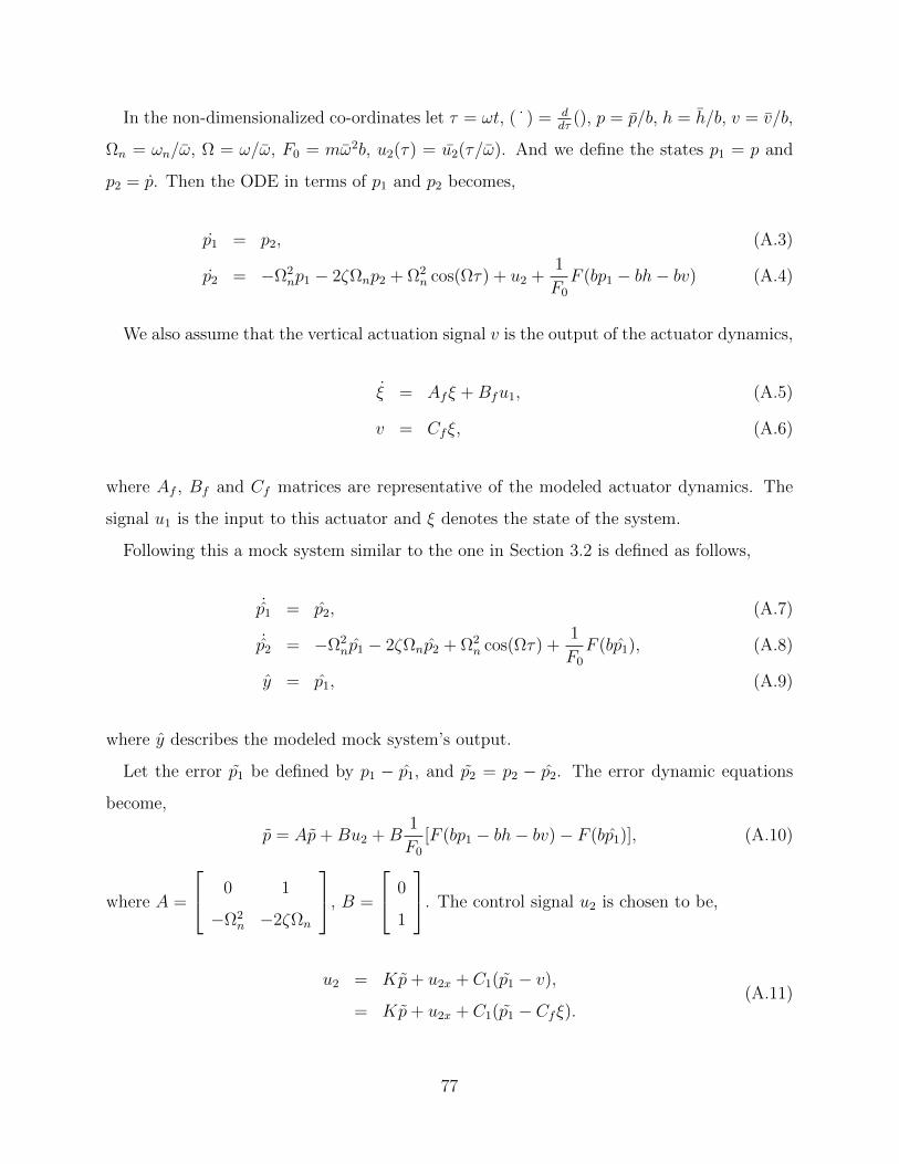
In the non-dimensionalized co-ordinates let τ = ωt, ( ˙ ) = ddτ
(), p = p/b, h = h/b, v = v/b,
Ωn = ωn/ω, Ω = ω/ω, F0 = mω2b, u2(τ) = u2(τ/ω). And we define the states p1 = p and
p2 = p. Then the ODE in terms of p1 and p2 becomes,
p1 = p2, (A.3)
p2 = −Ω2np1 − 2ζΩnp2 + Ω2
n cos(Ωτ) + u2 +1
F0
F (bp1 − bh− bv) (A.4)
We also assume that the vertical actuation signal v is the output of the actuator dynamics,
ξ = Afξ +Bfu1, (A.5)
v = Cfξ, (A.6)
where Af , Bf and Cf matrices are representative of the modeled actuator dynamics. The
signal u1 is the input to this actuator and ξ denotes the state of the system.
Following this a mock system similar to the one in Section 3.2 is defined as follows,
˙p1 = p2, (A.7)
˙p2 = −Ω2np1 − 2ζΩnp2 + Ω2
n cos(Ωτ) +1
F0
F (bp1), (A.8)
y = p1, (A.9)
where y describes the modeled mock system’s output.
Let the error p1 be defined by p1 − p1, and p2 = p2 − p2. The error dynamic equations
become,
p = Ap+Bu2 +B1
F0
[F (bp1 − bh− bv)− F (bp1)], (A.10)
where A =
0 1
−Ω2n −2ζΩn
, B =
0
1
. The control signal u2 is chosen to be,
u2 = Kp+ u2x + C1(p1 − v),
= Kp+ u2x + C1(p1 − Cfξ).(A.11)
77

Mean value theorem is applied to the force term F in the error dynamic equations (A.10) ,
˙p = Ap+BKp+Bu2x +BC1(p1 − v) +BΘ1
F0
(bp1 − bv − bh) (A.12)
= (A+BK)p+Bu2x +B(C1 + Θ1
F0
)(bp1 − bv)−Θ1
F0
Bbh. (A.13)
The term (A+BK)TP +P (A+BK) is assumed equal to −Q with Q > 0 by design. The
following Lyapunov energy function is chosen,
V (p) = pTP p (A.14)
where matrix P is positive-definite. The derivative of the energy function yields,
V = −pTQp+ 2pTPBu2x + 2pTPB(C1 +1
F0
Θ)[bp1 − bv −Θbh
C1 + Θ], (A.15)
where Θ = ∂f∂z
(z) and z lies in [bp1 − bv − bh, bp1]. The variables K, P , C1, v and u2x are
free to be designed. However, this approach not only calls for nonlinear control design but
imposes that a model of the interaction forces be known. The force model is required for
computation of the slope term Θ, which varies temporally.
Alternately, the following design could be considered,
p1 = p2, (A.16)
p2 = −Ω2np1 − 2ζΩnp2 + Ω2
n cos(Ωτ) +1
F0
Fts(bp1 − bCfξ), (A.17)
ξ = Afξ +Bf (h+ v), (A.18)
h+ v = Cfξ, (A.19)
where the inputs h and v are both modeled to be raw inputs of the filter ξ. Output of filter
represents the nature of sample profile signal in real samples. The state space vector x is
defined as [p1 p2 ξ]T . The complete system in terms of the state space co-ordinates is defined
by
78
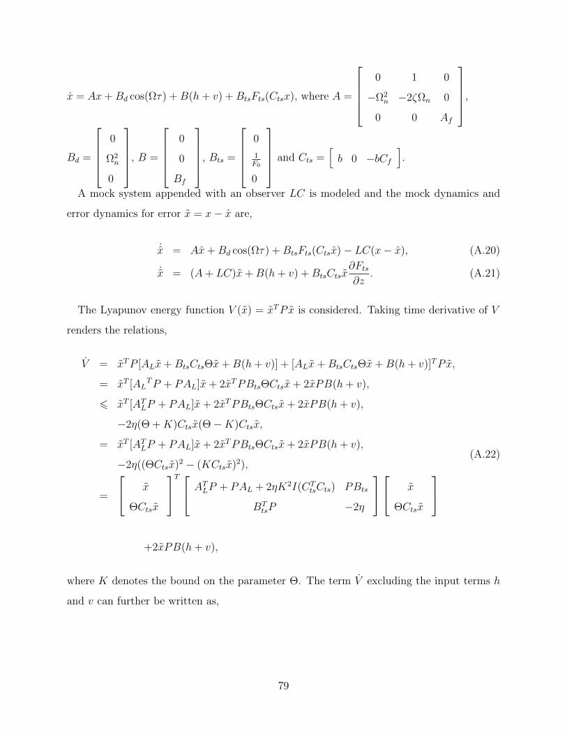
x = Ax+Bd cos(Ωτ) +B(h+ v) +BtsFts(Ctsx), where A =
0 1 0
−Ω2n −2ζΩn 0
0 0 Af
,
Bd =
0
Ω2n
0
, B =
0
0
Bf
, Bts =
0
1F0
0
and Cts =[b 0 −bCf
].
A mock system appended with an observer LC is modeled and the mock dynamics and
error dynamics for error x = x− x are,
˙x = Ax+Bd cos(Ωτ) +BtsFts(Ctsx)− LC(x− x), (A.20)
˙x = (A+ LC)x+B(h+ v) +BtsCtsx∂Fts∂z
. (A.21)
The Lyapunov energy function V (x) = xTPx is considered. Taking time derivative of V
renders the relations,
V = xTP [ALx+BtsCtsΘx+B(h+ v)] + [ALx+BtsCtsΘx+B(h+ v)]TPx,
= xT [ALTP + PAL]x+ 2xTPBtsΘCtsx+ 2xPB(h+ v),
6 xT [ATLP + PAL]x+ 2xTPBtsΘCtsx+ 2xPB(h+ v),
−2η(Θ +K)Ctsx(Θ−K)Ctsx,
= xT [ATLP + PAL]x+ 2xTPBtsΘCtsx+ 2xPB(h+ v),
−2η((ΘCtsx)2 − (KCtsx)2),
=
x
ΘCtsx
T ATLP + PAL + 2ηK2I(CTtsCts) PBts
BTtsP −2η
x
ΘCtsx
+2xPB(h+ v),
(A.22)
where K denotes the bound on the parameter Θ. The term V excluding the input terms h
and v can further be written as,
79

x
ΘCtsx1F0
T ATLP + PAL + 2ηK2CTtsCts PBts
BtsTP −2η
x
ΘCtsx1F0
.
The assumptions η = η 1F 20
, Bts =
0
1
0
, AL = A + LC are made. This set up although
linear in P and η posed difficulties because the sample profile h is unknown and requires to
be determined. Modeling the sample height input as a disturbance was considered before
establishing the design used in this dissertation where the tip-sample interaction force term
F is modeled as a disturbance enabling linear control design.
A.2 S-PROCEDURE
S-procedure is a technique used for problems with quadratic constraints. It has wide appli-
cations in controls, which is explained in great detail along with linear-matrix-inequalities
based solutions in book [42]. Firstly, the basics of S-procedure are introduced and then its
application to our problem of disturbance rejection is highlighted.
For functions F0 and F1 ∈ Rn×n such that F0 = F T0 , F1 = F T
1 , it is straightforward to
prove that ∀z,
zTF1z ≥ 0⇒ zTF0z ≥ 0.
It is true when ∃τ ∈ R, τ ≥ 0 and F0 ≥ τF1. The converse also holds when constraint
qualification, ∃ a point µ such that µTF1µ > 0 holds. This result is termed lossless S-
procedure. Proof of converse condition is not provided here.
Similarly, in case of strict inequalities if there exists τ ∈ R, τ ≥ 0 with F0 > τF1 then ∀z,
zTF1z ≥ 0, z 6= 0⇒ zTF0z > 0.
Again, the converse holds if ∃ a point µ such that µTF1µ > 0 holds.
Using error dynamic equations for p = p− p from (3.9) and assuming a Lyapunov function
80
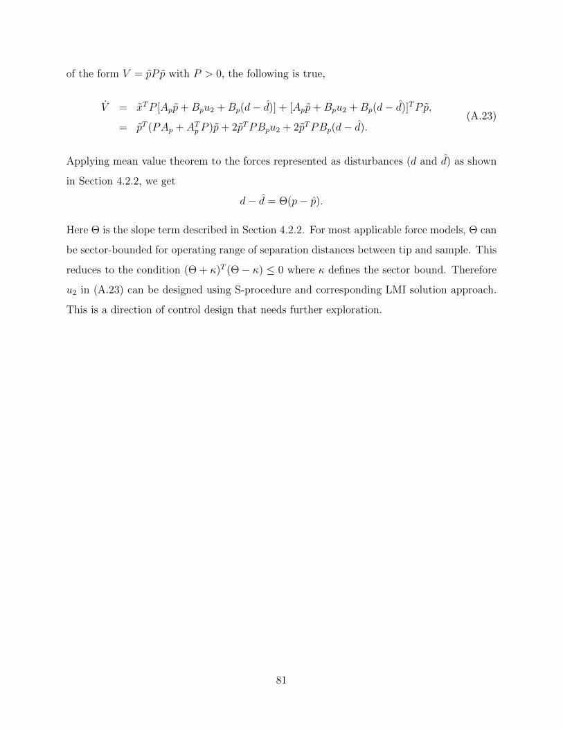
of the form V = pP p with P > 0, the following is true,
V = xTP [App+Bpu2 +Bp(d− d)] + [App+Bpu2 +Bp(d− d)]TP p,
= pT (PAp + ATp P )p+ 2pTPBpu2 + 2pTPBp(d− d).(A.23)
Applying mean value theorem to the forces represented as disturbances (d and d) as shown
in Section 4.2.2, we get
d− d = Θ(p− p).
Here Θ is the slope term described in Section 4.2.2. For most applicable force models, Θ can
be sector-bounded for operating range of separation distances between tip and sample. This
reduces to the condition (Θ + κ)T (Θ− κ) ≤ 0 where κ defines the sector bound. Therefore
u2 in (A.23) can be designed using S-procedure and corresponding LMI solution approach.
This is a direction of control design that needs further exploration.
81

APPENDIX B
AVERAGING METHODS FOR AMPLITUDEDYNAMICS
Sample profile measurement in an atomic force microscope is done using either the contact
mode or the tapping mode. We have considered the constant amplitude or tapping mode
measurement technique for our purposes. The amplitude of oscillation changes everytime
the cantilever comes across a feature on the sample. The constant amplitude mode of
operation aims at maintaining this amplitude of oscillation constant, and the displacement
effort required to achieve this gives a measure of the features on the sample.
B.1 Using Lagrangian equations for A, φ dynamics
In averaging methods like KBM the input h(t) is assumed to be constant and therefore these
methods are reliable only for h(t) up to a frequency of 2KHz. Assuming that the solution of
the non-linearly perturbed system will be of the form p(t) = a cos(ωt + φ), the Lagrangian
dynamics procedure was followed to derive the second order dynamic equations in a and φ.
B.1.1 Second order equations
a1 = a
a1 = a2
a2 = a1ω2 + 2a1ωφ2 + a1φ
22 − a1ω
2n + ω2
nb cos(φ1)− 2ζωna2
+1
πm
∫ 2π
0
F (a1 sin(θ)− h− v) sin(θ)dθ
82
φ1 = φ
φ1 = φ2
φ2 = −2a2
a1
ω − 2a2
a1
φ2 −ω2nb sin(φ)
a1
− 2ζωn(ω + φ2)
In the above equations, θ = ωt+ φ1.
B.1.2 Reduced - first order
The equations in the previous section have been reduced to the following form after elim-
inating the second order terms. These under some additional constraints are similar to
KBM.
2aωφ = −aω2 + aω2n − ω2
nb cos(φ) + 2ζωna−1
πm
∫ 2π
0
F (a1 sin(θ)− h− v) sin(θ)dθ
a(2ω
a) = −ω
2nb sin(φ)
a− 2ζωn(ω + φ)
At higher frequencies, this model like the KBM model does not remain valid, that is it
does not approximate the cantilever deflection dynamics well.
83

REFERENCES
[1] G. Binnig, C.F.Quate, and C. Gerber, “Atomic force microscope,” Physical ReviewLetters, vol. 56, no. 9, pp. 930–933, March 1986.
[2] S. Gould, O. Marti, B. Drake, L. Hellemans, C. E. Bracker, H. PK., N. L. Keder, M. M.Eddy, and G. D. Stucky, “Molecular resolution images of amino acid crystals with theatomic force microscope,” Nature, vol. 332, no. 22, pp. 332–334, March 1988.
[3] B. Drake, C. Prater, A. Weisenhorn, S. Gould, T. Albrecht, C. Quate, D. Cannell,H. Hansma, and P. Hansma, “Imaging crystals, polymers, and processes in water withthe atomic force microscope,” Science, vol. 243, no. 4898, pp. 1586–1589, March 1989.
[4] R. Garcia and R. Perez, “Dynamic atomic force microscopy methods,” Surf. Sci. Rep.,vol. 47, p. 197, 2002.
[5] F. Giessibl, S. Hembacher, H. Bielefeldt, and J. Mannhart, “Subatomic features on thesilicon (111)-(77) surface observed by atomic force microscopy,” Science, vol. 289, no.5478, pp. 422–425, July 2000.
[6] C. Lee and S. Salapaka, “Fast robust nanopositioning - a linear-matrix-inequalities-based optimal control approach,” IEEE/ASME Transactions on Mechatronics, vol. 14,no. 4, pp. 414–422, August 2009.
[7] S. Salapaka, T. De, and A. Sebastian, “A robust control based solution to the sample-profile estimation problem in fast atomic force microscopy,” International Journal ofRobust and Nonlinear Control, vol. 15, pp. 821–837, 2005.
[8] G. Fantner, G. Schitter, and et. al. J.H. Kindt, “Components for high speed atomicforce microscopy,” Ultramicroscopy, vol. 106, no. 8, pp. 881–887, 2006.
[9] K. Leang and A. Fleming, “High speed afm scanner: Design and drive considerations,”in American Control Conference, 2008, pp. 3188–3193.
[10] S. Polit and J. Dong, “Design of high-bandwidth high-precision flexure-based nano-positioning modules,” Journal of Manufacturing Systems, 2010.
[11] D. A.Walters, J. P. Cleveland, N. H. Thomson, P. K. Hansma, M. A. Wendman, G. Gur-ley, and V. V. Elings, “Short cantilevers for atomic force microscopy,” Review of Scien-tific Instruments, vol. 67, pp. 3583 – 3590, Oct 1996.
84

[12] M. Kitazawa, K. Shiotani, and A. Toda1, “Batch fabrication of sharpened silicon nitridetips,” Japanese Journal of Applied Physics, vol. 42, pp. 4844–4847, 2003.
[13] T. Ando, “High-speed atomic force microscopy coming of age,” Nanotechnology, vol. 23,p. 27, January 2012.
[14] T. Sulchek, S. C. Minne, J. D. Adams, D. A. Fletcher, A. Atalar, C. F. Quate, andD. M. Adderton, “Dual integrated actuators for extended range high speed atomic forcemicroscopy,” Applied Physics Letters, vol. 75, no. 11, p. 1637, July 1999.
[15] T. Ando, N. Kodera, E. Takai, D. Maruyama, K. Saito, and A. Toda, “A high-speedatomic force microscope for studying biological macromolecules,” Proceedings of theNational Academy of Sciences, vol. 98, no. 22, p. 034106, 2001.
[16] T. Ando, T. Uchihashia, and T. Fukumac, “High-speed atomic force microscopy fornano-visualization of dynamic biomolecular processes,” Progress in Surface Science,vol. 83, no. 7-9, pp. 337–437, November 2008.
[17] L. M. P. et al, “Breaking the speed limit with atomic force microscopy,” Nanotechnology,vol. 18, no. 4, 2007.
[18] M. H. Despont, U. Drechsler, U. T. Durig, W. Haberle, M. I. Lutwyche, H. E. Rothuizen,R. Stutz, R. Widmer, and G. K. Binnig, “The “millipede”—more than thousand tipsfor future afm storage,” IBM Journal of Research and Development, vol. 44, no. 3, pp.323–340, May 2000.
[19] S. Salapaka, A. Sebastian, J. P. Cleveland, and M. V. Salapaka., “High bandwidthnano-positioner: A robust control approach,” IEEE Transactions on Control SystemsTechnology, vol. 73, pp. 3232–3241, March 2002.
[20] G. Schitter, F. Allgower, and A. Stemmer, “A new control strategy for high-speedatomic force microscopy,” Nanotechnology, vol. 15, no. 1, 2004.
[21] S. Salapaka, T. De, and A. Sebastian, “Sample-profile estimate for fast atomic forcemicroscopy,” Applied Physics Letters, vol. 87, no. 5, 2005.
[22] C. Lee and S. Salapaka, “Fast imaging with alternative signal for dynamic atomic forcemicroscopy,” Applied Physics Letters, vol. 97, no. 13, 2010.
[23] D. Sahoo, A. Sebastian, and M. V. Salapaka, “Transient-signal-based sample-detectionin atomic force microscopy,” Applied Physics Letters, vol. 83, no. 26, pp. 5521–5523,December 2003.
[24] D. Sahoo, A. Sebastian, and M. V. Salapaka, “Harnessing the transient signals in atomicforce microscopy,” International Jorunal of Robust and Nonlinear Control, vol. 15, pp.805–820, 2005.
85
[25] D. Sahoo, P. Agarwal, and M. V. Salapaka, “Transient force atomic force microscopy:A new nano-interrogation method,” in American Control Conference, 2007, pp. 2136–2140.
[26] G. Schitter, “Field programmable analog array (fpaa) based control of an atomic forcemicroscope,” in Proceedings of American Control Conference, June 2008, pp. 2690 –2695.
[27] K. Johnson, K. Kendall, and A. Roberts, “Surface energy and the contact of elasticsolids,” Proceedings of the Royal Society, Lond.A, vol. 324, no. 1558, pp. 301–313,September 1971.
[28] B. Derjaguin, V. Muller, and Y. Toropov, “Effect of contact deformations on the adhe-sion of particles,” Journal of Colloid and Interface Science, vol. 53, no. 2, pp. 314–326,November 1975.
[29] H. Pollock, D. Maugis, and M. Barquins, “The force of adhesion between solid surfacesin contact,” Applied Physics Letters, vol. 33, no. 9, pp. 798–799, November 1978.
[30] K. Zhou, J.Doyle, and K. Glover, Robust and Optimal Control. Prentice Hall, UpperSaddle River, NJ 07458, 1996.
[31] C. Scherer, P. Gahinet, and M. Chilali, “Multiobjective output-feedback control via lmioptimization,” Automatic Control, IEEE Transactions on, vol. 42, no. 7, pp. 896–911,July 1997.
[32] G. Dullerud and F. Paganini, A Course in Robust Control Theory: A Convex Approach.Springer-Verlag, 2000.
[33] R. Garcia and A. S. Paulo, “Attractive and repulsive tip sample interaction regimes intapping mode atomic force microscopy,” Phys. Rev. B, vol. 60, no. 7, pp. 4961–4967,August 1999.
[34] G. Mohan, C. Lee, and S. Salapaka, “Control techniques for high-speed dynamic modeimaging in atomic force microscopes,” in Proceedings of the 50th IEEE Conference onDecision and Control and European Control Conference, CDC-ECC 2011, Orlando, FL,USA, 2011, pp. 651–656.
[35] J. Doyle, B. Francis, and A. Tannenbaum, Feedback Control Theory. New York:MacMillan, 1992.
[36] P. Maivald, H. Butt, S. Gould, C. B. Prater, B. Drake, J. Gurley, V. Elings, andP. Hansma, “Using force modulation to image surface elasticities with the atomic forcemicroscope,” Nanotechnology, vol. 2, pp. 103–106, February 1991.
[37] M. Stark, R. Guckenberger, A. Stemmer, and R. Stark, “Estimating the transfer func-tion of the cantilever in atomic force microscopy: A system indentification approach,”Journal of Applied Physics, vol. 98, pp. 114 904–114 904–7, December 2005.
86
[38] F. Giessibl, “A direct method to calculate tip-sample forces from frequency shifts infrequency-modulation atomic force microscopy,” Applied Physics Letters, vol. 78, no. 1,January 2001.
[39] P. A. Yuya, D. C. Hurley, and J. A. Turner, “Contact-resonance atomic force microscopyfor viscoelasticity,” Journal of Applied Physics, vol. 104, no. 7, pp. 074 916–074 916–7,June 2009.
[40] P. Agarwal and M. V. Salapaka, “Real time estimation of equivalent cantilever param-eters in tapping mode atomic force microscopy,” Applied Physics Letters, vol. 95, no. 8,pp. 083 113–083 113–3, September 2009.
[41] J. Sader, “Frequency response of cantilever beams immersed in viscous fluids withapplication to the atomic force microscope,” Journal of Applied Physics, vol. 84, no. 1,pp. 64–76, 1998.
[42] S. Boyd, L. E. Ghaoui, E. Feron, and V. Balakrishnan, Linear Matrix Inequalities inSystem and Control Theory. SIAM Studies in Applied Mathematics, 1994.
87


