30
c 2019 Yu Zhang

c© 2019 Yu Zhang

CLASSIFYING GITHUB REPOSITORIES WITH MINIMAL HUMAN EFFORTS
BY
YU ZHANG
THESIS
Submitted in partial fulfillment of the requirementsfor the degree of Master of Science in Computer Science
in the Graduate College of theUniversity of Illinois at Urbana-Champaign, 2019
Urbana, Illinois
Adviser:
Professor Jiawei Han

ABSTRACT
GitHub is a great platform for sharing software code, data, and other resources. To
improve search and analysis of a vast spectrum of resources on GitHub, it is necessary
to conduct automatic, flexible and user-guided classification of GitHub repositories. In
this paper, we study how to build a customized repository classifier with minimal human
annotation. Previous document classification methods cannot be directly applied to our task
due to three unique challenges: (1) multi-modal signals: besides text, signals in other
formats need to be explored to uncover the topic of a repository; (2) low data quality:
GitHub README files, usually containing code and commands, are noisier than typical text
data such as scientific papers and news; and (3) limited ground-truth: users cannot afford
to label many repositories for training a good classifier. To deal with the challenges above,
we propose GitClass, a framework to classify GitHub repositories under weak supervision.
Three key modules, heterogeneous network construction and embedding, keyword extraction
and topic modeling, as well as pseudo document generation, are used to tackle the above
three challenges, respectively. We conduct extensive experiments on three large-scale GitHub
repository datasets and observe evident performance boost over state-of-the-art embedding
and classification algorithms.
ii

To my parents, for their love and support.
iii

ACKNOWLEDGMENTS
I would firstly like to thank my advisor Professor Jiawei Han of the Department of Com-
puter Science at University of Illinois at Urbana-Champaign. He has provided me extensive
advice and suggestions not only on this thesis project, but also throughout my whole mas-
ter’s study. Under Professor Han’s guidance, my research skills have been greatly improved.
More importantly, his encouragement and support helped spark my interest in research, so
that I become determined to continue my research career by pursuing a Ph.D. degree.
Also, I would like to thank all of my research collaborators. It has been my great fortune
to join the Data Mining Research Group and get the chance to work with such a brilliant
group of peer researchers. From them, I have learned a lot, including how to formulate a
research problem, how to solve a problem, and how to write a research paper. In particular,
I would like to thank Xuan Wang, Professor Xiang Ren, and soon-to-be Professor Qi Li for
their valuable help in this thesis study.
iv

TABLE OF CONTENTS
CHAPTER 1 INTRODUCTION . . . . . . . . . . . . . . . . . . . . . . . . . . . . 1
CHAPTER 2 PRELIMINARIES . . . . . . . . . . . . . . . . . . . . . . . . . . . . 32.1 GitHub Repositories . . . . . . . . . . . . . . . . . . . . . . . . . . . . . . . 32.2 Heterogeneous Information Networks . . . . . . . . . . . . . . . . . . . . . . 4
CHAPTER 3 METHOD . . . . . . . . . . . . . . . . . . . . . . . . . . . . . . . . . 53.1 Overview . . . . . . . . . . . . . . . . . . . . . . . . . . . . . . . . . . . . . . 53.2 HIN Construction and Embedding . . . . . . . . . . . . . . . . . . . . . . . . 53.3 Keyword Extraction and Topic Modeling . . . . . . . . . . . . . . . . . . . . 83.4 Pseudo Document Generation and Neural Model Training . . . . . . . . . . 10
CHAPTER 4 EXPERIMENTS . . . . . . . . . . . . . . . . . . . . . . . . . . . . . 124.1 Experimental Setup . . . . . . . . . . . . . . . . . . . . . . . . . . . . . . . . 124.2 Does GitClass Achieve Supreme Performances? . . . . . . . . . . . . . . . . 144.3 How Does HIN Contribute to the Performances? . . . . . . . . . . . . . . . . 144.4 How Does Keyword Extraction Contribute to the Performances? . . . . . . . 164.5 How Do Pseudo Documents Contribute to the Performances? . . . . . . . . . 17
CHAPTER 5 RELATED WORK . . . . . . . . . . . . . . . . . . . . . . . . . . . . 20
CHAPTER 6 CONCLUSIONS AND FUTURE WORK . . . . . . . . . . . . . . . . 21
REFERENCES . . . . . . . . . . . . . . . . . . . . . . . . . . . . . . . . . . . . . . . 22
v

CHAPTER 1: INTRODUCTION
The computer science field embraces a culture of sharing source code and data, which
promotes active scientific exchange and rapid technological progress. As a web-based hosting
service for version control, GitHub has become a tremendously popular platform for code
and dataset sharing, with more than 96 million repositories and 31 million users in 20181.
With such a vast spectrum of software tools on GitHub, there is an urgent need of cat-
egorizing GitHub-based repositories to facilitate flexible search and analysis. GitHub has
proposed to use topic labels2 to represent a particular subject area. However, this practice
still encounters the following challenges: (1) Sparse annotations : GitHub requires contrib-
utors to provide topic tags for their repositories, which is often ignored. We checked one
dataset (Bioinformatics) used in our experiments, finding that 84% of the repositories have
no such tags. Whether a repository is tagged will substantially affect its ranking in searching
results. For example, when searching “phylogenetics” on GitHub, one repository phyx 3 with
the tag “phylogenetics” ranks the 6th, but another repository opentree4, with more stars
and forks but without the tag does not show up in the first 10 pages. In our experiment, we
successfully classify opentree into the Phylogenetics category, which may increase its chance
to be ranked higher. (2) Evolving label space: New topics are emerging and the label space is
evolving. For example, several repositories related to Generative Adversarial Nets were re-
leased soon after the publication of the NIPS 2014 paper5. However, “gan” had not become
a GitHub topic tag until 2017. (3) User-specific criteria: Different users may want to view
the repositories from different angles (e.g., some may care more on methodology, such as
“classification” vs. “clustering” whereas others on applications, such as ‘network-mining”
vs. “text-mining”).
The aforementioned problems indicate the demand of an automatic, flexible and user-
guided repository classification algorithm, where users specify the categories, and we build a
classifier to put repositories into the categories. However, it is too costly for users to annotate
a large set of repositories for training. To alleviate users’ effort, we define a weakly-supervised
repository classification task:
Definition 1.1 (Problem Definition) Given a set of unlabeled GitHub repositories, users
define the categories by providing a very small number of (in this paper, 10) repositories for
1https://octoverse.github.com/2https://help.github.com/en/articles/about-topics3https://github.com/FePhyFoFum/phyx4https://github.com/OpenTreeOfLife/opentree5https://github.com/topics/gan?o=asc&s=updated
1

each category, and our task is to assign appropriate category labels to other repositories.
In contrast with the well-studied document classification problem [10, 25, 30], our task
has three unique challenges:
Multi-modal signals: On GitHub, topics are often indicated by multi-modal information
(e.g., users) besides text (e.g., README files). How to jointly leverage such heterogeneous
signals in a coherent and principled way?
Low data quality: Noises are ubiquitous in text, and GitHub README files are even
more cluttered than other kinds of text (e.g., scientific papers and news), filled with topic-
irrelevant details such as code and commands. How to make our framework robust towards
severe noises?
Limited ground-truth: A small set of labeled repositories is insufficient to train a good
classifier. How to prevent the learned classifier from overfitting?
In this paper, we present a new GitClass framework that automatically classifies GitHub
repositories with minimal human efforts. Three key modules are proposed to solve the three
challenges mentioned above, respectively.
1. To deal with multi-modal signals, we propose to use heterogeneous information net-
works [22] to encode various relationships between words, repositories, users and pro-
vided labels.
2. To tackle low data quality, we introduce a keyword extraction and topic modeling
module. The keyword extraction step essentially serves as a noise filter. Given a set
of keywords, we learn a word distribution for each category through topic modeling.
3. To overcome the scarcity of ground-truth, we present a pseudo-document generation
technique [13], which leverages learned distributions to generate synthesized training
data.
We demonstrate the effectiveness of GitClass through extensive experiments on three
large-scale GitHub repository datasets. GitClass consistently outperforms the benchmark
embedding and classification techniques [14, 10, 25, 30, 18, 4, 13] by a large margin. More-
over, we validate the design of our framework by showing the positive contribution of each
module.
2

CHAPTER 2: PRELIMINARIES
2.1 GITHUB REPOSITORIES
Fig. 2.1 shows a sample GitHub repository1 associated with an influential graph embed-
ding paper [26]. With the help of GitHub API2, we are able to extract various information in
a repository, such as metadata, source code and team dynamics. In GitClass, the following
information will be exploited.
User Repository
Description
README Description
Figure 2.1: A sample GitHub repository [26] with user’s name, the repository name, descrip-tion and README (only the first paragraph is shown).
User. If two repositories share the same user (“tangjianpku” in Fig. 2.1), they are more
likely to have similar topics (e.g., machine learning).
Description. The description is a concise summary of the repository. It usually contains
topic-indicating keywords (e.g., “embedding” in Fig. 2.1).
README. The README file serves as the main text information in a repository. In
contrast to the description, it has a more detailed explanation of both topics and other issues
(e.g., installation processes, code usages, etc.). The latter part makes the text information
noisy and sparse in topic inference.
1https://github.com/tangjianpku/LINE2https://developer.github.com/v3/
3

We concatenate repository description and README into a single “document”, which
serves as the textual feature of a repository.
2.2 HETEROGENEOUS INFORMATION NETWORKS
Due to its power of accommodating multi-typed interconnected data [23, 22], heterogeneous
information network (HIN) is leveraged to integrate structured information (i.e., users) and
textual features in GitClass.
Heterogeneous Information Network. An HIN is defined as a graph G = (V , E) with a
node type mapping φ : V → TV and an edge type mapping ψ : E → TE . Either the number
of node types |TV | or the number of relation types |TE | is larger than 1.
Meta-Path. As we all know, one advantage of networks is the ability to go beyond direct
links and model higher-order relationships between nodes. In an HIN, meta-paths [23] are
proposed to describe long relationships by concatenating edge types. For an HIN G = (V , E),
a meta-path is a sequence of node/edge types M = V1-V2-...-VL (Vi ∈ TV and Vi-Vi+1 ∈ TEfor any i).
4

CHAPTER 3: METHOD
3.1 OVERVIEW
We lay out our GitClass framework in Fig. 3.1. GitClass consists of three key modules,
which are proposed to solve the three challenges mentioned in Introduction, respectively.
To deal with multi-modal signals, we propose an HIN construction and embedding module
(Section 3.2). Given a small set of user-labeled repositories, we first construct an HIN to
describe different kinds of connections between words, repositories, labels and users. Then
we adopt ESim [18], a meta-path guided heterogeneous network embedding technique, to
obtain good node representations.
To tackle low data quality, we introduce a keyword extraction and topic modeling mod-
ule (Section 3.3). For each user-specified category, we first extract keywords from labeled
repositories. This step essentially serves as a noise filter. Putting keywords and embedding
vectors together, we are able to learn a word distribution for each category through topic
modeling.
To overcome the scarcity of ground-truth, we present a pseudo-document generation tech-
nique (Section 3.4), where we create a large set of “pseudo training repositories” by sampling
words from the learned distributions. The synthesized documents, along with the original
training data, are fed into a convolutional neural network. Intuitively, the neural classifier
is fitting the learned word distributions instead of the small set of user guidance, which can
effectively prevent it from overfitting.
3.2 HIN CONSTRUCTION AND EMBEDDING
In HIN construction, four types of nodes are included: words (W ), repositories (R), labels
(L) and users (U). Since the goal of this module is to learn accurate word representations for
the subsequent topic modeling and classification steps, we adopt a word-centric star schema
[24, 25], which is shown in Fig. 3.2.
The constructed HIN considers four types of word co-occurrences:
(1) W–W . The word-word relations capture word co-occurrence information in local
contexts. Each time two words co-occur in the context of a given window size, there will be
one edge between them.
(2) W–R. The word-repository edges describe document-level co-occurrences, where the
edge weight between word wi and repository rj indicates the number of times wi appears in
5

User Guidance
MachineLearning
ComputerVision
NaturalLang. Proc.
HIN Construction and Embedding
word
repo
user
label
Keyword Extraction and Topic Modeling
MachineLearningbayesiangaussian
icml…
ComputerVisionvision
inceptionrcnn
…
NaturalLang. Proc.
seq2seqencoderlexicon
…
… ……
word 1word 2word 3repo 1user 1
Pseudo Doc Generationand Neural Net Training
Classification
MachineLearning
ComputerVision
NaturalLang. Proc.
MachineLearning
ComputerVision
NaturalLang. Proc.
Figure 3.1: The GitClass framework. Three key modules (i.e., HIN construction and em-bedding, keyword extraction and topic modeling, and pseudo document generation) are usedto tackle the aforementioned three challenges, respectively.
rj (i.e., term frequency, or tf(wi, rj)). From the perspective of second-order proximity [26],
W–R edges essentially model the fact that two words tend to have similar semantics when
they appear in the same repository.
(3) W–L. The word-label relations encode category-level word co-occurrences. The edge
weight between word wi and label lj is∑k: repository rk has label lj
tf(wi, rk). (3.1)
(4) W–U . The word-user relations capture user-level word co-occurrences. The edge
weight between word wi and user uj is∑k: repository rk belongs to user uj
tf(wi, rk). (3.2)
To encode multi-relational links into our node representations, we propose to use ESim
[18] as our HIN embedding algorithm. (There are several other choices, such as PTE [25]
and metapath2vec [4]. In our experiments, adopting ESim achieves the best performances.)
Intuitively, homogeneous node embedding methods [15, 6] rely on random walks to generate
node sequences and then maximize the likelihood of observing those sequences. ESim follows
the same idea, but the random walks are under the guidance of meta-paths. In GitClass,
we choose W–W , W–R–W , W–L–W and W–U–W as our meta-paths, where W–W reflects
first-order proximity between two words, and the other three denote different kinds of second-
order proximity.
Following the selected meta-paths, we can sample a large number of meta-path instances
6

seq2seq
icml
gaussian
cifar
rcnnvision
decoder
lexicon
icmlgaussianvision
seq2seq
rcnn…
repository1repository2repository3…
icmlgaussianvision
seq2seq
rcnn…
label1label2label3…
icmlgaussianvision
seq2seq
rcnn…
user1user2user3…
Figure 3.2: Our HIN can be decomposed into four networks all related to words. The W -Wnetwork describes first-order proximity between words. The W -R, W -L and W -U bipartitenetworks characterize three kinds of second-order proximity between words.
in our HIN (e.g., W–R–W is a valid node sequence, while W–W–R is not). Given a meta-
path M and its corresponding node sequence P = u1–u2–...–uL, the likelihood is defined
as
Pr(P|M) = Pr(u1|M)L−1∏i=1
Pr(ui+1|ui,M), (3.3)
where
Pr(v|u,M) =exp(f(u, v,M))∑v′∈V exp(f(u, v,M))
, (3.4)
and
f(u, v,M) = µM + pTMeu + qTMev + eTu ev. (3.5)
Here, µM is the global bias of meta-pathM. pM and qM are d-dimensional local bias ofM.
eu and ev are d-dimensional embedding vectors of nodes u and v, respectively.
For Pr(u1|M), we make it proportional to ∆1(u1|M)γ, where ∆i(u|M) represents the
number of path instances following M with the i-th node being u. This number can be
computed using dynamic programming [18]. γ is a widely used parameter to control the
effect of overly-popular nodes, which is set to 0.75 in previous work [14].
eu, ev, pM, qM and µM can be learned through maximizing the likelihood. In practice,
In practice, to accelerate the training process, negative sampling [14] is used to derive the
following loss function:
LM =∑
P followingM
log(σ(L−1∑i=1
f(ui, ui+1, ri)))+K∑k=1
EPk∼Pr−(P|M) log(1−σ(L−1∑i=1
f(uki , uki+1, ri))),
(3.6)
where Pk = uk1-uk2-...-ukL is sampled from a noise distribution Pr−(P|M) ∝∏L
i=1 ∆i(ui|M)γ,
and σ(·) is the sigmoid function.
7

3.3 KEYWORD EXTRACTION AND TOPIC MODELING
We now present our keyword selection step, which extracts strong topic indicators from
the noisy text data.
Suppose the user-labeled repositories can be represented as C sets R1, ...,RC , where C is
the number of classes andRi = {ri1, ..., riD} is the set of repositories with label li (1 ≤ i ≤ C).
(For simplicity of notation, we assume each class has the same number of (i.e., D) labeled
repositories here.) Intuitively, we need to consider the following two principles when selecting
representative terms in Ri.
Relevance. A representative term w should be relevant to Ri.
Distinctiveness. A representative term w should be much more relevant to Ri than it is
to Rj (j 6= i).
To composite the two factors above, we define the representativeness of term w in Ri as
r(w,Ri) =exp(tfidf(w,Ri))∑Cj=1 exp(tfidf(w,Rj))
, (3.7)
where tfidf(w,Ri) is the TFIDF score. Here the term frequency is the number of times w
appears in Ri (i.e.,∑D
d=1 tf(w, rid)), and the document frequency refers to the number of
labeled repositories containing w (i.e., |{rcd|w ∈ rcd, 1 ≤ c ≤ C, 1 ≤ d ≤ D}|). For each class
i (1 ≤ i ≤ C), we select T terms with the highest representativeness scores. These terms
are assumed to have a high relevance to Ri and low relevances to Rj (j 6= i).
Now we proceed to the topic modeling step. In the previous HIN embedding module, we
already have the embedding vector ew for each selected keyword w. We normalize it onto
a unit sphere (i.e., ew ← ew/||ew||). Given the keyword embeddings, we adopt von-Mises
Fisher (vMF) distributions [5, 13] to characterize word distributions for each category. To
be specific, the probability to generate keyword w from category i is defined as
f(w|li) = f(ew|µi, κi) = cp(κi) exp(κiµTi ew), (3.8)
where cp(κi) is a normalization constant. The vMF distribution can be interpreted as a
normal distribution on a unit sphere. There are two parameters: the mean direction vector
µi and the concentration parameter κi. The keyword embeddings concentrate around µi,
and are more concentrated if κi is large.
Given the extracted keywords, we can derive µi and κi using maximum likelihood esti-
mation [5]. The obtained semantic distribution f(·|µ̂i, κ̂i) can be viewed as a “cleaned” and
“smoothed” version of the noisy and small-sized user-annotated repositories.
8

Let us go back to the keyword selection step. One may ask why we define representative-
ness as the form in Eqn. (3.7). We now give a probabilistic explanation from the perspective
of vMF distributions.
We use a CD-dimension vector to represent each category li and each word w. One
dimension describes one user-labeled repositories r. (We have C ×D labeled repositories in
total.) For category i, its corresponding vector λi is defined as
λir =
1, repository r has label li
0. otherwise(3.9)
For each word w, its corresponding vector εw is defined as
εwr = tf(w, r) · idf(w,Ri), (3.10)
where Ri is the repository set containing r. Given the definition, we have
tfidf(w,Ri) = tf(w,Ri) · idf(w,Ri) =∑r∈Ri
tf(w, r) · idf(w,Ri) = λTi εw. (3.11)
Assume w is generated from a vMF distribution (then its corresponding vector should be
normalized onto a sphere, which is εw/||εw||), where µi = λi/||λi|| and κi = ||λi|| · ||εw|| =√D||εw|| (∀1 ≤ i ≤ C). In this way,
Pr(li|w) =f(w|li) Pr(li)∑Cj=1 f(w|lj) Pr(lj)
=cp(κi) exp(κiµ
Ti εw/||εw||) Pr(li)∑C
j=1 cp(κj) exp(κjµTj εw/||εw||) Pr(lj). (3.12)
We already know that κ1 = ... = κC =√D||εw||. Therefore, cp(κ1) = ... = cp(κC). If we
further assume the priors of all categories are equal (i.e., Pr(l1) = ... = Pr(lC)), we will have
Pr(li|w) =exp(κiµ
Ti εw/||εw||)∑C
j=1 exp(κjµTj εw/||εw||)=
exp(λTi εw)∑Cj=1 exp(λTj εw)
=exp(tfidf(w,Ri))∑Cj=1 exp(tfidf(w,Rj))
= r(w,Ri).
(3.13)
Therefore, under certain assumptions (e.g., equal priors and equal numbers of labeled repos-
itories for all categories), we prove that our representativeness score can be explained as a
posterior probability Pr(li|w). Note that Pr(li|w) reflects how strong w is as an indicator of
li, which is our initial criterion in selecting keywords. By showing the connection between
9

representativeness and vMF distribution, we put keyword selection and topic modeling into
a unified framework.
3.4 PSEUDO DOCUMENT GENERATION AND NEURAL MODEL TRAINING
To address the label scarcity bottleneck, we adopt the pseudo document generation trick
proposed in WeSTClass [13], which leverages learned word distributions f(w|µi, κi) to gen-
erate synthesized training data.
To generate a pseudo document d from category i, we first sample a document vector ed
from f(·|µi, κi). Then we build a keyword vocabulary Vd that contains top-τ words similar
with d in the embedding space. Given Vd, we repeatedly generate a number of terms from
a background distribution with probability α and from the document-specific distribution
with probability 1− α. Formally,
Pr(w|d) =
αpB(w), w /∈ VdαpB(w) + (1− α) exp(eTwed)∑
w′∈Vdexp(eT
w′ed), w ∈ Vd
(3.14)
where pB(w) is the background distribution (i.e., word distribution in the entire corpus).
Note that document vectors are sampled from f(·|µi, κi) instead of just being µi. The reason
is that we expect the generated documents to cover more information about the category.
Fixing µi as the document vector, however, will only attract words that are semantically
similar to the centroid direction.
The synthesized pseudo documents, together with the original training data, are then
fed into a classifier. In GitClass, we adopt convolutional neural networks (CNN) [10] for
the classification task. Tobe specific, suppose the document is represented as a sequence of
words w1w2 . . . wdl. We use the concatenation of their embeddings as the input to the neural
network.
i = [ew1 , ew2 , . . . , ewdl], (3.15)
where ewiis the embedding vector of word node wi obtained by ESim in the previous HIN
module. Given a window size h, a feature ρi is generated from a window of words wi:i+h−1 =
wiwi+1 . . . wi+h−1 by the following convolution operation.
ρi = σ(w · ewi:i+h−1+ b). (3.16)
10

For each possible window size h, a feature map is generated as
ρ = [ρ1, ρ2, . . . , ρdl−h+1]. (3.17)
Then a max-over-time pooling operation is performed on c to output the maximum value
ρ̂ = max1≤i≤dl−h+1 ρi as the feature corresponding to this particular filter. For more details
of the network architecture, please refer to [10, 13].
Recall the process of generating pseudo documents, if we evenly split the fraction of the
background distribution into all C categories, the “true” label distribution (a C-dimensional
vector) of a pseudo document d can be defined as
label(d)i =
(1− α) + α/C, d is generated from category i
α/C. otherwise(3.18)
We use KL divergence between the network output distribution and the true distribution as
our loss function.
11

CHAPTER 4: EXPERIMENTS
We aim to answer two questions in our experiments. First, does GitClass achieve supreme
performances in comparison with various baselines (Section 4.2)? Second, we propose three
key modules in GitClass. How do they contribute to the overall performances? (The effects
of these three modules will be explored one by one in Sections 4.3, 4.4 and 4.5).
4.1 EXPERIMENTAL SETUP
Datasets. We collect three datasets of GitHub repositories covering three different domains.
Their statistics are summarized in Table 4.1.
1. Security. This dataset is obtained from the DARPA SocialSim project1. There are
more than 70,000 labeled GitHub repositories related to either Cybersecurity or Cryp-
tocurrency.
2. AI. This dataset is derived from a list of Artificial Intelligence papers collected by the
Paper With Code project2. The list contains a mapping from arXiv papers to their
corresponding GitHub repositories. Each arXiv paper has a primary subject area,
which is considered as the topic label of the associated repository. We extract three
major categories: Machine Learning (cs.LG and stat.ML), Computer Vision (cs.CV) and
Natural Language Processing (cs.CL).
3. Bioinformatics. This dataset is extracted from research articles published on the
Bioinformatics journal3 from 2014 to 2018. For each article, authors are asked to
put a link of their code in the abstract. We extract the links pointing to a GitHub
repository. Meanwhile, each article has an issue section, which is viewed as the topic
label of the associated repository.
As mentioned in our problem setting, we use 10 repositories in each category for training
and all the others for testing.
Baselines. We evaluate the performance of GitClass against both text classification algo-
rithms and network embedding approaches:
1https://www.darpa.mil/program/computational-simulation-of-online-social-behavior2https://paperswithcode.com/media/about/links-between-papers-and-code.json.gz3https://academic.oup.com/bioinformatics/issue/34/1
12

Table 4.1: Statistics of the three datasets.
Dataset #Repositories #Classes Class name (#Repositories in this class)
Security 76,710 2 Cryptocurrency (34,660), Cybersecurity (42,050)
AI 9,030 3Machine Learning (3,328), Computer Vision (3,984),
Natural Language Processing (1,718)
Bioinformatics 632 8
Sequence Analysis (210), Genome Analysis (176),Gene Expression (63), Systems Biology (53),Genetics (47), Structural Bioinformatics (39),Phylogenetics (27), Bioimage Informatics (17)
1. word2vec [14] first learns word embeddings using word2vec, and then represents each
repository as its average word embedding.
2. CNN [10] is a text classification method. It trains a convolutional neural network with
a max-over-time pooling layer.
3. HAN [30] is a text classification method. It trains a hierarchical attention network and
uses GRU to encode word sequences.
4. WestClass-CNN [13] is a weakly-supervised text classification method. It first generates
pseudo documents, and then trains a CNN based on the synthesized training data.
5. WestClass-HAN [13] is a weakly-supervised text classification method. It generates
pseudo documents to train an HAN.
6. PTE [25] is an HIN embedding approach. It decomposes the network into three bipartite
networks (W -W , W -R and W -L) and captures first and second order proximities.
7. metapath2vec [4] is an HIN embedding approach. It samples node sequences through
heterogeneous random walks and incorporates negative sampling.
8. ESim [18] is an HIN embedding approach. It learns node embeddings using meta-path
guided sequence sampling and noise-contrastive estimation.
For word2vec, PTE, metapath2vec and ESim, after we get the repository embeddings, a
logistic regression classifier is trained on the small set of labeled repositories.
Parameters. The dimension of all embedding vectors is 100. For metapath2vec, ESim
and GitClass, we use four meta-paths W -W , W -R-W , W -L-W and W -U -W with equal
weights. For models with CNN, we use multiple filters with window sizes 2, 3, 4 and 5. For
models with HAN, the output dimension of GRU is 100 in both word and sentence encoding.
The training process of all neural models is performed using SGD with a batch size of 256.
13
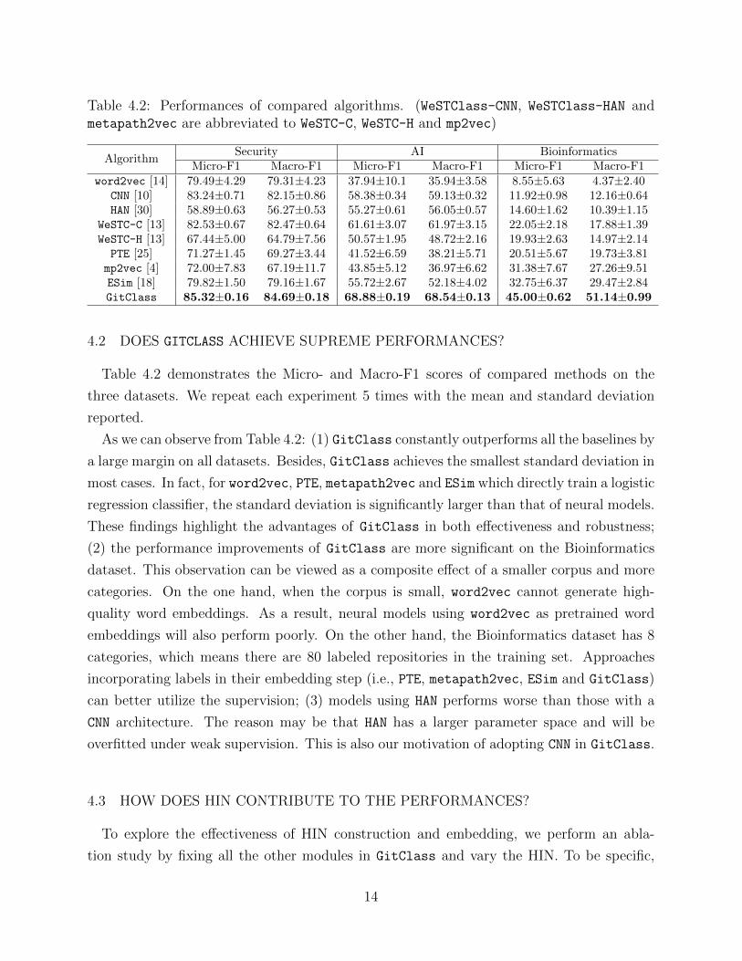
Table 4.2: Performances of compared algorithms. (WeSTClass-CNN, WeSTClass-HAN andmetapath2vec are abbreviated to WeSTC-C, WeSTC-H and mp2vec)
AlgorithmSecurity AI Bioinformatics
Micro-F1 Macro-F1 Micro-F1 Macro-F1 Micro-F1 Macro-F1word2vec [14] 79.49±4.29 79.31±4.23 37.94±10.1 35.94±3.58 8.55±5.63 4.37±2.40
CNN [10] 83.24±0.71 82.15±0.86 58.38±0.34 59.13±0.32 11.92±0.98 12.16±0.64HAN [30] 58.89±0.63 56.27±0.53 55.27±0.61 56.05±0.57 14.60±1.62 10.39±1.15
WeSTC-C [13] 82.53±0.67 82.47±0.64 61.61±3.07 61.97±3.15 22.05±2.18 17.88±1.39WeSTC-H [13] 67.44±5.00 64.79±7.56 50.57±1.95 48.72±2.16 19.93±2.63 14.97±2.14PTE [25] 71.27±1.45 69.27±3.44 41.52±6.59 38.21±5.71 20.51±5.67 19.73±3.81
mp2vec [4] 72.00±7.83 67.19±11.7 43.85±5.12 36.97±6.62 31.38±7.67 27.26±9.51ESim [18] 79.82±1.50 79.16±1.67 55.72±2.67 52.18±4.02 32.75±6.37 29.47±2.84GitClass 85.32±0.16 84.69±0.18 68.88±0.19 68.54±0.13 45.00±0.62 51.14±0.99
4.2 DOES GITCLASS ACHIEVE SUPREME PERFORMANCES?
Table 4.2 demonstrates the Micro- and Macro-F1 scores of compared methods on the
three datasets. We repeat each experiment 5 times with the mean and standard deviation
reported.
As we can observe from Table 4.2: (1) GitClass constantly outperforms all the baselines by
a large margin on all datasets. Besides, GitClass achieves the smallest standard deviation in
most cases. In fact, for word2vec, PTE, metapath2vec and ESim which directly train a logistic
regression classifier, the standard deviation is significantly larger than that of neural models.
These findings highlight the advantages of GitClass in both effectiveness and robustness;
(2) the performance improvements of GitClass are more significant on the Bioinformatics
dataset. This observation can be viewed as a composite effect of a smaller corpus and more
categories. On the one hand, when the corpus is small, word2vec cannot generate high-
quality word embeddings. As a result, neural models using word2vec as pretrained word
embeddings will also perform poorly. On the other hand, the Bioinformatics dataset has 8
categories, which means there are 80 labeled repositories in the training set. Approaches
incorporating labels in their embedding step (i.e., PTE, metapath2vec, ESim and GitClass)
can better utilize the supervision; (3) models using HAN performs worse than those with a
CNN architecture. The reason may be that HAN has a larger parameter space and will be
overfitted under weak supervision. This is also our motivation of adopting CNN in GitClass.
4.3 HOW DOES HIN CONTRIBUTE TO THE PERFORMANCES?
To explore the effectiveness of HIN construction and embedding, we perform an abla-
tion study by fixing all the other modules in GitClass and vary the HIN. To be specific,
14

74
77
80
83
86
Micro-F1
PTE as embedding
metapath2vec as embedding
No W-R-W
No W-U-W
No W-L-W
No W-W
Full
(a) Security, Micro-F1
70
74
78
82
86
Macro-F1
PTE as embedding
metapath2vec as embedding
No W-R-W
No W-U-W
No W-L-W
No W-W
Full
(b) Security, Macro-F1
57
60
63
66
69
Mic
ro-F
1
PTE as embedding
metapath2vec as embedding
No W-R-W
No W-U-W
No W-L-W
No W-W
Full
(c) AI, Micro-F1
53
57
61
65
69
Mac
ro-F
1
PTE as embedding
metapath2vec as embedding
No W-R-W
No W-U-W
No W-L-W
No W-W
Full
(d) AI, Macro-F1
30
34
38
42
46
Micro-F1
PTE as embedding
metapath2vec as embedding
No W-R-W
No W-U-W
No W-L-W
No W-W
Full
(e) Bioinformatics, Micro-F1
30
36
42
48
54
Macro-F1
PTE as embedding
metapath2vec as embedding
No W-R-W
No W-U-W
No W-L-W
No W-W
Full
(f) Bioinformatics, Macro-F1
Figure 4.1: Performances of algorithms with different HIN modules.
our HIN has four types of edges, each of which corresponds to a meta-path. We consider
four ablation versions (No W-W, No W-R-W, No W-L-W and No W-U-W). Each version ignores
one edge type/meta-path. Moreover, given the complete HIN, we consider to use PTE and
metapath2vec as our embedding technique, which generates two ablation versions PTE as
15

Table 4.3: Performances of algorithms with different keyword selection modules. tf-idf
uses the TFIDF score, while GitClass uses representativeness defined in Eqn. (3.7).
AlgorithmSecurity AI Bioinformatics
Micro-F1 Macro-F1 Micro-F1 Macro-F1 Micro-F1 Macro-F1tf-idf 85.12±0.22 84.50±0.25 68.91±0.20 68.02±0.23 41.49±0.56 45.10±1.58
GitClass 85.32±0.16 84.69±0.18 68.88±0.19 68.54±0.13 45.00±0.62 51.14±0.99
embedding and metapath2vec as embedding. Fig. 4.1 shows the performances of these
variants and the Full model.
From Fig. 4.1, we observe that: (1) our Full model outperforms the four ablation models
ignoring different edge types, indicating that each meta-path (as well as each node type incor-
porated in the HIN construction step) plays a positive role in the classification; (2) our Full
model outperforms PTE as embedding and metapath2vec as embedding, which validates
our choice of using ESim in the embedding step; (3) among the four ablation models ignor-
ing edge types, No W-R-W always performs the worst, which means W -R edges contribute
the most in repository classification. In contrast, W -W edges have the smallest offering.
This observation is aligned with the results in [25], where global/document-level word co-
occurrences are more helpful than local/context-level ones in document classification; (4) in
all cases, W -U edges (i.e., the user information) benefit the performances a lot. In the AI
and Bioinformatics datasets, user information is even more useful than label information.
This can be explained by the following statistics: in the AI dataset, there are 2,370 users
owning more than one repository, among which 1,777 users (65%) have all their repositories
in one category; in the Bioinformatics dataset, 108 pairs of repositories share the same user,
out of which 102 (94%) have the same topic label. These findings verify our claim that users
are strong indicators of topics.
4.4 HOW DOES KEYWORD EXTRACTION CONTRIBUTE TO THEPERFORMANCES?
We now proceed to the keyword extraction module. Recall that we propose a new repre-
sentativeness score considering both relevance and distinctiveness of a word in a category.
We study the effect of this module by comparing GitClass with its variant tf-idf, in which
the representativeness score is replaced by TFIDF (and all the other modules remain the
same). Quantitative results are shown in Table 4.3. In most cases, using representative-
ness achieves higher performances than using TFIDF. When there are more categories (e.g.,
the Bioinformatics dataset), the principle of distinctiveness helps more, resulting in a larger
16

Table 4.4: Top-10 words extracted by tf-idf and GitClass in keyword selection. We showthree categories here. Grey words are judged as not distinctive in the category.
Natural Language Processing Genetics Structural Bioinformatics
tf-idf GitClass tf-idf GitClass tf-idf GitClass
attention attention genotype genotype structures structuresseq2seq seq2seq igess igess pdb pdbtxt txt phenotype phenotype structure proteins
encoder encoder genetic geno proteins structuredecoder decoder devtools genetic protein pymollexicon lexicon matrix rqt pymol chaindiscourse discourse geno vcf chain excluded
size corpus rqt phenotypesimulator log knottycorpus snli vcf cohort cmake cmv
proceedings connectives simulation simulation knotty folding
boost of F1 scores.
We also conduct a qualitative comparison of the selected keywords. Table 4.4 lists top-
10 words selected by tf-idf and GitClass. We show three categories here, among which
Natural Language Processing comes from the AI dataset, while Genetics and Structural Bioin-
formatics are from the Bioinformatics dataset. In Table 4.4, several words extracted by
tf-idf are not distinctive (marked in grey). For example, “size” and “proceedings” are
not characteristic words of NLP. They may also appear in repositories related to CV and
Machine Learning. “devtools”, “log” and “cmake” are quite common words on GitHub. In-
cluding these words in the following topic modeling and pseudo document generation steps
will largely affect the quality of the synthesized training data. In contrast, GitClass ex-
cludes most common words. In Natural Language Processing, GitClass ranks “snli” (the
abbreviation of “Stanford Natural Language Inference” corpus) and “connectives” higher;
in Genetics, GitClass includes “phenotypesimulator” (a framework of simulating genotype to
phenotype relationships4) and “cohort”; in Structural Bioinformatics, an area mainly studying
the three-dimensional structure of biological macromolecules, “cmv” (a visualization tool of
protein5) and “folding” are ranked higher.
4.5 HOW DO PSEUDO DOCUMENTS CONTRIBUTE TO THE PERFORMANCES?
We generate 500 pseudo documents for each category in all previous experiments. What
if we use less/more synthesized training data? Intuitively, if we do not generate any pseudo
4https://github.com/HannahVMeyer/PhenotypeSimulator5https://github.com/eggzilla/cmv
17

75
78
81
84
87
90
0 500 1000 1500 2000
F1
#pseudo documents per class
Micro-F1
Macro-F1
(a) Security
55
60
65
70
75
0 500 1000 1500 2000
F1
#pseudo documents per class
Micro-F1
Macro-F1
(b) AI
20
30
40
50
60
0 500 1000 1500 2000
F1
#pseudo documents per class
Micro-F1
Macro-F1
(c) Bioinformatics
Figure 4.2: Performances of GitClass with different numbers of pseudo documents.
document, GitClass is equivalent to CNN with word embeddings pretrained by ESim. In
this way, signals learned in keyword extraction and topic modeling (i.e., spherical word
distribution of each class) cannot propagate to the training process. On the contrary, if we
have too many generated data, the training process will be inefficient. To see whether 500
is a good choice, we plot the performances of GitClass with 0, 10, 100, 500, 1000 and 2000
pseudo documents in Fig. 4.2.
On the one side, When the number of pseudo documents is too small (e.g., 0, 10 or
100), information carried in the synthesized training data will be insufficient to train a good
classifier. On the other side, when we generate too many pseudo documents (e.g, 1000
or 2000), putting efficiency aside, the performances are not guaranteed to increase. For
example, on the AI dataset, F1 scores fluctuate when the number of pseudo documents
becomes large; on Bioinformatics, they even drop. We believe this kind of drop results
from the fact that Bioinformatics has more categories, whose distributions are more likely
18

to overlap with each other on the sphere. Consequently, a certain number of documents
sampled from the overlapping area will confuse the classifier. In all, generating 500 to 1000
pseudo documents for each class will strike a good balance in our task.
19

CHAPTER 5: RELATED WORK
GitHub Repository Mining. Mining GitHub repositories is a long-lasting topic in soft-
ware engineering and social computing communities. Analytic studies [3, 28, 27, 9, 17] in-
vestigate how user activities (e.g., collaboration, following and watching) affect development
practice. Algorithmic studies [31, 19, 16] explore README files and repository metadata
to perform data mining tasks (e.g., similarity search [31] and clustering [19]). However, as
far as we know, previous studies have not explored automatic/weakly-supervised topic clas-
sification of GitHub repositories. In fact, some analyses [9, 17] rely on massive human effort
to annotate each repository. We hope the GitClass framework can trigger more interest in
automatic repository labeling.
HIN Mining. Many previous explorations focus on using meta-paths to conduct similarity
search [23, 20, 29] and node embedding [18, 4, 21] on HIN. From the view of applications,
several studies apply HIN node embeddings into downstream classification tasks, such as
malware detection [8] and medical diagnosis [7]. Different from the fully-supervised settings
in [8, 7], our repository classification task relies on a small set of user guidance. Moreover,
most information used in [8, 7] are structured. In contrast, signals in GitHub README
are buried under severe textual noises. GitClass overcomes these unique challenges by
introducing new techniques.
Weakly-Supervised Text Classification. Although deep neural architectures (e.g., CNN
[10] and HAN [30]) demonstrate their advantages in fully-supervised text classification, their
requirement of massive training data prohibits them from being adopted in some practi-
cal scenarios. Under weakly-supervised settings, there have been solutions following two
directions: (1) latent variable models, which extend topic models (e.g., PLSA and LDA) by
incorporating user-provided seed information [12, 2, 11]; and (2) embedding-based models,
which derives vectorized representations for words and documents [1, 25, 13]. However, all
these studies focus on text data without additional information. In GitClass, we are able
to go beyond plain text classification and utilize multi-modal signals.
20

CHAPTER 6: CONCLUSIONS AND FUTURE WORK
We presented GitClass, a framework to flexibly classify GitHub repositories under weak
supervision. To tackle the challenges of multi-modal signals, low data quality and limited
ground-truth, we integrate various techniques including HIN embedding, distinctive keyword
extraction and pseudo document generation. We demonstrate the effectiveness of GitClass
on three GitHub repository datasets. Moreover, we validate the design of our framework by
showing the positive contribution of each module.
There are still open issues with the design of GitClass. First, besides annotated reposito-
ries, users can provide the category name and several keywords for each class. It is interesting
to study how to effectively integrate different types of supervision to further boost the per-
formance of GitClass. Second, we assume that users only provide “one-round” guidance.
In practice, some users are willing to give feedback or multi-round supervision. In this way,
active learning techniques can be adopted to further improve the classification performances.
21

REFERENCES
[1] Ming-Wei Chang, Lev-Arie Ratinov, Dan Roth, and Vivek Srikumar. Importance ofsemantic representation: Dataless classification. In AAAI’08, pages 830–835, 2008.
[2] Xingyuan Chen, Yunqing Xia, Peng Jin, and John Carroll. Dataless text classificationwith descriptive lda. In AAAI’15, 2015.
[3] Laura Dabbish, Colleen Stuart, Jason Tsay, and Jim Herbsleb. Social coding in github:transparency and collaboration in an open software repository. In CSCW’12, pages1277–1286, 2012.
[4] Yuxiao Dong, Nitesh V Chawla, and Ananthram Swami. metapath2vec: Scalable rep-resentation learning for heterogeneous networks. In KDD’17, pages 135–144, 2017.
[5] Siddharth Gopal and Yiming Yang. Von mises-fisher clustering models. In ICML’14,pages 154–162, 2014.
[6] Aditya Grover and Jure Leskovec. node2vec: Scalable feature learning for networks. InKDD’16, pages 855–864, 2016.
[7] Anahita Hosseini, Ting Chen, Wenjun Wu, Yizhou Sun, and Majid Sarrafzadeh. Het-eromed: Heterogeneous information network for medical diagnosis. In CIKM’18, pages763–772, 2018.
[8] Shifu Hou, Yanfang Ye, Yangqiu Song, and Melih Abdulhayoglu. Hindroid: An intelli-gent android malware detection system based on structured heterogeneous informationnetwork. In KDD’17, pages 1507–1515, 2017.
[9] Eirini Kalliamvakou, Georgios Gousios, Kelly Blincoe, Leif Singer, Daniel M German,and Daniela Damian. The promises and perils of mining github. In MSR’14, pages92–101, 2014.
[10] Yoon Kim. Convolutional neural networks for sentence classification. In EMNLP’14,pages 1746–1751, 2014.
[11] Chenliang Li, Jian Xing, Aixin Sun, and Zongyang Ma. Effective document labelingwith very few seed words: A topic model approach. In CIKM’16, pages 85–94, 2016.
[12] Yue Lu and Chengxiang Zhai. Opinion integration through semi-supervised topic mod-eling. In WWW’08, pages 121–130, 2008.
[13] Yu Meng, Jiaming Shen, Chao Zhang, and Jiawei Han. Weakly-supervised neural textclassification. In CIKM’18, pages 983–992, 2018.
[14] Tomas Mikolov, Ilya Sutskever, Kai Chen, Greg S Corrado, and Jeff Dean. Distributedrepresentations of words and phrases and their compositionality. In NIPS’13, pages3111–3119, 2013.
22

[15] Bryan Perozzi, Rami Al-Rfou, and Steven Skiena. Deepwalk: Online learning of socialrepresentations. In KDD’14, pages 701–710, 2014.
[16] Gede Artha Azriadi Prana, Christoph Treude, Ferdian Thung, Thushari Atapattu, andDavid Lo. Categorizing the content of github readme files. Empirical Software Engi-neering, pages 1–32, 2018.
[17] Pamela H Russell, Rachel L Johnson, Shreyas Ananthan, Benjamin Harnke, and Nic-hole E Carlson. A large-scale analysis of bioinformatics code on github. PLOS One,13(10):e0205898, 2018.
[18] Jingbo Shang, Meng Qu, Jialu Liu, Lance M Kaplan, Jiawei Han, and Jian Peng. Meta-path guided embedding for similarity search in large-scale heterogeneous informationnetworks. arXiv preprint arXiv:1610.09769, 2016.
[19] Abhishek Sharma, Ferdian Thung, Pavneet Singh Kochhar, Agus Sulistya, and DavidLo. Cataloging github repositories. In EASE’17, pages 314–319, 2017.
[20] Yu Shi, Po-Wei Chan, Honglei Zhuang, Huan Gui, and Jiawei Han. Prep: Path-basedrelevance from a probabilistic perspective in heterogeneous information networks. InKDD’17, pages 425–434, 2017.
[21] Yu Shi, Qi Zhu, Fang Guo, Chao Zhang, and Jiawei Han. Easing embedding learning bycomprehensive transcription of heterogeneous information networks. In KDD’18, pages2190–2199, 2018.
[22] Yizhou Sun and Jiawei Han. Mining heterogeneous information networks: principles andmethodologies. Synthesis Lectures on Data Mining and Knowledge Discovery, 3(2):1–159, 2012.
[23] Yizhou Sun, Jiawei Han, Xifeng Yan, Philip S Yu, and Tianyi Wu. Pathsim: Metapath-based top-k similarity search in heterogeneous information networks. PVLDB,4(11):992–1003, 2011.
[24] Yizhou Sun, Yintao Yu, and Jiawei Han. Ranking-based clustering of heterogeneousinformation networks with star network schema. In KDD’09, pages 797–806. ACM,2009.
[25] Jian Tang, Meng Qu, and Qiaozhu Mei. Pte: Predictive text embedding through large-scale heterogeneous text networks. In KDD’15, pages 1165–1174, 2015.
[26] Jian Tang, Meng Qu, Mingzhe Wang, Ming Zhang, Jun Yan, and Qiaozhu Mei. Line:Large-scale information network embedding. In WWW’15, pages 1067–1077, 2015.
[27] Jason Tsay, Laura Dabbish, and James Herbsleb. Influence of social and technicalfactors for evaluating contribution in github. In ICSE’14, pages 356–366. ACM, 2014.
[28] Jason T Tsay, Laura Dabbish, and James Herbsleb. Social media and success in opensource projects. In CSCW’12, pages 223–226, 2012.
23
[29] Carl Yang, Mengxiong Liu, Frank He, Xikun Zhang, Jian Peng, and Jiawei Han.Similarity modeling on heterogeneous networks via automatic path discovery. InECML/PKDD’18, pages 37–54, 2018.
[30] Zichao Yang, Diyi Yang, Chris Dyer, Xiaodong He, Alex Smola, and Eduard Hovy.Hierarchical attention networks for document classification. In NAACL’16, pages 1480–1489, 2016.
[31] Yun Zhang, David Lo, Pavneet Singh Kochhar, Xin Xia, Quanlai Li, and Jianling Sun.Detecting similar repositories on github. In SANER’17, pages 13–23, 2017.
24


