c©Copyright 2012

Anna Klimova

Coordinate-Free Exponential Families on Contingency Tables

Anna Klimova

A dissertation submitted in partial fulfillmentof the requirements for the degree of

Doctor of Philosophy

University of Washington

2012

Reading Committee:

Tamas Rudas, Chair

Thomas S. Richardson, Chair

Rekha R. Thomas

Program Authorized to Offer Degree:Statistics

University of Washington

Abstract

Coordinate-Free Exponential Families on Contingency Tables

Anna Klimova

Chair of the Supervisory Committee:Professor Tamas Rudas

Department of Statistics, Eotvos Lorand University, Budapest, Hungary

Professor Thomas S. RichardsonDepartment of Statistics, University of Washington

We propose a class of coordinate-free multiplicative models on the set of positive distri-

butions on contingency tables and on some sets of cells of a more general structure. The

models are called relational and are generated by subsets of cells, some of which may not

be induced by marginals of the table. Under the model, every cell parameter is the product

of effects associated with subsets the cell belongs to. Such models are useful in analyz-

ing incomplete tables and generalized independence structures not pertaining to subsets of

variables forming the table.

We reveal when a relational model is regular or else a curved exponential family. We

establish necessary and sufficient conditions for the existence and uniqueness of the MLE in

the curved case. We also determine the conditions under which the properties of the MLE

under relational models are comparable to those under hierarchical log-linear models and

prove a generalization of Birch’s theorem.

We propose a generalization of the iterative proportional fitting procedure that can be

used for maximum likelihood estimation under relational models and prove its convergence.

Finally, we use the relational model framework to contribute to the ongoing debate as

to whether British social mobility is declining and compare the patterns of occupational

mobility in Great Britain in 1991 and 2005.

TABLE OF CONTENTS

Page

List of Figures . . . . . . . . . . . . . . . . . . . . . . . . . . . . . . . . . . . iii

Chapter 1: Introduction . . . . . . . . . . . . . . . . . . . . . . . . . . . . 1

1.1 Background . . . . . . . . . . . . . . . . . . . . . . . . . . . . . . . . 1

1.2 Motivation . . . . . . . . . . . . . . . . . . . . . . . . . . . . . . . . . 6

1.3 Main Results and Thesis Structure . . . . . . . . . . . . . . . . . . . 11

Chapter 2: Relational Models for Contingency Tables . . . . . . . . . . . . 14

2.1 Definition and Log-linear Representation of Relational Models . . . . 15

2.2 Parameterizations and Degrees of Freedom . . . . . . . . . . . . . . . 19

2.3 Relational Models as Exponential Families . . . . . . . . . . . . . . . 25

2.4 Mixed Parameterization of Exponential Families . . . . . . . . . . . . 29

Chapter 3: Maximum Likelihood Estimation for Relational Models . . . . . 34

3.1 Poisson vs Multinomial Sampling . . . . . . . . . . . . . . . . . . . . 37

3.2 Existence and Properties of the Maximum Likelihood Estimates . . . 41

3.3 Birch’s Theorem and the Geometry of Relational models . . . . . . . 45

3.4 Numerical Solution of Likelihood Equations . . . . . . . . . . . . . . 48

3.5 Iterative Proportional Fitting . . . . . . . . . . . . . . . . . . . . . . 53

Chapter 4: Coordinate Free Comparative Analysis of Social Mobility . . . . 67

4.1 Data and Previous Analyses . . . . . . . . . . . . . . . . . . . . . . . 74

4.2 Relational Models of Social Mobility . . . . . . . . . . . . . . . . . . 77

4.3 Results . . . . . . . . . . . . . . . . . . . . . . . . . . . . . . . . . . . 82

Appendix A: Maximum Likelihood Estimation Using R . . . . . . . . . . . . 85

A.1 The Newton-Raphson Method: Models for Intensities . . . . . . . . . 85

i

A.2 The Aitchison-Silvey Method: Models for Probabilities . . . . . . . . 87

A.3 Generalized Iterative Proportional Fitting . . . . . . . . . . . . . . . 89

A.4 Computation of a Kernel Basis Matrix . . . . . . . . . . . . . . . . . 92

Appendix B: Examples . . . . . . . . . . . . . . . . . . . . . . . . . . . . . . 94

B.1 Bait Study for Swimming Crabs . . . . . . . . . . . . . . . . . . . . . 94

B.2 Pneumonia Infection in Calves . . . . . . . . . . . . . . . . . . . . . . 96

B.3 Testing Independence of Attributes . . . . . . . . . . . . . . . . . . . 97

ii

LIST OF FIGURES

Figure Number Page

2.1 The canonical parameter space in Example 1.2.3. . . . . . . . . . . . 28

4.1 Estimated mobility effects under Mdiff. . . . . . . . . . . . . . . . . . 84

iii

ACKNOWLEDGMENTS

Here, I would like to say thank you to all the people who supported me through

the journey of this thesis. My journey was not smooth sailing, but with their generous

help I was able to arrive safely to where I am now.

First of all, I thank my advisors, Tamas Rudas and Thomas Richardson who

trusted in me, stayed by my side, and helped me to develop statistical intuition and

to become a statistician. Tamas exposed me to the world of categorical data analysis,

guided me through the whole journey, and influenced the way I think about statistics.

Thomas followed up with my student progress and steered me toward getting practical

experience and successful graduation.

This thesis required some knowledge from other fields of study, and my thesis

committee members assisted me with acquiring that. I thank Rekha Thomas for in-

troducing me to algebraic geometry and reading this thesis. I express my appreciation

to Adrian Dobra for helping me learn statistical computing and for financial support

through NIH Grant R01 HL092071. I also thank my GSR Brian Flaherty for his

comments and suggestions during my examinations.

From the very first day at the department I felt encouragement and support from

Michael Perlman who mentored me for all five years. My deepest gratitude to Michael

for creating arrangements that made the whole graduate school possible for me.

Marina Meila gave me a unique experience in her incredible class on statistical

learning and advised me on the computing project. I am very thankful to Marina for

inspiring me when it was especially needed.

I was fortunate to have my thesis work and related travel supported by Grant No

iv

TAMOP 4.2.1./B-09/1/KMR-2010-0003 from the European Union and the European

Social Fund, and by a Graduate Student Research Presentation and Training Grant

from the Center for Statistics and the Social Sciences (University of Washington).

Finally, I want to thank my dear friends, Anna Burago and Elena Petrunina, and

my mother in law, Mrs. Olga Klimova. It takes a village to raise a child, and these

wonderful women helped create that village for my children.

v

1

Chapter 1

INTRODUCTION

1.1 Background

The main objective of this dissertation is to develop a new class of models on the set

of positive distributions on contingency tables and on some sets of cells that have a

more general structure. The proposed models generalize hierarchical log-linear models

and retain some of their properties. An overview of hierarchical log-linear models and

of the main results concerning maximum likelihood estimation under such models is

given in this section.

Let Y1, . . . , YK be discrete random variables modeling certain characteristics of

the population of interest, and let Y1, . . . ,YK denote the individual ranges of the

variables. The set I = Y1× · · · ×YK corresponds to a classical complete contingency

table, and a point (y1, y2, . . . , yK) ∈ Y1 × · · · × YK is called a cell.

A subset M ⊂ Y1, Y2, . . . , YK specifies a marginal of the contingency table, and

the Cartesian product of Yk’s such that Yk ∈ M is referred to as the M -marginal

table. The subset of cells in I whose coordinate projections into the M -marginal

table are identical form a cylinder set. The cylinder sets, corresponding to the same

marginal, partition the table I.

Depending on the procedure that generates data on I, the population may be

characterized by cell probabilities or cell intensities. The parameters of the true

distribution will be denoted by δ = δ(i), for i ∈ I. In the case of probabilities,

δ(i) = p(i) ∈ (0, 1), where∑

i∈I p(i) = 1; in the case of intensities, δ(i) = λ(i) > 0.

Write P = Pδ : δ ∈ Ω for the set of all positive distributions on the table

I. Here the parameter space Ω is an open subset of R|I|>0. For some Θ ⊂ Ω, the set

2

PΘ = Pδ ∈ P : δ ∈ Θ is a model in P .

An ordinary (hierarchical) log-linear model (cf. Haberman, 1974; Bishop et al.,

1975; Agresti, 2002) is specified by some marginals of the contingency table. Under

the model, each log cell parameter is equal to the sum of the effects associated with

the marginals that generate the model and of the effects associated with all subsets

of those marginals.

Definition 1.1.1. Let M = M1, . . . ,MG be a class of marginals, and let C1, C2, . . . , CJ

be the list of all cylinder sets induced by the marginals in M and by all of their subsets.

Let |I| = card(I) and A be a J × |I| matrix with entries

aji = Ij(i) =

1 if the cell i is in Cj,

0 otherwise,for i = 1, . . . , |I| and j = 1, . . . , J. (1.1)

A hierarchical log-linear model generated by the class M is the following subset of P :

Pδ ∈ P : log δ = A′β for some β ∈ RJ. (1.2)

Here β is the vector of log-linear parameters of the model and A is the model

matrix.

The definition (1.2) does not refer explicitly to the dimensions of variables forming

the table I and thus is coordinate-free. A coordinate-free representation of a log-

linear model was introduced in the analysis of categorical data by Haberman (1974).

A similar definition of a log-linear model is employed in algebraic statistics, where

log-linear models are a special case of toric models (cf. Pachter & Sturmfels, 2005;

Drton et al., 2009).

The dual representation of a hierarchical log-linear model is obtained by describing

the association structure of the distributions in the model in terms of the odds ratios.

The minimal number of odds ratios required to specify a log-linear model is equal to

the number of degrees of freedom of this model (cf. Bishop et al., 1975).

3

Example 1.1.1. Let I = (0, 0), (0, 1), (1, 0), (1, 1) be the sequence of cells of the

2× 2 contingency table, Y1, Y2 be random variables each taking values in 0, 1, and

p = (p11, p12, p21, p22)′ be the vector of positive probabilities (in the usual notation).

The model of independence of Y1 and Y2, expressed as

p11p22

p12p21

= 1,

is a log-linear model, generated by the empty marginal (the whole table), the row

marginal Y1, and the column marginal Y2. The distribution, parameterized by p, is

in the model of independence if and only if

log p =

1 1 0 1 0

1 1 0 0 1

1 0 1 1 0

1 0 1 0 1

β1

β2

β3

β4

β5

,

where β = (β1, β2, β3, β4, β5)′ is the vector of parameters, associated with the cylinder

sets: the whole table, the two rows, and the two columns, respectively.

Hierarchical log-linear models are conventional in categorical data analysis and, in

the sequel, the word hierarchical is omitted.

Under the model (1.2) the cell parameters can be written in the form:

δ(i) = exp J∑j=1

Ij(i)βj, for i ∈ I. (1.3)

Therefore, a log-linear model is an exponential family of distributions, with the canon-

ical parameters βj’s and the canonical statistics equal to indicators Ij of the cylinder

sets. It can be shown that the canonical parameters can be expressed in terms of log

odds ratios (cf. Bishop et al., 1975, p.17). A log-linear model induces a mixed param-

4

eterization on the set of all complete contingency tables of the same structure as the

table I. The canonical parameters are the odds ratios, and the mean-value parame-

ters are the marginal totals. Since a log-linear model is a regular exponential family,

the observed marginal distributions and the odds ratios are variation independent

and uniquely specify a contingency table (Barndorff-Nielsen, 1978, p.122).

The Poisson and multinomial sampling schemes are often used to collect categori-

cal data, and the relationship between Poisson and multinomial maximum likelihood

estimators under log-linear models was studied in detail by Birch (1963), Haberman

(1974), Bishop et al. (1975), among others. The main result about this relationship

is stated in the following theorem.

Theorem 1.1.1. (Haberman, 1974, p.41) For a given set of observations, the max-

imum likelihood estimates under a log-linear model for intensities and under a log-

linear model for probabilities, generated by the same class of marginals, are equal.

Bishop, Fienberg, & Holland (1975) give a finer statement about the equivalence

of the Poisson and multinomial MLEs:

Theorem 1.1.2. For a given set of observations, the maximum likelihood estimates

under a log-linear model for intensities and under a log-linear model for probabilities,

generated by the same class of marginals, are equal if and only if the total of the MLE

under the model for intensities is the same as the sample size used for multinomial

sampling.

Theorem 1.1.2 implicitly says that the MLEs are equal if and only if the total of

the MLE under the model for intensities is the same as the observed total. The latter

always holds under a hierarchical log-linear model.

The conditions of existence and uniqueness of the maximum likelihood estimates

under log-linear models were studied by Birch (1963), Andersen (1974), and Haber-

man (1974), among others. Positivity of all observed cell frequencies is sufficient for

5

the existence of the MLE, see, e.g., Corollary 2.1 (Haberman, 1974, p.38). It was also

proved that the maximum likelihood estimates exist if and only if the vector of the

mean-value parameters (the integrals of the canonical statistics) is contained in the

interior of the convex hull of the support of its distribution (cf. Andersen, 1974).

Another fundamental result establishes the equality between the mean-value pa-

rameters of the MLE and the mean-value parameters of the observed distribution:

Theorem 1.1.3. (Birch, 1963)

• The marginal totals are sufficient statistics for the parameters of the model.

• The marginal totals are equal to the maximum-likelihood estimates of their expectations.

• There exists a unique set of values of cell parameters that satisfies both the model

and the likelihood equations.

• The maximum-likelihood estimates are determined uniquely by the marginal totals

being equal to the maximum-likelihood estimates of their expectations.

Birch’s theorem implies that the maximum likelihood estimates for the cell pa-

rameters under a log-linear model can be computed directly, without first calculating

the parameters of the model. Such computation can be performed, e.g., using the

iterative proportional fitting (IPF) procedure that finds a set of frequencies satisfying

both the model and the likelihood equations (cf. Bishop et al., 1975). By Birch’s

theorem, this set of frequencies is unique and constitutes the MLE under the model.

Log-linear models are widely applied in categorical data analysis (cf. Bishop et al.,

1975; Agresti, 2002), but they have some limitations. For example, a conventional log-

linear model does not capture characteristics, other than marginal effects, that some

cells may have in common. Consequently, there has always been interest in models

that also allow for multiplicative effects that are associated with those characteristics.

The statistical problems, in which such models arise, motivated this work and will be

described in the next section.

6

1.2 Motivation

Models that allow for multiplicative effects not associated with the marginals in the

table were originally proposed in social mobility research. Social mobility is a tran-

sition of an individual from one social position to another in a stratified society. A

common approach to the analysis of social mobility is based on social mobility tables

that cross-classify individuals, typically men, according to their own and their father’s

social status. The model of perfect mobility, i.e., independence between Father’s sta-

tus and Son’s status, does not fit most data sets, because too many sons retain their

father’s status. To account for status inheritance, models of “quasi-perfect mobility”,

that include additional parameters for diagonal cells, were proposed by White (1963)

and Goodman (1965). Later, a number of models that express specific patterns of

association in mobility tables were introduced (Goodman, 1969). A model, called

topological, that accounts for an arbitrary pattern of association in a mobility table,

was proposed by Hauser (1978). Under such a model, the log cell probabilities are

sums of the effects associated with fathers’ and sons’ statuses and the interaction

effects, which are assumed to be identical for all cells that belong to the same level.

Hauser’s levels are subsets of cells that partition the mobility table; the cells in the

same subset are characterized by the similar levels of mobility between fathers’ and

sons’ statuses.

The model of quasi-independence introduced by Goodman (1968) for mobility

tables can also be used for the analysis of incomplete tables, in which some of the

combinations (y1, y2, . . . , yK) ∈ Y1 × · · · × YK do not logically exist or do not appear

in a particular population. Goodman (1968) pointed out that the concept of quasi-

independence “leads to methods that focus attention in turn on various subsets of the

entire table, making possible a more detailed analysis of the association between the

row and column classifications in the table”.

The parameters associated with subsets, that are not cylinder sets, are also in-

7

Table 1.1: Diagnoses of Psychiatric Patients. S - schizophrenic; NS - not schizophrenic(Tanner & Young, 1985a).

Flexible 6Schneider, S Schneider, NS

Taylor S NS S NSS 19 14 11 14

NS 7 15 15 101

cluded in models of agreement or disagreement between raters (cf. Tanner & Young,

1985a,b).

Example 1.2.1. Young, Tanner, & Meltzer (1982) describe a study that aimed to

compare the agreement between different systems of diagnosing schizophrenia for 196

patients. The diagnoses of the patients produced by the systems Flexible 6, Schneider,

and Taylor, are summarized in Table 1.1. Pairwise agreement can be expressed using

three subsets of cells - S1 (the agreement between Flexible 6 and Schneider systems),

S2 (the agreement between Flexible 6 and Taylor systems), and S3 (the agreement

between Schneider and Taylor systems):

S1 = (0, 0, 0), (0, 0, 1), (1, 1, 0), (1, 1, 1),

S2 = (0, 0, 0), (0, 1, 0), (1, 0, 1), (1, 1, 1),

S3 = (0, 0, 0), (1, 0, 0), (0, 1, 1), (1, 1, 1).

The model of non-homogeneous pairwise agreement within three pairs of raters has

independence as the baseline model and, in addition, includes parameters associated

with the subsets of cells corresponding to pairwise agreement:

log p(i, j, k) = α + α(Flex)i + α

(Schn)j + α

(Tayl)k +

δ1I1(i, j, k) + δ2I2(i, j, k) + δ3I3(i, j, k), (1.4)

8

where i, j, k ∈ 0, 1 and

It(i, j, k) =

1 if (i, j, k) ∈ St,

0 otherwise,

for t = 1, 2, 3. The parameters α, α(Flex)i , α

(Schn)j , and α

(Tayl)k are associated with the

cylinder sets induced by the marginals in the table, but the parameters δ1, δ2, and δ3

are associated with non-cylinder sets.

The model (1.4) is the log-linear model associated with the matrix A, where

A =

1 1 1 1 1 1 1 1

1 1 1 1 0 0 0 0

0 0 0 0 1 1 1 1

1 1 0 0 1 1 0 0

0 0 1 1 0 0 1 1

1 0 1 0 1 0 1 0

0 1 0 1 0 1 0 1

1 1 0 0 0 0 1 1

1 0 1 0 0 1 0 1

1 0 0 1 1 0 0 1

.

The representation (1.2) is a primal representation of a hierarchical log-linear

model. The dual representation of such a model is obtained by setting certain odds

ratios equal to one. Some other models, like the one described in the following ex-

ample, are intrinsically specified by multiplicative constraints on the cell parameters,

but the constraints cannot be expressed in terms of the odds ratios.

Example 1.2.2. The study described by Kawamura et al. (1995) compared three

bait types for trapping swimming crabs: fish alone, sugarcane alone, and sugarcane-

fish combination. The study intended to show that the sugarcane-fish combination

9

Table 1.2: Poisson intensities by bait type.

FishSugarcane Yes No

Yes λ11 λ01

No λ10 -

was the most effective bait, and, during the experiment, catching crabs without bait

was not considered. The population structure can be expressed as an incomplete

contingency table, and three Poisson random variables can be used to model the

number of crabs caught in the three traps. The notation for the intensities is shown

in Table 1.2. The model assuming that there is a multiplicative effect of using both

bait types at the same time can be expressed as

λ11 = λ01λ10. (1.5)

Each cell belongs to at least one of the two subsets - S1 (sugarcane is added to bait) or

S2 (fish is added to bait). Then, if β1 and β2 are the log-linear parameters associated

with those subsets, the model can be written in the form (1.2):

log

λ11

λ01

λ10

=

1 1

1 0

0 1

β1

β2

.

Subsets of cells arise naturally in any model under which the cell parameters are

expressed as the product of fewer parameters: each parameter in the model has a

subset of cells associated with it. Such a model can also be written in the log-linear

form (1.2), but the model matrix may include entries other than 0 or 1, unlike the

10

model matrix for a hierarchical log-linear model. A model of this kind appears in the

example below.

Example 1.2.3. Agresti (2002) describes a study carried out to determine if a pneu-

monia infection has an immunizing effect on dairy calves. Within 60 days after birth,

the calves were exposed to a pneumonia infection. The calves that got the infec-

tion were then classified according to whether or not they got the secondary infection

within two weeks after the first infection cleared up. The number of the infected calves

is thus a random variable with the multinomial distribution M(N, (p11, p12, p22)′),

where N denotes the total number of calves in the sample. Suppose further that

p11 is the probability to get both the primary and the secondary infection, p12 is the

probability to get only the primary infection and not the secondary one, and p22 is the

probability not to catch either the primary or the secondary infection. Let 0 < π < 1

denote the probability to get the primary infection. The hypothesis of no immunizing

effect of the primary infection is expressed as (cf. Agresti, 2002)

p11 = π2, p12 = π(1− π), p22 = 1− π, (1.6)

or, in the log-linear form:

log

p11

p12

p22

=

2 0

1 1

0 1

β1

β2

, (1.7)

where β1 = log π and β1 = log (1− π).

The models brought up in this section are applied in different contexts and speci-

fied either in a log-linear or in a multiplicative form. In an explicit or implicit way, a

multiplicative model is generated by a class of subsets of cells, some of which may not

be induced by marginals of the table; under the model every cell parameter can be

11

written as the product of effects associated with those subsets which the cell belongs

to. The idea of a model generated by a class of subsets of cells was formalized in

the relational model framework, proposed by Klimova, Rudas, & Dobra (2012) and

described in detail in this dissertation.

1.3 Main Results and Thesis Structure

A relational model generated by a class of subsets of cells is formally introduced in

Chapter 2, Section 2.1. Relational models can be considered for discrete distributions

on the sets of cells that have a more general structure than a complete contingency

table. Log-linear models are a special case of relational models, and the properties of

relational models may be expected to be comparable to those of traditional log-linear

models. The degrees of freedom and the dual representation of relational models

are discussed in Section 2.2: every relational model can be stated in terms of the

generalized odds ratios; the minimal number of generalized odds ratios required to

specify the model is equal to the number of degrees of freedom of this model. The

row space of the model matrix does not depend on parameterization and is called the

design space of the model.

In Section 2.3, it is shown that all relational models for intensities are regular ex-

ponential families. Relational models for probabilities are regular exponential families

only if the row of all 1’s is in the design space of the model. Otherwise, the models

for probabilities are curved exponential families.

A mixed parameterization of finite discrete exponential families is discussed in

Section 2.4. Any relational model is naturally defined under a parameterization of

this kind: the corresponding generalized odds ratios are fixed and the model is pa-

rameterized by the remaining mean-value parameters. The parameters, that describe

the distributions of observed values of subset sums, and generalized odds ratios are

variation independent and, in the regular case, specify the table uniquely.

The properties of relational models as exponential families are discussed further

12

in Chapter 3. An extension of Theorem 1.1.2 to relational models is proved in Section

3.1. Given the model matrix is the same, the following four conditions are equivalent:

the maximum likelihood estimates for the cell frequencies under a model for intensities

and under a model for probabilities are equal, the row of 1’s is in the design space

of the model, the model may be defined by homogeneous odds ratios, the model

for intensities is scale-invariant. It is well known that all four conditions hold for a

hierarchical log-linear model. The overall effect, associated with the whole table as

the empty marginal, is always included in such a model and thus the design space

contains the row of 1’s. Similarly, relational models with the vector of all 1’s in the

design space are referred to as models with the overall effect.

All relational models for intensities and the models for probabilities with the

overall effect are discrete regular exponential families, and the MLE under such models

exists and is unique if only if all mean-value parameters of the observed distribution

are positive (cf. Barndorff-Nielsen, 1978). Relational models for probabilities without

the overall effect are curved exponential families. It will be proved in Section 3.2 that

the maximum likelihood estimates in the curved case exist and are unique under the

same condition as for discrete regular exponential families.

An extension of Birch’s theorem to regular exponential families (cf. Barndorff-

Nielsen, 1978) implies that under all relational models for intensities and under re-

lational models for probabilities with the overall effect the mean-value parameters of

the MLE, given it exists, are equal to the corresponding mean-value parameters of the

observed distribution. However, Birch’s theorem does not hold for relational models

for probabilities without the overall effect. Under such models, the mean-value pa-

rameters of the MLE are proportional to the corresponding mean-value parameters

of the observed distribution, and the coefficient of proportionality depends on the

observed distribution.

A generalization of Birch’s theorem that applies to all relational models, whether

or not they are regular exponential families, is proved in Section 3.3: a relational

13

model imposes an equivalence relation on the set of all positive distributions, and

the equivalence classes consist of the distributions that have the same MLE. The

equivalence classes are given a geometric interpretation, and the parameter space and

relational models are described in terms of algebraic geometry.

A previously unpublished generalization of IPF is proposed in Section 3.5. The

IPF(γ) algorithm can be used for maximum likelihood estimation under all relational

models for intensities, for all relational models for probabilities with the overall effect,

and, in some cases, for models for probabilities without the overall effect. The G-IPF

algorithm, built on IPF(γ), is primarily intended for relational models for probabilities

without the overall effect, but can be used for all relational models. The proofs of

convergence of the IPF(γ) and G-IPF algorithms are given as well.

In Chapter 4, the relational models framework is used for the analysis of trends in

social mobility (Klimova & Rudas, 2012). The analysis is based on the employment

data from the 1991 British Household Panel Survey and the 2005 General Household

Survey. Mobility is categorized by the number of steps up or down from the father’s

position, forming mobility bands parallel to the main diagonal in the mobility table.

The relational models proposed by Klimova & Rudas (2012) have conditional inde-

pendence of the father’s and son’s position given year as the baseline model and, in

addition, include effects associated with the mobility bands. The maximum likeli-

hood estimates are obtained using the IPF(γ) algorithm described in Chapter 3. The

results are discussed in Section 4.3.

The algorithms, described in Sections 3.4 and 3.5, are implemented in R (R De-

velopment Core Team, 2010), and the computer code is provided in the Appendix.

14

Chapter 2

RELATIONAL MODELS FOR CONTINGENCY TABLES

Introduction

This chapter introduces a new class of models for the set of positive distributions on

contingency tables and on some sets of cells that have a more general structure.

A relational model is generated by a class of subsets of cells, some of which may

not be induced by marginals of the table; under the model, every cell parameter is

the product of effects associated with those subsets which the cell belongs to. The

definition of the relational model is given in Section 2.1 and is illustrated by several

examples. The degrees of freedom and the dual representation of relational models are

discussed in Section 2.2. Every relational model can be stated in terms of generalized

odds ratios. The minimal number of generalized odds ratios required to specify the

model is equal to the number of degrees of freedom of this model.

Relational models are exponential families of distributions. Some of their proper-

ties as exponential families are discussed in Section 2.3. The models for probabilities

that include the overall effect and all relational models for intensities are regular ex-

ponential families. Relational models for probabilities without the overall effect are

curved exponential families (Efron, 1975; Brown, 1988; Kass & Vos, 1997).

A mixed parameterization of a finite discrete exponential family is discussed in

Section 2.4. The canonical parameters are the generalized odds ratios, and the mean-

value parameters are the subset sums. Any relational model is naturally defined via

this parameterization: the corresponding generalized odds ratios are fixed and the

model is parameterized by remaining mean-value parameters. The parameters, that

describe the distributions of observed values of subset sums, and generalized odds

15

ratios are variation independent and, in the regular case, specify the table uniquely.

2.1 Definition and Log-linear Representation of Relational Models

In this section, the relational model class will be introduced using notation that was

described in Section 1.1. As before, Y1, . . . , YK denote the discrete random variables

with ranges Y1, . . . ,YK respectively. Assume further that a point (y1, y2, . . . , yK) ∈

Y1 × · · · × YK generates a cell if and only if the outcome (y1, y2, . . . , yK) appears in

the population. A combination (y1, y2, . . . , yK) that does not exist logically, does not

appear in a particular population, or was not included in the experiment design is

referred to as an empty cell. The lexicographically ordered set I of non-empty cells

in Y1×· · ·×YK is called a table. The parameters of the true distribution are denoted

by δ = δ(i), for i ∈ I, and P = Pδ : δ ∈ Ω stands for the set of positive

distributions on I.

Definition 2.1.1. Let S = S1, . . . , SJ be a class of non-empty subsets of the table

I and A be a J × |I| matrix with entries

aji = Ij(i) =

1, if the i-th cell is in Sj,

0, otherwise,for i = 1, . . . , |I| and j = 1, . . . , J.

(2.1)

A relational model RM(S) with the model matrix A is the following subset of P :

RM(S) = Pδ ∈ P : log δ = A′β, for some β ∈ RJ. (2.2)

Under the model (2.2) the parameters of the distribution can also be written as

δ(i) = exp J∑j=1

Ij(i)βj =J∏j=1

(θj)Ij(i), (2.3)

where θj = exp (βj), for j = 1, . . . , J .

16

The parameters β in (2.2) are called the log-linear parameters. The parameters

θ in (2.3) are called the multiplicative parameters. If the subsets in S are cylinder

sets, the parameters β coincide with the parameters of the corresponding log-linear

model.

In the case δ = p it must be assumed that ∪Jj=1Sj = I, i.e. there are no zero

columns in the matrix A. A zero column implies that one of the probabilities is 1

under the model and the model is thus trivial.

The example below describes a model of conditional independence as a relational

model.

Example 2.1.1. Consider the model of conditional independence [Y1Y3][Y2Y3] of three

binary variables Y1, Y2, Y3, each taking values in 0, 1. The model is expressed as

pijk =pi+kp+jk

p++k

,

where pi+k, p+jk, p++k are marginal probabilities in the standard notation (Bishop et

al., 1975). Let S be the class consisting of the cylinder sets associated with the empty

marginal and with the marginals Y1, Y2, Y3, Y1Y3, Y2Y3. The “raw” model matrix

Araw can be computed from (2.1), and

A′raw =

1 1 0 1 0 1 0 1 0 0 0 1 0 0 0

1 1 0 1 0 0 1 0 1 0 0 0 1 0 0

1 1 0 0 1 1 0 1 0 0 0 0 0 1 0

1 1 0 0 1 0 1 0 1 0 0 0 0 0 1

1 0 1 1 0 1 0 0 0 1 0 1 0 0 0

1 0 1 1 0 0 1 0 0 0 1 0 1 0 0

1 0 1 0 1 1 0 0 0 1 0 0 0 1 0

1 0 1 0 1 0 1 0 0 0 1 0 0 0 1

. (2.4)

The matrix Araw is not full row rank, and thus the model parameters are not iden-

tifiable (cf. Section 2.2). A full row rank model matrix can be obtained by setting,

17

for instance, the level 0 of each variable as the reference level. After that, the model

matrix is equal to

A =

1 1 1 1 1 1 1 1

0 0 0 0 1 1 1 1

0 0 1 1 0 0 1 1

0 1 0 1 0 1 0 1

0 0 0 0 0 1 0 1

0 0 0 1 0 0 0 1

. (2.5)

The first row corresponds to the cylinder set associated with the empty marginal.

The next three rows correspond to the cylinder sets generated by the level 1 of Y1,

Y2, Y3 respectively. The fifth row corresponds to the cylinder set generated by the

level 1 for both Y1 and Y3, and the last row - to the cylinder set corresponding to the

level 1 for both Y2 and Y3.

In the next example, one of the cells in the Cartesian product of the ranges of the

variables is empty and the sample space I is a proper subset of this product.

Example 1.2.2 (Revisited)

The model assuming that there is a multiplicative effect of using both bait types at

the same time is a relational model for intensities generated by the class S = S1, S2,

where S1 = (0, 0), (0, 1) and S2 = (0, 0), (1, 0). Under the model,

log λ = A′β,

where

A =

1 1 0

1 0 1

and β = (β1, β2)′. The relationship between the two representations of the model will

be explored in the next section.

18

The following example features relational models as a potential tool for modeling

social mobility tables. A model of independence is considered on a space that is not

the Cartesian product of the ranges of the variables in the table.

Example 2.1.2. A cross-classification given in Table 2.1 (Blau & Duncan, 1967) ex-

presses a relation between occupational statuses of respondents and of their fathers

and constitutes a social mobility table. To test the hypothesis of independence be-

tween respondent’s mobility and father’s status, consider the respondent’s mobility

variable with three categories: Upward mobile (moving up compared to father’s sta-

tus), Immobile (staying at the same status), and Downward mobile (moving down

compared to father’s status). The initial table is thence transformed into Table 2.2.

Table 2.1: Occupational changes in a generation, 1962.

Father’s occupation Respondent’s occupationWhite-collar Manual Farm

White-collar 6313 2644 132Manual 6321 10883 294Farm 2495 6124 2471

Table 2.2: Father’s occupation vs Respondent’s mobility. The MLEs are shown inparentheses.

Father’s occupation Respondent’s mobilityUpward Immobile Downward

White-collar - 6313 (7518.17) 2776 (1570.83)Manual 6321 (8823.66) 10883 (7175.18) 294 (1499.17)Farm 8619 (6116.34) 2471 (4973.66) -

Since respondents cannot move up from the highest status or down from the lowest

status, then the cells (1, 1) and (3, 3) in Table 2.2 do not exist. The set of cells I

is a proper subset of the Cartesian product of the ranges of the variables in the

19

table. Let S be the class consisting of the cylinder sets associated with the marginals,

including the empty one. The model of independence between respondent’s mobility

and father’s status is the relational model generated by S, with the model matrix

A =

1 1 1 1 1 1 1

1 1 0 0 0 0 0

0 0 1 1 1 0 0

0 0 1 0 0 1 0

1 0 0 1 0 0 1

.

2.2 Parameterizations and Degrees of Freedom

A choice of subsets in S = S1, . . . , SJ is implied by the statistical problem, but the

relational model RM(S) can be parameterized with different model matrices, which

may be useful depending on the substantive meaning of the model. Sometimes a

particular choice of subsets leads to a model matrix A with linearly dependent rows

and thus non-identifiable model parameters. To ensure identifiability, a reparame-

terization, that is often referred to as model matrix coding, is needed. Examples

of frequently used codings are reference coding, effects coding, orthogonal coding,

polynomial coding (cf. Christensen, 1997).

Let rowspan(A) denote the row space of A. The elements of rowspan(A) are |I|-

dimensional row-vectors and let 1 denote the row-vector with all components equal

to 1. Reparameterizations of the model have form β = Cβ1, where β1 are the new

parameters of the model and C is a J×[rank(A)] matrix such that the modified model

matrix C′A has full row rank and rowspan(A) = rowspan(C′A). Then rowspan(A)⊥

= rowspan(C′A)⊥, that is Ker (A) = Ker (C′A). The row space of the model matrix

is independent of which parameterization is used, it is called the design space of the

20

model and denoted by R(S). If 1 ∈ R(S), the relational model will be said to have

the overall effect.

Example 2.1.1 (Revisited) Multiplying the raw model matrix, given in (2.4), by

the matrix C′, where

C′ =

1 0 0 0 0 0 0 0 0 0 0 0 0 0 0

0 0 1 0 0 0 0 0 0 0 0 0 0 0 0

0 0 0 0 1 0 0 0 0 0 0 0 0 0 0

0 0 0 0 0 0 1 0 0 0 0 0 0 0 0

0 0 0 0 0 0 0 0 0 0 1 0 0 0 0

0 0 0 0 0 0 0 0 0 0 0 0 0 0 1

,

results in the model matrix A = C′Araw, shown in (2.5), that has full row rank.

The parameters associated with the reference group are excluded from the model by

restricting them to zero. For the same observed data, parameters of the model under

different parameterizations can take different values.

The reparameterization does not affect the number of the degrees of freedom.

The number of degrees of freedom of a model PΘ ⊂ P is the difference between the

dimensions of Ω and Θ. It is assumed here that the dimensions of Ω and Θ are

well-defined.

Without loss of generality, suppose that the model matrix is full row rank.

Theorem 2.2.1. The number of degrees of freedom in a relational model RM(S) is

|I| − dimR(S).

Proof. Let δ = p = (p(1), . . . , p(|I|))′. Since∑

i∈I p(i) = 1, then the parameter space

Ω is (|I| − 1)-dimensional. If RM(S) is a relational model for probabilities (2.3), its

21

multiplicative parameters θ must satisfy the normalizing equation

∑i∈I

J∏j=1

(θj)Ij(i) = 1. (2.6)

Since the model matrix is full row rank, then the set

Θ = θ ∈ RJ>0 :

∑i∈I

J∏j=1

(θj)Ij(i) = 1

is a (J −1)-dimensional manifold in RJ . Therefore, the number of degrees of freedom

of RM(S) is dimΩ− dimΘ = |I| − 1− (J − 1) = |I| − dimR(S).

Let δ = λ and RM(S) be a model for intensities. In this case, Ω = λ ∈ R|I|>0 and

Θ ⊂ Ω consists of all λ satisfying (2.3). Since no normalization is needed, dimΩ = |I|

and dimΘ = dimR(S) and hence the number of degrees of freedom of RM(S) is equal

to |I| − dimR(S).

The theorem implies that the number of degrees of freedom of the relational model

coincides with dimKer(A). This is consistent with the fact that the kernel of the

model matrix is invariant to reparameterizations of the model (2.2). To restrict further

analysis to models with a positive number of degrees of freedom, suppose in the sequel

that Ker(A) is non-trivial.

Definition 2.2.1. A matrix D with rows that form a basis of Ker(A) is called a

kernel basis matrix of the relational model RM(S).

The representation (2.2) is a primal (intuitive) representation of relational models;

a dual representation is described in the following theorem.

Theorem 2.2.2. (i) The distribution, parameterized by δ, belongs to the relational

model RM(S) if and only if

Dlog δ = 0. (2.7)

22

(ii) The matrix D may be chosen to have integer entries.

Proof. (i) By the definition of a relational model,

Pδ ∈ RM(S) ⇔ log δ = A′β.

The orthogonality of the design space and the null space implies that AD′ =

0 for any kernel basis matrix D. The rows of D are linearly independent.

Therefore,

Pδ ∈ RM(S) ⇔ Dlog δ = DA′β = 0.

(ii) Since A has full row rank, the dimension of Ker (A) is equal to K0 = |I| − J .

By Corollary 4.3b (Schrijver, 1986, pg. 49), there exists a unimodular matrix

U, i.e., U is integer and detU = ±1, such that AU is the Hermite normal form

of A, that is

(a) AU has the form [B,0];

(b) B is a non-negative, non-singular, lower triangular matrix;

(c) AU is an n × m matrix with entries cij such that cij < cii for all i =

1, . . . , n, j = 1, . . . ,m, i 6= j.

Let IK0 stand for the K0×K0 identity matrix, 0 denote the J×K0 zero matrix,

and Z be the following |I| ×K0 matrix:

Z =

0

IK0

.

Since the matrix AU has form [B,0], where B is the nonsingular, lower trian-

gular, J × J matrix, then (AU)Z = 0.

23

Set D′ = UZ. Then

AD′ = AUZ = 0. (2.8)

The matrix U is integer and nonsingular, the columns of Z are linearly indepen-

dent. Therefore, the matrix D′ is integer and has linearly independent columns.

Hence the matrix D is an integer kernel basis matrix of the model.

The dual representation (2.7) of a relational model is, in fact, a model represen-

tation in terms of some monomials in δ. All the more general polynomial expressions

that may arise in the dual representation of a relational model are captured by the

following definition.

Definition 2.2.2. Let u(i), v(i) ∈ Z≥0 for all i ∈ I, δu =∏

i∈I δ(i)u(i) and δv =∏

i∈I δ(i)v(i). A generalized odds ratio for a positive distribution, parameterized by δ,

is a ratio of two monomials:

OR = δu/δv. (2.9)

The generalized odds ratio OR = δu/δv is called homogeneous if∑

i∈I u(i) =∑i∈I v(i).

To express a relational model RM(S) in terms of generalized odds ratios, write

the rows d1,d2, . . . ,dK0 ∈ Z|I| of a kernel basis matrix D in terms of their positive

and negative parts:

dl = d+l − d

−l ,

where d+l , d

−l ≥ 0 for all l = 1, 2, . . . , K0. Then the model (2.7) takes the form

d+l log δ = d−l log δ, for l = 1, 2, . . . , K0,

which is equivalent to the model representation in terms of generalized odds ratios:

δd+l /δd

−l = 1, for l = 1, 2, . . . , K0. (2.10)

24

The number of degrees of freedom is equal to the minimal number of generalized odds

ratios required to uniquely specify a relational model.

Example 2.1.1 (Revisited) For the model of conditional independence, dimKer(A) =

2. If the kernel basis matrix is chosen as

D =

1 0 −1 0 −1 0 1 0

0 1 0 −1 0 −1 0 1

,

the equation Dlog p = 0 is equivalent to the following constraints:

p000p110

p010p100

= 1,p001p111

p011p101

= 1.

This is a well-known representation of the model [Y1Y3][Y2Y3] in terms of the condi-

tional odds ratios (Bishop et al., 1975). The conditional odds ratios are a special case

of homogeneous generalized odds ratios.

Example 1.2.2 (Revisited) The multiplicative representation λ11 = λ01λ10 of the

model can be expressed as

Dlog λ = 0, (2.11)

where D = (1,−1,−1). The matrix D is a kernel basis matrix of the relational model,

as one would expect. Finally, the model representation in terms of generalized odds

ratios isλ11

λ01λ10

= 1.

25

Example 2.1.2 (Revisited) In this case, the kernel basis matrix can be chosen as

D =

1 −1 0 −1 1 0 0

0 0 1 −1 0 −1 1

,

and the model can be expressed in terms of homogeneous generalized odds ratios:

p12p23

p13p22

= 1,p21p32

p22p31

= 1.

The role of generalized odds ratios in parameterizing distributions in P will be

explored in Section 2.4.

2.3 Relational Models as Exponential Families

Under a relational model the cell parameters can be written in the form (2.3):

δ(i) = exp J∑j=1

Ij(i)βj =J∏j=1

(θj)Ij(i),

where θj = exp (βj), for j = 1, . . . , J . Therefore, a relational model is an exponential

family of distributions, with canonical parameters βj’s and the canonical statistics

equal to indicators of subsets Ij. The properties of relational models for intensities

and relational models for probabilities as exponential families will be examined next.

Let RMλ(S) denote a relational model for intensities and RMp(S) denote a rela-

tional model for probabilities with the same model matrix A, that has full row rank

J .

Theorem 2.3.1. A model RMλ(S) is a regular exponential family of order J .

Proof. The model matrix A in (2.2) has full row rank; no normalization is needed for

26

intensities. Therefore, the representation (2.3) is minimal and the exponential family

is regular, of order J .

Relational models for probabilities may have a more complex structure than re-

lational models for intensities. The next theorem gives a condition which helps to

distinguish whether a relational model for probabilities is a regular exponential fam-

ily or else a curved exponential family.

Theorem 2.3.2. If 1 ∈ R(S), a model RMp(S) is a regular exponential family of

order J − 1; otherwise, it is a curved exponential family of order J − 1.

Proof. Suppose 1 ∈ R(S) (the overall effect is in the model). Without loss of gener-

ality, assume that I = S1 ∈ S. In this case I1(i) = 1 for all i ∈ I, and, therefore,

under the model the cell probabilities can be written as

p(i) = expβ1expJ∑j=2

Ij(i)βj. (2.12)

The exponential family representation given by (2.12) is minimal; the model RMp(S)

is a regular exponential family of order J − 1.

If 1 /∈ R(S), then, independently of the parameterization that is used, the model

matrix does not include the row of all 1’s. Then normalization is required and thus

the parameter space is a manifold of dimension J − 1 in RJ (see e.g. Rudin, 1976,

p.229). In this case, RMp(S) is a curved exponential family of order J − 1 (Kass &

Vos, 1997).

Let Y = (Y1, . . . , YK) and y be a realization of Y . Then under a relational model

with a model matrix A the likelihood of y can be written as

l(y;β) = C(y)exp β′Ay − φ(β) = C(y)exp β′Ay − φ(β),

27

for some C(y) and φ(β). Set

T (y) = Ay = (T1(y), T2(y), . . . , TJ(y))′. (2.13)

For each j ∈ 1, . . . , J , the statistic Tj(y) =∑

i∈I Ij(i)y(i) is the subset sum corre-

sponding to the subset Sj.

Corollary 2.3.3. If a model matrix A has full row rank, then T (y) is a sufficient

statistic for the parameter β.

The statement follows from Factorization Theorem (cf. Casella & Berger, 2002,

p.276).

Example 1.2.3 (Revisited)

The hypothesis of no immunizing effect of the primary infection (1.6):

p11 = π2, p12 = π(1− π), p22 = 1− π,

can be expressed in terms of a non-homogeneous odds ratio:

p11p222

p212

= 1.

The model matrix

A =

2 1 0

0 1 1

has an entry equal to 2 and cannot be re-written as having only 0−1 entries. Although

the model specified by (1.6) is more general than relational models, the results stated

above hold for this model as well.

Write N11, N12, N22 for the number of calves, as a random variable in each cate-

28

log ππ

log ((1 −− ππ))

0

Figure 2.1: The canonical parameter space in Example 1.2.3.

gory, and n11, n12, n22 for their realizations. The log-likelihood is proportional to

(2n11 + n12)log π + (n12 + n22)log (1− π).

The sufficient statistic T = (2N11 +N12, N12 +N22) is two-dimensional. The canonical

parameter space (log π, log (1−π)) : π ∈ (0, 1) is the curve in R2 shown on Figure

2.1. The model specified by (1.6) is thus a curved exponential family of order 1.

2.4 Mixed Parameterization of Exponential Families

Let Pδ be an exponential family formed by all positive distributions on I and log δ

be the canonical parameters of this family. Denote by Pγ the reparameterization of

29

Pδ defined by the following one-to-one mapping:

log δ = M′γ, (2.14)

where M is a full rank, |I|×|I|, integer matrix, and γ ∈ R|I|. It was shown by Brown

(1988) that Pγ is an exponential family with the canonical parameters γ.

Theorem 2.4.1. The canonical parameters of Pγ are the generalized log odds ratios

in terms of δ.

Proof. Since the matrix M is full rank, then

γ = (M′)−1log δ. (2.15)

Let B denote the adjoint matrix to M′ and write b1, . . . , b|I| for the rows of B. The

components of γ can be expressed as:

γi =1

det(M)log δbi , for i = 1, . . . , |I|. (2.16)

All rows of B are integer vectors and thus the components of γ are multiples of the

generalized log odds ratios. The common factor 1/det(M) 6= 0 can be included in the

canonical statistics, and the canonical parameters become equal to the generalized

log odds ratios.

Let A be a full row rank J × |I| matrix with non-negative integer entries, and D

denote a kernel basis matrix of A. Set

M =

A

D

, (2.17)

30

find the inverse of M and partition it as

M−1 =[A−,D−

].

Since DA′ = 0, then (D−)′A− = 0. This matrix M can be used to derive a

mixed parameterization of P with variation independent parameters (cf. Brown, 1988;

Hoffmann-Jørgensen, 1994). Under this parameterization,

δ 7−→

ζ1

ζ2

, (2.18)

where ζ1 = Aδ (mean-value parameters) and ζ2 = (D−)′log δ (canonical parame-

ters), and the range of the vector (ζ1, ζ2)′ is the Cartesian product of the separate

ranges of ζ1 and ζ2. The same parameterization may be obtained without calculating

the inverse of M. Notice first that for any δ ∈ R|I|>0 there exist unique vectors β ∈ RJ

and θ ∈ R|I|−J such that

log δ = A′β + D′θ. (2.19)

By orthogonality,

Dlog δ = 0 + DD′θ,

θ = (DD′)−1Dlog δ. (2.20)

Therefore, (D−)′ = (DD′)−1D.

Moreover, since there is one-to-one correspondence between ζ2 and ζ2 = Dlog δ,

then, in the mixed parameterization, the parameter ζ2 can be replaced with ζ2.

Example 2.1.1 (Revisited) Consider a 2 × 2 × 2 contingency table and matrices

31

A and D as in Example 2.1.1. Then for the matrix M, defined in (2.17),

M−1 =1

4

3 −2 −2 −3 2 2 1 0

0 0 0 3 −2 −2 0 1

1 −2 2 −1 2 −2 −1 0

0 0 0 1 −2 2 0 −1

1 2 −2 −1 −2 2 −1 0

0 0 0 1 2 −2 0 −1

−1 2 2 1 −2 −2 1 0

0 0 0 −1 2 2 0 1

,

and thus

(D−)′ =1

4

1 0 −1 0 −1 0 1 0

0 1 0 −1 0 −1 0 1

.

The canonical parameters are the log odds ratios:

ζ2 = (D−)′log p =1

4

log (p111p221)/(p121p211)

log (p112p222)/(p122p212)

,

as is well known (see e.g. Bishop et al., 1975). The same expressions can be determined

from (2.20).

To obtain the canonical parameters without computing the inverse of M, simply

set ζ2 = Dlog p. Then

ζ2 =

log (p111p221)/(p121p211)

log (p112p222)/(p122p212)

.

The parameters β can be expressed as generalized log odds ratios by applying

32

(2.16):

β1 = logp3

111p121p211

p221

, β2 = logp2

211p2221

p2111p

2121

,

β3 = logp2

121p2221

p2111p

2211

, β4 = logp3

112p122p212p221

p3111p121p211p222

,

β5 = logp2

111p2121p

2212p

2222

p2112p

2122p

2211p

2221

, β6 = logp2

111p2122p

2211p

2222

p2112p

2121p

2212p

2221

.

The mean-value parameters for this family are ζ1 = NAp (the expected values of

the subset sums). The mixed parameterization consists of the mean-value parameters

and the canonical parameters ζ2 or ζ2.

A relational model, which is a regular exponential family, is clearly defined and

parameterized in the mixed parameterization derived from the model matrix of this

model. In this parameterization the model requires logs of the generalized odds ratios

to be zero and distributions in this model are parameterized by the remaining mean-

value parameters.

It is well known for a multidimensional contingency table that parameters describ-

ing marginal distributions are variation independent from conditional odds ratios.

Properly selected conditional odds ratios and sets of marginal distributions deter-

mine the distribution of the table uniquely (Barndorff-Nielsen, 1976; Rudas, 1998;

Bergsma & Rudas, 2003). A generalization of this fact to the set I is given in the

following theorem.

Theorem 2.4.2. Let P be the set of positive distributions on the table I. Suppose A

is a non-negative integer matrix of full row rank and D is a kernel basis matrix of A.

Given that 1 ∈ rowspan(A), for any Pδ1 , Pδ2 ∈ P there exist a distribution Pδ ∈ P

such that

Aδ = Aδ1 and Dlog δ = Dlog δ2.

The theorem follows immediately from the fact that a relational model with the

overall effect is a regular exponential family. A more general statement that will hold

33

for all relational models, whether or not they are regular exponential families, will be

given in Chapter 3, Theorem 3.3.1.

34

Chapter 3

MAXIMUM LIKELIHOOD ESTIMATION FORRELATIONAL MODELS

Introduction

Several aspects of maximum likelihood estimation under relational models are ad-

dressed in this chapter: whether or not the MLEs under the multinomial and Poisson

sampling schemes are equal; the conditions for the existence and uniqueness of the

maximum likelihood estimates; the geometry of the models; and the ways the maxi-

mum likelihood estimates can be computed.

It is well known for traditional log-linear models that, if the sample size under

Poisson sampling happens to be equal to the sample size of the multinomial sample,

then the kernels of the likelihoods are the same and the maximum likelihood estimates

of the cell frequencies, obtained under either sampling scheme, are identical (see e.g.

Birch (1963) and Bishop et al. (1975), p.448). An extension of this result is proved

in Section 3.1. Given the model matrix is the same, the following four conditions

are equivalent: the maximum likelihood estimates for the cell frequencies under a

relational model for intensities and under a relational model for probabilities are

equal; the row of 1’s is in the design space of the model; the model may be defined

by homogeneous odds ratios; the model for intensities is scale-invariant.

All relational models for intensities and relational models for probabilities with

the overall effect are regular exponential families, and the MLE under such models

exists and is unique if only if all mean-value parameters of the observed distribution

are positive (cf. Barndorff-Nielsen, 1978). Furthermore, Birch’s theorem (cf. Birch,

1963; Haberman, 1974; Andersen, 1974) implies that the mean-value parameters of

35

the MLE, given it exists, associated with the subsets of the model, are equal to the

corresponding mean-value parameters of the observed distribution.

When the overall effect is not present, a relational model for probabilities becomes

a curved exponential family. It will be proved in Section 3.2 that the maximum like-

lihood estimates in the curved case exist and are unique under the same condition as

for discrete regular exponential families. Under the relational models for probabilities

without the overall effect, the mean-value parameters of the MLE are proportional

to the corresponding mean-value parameters of the observed distribution, and the

coefficient of proportionality depends on the observed distribution.

Birch’s theorem entails that a regular exponential family imposes an equivalence

relation on the set of all positive distributions, and an equivalence class comprises

the distributions that share the same MLE. A generalization of Birch’s theorem that

applies to all relational models, whether or not they are regular exponential families,

is proved in Section 3.3. The equivalence classes are given a geometric interpretation,

and the parameter space and the relational models are described in terms of algebraic

geometry.

Computing the maximum likelihood estimates under a relational model can be

performed by either solving the likelihood equations or by iterative proportional fit-

ting. In this work, two numerical methods are adopted for solving the likelihood

equations: the Newton-Raphson algorithm and an algorithm proposed by Aitchison

& Silvey (1958). The conventional Newton-Raphson algorithm, used when a model

matrix of full row rank is given, can be employed for computing both the estimates of

the parameters of the model and the estimates of the cell frequencies. The Aitchison-

Silvey algorithm, used when the relational model is given in the dual representation,

computes the maximum likelihood estimates of the cell parameters (probabilities or

intensities). In Section 3.4, the Newton-Raphson algorithm will be implemented for

relational models for intensities, and the Aitchison-Silvey algorithm will be applied

to maximum likelihood estimation under relational models for probabilities.

36

A generalization of the iterative proportional fitting (IPF) procedure is consid-

ered in detail in Section 3.5. The conventional IPF algorithm starts from a contin-

gency table of the same structure as observed, with all cell frequencies equal to one.

Cyclically, the cell frequencies are adjusted until the sufficient statistics, under the

log-linear model of interest, become equal or close enough to the observed values. If

IPF is performed on the relative frequencies, then each cycle produces a probability

distribution, and, if IPF is performed on the cell counts, then each cycle produces

a table with the same total as observed; the multiplicative structure, expressed in

terms of odds ratios, is preserved during iterations. The algorithm converges, and, by

Birch’s theorem, the limiting distribution is the MLE (cf. Fienberg, 1970; Haberman,

1974).

Since the updating step of IPF does not rely on the particular structure of cylin-

der sets, the algorithm can be applied to subsets of cells of a more general structure.

Such a generalization of IPF is an instantiation of the generalized iterative scaling

(GIS) procedure (Darroch & Ratcliff, 1972). GIS is used for maximum likelihood

estimation in discrete exponential families of the form log p = A′β, where A is a

non-negative real matrix with 1 ∈ rowspan(A), and, therefore, it can be applied to

relational models for probabilities when the overall effect is present in the model. By

the relationship between the maximum likelihood estimates under Poisson and multi-

nomial sampling, see Theorem 3.1.1, GIS can also be used for maximum likelihood

estimation under relational models for intensities with the overall effect. Within the

relational model framework, GIS starts from a distribution that has a multiplicative

structure prescribed by the model and cyclically updates the cell frequencies until the

subset sums become equal or close enough to the observed values. The multiplicative

structure, expressed in terms of generalized odds ratios, is preserved; the algorithm

converges, and its limiting distribution is the MLE (Darroch & Ratcliff, 1972). The

proof of convergence of GIS relies on the fact that 1 ∈ rowspan(A) and cannot be

extended in a straightforward way to relational models without the overall effect.

37

In Section 3.5, two algorithms that can be used to compute the maximum like-

lihood estimates under relational models, are proposed. The first algorithm will be

referred to as IPF(γ), and the second as G-IPF.

The IPF(γ) algorithm starts from a distribution that has a multiplicative structure

prescribed by the relational model of interest and cyclically adjusts the cell frequen-

cies until the subset sums become equal or close enough to the observed values times

γ. The parameter γ can be interpreted as an adjustment factor; γ = 1 for relational

models that are regular exponential families. It is shown that, under certain con-

ditions, IPF(γ) converges for any γ > 0 and can be used for maximum likelihood

estimation under all relational models, for which the adjustment factor is known,

including models for probabilities without the overall effect.

The G-IPF algorithm combines an IPF(γ) step with the iterative update of γ and

is intended for relational models for probabilities. The parameter γ is initialized as

1, and, if the overall effect is present in the model, G-IPF converges to the MLE

after the first iteration. If the overall effect is not present in the model, then γ is

updated until it becomes very close to the adjustment factor corresponding to the

observed distribution. Finally, it is shown that G-IPF converges to the MLE of the

cell probabilities, whether or not the overall effect is present in the model.

The algorithms, described in Sections 3.4 and 3.5, are implemented in R, and the

computer code is provided in the Appendix.

3.1 Poisson vs Multinomial Sampling

It is well known when the Poisson and multinomial sampling schemes lead to the same

inference about the parameters of a hierarchical log-linear model, and, in particular,

the expected cell frequencies under Poisson sampling are the same as those under

multinomial sampling. The following theorem (Klimova et al., 2012) is an extension

of the results, stated in Theorems 1.1.1 and 1.1.2; it gives sufficient and necessary

conditions for this equivalence to hold for relational models.

38

Theorem 3.1.1. (Klimova et al., 2012) Assume that, for a given set of observations,

the maximum likelihood estimates λ, under the model RMλ(S), and p, under the

model RMp(S), exist. The following four conditions are equivalent:

(A) The MLEs for the cell frequencies obtained under either model are the same.

(B) The vector of 1’s is in the design space R(S).

(C) Both models may be defined by homogeneous odds ratios.

(D) The model for intensities is scale invariant.

Proof. (A) ⇐= (B)

Under the model RMp(S), the probabilities can be written in the form (2.3):

p(i) =J∏j=1

(θj)Ij(i), i ∈ I,

where βj = log θj, for j = 1, . . . , J . The problem of maximization, with respect to θ,

of the likelihood under the normalization condition (2.6) is equivalent to maximizing

the Lagrangian

L(θ;y) =∑i∈I

y(i)J∑j=1

Ij(i)log θj − α(∑i∈I

J∏j=1

(θj)Ij(i) − 1).

Setting the derivatives of L with respect to θj, j = 1, . . . , J , and α equal to zero, and

then rearranging terms leads to the likelihood equations

∂L∂θj

=

|I|∑i=1

y(i)Ij(i)/θj − α

|I|∑i=1

Ij(i)∏

t=1,...,J, t 6=j

(θt)It(i)

= 0, for j = 1, . . . , J,

∂L∂α

=∑i∈I

J∏j=1

(θj)Ij(i) − 1 = 0.

39

After multiplying both sides of the j-th equation by θj, for every j = 1, . . . , J , one

has

|I|∑i=1

y(i)Ij(i)− α

|I|∑i=1

Ij(i)J∏t=1

(θt)It(i)

= 0, for j = 1, . . . , J, (3.1)

∑i∈I

J∏j=1

(θj)Ij(i) − 1 = 0.

Let θ = (θ1, . . . , θJ)′ denote the solution of the likelihood equations (3.1). Then

p =∏J

j=1(θj)Ij(i) are the maximum likelihood estimates for probabilities under the

model RMp(S), and

Ay = αAp, (3.2)

1p = 1.

If 1 ∈ R(S) then there exists a k ∈ RJ such that k′A = 1. Multiplying both sides

of the first equation in (3.2) by k′ yields α = N and hence

Ay = NAp. (3.3)

Under the model RMλ(S), the problem of maximization of the log-likelihood leads

to the likelihood equations

∂L

∂θj=

|I|∑i=1

y(i)Ij(i)/θj −|I|∑i=1

Ij(i)∏

t=1,...,J, t 6=j

(θt)It(i) = 0, for j = 1, . . . , J,

or, after multiplying both sides of the j-th equation by θj, for every j = 1, . . . , J :

|I|∑i=1

y(i)Ij(i)−

|I|∑i=1

Ij(i)J∏t=1

(θt)It(i)

= 0, for j = 1, . . . , J. (3.4)

40

Let θ = (θ1, . . . , θJ)′ denote the solution of the likelihood equations (3.4). Then

λ =∏J

j=1(θj)Ij(i) are the maximum likelihood estimates for intensities under the

model RMλ(S), and

Ay = Aλ. (3.5)

From the equations (3.3) and (3.5):

λ−N p ∈ Ker(A).

The latter implies that 1(λ−N p) = 0 and N = 1λ. Therefore,

p =λ

1λ

and the maximum likelihood estimates for the cell frequencies obtained under either

model are the same:

y = N p = λ.

(A) =⇒ (B)

Suppose that y = N p = λ. Under the model RMλ(S)

log (λ) = A′β1

for some β1. On the other hand, under the model RMp(S),

log (λ) = log (N p) = A′β2 + log N1′

for some β2. The condition A′β1 = A′β2 + log N1′ can only hold if 1 ∈ R(S).

(B) ⇐⇒ (C)

The vector 1 is in the design space R(S) if and only if all rows of a kernel basis

41

matrix D are orthogonal to 1, or the sum of entries in every row of D is zero. The

latter is equivalent to the generalized odds ratios obtained from the rows of D being

homogeneous.

(D) ⇐⇒ (B)

Let t > 0, t 6= 1. Given that Dlog (λ) = 0,

Dlog (tλ) = 0⇐⇒ log t · (D1′) + Dlog (λ) = 0⇐⇒ D1′ = 0, or 1 ∈ R(S).

3.2 Existence and Properties of the Maximum Likelihood Estimates

If a relational model is a regular exponential family, the maximum likelihood estimate

of the canonical parameter exists if and only if the observed value of the canonical

statistic is contained in the interior of the convex hull of the support of its distribution

(Andersen, 1974; Barndorff-Nielsen, 1978). In this case, the MLE is also unique.

The condition 1 ∈ R(S) determines whether or not a relational model for proba-

bilities is a regular exponential family and hence affects the properties of the MLE.

Theorem 3.2.1. (Klimova et al., 2012) Under a model RMp(S), the sums of the

MLEs of the cell frequencies in the subsets S1, . . . , SJ are equal to their observed

values for any observed distribution if and only if 1 ∈ R(S).

Proof. If 1 ∈ R(S), the model RMp(S) is a regular exponential family and the state-

ment holds.

Suppose that the subset sums of the MLEs are equal to their observed values

for any observed distribution. To prove that 1 ∈ R(S) it suffices to show that every

element of Ker(A) is orthogonal to 1. Let u be an arbitrary vector in Ker(A). There

exists a frequency distribution y, such that y + u is also a frequency distribution,

i.e., y + u ≥ 0 . The kernels of the log-likelihoods of y and y + u are y′A′β and

42

(y + u)′A′β respectively. The vector u ∈ Ker(A) and thus u′A′ = 0, so the two

log-likelihoods coincide. Therefore, the MLEs for cell probabilities are equal:

py = py+u,

where py denotes the MLE for py = y/1y and py+u denotes the MLE for py+u =

(y+u)/1(y+u). Under the initial assumption about the subset sums of the MLEs,

Apy = Apy and Apy+u = Apy+u.

Therefore, using that Au = 0,

Ay

1y= Apy = Apy+u = A

y + u

1(y + u)= A

y

1(y + u),

implying the equality 1y = 1(y + u), which is possible if and only if 1u = 0.

Corollary 3.2.2. (Klimova et al., 2012) Suppose 1 /∈ R(S). For a given set of

observations, the subset sums under a model RMp(S), computed from the MLE, if it

exists, are proportional to their observed values.

Proof. In this case, the value of α cannot be found solely from the first equation in

(3.2), and one can only assert that

Ay =α

NAy.

43

Example 1.2.3 (Revisited) The likelihood under the model (1.6) is maximized by

π =2n11 + n12

2n11 + 2n12 + n22

=T1

T1 + T2

,

where T1 = 2n11+n12 and T2 = n12+n22 are the observed components of the sufficient

statistic, or the subset sums. The MLEs of the subset sums can be expressed in terms

of their observed values as

N(2π2 + π(1− π)) = N(2T 2

1

(T1 + T2)2+

T1T2

(T1 + T2)2) = T1

N(2T1 + T2)

(T1 + T2)2,

N(π(1− π) + (1− π)) = N(T1T2

(T1 + T2)2+

T2

T1 + T2

) = T2N(2T1 + T2)

(T1 + T2)2.

Thus, under the model (1.6), the MLEs of the subset sums differ from their observed

values by the factor N(2T1+T2)(T1+T2)2

. For the data and the MLEs in Table 3.1, this adjust-

ment factor is approximately 0.936.

Table 3.1: Observed (Expected) Counts for Primary and Secondary Pneumonia In-fection of Dairy Calves (Agresti, 2002).

Secondary InfectionPrimary Infection Yes No

Yes 30 (38.1) 63 (39.0)No - 63 (78.9 )

The existence and uniqueness of the maximum likelihood estimates under rela-

tional models that are curved exponential families are proved next.

Theorem 3.2.3. (Klimova et al., 2012) Let RMp(S) be a relational model, such

that 1 /∈ R(S), Y ∼ M(N,p), and y is a realization of Y . The maximum likelihood

estimate for p, under the model RMp(S), exists and is unique if and only if T (y) > 0.

44

Proof. A point in the canonical parameter space of the model RMp(S) that maxi-

mizes the log-likelihood subject to the normalization constraint is a solution to the

optimization problem:

maxs.t. β∈D

l(β;y).

Here l(β;y) is the log-likelihood:

l(β;y) = β′Ay = T1(y)β1 + · · ·+ TJ(y)βJ

and

D = β ∈ RJ<0 :

∑i∈I

expJ∑j=1

Ij(i)βj − 1 = 0.

The set D is non-empty and is a level set of a convex function. The level sets

of convex functions are not convex in general. However, the sub-level sets of convex

functions and hence the set

D≤ = β ∈ RJ<0 :

∑i∈I

expJ∑j=1

Ij(i)βj − 1 ≤ 0

are convex.

The set of maxima of l(β;y) over the set D≤ is nonempty and consists of a single

point if and only if (Bertsekas, 2009, Section 3)

RD≤ ∩R−l = LD≤ ∩ L−l.

Here RD≤ is the recession cone of the set D≤, R−l is the recession cone of the function

−l, LD≤ is the lineality space of D≤, and L−l is the lineality space of −l 1.

The recession cone of D≤ is the orthant RJ<0, including the origin; the lineality

1For a non-empty convex set C in Rn, the recession cone RC of C is the set of all directions ofrecession d, namely, RC = d ∈ Rn : x + αd ∈ C ∀x ∈ C,α ≥ 0, and the lineality space LC

of C is the set of directions of recession d whose opposite, −d, are also directions of recession:LC = RC ∩ (−RC).

45

space is LD≤ = 0. The lineality space of the function −l is the plane passing

through the origin, with the normal T(y); the recession cone of −l is the half-space

above this plane. The condition RD≤ ∩ R−l = LD≤ ∩ L−l = 0 holds if and only if

all components of T(y) = (T1(y), . . . , TJ(y))′ are positive.

The function l(β;y) is linear; its maximum is achieved on D. Therefore, there

exists one and only one β which maximizes the likelihood over the canonical parameter

space and the maximum likelihood estimate for p, under the model RMp(S), exists

and is unique.

3.3 Birch’s Theorem and the Geometry of Relational models

Let RMp(S) be a relational model for probabilities with the model matrix A of full row

rank. Then for any two distributions P,Q ∈ P , with parameters p and q respectively,

the relation

P ∼AQ iff Ap = γAq, for some γ > 0, (3.6)

is an equivalence relation and, thus, defines a partition of P . The following statement

summarizes Theorem 3.2.1, Corollary 3.2.2, and Theorem 3.2.3; the proof is thus

omitted.

Theorem 3.3.1. (Klimova et al., 2012) Suppose H ⊂ P is a class of the partition

defined by ∼A

. Then the following holds:

(a) If 1 ∈ R(S), then γ = 1 for every pair of distributions P,Q ∈ H.

(b) |RMp(S) ∩H| = 1. Say, RMp(S) ∩H = T (H).

(c) For every P ∈ H, its MLE under the model RMp(S) is T (H).

Theorem 3.3.1 is an extension of the results of Birch (1963) and Csiszar (1975),

which apply to the regular case, and has a clear geometric interpretation. A restate-

ment of Birch’s theorem for toric models in terms of algebraic geometry is given by

46

Pachter & Sturmfels (2005), Chapter 1. Their reformulation can be applied to the

relational models that are regular exponential families. Let IA be the toric ideal

spanned by the binomials pu − pv, where u,v ∈ Z|I|≥0 and Au = Av (cf. Sturmfels,

1996, p.31). If 1 ∈ R(S), then IA is a homogeneous toric ideal and its zero set V(IA)

is a projective toric variety (cf. Sturmfels, 1996, p.36). Birch’s theorem states that if

the MLE exists for the observed frequency distribution y0, then it is the unique point

of the intersection of V(IA) and the polytope Py0 = p ∈ Rm>0 : Ap = Ay0/(1y0).

The set of frequency distributions which have the same subset sums as the observed

table Fy0 = y ∈ Y : Ay = Ay0 is called the fiber of y0. If the equivalence

relation is extended to frequency distributions, the fiber Fy0 becomes an equivalence

class under ∼A

and all distributions in it have the same MLE. A fiber is a finite set,

and any two frequency distributions in it are connected by a series of moves along

the elements of this fiber. The set of moves that is sufficient to connect any two

distributions in fibers Fy for all y ∈ Y is called a Markov basis. The moves in a

Markov basis belong to the kernel of the model matrix A and can be derived from

a lattice basis of the relational model by, for example, the Saturation algorithm (cf.

Sturmfels, 1996, p.114). Markov bases are useful for asymptotic conditional inference

for contingency tables (cf. Diaconis & Sturmfels, 1998).

Example 2.1.2 (Revisited) Under the model of independence between Father’s

occupation and Respondent’s mobility, the fiber of the observed Table 2.2 comprises

all tables that have the same structure and the same row and column totals as the

observed table. The following three tables:− 1 −1

0 −1 1

0 0 −

,

− 0 0

1 −1 0

−1 1 −

,

− 1 −1

−1 0 1

1 −1 −

,

form a Markov basis for this model, and any two tables in the fiber can be connected

47

by a sequence of moves that belong to this basis. For example, the observed table− 6313 2776

6321 10883 294

8619 2471 −

,

is connected by just one move to− 6314 2775

6321 10882 295

8619 2471 −

,

− 6313 2776

6322 10882 294

8618 2472 −

,

− 6314 2775

6320 10883 295

8620 2470 −

.

A relational model for probabilities without the overall effect is a curved exponen-

tial family and is not a toric model. The ideal IA spanned by the binomials pu− pv,

where u,v ∈ Z|I|≥0 and Au = Av, is not homogeneous in this case. Theorem 3.2.3

implies that the MLE under such a model is the unique point of the intersection of

the affine toric variety V(IA) (the zero set of IA), the polytope Ap = γAy0/(1y0)

(for some constant γ > 0) and a hyper-surface 1p = 1 in R|I|>0. As it follows from

Theorem 3.3.1, the equivalence classes induced by ∼A

on the sample space have more

complex structure than a fiber in the regular case. Every equivalence class includes

distributions with the same maximum likelihood estimates, but the coefficient of pro-

portionality varies over the distributions in this class. This fact is illustrated in the

next example.

Example 3.3.1. Let I be a table with only three cells and p = (p1, p2, p3), where

pi ∈ (0, 1) for i = 1, 2, 3, and p1 + p2 + p3 = 1. The relational model p3 = p1p2

is a curved exponential family. Its model matrix and the kernel basis matrix are,

48

respectively,

A =

1 0 1

0 1 1

, D = (1, 1,−1).

Let T1 = p1 + p3 and T2 = p2 + p3 denote the subset sums. If p1 6= p2, the MLEs are

p1 = (−T2 +√T 2

1 + T 22 )/T1, p2 = (T1 − T2)/(−T2) + p1T1/T2, p3 = 1− p1 − p2

and the adjustment factor (the ratio of the subset sums of the MLE to those of the

given distribution) is γ = (p1+p3)/(p1+p3). If p1 = p2, the MLE is p1 = p2 = −1+√

2

and p3 = 3 − 2√

2 and the adjustment factor equals γ = (p1 + p3)/(p1 + p3) =

(2−√

2)/(p1 + p3).

For the distribution p = (0.5, 0.2, 0.3), the MLE is p = (0.554, 0.287, 0.159) and

the adjustment factor γ1 = (p1 + p3)/(p1 + p3) = 0.89. Another distribution from the

same equivalence class is q = (54/99, 27/99, 18/99). One can check that q = p and

the adjustment factor γ2 = (q1 + q3)/(q1 + q3) = 0.98.

Several approaches to computing the maximum likelihood estimates, if they are

known to exist, are discussed in the following two sections.

3.4 Numerical Solution of Likelihood Equations

One approach to maximum likelihood estimation under a given model consists of

maximizing the likelihood in terms of parameters of the model. This approach is

demonstrated here on relational models for intensities.

Assume that the distribution of the random vector Y is parameterized by inten-

sities λ. Let y be a realization of Y and λ denote the maximum likelihood estimate

of λ under the model RMλ(S):

λ(i) = exp J∑j=1

Ij(i)βj, i ∈ I.

49

Then the maximum likelihood estimate β of the canonical parameter β can be found

by maximizing the log-likelihood

l(β;y) = β′Ay − 1expA′β + const.

with respect to β. The likelihood equations in matrix form are

Ay −Aλ = 0. (3.7)

Here λ = λ(β) = (exp ∑J

j=1 Ij(1)βj, . . . , exp ∑J

j=1 Ij(|I|)βj)′.

The system (3.7) has J equations and J unknowns, β1, . . . , βJ . Any relational

model for intensities is a regular exponential family, and thus, if all observed subset

sums are positive, the solution β = (β1, . . . , βJ) exists and is unique.

The matrix of partial derivatives of Eq.(3.7) is equal to

J(β) = −ADλA′,

where Dλ denote the diagonal matrix with the components of λ on the main diagonal.

The matrix J(β) is non-singular, and thus the Newton-Raphson algorithm can be

applied to solve for β.

To begin the iterative process, set β(0)j = 1, for j = 1, . . . , J . If β(d) stands for the

dth approximation for β, the (d+ 1)th approximation is calculated as

β(d+1) = β(d) − [J(β(d))]−1[Ay −Aλ(β(d))

]. (3.8)

Under an appropriate choice of the initial values, the sequence β(d) will converge, as

d → ∞, to the maximum likelihood estimates β of the parameters of the model (cf.

Hubbard & Hubbard, 1999, p. 207).

The matrix sequence −[J(β(d))]−1 converges to the asymptotic covariance matrix

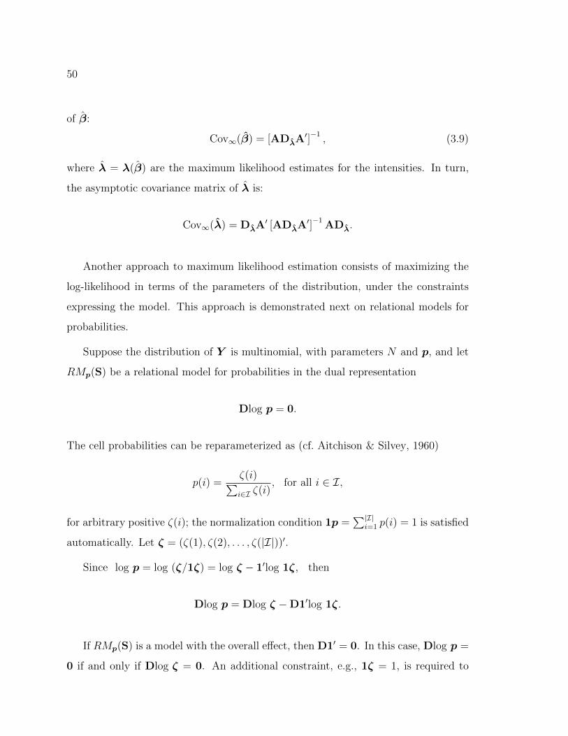
50

of β:

Cov∞(β) = [ADλA′]−1, (3.9)

where λ = λ(β) are the maximum likelihood estimates for the intensities. In turn,

the asymptotic covariance matrix of λ is:

Cov∞(λ) = DλA′ [ADλA

′]−1

ADλ.

Another approach to maximum likelihood estimation consists of maximizing the

log-likelihood in terms of the parameters of the distribution, under the constraints

expressing the model. This approach is demonstrated next on relational models for

probabilities.

Suppose the distribution of Y is multinomial, with parameters N and p, and let

RMp(S) be a relational model for probabilities in the dual representation

Dlog p = 0.

The cell probabilities can be reparameterized as (cf. Aitchison & Silvey, 1960)

p(i) =ζ(i)∑i∈I ζ(i)

, for all i ∈ I,

for arbitrary positive ζ(i); the normalization condition 1p =∑|I|

i=1 p(i) = 1 is satisfied

automatically. Let ζ = (ζ(1), ζ(2), . . . , ζ(|I|))′.

Since log p = log (ζ/1ζ) = log ζ − 1′log 1ζ, then

Dlog p = Dlog ζ −D1′log 1ζ.

If RMp(S) is a model with the overall effect, then D1′ = 0. In this case, Dlog p =

0 if and only if Dlog ζ = 0. An additional constraint, e.g., 1ζ = 1, is required to

51

ensure identifiability of ζ.

If RMp(S) is a model without the overall effect, Dlog p = 0 if and only if both

conditions, Dlog ζ = 0 and 1ζ = 1, hold. No additional identifiability constraints

are necessary in this case.

Therefore, whether or not the relational model RMp(S) has the overall effect, it

can be expressed in terms of ζ as follows:

1ζ − 1 = 0,

Dlog ζ = 0. (3.10)

The multinomial log-likelihood is equal to

l(ζ;y) = y′(log ζ − 1′log (1ζ)) + const = y′log ζ −N log (1ζ) + const.

The maximum likelihood estimate ζ exists, is unique, and can be found by maxi-

mizing the Lagrangian:

L(ζ;y) = y′log ζ −N log (1ζ) + α0(1ζ − 1) +αDlog ζ, (3.11)

where α0 and α = (α1, . . . , αK0) are the Lagrange multipliers (Aitchison & Silvey,

1958). The likelihood equations are

1

ND1/ζy −

1′

1ζ+ α01

′ + D1/ζD′α′ = 0,

1ζ − 1 = 0 (3.12)

Dlog ζ = 0.

Relational models for probabilities fit in this setup, and thus the iterative pro-

cedure for computing the maximum likelihood estimates, proposed by Aitchison &

Silvey (1958), can be used for relational models as well. To commence the itera-

52

tive process, set ζ(0) = y/N . Then, if ζ(d) stands for the dth approximation of ζ, the

(d+1)th approximation ζ(d+1) is found as the solution to the first order approximation

of the likelihood equations (3.12) in the neighborhood of ζ(d):

ζ(d+1) = ζ(d) +y

N− ζ(d)

1ζ(d)−CdHd(H

′dCdHd)

−1

H′d

[y

N− ζ(d)

1ζ(d)

]+ h(d)

. (3.13)

Here

h(d) = (1ζ(d) − 1,Dlog ζ(d))′; (3.14)

Hd = (1′,D1/ζ(d)D′);

Cd = Dζ(d) .

As d→∞, the sequence ζ(d) converges to the MLE ζ, and the matrix Pd/N , where

Pd = Cd

[I−Hd(H

′dCdHd)

−1H′dCd

], (3.15)

converges to the asymptotic covariance matrix of ζ (Aitchison & Silvey, 1960).

Both methods described in this section require matrix inversion at every step,

and the number of operations grows significantly as the number of cells in the table

increases. Modifications of each method, based on a single computation of the inverse

and thus more computationally efficient, also exist (cf. Haberman, 1974; Aitchison

& Silvey, 1958). The most recent extension of the Aitchison-Silvey algorithm was

proposed by Evans and Forcina, and they explicitly mention that their algorithm can

be used for relational models as well (Evans & Forcina, 2011, p.7).

The maximum likelihood estimates of the cell parameters can be computed using

the iterative proportional fitting procedure, which is described in detail in the next

section.

53

3.5 Iterative Proportional Fitting

Let Y be a random variable that has a distribution parameterized by δ and let y

be a realization of Y. Assume that the maximum likelihood estimate δ under a

relational model RM(S) exists and is unique. The problem of maximization of the

log-likelihood, under a relational model, can be translated into solving equations

Aδ = γb,

Dlog δ = 0, (3.16)

where γ > 0 is a known positive constant and b is a known vector with positive

components. If δ = p and RM(S) is a model for probabilities, then b = Ay/(1y),

and, if δ = λ and RM(S) is a model for intensities, then b = Ay.

In order to find a solution to the system (3.16), the following algorithm is proposed.

IPF(γ) Algorithm:

given a set of observations y; γ > 0;

set d = 0; δ(0)γ (i) = 1 for all i ∈ I; b = (b1, . . . , bJ)′, where

bj =

Ajy/(1y) if RM(S) is a model for probabilities

Ajy if RM(S) is a model for intensities, j = 1, . . . , J ;

repeat

find j ∈ 1, 2, . . . , J, such that d+ 1 ≡ j mod J ;

compute for all i ∈ I:

δ(d+1)γ (i) = δ(d)

γ (i)

(γ

bj

Ajδ(d)γ

)aji

; (3.17)

54

set d = d+ 1;

until the stopping criterion is satisfied

Here and in the sequel, A1, . . . , AJ denote the rows of the model matrix A.

The proof of convergence of IPF(γ), given below, stays valid whether or not 1 ∈

R(S) and is based on the fact that IPF(γ) is an instantiation of the algorithm proposed

by Bregman (1967) to find a common point of convex sets.

Let x,y ∈ R|I|>0 and D(x||y) denote the Bregman divergence associated with the

function F (x) =∑

i∈I x(i)log x(i):

D(x||y) =∑i∈I

x(i)log (x(i)/y(i)) + (∑i∈I

y(i)−∑i∈I

x(i)). (3.18)

If P and Q are probability distributions parameterized by p and q respectively, then

D(p||q) = I(P ||Q) is the Kullback-Leibler divergence between P and Q.

Let A1, . . . ,AJ be a family of convex sets, where Aj = z ∈ R|I|≥0 : Ajz = γbj,

for j = 1, 2, . . . , J . Since the system (3.16) is assumed consistent, the intersection of

the sets A1, . . . ,AJ is non-empty, and, for any point z in this intersection, Az = γb.

The algorithm, proposed by Bregman to find such a point, proceeds as follows:

(1) Take an arbitrary x(0) ∈ R|I|>0.

(2) For the current x(d), select an index jd(x(d)) ∈ 1, . . . , J and find x(d+1) which

is the D-projection of x(d) on the set Ajd(x(d)), that is

D(x(d+1)||x(d)) = minz∈A

jd(x(d))

D(z||x(d)) (3.19)

The sequence x(d) obtained from this process is called a relaxation sequence,

and the sequence of indices j0(x(0)), j1(x(1)), . . . is called a relaxation control. By

55

Lemma 2 (Bregman, 1967, p.202), the set of elements of any relaxation sequence x(d)

is compact and D(x(d+1)||x(d))→ 0 as d→∞.

Lemma 3.5.1. The sequence δ(d)γ , obtained from IPF(γ), is a relaxation sequence

with respect to the function D(x||y) defined in (3.18).

Proof. It will be shown first that, for every d ∈ Z≥0, δ(d+1)γ minimizes the Bregman

divergence

D(z||δ(d)γ ) =

∑i∈I

z(i)log (z(i)/δ(d)γ (i)) + (

∑i∈I

δ(d)γ (i)−

∑i∈I

z(i))

over the set Aj = z ∈ R|I|>0 : Ajz = γbj, where d+ 1 ≡ j mod J .

Let δ(d)γ be the distribution obtained during the d-th iteration, and d + 1 ≡

j mod J . Setting the derivatives of the Lagrangian

L = D(z||δ(d)γ )− α(Ajz − γbj)

=∑i∈I

z(i)log (z(i)/δ(d)γ (i)) + (

∑i∈I

δ(d)γ (i)−

∑i∈I

z(i))− α(Ajz − γbj)

equal to zero:

log (z(i)/δ(d)γ (i)) = αIj(i), i ∈ I,

Ajz = γbj.

Thus, z(i) = δ(d)γ (i) · CIj(i)

j , where

Cj =γbj

Ajδ(d)γ

.

56

Further, since aji = Ij(i), then

δ(d+1)γ (i) = δ(d)

γ (i)

[γbj

Ajδ(d)γ

]aji.

The function D(z||δ(d)γ ) is convex with respect to z, and thus it has a unique minimum

at δ(d+1)γ .

The indices in the relaxation sequence δ(d)γ are chosen in cyclic order. Bregman

(1967) showed that, for such relaxation controls, the limiting point of the relaxation

sequence is a common point of the sets Aj:

Theorem 3.5.2. (Bregman, 1967) Let the indices in a relaxation sequence x(d) be

chosen in the cyclic order, i.e.

j0(x(0)) = 1, j1(x(1)) = 2, . . . , jJ−1(x(J−1)) = J, jJ(x(J)) = 1,

and so on. Then any limiting point x∗ of the sequence x(d) is a common point of

the sets A1, . . . ,AJ .

Comment:

Compactness of a relaxation sequence implies existence of a convergent subsequence.

In the proof of Theorem 3.5.2, given by Bregman, it is shown that all convergent

subsequences converge to the same limit and, therefore, the limit of a relaxation

sequence with cyclic relaxation control exists and is unique.

The convergence of IPF(γ) is proved in the following theorem.

Theorem 3.5.3. Let Y be a random variable that has a distribution parameterized

by δ and let y be a realization of Y. Assume that the maximum likelihood estimate

δ under a relational model RM(S) exists and is unique. The sequence δ(d)γ , obtained

from IPF(γ), converges, as d→∞, and the limit δ∗γ satisfies

57

(i) Aδ∗γ = γb,

(ii) Dlog δ∗γ = 0.

Proof. (i) By Lemma 3.5.1, δ(d)γ is a relaxation sequence with respect to the func-

tion D(x||y). The indices are chosen in the cyclic order, and by Theorem 3.5.2,

the sequence δ∗γ converges and the limit is a common point of the sets A1, . . . ,AJ .

Therefore, Aδ∗γ = γb.

(ii) The argument proceeds by induction. Since δ(0)γ (i) = 1, for all i ∈ I, then

Dlog δ(0)γ = 0, and the statement holds for d = 0. Assume that Dlog δ(d)

γ = 0 for a

positive integer d. Set Cj =γbj

Ajδ(d)γ

. Then,

Dlog δ(d+1)γ = Dlog

δ

(d)γ (1) · Caj1

j

δ(d)γ (2) · Caj2

j

. . .

δ(d)γ (|I|) · Caj|I|

j

= D

log δ

(d)γ (1) + aj1log Cj

log δ(d)γ (2) + aj2log Cj

. . .

log δ(d)γ (|I|) + aj|I|log Cj

= Dlog δ(d)

γ + log CjDA′j = 0,

as D is a kernel basis matrix and thus DA′j = 0.

Therefore, by the principle of induction, Dlog δ(d)γ = 0 for all d = 0, 1, 2 . . . .

Finally, by continuity of matrix multiplication and logarithm, Dlog δ∗γ = 0.

The proof is now complete.

Corollary 3.5.4. Under the conditions of Theorem 3.5.3, the following statements

hold:

1. Let Y be a random variable that has a multinomial distribution with parameters

N and p and let y be a realization of Y. If the overall effect is present in the

58

model RMp(S), then the sequence obtained from the IPF(1) algorithm converges

to the maximum likelihood estimate p of p under the model RMp(S).

2. Let Y be a random variable that has a Poisson distribution with parameter λ and

let y be a realization of Y. Then, whether or not the overall effect is present in

the model RMλ(S), the sequence obtained from the IPF(1) algorithm converges

to the maximum likelihood estimate λ of λ under the model RMλ(S).

3. Let Y be a random variable that has a multinomial distribution with parameters

N and p and let y be a realization of Y. If the overall effect is not present in the

model RMp(S), then, if the adjustment factor γ∗ is known, the sequence obtained

from the IPF(γ∗) algorithm converges to the maximum likelihood estimate p of

p under the model RMp(S).

Proof. In the case (1), the maximum likelihood estimate p exists and satisfies the

likelihood equations

Ap = Ay/(1y),

Dlog p = 0,

which can be written in the form (3.16) with γ = 1 and b = Ay/(1y). Since p is the

unique solution, then the sequence obtained from IPF(1) converges to p.

Similarly, in the case (2), the maximum likelihood estimate λ exists and satisfies

the likelihood equations

Aλ = Ay,

Dlog λ = 0,

which can be written in the form (3.16) with γ = 1 and b = Ay. Since λ is the

59

unique solution, then the sequence obtained from IPF(1) converges to λ.

Finally, in the case (3), the maximum likelihood estimate p exists and satisfies

the likelihood equations

Ap = γ∗Ay/(1y),

Dlog p = 0,

for some γ∗ which depends on the observed distribution. The likelihood equations can

be written in the form (3.16) with γ = γ∗ and b = Ay/(1y). Since p is the unique

solution, then the sequence obtained from IPF(γ∗) converges to p.

The proof is now complete.

Table 3.2: Observed (expected) number oftrapped Charybdis japonica by bait type.

FishSugarcane Yes No

Yes 36 (35.06) 2 (2.94)No 11 (11.94) -

Table 3.3: Observed (expected) number oftrapped Portunuspelagicus by bait type.

FishSugarcane Yes No

Yes 71 (72.31) 3 (1.69)No 44 (42.69) -

Example 1.2.2 (Revisited) The model for intensities (1.5) is a regular exponential

family, and thus the maximum likelihood estimates for the cell frequencies exist and

are unique. The MLEs, shown in Tables 3.2 and 3.3, can be computed from the

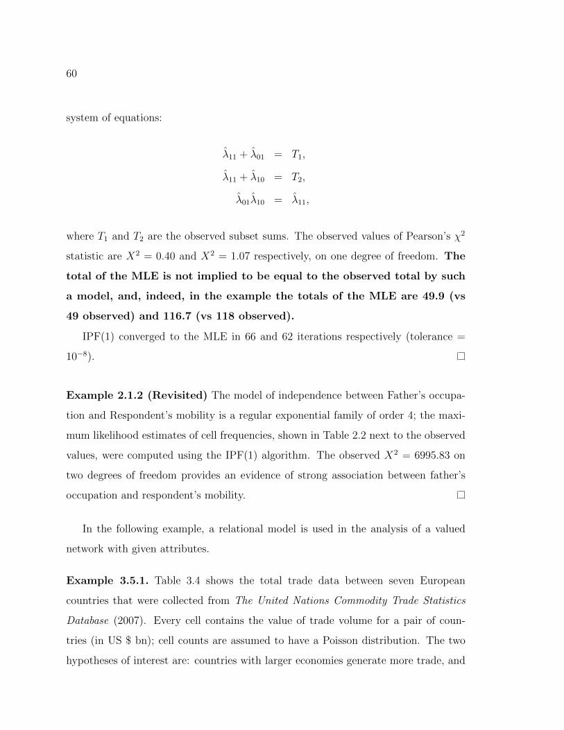
60

system of equations:

λ11 + λ01 = T1,

λ11 + λ10 = T2,

λ01λ10 = λ11,

where T1 and T2 are the observed subset sums. The observed values of Pearson’s χ2

statistic are X2 = 0.40 and X2 = 1.07 respectively, on one degree of freedom. The

total of the MLE is not implied to be equal to the observed total by such

a model, and, indeed, in the example the totals of the MLE are 49.9 (vs

49 observed) and 116.7 (vs 118 observed).

IPF(1) converged to the MLE in 66 and 62 iterations respectively (tolerance =

10−8).

Example 2.1.2 (Revisited) The model of independence between Father’s occupa-

tion and Respondent’s mobility is a regular exponential family of order 4; the maxi-

mum likelihood estimates of cell frequencies, shown in Table 2.2 next to the observed

values, were computed using the IPF(1) algorithm. The observed X2 = 6995.83 on

two degrees of freedom provides an evidence of strong association between father’s

occupation and respondent’s mobility.

In the following example, a relational model is used in the analysis of a valued

network with given attributes.

Example 3.5.1. Table 3.4 shows the total trade data between seven European

countries that were collected from The United Nations Commodity Trade Statistics

Database (2007). Every cell contains the value of trade volume for a pair of coun-

tries (in US $ bn); cell counts are assumed to have a Poisson distribution. The two

hypotheses of interest are: countries with larger economies generate more trade, and

61

trade volume between two countries is higher if they use the same currency. In this

example, GDP (gross domestic product, in US $ bn) is chosen as characterizing the

economy and Eurozone membership is chosen as the common currency indicator. The

class S includes five subsets of cells reflecting the GDP size:

GDP < 0.1 · 106 vs GDP < 0.1 · 106,

GDP < 0.1 · 106 vs 0.1 · 106 ≤ GDP < 0.6 · 106,

GDP < 0.1 · 106 vs GDP ≥ 0.6 · 106,

0.1 · 106 ≤ GDP < 0.6 · 106 vs 0.1 · 106 ≤ GDP < 0.6 · 106,

0.1 · 106 ≤ GDP < 0.6 · 106 vs GDP ≥ 0.6 · 106,

and three subsets reflecting Eurozone membership:

cells showing trade between two Eurozone members ,

cells showing trade between a Eurozone member and a non-member ,

cells showing trade between two Eurozone non-members.

Under the model generated by S, trade volume is the product of the GDP effect and

the Eurozone membership effect.

Table 3.4: Total trade between seven countries (in US $ bn). The MLEs are shownin parentheses.

LV NLD FIN EST SWE BEL LUXLV - 0.7 (3.29) 1 (1.17) 2 (2.0) 1.3 (1.17) 0.4 (1.17) 0.01 (0.01)

NLD - - 10 (17) 1 (1.17) 17 (15) 102 (102) 2.1 (2.29)FIN - - - 4 (1.17) 18 (15) 4 (2.29) 0.1 (2.29)EST - - - - 2.6 (1.17) 0.5 (1.17) 0.01 (0.01)SWE - - - - - 15 (15) 0.35 (2.29)BEL - - - - - - 9 (6.41)LUX - - - - - - -

This model is a regular exponential family of order 6. The maximum likelihood

62

estimates for cell frequencies were computed using the IPF(1) algorithm. The ob-

served X2 = 20.16 on 14 degrees of freedom yields the asymptotic p-value of 0.12; so

the model fits the trade data well. Alternatively, sensitivity of the model fit to other

choices regarding GDP could also be studied.

Since IPF(γ) is sufficient to compute the MLE under the models for intensities and

the models for probabilities with the overall effect, the algorithm described next will

only be needed for the models for probabilities without the overall effect. If 1 /∈ R(S)

and thus a relational model for probabilities RMp(S) is a curved exponential family,

then Ap = γ∗/NAy for some positive γ∗. If γ∗ is unknown, the IPF(γ) Algorithm

cannot be used to find the maximum likelihood estimates p. Complementing IPF(γ)

with a step that allows us to compute the value of γ∗ results in the algorithm that

can be used for computing the maximum likelihood estimates under relational models

for probabilities without the overall effect.

G-IPF Algorithm

given a set of observations y;

set t = 0, γ0 = 1, a step size s = s0 ∈ (0, 1]; py = y/N ;

compute δ∗γ0 using IPF(γ0)

if∑

i∈I δ∗γ0

(i) 6= 1

repeat

set γt+1 = γt − s · (∑

i∈I δ∗γt(i)− 1);

set t = t+ 1;

compute δ∗γt using IPF(γt);

until∑

i∈I δ∗γt(i) is as close to 1 as desired.

The convergence of this algorithm will be proved next.

63

Theorem 3.5.5. Let Y ∼ M(N,p), y be a realization of Y , and RMp(S) be a

relational model. For a sufficiently small step size s ∈ (0, 1], the sequence δ∗γt, obtained

from the G-IPF Algorithm, converges, as t→∞, to the maximum likelihood estimate

of p under the model RMp(S).

Proof. Suppose first that 1 ∈ R(S). The adjustment factor is initialized as γ0 = 1,

and, by Corollary 3.5.4, IPF(1) converges to the MLE of p under the model RMp(S).

Thus δ∗γ0 = p and the stopping criterion,∑∈I δ

∗γ0

(i) = 1, is satisfied.

Let now 1 /∈ R(S) and δ∗γt be the vector found using IPF(γt) on the t-th iteration.

Assume that∑

i∈I δ∗γt(i) 6= 1 and thus the convergence has not yet occurred. Consider

the next iteration of the Newton-Raphson algorithm:

δ∗γt+1

γt+1

=

δ∗γt

γt

− J−1t

Aδ∗γt − γtAp

Dlog δ∗γt

1δ∗γt − 1

.

Here Jt is the Jacobian evaluated at δ∗γt and γt. Since Aδ∗γt−γtAp = 0 and Dlog δ∗γt =

0, then γt+1 = γt−J−1t

0

0

1δ∗γt − 1

, where J−1t stands for the last row of the matrix

J−1t , and thus

γt+1 = γt − cI+1,I+1 · (∑i∈I

δ∗γt(i)− 1),

where cI+1,I+1 is the corresponding entry of the matrix J−1t . To avoid computing

cI+1,I+1, the user can replace it with a sufficiently small step size s ∈ (0, 1] that will

preserve convergence:

γt+1 = γt − s(∑i∈I

δ∗γt(i)− 1),

and then perform the iteration t + 1. The sequence γt will converge to γ∗, such that∑i∈I δ

∗γ∗(i) = 1.

64

The limiting distribution δ∗γ and the limiting value of γ∗ solve the following system

of equations:

Aδ∗γ = γ∗Ap, Dlog δ∗γ = 0, 1δ∗γ∗ = 1.

The maximum likelihood estimate p under the model RMp(S) is the unique so-

lution to this system, with γ∗ = N/α, where α is the Lagrange multiplier in (3.2).

Therefore, p = δ∗γ∗ .

The generalization of IPF proposed in this section and the computational proce-

dures described in the previous section can also be applied to models with nonnegative

integer model matrices, such as the model in Example 1.2.3.

Example 1.2.3 (Revisited) The maximum likelihood estimates for the cell frequen-

cies shown in Table 3.1 can be computed using the Newton-Raphson, Aitchison-Silvey,

and G-IPF algorithms. The approximations obtained during the first four iterations

are shown below:

Iter. Newton-Raphson Aitchison-Silvey G-IPF

1 (37.9978, 38.8930, 78.8051) (38.0736, 38.9716, 78.9549) (38.0018, 38.8955, 78.8060)

2 (38.0655, 38.9974, 78.9464) (38.0659, 38.9943, 78.9398) (38.0679, 38.9973, 78.9438)

3 (38.0634, 38.9942, 78.9421) (38.0659, 38.9943, 78.9398) (38.0659, 38.9943, 78.9396)

4 (38.0635, 38.9943, 78.9422) (38.0659, 38.9943, 78.9398) (38.0659, 38.9943, 78.9397)

G-IPF converged in 5 iterations; the Newton-Raphson algorithm converged in

5 iterations; the Aitchison-Silvey algorithm converged in 4 iterations (tolerance =

10−8).

In the next example, G-IPF is applied to a relational model which is given in

terms of generalized odds ratios.

65

Example 3.5.2. Aitchison & Silvey (1960) describe a hypothetical population in

which everyone has at least one attribute A, B, or C, and thus each individual

possesses one of the seven possible combinations of these attributes: A, B, C, AB,

BC, CA, or ABC. The structure of the population can be displayed using a 2×2×2

contingency table with one structural zero corresponding to “no attributes”. If a

random sample of N people is drawn from the population, then the number Y of

people with various combinations of the attributes is a multinomial random variable

with parameters N and p = (pA, pB, pC , pAB, pAB, pBC , pCA, pABC)′. Here pA, pB, pC ,

pAB, pAB, pBC , pCA, pABC denote positive probabilities of having the corresponding

combination of the attributes, and pA+pB +pC +pAB +pAB +pBC +pCA+pABC = 1.

The hypothesis of independence of the attributes can be stated as

pAB = pApB, pBC = pBpC , pCA = pCpA, pABC = pApBpC . (3.20)

The model expressed by (3.20) is a relational model generated by the subsets: S1

(possessing the attribute A), S2 (possessing the attribute B), and S3 (possessing the

attribute C). The model matrix and a kernel basis matrix of this model are

A =

1 0 0 1 0 1 1

0 1 0 1 1 0 1

0 0 1 0 1 1 1

, D =

1 1 0 −1 0 0 0

0 1 1 0 −1 0 0

1 0 1 0 0 −1 0

1 1 1 0 0 0 −1

;

the model is a curved exponential family of order 2.

Let y = (46, 24, 7, 15, 3, 4, 1) be a realization of Y. Then the maximum likelihood

estimates of y under the model (3.20) are approximately

y = (46.90, 26.27, 7.82, 12.32, 2.06, 3.67, 0.96).

66

The estimates were obtained by all three algorithms: the G-IPF algorithm converged

in 6 iterations, and both the Newton-Raphson algorithm and the Aitchison-Silvey

algorithm converged in 5 iterations (tolerance = 10−8).

A summary of the properties of the MLE under relational models is given in Table

3.5.

Table 3.5: Relational models and properties of the MLE.

Models for probabilities Models for intensitiesOverall effect Overall effectPresent Not present Present Not present

Subset Sums of theMLE vs observedsubset sums

Equal Proportional Equal Equal

Total of the MLE vsobserved total

Equal Equal Equal Not equal

Exponential family Regular Curved Regular RegularIPF version IPF(1) G-IPF IPF(1) IPF(1)

The computer code implementing the algorithms described in this section and in

Section 3.4 is provided in the Appendix. The IPF(1) algorithm will be employed for

computing the maximum likelihood estimates under the models for social mobility

proposed in the next chapter.

67

Chapter 4

COORDINATE FREE COMPARATIVE ANALYSIS OFSOCIAL MOBILITY

Introduction

In this chapter, the relational model framework will be used for analysis of trends

in social mobility. Greater social mobility is usually considered advantageous for a

society, and results of analyses comparing the patterns and trends of social mobility

across years or between different nations are often given a political interpretation.

This work intends to contribute to the debate about declining social mobility in

Great Britain (cf. Saunders, 2010).

If a society is stratified according to some criteria, then every individual can be

assigned to one and only one stratum. The strata are often referred to as social

classes or statuses. Social mobility is a transition of an individual from one social

position to another (Sorokin, 1964). Intergenerational social mobility is a change of

social position of an individual (son), as compared to that of his origin (father). A

detailed account of social mobility research was given by Ganzeboom et al. (1991)

and Treiman & Ganzeboom (2000).

A social mobility table is a cross-classification of individuals according to their

own and their father’s social status. Let I be the total number of social classes in the

stratification of interest, F and S be random variables, taking values in 1, 2, . . . , I

and indicating Father’s (Origin) and Son’s (Destination) status respectively. A social

68

mobility table can be written as an I × I contingency table:

Destination

1 2 . . . I

Ori

gin

1 p11 p12 . . . p1I

2 p21 p21 . . . p2I

......

.... . .

...

I pI1 pI2 . . . pII

(4.1)

where pij ∈ (0, 1), for all i, j = 1, . . . , I,∑I

i,j=1 pij = 1, and pij is the proportion of

sons in class j whose fathers were in class i.

A social mobility table does not include a variable characterizing mobility per se,

and mobility trends are usually inferred from the marginals and the association struc-

ture of the table. The marginal distributions reveal changes in the social structure

that occurred between the fathers’ and sons’ generations, and the part of mobility,

that can be attributed to those changes, is called structural or “forced” mobility. The

component of mobility that is not structural is referred to as exchange mobility. Ab-

solute mobility is the proportion of sons whose status is different from that of their

fathers:

g =∑i 6=j

pij.

If the statuses are ordered, e.g., from the most prestigious to the least prestigious,

every individual is identified as upward (downward) mobile, i.e., having a higher

(lower) status than his father, or immobile, i.e., retaining his father’s status. The

concept of horizontal mobility is used to reflect changes in status that cannot be

considered as advantageous (upward) or disadvantageous (downward) (cf. Sorokin,

1964; Goldthorpe & Jackson, 2007).

Absolute mobility is also characterized by outflow rates, computed from the con-

69

ditional distribution of Son’s status given Father’s status:

pijpi+

, for i, j = 1, . . . , I.

Outflow rates are usually compared with the marginal distribution of Son’s status

that shows which opportunities sons have, independent of their father’s position.

Relative mobility was defined by Glass (1954) as “the different opportunities of

gaining high status available to individuals of different social origin”. Relative mobil-

ity is described by the association structure of the table, and relative mobility rates

are equal to odds ratiospiipjjpjipij

=pii/pijpji/pjj

.

Thus, relative rates indicate the chances of an individual from class i to stay in this

class rather than move to class j, relative to the chances of an individual from class

j to move to class i rather than stay in class j (cf. Goldthorpe & Jackson, 2007).

A weaker association between the social position of an individual and his origin,

called higher social fluidity, implies higher chances of mobility. Equality of chances

of movement for individuals of all social statuses, called “perfect mobility”, means

independence of Father’s and Son’s status:

pij = pi+p+j, for i, j = 1, . . . , I.

The expected values of the cell frequencies, under perfect mobility, are used in various

mobility indices that measure social mobility in terms of the departure of observed mo-

bility from perfect mobility (see, Glass (1954), Bibby (1975), Boudon (1973), among

others).

The model of perfect mobility expresses the hypothesis of no association between

Father’s status and Son’s status, and under this model the log cell probabilities in

70

the mobility table can be written in the log-linear representation of

log pij = λ+ λFi + λSj , (4.2)

where λFi and λSj are effects associated with Father’s status and with Son’s status, re-

spectively. (Here and in the sequel, the model parameters are subject to appropriate

identifiability constraints.) This model does not fit most data sets, because few soci-

eties are perfectly mobile. Models of “quasi-perfect mobility” that take into account

the possibility of status inheritance were proposed by White (1963) and Goodman

(1965). One such model, the model of quasi-independence (Goodman, 1968), entirely

removes restrictions from the diagonal cells by allowing for additional parameters:

log pij = λ+ λFi + λSj + δiI(i = j), i, j = 1, . . . , I, (4.3)

where

I(i = j) =

1 if i = j

0 otherwise.,

and the parameters δi characterize the departure of the diagonal cells from indepen-

dence. A general approach to modeling a specific pattern of association in mobility

tables with ordinal categories was also developed by Goodman (1969, 1972).

In order to account for an arbitrary pattern of association in a mobility table

with unordered categories, Hauser (1978) proposed a structural model, which is also

called a levels model or a topological model (Hout, 1983). The levels H1, H2, . . . , HL

are a partition of the cells in a mobility table, and, under the model, the log cell

probabilities are sums of the effects associated with Father’s and Son’s statuses and

the interaction effects, that are assumed to be identical for all cells that belong to the

same level:

log pij = λ+ λFi + λSj +L∑l=1

Il(i, j)δl. (4.4)

71

Here

Il(i, j) =

1 if the cell(i, j) ∈ Hl

0 otherwise,

and δl, for l = 1, . . . , L, are level specific parameters. Each parameter “reflects the

level of mobility or immobility in that cell relative to that in other cells in the table”

(Hauser, 1978). The levels are determined empirically, and their number should be

substantially less than the number of cells in the table (Hauser, 1978, 1980). Clogg

& Shockey (1984) suggested that cells belonging to the same level have to share some

common substantive property. In turn, Kovach, Robert, & Rudas (1986) considered

levels consisting of contiguous cells.

Models which accounted for the social distance between Fathers’ and Sons’ sta-

tuses, as if it was measured on the interval scale, were proposed, among others, by

Goodman (1972), Sobel (1981), Hope (1982), Agresti (1983), Hauser (1984). These

models assume that the distance between categories i1 and i2 is the same as between

categories i3 and i4 (1 ≤ i1, i2, i3, i4 ≤ I), if |i1 − i2| = |i3 − i4|.

Comparative mobility research concentrates on revealing changes in social mobility

between different cohorts, e.g., across years or between countries, and aims to compare

absolute and relative mobility rates in several social mobility tables that have the same

categories for origin and destination:

Destination

Cohort 1 1 2 . . . I

Ori

gin

1 p111 p121 . . . p1I1

2 p211 p211 . . . p2I1

......

.... . .

...

I pI11 pI21 . . . pII1

, . . . ,

Destination

Cohort K 1 2 . . . I

Ori

gin

1 p11K p12K . . . p1IK

2 p21K p21K . . . p2IK

......

.... . .

...

I pI1K pI2K . . . pIIK

.

Here pijk ∈ (0, 1), for all i, j = 1, . . . , I, k = 1, . . . , K, and∑I

i,j=1

∑Kk=1 pijk = 1.

72

Without loss of generality, it will be assumed in the sequel that the cohorts correspond

to different years.

The baseline model for comparative analysis is the model of conditional inde-

pendence of Father’s and Son’s status given Year (Y ) that assumes that there is no

association between Father’s and Son’s status within each year:

log pijk = λ+ λFi + λSj + λYk + λFYik + λSYjk . (4.5)

Under the model of common (or constant) social fluidity (CSF), see Hauser et al.

(1975), Erikson & Goldthorpe (1992), the association between Father’s and Son’s

status is allowed to exist and be different in every cell, but is assumed to be identical

for each year (no second order association between F , S, and Y ):

log pijk = λ+ λFi + λSj + λYk + λFYik + λSYjk + λFSij . (4.6)

If, instead of the λFSij term, Hauser’s levels are allowed, a constant pattern of fluidity

model (Erikson et al., 1982) is obtained. The model (4.6) says that marginal distri-

butions of Father’s and Son’s status change across years, but the association between

them does not.

Several generalizations of this model were proposed to allow the association be-

tween Father’s status and Son’s Status to vary over time. Yamaguchi (1987) intro-

duced the uniform layer effect model, under which the pattern of association changes

uniformly across years:

log pijk = λ+ λFi + λSj + λYk + λFYik + λSYjk + λFSij + ijβk + δijDFYik , (4.7)

where δij is Kronecker’s delta, DFYik are status-specific diagonal effects, and the sta-

tuses are assumed to be ordered from high to low on the interval scale. Here βk is the

relative strength of the F×S association in year k, and∑K

k=1 βk = 0. If βk is negative

73

(positive), then the association between Father’s status and Son’s Status in the year

k is uniformly smaller (larger) than the average association for all tables included in

the analysis.

Another generalization of (4.6) is the UNIDIFF (uniform difference) model (Erik-

son & Goldthorpe, 1992), also called the log-multiplicative layer effect model (Xie,

1992). This model allows for more flexibility in specifying the association between

Father’s status and Son’s Status:

log pijk = λ+ λFi + λSj + λYk + λFYik + λSYjk + ψijφk. (4.8)

Under the model, the F × S × Y association is separated into the F × S and Y

components. The pattern of the F × S association, expressed by the parameters ψij,

is assumed to be the same across years, but the relative strength of this association,

expressed by the parameters φk, can differ for k = 1, . . . , K. Depending on the con-

straints placed on the parameters ψij and φk, this model can be a reparameterization

of the CSF model or can lead to some other models for mobility tables (Xie, 1992). A

UNIDIFF model is used to test whether the odds ratios in the kth year are uniformly

higher or uniformly lower than the odds ratios in the reference year. However, this

is an assumption that may or may not hold in practice: there are cases where the

pattern of mobility does not change as specified by a UNIDIFF model (cf. Wong,

1994).

The association structure of the table, operationalized as various sets of odds

ratios, reflects the chances of individuals who come from different positions to end up

in different social statuses. Although much of social mobility research is concerned

with the analysis of the association structure of social mobility tables (cf. Goodman &

Hout, 1998; Breen, 2008), neither the marginals nor the association structure quantify

social mobility itself, and the question, as to where is social mobility present in the

mobility table, persists.

74

The methods that will be described in Section 4.2 are based on the observation

that social mobility is a common characteristic of some of the cells of the mobility

table. For example, if mobility is only considered as being upward or downward,

then, if statuses are ordered from highest to lowest, upward mobility is a common

characteristic of cells (and observations) in the lower diagonal triangle, downward

mobility is a common characteristic of the upper diagonal triangle, and the cells on

the main diagonal are characterized by immobility. If social status is considered

to have many categories, then mobility can be categorized by the number of steps

up or down from the father’s position, forming mobility bands parallel to the main

diagonal. The models proposed in this work include effects associated with these

bands of mobility. Since the mobility effects are not based on any of the variables

forming the table, the models are coordinate free.

4.1 Data and Previous Analyses

The analysis in this chapter is based on the two data sets that were also analyzed in

“Trends in intergenerational class mobility in modern Britain: evidence from national

surveys, 1972–2005” (Goldthorpe & Mills, 2008), referred to as TICM in the sequel,

and “Is social mobility really declining? Intergenerational class mobility in Britain in

the 1990s and the 2000s” (Li & Devine, 2011), referred to as SMD. Both TICM and

SMD relied on the 1991 British Household Panel Survey (BHPS-91) and the 2005

General Household Survey (GHS-05). The mobility tables used by TICM and SMD

are based on the seven-class analytic version of the National Statistics Socio-economic

Classification (NS-SEC): 1. Higher managerial and professional occupations; 2. Lower

managerial and professional occupations; 3. Intermediate occupations; 4. Small em-

ployers and own account workers; 5. Lower supervisory and technical occupations;

6. Semi-routine occupations; 7. Routine occupations.

The NS-SEC, introduced in 2001, is an instantiation of the Goldthorpe class

schema (Erikson & Goldthorpe, 1992) and is now used for all official statistics and

75

surveys in the United Kingdom. The NS-SEC category of an individual is derived

from the full employment information, which, in addition to the occupation, contains

data on whether an individual is an employer, self-employed or an employee, whether

or not he is a supervisor, and data on the workplace size. The NS-SEC category of a

household is determined by the NS-SEC category of the Household Reference Person

(cf. Rose & Pevalin, 2003). In the British Household Panel Survey, the household

reference person is defined as the person who is legally or financially responsible for

the family accommodation or the elder person of those equally responsible (Institute

for Social & Economic Research, 2011b). In the 2005 General Household Survey, the

household reference person is the person with the highest income or the elder of two

if they have exactly the same income (Economic and Social Data Service, 2011a).

The BHPS-91 is the first wave of the British Household Panel Survey (Institute

for Social & Economic Research, 2011a). The BHPS-91 sample consists of 10,264

individuals from 5,505 households, among whom 97 percent (9912 respondents) had

full interviews; response rate to individual interview was 92.2 percent (out of 10751

eligible adults, there were 426 refusals and 46 non-contacts) (Institute for Social &

Economic Research, 2011c). The survey collects the full information on the respon-

dents’ employment status and that of their parents. Respondents’ occupational status

is determined as their current main job, parental occupational statuses are determined

as father’s and mother’s jobs when the respondent was 14.

The GHS (Economic and Social Data Service, 2011b) has been held since 1971

and, up to 2004, had a cross-sectional design. Starting from 2005, when the GHS was

chosen to include the British component for the European Union Statistics on Income

and Living Conditions Survey, its sampling design was changed to longitudinal and

the information on parental occupational status has been again collected (it was not

in 1993-2004). The GHS-05 sample consists of 30,069 people from 16,778 households,

among whom 72 percent gave a full interview, and the overall response rate was 74

percent.

76

Since the GHS collects information on parental occupation only for respondents

older than 25, TICM included in their analyses respondents between 25 and 59 years

old. The total number of male respondents in this age group with valid occupational

statuses both for themselves and their parents in the two data sets was found to be

6435 (Goldthorpe & Mills, 2008). Following a dominance approach (Erikson, 1984),

Li & Devine (2011) chose the family origin class as the highest of father’s and mother’s

class and thus found 6595 male respondents with a valid occupational status of origin

and destination in the 25-59 age group.

Although the authors of SMD aimed to reproduce and expand the analyses de-

scribed in TICM for the two surveys, they used somewhat different procedures to

derive the NS-SEC from the survey data. The GSH collects only partial employ-

ment information on parents (their occupation), and TICM derived the class origin

from occupational data alone, following the procedure proposed by ONS (Office for

National Statistics, 2011). In order to increase comparability of the 1991 and 2005

social mobility tables, TICM followed the same procedure for the respondent’s origin

class in the BHPS-91 and did not use the full employment information on parental

class that was available. SMD did use the full employment information given in the

BHPS data and found the NS-SEC for both respondent’s and parental classes as rec-

ommended by Rose & Pevalin (2003). In the case of the GHS-05, SMD proposed their

own procedure: first, they match-coded the SOC and the NS-SEC for respondent’s

class and, then, used the match to derive the NS-SEC for parental class (Li & Devine,

2011, p.13).

Due to different definitions of the origin class and different coding procedures, the

mobility tables derived in TICM and in SMD are not the same. Consequently, the

fit statistics, shown in Table 4.1, as well as some of the results in TICM and SMD

do not completely agree. For example, while TICM reports almost identical rates

of upward mobility for men in 1991 and 2005, SMD detects a significant decrease in

upward mobility and a significant increase in downward mobility for men. Despite

77

the differences, both papers conclude that association between Fathers’ and Sons’

positions was decreasing, which means that social fluidity for men was increasing and

the society was becoming more open.

Table 4.1: Fit statistics and p-values.

Goldthorpe & Mills (2008) Li & Devine (2011)

Model df G2 p-value G2 p-value

Cond Ind 72 756.9 0.00 652.8 0.00

CSF 36 19.3 0.99 51.3 0.00

UNIDIFF 35 15.5 0.99 34.5 0.49

The percentage data obtained in SMD for male respondents of age 25-59, trans-

formed to frequencies and given in Table 4.2, are used for the analysis in this chapter.

4.2 Relational Models of Social Mobility

Two relational models for the comparative analysis of mobility tables will be described

in this section. The model (4.5) of conditional independence of Father’s and Son’s

status given Year will be used as the baseline model. This model assumes that, within

a given year, Father and Son effects are independent from each other and thus the

relative rates of mobility are equal to 1. Since this model doesn’t fit the data (see

Table 4.1), further, mobility-related, effects will be included.

The relational models are generated by the cylinder sets associated with the F×Y

effect and S × Y effect and by the subsets, called mobility bands. A mobility band is

a collection of those cells that represent the same number and direction of steps from

Father’s position to Son’s position within each year. Each diagonal cell has its own

effect, so that model fit is not influenced by immobile cells.

78

Table 4.2: Distribution of men by class of origin and destination.

Destination1991 1 2 3 4 5 6 7

Ori

gin

1 50 47 5 11 11 5 82 124 166 24 61 55 29 473 37 50 8 18 24 13 214 61 66 13 97 50 21 535 71 113 24 74 100 74 1036 34 71 11 50 69 74 957 40 79 18 71 105 74 105

Destination2005 1 2 3 4 5 6 7

Ori

gin

1 182 139 28 32 28 24 482 246 297 51 123 91 87 1273 67 95 12 36 40 24 404 55 79 12 63 55 51 595 99 139 28 75 87 75 1036 75 115 12 75 95 91 1197 67 119 16 79 91 79 135

Under the model called Mdiff,

log pijk = λ0 + λFi + λSj + λYk + λFYik + λSYjk +38∑h=1

βhIUh(i, j, k), (4.9)

for i, j = 1, . . . , 7, k = 1, 2. Here IUh , for each h = 1, . . . , 38, is the indicator function

of the mobility band Uh. The mobility bands Uh are shown in Table 4.3; cells belonging

to the same band are marked with the same number.

Under the model Mdiff, the mobility effects are allowed to be different for the two

years. The fit of this model will be compared to that of the model Msame. Under

the model Msame, the mobility effects are supposed to be the same for the two years.

The definition of the mobility bands Vh is given in Table 4.4, and the model can be

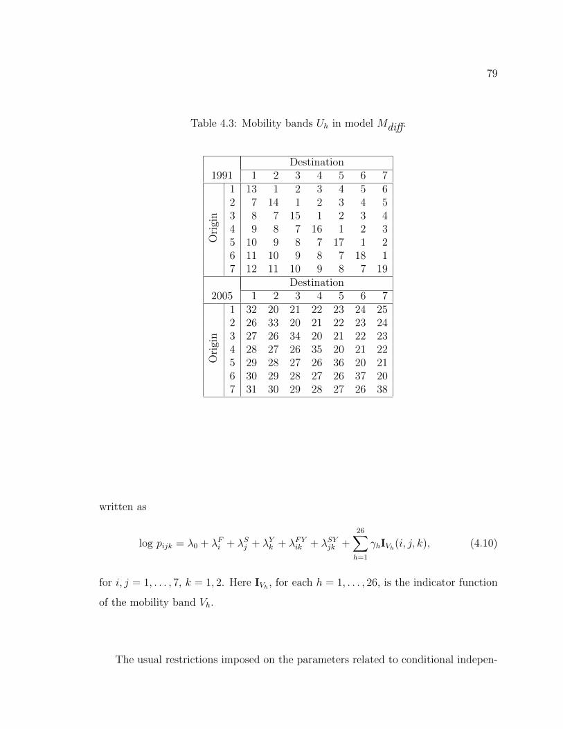
79

Table 4.3: Mobility bands Uh in model Mdiff.

Destination1991 1 2 3 4 5 6 7

Ori

gin

1 13 1 2 3 4 5 62 7 14 1 2 3 4 53 8 7 15 1 2 3 44 9 8 7 16 1 2 35 10 9 8 7 17 1 26 11 10 9 8 7 18 17 12 11 10 9 8 7 19

Destination2005 1 2 3 4 5 6 7

Ori

gin

1 32 20 21 22 23 24 252 26 33 20 21 22 23 243 27 26 34 20 21 22 234 28 27 26 35 20 21 225 29 28 27 26 36 20 216 30 29 28 27 26 37 207 31 30 29 28 27 26 38

written as

log pijk = λ0 + λFi + λSj + λYk + λFYik + λSYjk +26∑h=1

γhIVh(i, j, k), (4.10)

for i, j = 1, . . . , 7, k = 1, 2. Here IVh , for each h = 1, . . . , 26, is the indicator function

of the mobility band Vh.

The usual restrictions imposed on the parameters related to conditional indepen-

80

Table 4.4: Mobility bands Vh in model Msame.

Destination1991 1 2 3 4 5 6 7

Ori

gin

1 13 1 2 3 4 5 62 7 14 1 2 3 4 53 8 7 15 1 2 3 44 9 8 7 16 1 2 35 10 9 8 7 17 1 26 11 10 9 8 7 18 17 12 11 10 9 8 7 19

Destination2005 1 2 3 4 5 6 7

Ori

gin

1 20 1 2 3 4 5 62 7 21 1 2 3 4 53 8 7 22 1 2 3 44 9 8 7 23 1 2 35 10 9 8 7 24 1 26 11 10 9 8 7 25 17 12 11 10 9 8 7 26

dence

7∑i=1

λFi = 0,7∑j=1

λSj = 0,2∑

k=1

λYk = 0,

2∑k=1

λFYik = 0,2∑

k=1

λSYjk = 0, for i, j = 1, . . . , 7; (4.11)

7∑i=1

λFYik = 0,7∑j=1

λSYjk = 0, for k = 1, 2,

do not suffice to make all parameters of the models identifiable, and more constraints

are needed. The band parameters associated with upward and with downward mo-

bility are thus centered around 1 on the multiplicative scale within both years for the

81

model Mdiff:

6∑h=1

βh = 0,12∑h=7

βh = 0,25∑

h=20

βh = 0,31∑

h=26

βh = 0, (4.12)

and are centered around 1 on the multiplicative scale for the model Msame:

6∑h=1

γh = 0,12∑h=7

γh = 0.

Both models include the overall effect, expressed by the parameter λ0, and, by

Theorem 2.3.2, are regular exponential families. By Theorem 3.2.1, the maximum

likelihood estimates of cell frequencies under these models can be computed using the

IPF(1) algorithm described in Section 3.5.

The data used in this analysis were assembled from two independent surveys,

and thus product-multinomial sampling is a better approximation of reality than

multinomial sampling. Asymptotic standard errors for log-linear models under the

product-multinomial sampling scheme were obtained by Lang (1996). He used the

derivation techniques originally proposed by Aitchison & Silvey (1958) and discussed

earlier in Chapter 3, Section 3.4. If A and D stand, respectively, for the model matrix

and a kernel basis matrix, then the asymptotic covariance matrix of the parameters

of the model is equal to (Lang, 1996, Eq.(4.5))

Cov∞(β) = (AA′)−1ACov∞(f)A′(AA′)−1. (4.13)

The asymptotic covariance matrix of the cell frequencies equals (Lang, 1996, Eq.(4.6))

Cov∞(f) = Df −D′(D(Df )−1D′)−1D−

f 1f′1/N1 O

O f 2f′2/N2

(4.14)

Here N1 = 2630 and N2 = 3965 are the numbers of respondents in 1991 and in 2005,

82

respectively.

4.3 Results

The fit statistics and p-values for the models Msame and Mdiff are given in Table 4.5.

The model Msame does not fit well and, thus, the data provide some evidence that

the pattern of mobility changed between the two timepoints. Parameter estimates

from the model Mdiff will be used to describe these changes.

Table 4.5: Relational models: fit statistics and p-values.

Model df G2 p-value

Mdiff 38 45.18 0.19

Msame 48 66.94 0.04

The maximum likelihood estimates, under the model Mdiff, for the mobility effects

(on the multiplicative scale), their ratios, and the applicable standard errors are shown

in Table 4.6 1. The effects are centered around 1 on both sides of the main diagonal by

assumption (4.12). The standard errors for the mobility effects were computed from

(4.13), and the standard errors for the ratios were obtained using the delta method.

The estimated mobility effects for both years versus the number of steps up or

down from the origin are displayed in Figure 4.1. The plot indicates that mobility

decreases monotonically as the number of steps from the origin increases. Therefore,

moving a small number of steps up or down from the origin seems to be easier than

making larger steps. For 1991, the effects depend very little on direction and the plot

is almost symmetric, less so in 2005. In 2005, small moves (1-3 steps) appear to be

less likely than in 1991, and for 5 out of these 6 levels the changes are statistically

1Parameter estimation for relational models that contain the overall effect, like Mdiff, can be

performed using the gnm() function in the R package.

83

Table 4.6: Estimated mobility effects (under product multinomial sampling) for themodel Mdiff.

Distance from the origin 1991 2005 Ratio6 steps down 0.44 (0.13) 0.78 (0.10) 1.77 (0.56)

5 steps down 0.69 (0.10) 0.79 (0.06) 1.14 (0.19)

4 steps down 0.93 (0.12) 0.86 (0.07) 0.92 (0.14)

3 steps down 1.25 (0.13) 0.93 (0.07) 0.74 (0.09)

2 steps down 1.46 (0.13) 1.35(0.08) 0.92 (0.10)

1 step down 1.92 (0.14) 1.49 (0.08) 0.78 (0.07)

1 step up 1.78 (0.11) 1.45 (0.07) 0.81 (0.06)

2 steps up 1.57 (0.11) 1.30 (0.08) 0.83 (0.07)

3 steps up 1.33 (0.09) 1.10 (0.07) 0.83 (0.08)

4 steps up 1.01 (0.08) 0.97 (0.07) 0.96 (0.10)

5 steps up 0.66 (0.06) 0.82 (0.06) 1.24 (0.15)

6 steps up 0.41 (0.06) 0.60 (0.07) 1.46 (0.27)

significant at the 95% level. For 4 steps of mobility, the chances in the two years are

nearly identical. Large moves (5-6 steps) appear to be slightly more likely in 2005 than

in 1991, which implies more openness for the British society in 2005. Although the

increase was not found statistically significant (see Table 4.6), the lack of significance

does not occur due to smaller estimated effect sizes for increased chances of more steps

of mobility in 2005 compared to 1991, rather because of larger estimated standard

errors for these quantities.

The analyses based on the relational models offer a number of advantages in

comparative mobility research. The proposed models allow for mobility effects that

are not associated with variables or groups of variables in the table. An F × S

interaction is not assumed beyond the one associated with having made a certain

number of steps up or down, and a finer analysis of the changing mobility patterns

84

0.5

1.0

1.5

Number of Steps from the Origin

Est

imat

ed M

obili

ty E

ffect

−6 −5 −4 −3 −2 −1 1 2 3 4 5 6

1991 effects2005 effects

Figure 4.1: Estimated mobility effects under Mdiff.

is possible. The mobility effect in the model Mdiff is not assumed to be linear or

other parametric function of F and S and is therefore modeled in a semi-parametric

way. This makes it possible to analyze different numbers and directions of steps

independently of each other, revealing effects when change is statistically significant

for some levels but not significant for others.

Relational models retain the flexibility of Hauser’s topological models, but the

coordinate-free nature makes it simpler to add additional attributes to the analyses,

for example, grandparents’ or siblings’ social statuses. Finally, the semi-parametric

approach based on the relational models can be applied to modeling structure or

change in structure in other areas, including biology or social networks.

85

Appendix A

MAXIMUM LIKELIHOOD ESTIMATION USING R

A.1 The Newton-Raphson Method: Models for Intensities

The supplementary R-function p.beta computes the cell parameters of a distribution

from a relational model. The function has two arguments: ModelMatrix - a model

matrix of full row rank, beta - a vector of log-linear parameters. The function returns

a vector of the cell parameters corresponding to the values of log-linear parameters

given.

The R-function Newton.intens computes the maximum likelihood estimates un-

der a relational model for intensities, using the Newton-Raphson algorithm described

in Section 3.4. The function has three arguments: ModelMatrix - a model ma-

trix of full row rank, ObsTable - a vector of observed cell counts, tol - a toler-

ance (precision), equal to a very small positive real number. The function returns

subset.parameters - the maximum likelihood estimates of the log-linear parame-

ters associated with the subsets in the generating class, SE.subset.parameters -

standard errors for those parameters, fitted.values - the maximum likelihood es-

timates for the cell intensities under the model, SE.fitted.values - standard er-

rors for the estimates of the cell intensities, method - the type of relational model

("intensities"), degrees.of.freedom - the number of degrees of freedom of the

model, chisq.statistic - Pearson’s χ2 statistic, p.value - the p-value, iterations

- the number of iterations until convergence.

> library(dlm)

> p.beta <- function(ModelMatrix, beta)

+ A <- ModelMatrix

86

+ N <- ncol(A)

+ J <- nrow(A)

+ if (J != length(beta))

+ stop("Dimensions of the model matrix and of the vector of

+ parameters do not match")

+ s <- numeric(N)

+ for (i in 1:N)

+ s[i] <- exp(A[, i] %*% beta)

+

+ return(s)

+

> Newton.intens <- function(ModelMatrix, ObsTable, tol)

+ A <- ModelMatrix

+ y <- ObsTable

+ N <- length(y)

+ J <- nrow(A)

+ if (N != ncol(A))

+ stop("Dimensions of the model matrix and

+ the data vector do not match")

+ if (J != (qr(A)$rank))

+ stop("The model matrix is not full row rank")

+ param_0 <- rep(1, J)

+ JMi <- A %*% bdiag(p.beta(A, param_0)) %*% t(A)

+ param_1 <- param_0 - solve(JMi) %*% (A %*% p.beta(A, param_0) -

+ A %*% y)

+ nit <- 0

+ while (sqrt(sum((param_0 - param_1)^2)) > tol)

+ param_0 <- param_1

+ covar_0 <- solve(A %*% bdiag(p.beta(A, param_0)) %*%

+ t(A))

+ param_1 <- param_0 - covar_0 %*% (A %*% p.beta(A, param_0) -

+ A %*% y)

+ nit <- nit + 1

+

+ mleTable <- p.beta(A, param_1)

+ SE_par <- numeric(J)

+ for (j in 1:J)

+ SE_par[j] <- sqrt(covar_0[j, j])

+

+ Cov_intens <- bdiag(mleTable) %*% t(A) %*% covar_0 %*% A %*%

87

+ bdiag(mleTable)

+ SE_intens <- numeric(N)

+ for (j in 1:N)

+ SE_intens[j] <- sqrt(Cov_intens[j, j])

+

+ chisqv <- sum((ObsTable - mleTable)^2/mleTable)

+ df <- N - J

+ pv <- 1 - pchisq(chisqv, df)

+ result <- list(subset.parameters = param_1[1:J],

+ SE.subset.parameters = SE_par,

+ fitted.values = mleTable,

+ SE.fitted.values = SE_intens,

+ method = "intensities",

+ degrees.of.freedom = df,

+ chisq.statistic = chisqv,

+ p.value = pv,

+ iterations = nit)

+ return(result)

+

A.2 The Aitchison-Silvey Method: Models for Probabilities

The supplementary R-function se.prob computes the standard errors, as per Aitchi-

son & Silvey (1958) for the maximum likelihood estimates of the cell frequencies under

a relational model for probabilities, see Section 3.4. The function has two arguments:

KernelBasis - a kernel basis matrix of full row rank, mleTable - a vector of the

MLEs. The function returns a vector of standard errors for the estimates of the MLE

of the cell frequencies.

The R-function AS.prob computes the maximum likelihood estimates under a

relational model for probabilities, using the Aitchison-Silvey algorithm described in

Section 3.4. The function has three arguments: KernelBasis - a kernel basis ma-

trix of full row rank, ObsTable - a vector of observed cell counts, tol - a toler-

ance (precision), equal to a very small positive real number. The function returns

fitted.values - the maximum likelihood estimates for the cell frequencies under the

88

model, SE.fitted.values - standard errors for the estimates of the cell frequencies,

method - the type of relational model ("probabilities"), degrees.of.freedom - the

number of degrees of freedom of the model, chisq.statistic - Pearson’s χ2 statistic,

p.value - the p-value, iterations - the number of iterations until convergence.

> library(dlm)

> se.prob <- function(KernelBasis, mleTable)

+ D <- KernelBasis

+ if (nrow(D) != (qr(KernelBasis)$rank))

+ stop("The kernel basis matrix is not full row rank")

+ total <- sum(mleTable)

+ mle_p <- mleTable/total

+ N <- length(mle_p)

+ one <- rep(1, N)

+ H <- t(rbind(one, D %*% bdiag(1/mle_p)))

+ Bi <- bdiag(mle_p)

+ P <- (total) * Bi %*% (bdiag(one) - H %*% solve(t(H) %*%

+ Bi %*% H) %*% t(H) %*% Bi)

+ SE <- numeric(N)

+ for (i in 1:N) SE[i] <- sqrt(P[i, i])

+ return(SE)

+

> AS.prob <- function(KernelBasis, ObsTable, tol)

+ N <- sum(ObsTable)

+ I <- length(ObsTable)

+ if (I != ncol(KernelBasis))

+ stop("Dimensions of the kernel basis matrix and

+ the data vector do not match")

+ if (nrow(KernelBasis) != (qr(KernelBasis)$rank))

+ stop("The kernel basis matrix is not full row rank")

+ zeta0 <- ObsTable/N

+ Bi <- bdiag(zeta0)

+ Hi <- t(rbind(rep(1, length(zeta0)), KernelBasis %*% bdiag(1/zeta0)))

+ li <- 1/sum(ObsTable) * bdiag(1/zeta0) %*% ObsTable - rep(1/sum(zeta0),

+ length(zeta0))

+ hi <- rbind(sum(zeta0) - 1, KernelBasis %*% log(zeta0))

+ zeta1 <- zeta0 + Bi %*% li - Bi %*% Hi %*% solve(t(Hi) %*%

+ Bi %*% Hi) %*% (t(Hi) %*% Bi %*% li + hi)

+ nit <- 0

89

+ while (sqrt(sum((zeta0 - zeta1)^2)) > tol)

+ zeta0 <- zeta1

+ Bi <- bdiag(zeta0)

+ Hi <- t(rbind(rep(1, length(zeta0)), KernelBasis %*%

+ bdiag(1/zeta0)))

+ li <- 1/sum(ObsTable) * bdiag(1/zeta0) %*% ObsTable -

+ rep(1/sum(zeta0), length(zeta0))

+ hi <- rbind(sum(zeta0) - 1, KernelBasis %*% log(zeta0))

+ zeta1 <- zeta0 + Bi %*% li - Bi %*% Hi %*% solve(t(Hi) %*%

+ Bi %*% Hi) %*% (t(Hi) %*% Bi %*% li + hi)

+ nit <- nit + 1

+

+ mleTable <- N * t(zeta1)

+ SE <- se.prob(KernelBasis, mleTable)

+ chisqv <- sum((ObsTable - mleTable)^2/mleTable)

+ df <- nrow(KernelBasis)

+ pv <- 1 - pchisq(chisqv, df)

+ result <- list(fitted.values = mleTable,

+ SE.fitted.values = SE,

+ method = "probabilities",

+ degrees.of.freedom = df,

+ chisq.statistic = chisqv,

+ p.value = pv,

+ iterations = nit)

+ return(result)

+

A.3 Generalized Iterative Proportional Fitting

The R-function ipf.gamma computes the maximum likelihood estimates under a rela-

tional model, using the IPF(γ) algorithm described in Section 3.5. The function has

the following arguments: ModelMatrix - a model matrix of full row rank, ObsTable

- a vector of observed cell counts, gamma - the adjustment factor, tol - a tolerance

(precision), equal to a very small positive real number, method - the type of relational

model ("probabilities" or "intensities"). The function returns the maximum

likelihood estimates for the cell frequencies under the model.

90

The R-function g.ipf computes the maximum likelihood estimates under a rela-

tional model for probabilities, using the G-IPF algorithm described in Section 3.5.

The function has following arguments: ModelMatrix - a model matrix of full row

rank, ObsTable - a vector of observed cell counts, tol - a tolerance (precision), equal

to a very small positive real number, step - a positive number not exceeding 1 for the

adjustment step. The function returns adjustment.factor - the adjustment factor

for the observed table, fitted.values - maximum likelihood estimates for the cell

frequencies under the model, degrees.of.freedom - the number of degrees of free-

dom of the model, chisq.statistic - Pearson’s χ2 statistic, p.value - the p-value,

iterations - the number of iterations until convergence.

> ipf.gamma <- function(ModelMatrix, ObsTable, gamma, tol, method)

+ nr <- nrow(ModelMatrix)

+ nc <- ncol(ModelMatrix)

+ if (length(ObsTable) != nc)

+ stop("Dimensions of the model matrix and of

+ the data vector do not match")

+ Total <- sum(ObsTable)

+ m1 <- rep(1, nc)

+ m2 <- m1

+ m3 <- m2

+ SuffStat <- rep(0, nr)

+ if (method == "probabilities")

+ for (h in 1:nr)

+ SuffStat[h] <- (ObsTable/Total) %*% ModelMatrix[h,

+ ]

+

+

+ if (method == "intensities")

+ for (h in 1:nr)

+ SuffStat[h] <- (ObsTable) %*% ModelMatrix[h, ]

+

+

+ for (j in 1:nr)

+ for (i in 1:nc)

+ m2[i] <- m1[i] * (gamma * SuffStat[j]/(m1 %*% ModelMatrix[j,

+ ]))^(ModelMatrix[j, i])

91

+

+ m1 <- m2

+

+ while (sum((m3 - m2)^2) > tol)

+ m3 <- m2

+ m1 <- m2

+ for (j in 1:nr)

+ for (i in 1:nc)

+ m2[i] <- m1[i] * (gamma * SuffStat[j]/(m1 %*%

+ ModelMatrix[j, ]))^(ModelMatrix[j, i])

+

+ m1 <- m2

+

+

+ return(m2)

+

> g.ipf <- function(ModelMatrix, ObsTable, tol, step)

+ nc = ncol(ModelMatrix)

+ if (length(ObsTable) != nc)

+ stop("Dimensions of the model matrix and of

+ the data vector do not match")

+ gamma <- 1

+ p <- ipf.gamma(ModelMatrix, ObsTable, gamma, tol, "probabilities")

+ Total <- sum(p)

+ k <- 0

+ if (abs(Total - 1) > tol)

+ k <- 1

+ while (abs(Total - 1) > tol)

+ gamma <- gamma - step * (Total - 1)

+ p <- ipf.gamma(ModelMatrix, ObsTable, gamma, tol,

+ "probabilities")

+ Total <- sum(p)

+ k <- k + 1

+

+

+ mleTable <- sum(ObsTable) * p

+ chisqv <- sum((ObsTable - mleTable)^2/mleTable)

+ df <- nc - qr(ModelMatrix)$rank

+ pv <- 1 - pchisq(chisqv, df)

+ result <- list(adjustment.factor = gamma,

92

+ fitted.values = mleTable,

+ degrees.of.freedom = df,

+ chisq.statistic = chisqv,

+ p.value = pv,

+ iterations = k - 1)

+ return(result)

+

A.4 Computation of a Kernel Basis Matrix

The R-function kernel.basis returns an integer basis for the kernel of the given

matrix ModelMatrix. An intuitive algorithm is implemented: the transpose of the

given model matrix is augmented by the identity matrix of the appropriate size, and

then the Gauss method is used to find the reduced echelon form of the augmented

matrix.

> kernel.basis <- function(ModelMatrix)

+ subsets <- nrow(ModelMatrix)

+ nvar <- ncol(ModelMatrix)

+ M1 <- cbind(t(ModelMatrix), diag(rep(1, nvar)))

+ rows <- nvar

+ cols <- rows + subsets

+ rows1 <- nrow(M1)

+ cols1 <- ncol(M1)

+ c_col <- 1

+ rank <- 0

+ i <- 1

+ epsilon <- 1e-06 ## since integers are represented

+ ## by real numbers, precision is needed

+ while ((i <= rows1) && (c_col <= cols1))

+ k <- i

+ ndx <- -1

+ for (k in i:rows1)

+ aVal <- abs(M1[k, c_col])

+ if (aVal > epsilon)

+ ndx <- k

+ break

93

+

+

+ if (ndx > -1)

+ lead <- M1[ndx, c_col]

+ for (j in c_col:cols1)

+ temp <- M1[ndx, j]/lead

+ if (i != ndx)

+ M1[ndx, j] <- M1[i, j]

+ M1[i, j] <- temp

+

+

+ diag <- M1[i, c_col]

+ if (diag != 0)

+ for (m in 1:rows1)

+ if (m != i)

+ f <- M1[m, c_col]/diag

+ if (f != 0)

+ for (q in c_col:cols1)

+ M1[m, q] <- M1[m, q] - M1[i, q] * f

+ if (abs(M1[m, q]) < epsilon)

+ M1[m, q] <- 0

+

+

+

+ rank <- rank + 1

+ i <- i + 1

+

+ c_col <- c_col + 1

+

+ degf <- 0

+ for (row in 1:rows)

+ count <- sum(abs(M1[row, 1:subsets]))

+ if (count == 0)

+ degf <- degf + 1

+

+ C <- M1[(rows - degf + 1):rows, (subsets + 1):cols]

+ return(C)

+

94

Appendix B

EXAMPLES

B.1 Bait Study for Swimming Crabs

Kawamura et al. (1995) showed that sugarcane-fish combination was more effective

than fish for trapping swimming crabs. In this work, the model for intensities express-

ing the multiplicative effect of using two bait types at the same time is tested, see

Example 1.2.2. This model is a regular exponential family, and the maximum likeli-

hood estimates for intensities under this model can be computed using the functions

Newton.intens or ipf.gamma. The R-output is given below:

> A <- matrix(c(1, 1, 0, 1, 0, 1), 2, 3, byrow = T)

> y1 <- c(36, 2, 11)

> y2 <- c(71, 3, 44)

> Newton.intens(A, y1, 1e-08)

$subset.parameters

[1] 1.077475 2.479664

$SE.subset.parameters

[1] 0.2905868 0.2612875

$fitted.values

[1] 35.062746 2.937254 11.937254

$SE.fitted.values

[1] 5.7318409 0.8535271 3.1190557

$method

[1] "intensities"

$degrees.of.freedom

[1] 1

95

$chisq.statistic

[1] 0.3977122

$p.value

[1] 0.5282732

$iterations

[1] 7

> Newton.intens(A, y2, 1e-08)

$subset.parameters

[1] 0.5268632 3.7540493

$SE.subset.parameters

[1] 0.1871948 0.1501622

$fitted.values

[1] 72.306389 1.693611 42.693611

$SE.fitted.values

[1] 8.4091194 0.3170353 6.4109681

$method

[1] "intensities"

$degrees.of.freedom

[1] 1

$chisq.statistic

[1] 1.071277

$p.value

[1] 0.3006572

$iterations

[1] 15

> ipf.gamma(A, y1, 1, 1e-08, method = "intensities")

96

[1] 35.062854 2.937289 11.937146

> ipf.gamma(A, y2, 1, 1e-08, method = "intensities")

[1] 72.306475 1.693617 42.693525

B.2 Pneumonia Infection in Calves

Agresti (2002) describes a study carried out to determine if a pneumonia infection

has an immunizing effect on dairy calves. The model of no immunizing effect of

the pneumonia infection is considered in Example 1.2.3. This model is a curved

exponential family, the maximum likelihood estimates for probabilities under this

model can be computed using the functions AS.prob or g.ipf. The R-output is

shown below:

> A = matrix(c(2, 1, 0, 0, 1, 1), 2, 3, byrow = T)

> y = c(30, 63, 63)

> g.ipf(A, y, 1e-08, 1)

$adjustment.factor

[1] 0.936004

$fitted.values

[1] 38.06350 38.99431 78.94219

$degrees.of.freedom

[1] 1

$chisq.statistic

[1] 19.70608

$p.value

[1] 9.031362e-06

$iterations

[1] 5

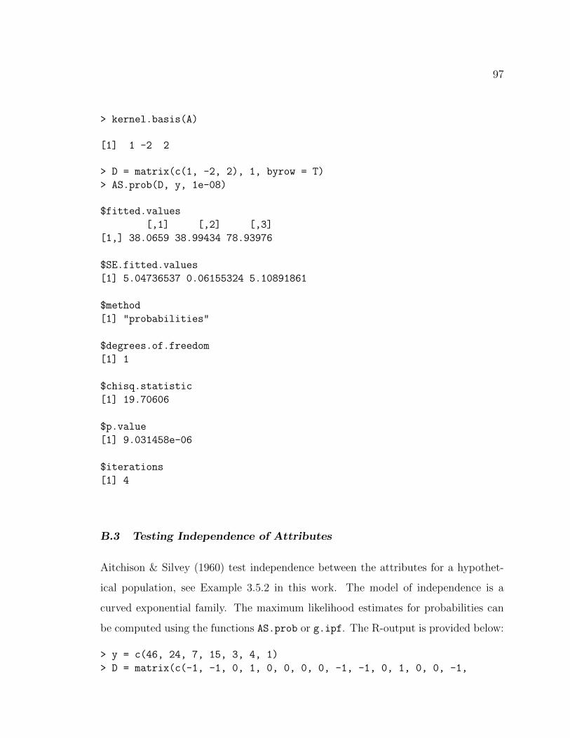
97

> kernel.basis(A)

[1] 1 -2 2

> D = matrix(c(1, -2, 2), 1, byrow = T)

> AS.prob(D, y, 1e-08)

$fitted.values

[,1] [,2] [,3]

[1,] 38.0659 38.99434 78.93976

$SE.fitted.values

[1] 5.04736537 0.06155324 5.10891861

$method

[1] "probabilities"

$degrees.of.freedom

[1] 1

$chisq.statistic

[1] 19.70606

$p.value

[1] 9.031458e-06

$iterations

[1] 4

B.3 Testing Independence of Attributes

Aitchison & Silvey (1960) test independence between the attributes for a hypothet-

ical population, see Example 3.5.2 in this work. The model of independence is a

curved exponential family. The maximum likelihood estimates for probabilities can

be computed using the functions AS.prob or g.ipf. The R-output is provided below:

> y = c(46, 24, 7, 15, 3, 4, 1)

> D = matrix(c(-1, -1, 0, 1, 0, 0, 0, 0, -1, -1, 0, 1, 0, 0, -1,

98

+ 0, -1, 0, 0, 1, 0, -1, -1, -1, 0, 0, 0, 1), byrow = T, ncol = 7)

> AS.prob(D, y, 1e-08)

$fitted.values

[,1] [,2] [,3] [,4] [,5] [,6] [,7]

[1,] 46.90312 26.26506 7.82409 12.31913 2.055002 3.669742 0.9638599

$SE.fitted.values

[1] 4.6153343 3.7612937 2.0270154 1.0517339 0.5468675 0.8780194 0.1879930

$method

[1] "probabilities"

$degrees.of.freedom

[1] 4

$chisq.statistic

[1] 1.348567

$p.value

[1] 0.8530833

$iterations

[1] 4

> A = matrix(c(1, 0, 0, 1, 0, 1, 1, 0, 1, 0, 1, 1, 0, 1, 0, 0,

+ 1, 0, 1, 1, 1), byrow = T, nrow = 3)

> g.ipf(A, y, 1e-08, 1)

$adjustment.factor

[1] 0.967513

$fitted.values

[1] 46.9030842 26.2650859 7.8240907 12.3191354 2.0550042 3.6697399

[7] 0.9638603

$degrees.of.freedom

[1] 4

$chisq.statistic

[1] 1.348566

99

$p.value

[1] 0.8530834

$iterations

[1] 6

100

REFERENCES

Agresti, A. (1983). A simple diagonals-parameter symmetry and quasi-symmetry

model. Statist. Probab. Lett., 1 , 313–316.

Agresti, A. (2002). Categorical data analysis. New York: Wiley.

Aitchison, J., & Silvey, S. D. (1958). Maximum-likelihood estimation of parameters

subject to restraints. The Annals of Mathematical Statistics , 29 , 813–828.

Aitchison, J., & Silvey, S. D. (1960). Maximum-likelihood estimation procedures and

associated tests of significance. J. Roy. Statist. Soc. Ser.B , 22 , 154–171.

Andersen, A. H. (1974). Multidimensional contingency tables. Scand. J. Statist., 1 ,

115–127.

Barndorff-Nielsen, O. E. (1976). Factorization of likelihood functions for full expo-

nential families. J. Roy. Statist. Soc. Ser.B , 38 , 37–44.

Barndorff-Nielsen, O. E. (1978). Information and exponential families. New York:

Wiley.

Bergsma, W., & Rudas, T. (2003). On conditional and marginal association. Ann.

Fac. Sci. Toulouse, 11 , 455–468.

Bertsekas, D. P. (2009). Convex optimization theory. Nashua, NH: Athena Scientific.

Bibby, J. (1975). Methods of measuring mobility. Quality & Quantity , 9 , 107–136.

Birch, M. W. (1963). Maximum likelihood in three-way contingency tables. J. Roy.

Statist. Soc. Ser.B , 25 , 220–233.

101

Bishop, Y. M. M., Fienberg, S. E., & Holland, P. W. (1975). Discrete multivariate

analysis: theory and practice. MIT.

Blau, P. M., & Duncan, O. D. (1967). The American occupational structure. New

York: John Wiley and Sons, Inc.

Boudon, R. (1973). Mathematical structures of social mobility. San-Francisco, CA:

Jossey-Bass Inc., Publishers.

Breen, R. (2008). Statistical models of association for comparing cross-classification.

Sociol.Methods Res., 36 , 442–461.

Bregman, L. M. (1967). The relaxation method of finding the common point of

convex sets and its application to the solution of problems in convex programming.

U.S.S.R. Computational Mathematics and Mathematical Physics , 7 (3), 200–217.

Brown, L. D. (1988). Fundamentals of statistical exponential families. Hayward,

Calif.: Institute of Mathematical Statistics.

Casella, G., & Berger, R. L. (2002). Statistical inference. Pacific Grove, Calif.:

Duxbury.

Christensen, R. (1997). Log-linear models and logistic regression. New York: Springer.

Clogg, C. C., & Shockey, J. W. (1984). A note on two models for mobility tables.

Comparative Social Research, 7 , 443–462.

Csiszar, I. (1975). I-divergence geometry of probability distributions and minimization

problems. Ann. Probab., 3 , 146–158.

Darroch, J. N., & Ratcliff, D. (1972). Generalized iterative scaling for log-linear

models. The Annals of Mathematical Statistics , 43 , 1470–1480.

102

Diaconis, P., & Sturmfels, B. (1998). Algebraic methods for sampling from conditional

distributions. Ann. Statist., 26 , 363–397.

Drton, M., Sturmfels, B., & Sullivant, S. (2009). Lectures on algebraic statistics

(Vol. 39). Birkhauser Verlag AG.

Economic and Social Data Service. (2011a). General Household Survey 2005: Def-

initions and Terms. Appendix A. Available from http://www.esds.ac.uk/doc/

6265/mrdoc/pdf/appendixa.pdf (last accessed on December 3, 2011)

Economic and Social Data Service. (2011b). General Lifestyle Survey. Available

from http://www.esds.ac.uk/government/ghs/ (last accessed on November 23,

2011)

Efron, B. (1975). Defining the curvature of a statistical problem (with applications

to second order efficiency). Ann. Statist., 3 , 1189–1242.

Erikson, R. (1984). Social class of men, women and families. Sociology , 18 , 500–514.

Erikson, R., & Goldthorpe, J. H. (1992). The constant flux. Clarendon Press, Oxford.

Erikson, R., Goldthorpe, J. H., & Portocarero, L. (1982). Social fluidity in industrial

nations: England, France and Sweden. The British Journal of Sociology , 33 , 1–34.

Evans, R. J., & Forcina, A. (2011). Two algorithms for fitting constrained marginal

models. arXiv: 1110.2894v1.

Fienberg, S. E. (1970). An iterative procedure for estimation in contingency tables.

The Annals of Mathematical Statistics , 41 , 907–917.

Ganzeboom, H. B. G., Treiman, D. J., & Ultee, W. C. (1991). Comparative intergen-

erational stratification research: three generations and beyond. Annu. Rev. Sociol.,

17 , 277–302.

103

Glass, D. B. (1954). Social mobility in Britain. London: Routledge and Kegan Paul.

Goldthorpe, J. H., & Jackson, M. (2007). Intergenerational class mobility in con-

temporary Britain: political concerns and empirical findings. British Journal of

Sociology , 58 , 525–546.

Goldthorpe, J. H., & Mills, C. (2008). Trends in intergenerational class mobility

in modern Britain: evidence from national surveys, 1972–2005. National Institute

Economic Review , 205 , 83–100.

Goodman, L. A. (1965). On the statistical analysis of mobility tables. American

Journal of Sociology , 70 , 564–585.

Goodman, L. A. (1968). The analysis of cross-classified data: independence, quasi-

independence, and interaction in contingency tables with or without missing cells.

J. Amer. Statist. Assoc., 63 , 1091–1131.

Goodman, L. A. (1969). How to ransack social mobility tables and other kinds of

cross-classification tables. American Journal of Sociology , 75 , 1–39.

Goodman, L. A. (1972). Some multiplicative models for the analysis of cross-classified

data. Proceedings of the Sixth Berkley Symposium on Mathematical Statistics and

Probability , 649–696.

Goodman, L. A., & Hout, M. (1998). Statistical methods and graphical displays for

analyzing how the association between two qualitative variables differs among coun-

tries, among groups, or over time: a modified regression-type approach. Sociological

Methodology , 28 , 175–230.

Haberman, S. J. (1974). The analysis of frequency data (Vol. IV). The University of

Chicago Press.

104

Hauser, R. M. (1978). A structural model of the mobility table. Social Forces , 56 ,

919–953.

Hauser, R. M. (1980). Some exploratory methods for modelling mobility tables and

other cross-classified data. Sociological Methodology , 11 , 413–458.

Hauser, R. M. (1984). Vertical class mobility in England, France, and Sweden. Acta

Sociologica, 27 , 87–110.

Hauser, R. M., Koffel, J. H., & Dickinson, P. J. (1975). Temporal change in occu-

pational mobility: evidence for men in the United States. Am. Sociol. Rev., 40 ,

279–297.

Hoffmann-Jørgensen, J. (1994). Probability with a view toward statistics (Vol. 2).

New York: Chapman & Hall.

Hope, K. (1982). Vertical and nonvertical class mobility in three countries. Am.

Sociol. Rev., 47 , 99–113.

Hout, M. (1983). Mobility tables (Vol. 31). Sage Publications, Inc.

Hubbard, J. H., & Hubbard, B. B. (1999). Vector calculus, linear algebra, and

differential forms: a unified approach. New Jersey, USA: Prentice Hall.

Institute for Social & Economic Research. (2011a). British Household Panel Survey.

Available from http://www.iser.essex.ac.uk/bhps (last accessed on November

19, 2011)

Institute for Social & Economic Research. (2011b). British Household Panel Survey.

FAQs. Households. Available from http://www.iser.essex.ac.uk/bhps/faqs/

households (last accessed on December 3, 2011)

Institute for Social & Economic Research. (2011c). Quality profile: British House-

hold Panel Survey. Available from http://www.iser.essex.ac.uk/files/bhps/

105

quality-profiles/BHPS-QP-01-03-06-v2.pdf (last accessed on December 3,

2011)

Kass, R. E., & Vos, P. W. (1997). Geometrical foundations of asymptotic inference.

New York: Wiley.

Kawamura, G., Matsuoka, T., Tajiri, T., Nishida, M., & Hayashi, M. (1995). Ef-

fectiveness of a sugarcane-fish combination as bait in trapping swimming crabs.

Fisheries Research, 22 , 155–160.

Klimova, A., & Rudas, T. (2012). Coordinate free analysis of trends in British social

mobility. J. Appl. Stat..

Klimova, A., Rudas, T., & Dobra, A. (2012). Relational models for contingency

tables. J. Multivariate Anal., 104 , 159–173.

Kovach, I., Robert, P., & Rudas, T. (1986). Towards the dimensions of mobility.

in Andorka, R., Bertalan, L.(eds.) Economy and Society in Hungary, Budapest ,

153–183.

Lang, J. B. (1996). On the comparison of multinomial and Poisson log-linear models.

J. Roy. Statist. Soc. Ser.B , 58 , 253–266.

Li, Y., & Devine, F. (2011). Is social mobility really declining? Intergenerational

class mobility in Britain in the 1990s and the 2000s. Sociological Research Online,

16 .

Office for National Statistics. (2011). Derivation tables. Available from http://

www.ons.gov.uk/ons/index.html (last accessed on November 15, 2011)

Pachter, L., & Sturmfels, B. (Eds.). (2005). Algebraic statistic for computational

biology. Cambridge University Press.

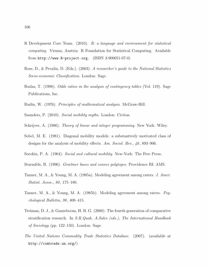
106

R Development Core Team. (2010). R: a language and environment for statistical

computing. Vienna, Austria: R Foundation for Statistical Computing. Available

from http://www.R-project.org. (ISBN 3-900051-07-0)

Rose, D., & Pevalin, D. (Eds.). (2003). A researcher’s guide to the National Statistics

Socio-economic Classification. London: Sage.

Rudas, T. (1998). Odds ratios in the analysis of contingency tables (Vol. 119). Sage

Publications, Inc.

Rudin, W. (1976). Principles of mathematical analysis. McGraw-Hill.

Saunders, P. (2010). Social mobility myths. London: Civitas.

Schrijver, A. (1986). Theory of linear and integer programming. New York: Wiley.

Sobel, M. E. (1981). Diagonal mobility models: a substantively motivated class of

designs for the analysis of mobility effects. Am. Sociol. Rev., 46 , 893–906.

Sorokin, P. A. (1964). Social and cultural mobility. New-York: The Free Press.

Sturmfels, B. (1996). Groebner bases and convex polytopes. Providence RI: AMS.

Tanner, M. A., & Young, M. A. (1985a). Modeling agreement among raters. J. Amer.

Statist. Assoc., 80 , 175–180.

Tanner, M. A., & Young, M. A. (1985b). Modeling agreement among raters. Psy-

chological Bulletin, 98 , 408–415.

Treiman, D. J., & Ganzeboom, H. B. G. (2000). The fourth generation of comparative

stratification research. In S.R.Quah, A.Sales (eds.), The International Handbook

of Sociology (pp. 122–150). London: Sage.

The United Nations Commodity Trade Statistics Database. (2007). (available at

http://comtrade.un.org/)

107

White, H. C. (1963). Cause and effect in social mobility tables. Behavioral Science,

8 , 14–27.

Wong, R. S. (1994). Postwar mobility trends in advanced industrial societies. Research

in Social Stratification and Mobility , 13 , 121–144.

Xie, Y. (1992). The log-multiplicative layer effect model for comparing mobility

tables. Am. Sociol. Rev., 57 , 380–395.

Yamaguchi, K. (1987). Models for comparing mobility tables: toward parsimony and

substance. Am. Sociol. Rev., 52 , 482–494.

Young, M. A., Tanner, M. A., & Meltzer, H. Y. (1982). Operational definitions

of schizophrenia: What do they identify? The Journal of Nervous and Mental

Disease, 170 , 443–447.

108

VITA

Anna Klimova was born in Leningrad, U.S.S.R. In 1993, she earned a Candidate of

Sciences degree in Mathematics at Saint-Petersburg State University. Her thesis was

supervised by Professor Vasilii Babich. From 1992 to 2000, Anna taught Mathematics

at the University of Telecommunications in Saint-Petersburg. She joined the Statistics

Department at the University of Washington in September 2007. In April 2012 she

became a Doctor of Philosophy.