13
DERIVADAS PARCIAIS Seção 14.3
© 2003 Brooks/Cole, a division of Thomson Learning, Inc.
Thomson Learning™ is a trademark used herein under license.
2
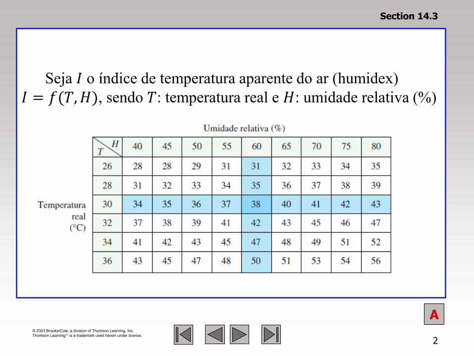
Seja 𝐼 o índice de temperatura aparente do ar (humidex)
𝐼 = 𝑓(𝑇, 𝐻), sendo 𝑇: temperatura real e 𝐻: umidade relativa (%)
Digite a equação aqui.
Section 14.3
A

© 2003 Brooks/Cole, a division of Thomson Learning, Inc.
Thomson Learning™ is a trademark used herein under license.
3
Seja 𝑓 uma função de duas variáveis 𝑥 e 𝑦. Tomemos no ponto 𝑎, 𝑏
E consideramos a seguinte situação:
𝑥 é variável e 𝑦 = 𝑏 𝑓𝑖𝑥𝑜
𝑓𝑥 𝑎, 𝑏 = limℎ→0
𝑓 𝑎 + ℎ, 𝑏 − 𝑓(𝑎, 𝑏)
ℎ
, se o limite existir.
Section 14.2
A

© 2003 Brooks/Cole, a division of Thomson Learning, Inc.
Thomson Learning™ is a trademark used herein under license.
4
𝑦 é variável e x = a (𝑓𝑖𝑥𝑜)
𝑓𝑦 𝑎, 𝑏 = limℎ→0
𝑓 𝑎, 𝑏 + ℎ − 𝑓(𝑎, 𝑏)
ℎ
, se o limite existir.
Section 14.2
A

© 2003 Brooks/Cole, a division of Thomson Learning, Inc.
Thomson Learning™ is a trademark used herein under license.
5
Seja 𝑓 uma função de duas variáveis 𝑥 e 𝑦, suas derivadas parciais
são:
Derivada Parcial em relação a 𝒙:
𝜕𝑓(𝑥, 𝑦)
𝜕𝑥= 𝑓𝑥 𝑥, 𝑦 = lim
ℎ→0
𝑓 𝑥 + ℎ, 𝑦 − 𝑓(𝑥, 𝑦)
ℎ
Derivada Parcial em relação a y:
𝜕𝑓(𝑥, 𝑦)
𝜕𝑦= 𝑓𝑦 𝑥, 𝑦 = lim
ℎ→0
𝑓 𝑥, 𝑦 + ℎ − 𝑓(𝑥, 𝑦)
ℎ
, se os limites existirem.
Exemplo: Seja 𝑓 𝑥, 𝑦 = 3𝑥2𝑦 . Use a definição de derivadas parciais
para determinar 𝜕𝑓(1,2)
𝜕𝑥 e
𝜕𝑓(1,2)
𝜕𝑦
Section 14.3
A

© 2003 Brooks/Cole, a division of Thomson Learning, Inc.
Thomson Learning™ is a trademark used herein under license.
6
NOTAÇÕES:
𝑓𝑥 𝑥, 𝑦 = 𝑓𝑥 =𝜕𝑓(𝑥, 𝑦)
𝜕𝑥=
𝜕𝑓
𝜕𝑥= 𝐷𝑥𝑓
𝑓𝑦 𝑥, 𝑦 = 𝑓𝑦 =𝜕𝑓(𝑥, 𝑦)
𝜕𝑦=
𝜕𝑓
𝜕𝑦= 𝐷𝑦𝑓
Técnica para determinar as derivadas parciais de 𝑧 = 𝑓(𝑥, 𝑦)
1. Para determinar 𝑓𝑥 𝑥, 𝑦 , trate 𝑦 como uma constante e derive 𝑓 𝑥, 𝑦
em relação a 𝒙.
2. Para determinar 𝑓𝑦 𝑥, 𝑦 , trate x como uma constante
e derive 𝑓 𝑥, 𝑦 em relação a y.
.
Section 14.3
A

© 2003 Brooks/Cole, a division of Thomson Learning, Inc.
Thomson Learning™ is a trademark used herein under license.
7
Sendo a superfície 𝑆 o gráfico da função 𝑧 = 𝑓 𝑥, 𝑦 ,um ponto
𝑃 𝑎, 𝑏, 𝑐 ∈ 𝑆, isto é, f 𝑎, 𝑏 = 𝑐 , 𝐶1 o corte de 𝑆 quando 𝑦 = 𝑏
e 𝐶2 o corte de 𝑆 quando 𝑥 = 𝑎.
Section 14.3 Figures 2, 3
Interpretação geométrica das derivadas parciais

© 2003 Brooks/Cole, a division of Thomson Learning, Inc.
Thomson Learning™ is a trademark used herein under license.
8
As derivadas parciais 𝑓𝑥(𝑎, 𝑏) e 𝑓𝑦(𝑎, 𝑏) podem ser geometrica-
mente como as inclinações das retas tangentes em 𝑃 aos cortes 𝐶1 𝑒 𝐶2
de 𝑆, respectivamente.
Ou ainda,
• 𝑓𝑥(𝑥, 𝑦) é igual a taxa de variação 𝜕𝑧
𝜕𝑥 em relação a 𝑥
quando 𝑦 é mantido fixo.
• 𝑓𝑦(𝑥, 𝑦) é igual a taxa de variação 𝜕𝑧
𝜕𝑦 em relação a 𝑦
quando x é mantido fixo.
Section 14.3
Interpretação geométrica das derivadas parciais

© 2003 Brooks/Cole, a division of Thomson Learning, Inc.
Thomson Learning™ is a trademark used herein under license.
9
Derivadas Parciais

© 2003 Brooks/Cole, a division of Thomson Learning, Inc.
Thomson Learning™ is a trademark used herein under license.
10
Exemplo 1: Determine as derivadas parciais da função
𝑓 𝑥, 𝑦 = 5𝑥3 − 5𝑥3𝑦2
Exemplo 2: Seja 𝑓 𝑥, 𝑦 = 4 − 𝑥2 − 2𝑦2. Determine 𝑓𝑥(1,1) e 𝑓𝑦(1,1) e interprete esses números como
inclinações.
Propostos: Determine as derivadas parciais a seguir:
a) 𝑧 = 𝑓 𝑥, 𝑦 = 𝑥2 + 𝑦2
b) 𝑧 = 𝑓 𝑥, 𝑦 = 𝑥2 + 𝑦2 cos(𝑥𝑦) no ponto 1, 𝜋
c) f 𝑥, 𝑦) = ln (𝑥2 + 𝑦2
d) g 𝑥, 𝑦 = 𝑎𝑟𝑐 𝑡𝑔 (𝑥
𝑦)
e) 𝑓 𝑥, 𝑦, 𝑧 = exylnz

© 2003 Brooks/Cole, a division of Thomson Learning, Inc.
Thomson Learning™ is a trademark used herein under license.
11
Seja 𝑓(𝑥, 𝑦, 𝑧), a derivada parcial em relação à 𝑥 é definida como
𝜕𝑓(𝑥, 𝑦, 𝑧)
𝜕𝑥= lim
ℎ→0
𝑓 𝑥 + ℎ, 𝑦, 𝑧 − 𝑓(𝑥, 𝑦, 𝑧)
ℎ
Funções de 𝑛 Variáveis Seja 𝑢 = f(x1, x2, … , xn) a sua derivada parcial em relação a
𝑖 −ésima variável 𝑥𝑖 é:
𝜕𝑢
𝜕𝑥𝑖= lim
ℎ→0
𝑓 𝑥1, 𝑥2, … . , 𝑥𝑖 + ℎ, … , 𝑥𝑛 − 𝑓(𝑥1, 𝑥2, … . , 𝑥𝑖 , … , 𝑥𝑛)
ℎ
* Considerando que os limites existam.
Section 14.3
A
Funções de Três Variáveis

© 2003 Brooks/Cole, a division of Thomson Learning, Inc.
Thomson Learning™ is a trademark used herein under license.
12
- Derivadas Parciais de segunda ordem:
𝒇𝒙 𝒙 = 𝒇𝒙𝒙 = 𝜕
𝜕𝑥
𝜕𝑓
𝜕𝑥=
𝜕2𝑓
𝜕𝑥2
𝒇𝒚 𝒚= 𝒇𝒚𝒚 =
𝜕
𝜕𝑦
𝜕𝑓
𝜕𝑦=
𝜕2𝑓
𝜕𝑦2
𝒇𝒙 𝒚 = 𝒇𝒙𝒚 = 𝜕
𝜕𝑦
𝜕𝑓
𝜕𝑥=
𝜕2𝑓
𝜕𝑦𝜕𝑥
Section 14.3
A
- Derivadas Parciais de ordem superior
𝒇𝒙𝒚𝒚 = 𝒇𝒙𝒚 𝒚=
𝜕
𝜕𝑦
𝜕2𝑓
𝜕𝑦𝜕𝑥=
𝜕3𝑓
𝜕𝑦2𝜕𝑥
© 2003 Brooks/Cole, a division of Thomson Learning, Inc.
Thomson Learning™ is a trademark used herein under license.
13
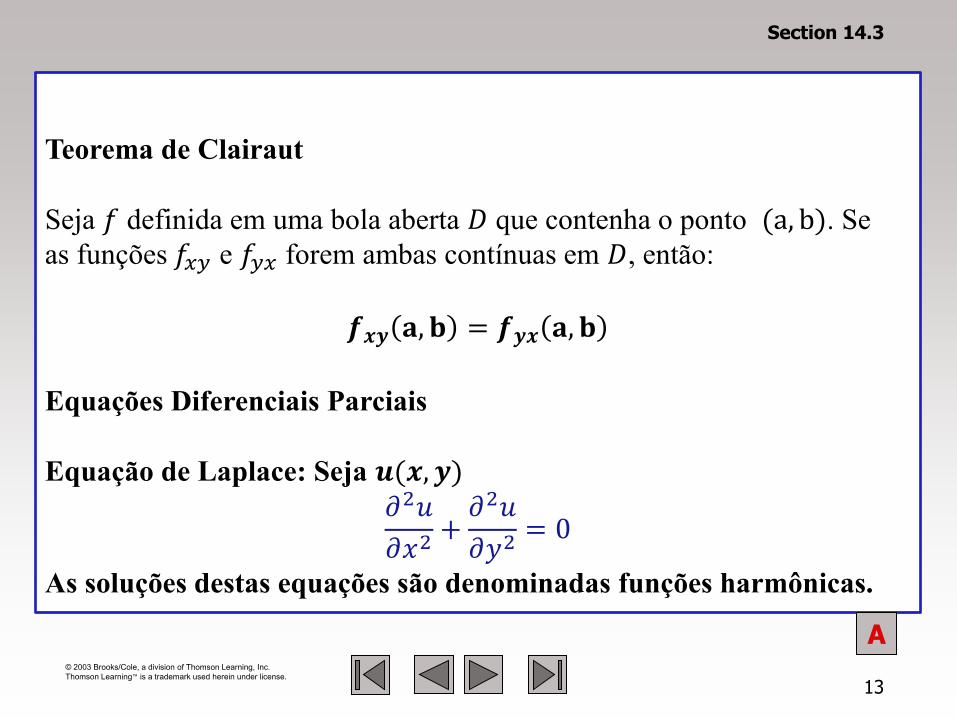
Teorema de Clairaut
Seja 𝑓 definida em uma bola aberta 𝐷 que contenha o ponto (a, b). Se
as funções 𝑓𝑥𝑦 e 𝑓𝑦𝑥 forem ambas contínuas em 𝐷, então:
𝒇𝒙𝒚 𝐚, 𝐛 = 𝒇𝒚𝒙 𝐚, 𝐛
Equações Diferenciais Parciais
Equação de Laplace: Seja 𝒖(𝒙, 𝒚)
𝜕2𝑢
𝜕𝑥2 +𝜕2𝑢
𝜕𝑦2 = 0
As soluções destas equações são denominadas funções harmônicas.
Section 14.3
A


