20180305093318 c M. K. Warby MA2715 Advanced Calculus and Numerical Methods 0–1 MA2715 Advanced Calculus and Numerical Methods Lecture Notes by M.K. Warby in 2017/8 Dept. of Mathematics, Brunel Univ., UK Email: [email protected]URL: http://people.brunel.ac.uk/ ~ icstmkw/ma2715/ MA2715 and MA2895 – the week breakdown The lectures MA2715 run for weeks 17-26,30-31 with seminars starting in week 18. The related assessment block MA2895 will run with teaching events for weeks 17–26 involving computer labs in which Matlab will be used. Assessment dates and assessment information Some of the assessment is under the code MA2895_CB which is a 10 credit module which has the title “Numerical Analysis Project” and for this the breakdown is as follows: • Class test worth 30%: Planned for week 21. • Assignment worth 70%: Deadline is likely to be the start of week 27. The assignment tasks are likely to be given out in two or three weeks with some of the topics related to the material of MA2715. We will confirm later as to the precise arrangement of the test planned for week 21 and also the deadline for the assignment. There will also be questions on the material taught on all parts of MA2715_SB in the 20 credits assessment block MA2815_CN which has the title “Advanced Mathematics II and Numerical Methods”. This exam will be in the May 2018 exam period.
The lectures MA2715 run for weeks 17-26,30-31 with seminars starting in week 18.
The related assessment block MA2895 will run with teaching events for weeks 17–26involving computer labs in which Matlab will be used.
Assessment dates and assessment information
Some of the assessment is under the code MA2895_CB which is a 10 credit module whichhas the title “Numerical Analysis Project” and for this the breakdown is as follows:
• Class test worth 30%: Planned for week 21.
• Assignment worth 70%: Deadline is likely to be the start of week 27. The assignmenttasks are likely to be given out in two or three weeks with some of the topics relatedto the material of MA2715.
We will confirm later as to the precise arrangement of the test planned for week 21and also the deadline for the assignment.
There will also be questions on the material taught on all parts of MA2715_SB in the20 credits assessment block MA2815_CN which has the title “Advanced Mathematics IIand Numerical Methods”. This exam will be in the May 2018 exam period.
There is no essential text to obtain for this module although there are many texts whichcover at least most of the material and among the sources for the notes that I will generateare the following books.
2. Richard L. Burden and J. Douglas Faires. Numerical analysis. Brooks/Cole, 7thedition, 2001.QA297.B87. The Brunel library has later editions with the 9th edition being pub-lished in 2011.
3. David F. Griffiths and Desmond J. Higham. Numerical Methods for Ordinary Dif-ferential Equations. Initial Value Problems. Springer, 2010. ISBN: 9781280391163.Electronic access available via Brunel library catalogue web pages.
(This is only for a chapter about the initial value problem which will only to beconsidered briefly.)
(Chapter 7 contains material about Fourier series which is likely to be the lastchapter covered in MA2715.)
Books about Matlab related to MA2895
The following is repeated in the handouts for the Matlab sessions and for completeness Iinclude it here as well. There is no core Matlab book that you have to buy for the modulealthough I do myself own several books and among those that I consult sometimes arethe following.
2. Brian D. Hahn and D. T. D. T. Valentine. Essential MATLAB for engineers andscientists. Academic Press, 5th edition, 2013.QA297.H345. Only the 4th edition is currently in the Brunel library.
3. D. J. Higham and Nicholas J. Higham. MATLAB guide. Society for Industrial andApplied Mathematics, 2nd edition, 2005.QA297.H525
(A 3rd edition was published in Feb 2017.)
Please note that Matlab itself has an extensive help system.
In this module the following notation will be used.
R denotes the set of real numbers.
Rn denotes the set of vectors of length n with real entries.
Rm,n denotes the set of matrices with m rows and n columns with real entries.
For column vectors the notation x = (xi) ∈ Rn is shorthand for a real column vector xwith n rows with the row i entry being xi, i.e.
x =
x1...xn
.
If x is a column vector then xT = (x1, . . . , xn) is a row vector. Here the superscript T
denotes transpose. Column vectors and row vectors are special cases of a matrix andin the notation used we have reduced how much we write by just using 1 subscript forthe entries. When both m > 1 and n > 1 we have a matrix and we use the notationA = (aij) ∈ Rm,n as shorthand for a real matrix with m rows and n columns with the i, jentry being aij, i.e.
A =
a11 · · · a1n... · · · ...am1 · · · amn
.
When we refer to the size of a matrix the terms m-by-n or m×n will sometimes be used.In this module we mostly just consider the case when m = n, i.e. we mostly just considersquare matrices.
Other notation which will frequently be used are the following.
– Vectors and matrices: notation, revision and norms – 1–1 –
The zero vector is denoted by 0. The size of 0 will be depend on the context.
The n× n identity matrix is denoted by
I = (δij) =
1 0 0 · · · 00 1 0 · · · 00 0 1 · · · 0...
......
. . ....
0 0 0 · · · 1
,
where
δij =
{1, if i = j,
0, otherwise.
The identity matrix is a square diagonal matrix with each diagonal entry being equal to 1.When just I is written the size should be clear from the context but if the size is notimmediately clear then we will write In when the size is n× n.
The standard base vectors for Rn are denoted by e1, . . . , en which correspond respec-tively to the columns of I. Thus when n = 3 we have
I = I3 =
1 0 00 1 00 0 1
, e1 =
100
, e2 =
010
, e3 =
001
.
1.2 The vector space Rn
Rn is an example of a vector space and the vectors e1, . . . , en give the standard basis forthis space and further these base vectors are orthonormal. (Vector spaces were discussedat the start of level 2 as part of the module MA2721.) We consider next the definitions ofthese terms using the column vector notation used in this module.
The inner product of vectors x and y is defined by
xTy = (x1, x2, . . . , xn)
y1y2...yn
= x1y1 + x2y2 + · · ·+ xnyn.
In books and other sources you may see this operation written as (x, y) or < x, y > or asx ·y but in these notes the matrix product notation of a row vector times a column vectorwill be used.
Vectors x and y are orthogonal if
xTy = 0.
A vector x has unit length if
xTx = x21 + · · ·+ x2n = 1.
– Vectors and matrices: notation, revision and norms – 1–2 –
(As we will see in section 1.5, for vectors x of any length the quantity xTx is also referredto as the square of the 2-norm of x.)
Vectors v1, . . . , vn are orthonormal if the vectors each have unit length and they areorthogonal to each other, i.e.
vTi vi = 1, i = 1, . . . , n and vTi vj = 0, when i 6= j.
Vectors v1, . . . , vn are linearly independent if
α1v1 + · · ·+ αnvn = 0
is only true if α1 = · · · = αn = 0. It follows almost immediately that if vectors are or-thonormal then they are linearly independent. The converse of linearly independent is lin-early dependent. Vectors v1, . . . , vn are linearly dependent if there exists α = (αi) 6= 0such that
α1v1 + · · ·+ αnvn = 0.
1.3 The vector Ax and the solution of Ax = b
In the context of things done in MA2715 note that when we have a n× n matrix A and an× 1 column vector x the product gives another column vector, i.e.
b = Ax ∈ Rn.
This can be represented in a number of ways. With b = (bi) the matrix multiplicationmeans that
bi = (ith row of A)x =n∑j=1
aijxj, i = 1, . . . , n.
Instead of considering things entry-by-entry we can consider representing A column -by-column, i.e.
A = (a1, . . . , an) where aj =
a1j...anj
= jth column of A.
It is valid here to write
Ax = (a1, . . . , an)
x1...xn
= a1x1 + · · ·+ anxn
= x1a1 + · · ·+ xnan.
Provided the matrix sizes are compatible matrix multiplication works in “block form”to explain how the second line follows from the first line. The final line follows becauseaj xj = xjaj as a consequence of what we mean by a scalar times a vector. The point of
– Vectors and matrices: notation, revision and norms – 1–3 –
writing the expression in this form is that Ax is a linear combination of the n columns ofA. When the columns of A are linearly dependent there is a vector x 6= 0 such that
Ax = 0
and this vector is an eigenvector of A with 0 as the eigenvalue. When the columns of Aare linearly dependent the matrix is singular, the determinant detA = 0, the matrix doesnot have an inverse matrix (i.e. it is not invertible) and we cannot uniquely solve a linearsystem
Ax = b.
In chapter 2 we consider how computer packages solve Ax = b and we hence need todetermine when there is a unique solution and when there is not, i.e. as part of thecomputation we need to be able to decide if the matrix A is a singular matrix or not. Inyour previous study you will have done many examples with small matrices (e.g. n = 2or n = 3) where you attempt to obtain a solution or you detect that there is no uniquesolution and you possibly also determine a general solution if it exists. For larger matriceswith computations done on a computer with floating point arithmetic used (which usuallyhas rounding errors) we cannot generally be so precise in deciding that a matrix is singularbut instead be can just determine that a matrix is “close to being singular”. This isdescribed briefly in section 1.5 when vector and matrix norms and the matrix conditionnumber is introduced.
1.4 Eigenvalues and eigenvectors
Eigenvalues and eigenvectors will appear a few times in this module and we give herebriefly a revision of the definition of these terms together with some of the basic properties.
Let A denote a real n × n matrix. A vector v 6= 0 is an eigenvector of A witheigenvalue λ if
Av = λv.
This can be equivalently written as
Av − λv = 0 or (A− λI)v = 0.
As v 6= 0 this means that we have a non-trivial solution of (A−λI)v = 0 and this impliesthat A− λI is singular and its determinant is 0. If we let
pA(t) = det(A− tI)
then this defines the characteristic polynomial of A, and the eigenvalues are the rootsof this polynomial. As a minor point, the characteristic polynomial is often defined asdet(tI−A), e.g. this is the case in Matlab, which only differs from the previous definitionby a factor of −1 when n is odd and both versions have the same roots which are thesolutions of
det(A− λI) = 0
which is known as the characteristic equation. There is a result known as the funda-mental theorem of algebra which states that such a polynomial has n roots λ1, . . . , λnin the complex plane such that
PA(t) = (λ1 − t)(λ2 − t) · · · (λn − t)
– Vectors and matrices: notation, revision and norms – 1–4 –
which is a polynomial of degree n. The set of eigenvalues {λ1, . . . , λn} is known as thespectrum of A. The spectral radius of a matrix is defined by
ρ(A) = max {|λ1|, . . . , |λn|} .
As a final comment here, as A is a real matrix the polynomial pA(t) has real coefficientsand as a consequence any non-real roots of pA(t) must occur in complex conjugate pairs.
1.4.1 Examples
1. Let
A = I2 =
(1 00 1
).
Then
pA(t) = det(I2 − tI2) =
∣∣∣∣1− t 00 1− t
∣∣∣∣ = (1− t)2.
The eigenvalues are λ1 = λ2 = 1, i.e. we have a repeated eigenvalue. Every non-zerovector in R2 is an eigenvector.
2. Let
A =
(2 11 2
).
Then
pA(t) =
∣∣∣∣2− t 11 2− t
∣∣∣∣ = (2− t)2 − 1 = (1− t)(3− t).
The eigenvalues are λ1 = 1 and λ2 = 3. To get an eigenvector corresponding toλ1 = 1 we need to obtain a non-zero solution to
(A− λ1I)x =
(1 11 1
)(x1x2
)=
(00
).
A solution is xT = (1,−1).
Similarly to get an eigenvector corresponding to λ2 = 3 we need to obtain a non-zerosolution to
(A− λ2I)x =
(−1 11 −1
)(x1x2
)=
(00
).
A solution is xT = (1, 1).
Observe that the eigenvector corresponding λ1 is orthogonal to the eigenvector cor-responding to λ2 which is a consequence of the matrix being real and symmetric.The spectral radius of this matrix is max {1, 3} = 3.
3. Let
A =
(0 −11 0
).
Then
pA(t) =
∣∣∣∣−t −11 −t
∣∣∣∣ = t2 + 1 = (i− t)(−i− t).
– Vectors and matrices: notation, revision and norms – 1–5 –
The eigenvalues are the complex conjugate pair λ1 = i and λ2 = −i. The eigen-vectors are also complex. The spectral radius of this matrix is 1. The matrix isa rotation matrix corresponding to anti-clockwise rotation by angle π/2 about theorigin.
4. Let
A =
(0 10 0
).
Then
pA(t) =
∣∣∣∣−t 10 −t
∣∣∣∣ = t2.
The eigenvalues are λ1 = λ2 = 0. To obtain an eigenvector we need to obtain anon-zero solution of
(A− 0I)x =
(0 10 0
)(x1x2
)=
(00
).
The only information that these equations give is that x2 = 0 and thus the onlydirection which is an eigenvector is xT = (1, 0). This is an example of a deficientmatrix in that it has an eigenvalue of algebraic multiplicity equal to 2 (this is fromconsidering the characteristic polynomial) but the dimension of the eigen-subspacecorresponding to this eigenvalue is only 1. The dimension of the eigen-subspacecorresponding to an eigenvalue is known as the geometric multiplicity.
Note that in this example the spectral radius is 0 but the matrix is not the zeromatrix although A2 is the zero matrix. This example shows that for general matricesthe spectral radius cannot be used to define a norm for square matrices with normsconsidered soon in this chapter.
1.4.2 A summary of key points about eigenvalues and eigenvec-tors
Let vi 6= 0 denote an eigenvector associated with the eigenvalue λi, i.e.
Avi = λivi, i = 1, 2, . . . , n.
The following are some important results about eigenvalues which are needed in thismodule.
1. An n× n matrix A is non-singular if and only if λi 6= 0 for i = 1, 2, . . . , n.
2. If v1, . . . , vn are linearly independent then they give a basis for Rn. In matrix formwe have
A(v1, . . . , vn) = (Av1, . . . , Avn)
= (λ1v1, . . . , λnvn)
= (v1, . . . , vn)
λ1 . . .
λn
.
– Vectors and matrices: notation, revision and norms – 1–6 –
If we let V = (v1, . . . , vn) be the matrix with the columns as the eigenvectors andwe let D = diag(λ1, . . . , λn) then in matrix form we have
AV = V D.
As we are assuming that the columns of V are linearly independent it follows thatV has an inverse and we can write
V −1AV = D and A = V DV −1.
The first result is often referred to as diagonalising the matrix and the second versiongives a representation of the matrix in terms of the eigenvalues and eigenvectors.Using this representation we can immediately get powers of A as
A2 = (V DV −1)(V DV −1) = V D2V −1
and more generallyAk = V DkV −1, k = 1, 2, . . . .
When all the eigenvalues are non-zero we also have
A−1 = V D−1V −1.
3. If λ1, . . . , λn are distinct then it can be shown that the eigenvectors v1, . . . , vn arelinearly independent and the conditions in the previous item hold.
4. If A is a real symmetric matrix then we can diagonalise A using an orthogonalmatrix, i.e. there exists an orthogonal matrix Q such that
QTAQ = D, A = QDQT . (1.4.1)
This is a special case of the situation above with V = Q as the inverse of anorthogonal matrix is its transpose, i.e. Q−1 = QT .
1.5 Vector and matrix norms
For a given object (vectors and matrices in our case) a norm is a way of giving a ‘size’ tothe object. For example the modulus of a real or complex number defines a norm and theEuclidean length of a vector in three dimensional geometry defines a norm. With a wayof giving a size to objects like vectors and matrices we can then consider when a vectorx is close to another vector y by considering the size of x− y and we can consider whena matrix A is close to another matrix B by considering the size of A−B. In the contextof solving Ax = b situations like these arise when we have an approximate solution x andwe need to estimate or compute the size of the error x − x and the size of the residualterm b− Ax.
In the n dimensional space Rn there are many different norms which can be definedand we will consider the most popular ones shortly. In the applications that are consideredin this module it does not usually matter too much which norm is used as in a certainsense all norms in Rn are equivalent which roughly means that if ‖x‖ is very small orvery big in one norm then it is also very small or very big respectively in another normprovided n is not too large.
– Vectors and matrices: notation, revision and norms – 1–7 –
We begin abstractly by giving the vector norm axioms.
A function f : Rn → R is a vector norm if the following conditions are satisfied:
(i) f(x) ≥ 0 for all x ∈ Rn with f(x) = 0 if and only if x = 0.
(ii) f(αx) = |α|f(x) for all α ∈ R, x ∈ Rn. (This is linearity.)
(iii) f(x+ y) ≤ f(x) + f(y) for all x, y ∈ Rn. (This is the Triangle inequality.)
If f is a norm then we use the notation
f(x) = ‖x‖ .
(When more than one norm is being used or when the particular norm being used isnot clear from the context we will use subscripts to distinguish between different norms.)
In this ‖.‖ notation we repeat the norm axioms as follows:
(i) ‖x‖ ≥ 0 for all x ∈ Rn with ‖x‖ = 0 if and only if x = 0.
(ii) ‖αx‖ = |α| ‖x‖ for all α ∈ R and x ∈ Rn.
(iii) ‖x+ y‖ ≤ ‖x‖+ ‖y‖ for all x and y in Rn.
1.5.2 Commonly used vector norms
The most commonly used vector norms are the 2-norm, the ∞−norm and the 1− normand for x ∈ Rn these are defined as follows.
‖x‖2 =(x21 + x22 + · · ·+ x2n
)1/2=
(n∑1
x2i
)1/2
=(xTx
)1/2is the 2-norm or Euclidean norm. (When we just refer to the length of a vector it isusually understood that this means the two norm.) In usage the next most popular normis
‖x‖∞ = max1≤i≤n
|xi|
which is the ∞-norm. The 1-norm is
‖x‖1 = |x1|+ |x2|+ · · ·+ |xn| =n∑1
|xi|.
There is a function called norm() in Matlab which computes these norms. For example,if you put
– Vectors and matrices: notation, revision and norms – 1–8 –
norm(x) and norm(x, 2) both give the 2-norm whilst in the other cases a second argumentof inf or 1 has to be given.
As a final comment on the definition of the 2-norm, if we need to consider vectors withnon-real entries then we need to change slightly what is given above to be such that
‖x‖22 = |x1|2 + · · ·+ |xn|2 =n∑i=1
|xi|2 = xTx.
Here the notation x = (xi), means that each entry is the complex conjugate of thecorresponding entry of x = (xi). In a later chapter there will be examples involving realmatrices which have complex eigenvalues and eigenvectors but there will not be too manyother examples in this module when we have vectors with non-real entries.
1.5.3 Matrix norms induced by vector norms
Let A denote a n× n matrix. Given any vector norm for vectors in Rn we can define thematrix norm of A induced by the vector norm as
‖A‖ = max {‖Ax‖ : ‖x‖ = 1} . (1.5.1)
It is straightforward to show that a similar set of axioms to the vector case also hold here.More precisely we have the following.
(i) ‖A‖ ≥ 0 for all A ∈ Rn,n with ‖A‖ = 0 if and only if A = 0.(A = 0 means A=zero matrix.) This is known as the non-negative condition.
(ii) ‖αA‖ = |α| ‖A‖ for all scalars α ∈ R and all A ∈ Rn,n. This is known as thelinearity condition.
(iii) ‖A+B‖ ≤ ‖A‖+ ‖B‖ for all A,B ∈ Rn,n. This is known as the triangle inequality.
– Vectors and matrices: notation, revision and norms – 1–9 –
We can add to these properties if we consider matrix-vector multiplication and matrix-matrix multiplication.
In the first case, an immediate consequence of the definition of the matrix norm isthat if we consider a vector x 6= 0 then
y =x
‖x‖
is a vector of norm 1 in the norm being used and
x = ‖x‖ y
so that‖Ax‖ = ‖x‖ ‖Ay‖ ≤ ‖x‖ ‖A‖.
Thus for all vectors x ∈ Rn we have
‖Ax‖ ≤ ‖A‖ ‖x‖ (1.5.2)
and for at least one direction there is a vector x with ‖Ax‖ = ‖A‖ ‖x‖.
In the case of matrix-matrix multiplication we have that if A and B are both n × nmatrices then the products AB and BA are also n×n matrices. If x is such that ‖x‖ = 1then ABx = A(Bx) and thus
‖ABx‖ ≤ ‖A‖ ‖Bx‖, using (1.5.2) in the case of the matrix A,
≤ ‖A‖ ‖B‖ ‖x‖, using (1.5.2) in the case of the matrix B,
= ‖A‖ ‖B‖, as the vector x has norm 1.
Thus‖AB‖ = max {‖ABx‖ : ‖x‖ = 1} ≤ ‖A‖ ‖B‖.
Similarly‖BA‖ ≤ ‖A‖ ‖B‖.
These indicate that we can bound the norm of the product of two matrices in terms ofthe norms of the matrices involved and in particular note that it follows that
‖Ak‖ ≤ ‖A‖k, k = 1, 2, . . . .
1.5.4 The matrix norms ‖A‖1, ‖A‖2 and ‖A‖∞
Each of the common vector norms generates an induced matrix norm and it turns outthat it is not too difficult to get explicit expressions for these although we omit the detailsof the derivations in these notes although some these are considered in the exercise sheetquestions. We use the notation ‖A‖1, ‖A‖2 and ‖A‖∞ for the matrix norms induced bythe vector 1-norm, 2-norm and ∞-norm respectively. The results are as follows.
– Vectors and matrices: notation, revision and norms – 1–10 –
These results show that it is straightforward to compute ‖A‖∞ and ‖A‖1 but that thematrix 2-norm involves computing the dominant eigenvalue of ATA which can usuallyonly be done numerically and it involves much more work than the other two cases.
As an example, consider the following 3 × 3 matrix which is on the wiki-page aboutmatrix norms.
A =
3 5 72 6 40 2 8
.
The row sums of the absolute values are 15, 12 and 10 and thus ‖A‖∞ = 15. The columnsums of the absolute values are 5, 13 and 19 and thus ‖A‖1 = 19. We can use Matlab towork out the 2-norm and this can be done by the following commands
A=[3, 5, 7; 2, 6, 4; 0, 2, 8]
ninf=norm(A, inf)
n1=norm(A, 1)
n2=norm(A)
which generate the following output
A =
3 5 7
2 6 4
0 2 8
ninf = 15
n1 = 19
n2 = 13.686
1.6 The spectral radius and matrix norms
There are some connections between the spectral radius ρ(A) of a matrix A and any ofthe induced matrix norms ‖A‖.
– Vectors and matrices: notation, revision and norms – 1–11 –
Firstly, if v 6= 0 is an eigenvector of A with eigenvalue λ, i.e. Av = λv then any scalingof v is also an eigenvector and thus there is a eigenvector corresponding to λ such that‖v‖ = 1. In this case
|λ| = |λv| = ‖Av‖ ≤ ‖A‖.
This shows that an induced matrix norm is a bound on the magnitude of all the eigenvaluesare thus in particular
ρ(A) ≤ ‖A‖.
As we can easily compute ‖A‖1 and ‖A‖∞ we get that
ρ(A) ≤ min {‖A‖1, ‖A‖∞} .
Secondly, if the matrix is real and symmetric, i.e. A ∈ Rn×n and AT = A, then‖A‖1 = ‖A‖∞ and
‖A‖22 = ρ(ATA) = ρ(A2).
When we have a real symmetric matrix all the eigenvalues are real and for any matrix
Av = λv implies that A2v = A(λv) = λ2v.
The eigenvalues of A2 are the square of the eigenvalues of A and thus in the real symmetriccase
‖A‖2 = ρ(A) = max {|λi| : λi is an eigenvalue of A} .
As we still have bounds on ρ(A) by using ‖A‖1 = ‖A‖∞ it follows that in the realsymmetric case
‖A‖2 = ρ(A) ≤ ‖A‖1 = ‖A‖∞.
1.7 The matrix condition number
When A is a n × n matrix which is non-singular it has an inverse A−1 and the matrixcondition number is defined as
κ(A) = ‖A‖ ‖A−1‖.
When A is singular we say that κ(A) =∞. From the result that ‖AB‖ ≤ ‖A‖ ‖B‖, thatI = A−1A and that ‖I‖ = 1 it follows that for all square matrices
1 ≤ κ(A) ≤ ∞.
This quantity can be expressed in terms of eigenvalues when we have a real symmetricmatrix as when all the eigenvalues of A are non-zero the relation
Av = λv rearranges to A−1v =
(1
λ
)v.
Thus if the eigenvalues of a non-singular matrix A are λ1, . . . , λn then the eigenvalues ofA−1 are λ−11 , . . . , λ−1n . If for convenience we suppose that the labelling is such that
0 < |λn| ≤ · · · ≤ |λ1|
– Vectors and matrices: notation, revision and norms – 1–12 –
The significance of the condition number to this module is that a large conditionnumber indicates that the matrix is close to a singular matrix and we cannot expect toaccurately solve a linear system Ax = b by any means. With some further analysis it canbe shown that 1/κ(A) gives the relative distance of the matrix A to a singular matrix,i.e. for all singular matrices C of the same size as A we have
‖A− C‖‖A‖
≥ 1
κ(A).
and there exists a singular matrix B such that
‖A−B‖‖A‖
=1
κ(A).
In the case of the 2-norm the nearest singular matrix B to the non-singular matrix A canbe quite easily described by using what is known as the singular valued decomposition ofA which is a topic beyond this module. In the particular case that A is real and symmetricthe situation is slightly easier by noting that we have the representation of A in terms ofeigenvalues and eigenvectors given in (1.4.1)
A = QDQT
= λ1v1 vT1 + · · ·+ λn−1vn−1 v
Tn−1 + λnvn v
Tn .
If we replace the smallest eigenvalue in magnitude (which is λn) by 0 then we get a singularmatrix. If we denote this singular matrix by B then it has the representation
B = λ1v1 vT1 + · · ·+ λn−1vn−1 v
Tn−1
and it can be shown that this is the nearest singular matrix to the matrix A with
‖A−B‖2 = |λn|, ‖A‖2 = |λ1| and‖A−B‖2‖A‖2
=|λn||λ1|
.
– Vectors and matrices: notation, revision and norms – 1–13 –
In this chapter we consider Gauss elimination type methods for a solving a system oflinear equations
Ax = b,
where A is an n×n matrix and b is a n× 1 column vector. Methods of this type are usedin Matlab when you give the command
x=A\b;
when A and b have the appropriate shape in the Matlab workspace. In fact when youput A\b in Matlab the software attempts to classify the type of matrix involved andthen selects the “best” technique to use to reliably solve the problem in an efficient way.Different methods are used if for example the matrix is symmetric or if it is tri-diagonalas compared to what is done if A is a full matrix with no special properties. (Thesymmetric case also needs a property known as positive definite.) In this chapter wejust consider this general case and consider in general the Gauss elimination procedureinvolving systematically reducing a general system to an equivalent system involving atriangular matrix. A key result of the chapter is in showing that the Gauss eliminationprocess is equivalent to factorizing the matrix A in terms of triangular matrices, i.e. inits basic form (when it works) we show that we get the factorization
A = LU,
where L is a unit lower triangular matrix and U is an upper triangular matrix.In the case that n = 4 this means that we have a factorization of the form
An upper triangular matrix is a matrix for which all the entries below the diagonal are 0,a lower triangular matrix is a matrix for which all the entries above the diagonal are 0
and a unit lower triangular matrix is a lower triangular matrix with the diagonal entriesall being equal to 1. For Gauss elimination to work in its basic form needs A to havespecial properties. For a more stable way of factorizing a matrix packages instead createa factorization of the form
PA = LU,
where P is permutation matrix. In this form the matrix PA is obtained from A byrearranging the rows. In Matlab you can get the matrices generated by using the command
[L, U, P]=lu(A);
Gauss elimination and implementations involving LU factorization are examples ofdirect methods for solving Ax = b where the term direct method means that theexact solution is obtained in a finite number of steps provided exact arithmetic is used.However it should be realised that to do computations quickly on a computer floatingpoint arithmetic is used and this has rounding error with calculation typically done withclose to 16 decimal digit accuracy. Thus in practice we only get an approximate solutionalthough hopefully the method can generate an approximate solution which is close tomachine accuracy.
2.2 Forward and backward substitution algorithms
We start by considering systems with triangular matrices and we start with two exampleswhich can be done by hand calculations.
The last equation only involves x4 and hence we get this immediately. Then using x4 wecan use the previous equation to get x3 and continue in a similar way to get x2 and thenx1. For the details
4x4 = 4, giving x4 = 1,
3x3 = −2− x4, giving x3 = −1,
2x2 = 3− x3, giving x2 = 2,
x1 = −x3, giving x1 = −2.
Next consider the lower triangular system1 0 0 01 1 0 01 1 1 01 1 1 1
The first equation only involves x1 and hence we get this immediately. Then using x1 wecan use the second equation to get x2 and continue in a similar way to get x3 and thenx4. For the details
x1 = 2,
x2 = 3− x1, giving x2 = 1,
x3 = 2− x1 − x2, giving x3 = −1,
x4 = −x1 − x2 − x3, giving x4 = −2.
The procedure used in the case of an upper triangular matrix is known as backwardsubstitution and the procedure used in the case of the lower triangular system is knownas forward substitution. We now consider how to do this generally for n×n triangularmatrices. For a general upper triangular system Ux = b, i.e.
backward substitution can be described as follows.
xn = bn/unn
xi =
(bi −
n∑k=i+1
uikxk
)/uii, i = n− 1, . . . , 1 .
For a general lower triangular system Lx = b, i.e.
l11x1 = b1l21x1 + l22x2 = b2
......
ln1x1 + · · · + ln,n−1xn−1 + ln,nxn = bn
forward substitution can be described as follows.
x1 = b1/l11
xi =
(bi −
i−1∑k=1
likxk
)/lii, i = 2, . . . , n .
In both cases the procedure requires that the diagonal entries are non-zero as we divideby these entries.
In algorithms implemented on a computer using floating point arithmetic an operationinvolving 1 multiplication and 1 addition/subtraction is sometimes referred to as a flopalthough it seems now more common to refer to this as 2 flop operations as 2 operationsare involved and this is what will be done here. The computational cost of an algorithmis often expressed in terms of how many such operations are needed to solve a problem.The speed of a computer is also often expressed in terms of how many of such operationscan be done in 1 second (the terms flops is used in this case). In the case of the number
of operations involved in the backward or forward substitution this can be determinedwithout too much effort and in the case of forward substitution the computation of
bi −i−1∑k=1
likxk
involves 2(i− 1) flop operations and this must be done for i = 2, . . . , n. In total this gives
2(1 + 2 + 3 + · · ·+ (n− 1)) = n(n− 1).
When n is large there is a much smaller number of divisions and we say that in total thereis an the order of n2 operations which is often written as O(n2). The operation countwith backward substitution is the same. Thus in each case the triangular matrices involveO(n2/2) entries and the number of operations needed to solve the systems is O(n2).
2.3 Solving a system LUx = b
Before we consider how to obtain a factorization A = LU we consider briefly how thishelps us to solve a system of equations
Ax = LUx = b,
i.e. we start by assuming that we have a lower triangular matrices L and an uppertriangular U such that A = LU . All we do is to let y = Ux and first solve a systemLy = b and once we have y we solve a second system Ux = y to get x. To express this asan algorithm we have the following.
Solve Ly = b by forward substitution.
Solve Ux = y by backward substitution.
The number of operations involved is O(2n2). This is much less operations than thenumber of operations needed to get the triangular matrices L and U which we showneeds O(2n3/3) operations as we describe in the next section.
2.4 Reduction to triangular form by Gauss elimina-
tion
In Gauss elimination you eliminate unknowns by subtracting appropriate multiples of oneequation from the other equations and in terms of the coefficients this involves subtractingmultiples of one row from other rows. In the case that n = 4 the sequence of matricesgenerated by basic Gauss elimination has the following form.
In each case x just indicates an entry which is likely to be non-zero and in the above weare just considering the changes in the matrix without considering the changes that arealso done to the right hand side vector. The first matrix refers to the starting matrix Aand the final matrix is an upper triangular matrix which we refer to as U . There are 3steps here with each step associated with creating zero entries below the diagonal in agiven column. In the case of a general n× n matrix there are n− 1 such steps.
There is a choice at each stage as to which row you use to subtract multiples of fromthe other rows and there is even the possibility of re-ordering the unknowns which involvesre-ordering the columns. In the basic version of Gauss elimination none of the above isdone and we always subtract multiples of the current top row from the rows below. Thusin the basic form you are not also making decisions about which row to use to make thehand computations as easy as possible and you are not changing one row by multiplyingit by a scalar as you may have done when dealing with small matrices in level one. BasicGauss elimination is hence one specific order of the operations that you were taught atlevel one in the context of solving a linear system and we consider next how to describethis in a matrix way and we show that it is equivalent to a factorization.
To describe the operations in a matrix way let A(0) = A and let A(k), k = 1, . . . , n− 1denote the intermediate matrices with U = A(n−1) denoting the final upper triangularmatrix assuming the procedure runs to completion. In the case n = 4 the matrices are
As a consequence of the order in which the reduction is done the first row never changes,the second row never changes once A(1) has been computed, the third row never changesonce A(2) has been computed and the final entry to be computed is the 4, 4 entry of U .We show next how to describe each reduction step as a matrix multiplication with
A(1) = M1A(0), A(2) = M2A
(1), U = A(3) = M3A(2)
so thatU = M3M2M1A
andA = (M3M2M1)
−1U = (M−11 M−1
2 M−13 )U = LU
whereL = M−1
1 M−12 M−1
3 .
The matrices Mk are known as Gauss transformation matrices, which are described in amoment, and we will show that the matrix L is a unit lower triangular matrix.
Firstly, to obtain A(1) we subtract multiples of the first row from rows 2, 3 and 4. Nowthe first row at this stage is (
The next task is describe the inverse matrices M−11 , M−1
2 and M−13 and the product
of these which is L = M−11 M−1
2 M−13 . This is very straightforward as
M−1k = I +mke
Tk , k = 1, 2, 3.
This follows by noting that at the kth stage the kth row does not change and thus we canreverse the reduction process by adding the same multiples of the kth row to the otherrows. Alternatively we can verify the expression for the inverse by just considering theproduct
(I −mkeTk )(I +mke
Tk ) = I −mk(e
Tkmk)e
Tk = I
where the last equality is because
eTkmk = kth entry of mk = 0
as mk has entries of 0 in positions 1, . . . , k. For the product of these matrices first notethat
which is a unit lower triangular matrix and the entries below the diagonal are exactly themultipliers used in the basic Gauss elimination process.
The general n× n case
The above description easily generalises to the case of a general n × n matrix whichrequires elimination below the diagonal in columns 1, 2, . . . , n−1 and this involves matricesA(0) = A, A(1), . . . , A(n−1) = U . In the general case we have for k = 1, . . . , n− 1,
A(k) = MkA(k−1), Mk = I −mke
Tk , mk =
0...0
mk+1,k...
mnk
.
In the above the multipliers are
mik =a(k−1)ik
a(k−1)kk
, i = k + 1, . . . , n, (2.4.1)
the inverse matrices areM−1
k = I +mkeTk
and for the product we have
M−11 · · ·M−1
r = I +m1eT1 + · · ·+mre
Tr , r = 2, . . . , n− 1.
This can be proved by induction and there is an exercise question about this. For thealgorithm to run to completion we need the matrix to be such that we never divide by 0,i.e. we need that a
(k−1)kk 6= 0 for k = 1, . . . , n − 1 and also for U to be invertible we need
that a(n−1)nn 6= 0. The terms ukk = a
(k−1)kk are the pivot elements and they are the diagonal
entries of U (assuming that the algorithm runs to completion to create U).
To count the number of operations involved note that to get A(1) from A involvescomputing (n − 1)2 entries corresponding to positions 2 ≤ i, j ≤ n and there are 2floating point operation associated with each entry. Similarly to get A(2) from A(1) requireschanging (n − 2)2 entries with 2 operations in each case and continuing in this way thetotal reduction process requires the following number of operations
It is not necessary to be too precise here other than to note that we have the n3 term andwe can get the constant 2/3 by considering the integral 2
∫ n0x2 dx as the area under the
curve y = 2x2 is similar in some sense to the sum. Hence as we double the size of a matrixwe get 4 times as many entries and we require about 8 times as much work to solve asystem Ax = b when A is a full matrix with no special properties. This operation countshould be compared with the forward and backward substitution algorithms which justhas a term of involving n2. The point here to note is that for large matrices the reductionto triangular form is where most of the computation is done.
Example
Let
A =
2 3 1−2 −2 −2−2 −4 4
.
The Gauss elimination procedure to construct the LU factorization involves the followingsteps.
Elimination in column 1:
m1 =
0−1−1
, A(1) =
2 3 10 1 −10 −1 5
.
Elimination in column 2:
m2 =
00−1
, U = A(2) =
2 3 10 1 −10 0 4
.
The unit lower triangular matrix is
L = I +m1eT1 +m2e
T2 =
1 0 0−1 1 0−1 −1 1
.
Thus we have shown that 2 3 1−2 −2 −2−2 −4 4
=
1 0 0−1 1 0−1 −1 1
2 3 10 1 −10 0 4
.
To check the calculations using Matlab all that is needed is to put the following.
It is worth noting here that the Matlab command lu will not necessarily give the LUfactorization when used in this way as it always uses pivoting which is described shortly. Inthis particular example the pivoting decisions was that nothing needed to be re-arranged.
The factorization of sub-matrices
For a n× n matrix A = (aij) the k × k principal sub-matrix isa11 · · · a1k... · · · ...ak1 · · · akk
.
In the previous example we can immediately note that for the sub-matrices of sizek = 1 and k = 2 we have
2 = (1)(2)
and (2 3−2 −2
)=
(1 0−1 1
)(2 30 1
).
This shows that in this example the factorization of the full matrix also gives the factor-ization of all the principal sub-matrices. To prove that this is true in general we just needto consider what matrix multiplication means when we have A = LU with A = (aij),L = (lij) and U = (uij).
aij = (LU)ij = (ith row of L)(jth column of U)
=n∑r=1
lirurj
=
min{i,j}∑r=1
lirurj
where the last equality is because L and U are triangular and thus lir = 0 for r > i andurj = 0 for r > j. If we restrict the indices to 1 ≤ i, j ≤ k then these entries of A are
entirely determined by the entries of L and U in this range, i.e.a11 · · · a1k... · · · ...ak1 · · · akk
=
l11... . . .
lk1 · · · lkk
u11 · · · u1k
. . ....ukk
, k = 1, 2, . . . , n.
Performing the calculations in a different order
In computer packages the order in which the entries are determined when computing aLU factorization is generally different to that which is done in the basic Gauss eliminationalgorithm. To illustrate that a different order can be used consider again the previousexample.
A =
2 3 1−2 −2 −2−2 −4 4
=
1 0 0l21 1 0l31 l32 1
u11 u12 u130 u22 u230 0 u33
.
Motivated by the observation that the factorization of A also means the factorization ofall principal sub-matrices we can calculate the 1st column of U , then the 2nd row of L,then the 2nd column of U , then the 3rd row of L and finally the 3rd column of U . Thus
This procedure of starting with u11 = a11 and then successively computing a row ofL followed by a column of U can be generalised to the case of an n × n matrix A andit can be implemented more efficiently on a computer than is the case when the Gausselimination order of operations is used. There is no saving when small problems are doneby hand calculations other than we more quickly determine that a principal sub-matrixis singular as this is the case if we obtain a diagonal entry of U which is equal to 0. Moreprecisely, if the diagonal entries u11, . . . , uk−1,k−1 are non-zero but ukk = 0 then the k× kprincipal sub-matrix has zero determinant and is not invertible and we cannot continue.
2.5 Partial pivoting and the factorization PA = LU
Basic Gauss elimination for matrix A only works if all the pivot elements are non-zero andthis is the case if and only if all the principal sub-matrices of A are invertible. Situationsdo arise when the matrix A has such properties but otherwise we need to consider re-arranging the rows at each stage. We consider some examples to illustrate this.
The basic Gauss elimination algorithm fails for the 2× 2 system(0 11 1
)(x1x2
)=
(13
)although we can spot the solution x2 = 1 and x1 = 2. To modify the basic Gausselimination method we need to swap the equations to give(
1 10 1
)(x1x2
)=
(31
)which is already in upper triangular form.
The basic Gauss elimination algorithm works in theory if we change slightly the pre-vious example and have (
10−20 11 1
)(x1x2
)=
(13
).
With hand computations
m1 =
(0
1020
), L =
(1 0
1020 1
), U =
(10−20 1
0 1− 1020
).
However with floating point arithmetic U is rounded to(10−20 1
0 −1020
)on a computer. The problem with doing this calculation on a computer is that althoughA is not nearly singular, and the inverse is
A−1 =1
10−20 − 1
(1 −1−1 10−20
)≈(−1 11 0
),
both L and U are very close to being singular and combining this with rounding errorsthat occur leads to the linear system not being solved accurately on a computer withfloating point arithmetic. In this particular case solving Ly = b gives
y1 = 1, y2 = 3− 1020 which rounds to − 1020.
Then solving with the matrix U after rounding, i.e. solving Ux = y gives
x2 = 1, and x1 = 1020(1− 1) = 0
whereas the exact solution is very close to (2, 1)T . It is the rounding error which lead tothe (1−1) = 0 part in the computation of x1 and the inaccurate result for this component.If we had done the calculation exactly then at this stage we would have had a very small
In the examples given we have either had to swap rows to avoid dividing by 0 or itwas desirable to swap to avoid very large entries in L and U . The strategy in partialpivoting is to swap so that the largest entry is put in the pivot position after consideringall the candidates for the pivot entries in the column being reduced. In the general n× ncase this means that when we are at the stage of creating A(k) from A(k−1) instead of justcomputing the multipliers
mik =a(k−1)ik
a(k−1)kk
, i = k + 1, . . . , n,
(as first given in (2.4.1) on page 2-8) the strategy involves first determining r ≥ k suchthat
}and then swapping row r and row k of the relevant matrices if r > k. After the swappingthis guarantees that all the multipliers (which are entries of L) have magnitude of lessthan or equal to 1. With slight variations this is what is done in practice and it workswell in practice in almost all cases although it is not guaranteed to work in every possiblecase for matrices A which are well conditioned. The exercise sheets contain an exampleillustrating when this pivoting strategy fails (at least when n is not small) but failure inpractice is actually rare, i.e. if matrices are generated randomly then the probability offailure is extremely low. The analysis of this is beyond the scope of this module.
2.6 Remarks about the inverse matrix A−1
In this chapter Gauss elimination and the related LU factorization have been consideredas a way of solving a general linear system Ax = b. In level 1 you would have also beentaught methods for finding the inverse matrix A−1 and then you would possibly have usedit to construct the solution to the linear system by doing the multiplication
x = A−1b.
In level 1 this is likely to have only been considered when the number of unknowns n = 2or n = 3. This is not the most efficient approach for these small problems but not too
much work is required overall. For larger problems that you do on a computer there isabout 3 times as much work involved in solving a linear system by first computing theinverse matrix as compared to using Gauss elimination. Thus when we write x = A−1b itshould be considered as a way of describing the solution and not as a way of computingthe solution. There are not too many situations when you need to compute A−1 but incases that you do the methods to do this can make use of the methods described so farin this chapter as follows.
Before an algorithm is given we note that if ej denotes the usual base vector (i.e. thejth column of I) then
xj = A−1ej = jth column of A−1
and thus the jth column of the inverse matrix satisfies the linear system
Axj = ej or equivalently PAxj = Pej
for any permutation matrix P . Hence if we successively choose b to be e1, . . . , en and solveAx = b then we get A−1 column-by-column. To do this efficiently we first factorize A andthen repeatedly use the forward and backward substitution algorithms. An algorithm ishence as follows.
Step 1: Construct the factorization PA = LU .
Step 2: For j = 1, 2, . . . , n solveLUxj = Pej.
Note that Pej is just a re-arrangement of the entries in ej and thus it is one of the otherbase vectors. In an efficient implementation there is no multiplication done in determiningthe vector which is described as Pej.
To summarize the statements in this section, we should not first compute an inversematrix in order to help solve a linear system but we should instead use the techniques forsolving linear systems to compute the inverse matrix.
The following is a Matlab script to check the claim that using the inverse matrix takesabout 3 times longer to solve a large system.
% create a random n-by-n matrix
% and create a problem with a known solution y
n=8000;
A=rand(n, n);
y=ones(n, 1);
b=A*y;
% use \ to solve the system and time it and check the accuracy
tic;
x=A\b;
e=toc;
acc=norm(x-y, inf);
fprintf(’n=%d, time taken to solve= %6.2f, accuracy=%10.2e\n’, ...
fprintf(’n=%d, time taken using inv(A)=%6.2f, accuracy=%10.2e\n’, ...
n, e, acc);
The output generated on a laptop which was new in 2015 is given below with the timetaken being in seconds.
n=8000, time taken to solve= 6.29, accuracy= 6.49e-11
n=8000, time taken using inv(A)= 17.23, accuracy= 5.97e-10
If you try this then you will get different numbers as the random matrix is likely to bedifferent on each attempt and your computer speed is likely to be different. You shouldhowever observe that the approach involving computing the inverse matrix is slightly lessaccurate as well as taking about 3 times longer. The storage of the matrix with n = 8000involves 64× 106 entries with each entry requiring 8 bytes and thus it involves 512× 106
bytes of the memory. If we double n to 16000 then the storage increases by a factor of 4to 2048× 106 bytes and the time taken increases by a factor of about 8 and this took 47and 143 seconds respectively on the same computer. Problems of this size are approachingthe limits of what can be done with such equipment in a reasonable time.
For some final comments about the inverse matrix recall that it was one of the termsin the definition of the matrix condition number, i.e.
κ(A) = ‖A‖ ‖A−1‖.
(The matrix condition number was introduced in section 1.7.) The size of this number isrelevant to how accurately we can expect to solve a linear system and to partly explainwhy this is the case consider the following linear systems.
Ax = b,
A(x+ ∆x) = b+ ∆b.
When ‖∆b‖ is very small the two systems have the same matrix and nearly the same righthand side and we would expect the solutions to be close and by subtracting the equationswe immediately get that
A∆x = ∆b
and hence∆x = A−1∆b and ‖∆x‖ ≤ ‖A−1‖ ‖∆b‖.
To obtain the size of ‖∆x‖ relative to the size of ‖x‖ observe that as b = Ax it followsthat
This shows that a small relative change in the right hand side vector b can lead to a muchlarger change in the solution when κ(A) is large. A similar conclusion is reached if thereis also a small change to the matrix although the details are much longer and are notdone here.
2.7 Summary
If you have grasped the material in this chapter then it should have extended your knowl-edge of the problem of solving Ax = b when n is large so that hand calculations areno longer feasible and the computer has to be used. Some key theoretical points are asfollows.
1. Linear systems with triangular matrices can be solved using backward substitutionin the case of an upper triangular matrix and forward substitution in the case of alower triangular matrix.
2. We can solve LUx = b by solving Ly = b followed by solving Ux = y. Hence ifA = LU then we can solve Ax = b quickly. If the factorization is PA = LU thenwe similar consider LUx = Pb.
3. A Gauss transformation matrix is of the form Mk = I−mkeTk with the first k entries
of mk being 0. These matrices have the properties that
M−1k = I +mke
Tk , M−1
1 M−12 · · ·M−1
r = I +m1eT1 + · · ·+mre
Tr
with all the matrices being unit lower triangular.
4. Basic Gauss elimination involves no re-arrangement of the rows and when thealgorithm runs to completion it is equivalent to a factorization A = LU withL = I + m1e
T1 + · · · + mn−1e
Tn−1 being unit lower triangular and with U being
upper triangular. When the factorization is possible we also have the factorizationof all the principal sub-matrices. For a n × n matrix it takes O(2n3/3) operationsto compute the factorization with an operation meaning a multiplication or an ad-dition/subtraction.
5. Partial pivoting involves swapping rows to give a more stable procedure and itcorresponds to a factorization of the form PA = LU where P is a permutationmatrix.
6. Instead of getting A−1 and using this to solve a linear system we do the reverse andsolve linear systems if we need to compute A−1 as the jth column of A−1 satisfiesAxj = ej.
In this chapter we consider how to solve a first order linear system of ordinary differentialequations (ODEs) with constant coefficients which we write in a matrix-vector form as
u′ = Au, u(0) = u0. (3.1.1)
If A = (aij) is an n× n matrix then in full the differential equation part of this is
d
dx
u1(x)...
un(x)
=
a11 · · · a1n... · · · ...an1 · · · ann
u1(x)
...un(x)
.
The key result of the chapter is that in the cases that we consider the solution alwaysexists and it can be expressed in terms of the eigenvalues and eigenvectors of A when Ahas a complete set of eigenvectors.
3.2 Using eigenvalues and eigenvectors
Let v 6= 0 be an eigenvector of A with eigenvalue λ, i.e. Av = λv. Also let
y(x) = eλxv. (3.2.1)
If we differentiate with respect to x then we get
y′(x) = λeλxv. (3.2.2)
If we multiply the vector in (3.2.1) by the matrix A then we get
Ay(x) = eλxAv = eλxλv (3.2.3)
where the last equality follows the eigenvector property. Both (3.2.2) and (3.2.3) are thesame and thus the vector in (3.2.1) satisfies the differential equation. As every eigen-value/eigenvector pair gives a solution of the system of differential equations and as thedifferential equation
is linear it follows that linear combinations of different solutions is also a solution. Thusif λ1, λ2, . . . , λn denotes the eigenvalues of A and vi 6= 0 is an eigenvector associated witheigenvalue λi then
u(x) = c1eλ1xv1 + · · ·+ cneλnxvn (3.2.4)
satisfies the differential equations for all values of c1, . . . , cn. What we have not yet doneis to determine if we can also satisfy the initial condition u(0) = u0 for some choice ofc = (ci). To make progress here note that when x = 0 we have
u(0) = c1v1 + · · ·+ cnvn =(v1, . . . , vn
)c1...cn
= V c
whereV =
(v1, . . . , vn
).
(The matrix V with the eigenvectors as the columns is the same matrix as appeared insection 1.4.2.) Provided we can solve for c the equations
V c = u0 (3.2.5)
then (3.2.4) is the solution to (3.1.1). The linear system with the matrix V has a uniquesolution if V is invertible and this is the case if and only if the eigenvectors v1, . . . , vn arelinearly independent. This condition on the eigenvectors corresponds to the case that thematrix A is diagonalisable and a sufficient condition which guarantees this is when theeigenvalues λ1, . . . , λn are distinct.
We summarise the method.
1. Determine the eigenvalues and eigenvectors of A which we denote by λ1, . . . , λn andv1, . . . , vn.
2. Form the matrix V = (v1, . . . , vn) and, if V is invertible, solve
V c = u0.
3. If we obtained c in step 2 then the solution is given by
u(x) =n∑i=1
cieλixvi.
In the above we have a representation of the exact solution although numerical methodsare needed to determine the eigenvalues and eigenvectors of A and the use of a computerhelps to solve V c = u0. When n is as small as 2 hand calculations can be done and weillustrate this next with some examples.
3.3 Examples with n = 2
In the following examples we start with two cases which can easily also be done bytechniques that you have already met and hence you can quite quickly confirm the solution.
The eigenvalues are λ1 = −1 and λ2 = 1. To get the eigenvectors first consider
A− λ1I =
(1 11 1
)and A− λ2I =
(−1 11 −1
).
By inspection we can take the eigenvectors as
v1 =
(1−1
)and v2 =
(11
).
The general solution is
u(x) = c1e−x(
1−1
)+ c2e
x
(11
).
To satisfy the condition at x = 0 we need to need to solve
u(0) = V c =
(1 1−1 1
)(c1c2
)=
(24
).
If we add the two equations we get 2c2 = 6, c2 = 3 and c1 = −1.
If we consider the answer in components then
u1(x) = −e−x + 3ex,
u2(x) = e−x + 3ex.
It is put in this form as you may note that the problem itself could have beentackled in a different way by noting that u′1 = u2 so that u′′1 = u′2 and from theother differential equation u′2 = u1 and thus u′′1 = u1. We similarly get u′′2 = u2.By methods that you have done previously you you should know that the solutioninvolves e−x and ex.
The eigenvalues are the complex conjugate pair λ1 = −i and λ2 = i. To get theeigenvectors first consider
A− λ1I =
(i 11 i
)and A− λ2I =
(−i 11 −i
).
By inspection we can take the eigenvectors as
v1 =
(1−i
)and v2 =
(1i
).
The general solution is
u(x) = c1e−ix(
1−i
)+ c2e
ix
(1i
).
To satisfy the condition at x = 0 we need to need to solve
u(0) = V c =
(1 1−i i
)(c1c2
)=
(24
).
If we multiply the first equation by i and add to the second equation we get
2ic2 = 4 + 2i, c2 = 1− 2i.
Thenc1 = 2− c2 = 1 + 2i.
The coefficients are a complex conjugate pair which because the solution is real.From what has been done so far we can write the solution as
u(x) = (1 + 2i)e−ix(
1−i
)+ (1− 2i)eix
(1i
).
To express it in a form only involving real quantities note that
e−ix = cos x− i sin x and eix = cos x+ i sin x.
and
(1 + 2i)(cos x− i sin x) = (cos x+ 2 sin x) + i(2 cos x− sin x),
(1− 2i)(cos x+ i sin x) = (cos x+ 2 sin x)− i(2 cos x− sin x).
Hence
u1(x) = 2 cos x+ 4 sin x,
u2(x) = 4 cos x− 2 sin x.
As in the previous example this answer could have been obtained by noting thatu′1 = −u2 so that u′′1 = −u′2 = −u1 and similarly u′′2 = −u2. You should know thatthe solutions to these equations involve cos x and sin x.
The eigenvalues are λ1 = −6 and λ2 = 5. To get the eigenvectors first consider
A− λ1I =
(12 6−2 −1
)and A− λ2I =
(1 6−2 −12
).
By inspection we can take the eigenvectors as
v1 =
(1−2
)and v2 =
(−61
).
The general solution is
u(x) = c1e−6x(
1−2
)+ c2e
5x
(−61
).
To satisfy the condition at x = 0 we need to need to solve
u(0) = V c =
(1 −6−2 1
)(c1c2
)=
(20−7
).
If we use basic Gauss elimination to solve then we have(1 −6 20−2 1 −7
)→(
1 −6 200 −11 −33
)giving c2 = −3 and c1 = 20 + 6c2 = 2. Thus to summarize, the solution is
u(x) = e−6x(
2−4
)+ e5x
(18−3
).
As some comments on the examples, in all cases we had distinct eigenvalues whichguarantees that the matrix V = (v1, v2) has linearly independent columns and is in-vertible. In one of the examples we had a complex conjugate pair of eigenvalues and thecorresponding eigenvectors occurred as a complex conjugate pair. Examples with complexconjugate eigenvalues tend to be a longer to do by hand calculations to put the answerin real form and it does need knowledge of what the exponential means for a generalcomplex number λ = p+ iq with p, q ∈ R. We can take the following as the definition ofthe exponential term in this case.
eλx = e(p+iq)x = epxeiqx = epx(cos(qx) + i sin(qx))
and henceeλx = e(p−iq)x = epxe−iqx = epx(cos(qx)− i sin(qx)) = eλx.
Note that the magnitude in both cases is epx, i.e. it just involves the real part of theeigenvalue.
If you refer to section 1.4 in the revision chapter then note that for a diagonalisable matrixwe had that there exists a matrix V = (v1, . . . , vn) such that
V −1AV = D or equivalently A = V DV −1
with D = diag {λ1, . . . , λn} containing the eigenvalues and with v1, . . . , vn being theeigenvectors. We have a similar set-up here with
u(x) = c1eλ1xv1 + · · ·+ cneλnxvn
=(v1, . . . , vn
)c1eλ1x
...cneλnx
=
(v1, . . . , vn
)eλ1x
. . .
eλnx
c1...cn
= V exp(xD)c
where
exp(xD) =
eλ1x
. . .
eλnx
is the exponential of the diagonal matrix D. Now as
V c = u0, c = V −1u0
we get the representationu(x) =
(V exp(xD)V −1
)u0.
In the case of a diagonalisable matrix the quantity in the brackets is known as the expo-nential matrix exp(xA), i.e.
exp(xA) = V exp(xD)V −1
and the solution of the ODEs can be expressed in the form
u(x) = exp(xA)u0.
It needs to be appreciated that this does not actually help us to solve the problem butit does give a neat way of describing the solution which is consistent with the scalar caseu′1 = a11u1.
As a final comment, the exponential matrix is implemented in Matlab as the functionexpm() and it does also exist for square matrices which are are not diagonalisable. In factif we let B = xA then exp(B) can be expressed in other ways and in particular it has theseries expansion
which can be shown to converge for all matrices B and we have that
u(x) = exp(xA)u0
in all cases, i.e. diagonalisable or not. However when the matrix is not-diagonalisablewe cannot so neatly compute things as above and we require what are known as Jordanblocks and for the solution u(x) this leads to terms such as xeλkx, x2eλkx, etc. when λk isa repeated eigenvalue with insufficient eigenvectors. These more complicated theoreticalcases will not be considered in this module.
3.5 Higher order systems of ODEs with constant co-
efficients
You should already be familiar with finding the general solution of differential equationsof the form
y′′ + b1y′ + b0y = 0, b0 and b1 being constants.
To solve this the technique to use is to consider a candidate solution of the form
y(x) = emx
and substituting into the equation gives
emx(m2 + b1m+ b0) = 0
and this is true provided m is such that
m2 + b1m+ b0 = 0,
which is known as the auxiliary equation. If we assume that the quadratic has distinctroots m1 and m2 then the general solution is of the form
y(x) = B1em1x +B2e
m2x, (3.5.1)
where B1 and B2 are constants. This can be considered as a particular case of what hasbeen given earlier in this chapter as we can convert this second order ODE into a systemof first order ODEs by letting
u1 = y, u2 = y′
and then u′1 = y′ = u2 and we get u′2 = y′′ = −b1y′ − b0y = −b1u2 − b0u1. If we write thisin matrix vector notation then we have(
u1u2
)′=
(u2
−b0u1 − b1u2
)=
(0 1−b0 −b1
)(u1u2
).
As we have already given the general solution in (3.5.1) we can put this in vector notationas
with c1 = B1 and c2 = B2 and with (1,mk)T being an eigenvector with λk = mk as the
eigenvalue for k = 1, 2. To check the eigenvector part we just need to consider the product(0 1−b0 −b1
)(1mk
)=
(mk
−b0 − b1mk
).
As mk is a root of the quadratic we have
m2k + b1mk + b0 = 0, which re-arranges to − b0 − b1mk = m2
k
and it follows that (0 1−b0 −b1
)(1mk
)= mk
(1mk
)which confirms the eigenvalue/eigenvector property as required. Although we did notneed to construct the characteristic equation for A here it does immediately follow that
det(A− λI) =
∣∣∣∣−λ 1−b0 −b1 − λ
∣∣∣∣ = λ(b1 + λ) + b0 = λ2 + b1λ+ b0
and thus the characteristic equation is the same as the auxiliary equation.
The above can be generalised to an ODE of any order of the form
y(n) + bn−1y(n−1) + · · ·+ b1y
′ + b0y = 0
where b0, b1, . . . , bn−1 are constants. We define u1, u2, . . . , un as follows.
The characteristic equation of the matrix is the auxiliary equation and is given by
λn + bn−1λn−1 + · · ·+ b1λ+ b0 = 0. (3.5.3)
If you search through books and you search on the internet then you will find such amatrix A in (3.5.2) referred to as the transpose of the companion matrix associated withthe polynomial given on the left hand side of (3.5.3). Finding the roots of a polynomial
can hence be converted to a problem of finding the eigenvalues of such a matrix and thisis what is often done in computer packages to determine all the roots of a polynomial.
As a final point here about converting one high order ODE into a system of first orderODEs, the initial condition u(0) is a condition involving y(0), y′(0), . . . , y(n−1)(0), i.e. itinvolves the function and derivatives at x = 0. This is an example of an initial valueproblem. This term will be seen again when numerical techniques are considered and inthe next chapter the case of the extra conditions being at more than one point will alsobe considered when we consider the two point boundary value problem.
3.6 Summary
1. The problem u′(x) = Au(x), u(0) = u0, where A = (aij) is a n×n constant matrix,can be solved by a procedure which involves finding the eigenvalues and eigenvectorsof the matrix A when A is a diagonalisable matrix. With the eigenvalues andeigenvectors found the general solution is given by
u(x) =n∑i=1
cieλixvi, (3.6.1)
where Avi = λivi, i = 1, . . . , n. To obtain the particular solution satisfying u(0) =u0 we must solve
V c = u0, where V = (v1, . . . , vn).
2. With a real matrix A the eigenvalues and eigenvectors may be complex but theyoccur in complex conjugate pairs and the solution u(x) is real when u0 is real. Todeal with the complex case note that
exp((p+ iq)x) = epxeiqx = epx(cos(qx) + i sin(qx)),
exp((p− iq)x) = epxe−iqx = epx(cos(qx)− i sin(qx))
= exp((p+ iq)x).
3. The behaviour of the general solution in (3.6.1) as x→∞ depends on the eigenvaluesλ1, . . . , λn. If the real part of λi is negative then eλix → 0 as x → ∞ and if this isthe case for all the eigenvalues then u(x)→ 0 as x→∞ for all values of c1, . . . , cn.
4. WithA = V DV −1, D = diag {λ1, . . . , λn}
andexp(xA) = V exp(xD)V −1
the solution can be represented in the form
u(x) = exp(xA)u0.
This does not help us solve the problem but it is neat way of expressing the solutionand it helps to understand the structure of the problem.
5. A higher order ODE can be converted into a system of first order ODEs by lettingu1 = y, u2 = y′, u3 = y′′, etc. so that u′1 = u2, u
The finite difference method for the2-point boundary value problem
4.1 Introduction
In the previous chapter linear ordinary differential equations (ODEs) of the form
u′ = Au, u(0) = u0
were considered, with A being a n × n matrix of constants, and it was shown that thesolution could be expressed in the form
u(x) = exp(xA)u0,
where in the case of a diagonalisable matrix
exp(xA) = V exp(xD)V −1, V = (v1, . . . , vn),
exp(xD) = diag{
eλ1x, . . . , eλnx}.
In the above vi 6= 0 is an eigenvector of A with eigenvalue λi. It was also shown that alinear higher order ODE with constant coefficients can also be converted into a system offirst order ODEs and we get a similar closed form expression for the solution.
Closed form expressions for the solution of differential equations are actually rare andusually numerical methods are the only way to approximately solve a given problem. Inthis chapter and the next chapter we consider some of the techniques which can be used.For the amount of material that is given the two chapters can be studied in either orderand in many text books the topic of the next chapter, which is the numerical solution ofinitial value problems, is usually described before the topic of this chapter which is aboutthe two-point boundary value problem. Among the reasons why the two-point boundaryvalue problem is usually described later in text books is that such books also consideraspects relating to the existence and uniqueness of the solution and they may also considernon-linear problems and all of these aspects are more difficult than is the case with theinitial value problem. However, for this module, we do not consider the theory of theseaspects and just state a sufficient condition to guarantee that a solution does exist andis unique and the emphasis of the chapter is on the use of the finite difference method toapproximately obtain the solution.
– Numerical methods for the 2-point boundary value problem – 4–1 –
The specific problem for most of this chapter is the following: Find u(x), a ≤ x ≤ b,such that
u′′(x) = p(x)u′(x) + q(x)u(x) + r(x), a < x < b, (4.1.1)
u(a) = g1, u(b) = g2, (4.1.2)
where p(x), q(x) and r(x) are suitable functions defined in [a, b] and q(x) ≥ 0 on [a, b].Suitable functions in this context means that they have sufficiently many bounded deriva-tives on [a, b]. The condition q(x) ≥ 0 is a standard sufficient condition to ensure that asolution does exist. The solution to (4.1.1)-(4.1.2) depends on the functions p(x), q(x),r(x) and on the boundary values g1 and g2 and it cannot in general be expressed in closedform.
4.2 Finite difference approximations
The method considered in the chapter to approximate the solution to (4.1.1)-(4.1.2) is thefinite difference method and we start here by considering how to approximate derivativesusing differences involving function values and the key mathematical tool to understandthis material is Taylor expansions.
For this section let u(x) denote any sufficiently differentiable function. We will considerTaylor expansions about a point and for this it is convenient here to introduce the pointsthat we will consider later by introducing a uniform mesh of our interval [a, b] involvingN + 1 equally spaced points with spacing h = (b− a)/N with the points being given by
xi = a+ ih, i = 0, 1, . . . , N. (4.2.1)
To shorten the expressions we let ui = u(xi), u′i = u′(xi), u
′′i = u′′(xi), etc.. With these
abbreviations we get the following Taylor expansions about the point xi:
ui+1 = u(xi + h) = ui + hu′i +h2
2!u′′i +
h3
3!u′′′i +
h4
4!u′′′′i
+ · · · (4.2.2)
ui−1 = u(xi − h) = ui − hu′i +h2
2!u′′i −
h3
3!u′′′i +
h4
4!u′′′′i
+ · · · (4.2.3)
Here we have related ui+1 = u(xi+1) and ui−1 = u(xi−1) to u and its derivatives at thenearby point xi. We can combine these in different ways as follows. If we add (4.2.2)and (4.2.3) then all the terms with odd order derivatives cancel and if we subtract (4.2.3)from (4.2.2) then all the terms with even order derivatives cancel. In the adding case wehave
ui+1 + ui−1 = 2ui + h2u′′i +h4
12u′′′′i + · · ·
and in the subtracting case we have
ui+1 − ui−1 = 2hu′i +h3
3u′′′i + · · · .
– Numerical methods for the 2-point boundary value problem – 4–2 –
By rearranging these we get expressions for u′′i and u′i given by
u′′i =ui+1 − 2ui + ui−1
h2− h2
12u′′′′i + · · · (4.2.4)
and
u′i =ui+1 − ui−1
2h− h2
6u′′′i + · · · . (4.2.5)
The central difference approximation to u′′i is given by
ui+1 − 2ui + ui−1
h2
and the central difference approximation to u′i is given by
ui+1 − ui−12h
and the error in both of these is written as O(h2). This order notation is used frequentlyin this context when the actually expression involved is of the form ch2, where c does notinvolve h, and we are not too interested in the details of the term c.
If you are someone who likes a bit more analysis then we can do all of the above a bitmore rigorously by using Taylor’s series with a remainder term at each step and we repeatthis next and start with the assumption that u(x) is 4-times continuously differentiable.Instead of (4.2.2) and (4.2.3) we have
ui+1 = u(xi + h) = ui + hu′i +h2
2!u′′i +
h3
3!u′′′i +
h4
4!u′′′′(ξ1)
(4.2.6)
ui−1 = u(xi − h) = ui − hu′i +h2
2!u′′i −
h3
3!u′′′i +
h4
4!u′′′′(ξ2)
(4.2.7)
where ξ1 ∈ (xi, xi+1) and ξ2 ∈ (xi−1, xi). Then
u′′i =ui+1 − 2ui + ui−1
h2− h2
24(u′′′′(ξ1) + u′′′′(ξ2)) .
The error term as given is a bit awkward but it can be tidied up by using the intermediatevalue theorem by considering the continuous function
f(t) = u′′′′(t)− 1
2(u′′′′(ξ1) + u′′′′(ξ2)) .
Observe that
f(ξ1) =1
2(u′′′′(ξ1)− u′′′′(ξ2)) = −f(ξ2).
The continuous function hence changes sign between ξ2 and ξ1 and thus there exists
ξ ∈ (ξ2, ξ1) ⊂ (xi−1, xi+1)
with f(ξ) = 0, i.e.
u′′′′(ξ) =1
2(u′′′′(ξ1) + u′′′′(ξ2))
– Numerical methods for the 2-point boundary value problem – 4–3 –
Similar reasoning leads to the existence of α ∈ (xi−1, xi+1) such that
u′i =ui+1 − ui−1
2h− h2
6u′′′(α).
4.3 The FDM for the two-point BVP
In the following Ui will denote a finite difference approximation to ui = u(xi), i.e. we useupper case letters for the approximation and lower case letters for the exact solution tothe differential equation. For the uniform mesh a = x0 < x1 < · · · < xN = b describedin (4.2.1) we have N + 1 such values corresponding to i = 0, 1, . . . , N . To motivate howthese are going to be defined consider replacing the derivatives in (4.1.1) by differenceexpressions for the interior mesh points corresponding to 1 ≤ i ≤ N −1. With pi = p(xi),qi = q(xi) and ri = r(xi) we have
ui+1 − 2ui + ui−1
h2= pi
(ui+1 − ui−1
2h
)+ qiui + ri +O(h2). (4.3.1)
The exact values satisfy this equation but it involves a term O(h2) which we do not knowprecisely. In a finite difference scheme we omit the O(h2) term and our main requirementon the terms U0, U1, . . . , UN are that they satisfy
Ui+1 − 2Ui + Ui−1
h2= pi
(Ui+1 − Ui−1
2h
)+ qiUi + ri,
i = 1, 2, . . . , N − 1. (4.3.2)
This gives N − 1 equations with N + 1 unknowns. For the two additional equations wenote (4.1.2) and impose the conditions that
U0 = g1 and UN = g2,
i.e. the approximate solution exactly satisfies the boundary conditions at x = a and atx = b. Thus with U0 and UN known (4.3.2) give N − 1 equations which we need to solveto get U1, . . . , UN−1 and we consider this below. First however we note some terminologyassociated with approximating (4.3.1) by (4.3.2). The quantity
Li =ui+1 − 2ui + ui−1
h2−(pi
(ui+1 − ui−1
2h
)+ qiui + ri
)= O(h2)
is often referred to as the local truncation error and it indicates how closely the exactvalues satisfy the difference equations.
We now re-arrange (4.3.2) into the the linear equations that we solve to get the ap-proximations U1, . . . , UN−1. If we multiply (4.3.2) by h2 and collect together all the partsinvolving Ui−1, Ui and Ui+1 on the left hand side then we first get
Ui−1 − 2Ui + Ui+1 =hpi2
(Ui+1 − Ui−1) + qih2Ui + h2ri
– Numerical methods for the 2-point boundary value problem – 4–4 –
When i = 1 the equation involves U0 = g1 and putting this on the right hand side gives
(2 + h2q1)U1 +
(−1 +
hp12
)U2 = −h2r1 +
(1 +
hp12
)g1.
When i = N − 1 the equation involves UN = g2 and putting this on the right hand sidegives (
−1− hpN−12
)UN−2 +
(2 + h2qN−1
)UN−1
= −h2rN−1 +
(1− hpN−1
2
)g2.
The equations when i = 1 and i = N − 1 only involve 2 unknowns whilst the ones fori = 2, . . . , N − 2 involve 3 unknowns. We have a tri-diagonal linear system for U =(U1, . . . , UN−1)
T of the formAU = c (4.3.3)
where the matrix is given by
A =
a11 a12 0 · · · 0
a21. . . . . .
...
0. . . . . . . . . 0
.... . . . . . aN−2,N−1
0 · · · 0 aN−1,N−2 aN−1,N−1
,
ai,i−1 = −1− hpi2, aii = 2 + h2qi, ai,i+1 = −1 +
hpi2
(4.3.4)
and the right hand side vector c = (ci) is such that
c1 = −h2r1 +
(1 +
hp12
)g1, (4.3.5)
ci = −h2ri, 2 ≤ i ≤ N − 2, (4.3.6)
cN−1 = −h2rN−1 +
(1− hpN−1
2
)g2. (4.3.7)
One particular case of the above worth noting is when the function p(x) = 0 so thatin the numerical scheme p1 = p2 = · · · = pN−1 = 0. The matrix A simplifies to
A =
2 + h2q1 −1−1 2 + h2q2 −1
. . . . . . . . .. . . . . . . . .
−1 2 + h2qN−2 −1−1 2 + h2qN−1
. (4.3.8)
– Numerical methods for the 2-point boundary value problem – 4–5 –
If you recall that it was stated that q(x) ≥ 0 is a sufficient condition to guarantee thesolution of the two-point boundary value problem and it can be shown that this alsoguarantees that the matrix above is non-singular and satisfies what is known as a positivedefinite property. We will not pursue these aspects here other than to note that there isa solution to the linear system to determine U .
4.3.1 Computational resources
We can store the tri-diagonal matrix A in an efficient way by just storing the sub-diagonal,diagonal and super-diagonal entries and we can solve the system efficiently by Gausselimination by noting that when we eliminate below the diagonal in each column thereis only one entry to eliminate at each step. We show next how this can be done and wethen indicate what is already available in Matlab.
A tri-diagonal solver involving O(m) storage and operations
It is customarily when we have tri-diagonal matrices to adopt a one-subscript notation(ai, di and bi) for the entries instead of the double subscript notation aij. In the followingm is the size of the system (thus m = N−1 when we relate this to the two-point boundaryvalue problem). Thus we will write the system as
d1U1 + b2U2 = c1
ai−1Ui−1 + diUi + bi+1Ui+1 = ci, 2 ≤ i ≤ m− 1,
am−1Um−1 + dmUm = cm
or as
d1 b2 · · · 0
a1 d2 b3...
... a2 d3 b4. . . . . . . . .
. . . . . . bm0 · · · am−1 dm
U1
U2......
Um−1Um
=
c1c2......
cm−1cm
.
The first step in Gauss elimination involves eliminating below the diagonal in column 1and thus in this case we need only subtract a multiple of equation 1 from equation 2 toproduce the modified equation
One step of Gauss elimination (to create d′2 and r′2 in this case) hence just involves 1division, 2 multiplications and 2 subtractions. Continuing this process to eliminate belowthe diagonal in column 2, then in column 3, then in · · · and finally in column m − 1similarly gives
l2 = a2/d′2, d′3 = d3 − l2b3, c′3 = c3 − l2c2,
l3 = a3/d′3, d′4 = d4 − l3b4, c′4 = c4 − l3c3.
· · · · · · · · ·
– Numerical methods for the 2-point boundary value problem – 4–6 –
In matrix form we have created the upper triangular system
d′1 b2 · · · 0
d′2 b3...
d′3 b4. . . . . .
. . . bm0 · · · d′m
U1
U2......
Um−1Um
=
c′1c′2......
c′m−1c′m
which can then be solved by back substitution. We simply have
Um = c′m/d′m
Ui = (c′i − bi+1Ui+1)/d′i for i = m− 1,m− 2, . . . , 1.
Hence to summarize this an an algorithm we have the following.
d′1 = d1, c′1 = c1.
For k = 1, 2, . . . ,m− 1.
lk = ak/d′k.
d′k+1 = dk+1 − lkbk+1.
c′k+1 = ck+1 − lkc′k.End For loop
Um = c′m/d′m.
For i = m− 1, . . . , 1.
Ui = (c′i − bi+1Ui+1)/d′i
End For loop
The point to note in the above is that the storage isO(m) and the number of operationsto obtain the solution is also O(m) in contrast to a general system which has respectivelyO(m2) and O(m3).
Using spdiags in Matlab to have O(m) storage and O(m) operations
Whichever programming language is used there are not too many statements needed toimplement the algorithm in the previous subsection. Matlab has a number of functionswhich deal with sparse matrices and in particular the function spdiags is available toquickly set-up banded matrices. If, as in the last subsection, m is number of unknowns(we write m in the statements) and in Matlab a, d and b are column vectors of length mthen we can set-up the matrix in sparse form by the statement
– Numerical methods for the 2-point boundary value problem – 4–7 –
Here -1:1 means [-1, 0, 1] and the statement indicates that the first m-1 entries of aare on the band below the diagonal, d contains the m diagonal entries and the last m-1entries of b are on the band above the diagonal. The part [a, d, b] is a m × 3 matrixand note that the last entry of a and the first entry of b are not used. With A sparselystored and with c being a column vector of length m the Matlab statement
UU=A\c;
efficiently solves the equations with an algorithm which involves O(m) operations.
A less efficient implementation in Matlab using diag
Matlab also has a builtin command called diag which can be used to create diagonal ma-trices or more generally a matrix with one non-zero band parallel with the main diagonal.Thus if a, d and b are as in the last subsection then the tri-diagonal matrix can be createdwith the command
A=diag(a(1:m-1), -1) + diag(d) + diag(b(2:m), 1);
which involves the sum of 3 matrices. When diag is used with 2 arguments the 2ndargument indicates which band to use and when the band is the sub-diagonal or super-diagonal it is necessary to give exactly m-1 entries.
The difference between the set-up with diag and the set-up using spdiags is that inthis case A is stored as a full matrix whereas in the previous case only the non-zero entriesare stored. Hence this version is wasteful in resources when m is large. The time takento solve the linear system is also much greater although it is not as long as you mightinitially think from what was given in chapter 2 about solving linear equations. Whenyou use \ in a statement such as UU=A\c Matlab first does some checks on the matrix inorder to select what it considers to be the best technique to use. In this case it detectsthat the matrix is tri-diagonal and it uses an efficient technique but this is after O(m2)checks. Thus, to summarize, this approach is inefficient in storage and in the number ofoperations compared with the approach using spdiags as they are both O(m2) comparedwith O(m) in the sparse version. This may not matter too much if you only wish to solveone system and the speed of the computer is such that it is 0.01 seconds with the sparseversion and 1 second with the full version. However if this or similar linear systems are tobe solved 1000 times in an application or if m needs to be much larger then the differencebecomes significant.
4.3.2 Experiments indicating the convergence of the method
In the derivation of the finite difference scheme there was equations (4.3.1) that the exactvalues satisfied followed by the system (4.3.2) which defined the finite difference schemeused in the remaining parts of this chapter. From this it is possible to get equations for
– Numerical methods for the 2-point boundary value problem – 4–8 –
the errors ui − Ui and from this it can be shown that the method does converge as thenumber of intervals N →∞. It is usual to describe the convergence in terms of the meshparameter
h =b− aN
> 0.
What can be shown is that as h→ 0 the errors behave like
|ui − Ui| = O(h2)
provided all the conditions mentioned earlier are satisfied and in particular that the exactsolution u(x) is 4-times continuously differentiable. If N is sufficiently large then whenwe double N the error on average decreases by a factor of about 1/4 and similarly if weincrease N by a factor of 10 then the error decreases by about 1/100 and we get about twomore decimal digits of accuracy. We can check these claims on a manufactured problemwith a known exact solution as follows.
We take the interval [a, b] = [0, π], we take p(x) = q(x) = 0 and we take r(x) so thatthe exact solution is
u(x) = exp(0.1x) cos(3x).
In this simplified case the equation is just
u′′ = r, with r = exp(0.01x)((0.01− 9) cos(3x)− 0.6 sin(3x))
and the boundary conditions are u(0) = g1 = 1 and u(π) = − exp(0.1π). A complete shortMatlab script which implements the finite difference scheme forN = 8, 16, . . . , 214 = 16384and compares the approximate solution with the known exact solution follows.
– Numerical methods for the 2-point boundary value problem – 4–9 –
The output clearly shows that the ∞-norm of the exact error does indeed decreaselike O(h2) as the ratios of the errors are close to 4.
4.4 Remarks about other boundary conditions
In some applications we have ODEs of the form (4.1.1) with a boundary condition atone or more of the end points a and b involving a derivative of u, e.g. u′(b) = g2. Thiscomplicates things a little but it still possible to adapt the method and retain the O(h2)accuracy provided we have a difference approximation for this boundary condition ofsufficient accuracy which we can do as follows.
Consider again Taylor series expansions about xN = b for u(xN−1) = u(b−h) and nowalso for u(xN−2) = u(b− 2h).
uN−1 = uN − hu′N +h2
2u′′N −
h3
6u′′′N + · · ·
uN−2 = uN − 2hu′N +4h2
2u′′N −
8h3
6u′′′N + · · · .
We want to combine these to eliminate the u′′N term and hence we take
4uN−1 − uN−2 = 3uN − 2hu′N +4h3
6u′′′N + · · ·
and this rearranges to give
u′N =uN−2 − 4uN−1 + 3uN
2h+h2
3u′′′N + · · · .
This motivates that to approximate the boundary condition u′(b) = g2 we take
UN−2 − 4UN−1 + 3UN2h
= g2.
To use this we need to add it to the equations to be solved as now UN is also an unknownand if the other boundary condition is still U0 = g1 then we have a linear system forU1, . . . , UN although we do not consider the details further here in these notes.
– Numerical methods for the 2-point boundary value problem – 4–11 –
1. An exact solution of a ODE in closed form is not usually possible and numericaltechniques are needed to approximate the solution.
2. Using Taylor’s series gives the following
ui+1 = u(xi + h) = ui + hu′i +h2
2!u′′i +
h3
3!u′′′i +
h4
4!u′′′′i + · · ·
ui−1 = u(xi − h) = ui − hu′i +h2
2!u′′i −
h3
3!u′′′i +
h4
4!u′′′′i + · · ·
If you wish to be a bit more rigorous then Taylor’s series with remainder gives thefollowing
ui+1 = u(xi + h) = ui + hu′i +h2
2!u′′i +
h3
3!u′′′i +
h4
4!u′′′′(ξ1)
ui−1 = u(xi − h) = ui − hu′i +h2
2!u′′i −
h3
3!u′′′i +
h4
4!u′′′′(ξ2)
and we get the relations
u′′i =ui+1 − 2ui + ui−1
h2− h2
12u′′′′(ξ).
for some ξ ∈ (xi−1, xi+1) and
u′i =ui+1 − ui−1
2h+O(h2).
The central difference approximations for u′i and u′′i that are used in the finitedifference scheme are
Ui+1 − Ui−12h
andUi+1 − 2Ui + Ui−1
h2.
3. The finite difference scheme described in this chapter for the two-point boundaryvalue problem gives a tri-diagonal linear system to solve and the storage of thematrix and the amount of computation are both O(N) when we have N + 1 meshpoints in [a, b]. The error in the basic scheme is O(h2) where h = (b− a)/N is themesh spacing in a uniform mesh. We can implement this efficiently in Matlab usingspdiags when setting up the matrix so that sparse storage mode is used.
4. We can also deal with derivative boundary conditions but we need to use a sufficientnumber of points to retain the O(h2) accuracy. In the case of approximating u′(b) =g2 this involves
UN−2 − 4UN−1 + 3UN2h
= g2.
This was derived by considering the Taylor expansions of uN−1 = u(b − h) anduN−2 = u(b− 2h) about the point b.
– Numerical methods for the 2-point boundary value problem – 4–12 –
Most of the chapter is concerned with numerical methods for solving the initial valueproblem
u′ = f(t, u(t)), u(t0) = u0 (5.1.1)
for a function u(t) for t close to t0 and usually this is done for t ≥ t0. Towards the end ofthe chapter we also generalise the methods to the case of a system of differential equationsof the form
u′ = f(t, u(t)), u(t0) = u0 (5.1.2)
where u, u0 and f are all vectors of the same length. We use t in this chapter as the de-pendent variable rather than x, which was used in chapters 3 and 4, because the equationstypically describe how some quantity changes in time and t is the variable used in themajority of the references on this topic. All the references that are given at the start ofthe notes of MA2715 contain much more material than is given here and indeed the bookby Griffiths and Higham (which is 272 pages long) is devoted entirely to this subject.For this chapter we just restrict to Euler’s method, Taylor series methods and finally tosome explicit Runge Kutta methods. The aim throughout is to describe the method andto derive the local truncation error which in our cases determines the rate at which thenumerical method converges. We will not however prove any results about convergencealthough we do give a short Matlab code which can easily be extended to show the rateof convergence in an example when the Runge Kutta order 4 method is used.
Many text books that describe the initial value problem give conditions for the exis-tence and uniqueness of a solution and some also give proofs. This will not be done hereother than to just state a standard sufficient condition which is as follows. If the functionf(t, u) is such that there exists a constant L ≥ 0 for which
‖f(t, u)− f(t, u)‖ ≤ L‖u− u‖
for all u and u in a closed bounded subset of Rn containing u0 then there exists a solutionin an interval (t0−ε, t0 +ε) for some ε > 0. The constant L exists if the partial derivativesof f with respect to the components of u are bounded in this region. This sufficient
condition is the Picard-Lindelof theorem and the knowledge of this is not examinable inthis module. It depends on f how large the interval about t0 is where the solution exists.
Examples
1. In chapter 3 we hadf(t, u) = Au
where A is a n × n constant matrix. The solution exists for all t ∈ (−∞,∞)and in that chapter we gave a closed form expression for the solution in terms ofthe eigenvalues and eigenvectors of A in the case that A has a complete set ofeigenvectors.
2. Consider the scalar problem
u′(t) = 2t(u(t))2, u(0) = 1.
For this ODE we can separate the variables to give
du
u2= 2tdt
and integrating gives
−1
u+ C = t2
where C is a constant. The condition u(0) = 1 gives C = 1 and the solution is
1
u= 1− t2 or u(t) =
1
1− t2.
We have that u(t) → ∞ as t → ±1 and for the solution passing through t = 0,u(0) = 1 we can only consider this in (−1, 1).
Discussion about the behaviour of u(t) as t→∞
In situations when a solution exists for all t ≥ t0 many texts discuss the nature of thesolution as t→∞ and they also consider if a given approximate solution behaves in thesame way. This will not be considered here other than to note that for the problem ofchapter 3 we had a closed form expression of the form
u(t) = c1eλ1tv1 + · · ·+ cneλntvn,
when A is diagonalisable, with vk 6= 0 and Avk = λkvk for k = 1, 2, . . . , n. In this casethe solution u→ 0 as t→∞ for all possible c1, . . . , cn if and only if∣∣eλkt∣∣→ 0 as t→∞ for k = 1, 2, . . . , n.
When λk is real this requires that λk < 0. When λk = αk + iβk is not real we have∣∣eλkt∣∣ =∣∣e(αk+iβk)t
∣∣ = eαkt → 0
provided αk < 0. In all cases the solution tends to 0 as t→∞ provided the real part ofeach eigenvalue is negative. If the real part of any eigenvalue is positive then the solutionbecomes unbounded as t→∞ provided the corresponding coefficient ck 6= 0.
For the rest of this chapter we assume that we have problems for which a uniquesmooth solution exists in any finite time interval t0 ≤ t ≤ tf being considered.
We consider here the scalar problem u′(t) = f(t, u(t)).
Let h > 0 be a time step and let tn = t0 + nh for n = 1, 2, 3, . . . denote discrete timepoints. When any given scheme is described Un denotes the approximation to un = u(tn)and as in the previous chapter we use the abbreviations u′n = u′(tn), u′′n = u′′(tn) etc.. ByTaylor’s series we have
un+1 = un + hu′n +O(h2), (5.2.1)
= un + hu′n +h2
2u′′n +O(h3), (5.2.2)
= un + hu′n +h2
2u′′n +
h3
6u′′′n +O(h4), (5.2.3)
etc.
As u satisfies the differential equation we have
u′(t) = f(t, u(t)).
If we differentiate with respect to t and use the chain rule then we have
u′′(t) =∂f
∂t(t, u(t))) +
∂f
∂u(t, u(t))u′(t)
=∂f
∂t(t, u(t)) +
∂f
∂u(t, u(t))f(t, u(t)).
It is getting a bit cumbersome to show the evaluation point (t, u(t)) for each term andthus we shorten to just putting
u′′ =∂f
∂t+ f
∂f
∂u. (5.2.4)
To get the next derivative we need to now use both the chain rule and the product ruleand this gives
u′′′ =
(∂2f
∂t2+
∂2f
∂u∂tu′)
+
(∂f
∂t+∂f
∂uu′)∂f
∂u+ f
(∂2f
∂t∂u+∂2f
∂u2u′)
=∂2f
∂t2+ 2f
∂2f
∂u∂t+
(∂f
∂t+ f
∂f
∂u
)∂f
∂u+ f
∂2f
∂u2(5.2.5)
where the last line is obtained be replacing u′ by f and collecting together some of theterms. As this illustrates each new derivative gets progressively more complicated and westop at this point.
Euler’s method
Euler’s method is a method corresponding to (5.2.1) and it involves taking U0 = u0 anddefining U1, U2, . . . by
Un+1 = Un + hf(tn, Un), n = 0, 1, 2, . . . . (5.2.6)
When we start we make an error of magnitude O(h2) when we obtain U1 and the termi-nology is that this is the local truncation error. If we require N steps to reach the finaltime tf = t0 + Nh then the accumulation of errors of magnitude O(h2) at each step isthat the error in the approximation UN ≈ un = u(tf ) has an error of order O(h) as
Nh2 = (tf − t0)h.
The TS(2) method
The Taylor series method based on using the Taylor expansion up to the u′′n term issometimes known as the TS(2) method. In the numerical scheme this means that westart with U0 = u0 and U1, U2, . . . are now defined by
Un+1 = Un + hf(tn, Un) +h2
2
(∂f
∂t(tn, Un) + f(tn, Un)
∂f
∂u(tn, Un)
),
n = 0, 1, 2, . . . . (5.2.7)
This has a local truncation error of O(h3) and when we use N steps to get an approxi-mation UN ≈ u(tf ) we have an accumulated error of O(h2). The scheme is more accuratethan Euler’s method but the overhead in using the method is that expressions for ∂f/∂tand ∂f/∂u have to first be determined and this is problem dependent.
Example
Consider the following initial value problem for u(t) with t ≥ 0.
u′(t) = cos(u(t))2, u(0) = 1.
Write down Euler’s method for this problem and derive the Taylor series method TS(2)involving terms up-to the second derivative of u.
Answer
Let Un ≈ un = u(nh) where h is the time step. As u′(t) = cos2(u(t)) differentiating withrespect to t using the chain rule gives
Euler’s method also starts with U0 = u(0) = 1 but instead involves
Un+1 = Un + h cos2(Un), n = 0, 1, 2, . . . .
As a final observation about this example, it is actually possible here to obtain a closedform solution using separation of variables. We have
du
cos2(u)= dt
which when we integrate gives
tan(u) = t+ C, where C is a constant.
As u(0) = 1 this implies that C = tan(1) and the solution is
u(t) = arctan(t+ tan(1)).
Remarks about Euler’s method and other Taylor series methods
In practice Euler’s method is not usually used due to its slow convergence and the highorder Taylor series methods are not usually used either due to the need to also determinethe partial derivatives of f as other methods of similar accuracy can be used instead whichonly require f and hence are easier to use. The example above has a case when it is nottoo difficult to get expressions for the higher derivatives but equation (5.2.5) indicateshow complicated it becomes in other cases if we wish to consider the methods TS(3),TS(4), etc.. However, although the methods may not usually be used in practice, thestudy of these is useful to understand how the Runge Kutta schemes are derived whichis done in the next section.
5.3 Explicit Runge-Kutta methods
In this section we derive the explicit Runge Kutta methods of order 2 which have a similaraccuracy to the TS(2) method and later just state methods of order 3 and order 4.
The Taylor series methods all involve evaluating everything at one point and needhigher and higher order partial derivatives of f to get to greater accuracy. The RungeKutta schemes just use f and get the higher accuracy instead by evaluating f at morethan one point. The 2-stage methods involve evaluating f at 2-different points, the 3-stage methods involve evaluating f at 3-different points and the 4-stage methods involveevaluating f at 4-different points. We consider 2-stage methods here and consider againhow the TS(2) had a local truncation error of O(h3). In the case of getting U1 ≈ u1 fromU0 = u0 we had
To describe one of the Runge Kutta schemes which has a similar accuracy first define
k1 = f(t0, u0)
which will be used in all the schemes. As u0 + hk1 = u0 + hu′0 is close to u(t1) we cannext evaluate
k2 = f(t0 + h, u0 + hk1)
= f(t0, u0) + h∂f
∂t(t0, u0) + hk1
∂f
∂u(t0, u0) +O(h2).
Then
u0 +h
2(k1 + k2)
= u0 + hf(t0, u0) +h2
2
(∂f
∂t(t0, u0) + f(t0, u0)
∂f
∂u(t0, u0)
)+O(h3). (5.3.2)
The terms in (5.3.1) and (5.3.2) agree up to the h2 terms and we have one of the RungeKutta order 2 schemes which is known as Heun’s order 2 method. We start with U0 = u0and then generate U1, U2, etc as follows.
For n = 0, 1, 2, . . .k1 = f(tn, Un),
k2 = f(tn + h, Un + hk1),
Un+1 = Un + h2 (k1 + k2).
End For loop
The previous derivation involved a weighting of two function values and it is not theonly possibility to achieve the same order of accuracy. To generalise a little consider againthe first step and consider instead taking
k2 = f(t0 + αh, u0 + βhk1)
= f(t0, u0) + αh∂f
∂t(t0, u0) + βhk1
∂f
∂u(t0, u0) +O(h2)
and taking the weighting as
u0 + h(w1k1 + w2k2) = u0 + h(w1 + w2)f(t0, u0)
+w2h2
(α∂f
∂t+ βf
∂f
∂u
)(t0, u0)
+O(h3). (5.3.3)
For (5.3.3) and (5.3.1) to agree up to the h2 terms gives
Thus α = β and w1 = 1− w2 and this lead to the family of methods which satisfy theseconditions being given by
k1 = f(tn, Un),
k2 = f
(tn +
h
2w2
, Un +h
2w2
hk1
),
Un+1 = Un + h((1− w2)k1 + w2k2).
Heun’s method corresponds to w2 = 1/2. Other popular choices correspond to takingw2 = 3/4 and w2 = 1. The different choices will give different approximations witheach choice having a similar accuracy for sufficiently small h provided f is such that theschemes are converging.
Some higher order methods and methods for systems
Heun’s order 2 method for systems
Heun’s method for the scalar problem generalises to Heun’s method for systems and itjust involves replacing scalars by vectors, as appropriate, and the method is as follows.We start with U0 = u0.
For n = 0, 1, 2, . . .k1 = f(tn, Un),
k2 = f(tn + h, Un + hk1),
Un+1 = Un + h2 (k1 + k2).
End For loop
Kutta order 3 method for systems
To achieve a method with a local truncation error which is O(h4) and an accumulatederror which is O(h3) needs 3 stages and one scheme which achieves this is known asKutta’s method which is as follows.
For n = 0, 1, 2, . . .k1 = f(tn, Un),
k2 = f(tn + h/2, Un + (h/2)k1),
k3 = f(tn + h, Un − hk1 + 2hk2),
Un+1 = Un + h6 (k1 + 4k2 + k3).
End For loop
If just the scalar case is considered then to justify this needs the use of both (5.2.4)and (5.2.5) and the details are longer than for the order 2 method and are omitted.
The classical Runge-Kutta method of order 4 for systems
The most popular of all the Runge-Kutta schemes involves 4 stages and achieves an O(h4)accuracy. Starting with U0 = u0 the method involves the following.
For n = 0, 1, 2, . . .k1 = f(tn, Un),
k2 = f(tn + h/2, Un + (h/2)k1),
k3 = f(tn + h/2, Un + (h/2)k2),
k4 = f(tn + h, Un + hk3),
Un+1 = Un + h6 (k1 + 2k2 + 2k3 + k4).
End For loop
The details to justify this are moderately long and are omitted. However a Matlabprogram to implement this is relatively short and in the case of the example in section 5.2we can have the following.
% set the known exact solution uex, f
% and the interval [t0, tf]
uex =@(t) atan(t+tan(1));
f =@(t, u) cos(u).^2;
t0=0;
tf=10;
% set N, h, t and reserve space for U
N=20;
h=(tf-t0)/N;
t=linspace(t0, tf, N+1);
U=zeros(1, N+1);
% set the initial value and perform N steps of RK4
% to reach tf
U(1)=1;
for n=1:N
k1=f(t(n), U(n));
k2=f(t(n)+0.5*h, U(n)+0.5*h*k1);
k3=f(t(n)+h, U(n)+0.5*h*k2);
k4=f(t(n)+h, U(n)+h*k3);
U(n+1)=U(n)+(h/6)*(k1+2*k2+2*k3+k4);
end
% compare the exact solution with the approx solution
er=norm(U-uex(t), inf);
fprintf(’n=%3d, infinity norm of error=%10.2e\n’, n, er);
Roughly 5 significant digits of accuracy with a fairly coarse mesh.
By putting the bulf of the statements above inside a for loop with the followingstructure we can also note how the accuracy improves as N is doubled.
% ... statements as above to set uex, f, t0 and tf
for N=[20, 40, 80, 160]
% set N, h, t and reserve space for U
h=(tf-t0)/N;
% ... statements as above to get U
end
The results obtained with these 4 values of N are as follows.
n= 20, infinity norm of error= 1.59e-05
n= 40, infinity norm of error= 1.01e-06
n= 80, infinity norm of error= 6.10e-08
n=160, infinity norm of error= 3.74e-09
The error decreases by a facot close to 16 = 24 as N is doubled.
Final comments about the Runge Kutta schemes
All the Runge Kutta schemes given in this chapter are classified as explicit schemes inthat when we determine k1, k2, etc. we have a formula for each of them. There areschemes in which some of the parameters are only obtained if equations are solved andsuch schemes are said to be implicit. There is actually a more precise way of classifyingexplicit and implicit in this context although this is not considered here.
Euler’s method is a 1-stage method and is O(h), Heun’s method is a 2-stage methodand is O(h2), Kutta’s order 3 scheme is a 3-stage method and is O(h3) and the classicalorder 4 scheme is a 4-stage method and is O(h4). It is natural to wonder if this trendcontinues and the short answer is no and to achieve O(hs) accuracy needs more than sstages when s > 4. The complexity of the problem actually increases considerably as sincreases and it is not actually known how many stages are needed when s > 9.
1. As in the previous chapter, it is not usually possible to express the exact solutionof u′(t) = f(t, u(t)), with u(t0) = u0, in closed form and numerical techniques areneeded to approximate the solution.
2. Euler’s method is the simplest method and it involves in the scalar case takingU0 = u0 and then
Un+1 = Un + hf(t, Un), n = 0, 1, . . . .
3. The Taylor series methods are derived by considering the Taylor series expansion
un+1 = un + hu′n +h2
2u′′n + · · ·+ hp
p!u(p)n +O(hp+1). (5.4.1)
Obtaining u′′n, u′′′n etc. involves repeatedly differentiating f(t, u(t)) and the detailsquite quickly become long and cumbersome. Thus, although high accuracy is pos-sible, expressions for ∂f/∂t and ∂f/∂u and possibly higher derivatives have to firstbe obtained.
4. Runge Kutta schemes are easier to use and use a weighting of values of f withparameters chosen so that the Taylor expansion matches (5.4.1) as far as possible.Verifying that a given Runge Kutta method has an given order of convergence canhowever be quite long for the same reason that the expressions for the derivativesbecomes increasingly more complex.
5. If you have a complicated problem and you want to select a package to attempt toaccurately and reliably generate an approximate solution then Matlab has a numberof functions for this with typically ode45 being the one that you would select.
Fourier series is concerned with representing a periodic function in terms of appropriatesine and cosine terms and the series are named after Joseph Fourier (1768–1830). JosephFourier developed the series in his work to solve the heat equation which is a partialdifferential equation which governs how the temperature in a body changes in both spaceand time. As part of MA2715 there is not enough time to consider this application but wewill consider how to obtain Fourier series for several different functions, we consider somemanipulations with the series such as term-by-term integration and differentiation and wewill state sufficient conditions for the series to be the same as the function it represents.
A periodic function f(x) is one those graph repeats itself and in terms of a formula afunction has period T > 0 if
f(x+ T ) = f(x), for all x ∈ R.
The smallest value of T > 0 for which this is true is sometimes called the least period orthe fundamental period although when the context is clear some texts just use the termperiod to mean the least period. For example, the least period of cos θ and sin θ is 2π,i.e.
cos(θ + 2π) = cos(θ), sin(θ + 2π) = sin(θ),
and there is no smaller number such that we have these relations. As Fourier seriesinvolve expansions in terms of cosines and sines it is convenient in terms of simplifyingthe formulas to start with 2π-periodic functions and then to generalise later to the casewhen the period can be any T = 2L > 0.
6.2 The Fourier series for a 2π-periodic function f (x)
We will need some revision and preliminary results about cosines and sines before we canjustify the formula that appear but first it helps to indicate what is a Fourier series for a“suitable” 2π-periodic function f . The term “suitable” for this module will be piecewisesmooth which here means piecewise continuous and in an interval where it is continuous
it has a derivative except possibly at a finite number of points. For example, the functionsf1 and f2 defined on (−π, π] given by
f1(x) =
{1, if 0 ≤ x ≤ π,
0, if −π < x < 0,and f2(x) = |x| =
{x, if 0 ≤ x ≤ π,
−x, if −π < x < 0,(6.2.1)
satisfy the requirements and are shown in figures 6.1 and 6.2. In the context of Fourierseries we extend these to 2π periodically so that they are defined for all x ∈ R and asketch of these in (−3π, 3π] are shown in figures 6.3 and 6.4. Note that f1(x) has jumpdiscontinuities at points kπ when k is an integer and f2(x) is continuous on R with thefirst derivative having jump discontinuities at kπ when k is an integer.
The Fourier series of a 2π-periodic function f(x) is written as
f(x) ∼ a02
+∞∑n=1
(an cos(nx) + bn sin(nx)) , (6.2.2)
where an =1
π
∫ π
−πf(x) cos(nx) dx and bn =
1
π
∫ π
−πf(x) sin(nx) dx. (6.2.3)
The meaning of the symbol ∼ here is that the series is determined by f and it represents fin some way but it is not necessarily the case that the value
a02
+∞∑n=1
(an cos(nx) + bn sin(nx)) = limN→∞
(a02
+N∑n=1
(an cos(nx) + bn sin(nx))
)
is the same as f(x) for all x ∈ (−π, π]. As we will indicate later, it is the same for all xin this interval in the case of f2(x) and in the case of the discontinuous function f1(x) itis the same at all points of continuity of f1(x) but it is not the same at the points kπ,k ∈ Z where we have the jump discontinuity.
6.3 The orthogonality properties of cos(nx) and sin(nx)
on (−π, π)
In the case of column vectors x = (xi) 6= 0 and y = (yi) 6= 0 in Rn we say that they areorthogonal if
xTy = x1y1 + · · ·+ xnyn = 0.
The operation xTy is also called the dot product, scalar product or inner product of thetwo vectors. We also have inner products for other types of objects and in the case offunctions f(x) and g(x) defined on (−π, π) we say that they are orthogonal if∫ π
−πf(x)g(x) dx = 0.
We next show that we have this property when we consider the functions
To help evaluate the integrals that we encounter we need to recall some of the trig.identities involving the addition formulas which in complex form can we written as
ei(a+b) = eiaeib.
In terms of cosines and sines we have
cos(a+ b) + i sin(a+ b) = (cos(a) + i sin(a))(cos(b) + i sin(b))
Figure 6.3: Sketch of the 2π periodic function f1(x) on −3π < x ≤ 3π.
−3π −2π −π 0 π 2π 3π
π
Figure 6.4: Sketch of the 2π periodic function f2(x) on −3π < x ≤ 3π
Similarly if we subtract (6.3.3) from (6.3.2) and divide by 2 then we get
sin(a) sin(b) =cos(a− b)− cos(a+ b)
2, (6.3.6)
cos(a) sin(b) =sin(a+ b)− sin(a− b)
2. (6.3.7)
Now for the evaluation of the integrals we have that when p is an integer and p 6= 0 weimmediately obtain ∫ π
−πcos(px) dx = 0,
∫ π
−πsin(px) dx = 0
and when p = 0 we trivially have cos(px) = 1 and∫ π
−πdx = 2π.
We first consider taking f(x) and g(x) to be two different functions from the set offunctions listed in (6.3.1). If f(x) = 1 and g(x) = cos(nx) (with n > 0) or g(x) = sin(nx)then we have ∫ π
−πcos(nx) dx =
∫ π
−πsin(nx) dx = 0.
If n > 0, m > 0 and n 6= m then n+m and n−m are both non-zero integers and we have∫ π
If n and m are now any integers then as n+m and n−m are both integers we have∫ π
−πsin(nx) cos(mx) dx =
1
2
∫ π
−πsin((n+m)x) + sin((n−m)x) dx = 0,∫ π
−πcos(nx) sin(mx) dx =
1
2
∫ π
−πsin((n+m)x)− sin((n−m)x) dx = 0.
The inner product of one function with any other function in the list (6.3.1) is hence zero.If we take f(x) = g(x) then when f(x) = g(x) = 1 we have∫ π
−πdx = 2π (6.3.8)
and if we take f(x) = g(x) = cos(nx) or we take f(x) = g(x) = sin(nx) then we have∫ π
−πcos2(nx) dx =
1
2
∫ π
−π1 + cos(2nx) dx = π, (6.3.9)∫ π
−πsin2(nx) dx =
1
2
∫ π
−π1− cos(2nx) dx = π. (6.3.10)
6.4 The formula for the Fourier coefficients an and bn
We consider next justifying why an and bn are as given in (6.2.3) and we do this bysupposing that we have suitable numbers a0, a1, . . . , an, . . . and b0, b1, . . . , bn, . . . so thatthe series converges to define a function f(x) given by
f(x) =a02
+∞∑n=1
(an cos(nx) + bn sin(nx)) (6.4.1)
and we suppose that we can integrate this function. Firstly,∫ π
−πf(x) dx =
∫ π
−π
a02
+∞∑n=1
(an cos(nx) + bn sin(nx)) dx
=a02
∫ π
−πdx+
∞∑n=1
∫ π
−π(an cos(nx) + bn sin(nx)) dx
= a0π
assuming that it was valid to interchange the summation and the integral. If we insteadmultiply by cos(mx) and integrate then we get∫ π
by using the orthogonality properties given earlier. Similarly, if we instead multiply bysin(mx) and integrate then we get∫ π
−πf(x) sin(mx) dx =
∫ π
−π
(a02
+∞∑n=1
(an cos(nx) + bn sin(nx))
)sin(mx) dx
=a02
∫ π
−πsin(mx) dx
+∞∑n=1
∫ π
−π(an cos(nx) sin(mx) + bn sin(nx) sin(mx)) dx
= bmπ
where again we use the orthogonality properties given earlier. Hence we have shown thatwhen we have (6.4.1) the coefficients are
an =1
π
∫ π
−πf(x) cos(nx) dx and bn =
1
π
∫ π
−πf(x) sin(nx) dx, n = 0, 1, 2, . . .
We can include b0 as trivially b0 = 0 as the integrand is 0 and note that we have a0/2 inthe formula so that we have the same expression for all the an terms.
It is worth making some additional comments about the formula for the coefficients.Firstly, when a function is 2π-periodic we can use any interval of length 2π in the formula,i.e. we have
an =1
π
∫ π
−πf(x) cos(nx) dx =
1
π
∫ 2π
0
f(x) cos(nx) dx =1
π
∫ α+2π
α
f(x) cos(nx) dx
and
bn =1
π
∫ π
−πf(x) sin(nx) dx =
1
π
∫ 2π
0
f(x) sin(nx) dx =1
π
∫ α+2π
α
f(x) sin(nx) dx
for all α ∈ R. In these notes we will use (−π, π] and when odd and even functionsare considered it is convenient to have 0 in the middle of the interval. Secondly, if wewrite an(f) and bn(f) to indicate more explicitly the dependence of the coefficients on thefunction then these relations are linear, i.e. if we have functions f(x) and g(x) then theFourier coefficients of the function αf(x) + βg(x) are given by
6.5 Examples of the coefficients an and bn for various
functions
In the following we determine the Fourier series for several different functions and illustrategraphically some of the partial sums
fN(x) =a02
+N∑n=1
(an cos(nx) + bn sin(nx))
to see how thet compare with the function f(x) from which they are derived.
1. The Heaviside function is defined by H : R→ R,
H(x) =
{1, if x ≥ 0,
0, if x < 0.
The function f1(x) corresponds with this in (−π, π] which we then continue in a2π-periodic way. The Fourier coefficient a0 of f1 is
a0 =1
π
∫ π
−πf1(x) dx =
1
π
∫ π
0
dx = 1.
For n ≥ 1,
an =1
π
∫ π
−πf1(x) cos(nx) dx =
1
π
∫ π
0
cos(nx) dx =1
π
[sin(nx)
n
]π0
= 0,
bn =1
π
∫ π
−πf1(x) sin(nx) dx =
1
π
∫ π
0
sin(nx) dx
=1
π
[− cos(nx)
n
]π0
=− cos(nπ) + 1
nπ
=
{2nπ , if n is odd,
0, if n is even.
The Fourier series is hence
1
2+
2
π
(sin(x) +
sin(3x)
3+ · · ·+ sin((2n− 1)x
2n− 1+ · · ·
).
There are some mathematical questions to ask concerning whether or not this seriesconverges and if it does converge then does it converge to f1(x)? Although we do notprovide any rigorous proofs, the series does converge for all values of x but if we letx = 0 of x = π then all the sine terms are zero and all the partial sums are 1/2 andthus in particular it converges to 1/2 which is not the value of f1(0) = f1(π) = 1.However it does converge to f1(x) for all other x in the interval, i.e. it converges in(−π, 0) and in (0, π). We can illustrate this with the following Matlab statementswhich computes and displays the partial sums defined by
Figure 6.6: Plots of the partial sums of the Fourier series for f2(x).
As a final point, as the Fourier series converges to f2(x) for all x ∈ [−π, π] we canwrite
|x| = π
2− 4
π
(cos(x) +
cos(3x)
32 + · · ·+ cos((2n− 1)x)
(2n− 1)2+ · · ·
), |x| ≤ π.
In particular if we let x = 0 then
0 =π
2− 4
π
(1 +
1
32 +1
52 + · · ·),
which rearranges to∞∑n=1
1
(2n− 1)2=π2
8.
3. We now consider the Fourier series of the function
f3(x) = x, −π < x ≤ π,
which we continue 2π-periodically. This function is odd in (−π, π) and a consequence
an =1
π
∫ π
−πx cos(nx) dx = 0, n = 0, 1, 2, . . . .
For the bn coefficients the integrands are even which means that we only need toconsider [0, π] and to make further progress we need to use integration by parts.
bn =1
π
∫ π
−πx sin(nx) dx =
2
π
∫ π
0
x sin(nx) dx
=2
π
([−x cos(nx)
n
]π0
−∫ π
0
− cos(nx)
ndx
).
For the term in the square brackets we have[−x cos(nx)
The Fourier series does converges to f3(x) in −π < x < π where f3(x) is continuousand we can write
x = 2∞∑n=1
(−1)n+1
nsin(nx) = 2
(sin(x)− sin(2x)
2+
sin(3x)
3− · · ·
).
In this example if we let x = π in the Fourier series then all the sine terms are 0and the value of the Fourier series is 0 which is not the same as f3(π) = π or of thelimit limx↓−π f3(x) = −π. At the point of discontinuity we get the average of thetwo values just given as was similarly the case when f1(x) was considered. This isactually generally the case as we state in the next section.
As in the previous two examples, below is a short Matlab script to create and plotpartial sums for the series with the plots being shown in Figure 6.7.
x=linspace(-pi, pi, 501);
mm=[4, 16, 64, 256];
g=zeros( size(x) );
pm=1;
for k=1:max(mm)
g=g+pm*sin(k*x)/k;
pm=-pm;
% create a plot if k is one of the values of mm
if sum(k==mm)==1
figure(k)
y=2*g;
plot(x, y, ’LineWidth’, 2);
axis equal
s=sprintf(’Fourier series for f3 with terms up to sin(%dx)’, k);
then we can quickly obtain the Fourier series by combining the series for f2(x) andf3(x) giving
f4(x) =π
4− 2
π
(cos(x) +
cos(3x)
32 + · · ·+ cos((2n− 1)x)
(2n− 1)2+ · · ·
)+
(sin(x)− sin(2x)
2+
sin(3x)
3− · · ·
)for −π < x < π. The series does not converge to f4(x) at the points of discontinuitywhen we consider this as 2π periodic function, and in the interval (−π, π] this is thepoint x = π.
6.6 The pointwise convergence of Fourier series
In the examples of section 6.5 we claimed that in the case of the function f2(x), whichis continuous, the Fourier series converged to it for all x ∈ R. In the other exampleswe claimed that the series converges at the points of continuity to the functions thatthey represented and although each series also converges at the points of discontinuity wecould observe that the convergence was to the average of the values. It would take a fewlectures to prove why this is the case and such proofs will not be done in MA2715 and wejust restrict to stating sufficient conditions for this results.
One commonly used set of sufficient conditions for the pointwise convergence of Fourierseries are known as the Dirichlet conditions although these are expressed in slightly dif-ferent ways in different texts. We have for example the following.
On page 584 of the book by James et al given at the start of the MA2715 notes theconditions on f(x) are as follows. The function f(x) is a bounded periodic functionsuch that in any period it has a finite number of isolated maxima and minima anda finite number of points of discontinuity.
On page 22 of Fourier Analysis by Murray R. Spiegel the function f(x) should besuch that f(x) and f ′(x) are piecewise continuous. In particular this means thatevery point x ∈ (−π, π) the following left and right limits must exist.
f(x−) = limt↑x
f(t), f(x+) = limt↓x
f(t),
f ′(x−) = limt↑x
f ′(t), f ′(x+) = limt↓x
f ′(t).
It is worth mentioning that these are sufficient conditions on f(x) for the following butthey are not necessary conditions, i.e. the result may still hold in some cases when theyare not satisfied. When the sufficient conditions are satisfied we can say the following.
1. The Fourier series converges to f(x) if x is a point of continuity.
2. The Fourier series converges to
f(x+) + f(x−)
2=
limt↓x
f(t) + limt↑x
f(t)
2
if x is a point of discontinuity.
Thus if the 2π-periodic function is continuous on R then convergence is at all points andwe had this case with the even function f2(x) in the examples. In the case of the functionf1(x) we had a point of discontinuity in the interval (−π, π] as well as at the end of theinterval but in the case of f3(x) and f4(x) the point of discontinuity was just at the endof the interval (−π, π], i.e. the value f(π) is not the same as the value limx↓−π f(x).
6.7 Half range series
In the material on Fourier series given so far we have considered representing a functionf(x) specified on (−π, π] by a Fourier series with the series representing the 2π-periodicextension of f(x). If we keep with the period being 2π then we can instead start withfunctions just given on (0, π) which we extend to (−π, π) as an odd function or we canextend to (−π, π) as an even function and consider the series that we get in each case. TheFourier series for the odd extension will just involve sine terms and the Fourier series forthe even extension will just involve cosine terms. The series created in this way are knownas the half range Fourier sine series or the half range Fourier cosine series. As the oddextension generates an odd function on (−π, π) it follows that the integrand f(x) sin(nx)in the formula for the coefficient is an even function. Similarly, as the even extensiongenerates an even function on (−π, π) the integrand f(x) cos(nx) is an even function. Inboth cases the formula for the coefficients in the half range series just involve integrals on(0, π) and we have the following.
The half range cosine series for f(x) defined on (0, π) is
f(x) ∼ a02
+∞∑n=1
an cos(nx), an =2
π
∫ π
0
f(x) cos(nx) dx. (6.7.1)
The half range sine series for f(x) defined on (0, π) is
f(x) ∼∞∑n=1
bn sin(nx), bn =2
π
∫ π
0
f(x) sin(nx) dx. (6.7.2)
The examples given already fit, or nearly fit, this category already.
In the case of f1(x) involving the Heaviside function if we instead take
then we have an odd function (at most points) and the series only involves sine terms, i.e.
f1(x) ∼ 4
π
∞∑n=1
sin((2n− 1)x
2n− 1. (6.7.4)
We can use the equal sign here if x ∈ (0, π).
In the case of f2(x) = |x| the series is already the half range cosine series and in thecase of f3(x) = x the series is already the half range sine series. The functions f2(x) andf3(x) are the same in (0, π) and as a consequence we have two representations of x in[0, π), i.e. for 0 ≤ x < π,
x =π
2− 4
π
(cos(x) +
cos(3x)
32 + · · ·+ cos((2n− 1)x
(2n− 1)2+ · · ·
)= 2
(sin(x)− sin(2x)
2+
sin(3x)
3+ · · ·+ (−1)n+1 sin(nx)
n+ · · ·
).
6.8 Differentiation and integration of Fourier series
We have considered Fourier series for functions whose 2π-periodic extensions are dis-continuous at certain points and for the example which was continuous everywhere thederivative had discontinuities at certain points. We now consider when it is valid to inte-grate or differentiate a Fourier series of a function to obtain the Fourier series of a relatedfunction and although rigorous proofs are not given we attempt to partially justify the re-sults. When the term-by-term operations are valid this will give one method of generatingone Fourier series from another.
In summary, as all the functions that we consider are piecewise continuous it is validto integrate term-by-term and the new function is “smoother” although care is neededrelated to the a0/2 term when this is non-zero. It is only valid to differentiate term-by-term when the 2π periodic extension is continuous.
6.8.1 Integrating a Fourier series
With the summary already given stating that we can integrate term-by-term we considerhere examples.
The function f2(x) considered earlier is such that f2(x) = |x| when −π < x < π andthe derivative is the piecewise continuous function
f ′2(x) =
{1, if x > 0,
−1, if x < 0.
The point x = 0 is a point of discontinuity of f ′2. This function coincides with (6.7.3) givenearlier (at least at all points except x = 0) and we already have the Fourier series (6.7.4)which we repeat again here. For x ∈ (−π, 0) ∪ (0, π)
If we integrate 1 then we get x and if we integrate −1 then we get −x and thus thefunction f2(x) can be written as
f2(x) =
∫ x
0
f1(t) dt =4
π
∞∑n=1
1
2n− 1
∫ x
0
sin((2n− 1)t) dt
=4
π
∞∑n=1
[− cos((2n− 1)t)
(2n− 1)2
]x0
=4
π
∞∑n=1
1
(2n− 1)2(1− cos((2n− 1)x) (6.8.1)
=a02− 4
π
∞∑n=1
cos((2n− 1)x)
(2n− 1)2(6.8.2)
if we definea02
=4
π
∞∑1
1
(2n− 1)2.
Hence we get the series for f2(x) from the series for f1(x) by integrating term-by-termalthough the constant term appears differently. To complete the details you still need toconsider
1
π
∫ π
−πf2(x) dx =
2
π
∫ π
0
x dx = π
to establish that a0 = π andπ
2=
4
π
∞∑1
1
(2n− 1)2.
If we consider the integration of a Fourier series more generally then at points ofcontinuity we have
f(t) =a02
+∞∑n=1
(an cos(nt) + bn sin(nt))
and we can shift the constant term to the left hand side to give
f(t)− a02
=∞∑n=1
(an cos(nt) + bn sin(nt))
and integrating from 0 to x gives∫ x
0
f(t) dt− a0x
2=∞∑n=1
(ann
sin(nx)− bnn
(cos(nx)− 1)
).
As an example, consider again the case f(x) = |x| in (−π, π) which is even and the Fourierseries only involves the cosine terms. Recall that we had
Now |t| = t for t > 0 and |t| = −t for t < 0 and if we define g(x) by
g(x) =
∫ x
0
|t| dt =
{x2/2, x ≥ 0,
−x2/2, x ≤ 0
then term-by-term integration gives
φ(x) = g(x)− πx
2= − 4
π
∞∑n=1
sin((2n− 1)x
(2n− 1)3.
The piecewise defined function φ(x) is continuously differentiable and to directly checkthis and determine the values note that
φ(x) =
12(x2 − πx) = 1
2x(x− π), when 0 ≤ x ≤ π,
12(−x2 − πx) = −1
2x(x+ π), when −π ≤ x ≤ 0.
The function is 0 at −π , 0 and π where the pieces join and the left and right derivativesagree at the join points and we have
φ′(0) = −π2
and φ′(−π) = φ′(π) =π
2.
On [−π, π] the function φ(x) is piecewise defined with the two quadratic pieces giving acontinuously differentiable function when we consider the 2π periodic extension.
6.8.2 Differentiating a Fourier series
We have already stated that for the piecewise smooth functions that we have consideredit is only valid to differentiate the series term-by-term if the 2π periodic extension of thefunction is continuous. As we have taken (−π, π] as our interval this means that for sucha function f(x) we need to have
f(π) = limx↑π
f(x) = limx↓−π
f(x).
As our function f(x) is continuous we have at all points in [−π, π]
f(x) =a02
+∞∑n=1
(an cos(nx) + bn sin(nx)) .
Term-by-term differentiation gives
∞∑n=1
(nbn cos(nx)− nan sin(nx)) .
Now if we consider the function f ′(x) which is piecewise defined and we are able tointegrate it then the Fourier coefficients are as follows.
We can re-express both of these by integration by parts.
an =1
π[f(x) cos(nx)]π−π −
1
π
∫ π
−πf(x)(−n sin(nx)) dx = nbn,
bn =1
π[f(x) sin(nx)]π−π −
1
π
∫ π
−πf(x)(n cos(nx)) dx = −nan,
where in the first case we need to use that f(−π) = f(π). Thus the Fourier coefficientsthat we obtain by term-by-term differentiation are the same as what we get when we usethe formula with the function as f ′(x) and we have
f ′(x) ∼∞∑n=1
(nbn cos(nx)− nan sin(nx)) .
The Fourier series for f ′(x) is the same as f ′(x) at points of continuity of f ′(x) and it isthe average of the left and right limits at points of discontinuity of f ′(x).
6.9 The Fourier series for a function f (x) of period 2L
For the final part of these notes on Fourier series suppose that the least period of f(x) is2L > 0, i.e.
f(x+ 2L) = f(x), for all x ∈ R.
As we have already described the 2π periodic case we can adjust for this by letting
t =πx
Lor equivalently x =
Lt
π
so that x = ±L correspond respectively to t = ±π and first consider the related 2πperiodic function
g(t) = f
(Lt
π
).
Equivalently we can write
f(x) = g(πxL
).
From what has already been done the Fourier series for g(t) is
g(t) ∼ a02
+∞∑n=1
(an cos(nt) + bn sin(nt)) .
Hence the corresponding Fourier series for f(x) is
f(x) ∼ a02
+∞∑n=1
(an cos
(nπxL
)+ bn sin
(nπxL
)).
This is the form of a Fourier series when the period is 2L. To express the Fourier coef-ficients in terms of integrals involving f(x) can be done using the substitution indicatedabove, i.e.
Let f(x) = | sin(x)| which periodic and continuous. As sin(x + π) = − sin(x) it followsthat f(x + π) = f(x) and the least period is 2L = π so that L = π/2. The function iseven and thus only cosine terms are involved in the Fourier series which is of the form
f(x) = | sin(x)| = a02
+∞∑n=1
an cos(2nx).
As the function is even we get the coefficients by just integrating over half the range, i.e.[0, π/2].


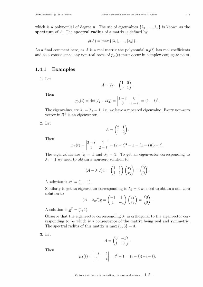


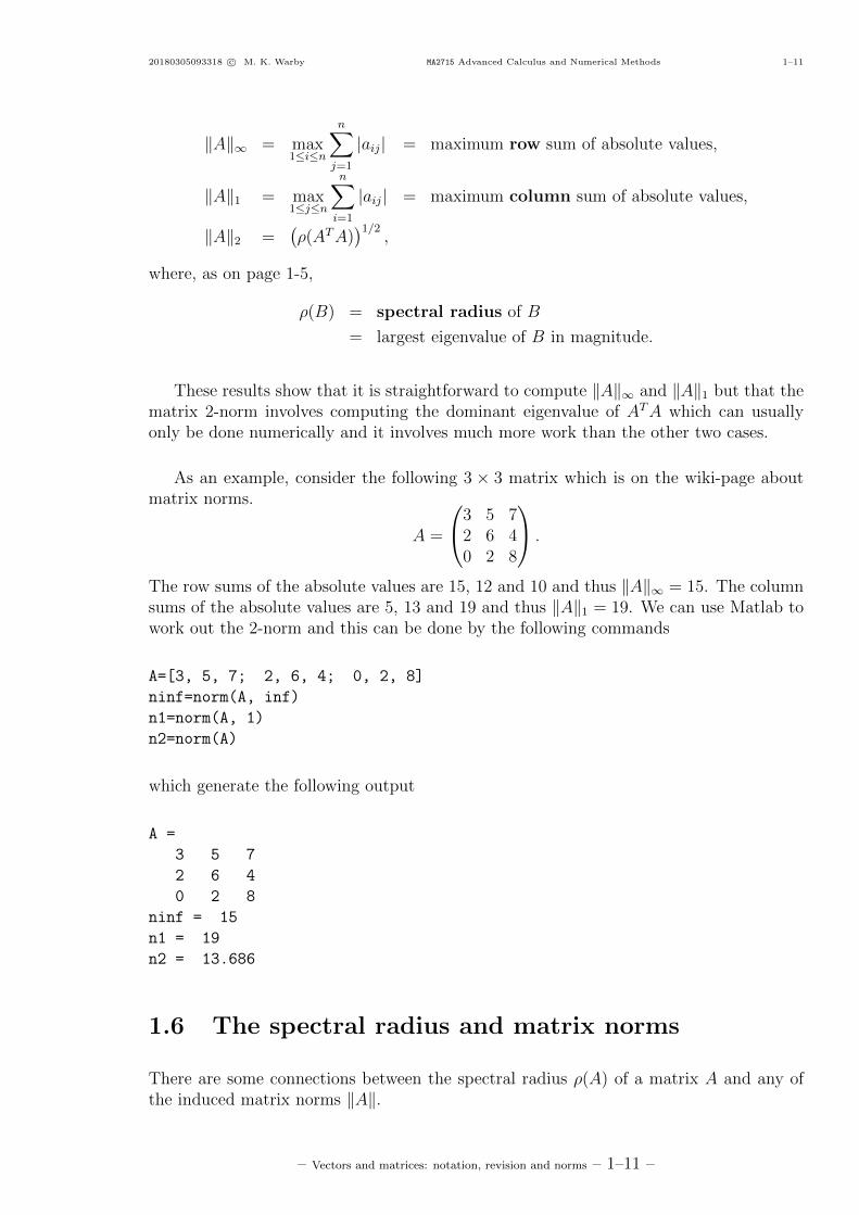


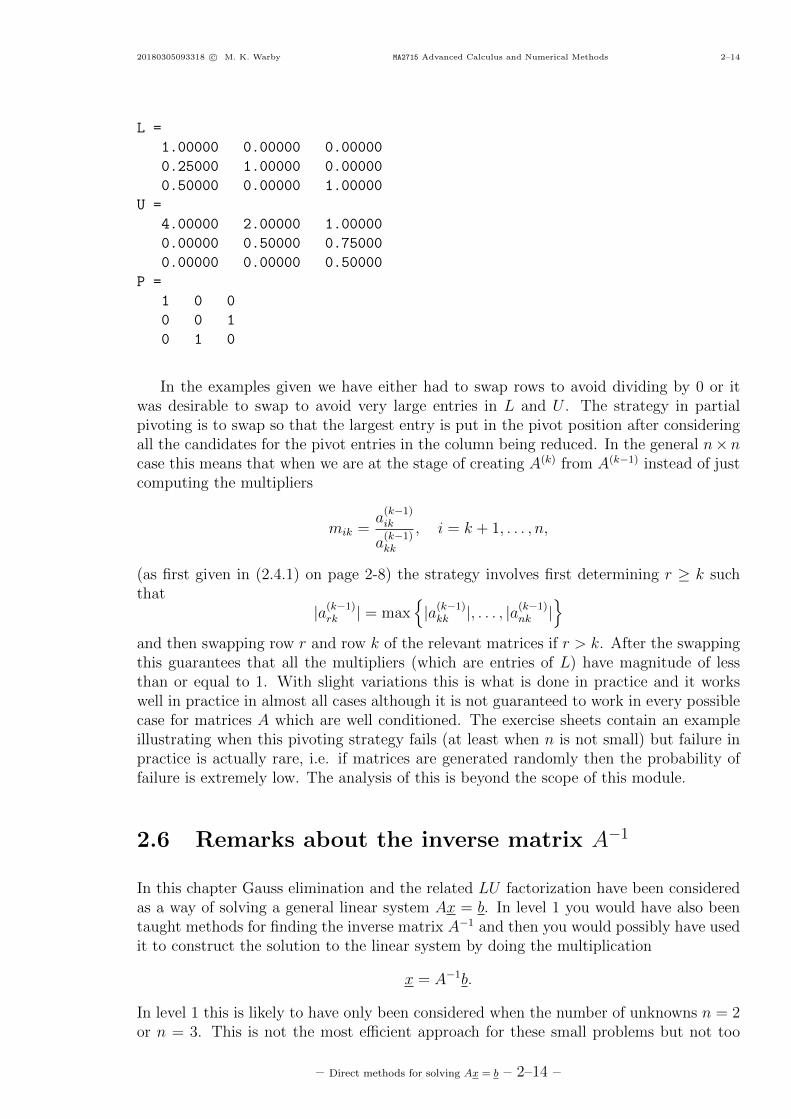


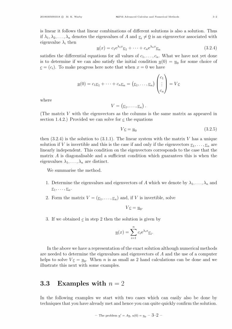
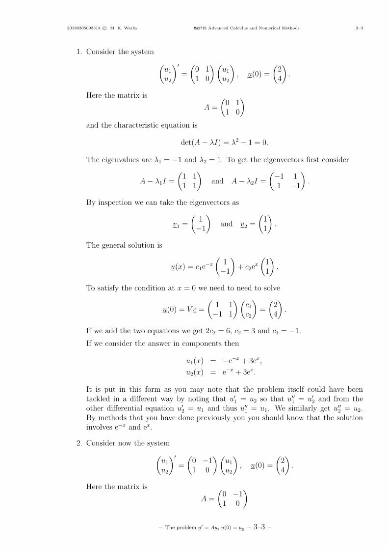


!["The Content & Branding Playbook," Warby Parker >> Tim Riley [COMMERCISM 2014]](https://static.documents.pub/doc/80x56/544f822daf7959ac338b456e/the-content-branding-playbook-warby-parker-tim-riley-commercism-2014.jpg)
