Combined radiocarbon and CO₂ flux measurements used to determine in situ chlorinated solvent mineralization rate Boyd, T. J., Montgomery, M. T., Cuenca, R. H., & Hagimoto, Y. (2015). Combined radiocarbon and CO₂ flux measurements used to determine in situ chlorinated solvent mineralization rate. Environmental Science: Processes & Impacts, 17(3), 683-692. doi:10.1039/c4em00514g 10.1039/c4em00514g Royal Society of Chemistry Version of Record http://cdss.library.oregonstate.edu/sa-termsofuse
Transcript
Combined radiocarbon and CO₂ flux measu rements used to determine in si tu ch lorinated so lvent mineralization rate
Boyd, T. J., Montgomery, M. T., Cuenca, R. H., & Hagimoto, Y. (2015). Combined radiocarbon and CO₂ flux measurements used to determine in situ chlorinated solvent mineralization rate. Environmental Science: Processes & Impacts, 17(3), 683-692. doi:10.1039/c4em00514g
arbon and CO2 fluxmeasurements used to determine in situchlorinated solvent mineralization rate†
T. J. Boyd,*a M. T. Montgomery,a R. H. Cuencab and Y. Hagimotob
A series of combined measurements was made at the Naval Air Station North Island (NASNI) Installation
Restoration Site 5, Unit 2 during July and August 2013. Combined measurements included CO2
respiration rate, CO2 radiocarbon content to estimate chlorinated hydrocarbon (CH) mineralization and a
zone of influence (ZOI) model. CO2 was collected continuously over 2 two-week periods by
recirculating monitoring well headspace gas through NaOH traps. A series of 12 wells in the main CH
plume zone and a background well with no known historical contamination were sampled. The
background well CO2 was used to determine radiocarbon content derived from respired natural organic
matter. A two end-member mixing model was then used to determine the amount of CH-derived
carbon present in the CO2 collected from plume region wells. The ZOI model provided an estimate for
the soil volume sampled at each well. CH mineralization rates were highest upgradient and at the plume
fringe for areas of high historical contamination and ranged from 0.02 to 5.6 mg CH carbon per day.
Using the ZOI model volume estimates, CH–carbon removal ranged from 0.2 to 32 mg CH–carbon m�3
per day. Because the rate estimates were based on a limited sampling (temporally), they were not further
extrapolated to long-term contaminant degradation estimates. However, if the site manager or
regulators required them, estimates – subject to long-term variability uncertainties – could be made
using volume and rate data determined over short timescales. A more comprehensive seasonal sampling
is needed to constrain long-term remediation models for the entire impacted area and identify
environmental conditions related to more rapid turnover times amongst the wells.
Environmental impact
CO2 radiocarbon analysis has proved extremely useful in denitively demonstrating on-site hydrocarbon (fuels, industrial chemicals, etc.) remediation to a non-toxic end-product. Vadoze-zone and groundwater CO2 which is radiocarbon-depleted relative to background CO2 conrms fossil-fuel or industrial chemicaldegradation. Combining CO2 radiocarbon analysis, on-site CO2 production rate, and a hydrogeologic Zone of Inuence (ZOI) model for each collection wellallows calculating contaminant degradation per unit time and unit area. Combining these measurements allows an environmental manager to estimate time-to-remediate for specic regions within a site – or the entire site. This information aids in evaluating remediation alternatives and can be used throughout the life-cycle of site analysis to assess remediation.
Introduction
The Department of Defense (DoD), Department of Energy(DOE), other federal agencies and civilian entities are faced withbillion dollar expenditures for environmental cleanup in theUnited States. Prohibitive cleanup costs make treatment
strategies such as monitored natural attenuation (MNA),enhanced passive remediation (EPR) or low cost engineeredsolutions attractive remediation alternatives for reachingResponse Complete (RC) status. Historically, lines ofconverging evidence are used to establish the occurrence of insitu bioremediation, abiotic contaminant conversion, or otherforms of natural attenuation. It is oen accepted that no singleanalysis or combination of ex situ laboratory tests provides anaccurate contaminant turnover conrmation or rate informa-tion for contaminant degradation under in situ conditions.1–4
Similarly, reports sponsored by DoD, DOE and EnvironmentalProtection Agency (EPA) advocate collection of a wide array ofdata to conrm contaminant attenuation and predict time-scale(s) for remediation.5–7
Multiple lines of evidence provide a means for rening whatoccurs on-site and in some instances, may provide indirectcontaminant degradation rate estimates. However, sitemanagers are under considerable pressure to decrease costswhile still obtaining the most realistic and complete siteconceptual model data. A clear need exists for relatively inex-pensive methods that are able to provide compelling evidencefor contaminant turnover while also offering realistic rate esti-mates for obtaining cleanup goals. Combining natural abun-dance 14CO2 measurements with CO2 production (contaminantrespiration) rates offers a method for simultaneously deter-mining the amount of CO2 generated from the contaminantpool and that CO2's generation rate (be it biodegradation orabiotic conversion).8
Because of the very distinct fossil carbon signatures (devoidof 14C) relative to contemporary carbon (modern), 14CO2 anal-ysis has recently been applied to tracking fossil fuel-derivedcontaminant degradation products.8–14 Analytical resolutionbetween the two end members (fossil and contemporary) is over1100 parts per thousand (standard measurement scale) and canbe accurately measured on contemporary AMS systems. Livingbiomass, atmospheric CO2, and soil organic matter-derived CO2
are all analytically distinct from fossil-derived CO2. Petroleumand petroleum-sourced industrial chemicals have a distinctradiocarbon signature (0% modern) and the absence of 14C isevenly distributed throughout the contaminant pool – offering abuilt-in tracer. As radioactive decay rates are unchanging, theonly potential bias in this measurement is toward the conser-vative (for example, if some atmospheric CO2 contaminates asample themeasurement will bemoremodern and thus will notoverestimate degradation rate).
If considerable degradation (contaminant oxidation) isoccurring, CO2 evolution associated with a fossil-fuel basedcontaminant plume will reect the carbon source. Up-gradientof the plume (e.g. background site), groundwater and soil CO2
will be primarily derived from respired natural organic matter.Within the plume or at the fringes, biodegrading contaminantwill generate CO2 with 0% modern carbon. This signal can bedifferentiated from CO2 from natural organic carbon sourcesusing a two end-member mixing model.12,13 With onemeasurement, it is possible to directly link contaminantdegradation to the on-site CO2 pool.
This single measurement technique, applied to several sites,has linked contaminant turnover to fossil-hydrocarbon orindustrial chemical oxidation.5–9 Although this singular analyt-ical method is powerful evidence that contaminants are beingdegraded to CO2 in situ, it does not readily allow calculatingcontaminant turnover rates without additional site informa-tion. It only denes what percentage of the total respiration CO2
pool is due to contaminant degradation relative to naturalorganic matter. A logical next step would be to couple CO2
source (contaminant versus natural organic matter) with CO2
production rate to estimate intrinsic contaminant biodegrada-tion rate. In previous studies, short-term soil respiration rateswere measured at the same site where soil gas CO2 radiocarbonanalysis indicated fossil fuel contributed signicantly to theCO2 pool.8 The data were scaled to the site's area such that a two
dimensional ux measurement for contaminant carbon couldbe estimated.
Many techniques exist for determining CO2 ux within soilhorizons. Generally, methods may have open- or closed-systemdesigns.15 Most recently, ux chambers (a type of closed-system)and gas ux models were used to estimate net respiration incontaminated soils.8,14,16,17 These techniques applied over arange of sub-sites (e.g. over a contaminant plume and back-ground areas) estimate increased CO2 production attributableto organic contaminants. Although the two-dimensional ux atthe air:soil interface can estimate contaminant turnover, itprovides only a net ux two-dimensional estimate (m2 per day).Scaling to 3-D required a soil ux model. Another means toobtain a 3-dimensional CO2 gas production rate is to trap CO2
from a “known” volume over unit time. This also requiresmodeling the system to determine the volume within thecollection sphere. Collecting CO2 from soil gas or groundwateris relatively easy and inexpensive, however, the ability toconrm that CO2 produced is denitively linked to thecontaminant on-site requires radiocarbon analysis – which maybe sample limited (�1 mg CO2 needed).
In this study, the goal was to collect CO2 produced at apredominately TCE-contaminated groundwater site over timeto both assess CH to CO2 conversion rates and synchronouslycollect ample CO2 for conrmatory radiocarbon analysis. Anadditional goal was to produce a ZOI model to calculate TCEconversion to CO2 on a per unit volume and per unit timebasis.
Materials and methodsSite description
IR Site 5, Unit 2 at North Island, CA (Fig. 1) was identied as aprime candidate to couple radiocarbon and CO2 uxmeasurements due to a rich archive of existing data oncontaminant levels, hydrogeology and the need for site closureinformation. The site is a former landll with an estimated2000 tons of hazardous wastes disposed at the site prior to1970. Waste was then transferred off-site. The area was con-verted to a golf course in 1983. Two pits were associated withUnit 2 (Eastern and Western). Only the Eastern pit was exca-vated (2001). Waste deposited at IR-5 included trash, solvents,oils, caustics, hydraulic uid, contaminated solid waste, sludgeand paints.
Current site activity includes monitoring, inspection andmaintenance of the landll cover. Within Unit 2, monitoringwas conducted semi-annually until mid-2008 and the plume ofchlorinated solvent material (in some wells over 1 g L�1)appears to be slowly receding over time. The presumedattenuation mechanism is biological degradation. Unit 2consists of mostly natural vegetation (Fig. 1). Wells within theadjacent IR Site 5 Unit 1 were sampled for dissolved CO2
radiocarbon when searching for a suitable background siteduring a previous study at NASNI and found to be relativelydepleted in 14C.13
The site is tted with numerous groundwater sampling wellsinstalled from 2000–2005, made from 40 0 PVC pipe and screened
Fig. 1 Sample site. Engineering diagram shows central well cluster.Sampled wells in green text.
Fig. 2 Well sampling schematic.
Paper Environmental Science: Processes & Impacts
Publ
ishe
d on
05
Febr
uary
201
5. D
ownl
oade
d by
Ore
gon
Stat
e U
nive
rsity
on
24/0
4/20
15 1
4:48
:31.
View Article Online
across the groundwater:vadose transition. It is seldomdisturbed being in the approach path to a runway. Twelve wellswithin a central cluster were used for CO2 collection. A back-ground well upgradient of any known contamination was usedfor background CO2 radiocarbon age and ux measurements.13
San Diego has a Mediterranean-like climate with two majorseasonal patterns (wet and dry season). The limited samplingevent described here was conducted during June and August2013 – during the dry season. Rain total prior to sampling was11.2 cm for the calendar 2013 year. At the site, historicalcontamination from chlorinated hydrocarbons was elevatedwithin the central well cluster (MW-25–MW-30) and on theNorthern portion of the site near Sherman Road (Fig. 1 – largestzoom). Contaminated soil was removed from the historicallandll site in 1983 and the Eastern waste pit of Unit 2 in 2001.Since that time, regular monitoring has revealed decreasing CHconcentrations with persistently high contamination at thecentral well cluster. According to site managers, seasonal rains(Dec–Feb) typically elute CHs off soils in the vadose zone whichtransiently increases groundwater CH concentrations.18 Soilshave been identied as primarily sands (from dredging opera-tions last century). No signicant sources of CaCO3 have beenidentied.
A CO2 collection system consisting of solar power cells, batterybanks, voltage controllers, sealed pumps, tubing, well caps, andNaOH traps was developed and deployed on-site. Battery-pow-ered pumps (Won Brothers LifeAir 50) were modied to intakeonly from a glued Teon tubing connection and output througha separate tube (1/1600). Tubing was glued into place using epoxyand sealed with silicone sealant. Battery powered pumps weremodied by the manufacturer to accept 3 V from a wiredconnection. Solar panels were used to recharge deep-cyclebatteries and appropriate step-down transformers were used todeliver �3 V to each pump. For the main well cluster and abackground well, a pump and associated sampling infrastruc-ture was installed. The sample cluster for pumps was limited towells within the range of the solar panel and wiring. Initialsamples (groundwater only) collected previous to pumpdeployment (March 2013) covered a larger area. It was notpossible given ight path restrictions and solar power require-ments to cover a wider sampling area for CO2 collection.
Sealable well caps (Dean Bennett Supply, Denver, CO) weremodied with thru-tubes to allow removal of gas from the wellheadspace and return CO2-scrubbed gas to the same headspace(thus producing no net “draw” from the well). The draw tubewas approximately 2 meters and pushed down toward – butabove – the groundwater level while the return tube extendedonly �10 cm from the well cap. A CO2 trap consisting of �50 gNaOH pellets was made from a 100 mL serum bottle and Teon-lined septum (Fig. 2).
Before CO2 was captured, each well pump was run for�48 hours (at least 60 well casing volumes) and trapped CO2 –
presumed to be a mixture of in-well CO2 and CO2 drawn in fromopening the well – was discarded. A fresh CO2 trap was installed
and pumps were run continuously for two 2 week periods (oneset of traps per 2 weeks). Traps were shipped to NRL forsubsequent analysis.
Pump operation was monitored using a voltage sensor foreach pump (Hobo U-12 data loggers, Onset, Bourne, MA).Pumps were generally operational for the full period, however,towards the end of each 2 week period, early morning operationbecame limited as solar cells could not keep up with theconstant current draw. Several pumps did not survive the full4 week collection period (dead motor, disintegrated plastic,etc.). These issues are addressed in the results section. Nouncompromised pumps were non-operational for more than 4 hduring any 24 h period.
CO2 production analysis
Serum bottle contents with trapped CO2 were carefully trans-ferred to a large graduated cylinder and diluted with puriedwater (MilliQ > 18 MU resistance) until all NaOH pellets weredissolved. Triplicate sub-samples from each 2 week collectionwere then transferred to 20 mL serum bottles. Samples wereappropriately diluted and analyzed by acidifying the CO2 out ofsolution and measuring by coulometry.19 CO2 was quantiedrelative to a certied reference material.20 Samples were run induplicate and values were averaged for reporting. Production(collection) rate was calculated dividing the total recovered CO2
by the time of collection (annotated for each well). Becausetrapping CO2 from the well headspace could introduce anequilibrium CO2 transfer from the adjacent volume to the wellhead-space, CO2 collection rates were converted to CO2
production rates by subtracting the average collection value forthe lowest value well (see Results section). The CO2 ux fromthis well was assumed to be solely driven by equilibrium (eventhough organic matter and contaminating mineralization mayhave occurred). CO2 collection and production rates were aver-aged between the two collection periods to obtain a represen-tative “dry season” values.
Radiocarbon analysis
CO2 trapped in aqueous NaOH (le over aer coulometricanalysis) was sent to Beta Analytic (Miami, FL) for radiocarbondating using accelerator mass spectrometry (AMS). Sampleswere also analyzed for d13CO2 ratios using methods previouslydescribed.13
Water quality analysis
In order to rule out any sources of potential CO2 contaminationwhich might bias radiocarbon measurements, cations poten-tially associated with carbonate dissolution, fertilizer use(potassium carbonates) and seawater intrusion were measured.Carbonate carbon could be ancient relative to background.Water samples were taken in pre-cleaned 40mL vials for pH andcation concentrations. Samples were assayed for K+, Ca++, Mg++
and Na+ ions using a Dionex DX120 ion chromatograph with aCS12A cation column as previously described.13 Stoichiometricdifferences between seawater and groundwater Na+ : Ca++ ratioscoupled with low pH relative to background wells were
evaluated as a potential indication of carbonate dissolution.Soil characterization data from borehole studies at two sites onNorth Island indicated no limestone soil lenses.
Zone of inuence model/simulation
A ZOI model was created based on well and local soil charac-teristics. These included well construction (casing dimensions,depth to water) temperature, atmospheric pressure and soilpermeability values. Analysis of well logs and prior well tests inthe project area was used to develop a hydrogeologic site model.This information was coupled with CO2 equilibrium simula-tions to create the ZOI model. The ZOI model was developedusing MT3DMS21 and MODFLOW-2005.22 MT3DMS is thebiodegradation model capable of simulating multi-solutetransport and reaction, and was used to simulate CO2 solutetransport as a part of the ZOI model. MODFLOW-2005 is thehydrogeological model considered as the reference code tosimulate groundwater dynamics and was used to simulategroundwater ow in the unconned aquifer at the study site.The two models have been used together as the standardpackage for multi-species contaminant transport simulations.23
In this study, ModelMuse linked and interfaced the twomodels.24
The study target was CO2 produced from chlorinatedsolvents (e.g. TCE and its breakdown products DCE and VC).Among different biodegradation models studied (e.g.MT3DMS,RT3D, Biosereen, Biochlor, and SEAM3D), a groundwatersimulation model and a complex CO2 transformation systemtracking CO2 solutes from different sources was needed. Mod-elMuse was able to adequately couple models for this purpose.Simulations treated all CO2 with different origins together –
radiocarbon content was then used to uniquely distinguish CO2
derived from chlorinated solvents.
Determining contaminant respired
Radiocarbon data were converted to D14C notation as neededfor further calculations using standard methods.25 An isotopicmixing model was applied to each sample using CO2 radio-carbon value collected at MW-01 as the site-wide backgroundvalue.12 MW-01 is roughly 400 meters northwest of the maincontamination. There is no known contamination at this well(planned background well). Background D14C was�162& (MW-01) and D14Cpetroleum was assigned the value �999&. Thefractionpetroleum was solved using eqn (1):
14C-content measurements were used to determine theproportion of vadose zone CO2 derived from contaminants ofinterest (CH).12 These values were then coupled with hydro-geologic model data to determine contaminant ux throughoxidation processes to CO2. The CO2 production rate at wellMW-01 was not used for this correction – only to calculatefraction petroleum. Comparing in-plume measurements withreference site(s) measurements allowed source apportioning in
a Based on single 2 week collection (pump failure). b Modern value(1950+) – indicated pump leak. c Assumed to be purely equilibrium-driven.
Results and discussionCation and pH analysis
Samples for cation and pH were analyzed for March 2013 andJuly 2013 samplings. pH was near neutral for most wells exceptfor MW-01 (background) and MW-38 (Table 1). Wells on thesite's Southern side generally had a higher Na+ content, butwere not in a range which indicated signicant seawaterintrusion. pH was elevated in the pre-sampling (March 2013 –
see ESI†), but cation concentrations were not signicantlydifferent. We speculate seasonal rains (typically Januarythrough March) impact groundwater pH. Calcium ion concen-trations ranged from 8.0 to 66 mg L�1 (Table 1) but did notinversely correlate with pH to indicate signicant carbonatedissolution during either sampling (r2 < 0.3). We performed atrend analysis with the water quality data using principalcomponents analysis (PCA). Bi-plots showed no strong loadingswith any variable (Ca2+ being of most concern). We thusassumed any possible interferences were minimal and would beencapsulated within the background well's radiocarbon ratio(s).
CO2 collection and production rates
CO2 collection rates ranged from 0 (see equilibrium subtractionbelow) to 34 mg CO2 per day (Table 2). CO2 collection was lowestin the central well cluster where historical contamination washighest. Because CO2 was constantly scrubbed from the wellcasing, a physical equilibrium-driven “draw” of CO2 shouldhave occurred in each well (in addition to CO2 driven into thewell headspace due to active respiration). There was no corre-lation between the dissolved CO2 in the groundwater collectedimmediately before the wells were sealed and pumping started(data in ESI†). The lowest collection rate (MW-25) was used toestimate the CO2 trapped only from physical equilibriumkinetics. This well coincidentally also had CO2 with the youn-gest radiocarbon age relative to the background well (Table 2).The collection rate at this well was conservatively estimated as
Table 1 Water quality parameter for July 2013 sampling
the physical CO2 equilibrium inuence and was subtracted (asproportion of starting DIC � raw CO2 collection � (DIC �MW-25 collection rate/MW-25 DIC)) from all other collectionrates to calculate CO2 production rate in each well. MW-01(background well) had high CO2 production rate at�31 mg CO2
per day. Standard error for duplicate analyses averaged 0.98%and ranged from 0.03 to 4%. Two 2 week periods were sampledduring the same season and averaged for subsequent calcula-tions (e.g. preliminary time-to-remediate). Standard error forCO2 ranged from <1 to 51% between the two collection periods.However, most standard errors were relatively low and averaged�13% (Table 2). While introducing additional error, averagingallowed a single calculation for volume removed during a onemonth period.
CO2 carbon isotope analysis
Twenty six NaOH-trapped CO2 samples were analyzed forradiocarbon. Two wells (MW-27 and MW-32) had pump issues(became unsealed allowing atmospheric CO2 intrusion) andwere suspect but sent for analysis anyway. Stable carbon isotoperatios for CO2 indicated potential contamination with atmo-spheric CO2 (typically �7&VPDB) for MW-27. MW-32, which alsoleaked at the inlet line, had a d13CO2 value similar to other wells.d13CO2 values were in a range to indicate respiration fromnatural organic matter sources (Table 2). Many values werelighter than ��25&VPDB. This might indicate removal ofisotopically-lighter contaminant source or daughter products.In a previous studies, several wells were sampled for compound-specic stable carbon isotope values (MW-21, MW-41, MW-42,and MW-43). In wells where cis-1,2-DCE concentrationsdecreased between the two time-points studied (about 1 yearapart), there was a concomitant 13C enrichment in theremaining cis-1,2-DCE pool.
The background well (MW-01) had a D14C ratio of �147&.This equates to 1280 years before present (ybp) or 85% modern
(pMC). This well was used as the background for the isotopicmixing model. Radiocarbon ratios ranged from �147& to�663& at the fringe of the removed source area (ShermanRoad) with wells near the central cluster of high residualcontamination showing relatively modern values (e.g. close to0 – Table 2). As with CO2 production, the two sampling periodsamples were averaged for subsequent calculations. Radio-carbon ratio measurements were very similar between indi-vidual 2 week periods. Standard error between periods averaged6% and ranged from 0.25 to 18%.
ZOI model
Groundwater hydraulic and CO2 solute properties for the studysite were obtained from previous reports.26,27 Three years ofweather data (2007, 2011 and 2012) were obtained from CIMISSan Diego station (Station ID 184) to estimate aquifer rechargerate. Tidal data for the same three years were obtained from theNOAA San Diego Station (Station ID: 9410170) to deneboundary conditions. From the aerial photo, surface waterpools (e.g. ponds and creeks) were identied adjacent to the site(in the golf course and park). A constant head equal to theelevation of these surface water bodies was assigned to theboundary.
The areal model indicated that the effects of short term (dailyand weekly periods) changes in sea level around the peninsulaon groundwater ow at the study site were insignicant. Thisagrees with the previous reports18 and cation analysis presentedhere. Groundwater hydrology at the study site is usually steadybetween late summer and fall, therefore, ow during CO2
collection (July–August 2013) was assumed steady (i.e. constanthydraulic gradient). The hydraulic gradient estimated by theareal model was 0.009 m m�1, which was reasonably close tothat estimated from the groundwater elevation map in June2011.26 Other parameters were obtained from the literature(Table 3).
Initial solute CO2 distribution in the aquifer around thesampling well was assumed in equilibrium with the CO2
supplied from overlying soil gas and mineralization; therefore,
Table 3 Parameter summary for ZOI model
Parameter Units Value
HydrologyHydraulic conductivity mL h�1 0.44 (aquifer) 10 (well)Porosity (aquifer) 0.48 (aquifer) 0.99 (well)Bulk density g cm�3 1.4Specic yield cm3 cm�3 0.2Hydraulic gradient m m�1 0.015
CO2 solute transportDiffusion coefficient m2 h�1 5.77 � 10�5
Longitudinal dispersivity m 6.1Horizontal transversedispersivity
CO2 distribution was assumed uniform. Any CO2 gradientobserved at the end of the 2 week simulation period wasassumed to be attributable to CO2 collection in the well. Withuniform CO2 distribution, the ZOI associated with CO2 collec-tion was dened as the volume of aquifer that had a CO2
concentration 95% or less of the initial concentration. UsingHenry's law, CO2 equilibrium concentration at the groundwatertable with the CO2-rich soil gas was estimated as 8.4 g CO2 m
�3.Because biochemical conditions in the unconned aquiferduring CO2 collection was unknown, the ZOI model assumedconstant mineralization rates for chlorinated solvents (e.g. DCEand VC half lives ¼ 3.8 and 9.5 years, respectively). The ZOImodel was thus simplied by not accounting for mineralizationduring the 2 week CO2 collection period. However, mineraliza-tion has certainly accumulated CO2 in the aquifer over time asCO2 radiocarbon ages were older than background (Table 4).
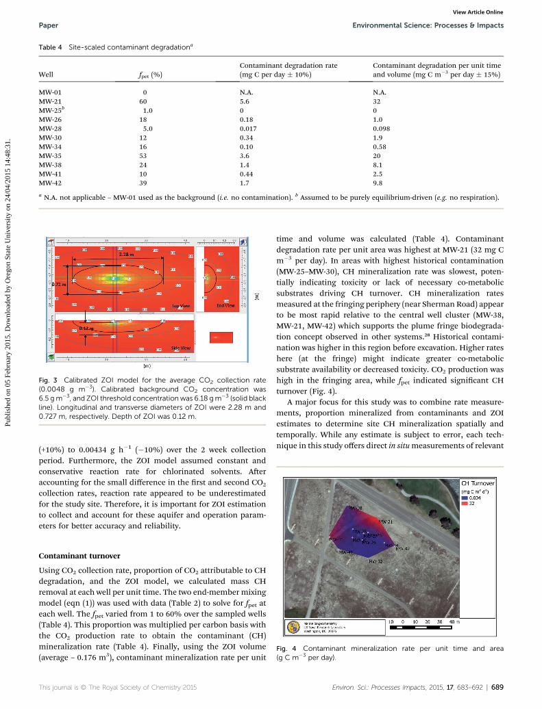
The calibrated ZOI model was run with the estimatedhydraulic gradient (0.015 m m�1) and hypothetical backgroundCO2 concentration (8.4 g CO2 m�3). The entire model domainfor this scenario was 9.0 m � 4.5 m � 10.0 m deep. Horizontalspatial resolution was set to 0.09 m � 0.09 m, which makes onegrid area equal to 0.0081 m2, the same as the well area. Verticalspatial resolution varied from 0.05 m at the surface to 1.7 m atthe bottom. The hydraulic gradient was applied to the ZOImodel by setting the constant head condition along twoboundaries allowing groundwater to ow le to right (Fig. 3).
The ZOI model described above was then coupled withmeasured CO2 collection rates. Calibration assumed thatcollection rate was constant during the collection period. Cali-bration also assumed an equilibrium between CO2 output (i.e.collection) and supply (i.e. diffusion) at the well water table. Inother words, CO2 concentration at the well water surface wasassumed to decrease to 0.0 g CO2 m�3 by the end of thesimulation.
ZOI calibration varied when taking CO2 collection rate intoaccount. Measured collection rate linearly correlated with thecalibrated background CO2 groundwater concentration (r2 ¼0.96). Also, estimated ZOI volume was linearly correlated withbackground CO2 concentration (r2 ¼ 0.98) and thus CO2
collection rate. Assuming 0.04% partial pressure of atmosphericCO2, equilibrium CO2 concentration of non-contaminatedaquifer exposed to the atmosphere would be 0.60 g m�3. Esti-mated background CO2 concentration for all collection rateswas higher than this value suggesting groundwater contami-nation with chlorinated solvents (e.g. TCE, DCE, VC) and theiractive mineralization. However, estimated background CO2
concentrations are below solubility of CO2 (1450 g m�3 at 25 �C)and do not indicate CO2 saturation in the aquifer.
The calibration assumes a steady hydraulic gradient andconstant collection rates. A supplemental simulation foraverage CO2 collection rate indicated approximately 50%increase in estimated background CO2 concentration (i.e.increased from 6.5 to 9.7 g m�3) with 10% increase in hydraulicgradient (i.e. increased from 0.0150 to 0.0165 m m�1). Anothersupplemental simulation for average CO2 production rateincreased background CO2 concentration by 46% (i.e. increased6.5 to 9.5 g m�3) if the collection rate changed from 0.00530
a N.A. not applicable – MW-01 used as the background (i.e. no contamination). b Assumed to be purely equilibrium-driven (e.g. no respiration).
Fig. 3 Calibrated ZOI model for the average CO2 collection rate(0.0048 g m�3). Calibrated background CO2 concentration was6.5 gm�3, and ZOI threshold concentration was 6.18 gm�3 (solid blackline). Longitudinal and transverse diameters of ZOI were 2.28 m and0.727 m, respectively. Depth of ZOI was 0.12 m.
Paper Environmental Science: Processes & Impacts
Publ
ishe
d on
05
Febr
uary
201
5. D
ownl
oade
d by
Ore
gon
Stat
e U
nive
rsity
on
24/0
4/20
15 1
4:48
:31.
View Article Online
(+10%) to 0.00434 g h�1 (�10%) over the 2 week collectionperiod. Furthermore, the ZOI model assumed constant andconservative reaction rate for chlorinated solvents. Aeraccounting for the small difference in the rst and second CO2
collection rates, reaction rate appeared to be underestimatedfor the study site. Therefore, it is important for ZOI estimationto collect and account for these aquifer and operation param-eters for better accuracy and reliability.
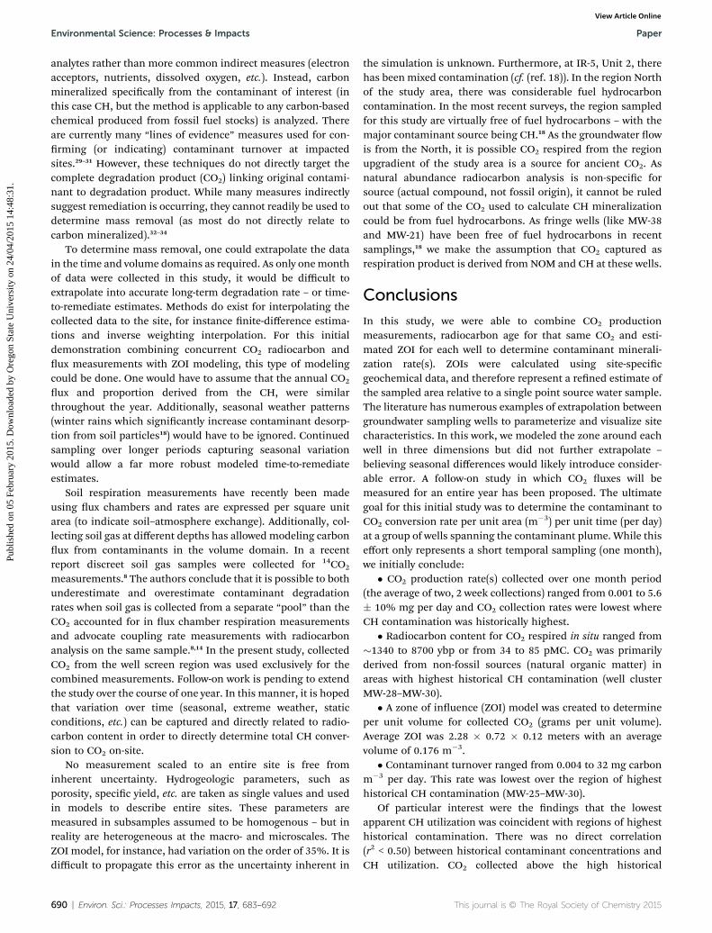
Fig. 4 Contaminant mineralization rate per unit time and area(g C m�3 per day).
Contaminant turnover
Using CO2 collection rate, proportion of CO2 attributable to CHdegradation, and the ZOI model, we calculated mass CHremoval at each well per unit time. The two end-member mixingmodel (eqn (1)) was used with data (Table 2) to solve for fpet ateach well. The fpet varied from 1 to 60% over the sampled wells(Table 4). This proportion was multiplied per carbon basis withthe CO2 production rate to obtain the contaminant (CH)mineralization rate (Table 4). Finally, using the ZOI volume(average – 0.176 m3), contaminant mineralization rate per unit
time and volume was calculated (Table 4). Contaminantdegradation rate per unit area was highest at MW-21 (32 mg Cm�3 per day). In areas with highest historical contamination(MW-25–MW-30), CH mineralization rate was slowest, poten-tially indicating toxicity or lack of necessary co-metabolicsubstrates driving CH turnover. CH mineralization ratesmeasured at the fringing periphery (near Sherman Road) appearto be most rapid relative to the central well cluster (MW-38,MW-21, MW-42) which supports the plume fringe biodegrada-tion concept observed in other systems.28 Historical contami-nation was higher in this region before excavation. Higher rateshere (at the fringe) might indicate greater co-metabolicsubstrate availability or decreased toxicity. CO2 production washigh in the fringing area, while fpet indicated signicant CHturnover (Fig. 4).
A major focus for this study was to combine rate measure-ments, proportion mineralized from contaminants and ZOIestimates to determine site CH mineralization spatially andtemporally. While any estimate is subject to error, each tech-nique in this study offers direct in situmeasurements of relevant
analytes rather than more common indirect measures (electronacceptors, nutrients, dissolved oxygen, etc.). Instead, carbonmineralized specically from the contaminant of interest (inthis case CH, but the method is applicable to any carbon-basedchemical produced from fossil fuel stocks) is analyzed. Thereare currently many “lines of evidence” measures used for con-rming (or indicating) contaminant turnover at impactedsites.29–31 However, these techniques do not directly target thecomplete degradation product (CO2) linking original contami-nant to degradation product. While many measures indirectlysuggest remediation is occurring, they cannot readily be used todetermine mass removal (as most do not directly relate tocarbon mineralized).32–34
To determine mass removal, one could extrapolate the datain the time and volume domains as required. As only onemonthof data were collected in this study, it would be difficult toextrapolate into accurate long-term degradation rate – or time-to-remediate estimates. Methods do exist for interpolating thecollected data to the site, for instance nite-difference estima-tions and inverse weighting interpolation. For this initialdemonstration combining concurrent CO2 radiocarbon andux measurements with ZOI modeling, this type of modelingcould be done. One would have to assume that the annual CO2
ux and proportion derived from the CH, were similarthroughout the year. Additionally, seasonal weather patterns(winter rains which signicantly increase contaminant desorp-tion from soil particles18) would have to be ignored. Continuedsampling over longer periods capturing seasonal variationwould allow a far more robust modeled time-to-remediateestimates.
Soil respiration measurements have recently been madeusing ux chambers and rates are expressed per square unitarea (to indicate soil–atmosphere exchange). Additionally, col-lecting soil gas at different depths has allowed modeling carbonux from contaminants in the volume domain. In a recentreport discreet soil gas samples were collected for 14CO2
measurements.8 The authors conclude that it is possible to bothunderestimate and overestimate contaminant degradationrates when soil gas is collected from a separate “pool” than theCO2 accounted for in ux chamber respiration measurementsand advocate coupling rate measurements with radiocarbonanalysis on the same sample.8,14 In the present study, collectedCO2 from the well screen region was used exclusively for thecombined measurements. Follow-on work is pending to extendthe study over the course of one year. In this manner, it is hopedthat variation over time (seasonal, extreme weather, staticconditions, etc.) can be captured and directly related to radio-carbon content in order to directly determine total CH conver-sion to CO2 on-site.
No measurement scaled to an entire site is free frominherent uncertainty. Hydrogeologic parameters, such asporosity, specic yield, etc. are taken as single values and usedin models to describe entire sites. These parameters aremeasured in subsamples assumed to be homogenous – but inreality are heterogeneous at the macro- and microscales. TheZOI model, for instance, had variation on the order of 35%. It isdifficult to propagate this error as the uncertainty inherent in
the simulation is unknown. Furthermore, at IR-5, Unit 2, therehas beenmixed contamination (cf. (ref. 18)). In the region Northof the study area, there was considerable fuel hydrocarboncontamination. In the most recent surveys, the region sampledfor this study are virtually free of fuel hydrocarbons – with themajor contaminant source being CH.18 As the groundwater owis from the North, it is possible CO2 respired from the regionupgradient of the study area is a source for ancient CO2. Asnatural abundance radiocarbon analysis is non-specic forsource (actual compound, not fossil origin), it cannot be ruledout that some of the CO2 used to calculate CH mineralizationcould be from fuel hydrocarbons. As fringe wells (like MW-38and MW-21) have been free of fuel hydrocarbons in recentsamplings,18 we make the assumption that CO2 captured asrespiration product is derived from NOM and CH at these wells.
Conclusions
In this study, we were able to combine CO2 productionmeasurements, radiocarbon age for that same CO2 and esti-mated ZOI for each well to determine contaminant minerali-zation rate(s). ZOIs were calculated using site-specicgeochemical data, and therefore represent a rened estimate ofthe sampled area relative to a single point source water sample.The literature has numerous examples of extrapolation betweengroundwater sampling wells to parameterize and visualize sitecharacteristics. In this work, we modeled the zone around eachwell in three dimensions but did not further extrapolate –
believing seasonal differences would likely introduce consider-able error. A follow-on study in which CO2 uxes will bemeasured for an entire year has been proposed. The ultimategoal for this initial study was to determine the contaminant toCO2 conversion rate per unit area (m�3) per unit time (per day)at a group of wells spanning the contaminant plume. While thiseffort only represents a short temporal sampling (one month),we initially conclude:
� CO2 production rate(s) collected over one month period(the average of two, 2 week collections) ranged from 0.001 to 5.6� 10% mg per day and CO2 collection rates were lowest whereCH contamination was historically highest.
� Radiocarbon content for CO2 respired in situ ranged from�1340 to 8700 ybp or from 34 to 85 pMC. CO2 was primarilyderived from non-fossil sources (natural organic matter) inareas with highest historical CH contamination (well clusterMW-28–MW-30).
� A zone of inuence (ZOI) model was created to determineper unit volume for collected CO2 (grams per unit volume).Average ZOI was 2.28 � 0.72 � 0.12 meters with an averagevolume of 0.176 m�3.
� Contaminant turnover ranged from 0.004 to 32 mg carbonm�3 per day. This rate was lowest over the region of highesthistorical CH contamination (MW-25–MW-30).
Of particular interest were the ndings that the lowestapparent CH utilization was coincident with regions of highesthistorical contamination. There was no direct correlation(r2 < 0.50) between historical contaminant concentrations andCH utilization. CO2 collected above the high historical
contamination region had the highest pMC indicating lessrelative contribution from CH than natural organic matter tothe relatively small respiration CO2 pool. This nding wascontrary to the previous study at NASNI in which the contami-nation was fuel hydrocarbons and CO2 collected within the fuelplume was distinctly from the fossil end-member.13 At present,it is unknown why CH conversion appears lowest where substrateconcentrations are highest. The plume fringe concept has becomewidely accepted (cf. (ref. 28)) as a model for this phenomenon. Wespeculate lack of cometabolic substrates coupled with the factthat CH degradation is usually a co-metabolic process (notoffering direct carbon and energy gains to the assemblage) aslikely reasons. Processes that spatially enhance the plume fringe(e.g. uctuating water table) may be important to increasingcontaminant mineralization rates at these types of sites. Forinstance, during rain events, nutrients, electron acceptors, andadditional substrates may be “released” into the groundwater.
Future research to advance this combined methodology andexpand the scope will focus on the present site to expand season-ality and rene the spatial approach by scaling well measurementsto individual well ZOIs. The approach is particularly appropriatefor sites where engineering approaches are in place (zero valentiron curtains, addition of electron acceptors, chemical oxidationadditions, etc.). Future planned activities at this site include:
� Additional seasonal samplings (currently planning sub-sampling every two weeks to gather “wet” and “dry” season totalCO2 production)
� Deploy more robust pumps (non-mechanical). While thepumps utilized in this study worked well in the laboratory forextended periods, they were not robust enough for eld use.Magnetic oscillating pumps, while drawing more power, havebeen procured for additional temporal sampling.
� Rene ZOI model by collecting and calibrating CO2
collection rates with groundwater concentrations.� Sample during, or, at least under the inuence of rain
events.� Given estimates of source size (kg), rene time to degrade
estimates.
Acknowledgements
Financial support for this research was provided by the StrategicEnvironmental Research and Development Program (SERDPER-2338; Andrea Leeson, Program Manager). Michael Pound,Naval Facilities Engineering Command, Southwest providedlogistical and site support for the project. Brian White, ErikaThompson and Richard Wong (CBI Federal Services, Inc)provided on-site logistical support, historical site perspectiveand relevant reports. Todd Wiedemeier (T. H. Wiedemeier &Associates) provided documentation, discussion and historicalsite perspectives.
Notes and references
1 National Research Council, In situ bioremediation: When doesit work?, National Academy of Sciences, Washington, DC,1993.
2 J. V. Weiss and I. M. Cozzarelli, Ground water, 2008, 46, 305–322.
3 W. A. Illman and P. J. Alvarez, Crit. Rev. Environ. Sci. Technol.,2009, 39, 209–270.
4 P. Bombach, H. H. Richnow, M. Kastner and A. Fischer, Appl.Microbiol. Biotechnol., 2010, 86, 839–852.
5 K. M. Vangelas, Summary Document of Workshops for Hanford,Oak Ridge and Savannah River Site as part of the MonitoredNatural Attenuation and Enhanced Passive Remediation forChlorinated Solvents – DOE Alternative Project for TechnologyAcceleration, U.S. Department of Energy, WestinghouseSavannah River Company, Aiken, SC, 2003.
6 T. H. Wiedemeier, M. A. Swanson, D. E. Moutoux,E. K. Gordon, J. T. Wilson, B. H. Wilson, D. H. Kampbell,P. E. Hass, R. N. Miller, J. E. Hansen and F. H. Chapelle,Technical Protocol for Evaluating Natural Attenuation ofChlorinated Solvents in Ground Water, USEPA Office ofResearch and Development, Washington, DC, 1998.
7 J. T. Wilson, D. H. Kampbell, M. Ferrey and P. Estuestra,Evaluation of the Protocol for Natural Attenuation ofChlorinated Solvents: Case Study at the Twin Cities ArmyAmmunition Plant, USEPA Office of Research andDevelopment, Washington, DC, 2001.
8 N. J. Sihota and K. Ulrich Mayer, Vadose Zone J., 2012, 11,DOI: 10.2136/vzj2011.0204.
9 C. M. Aelion, B. C. Kirtland and P. A. Stone, Environ. Sci.Technol., 1997, 31, 3363–3370.
10 B. C. Kirtland, C. M. Aelion, P. A. Stone and D. Hunkeler,Environ. Sci. Technol., 2003, 37, 4205–4212.
11 B. C. Kirtland, C. M. Aelion and P. A. Stone, J. Contam.Hydrol., 2005, 76, 1–18.
12 R. B. Coffin, J. W. Pohlman, K. S. Grabowski, D. L. Knies,R. E. Plummer, R. W. Magee and T. J. Boyd, Environ.Forensics, 2008, 9, 75–84.
13 T. J. Boyd, M. J. Pound, D. Lohr and R. B. Coffin, Environ. Sci.:Processes Impacts, 2013, 15, 912–918.
14 N. I. Sihota, O. Singurindy and K. U. Mayer, Environ. Sci.Technol., 2011, 45, 482–488.
15 J. M. Norman, C. J. Kucharik, S. T. Gower, D. D. Baldocchi,P. M. Crill, M. Rayment, K. Savage and R. G. Striegl, J.Geophys. Res., 1997, 102, 28771–28777.
16 R. T. Amos, K. U. Mayer, B. A. Bekins, G. N. Delin andR. L. Williams, Water Resour. Res., 2005, 41, 1–15.
17 S. Molins, K. U. Mayer, R. T. Amos and B. A. Bekins, J.Contam. Hydrol., 2010, 112, 15–29.
18 Shaw Infrastructure Inc., Dra Feasibility Study, InstallationRestoration Site 5, Unit 2, Naval Air Station North Island, SanDiego, California SHAW-4302-0075-2318, ShawInfrastructure, Inc, Concord, CA, 2013.
19 K. M. Johnson, J. M. Sieburth, P. J. l. B. Williams andL. Brandstrom, Mar. Chem., 1987, 21, 117–133.
20 A. G. Dickson, Oceanography, 2010, 23, 34–47.21 C. Zheng and P. P. Wang, MT3DMS: A modular three-
dimensional multispecies transport model for simulation ofadvection, dispersion, and chemical reactions of contaminantsin groundwater systems; documentation and user's guide,DTIC Document, 1999.
22 A. W. Harbaugh, MODFLOW-2005, the US Geological Surveymodular ground-water model: The ground-water ow process,US Department of the Interior, US Geological Survey, 2005.
23 H. Prommer, D. A. Barry and C. Zheng, Ground Water, 2003,41, 247–257.
24 R. B. Winston, in Ground Water-Book 6, U.S. GeologicalSurvey, Reston, VA, Editon edn, 2009, vol. Techniques andMethods 6–A29.
25 M. Stuiver and H. A. Polach, Radiocarbon, 1977, 19, 355–363.26 Accord Engineering Inc, Semi-Annual Post-Closure
Maintenance Report for Calendar Year 2011 InstallationRestoration (IR) Program Site 2 (Old Spanish Bight Landll),Site 4 (Public Works Salvage Yard), and Site 5, Unit 1 (GolfCourse Landll), San Diego, CA, 2011.
27 Geosyntec Consultants, Annual Progress Report October 2010to December 2011, Operable Unit 24, Columbia, MD, 2012.
28 R. D. Bauer, M. Rolle, S. Bauer, C. Eberhardt, P. Grathwohl,O. Kolditz, R. U. Meckenstock and C. Griebler, J. Contam.Hydrol., 2009, 105, 56–68.