C riminal incident prediction using a point-pattern … riminal incident prediction using a...

International Journal of Forecasting 19 (2003) 603–622www.elsevier.com/ locate/ ijforecast

C riminal incident prediction using a point-pattern-based densitymodel

a ,b*Hua Liu , Donald E. BrownaCSG Systems, Inc., One Main Street, Cambridge, MA 02142,USA

bDepartment of Systems and Information Engineering, University of Virginia, Charlottesville, VA 22903,USA

Abstract

Law enforcement agencies need crime forecasts to support their tactical operations; namely, predicted crime locations for next week basedon data from the previous week. Current practice simply assumes that spatial clusters of crimes or ‘‘hot spots’’ observed in the previousweek will persist to the next week. This paper introduces a multivariate prediction model for hot spots that relates the features in an area tothe predicted occurrence of crimes through the preference structure of criminals. We use a point-pattern-based transition density model forspace–time event prediction that relies on criminal preference discovery as observed in the features chosen for past crimes. The resultantmodel outperforms the current practices, as demonstrated statistically by an application to breaking and entering incidents in Richmond,VA. 2003 International Institute of Forecasters. Published by Elsevier B.V. All rights reserved.

Keywords: Point-pattern methods; Crime forecasting; Spatial transition density model; Hot spot prediction model

1 . Introduction crimes. Police assume that current crime clusters willpersist over the forecast horizon. A widely used such

Law enforcement agencies have a continuing need method is the Spatial and Temporal Analysis ofto predict the locations of crimes. Armed with Crime program (STAC) which clusters crime pointscriminal event predictions, police can target patrols, within ellipses(Block, 1995). Jefferis (1998)surveysdirect surveillance, and conduct other operations to additional hotspot methods, the most sophisticated ofprevent crimes and enforce laws. These activities which employ kernel density estimation(Levine,have horizons of days and, at most, weeks. 1998).

It is well known that crimes tend to cluster This paper extends crime clustering methods byspatially in so-called hot spots; for example, due to incorporating offenders’ preferences in crime sitecertain crime-prone land uses (e.g., convenience selection. A number of researchers have investigatedstores or bars) or established patterns of serial spatial decision making by criminals(Amir, 1971;criminals. Thus, the prevalent approach to forecast- Baldwin & Bottoms, 1976; Brantingham & Brantin-ing by police is a simple spatial clustering method gham, 1975, 1984; Capone & Nichols, 1976;using only the coordinates, dates, and types of LeBeau, 1987; Molumby, 1976; Newman, 1972;

Repetto, 1974; Rossmo, 1993, 1996; Scarr, 1973).Taken together, this body of research suggests that*Corresponding author. Tel.:11-434-982-2074.the likelihood of a criminal incident at a specifiedE-mail addresses: hua [email protected] (H. Liu),

][email protected](D.E. Brown). location is based on past incidents of the same type

0169-2070/03/$ – see front matter 2003 International Institute of Forecasters. Published by Elsevier B.V. All rights reserved.doi:10.1016/S0169-2070(03)00094-3

mailto:[email protected]




604 H. Liu, D.E. Brown / International Journal of Forecasting 19 (2003) 603–622

and independent spatial attributes or features (e.g. ships between demographic, economic, social, vic-distance to a road, type of residential community, tim, and spatial attributes and measures of criminaletc.). activity. The model represents a declining or rising

To formally describe the forecast problem, we trend as a decreasing or increasing likelihood ofdenote the locations and times of criminal incidents being victimized by crime. Furthermore, the modelas (s , t ), (s , t ), . . . , t 50, t , t , . . . , where can identify new potential hot spots or areas at risk1 1 2 2 0 1 2

s is the two-dimensional location of incidenti of a that are not necessarily in the vicinity of existingi

given crime type andt is the corresponding time. crime locations.i

Suppose that there arep measurable featuresf , In Section 2, we give an overview of our model1

f , . . . , f that are believed to be relevant to the specification process, and then discuss a Gini-index-2 p

occurrence of the incidents, with values consisting of based measure of cohesiveness for feature selection.p-dimensional vectorsx , x , . . . . Taken together, In Section 3, we present a model of the transition1 2

the locations, times, and features of all incidents are density as our approach for spatio-temporal eventa realization of a marked space–time shock point prediction. We also describe a comparison model inprocesshx [ x : s[D, t [ T j, where t, s, and x that section. In Section 4, we calibrate our proposeds,t s,t

are all random quantities confined within a study model on crime data from Richmond, VA, and1horizonT ,R , a study region or geographic space compare it to the current hot spot approach. Included

2 pD ,R , and a feature spacex ,R , respectively. are two sets of hypothesis tests. We briefly concludeThe space–time point process is marked by the in Section 5.feature vectors, and is a shock process because theevents of the process are considered instantaneous,as opposed to a survival process(Cressie, 1993). 2 . Model search method

The quantity of interest is the density of theprocess, which formally captures the likelihood that Our objective is to find the smallest feature subseta future criminal incident occurs within a study (of the initial feature set) that accounts for theregion and a study horizon, given the times, loca- underlying pattern of criminal event occurrences (hottions, and feature values of past incidents of the spots). This is a model search problem we callsame type bounded by the same region and time feature selection. The selected feature subset isrange. LetT 5 ht , t , . . . , t j, D 5 hs , s , . . . , s j, called the key feature set and the feature subspacen 1 2 n n 1 2 n

and x 5 hx , x , . . . , x j where s 5 (s , s ) and defined by the key feature set the key feature space.n 1 2 n i i1 i2

x 5 [x ? ? ? x ]9. The transition density is defined A feature selection problem is specified by ai i1 ip

as follows: triplet (F, c, s), whereF is the initial feature set,c acriterion function defined for subsets ofF, and s a

c (s ,t uD ,T ,x )n n11 n11 n n n subset search or selection procedure. For the selec-PrhN(ds ,dt )5 1uD ,T ,x j tion procedure, oftentimes we can just compare then11 n11 n n n]]]]]]]]]; lim scores of individual features and rank them accord-n(ds )dtn (ds ),dt →0n11 n11 n11 n11

ingly. This is feature ranking and will be the(1)approach that we use for our application in Section4.wheres and t are the location and the time ofn11 n11

To evaluate a given set of features, we need athe next incident, respectively,n(ds ) is the Lebes-n11

measure of cohesiveness of a point pattern observedgue measure of the infinitesimal region ds andn11

in the independent variable or feature subspaceN(ds , dt ) counts the number of incidents thatn11 n11

defined. In this paper we employ a class of cohesive-occur within ds and the infinitesimal time intervaln11

ness measures that do not require any partitioning ofdt .n11

space in advance. These measures are functions ofIn this paper, we examine and evaluate a model ofinter-event distances (or similarities). Letd be thethe transition density that we derive from the theory ij

distance between two eventsi and j in the featureof point patterns(Diggle, 1983).The model repre-subspace defined by the feature subset to be evalu-sents criminal preferences as the functional relation-

H. Liu, D.E. Brown / International Journal of Forecasting 19 (2003) 603–622 605

ated. We transform the distanced into the similarity ered sufficiently small, we will not calculate theIij g

s as follows. score for featuref . Otherwise, we calculate theij k(k)adjustedI for featuref , or the adjustedI , definedg k g1

]]]s 5 (2) as follows.ij 11adij

I (E )g k¯ ¯ (k)where a51/d and d is the average inter-event ]]AdjustedI 5 (6)g I (P )g kdistance, where distance refers to differences invalue of an independent variable. Define the Gini

whereI (E ) andI (P ) are theI scores for featurefg k g k g kindex between these two events asover the event feature data setE and the priork

g 5 4s (12 s ) (3) feature data setP , respectively. The rationale forij ij ij k

this adjustment scheme is thatI (P ) indicates howg kNotice thatg attains its maximum, 1.0, whens 5ij ij much the prior distribution off deviates from thek¯0.5 (or d 5d ) and its minimum, 0.0, whens →0.0ij ij uniform distribution. The smallerI (P ) is or theg k(or d 41) or s 51.0 (ord 50). For a data set ofnij ij ij further the prior distribution is from the uniformevents, the averaged Gini index below is a suitable

distribution, the moreI (E ) is adjusted.g kmeasure of cohesiveness:n21 n

2O O gij 3 . The transition density modeli51j5i11]]]]I 5 (4)g n(n 21)

The development of our model for space–timeThe smaller the value of theI index is, the higherg prediction involves a multi-step componentization ofthe level of point-pattern cohesiveness or the better the transition density (Eq. (1)) and the estimation ofthe set of features that define the point pattern. corresponding model components. We describe the

In general,I can be used in a subset selectiong componentization process in this section but estima-algorithm (e.g., forward selection, backward elimina- tion methods in Appendix A. To model the transitiontion) to yield an optimal or suboptimal subset of density (Eq. (1)), we first decompose it into spatialfeatures. Alternatively, one can also evaluateI forg and temporal components. The spatial componenteach individual feature and select a subset of featuresincorporates interactions between times, locations,based on theI scores. We adopt this latter approachg and features and represents all aspects of site selec-for our application in Section 4. Suppose that in tion behavior. An adjustment factor removes theaddition to actual event data, we also have the effect of nonuniform prior distribution of the featuresfeature values for a large sample of locations that are on the predicted density. Our model is schematicallychosen uniformly over the study region. We call the represented inFig. 1, and we give details of eachset of the feature values at the sample locations the component in the sequel.prior feature data set. As the first feature selection The first step in the componentization process is tostep, we calculate the ratio of the observed range to separate spatial and temporal transitions. We post-the full range of each feature dimension to see ulate that the occurrences of events (criminal inci-whether there are any dimensions that do not exhibit dents) over time and space are separable as follows.enough variation in the event feature data set. Thisratio for featuref is defined by c (s ,t uD ,T ,x )k n n11 n11 n n n

(1) (2)5c (s uD ,x ,T ,t ) ? c (t uT ) (7)max ux 2 x u n n11 n n n n11 n n11 nik jk

x ,x [Eik jk k]]]]]r 5 (5) (1)k max ux 2 x u wherec (s uD , x , T , t ) is called the spatialik jk n n11 n n n n11x ,x [Pik jk k (2)transition density andc (t uT ) the temporaln n11 n

whereE and P are the event and the prior feature transition density. Eq. (7) would be a standardk k

data sets for featuref (i.e., containing only the Bayesian decomposition if the second term on thek(2)dimensionf ), respectively. If the ratior is consid- right-hand side werec (t uD , x , T ). Thek k n n11 n n n


Fig. 1. Components of the transition density model.

feature data setx and the location data setD of and instantt . The spatial transition density isn n n11

past events were left out under the following as- assumed to take the formsumptions.

(1)c (s uD ,x ,T ,t )n n11 n n n n11First, we do not need to consider any inherently

Ctemporal features (e.g., season of the year and(11) (12)

5a ?c (x ux ) ?Ocholiday/nonholiday) that categorize time instants. n n11 n nj51We exclude such features because we deal with short

( j ) ( j ) ( j ) ( j )3 (s uD ,T ,t )Prhx [ x ux jtime series, within an estimation period of a week or n11 n n n11 n11 n

a few weeks. Also, as is typical for space–time point (8)processes(Cressie, 1993),temporal transition of the

(11)marked space–time shock point process is assumedwherec (x ux ) is called the first-order spatialn n11 n

not to depend on its spatial transition. In the criminal transition density which reflects the event intensityevent scenario, this assumes that the distribution of (i.e., first-order effects) atx in the key featuren11

(12) ( j ) ( j )past crime locations (D ) does not influence how space;c (s uD , T , t ), j51,2,. . . ,C, aren n n11 n n n11

soon criminals are going to strike again (t ). called second-order spatial transition densities whichn11

The second step of the componentization is describe the interaction (i.e., second-order effects) ofconcerned with how to model the spatial transition a new event locations with past event locationsn11

(1) ( j ) ( j ) ( j )densityc (s uD , x , T , t ). Intuitively speak- in eachD , respectively; Prhx [x ux j, j51,n n11 n n n n11 n n11 n

ing, our modeling philosophy is to use past site 2, . . . , C, are called spatial interaction probabilitiesselection preferences to inform how likely future which are the probabilities thatx falls in the samen11

( j ) ( j )events are to occur at certain locations. We know continuumx of the key feature space asx does;n

from the last section that site selection preferences a is a normalizing factor.are defined by a distinct clustering pattern in the key Model (Eq. (8)) incorporates all aspects of sitefeature space. Suppose that the key feature space (x) selection behavior in a formal framework—the

( j )is composed ofC disjoint continuumshx : j51, theory of spatial point patterns. A spatial point2, . . . , Cj in relation to some underlying clustering pattern can be regarded as the result of first-orderpattern which defines the sets of preferences. The seteffects coupled with second-order effects. We modelx of feature vectors is then partitioned intoC first-order effects as event intensity in feature spacen

( j ) ( j )disjoint subsetshx : j51, 2, . . . ,Cj wherex , which reflects the potential of alternative sites ton n( j ) ( j )

x . Corresponding tohx : j51, 2, . . . , Cj, the attract future events, rather than event intensity inn

setsD of locations andT of times of past events geographic space which is simply the expectedn n( j )are also partitioned intoC disjoint subsetshD : number of accumulated events at alternative sites.n

( j )j51, 2, . . . , Cj and hT : j51, 2, . . . , Cj, respec- The notion of site selection preferences, which isn

tively. Let x be the feature vector at locations more fitting for prediction given the assumption thatn11 n11


the same preferences will persist tot , is captured randomness). In other words, an event is equallyn11

only by feature space event intensity. likely to occur at any locations [D and any twon11

We do not consider second-order effects in feature events are independent. Hence event locations willspace because we further assume that the point form a uniform distribution over time. However, thisprocess in the key feature space is a Markovian property does not necessarily hold true in featureprocess of a small range(Cressie, 1993).Broadly space due to the form of the mapping froms ton11

speaking, this assumption ensures that in the key x and the possible inherent randomness ofx .n11 n11

feature space, there are no second-order effects (i.e., Nonuniformity ofk (x us ) given a uniformn n11 n11

interaction or dependence) between clusters, and distribution of event locations indicates that certainbecause the range is small, only first-order effects are feature values are more typical than others in thesignificant within each cluster. This assumption study region. Individual locations with typical fea-formally characterizes the point pattern in the key ture values, if preferred by event initiators, should befeature space or the site selection behavior revealed at lower risk compared with those with rare featureby feature space analysis. values simply because event initiators have more

We model second-order effects in geographic choices over the region but they may engage them-space. Note that it is only appropriate to examine selves at only one location at any instant. To put allspatial interaction among events in the same feature locations on an equal footing, we adjust Eq. (8) asspace cluster because these events are initiated with follows.the same set of preferences. However, due to the (1)

c (s uD ,x ,T ,t )n n11 n n n n11uncertainty associated with assigning a new event to(11)a specific cluster (or claiming that a new event is 5b ? (1 /k (x us )) ? c (x ux )n n11 n11 n n11 n

representative of a specific set of preferences), we C(12) ( j ) ( j )weigh second-order effects pertaining to individual ?Oc (s uD ,T ,t )n n11 n n n11

j51clusters by the probabilities that quantify this uncer-( j ) ( j )tainty (i.e., the spatial interaction probabilities). 3Prhx [x ux j (9)n11 n

Technically, we calculate the weighted average ofwhere k (x us ) is called thegeographic-spacethe second-order effects ofC thinned (or selected) n n11 n11

feature density and b is a normalizing factor. Notepoint processes in geographic space. The thinningthat the fundamental difference betweenfrom the overall process is based on membership in

(11)k (x us ) and c (x ux ) is thatthe relevant cluster. A realization of each thinned n n11 n11 n n11 n

( j )k (x us ) is a ‘‘prior’’ density because it doespoint process is the setD of events corresponding n n11 n11n

( j ) not depend on event feature datax whileto those that form the clusterx in the key feature nn(11)

c (x ux ) is a ‘‘posterior’’ density because itspace. Additional assumptions on site selection be- n n11 n

does. Whenk (x us ) is uniform, there is nohavior concerning ‘‘journey to event’’ and ‘‘lingering n n11 n11(11)‘‘prior’’ effect to be adjusted out ofc (x ux )period to resume act’’ may be captured by the n n11 n

and model (9) reduces to Eq. (8). We use Eq. (8)models we use for second-order effects (see Appen-when we do not have knowledge ofk (x us ).dix A). n n11 n11

The Eqs. (7)–(9) collectively define the transitionThe spatial transition density model (Eq. (8))density model that we propose for spatial–temporalneeds ‘‘prior’’ adjustment when the collection of

9 event prediction. For our purpose, the estimation offeature vectors (x s) for uniformly and indepen-n11

the individual components of the model requires thedently sampled event locations within the studyfollowing four tasks:region (D) does not form a uniform distribution. Let

k (x us ) denote the probability density functionn n11 n11

of x given a prior probability density function of (1) Partition the event feature data into the bestn11

s over the study regionD. Without any past number (C) of clusters.n11

observations, it would be reasonable to assume that (2) Estimate the first-order spatial transition densitythe occurrence of events in geographic space follows and the spatial interaction probabilities in thea homogeneous Poisson point process (or complete key feature space.


(1)(3) Estimate the second-order spatial transition den- In parallel with our model, we termc (s uD ) then n11 n(2)sities in the geographic space. spatial transition density andc (t uT ) the tem-n n11 n

(4) Estimate the geographic-space feature density poral transition density. However, unlike the spatial(1)where appropriate and feasible. transition densityc (s uD , x , T , t ) in ourn n11 n n n n11

(1)model, c (s uD ) only captures event evolutionn n11 n(1)in geographic space. In other words,c (s uD )n n11 nWe give the details of the procedures and density

assigns high densities only to the locations in theestimation models involved in the above four tasks invicinity of old event locations. The temporal transi-Appendix A. The density estimation models we use (2)tion densityc (t uT ) is the same quantity as inn n11 nfor the individual components distinguish differentour model. For the same reasons we have stated forversions of our model. (2)our model, we can ignorec (t uT ) when pre-n n11 nThe astute reader may ask why we do not need tosenting the results of a hot spot model as densityestimate the temporal transition density. The answermaps or comparing them with those of our model.is that we generally do for space–time prediction but

in our case we do not due to the two assumptions wemade when we separated spatial and temporal transi-

4 . Model evaluation: an applicationtions. See Eq. (7). With those assumptions, the(2)temporal transition densityc (t uT ) is invariantn n11 n In this section, we apply our proposed transitionfor all locations within the study region at any given

density model to a sample of crime data. Weinstantt . To present the predictions made by ourn11 calibrate several versions of our model and theirmodel as a series of density maps over the studycounterpart hot spot models and compare the resultsregion indexed by time instants, only the relativestatistically of the two classes of models. To be fairmagnitudes of the density estimates are relevant atin our comparison, we use exactly the same tech-any given instant. In fact, the reader will see laterniques for hot spot clustering as we use in ourthat using relative magnitudes is essential to ourmodel. Hence, the only difference is that our modelapproach to model evaluation and comparison.also includes clustering and preference discovery inTherefore, we can safely ignore any components infeature space. As a result, our evaluation withthe transition density model that do not depend onmodels without feature data will tell us if we canlocations. These also include the normalizing factorsgain any predictive power from modeling criminalin Eqs. (8) and (9), respectively.preferences in feature space as well as in geographicIn the next section, we calibrate several versionsspace.of our model on crime data and compare them with

counterpart hot spot methods. Unlike our model, hot4 .1. The dataspot prediction models do not include feature data

nor do they extrapolate based on criminal prefer-Our sample includes 579 commercial and residen-ences over these feature data. Ignoring the feature

tial ‘‘breaking and entering’’ (B&E) incidents thatdata, a hot spot model predicts the likelihood of theoccurred in Richmond,VA, between July 1, 1997 andoccurrence of a future event (s , t ) based on then11 n11 August 31, 1997.Table 1provides weekly counts oflocations and times of past events (s , t ), (s ,1 1 2 the B&E incidents in the study horizon. Notice thatt ), . . . , (s , t ), t 50,t ,t , . . . ,t ,t . The2 n n 0 1 2 n n11 the crime rate rose to a steady level starting thequantity of interest is the density functionc (s ,n n11 second week of July and did not drop until thet uD , T ), whereT 5ht , t , . . . , t j andD 5hs ,n11 n n n 1 2 n n 1 second to last week of August. Since the reason fors , . . . , s j. Under the assumption that the occur-2 n the changes in crime rate is unknown, we choose notrence of events over time and space are independent,to use the data from the first week of July and thethe class of hot spot models is specified bylast 2 weeks of August for model building in thesequel.(1) (2)

c (s ,t uD ,T )5c (s uD ) ? c (t uT )n n11 n11 n n n n11 n n n11 n Fig. 2 shows the locations of the B&E incidents.The subregions on the map are census block groups.(10)


T able 1 geographic information system(Brown, 1998).TheWeekly counts of breaking and entering criminal incidents be- three categories of feature variables are listed intween July 1, 1997 and August 31, 1997 in Richmond, VA

Tables 2–4,respectively. We assume that the featureWeek No. of incidents values at any given location in the study regionJuly 1–6 50 remain unchanged within the study horizon (July andJuly 7–13 74 August of 1997).July 14–20 71July 21–27 72

4 .2. Model specificationJuly 28–August 3 68August 4–10 69August 11–17 72 The collection of 60 features shown inTables 2–4August 18–24 54 is our initial feature set. To select the key featuresAugust 25–31 49 from this collection, we first calculate theI score,g

according to Eq. (4), for each initial feature withinWe consider three categories of features related to the set of feature data pertaining to the B&EB&E incidents. Demographic and consumer expendi- incidents between July 7, 1997 and July 20, 1997.ture features data are converted from the 1997 This gives us the unadjustedI scores,I (E ), k51,g g k

estimates of census categories recorded in 2, . . . , 60. To remove the influence of the priorCensusCD1maps (1998).The distances from crime feature distribution ofI (E ) scores, we need featureg k

locations to geographic landmarks are generated by a data at uniformly and independently sampled loca-

Fig. 2. Point locations of the breaking and entering criminal incidents between July 1, 1997 and August 31, 1997 in Richmond, VA.


T able 3T able 2Consumer expenditure featuresDemographic features

Feature DescriptionFeature Description

APPAREL PH Per household annual expenditure (Phae)Population, general ]on apparel and footwearPOP DST Population per square mile (psm)

]APPAREL PC Per capita annual expenditure (Pcae)HH DST Households psm ]]

on apparel and footwearFAM DST Families psm]

ALC TOB PH Phae on alcohol beverages, tobaccoMALE DST Male population psm ] ]]and smokingFEM DST Female population psm

]ALC TOB PC Pcae on alcohol beverages, tobacco

] ]and smokingWork force

EDU PH Phae on educationCLS12 DST Private wage and salary workers psm ]]EDU PC Pcae on educationCLS345 DST Government workers psm ]]ET PH Phae on entertainmentCLS67 DST Self-employed and unpaid family workers psm ]]ET PC Pcae on entertainment

]FOOD PH Phae on foodIncome ]FOOD PC Pcae on foodPCINC 97 Per capita annual income ]]MED PH Phae on drugs, health insurance, medicalMHINC 97 Median annual household income ]]

services and suppliesAHINC 97 Average annual household income]

MED PC Pcae on drugs, health insurance, medical]

services and suppliesHouseholder ageHOUSING PH Phae on household furnishings, operations,AGEH12 DST Households with householder under ]]

and shelter34 years of age psmHOUSING PC Pcae on household furnishings, operations,AGEH34 DST Households with householder between ]]

and shelter35 to 54 years of age psmP CARE PH Phae on personal care, personal insuranceAGEH56 DST Households with householder above ] ]]

and pension55 years of age psmP CARE PC Pcae on personal care, personal insurance] ]

and pensionHousehold sizeREA PH Phae on readingPPH1 DST 1 person households psm ]]REA PC Pcae on readingPPH2 DST 2 person households psm ]]TRANS PH Phae on public transportation, vehicle purchasePPH3 DST 3–5 person households psm ]]

and maintenancePPH6 DST 6 or more person households psm]

TRANS PC Pcae on public transportation, vehicle purchase]

and maintenanceHousing structureHSTR1 DST Occupied structures with 1 unit detached psm

]HSTR2 DST Occupied structures with 1 unit attached psm

] T able 4HSTR3 DST Occupied structures with 2 units psm] Distance featuresHSTR4 DST Occupied structures with 3–9 units psm]

HSTR6 DST Occupied structures with 101 units psm Feature Description]HSTR9 DST Occupied trailers psm

] D SCHOOL Distance to the nearest schoolHSTR10 DST Other occupied structures psm ]] D HIGHWAY Shortest distance to the nearest highway

]D HOSPITAL Distance to the nearest hospitalHousing, miscellaneous ]D CHURCH Distance to the nearest churchHUNT DST Housing units psm ]

] D PARK Distance to the nearest parkHUNT PC Per capita housing units ]]

OCCHU DST Occupied housing units psm]

OCCHU PC Per capita occupied housing units]

VACHU DST Vacant housing units psm tions. For our purpose, we place a uniform square]MORT1 DST Owner occupied housing units with

] grid over the Richmond map and obtain featuremortgage psm

values at each grid point. Every two adjacent gridMORT2 DST Owner occupied housing units without] points are separated by 0.0038 horizontally andmortgage psm

COND1 DST Owner occupied condominiums psm 0.0028 vertically. This results in a set of 2517]OWN DST Owner occupied units psm sampled feature data points, the prior feature data]RENT DST Renter occupied units psm

] set. We obtain the scoresI (P ), k51,2,. . . , 60,g k


using the prior feature data set, and then calculate the(k)adjustedI score for each feature according to Eq.g T able 5(6). The results are reported inTables 5–7.Note that

Demographic features evaluation resultbefore we computed theI scores, we examined theg (k)Feature I (P ) AdjustedIg k gratio of the observed range to the full range of each

Population, generalfeature dimension (according to Eq. (5)) to seeFAM DST 0.795 0.971whether there are any dimensions that do not exhibit ]FEM DST 0.781 1.017

]enough variation in the event feature data set. ThisHH DST 0.766 1.019

]ratio is greater than 0.2 for every feature in our POP DST 0.778 1.022]initial pool. Hence we deem that there is enough MALE DST 0.774 1.038

]variation in every feature for evaluation with theIg

index and potential inclusion in our model. Work forceCLS12 DST 0.763 0.996We choose one feature from each table to form the

]CLS67 DST 0.718 1.014key feature set for this study. The features chosen ]

(k) CLS345 DST 0.755 1.020based on adjustedI are FAM DST (families per ]g ]square mile), P CARE PH (per household annual

] ] Incomeexpenditure on personal care, personal insurance andPCINC 97 0.747 1.094

]pension) and D HIGHWAY (shortest distance to theMHINC 97 0.741 1.101]

]nearest highway). We bypass two features AHINC 97 0.701 1.169]COND1 DST (owner occupied condominiums per

]square mile) and HSTR9 DST (occupied trailers per Householder age] (k)square mile) which have lower adjustedI scores AGEH12 DST 0.690 0.979g ]

AGEH56 DST 0.759 1.018than FAM DST. These two features have unusually]]

AGEH34 DST 0.777 1.048low I (P ) scores (as compared with other features), ]g k

which indicate that the prior feature data set forHousehold sizeeither feature is highly clustered or the prior dis-PPH1 DST 0.698 0.999tribution of either feature is far from uniform. This is ]PPH2 DST 0.774 1.019

]sensible because out of the 207 block groups inPPH3 DST 0.770 1.020

]Richmond there are relatively few that have occupied PPH6 DST 0.648 1.096]trailer homes or owner occupied condominiums.

Even with adjustment, we still cannot completely Housing structureeliminate the influence of the prior patterns on the HSTR9 DST 0.210 0.430

]HSTR6 DST 0.579 0.971event feature data for both features. This is reflected

](k) HSTR1 DST 0.780 1.037in their very low adjustedI scores. Practically, we ]gHSTR4 DST 0.604 1.096eliminate these features because we find crime ]HSTR10 DST 0.511 1.171

]analysts unwilling to accept that the lack of trailer HSTR2 DST 0.514 1.335]homes or condominiums is linked to higher rate of HSTR3 DST 0.442 1.543]

B&E incidents.Maps show that the distribution of each selected Housing, miscellaneous

feature roughly correlates to criminal event intensity COND1 DST 0.284 0.250]

OCCHU DST 0.766 1.019as described in the following. Firstly, the intensity of ]MORT1 DST 0.779 1.034B&E incidents is roughly proportional to family ]HUNT DST 0.765 1.036

]density. Secondly, average household expenditure onOWN DST 0.780 1.052

]personal care products and services is an indicator of RENT DST 0.691 1.054]disposable income within a block group. Most of the OCCHU PC 0.756 1.070

]HUNT PC 0.762 1.072B&E incidents concentrate in the low to middle ]MORT2 DST 0.747 1.075values of this attribute but not as much in the highest ]VACHU DST 0.690 1.088

]or lowest values. Lastly, areas close to highways are


T able 6 spatial transition density. The WPK version replacesConsumer expenditure features evaluation result Gaussian mixture estimation with weighted product

(k)Feature I (P ) Adjusted I kernel estimation and the FPK version uses filteredg k g

product kernel estimation. All three versions of thePer householdP CARE PH 0.779 0.887 model use Fiksel’s order model to estimate second-] ]

TRANS PH 0.748 0.962 order spatial transition densities, once the model for]MED PH 0.792 0.970 the first-order spatial transition density is chosen.]ET PH 0.789 0.979

] We estimate these models and their counterpartHOUSING PH 0.697 1.006] hot spot model on four training data sets: B&EREA PH 0.784 1.016

]APPAREL PH 0.784 1.019 incidents that occurred during fortnights, July 7 to

]EDU PH 0.759 1.021 20, July 14 to 27, July 21 to August 3, and July 28 to]ALC TOB PH 0.785 1.025 August 10, respectively. We obtain predictions from] ]FOOD PH 0.749 1.044

] each model and compare results for two horizons:weekly and biweekly prediction. Weekly prediction

Per capita uses the event data from the subsequent week as aP CARE PC 0.805 0.958] ] holdout sample, while biweekly prediction uses theEDU PC 0.803 0.979

] subsequent 2 weeks. For every version of the pro-HOUSING PC 0.807 0.980]

APPAREL PC 0.814 0.998 posed model, we use the same set of key features]ET PC 0.816 0.999 just selected in estimation (e.g., based on the feature]TRANS PC 0.821 1.001

] data of the incidents between July 7 and July 20),ALC TOB PC 0.817 1.008

] ] and apply the same prior feature data set (i.e., theMED PC 0.813 1.013] 2517 sampled feature data points) to geographic-FOOD PC 0.804 1.014]

REA PC 0.799 1.015 space feature density estimation.]To compare the results of different models, we

convert density estimates into percentile scoresT able 7Distance features evaluation result which are on a common scale of 0 to 100. Suppose

(k) that in addition to the actual crime locations, weFeature I (P ) Adjusted Ig k g

have a large set ofN sample locations selectedD HIGHWAY 0.803 0.995

] uniformly and independently over the study region.D PARK 0.799 1.004 g] Let s be the ith sample location or grid point.D SCHOOL 0.757 1.029 i]

D CHURCH 0.796 1.033 Denote the density estimate (generated by either a]

D HOSPITAL 0.798 1.036 proposed model or the comparison model) at an]

arbitrary locations as d . The predicted percentiles

scorep of location s is defined bys

prone to B&E incidents. The fact that we haveN

combined both residential and commercial B&Ep 5 (100/N)O1hd $ d j (11)gs s s iincidents may account for this. Other explanations i51

relate to the opportunity to commit crimes providedby highways. where 1hd $d j is 1 if d $d and 0 otherwise.g gs s s si i

Given that the sample set is large enough (or the grid4 .3. Model comparison is fine enough) to represent the entire study region,

percentile scores are re-scaled density estimates. TheWe evaluate three versions of our proposed model higher the percentile score of a specified location is

against their counterpart hot spot models. The three the more likely a new event is to happen at thatversions are named GMM, WPK, and FPK (see location.Appendix A). The GMM uses Gaussian mixture The model evaluation statistics are mean (pre-models for estimating the first-order spatial transition dicted) percentile score and sample standard devia-density, the geographic-space feature density, and thetion of the mean. For a given holdout set of actual


T able 9event locations used for model evaluation, we obtainBasic statistics for models calibrated on July 14–27 datapredictions (density estimates) for all event locationsTraining set: July 14–27 (143 incidents)in the set and then convert them into percentile

scores. The mean percentile score is the average ofModel Proposed model Comparison modelthese (predicted) percentile scores. We include the type

Mean S.D. Mean S.D.two statistics for the three versions of the proposedmodel and their counterpart hot spot models cali- Estimation—Test set: July 14–27 (143 incidents)

GMM 81.1 21.2 61.6 25.0brated on the four aforementioned training data setsWPK 85.7 15.8 79.8 20.0in Tables 8–11,respectively. The ‘‘best model’’ inFPK 85.8 15.5 79.8 20.0these tables refers to the version of a model with theBest FPK WPK or

highest mean percentile score out of the three model FPKversions of that model. It is clearly seen from these

Weekly prediction—Test set: July 28–August 3 (68 incidents)tables that the proposed model outperforms theGMM 76.3 21.6 59.3 27.6comparison model in every test scenario in terms ofWPK 72.6 25.3 70.1 27.1mean percentile score.FPK 72.3 25.3 70.1 27.1

Two hypothesis tests are performed to confirm Best GMM WPK orthese results. Assume that the test data set containsm model FPKincidents that occurred at the locationss , s , . . . , s ,1 2 m

Biweekly prediction—Test set: July 28–August 10 (137incidents)respectively. For the incident ats , let the percentileip GMM 73.6 24.25 57.5 26.5score given by a proposed model bep and thats i WPK 72.0 26.5 69.8 27.5cgiven by the comparison model bep . Let d be thes FPK 71.8 26.5 69.8 27.5i

probability that the proposed model outperforms the Best GMM WPK ormodel FPK

T able 8 T able 10Basic statistics for models calibrated on July 7–20 data Basic statistics for models calibrated on July 21–August 3 data

Training set: July 7–20 (145 incidents) Training set: July 21–August 3 (140 incidents)

Model Proposed model Comparison model Model Proposed model Comparison modeltype type

Mean S.D. Mean S.D. Mean S.D. Mean S.D.

Estimation—Test set: July 7–20 (145 incidents) Estimation—Test set: July 21–August 3 (140 incidents)GMM 86.0 15.0 58.3 21.0 GMM 79.78 19.68 60.14 26.31WPK 89.5 12.3 83.0 16.9 WPK 80.74 19.09 77.11 21.06FPK 89.5 12.3 83.0 16.9 FPK 80.68 18.97 77.11 21.06Best WPK or WPK or Best WPK WPK or

model FPK FPK model FPK

Weekly prediction—Test set: July 21–27 (72 incidents) Weekly prediction—Test set: August 4–10 (69 incidents)GMM 076.3 26.3 56.5 22.8 GMM 73.33 23.88 54.35 25.33WPK 75.9 25.3 74.0 26.6 WPK 69.35 28.31 67.26 29.69FPK 75.8 25.3 74.0 26.6 FPK 69.28 28.24 67.26 29.69Best GMM WPK or Best GMM WPK or

model FPK model FPK

Biweekly prediction—Test set: July 21–August 3 (140 incidents) Biweekly prediction—Test set: August 4–17 (141 incidents)GMM 75.9 24.1 57.0 23.1 GMM 77.12 22.53 55.71 25.73WPK 74.4 25.2 72.5 26.1 WPK 72.73 27.01 71.66 27.65FPK 74.2 25.2 72.5 26.1 FPK 72.56 27.00 71.66 27.65Best GMM WPK or Best GMM WPK or

model FPK model FPK


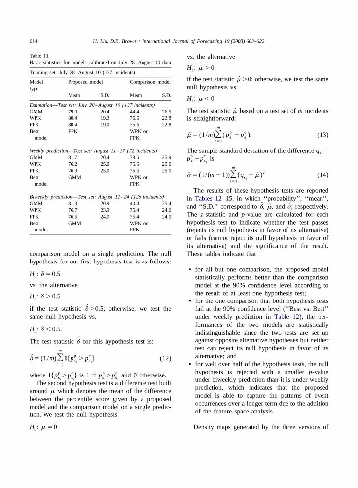
T able 11 vs. the alternativeBasic statistics for models calibrated on July 28–August 10 data

H : m .0aTraining set: July 28–August 10 (137 incidents)îf the test statisticm.0; otherwise, we test the sameModel Proposed model Comparison model

null hypothesis vs.typeMean S.D. Mean S.D.

H : m ,0.aEstimation—Test set: July 28–August 10 (137 incidents)

ˆThe test statisticm based on a test set ofm incidentsGMM 79.0 20.4 44.4 26.5WPK 80.4 19.3 75.6 22.8 is straightforward:FPK 80.4 19.0 75.6 22.8 mBest FPK WPK or p c

m̂ 5 (1 /m)O( p 2 p ). (13)s smodel FPK i ii51

Weekly prediction—Test set: August 11–17 (72 incidents) The sample standard deviation of the differenceq 5s ip cGMM 81.7 20.4 38.5 25.9 p 2p iss si iWPK 76.2 25.0 75.5 25.0m

FPK 76.0 25.0 75.5 25.0 2ˆ ˆs5 (1 /(m 21))O(q 2m ) (14)sBest GMM WPK or ii51

model FPKThe results of these hypothesis tests are reported

Biweekly prediction—Test set: August 11–24 (126 incidents) in Tables 12–15,in which ‘‘probability’’, ‘‘mean’’,GMM 81.0 20.9 40.4 25.4 ˆ ˆ ând ‘‘S.D.’’ correspond tod, m, ands, respectively.WPK 76.7 23.9 75.4 24.0

The z-statistic andp-value are calculated for eachFPK 76.5 24.0 75.4 24.0hypothesis test to indicate whether the test passesBest GMM WPK or

model FPK (rejects its null hypothesis in favor of its alternative)or fails (cannot reject its null hypothesis in favor ofits alternative) and the significance of the result.

comparison model on a single prediction. The null These tables indicate thathypothesis for our first hypothesis test is as follows:

• for all but one comparison, the proposed modelH : d 50.50 statistically performs better than the comparisonvs. the alternative model at the 90% confidence level according to

the result of at least one hypothesis test;H : d .0.5a • for the one comparison that both hypothesis testsîf the test statisticd.0.5; otherwise, we test the fail at the 90% confidence level (‘‘Best vs. Best’’

same null hypothesis vs. under weekly prediction inTable 12), the per-formances of the two models are statistically

H : d ,0.5.a indistinguishable since the two tests are set upˆ against opposite alternative hypotheses but neitherThe test statisticd for this hypothesis test is:

test can reject its null hypothesis in favor of itsmp c alternative; andd̂ 5 (1 /m)O1hp . p j (12)s si i

i51 • for well over half of the hypothesis tests, the nullhypothesis is rejected with a smallerp-valuep c p cwhere1hp .p j is 1 if p .p and 0 otherwise.s s s si i i i under biweekly prediction than it is under weeklyThe second hypothesis test is a difference test builtprediction, which indicates that the proposedaroundm which denotes the mean of the differencemodel is able to capture the patterns of eventbetween the percentile score given by a proposedoccurrences over a longer term due to the additionmodel and the comparison model on a single predic-of the feature space analysis.tion. We test the null hypothesis

H : m 5 0 Density maps generated by the three versions of0


T able 12Hypothesis tests results for models calibrated on July 7–20 data

Training set: July 7–20 (145 incidents)

Comparison Test 1 Test 2

Probability z-Statistic p-Value Mean S.D. z-Statistic p-Value

Estimation—Test set: July 7–20 (145 incidents)GMM vs. GMM 0.883 9.22 ,0.001 27.7 26.3 12.71 ,0.001WPK vs. WPK 0.938 10.55 ,0.001 6.5 7.9 9.87 ,0.001FPK vs. FPK 0.910 9.88 ,0.001 6.5 8.1 9.69 ,0.001Best vs. Best 0.910 9.88 ,0.001 6.5 8.1 9.69 ,0.001

Weekly prediction—Test set: July 21–27 (72 incidents)GMM vs. GMM 0.750 4.24 ,0.001 19.8 32.5 5.17 ,0.001WPK vs. WPK 0.583 1.41 0.079 2.0 11.0 1.53 0.063FPK vs. FPK 0.597 1.65 0.050 1.8 11.0 1.43 0.076Best vs. Best 0.444 0.94 0.174 2.3 19.4 1.02 0.154

Biweekly prediction—Test set: July 21–August 3 (140 incidents)GMM vs. GMM 0.729 5.41 ,0.001 18.9 31.2 7.15 ,0.001WPK vs. WPK 0.586 2.03 0.021 1.86 7.8 2.80 0.003FPK vs. FPK 0.586 2.03 0.021 1.64 8.0 2.42 0.008Best vs. Best 0.479 0.51 0.305 3.32 15.8 2.49 0.006

the proposed model built on the training data set of within the immediate following week and 2 weeksthe 145 incidents between July 7 and July 20 are (i.e., the test sets for weekly and biweekly predictiongiven in Fig. 3. The criminal incidents occurring scenarios) are plotted on the density maps to enable

T able 13Hypothesis tests results for models calibrated on July 14–27 data

Training set: July 14–27 (143 incidents)



Estimation—Test set: July 14–27 (143 incidents)GMM vs. GMM 0.783 6.77 ,0.001 19.5 28.00 8.31 ,0.001WPK vs. WPK 0.902 9.62 ,0.001 5.9 7.54 9.33 ,0.001FPK vs. FPK 0.902 9.62 ,0.001 5.9 7.70 9.23 ,0.001Best vs. Best 0.902 9.62 ,0.001 5.9 7.70 9.23 ,0.001

Weekly prediction—Test set: July 28–August 3 (68 incidents)GMM vs. GMM 0.809 5.09 ,0.001 17.06 27.71 5.08 ,0.001WPK vs. WPK 0.603 1.70 0.045 2.47 8.35 2.44 0.007FPK vs. FPK 0.588 1.46 0.072 2.16 8.51 2.09 0.018Best vs. Best 0.544 0.73 0.233 6.17 14.78 3.44 ,0.001

Biweekly prediction—Test set: July 28–August 10 (137 incidents)GMM vs. GMM 0.766 6.24 ,0.001 16.07 29.57 6.36 ,0.001WPK vs. WPK 0.620 2.82 0.002 2.25 8.70 3.02 0.001FPK vs. FPK 0.577 1.79 0.037 2.06 8.80 2.74 0.003Best vs. Best 0.518 0.43 0.334 3.83 16.74 2.68 0.004


T able 14Hypothesis tests results for models calibrated on July 21–August 3 data

Training set: July 21–August 3 (140 incidents)



Estimation—Test set: July 21–August 3 (140 incidents)GMM vs. GMM 0.829 7.78 ,0.001 19.6 27.1 8.59 ,0.001WPK vs. WPK 0.857 8.45 ,0.001 3.6 5.5 7.75 ,0.001FPK vs. FPK 0.857 8.45 ,0.001 3.57 5.8 7.24 ,0.001Best vs. Best 0.857 8.45 ,0.001 3.6 5.5 7.75 ,0.001

Weekly prediction—Test set: August 4–10 (69 incidents)GMM vs. GMM 0.797 4.94 ,0.001 19.0 29.9 5.28 ,0.001WPK vs. WPK 0.565 1.08 0.140 2.1 10.8 1.60 0.055FPK vs. FPK 0.580 1.32 0.093 2.0 11.00 1.53 0.063Best vs. Best 0.580 1.32 0.093 6.1 19.2 2.62 0.004

Biweekly prediction—Test set: August 4–17 (141 incidents)GMM vs. GMM 0.830 7.83 ,0.001 21.4 28.0 9.08 ,0.001WPK vs. WPK 0.532 0.76 0.224 1.1 4.9 2.60 0.005FPK vs. FPK 0.553 1.26 0.104 0.9 5.0 2.15 0.016Best vs. Best 0.560 1.43 0.076 5.5 16.9 3.83 ,0.001

visual examination of how well the proposed model maps that most of the incidents in the test sets indeedperforms under weekly and biweekly prediction occurred around the predicted high-density areas.scenarios, respectively. It is easily seen on these Also by visual inspection, the GMM version of the

T able 15Hypothesis tests results for models calibrated on July 28–August 10 data

Training set: July 28–August 10 (137 incidents)



Estimation—Test set: July 28–August 10 (137 incidents)GMM vs. GMM 0.839 7.95 ,0.001 34.6 38.6 10.49 ,0.001WPK vs. WPK 0.891 9.145 ,0.001 4.9 8.4 6.79 ,0.001FPK vs. FPK 0.832 7.78 ,0.001 4.9 8.6 6.61 ,0.001Best vs. Best 0.832 7.78 ,0.001 4.9 8.6 6.61 ,0.001

Weekly prediction—Test set: August 11–17 (72 incidents)GMM vs. GMM 0.889 6.60 ,0.001 43.1 36.0 10.17 ,0.001WPK vs. WPK 0.597 1.65 0.050 0.8 6.0 1.08 0.140FPK vs. FPK 0.611 1.89 0.029 0.5 6.0 0.73 0.233Best vs. Best 0.528 0.47 0.319 6.2 18.0 2.92 0.002

Biweekly prediction—Test set: August 11–24 (126 incidents)GMM vs. GMM 0.897 8.91 ,0.001 40.5 37.0 12.26 ,0.001WPK vs. WPK 0.611 2.49 0.006 1.4 9.8 1.56 0.059FPK vs. FPK 0.611 2.49 0.006 1.1 9.8 1.29 0.099Best vs. Best 0.524 0.54 0.298 5.5 18.8 3.31 0.001


Fig. 3. GMM (upper), WPK (middle), and FPK (lower) versions of the proposed model calibrated on July 7–20 data and tested on July21–27 data (left) and July 21–August 3 data (right).


proposed model captured more spatial variation than A.1. Partition event feature dataeither the WPK or FPK versions. This explains theresults inTables 8–11where the GMM version is Intuitively, the numberC of the clusters in the keypicked as the best model for every weekly or feature space corresponds to the number of distinctbiweekly prediction scenario. sets of criminal preferences. Unless we have clusters

a priori (e.g., crime analysts may tell us how manygroups of offenders are likely to be represented bythe data), we have to ‘‘discover’’ it from the data.5 . ConclusionTechnically, the purpose of partitioning feature datais to accommodate local covariance structures in theIn this paper, we have described a newly de-component density models that we will examineveloped space–time prediction model for crimemomentarily. To accomplish this first task, we use apoints and evaluated it on breaking and enteringhierarchical clustering algorithm to generate parti-burglary point data from Richmond, VA. The pro-tions and employ a stopping rule to determine whichposed model is shown to be more effective than thepartition is the best.best of current ‘‘hot spot’’ methods. Some important

For a data set of sizen, a hierarchical clusteringcharacteristics of this approach include:algorithm generates a succession ofn partitionsP ,0

P , . . . , P , where P , P , . . . , P contain n,1 n21 0 1 n21• inclusion of measurable features that are usefuln21, . . . , 1 cluster(s), respectively. It merges twofor prediction;‘‘closest’’ clusters inP to generateP at each step.j j11• identification of the features with the most predic-What we mean by ‘‘closest’’ obviously depends ontive or explanatory power; andthe definition of cluster-to-cluster distance. This• presentation of forecasts through probability den-definition distinguishes different variants of thesity estimates over space and time.algorithm. We will not delve into the details and theinterested reader is referred toEveritt (1991)for an

Our prediction modeling can be integrated into anintroduction. The stopping rule that we use is a

interactive shared information and decision supportrevision of Mojena (1977).Let a be the shortestjsystem such as ReCAP(Brown, 1998)to aid crimedistance between any two clusters in the partitionPjfighting in an automated fashion.( j50, 1, . . . , n21). Then revised rule is to stopmerging clusters further and select the first partitionP satisfyingj

A cknowledgements¯a .a 1 k ? s (A.1)j11 j aj

This project was partially supported by grant no.¯NIJ 98-LB-VX008 awarded by the National Institute wherea ands are the mean and unbiased standardj aj

of Justice, Office of Justice Programs, U.S. Depart- deviation of a , a , . . . , a , and the constantk is0 1 j

ment of Justice. Points of view in this document are usually set to 1.25, as recommended byMilligan andthose of the author and do not necessarily representCooper (1985).When n is large, we find that thisthe official position or policies of the U.S. Depart- revised rule yields similar result toMojena (1977).ment of Justice. The rationale of these rules is to look for significant

‘‘jump’’ in the a series.

A.2. Estimate first-order spatial transition densityA ppendix A. Model component estimation and spatial interaction probabilities

We consider two classes of models for estimatingThis section addresses the four tasks listed inthe first-order spatial transition density. Both classesSection 3 for estimating individual components ofplay roles in modeling data from multiple underlyingour transition density model.


categories and sources. The first class is calledfinite parametric techniques and was introduced byMar-mixture distributions (e.g., Everitt & Hand, 1981; chette, Priebe, Rogers, and Solka (1996).They areMcLachlan & Basford, 1988; Titterington, Smith, & collectively calledfiltered kernel estimators (FKE)Makov, 1985). These distributions are superpositions and take the formof component distributions. A finite mixture prob-ability density function (or mass function in the case n C r (x )1 j i 21ôf discrete sample space) has the form ] ]]f(x)5 OO K(H (x2 x )) (A.3)j in uH ui51j51 j

C

f(x;p,Q)5Op f (x;u ) (A.2)j j j where K(?) is called akernel function, H , j5 1,j51 j

2, . . . , C, are C p3p nonsingularlocal bandwidthwherep .0, j51, 2, . . . ,C, p 1p 1???1p 51, matrices and r (x), j51, 2, . . . ,C, which satisfyj 1 2 C jp5[p ???p ]9, Q5[u ? ? ?u ]. f (x; u ) is the jth1 C 1 C j j

component density with the setu of parameters andj C

p , p , . . . , p are mixing weights. Q is the collec-1 2 C 0#r (x)# 1 andOr (x)5 1 (A.4)j jtion of all component parameters. To fit a finite j51

mixture distribution, one needs to find the numberCof component densities first. In our case this was for all x, are filtering functions. Local bandwidthdone in the previous subsection—partitioning event matrices contain posterior parameter settings thatfeature datahx : i51, 2, . . . ,nj.i enforce localized smoothness. The filtering functions

Two aspects need to be addressed further in orderare prior weights over variations of local smooth-for us to generate a density estimate by Eq. (A.2). ness. We only consider a special case of Eq. (A.3) forFirst, further assumptions need to be made on the our purpose where we setH 5diag[h ? ? ?h ], j51,j j1 jpfunctional form of the component densitiesf (x; u )j j 2, . . . ,C, whereh ( j51, 2, . . . ,C; l51, 2, . . . , p)jl( j51, 2, . . . , C). For a continuous feature space is a local bandwidth for thelth dimension [x] of thel(where all features are continuous variables) we use jth locally varied region of support. We call theseGaussian mixture models (GMM), wheref (x; u ),j j special class of estimatorsfiltered product kernelj51, 2, . . . ,C, are postulated as multivariate Gaus- (FPK) estimators. The underlying assumption forsian. In the discrete case, we fit the data with a class FPK estimators is that all dimensions are mutuallyof Latent Class Models (LCM) (seeEveritt, 1984), independent.where we assume that the categorical feature vari- In this paper we assume that the kernel function isables are independent and the outcomes of eachthe standard multivariate Gaussian density function.variable are also independent. For the situation To generate a density estimate by Eq. (A.3), we needwhere mixed variable types are present, it is trivial to to specify the filtering functions as well as the localcombine GMM and LCM provided that the numeric bandwidths. Suppose the datahx : i51, 2, . . . , njidimensions are independent of the categorical ones.have been partitioned intoC clustersV , V , . . . ,1 2Second, we need an algorithm to estimate the V . We derive the filtering functions in one of theCparametersp5[p ???p ]9 and Q5[u ? ? ?u ]. We1 C 1 C following two ways:use a numeric maximum likelihood algorithm knownas Expectation-Maximization (EM) algorithm (see,

C• Fit a finite mixture modelg(x)5o p g (x) tofor example,Dempster, Laird, & Rubin, 1977). This j51 j j

the data. Setalgorithm first calculates these parameters with re-spect to the clusters in the feature space partition,and then updates them iteratively until the log r (x)5p g (x) /g(x), j 51,2,. . . ,C (A.5)j j j

nlikelihood L 5o log f(x ;p,Q) converges to ai51 i

stationary point.The second class of models we use to estimate the • Let the indicator1 be 1 if x[V and 0hx[V j j

first-order spatial transition density belongs to non- otherwise. Set


r (x)5 1 , j 5 1,2,. . . ,C (A.6) A.3. Estimate second-order spatial transitionj hx[V jjdensities

We term the FPK estimators with the filtering The third task is to estimate second-order spatialfunctions defined by Eq. (A.6)weighted product transition densities. The models we choose for thesekernel ( WPK) estimators. Let n be the number ofj densities maintain continuity in parallel with thedata points in clusterV . The local bandwidths arej ordering of inter-event geographic distances and/orestimated by using local data in each cluster. To wit, that of inter-event temporal distances. Such orderings

reflect additional assumptions on site selection be-1 / ( p14)4 havior. First, given that two geographic locations21 / ( p14)ˆ ]] ˆh 5 s n ,S Djl jl j have the same set of feature values, it is reasonablep 1 2

to postulate thatevent initiators are in favor of thel 5 1,2,. . . ,p, j 5 1,2,. . . ,C (A.7)

geographically closer location to start the next event.This assumption is supported by the ‘‘journey to

ˆwheres is the standard deviation of thelth variable crime’’ theory in criminology. In view of thisjl

[x] estimated from the unidimensional local data set assumption, a model of spatial interaction shouldl

h[x ] : x [V j. Notice that these bandwidth estimates give decreasing weight to past events with increasingi l i j

are optimal in the Approximate Mean Integrated distance to the location of interest. Another be-Square Error (AMISE) sense when they are used to havioral assumption that may hold true for certainfit Gaussian product kernel estimators to the local scenarios (e.g., serial crimes of certain type) is thatdata setshx [V j, j51, 2, . . . ,C, which are in fact event initiators tend not to wait long before they acti j

samples of multivariate Gaussian distributions (see again. A model incorporating this assumption shouldScott, 1992). weigh the impacts of past events on future events

When we use either finite mixture or filtered according to their ‘‘ages’’. The more recently ankernel estimators to model first-order spatial transi- event occurred, the higher weight it gets. Twotion density, models of distinct local structures are models developed byFiksel (1984),known as thesimultaneously specified. Spatial interaction prob- order model and the instant model, both incorporateabilities are estimated using these ‘‘local’’ models. the journey to event assumption, while the instantWhen a finite mixture distribution is involved, spatial model also takes into account the assumption regard-interaction probabilities are given as ing the lingering period to resume act. We describe

these models below.( j ) ( j ) Let the number of data units in clusterj be m. LetPrhx [ x ux j5p f (x ;u ) /f(x ;p,Q),n11 n j j n11 j n11

( j ) ( j )D 5hs , s , . . . , s j and T 5ht , t , . . . , t jn 1 2 m n 1 2 mj 5 1,2,. . . ,C (A.8) where t ,t , . . . ,t and s , s , . . . , s are or-1 2 m 1 2 m

dered according tot , t , . . . , t . Adapting Fiksel’s1 2 m

When a filtered kernel estimator is used, spatial order model to our case, we postulate the followinginteraction probabilities are given as function for the second-order spatial transition den-

sity for clusterj( j ) ( j ) ˆ ˆPr(x [ x ux )5 f (x ) / f(x ),n11 n j n11 n11

12 ( j ) ( j )c (suD ,T ,t)5w (sus , . . . ,s )j 5 1,2,. . . ,C (A.9) n n n m 1 m

2 ml 2lis2s ii]]5 Oe (A.11)where 2pm i51

n r (x )1 j i 21ˆ ] ]]f (x )5 O K(H (x 2 x )), where t.t is a future event’s time of occurrencej n11 j n11 i mn uH ui51 j and is2s i the distance from that future event’si

j 5 1,2,. . . ,C (A.10) location s to an older event locations (i51, 2, . . . ,i


B rown, D. E. (1998). The Regional Crime Analysis Programm). This is called an order model since only the(ReCAP): A framework for mining data to catch criminals.temporal order of the events is considered. TheProceedings of 1998 IEEE International Conference on Sys-

instant model actually utilizes the values of the series tems, Man, and Cybernetics, 2848–2853.t , t , . . . , t . Based on this model, we postulate that C apone, D., & Nichols, W. (1976). Urban structure and criminal1 2 m

the second-order spatial transition density for cluster mobility. American Behavioral Scientist, 20, 199–213.C ensusCD1maps, Version 2.0 (1998). GeoLytics, East Brun-j takes on the form

swick, NJ.C ressie, N. A. C. (1993).Statistics for spatial data. New York:

12 ( j ) ( j ) Wiley.c (suD ,T ,t)5h (sus , . . . ,s , t , . . . ,t ,t)n n n m 1 m 1 mD empster, A. P., Laird, N. M., & Rubin, D. B. (1977). Maximum

2 m likelihood estimation from incomplete data via the EM algo-l 2lis2s i2t (t2t )i i]]]]5 Oem rithm (with discussion). Journal of the Royal Statisticali512t (t2t )i Society. Series B, 39, 1–38.2pOe

D iggle, P. J. (1983).The statistical analysis of spatial pointi51

patterns. London: Academic Press.(A.12) E veritt, B. S. (1984).An introduction to latent variable models.

London: Chapman & Hall.E veritt, B. S. (1991).Cluster analysis. 3rd ed.. London: EdwardFor both Eqs. (A.11) and (A.12), we can numerically

Arnold.solve for the maximum likelihood estimates of theE veritt, B. S., & Hand, D. J. (1981).Finite mixture distributions.

parameters (i.e.,l in Eq. (A.11), l and t in Eq. London: Chapman & Hall.(A.12)). The interested reader is referred toFiksel F iksel, T. (1984). Simple spatial–temporal models for sequences

of geological events.Elektronische Informationsverarbeitung(1984).und Kybernetik, 20, 480–487.

J efferis, E. (1998). A multi-method exploration of crime hot spots.Presentation at the Annual Meeting of the Academy of A.4. Estimate geographic-space feature densityCriminal Justice Sciences, Albuquerque, NM, March 10–14,1998.

The fourth and last task is to estimate the geog- L eBeau, J. L. (1987). The journey to rape: Geographic distanceand the rapist’s methods of approaching the victim.Journal ofraphic-space feature density when appropriate andPolice Science and Administration, 15, 129–136.possible. In general, this requires sampling over the

L evine, N. (1998). ‘‘Hot Spot’’ analysis usingCrimeStat kernelstudy region. For example, we obtain feature valuesdensity interpolation.Presentation at the Annual Meeting of

for sample locations chosen uniformly and indepen- the Academy of Criminal Justice Sciences, Albuquerque, NM,dently over the study region. We then fit a density March 10–14, 1998.function to these sample values using either finite M archette, D. J., Priebe, C. E., Rogers, G. W., & Solka, J. L.

(1996). Filtered kernel density estimation.Computationalmixture or filtered kernel method.Statistics, 11, 95–112.

M cLachlan, G. J., & Basford, K. E. (1988).Mixture models:Inference and applications to clustering. New York: MarcelDekker.

R eferences M illigan, G. W., & Cooper, M. C. (1985). An examination ofprocedures for determining the number of clusters in a data set.Psychometrika, 50, 159–179.A mir, M. (1971).Patterns in forcible rape. Chicago: University of

M ojena, R. (1977). Hierarchical grouping methods and stoppingChicago Press.rules: An evaluation.Computer Journal, 20, 359–363.B aldwin, J., & Bottoms, A. (1976).The urban criminal: A study

M olumby, T. (1976). Patterns of crime in a university housingin Sheffield. London: Tavistock Publications.project. American Behavioral Scientist, 20, 247–259.B lock, C. (1995). STAC hot-spot areas: A statistical tool for law

N ewman, O. (1972).Defensible space: Crime prevention throughenforcement decisions. In Block, C. R., Dabdoub, M., &urban design. New York: Macmillan.Fregly, S. (Eds.),Crime analysis through computer mapping.

R epetto, T. A. (1974).Residential crime. Cambridge, MA:Washington, DC: Police Executive Research Forum, p. 20036.Ballinger.B rantingham, P., & Brantingham, P. (1975). Spatial patterns of

R ossmo, D. K. (1993). Target patterns of serial murders: Aburglary.Howard Journal of Penology and Crime Prevention,methodological model.American Journal of Criminal Justice,14, 11–24.17(2), 1–21.B rantingham, P., & Brantingham, P. (1984).Patterns in crime.

New York: Macmillan Publishing.


R ossmo, D. K. (1996). Targeting victims: Serial killers and the He has conducted research in the areas of inductive modeling,urban environment. In O’Reilly-Flemming, T. (Ed.),Serial and intelligent systems, probabilistic models, and discrete-event simu-mass murder: Theory, research, and policy. Toronto: Canadian lation. He holds a BS degree from Tianjin University, China, andScholars Press. MS and PhD degrees from University of Virginia, all in Systems

Engineering.S carr, H. A. (1973).Patterns in burglary. 2nd ed.. Washington,DC: U.S. Department of Justice.

S cott, D. W. (1992).Multivariate density estimation. New York: Dr. Donald E. BROWN is Professor and Chair of the DepartmentWiley. of Systems and Information Engineering at University of Virginia.

T itterington, D. M., Smith, A. F. M., & Makov, U. E. (1985). He is also Director of the Critical Incident Data Analysis CenterStatistical analysis of finite mixture distributions. New York: and Editor of the IEEE Transactions on Systems, Man, andWiley. Cybernetics, Part A. He is a fellow of the IEEE and the 2002

winner of the Norbert Wiener Award from the IEEE Systems,Man, and Cybernetics Society for outstanding contributions toBiographies: Dr. Hua LIU works as a Senior Software Engineerresearch and education in systems engineering. He is a recipient ofwith CSG Systems, a leading provider of billing and customerthe Millennium Medal from the IEEE. He received his PhD fromcare software. Prior to CSG, he was a Member of Technical StaffUniversity of Michigan, the MS and ME degrees from thewith Lucent Technologies. His industrial experience includesUniversity of California, Berkley, and the BS degree from theresearch and development of state-of-the-art communication soft-U.S. Military Academy, West Point.ware, and large-scale systems modeling, control and optimization.

Date post:	24-Jun-2018
Category:	Documents
Upload:	nguyendieu
View:	219 times
Download:	0 times

C riminal incident prediction using a point-pattern … riminal incident prediction using a...

Documents