126
© C. Ronniger 2012 1 © 2012 Curt Ronniger
| Date post: | 08-Mar-2018 |
| Category: |
Documents |
| Upload: | phamnguyet |
| View: | 214 times |
| Download: | 2 times |

© C. Ronniger 2012 1
© 2012 Curt Ronniger

2 © C. Ronniger 2012

© C. Ronniger 2012 3
Content 1. Test methods ........................................................................................................ 7
Components Search .................................................................................................... 8
Scatter Plot (Realistic Tolerance Parallelogram(SM) Plot) ........................................... 9
Measurement-Comparison (Isoplot (SM) ) .................................................................... 10
Multi-Vari-Chart(SM) ..................................................................................................... 11
Paired Comparison .................................................................................................... 12
Comparison B vs. C(SM) ........................................................................................... 13
Intensity-Relation-Matrix ............................................................................................ 15
Priority Matrix ............................................................................................................. 16
Matrix diagram ........................................................................................................... 18
2. Analysis of Variance (ANOVA) .......................................................................... 19
Basics ........................................................................................................................ 19
SS = Sum of Squares................................................................................................ 19
ANOVA between two Series ...................................................................................... 20
ANOVA & ANOM with several Factors ....................................................................... 22
3. Design of Experiment ......................................................................................... 26
Design ........................................................................................................................ 26
Full-, fractional and Taguchi experiments .................................................................. 27
Plackett-Burman-experiments .................................................................................... 29
Orthogonality .............................................................................................................. 30
Taguchi ...................................................................................................................... 30
Full-factorial quadratic ................................................................................................ 31
Central Composite Design ......................................................................................... 31
Box-Behnken design .................................................................................................. 32
D-Optimal experiments .............................................................................................. 33
Mixture experiments ................................................................................................... 34
Correlation ................................................................................................................. 38
4. Regression .......................................................................................................... 40
General ...................................................................................................................... 40
Linear Regression ...................................................................................................... 40
Linear regression through 0-point .............................................................................. 41
Nonlinear regression .................................................................................................. 42
Regression types ....................................................................................................... 42
Multiple Regression .................................................................................................... 45
Analyses of Variance (Model ANOVA) ....................................................................... 49
Prediction Measure Q² ............................................................................................ 50
Lack of Fit ............................................................................................................... 51
Analyses of Variance overview ............................................................................... 51
Reproducibility ........................................................................................................ 52
Test of the coefficient of determination ................................................................... 52
Test of the regression coefficients, the p-value ...................................................... 52
Test of the coefficient of determination ................................................................... 53
Standard deviation of the model RMS .................................................................... 54
Confidence interval for the regression coefficient ................................................... 54
Confidence interval for the response ...................................................................... 54
Condition Number ................................................................................................... 54
Standardize to -1 ... +1 ........................................................................................... 55
Standardize to standard deviation .......................................................................... 55
The correlation matrix ............................................................................................. 55

4 © C. Ronniger 2012
Response transformation (Box-Cox) .......................................................................... 56
Statistical charts for multiple regression ..................................................................... 58
Regulation of outliers .............................................................................................. 61
Optimization............................................................................................................ 62
If certain response values have maybe a higher importance than other, this can be taken into account by a weighting factor δ. ............................................................. 63
Discrete Regression ................................................................................................... 64
Discrete regression bases .......................................................................................... 64
5. Multivariate Analises .......................................................................................... 70
Cluster Analysis ......................................................................................................... 70
Principal Component Analysis PCA ........................................................................... 74
Partial Least Square (PLS) ........................................................................................ 76
Estimation of the spread at PLS ............................................................................. 77
Variable selection with VIP ..................................................................................... 78
6. Neural Networks ................................................................................................. 80
Topology .................................................................................................................... 80
Training-Algorithm ...................................................................................................... 82
Neural Network as an alternative for multiple regression ........................................... 83
Attributes of Neural Networks .................................................................................... 84
Example ..................................................................................................................... 85
Further statistical charts ........................................................................................ 86
Scatter bars ................................................................................................................ 86
Boxplot ....................................................................................................................... 87
Median plot ................................................................................................................ 88
Gliding average .......................................................................................................... 88
Pareto ........................................................................................................................ 90
7. Capability indices ............................................................................................... 91
In following the relations are shown for different distribution forms: ........................... 91
Normal distribution ..................................................................................................... 91
Lognormal-distribution ................................................................................................ 92
Folded normal distribution 1st type ............................................................................ 92
Folded normal distribution 2nd type (Rayleigh-distribution) ....................................... 93
Non-parametric (distribution free) Percentil-method ................................................... 93
Distributions forms for several design characteristics ................................................ 94
Applications for capability studies: ............................................................................. 94
Measurement System Analysis .................................................................................. 95
Type-1 Study .......................................................................................................... 95
Type-2 Study .......................................................................................................... 95
Type-3 Study .......................................................................................................... 96
MSA Gage R&R ..................................................................................................... 96
Measurement System Analysis with ANOVA.......................................................... 98
8. Statistical Tests and Evaluations ...................................................................... 99
χ²-Test of goodness of fit ........................................................................................... 99
χ²-Homogeneity test ................................................................................................. 100
χ²- Multi field test ...................................................................................................... 101
Binomial-test ............................................................................................................ 102
Kolmogorov-Smirnov-Assimilation test ..................................................................... 103
Shapiro-Wilk test ...................................................................................................... 103
Anderson-Darling test of normal-distribution ............................................................ 104
t-test for two samples ............................................................................................... 105
Test for comparison of one sample with a default value .......................................... 106
U-test for two samples ............................................................................................. 107

© C. Ronniger 2012 5
F-test ........................................................................................................................ 108
Outlier test ................................................................................................................ 108
Balanced simple Analysis of Variance ..................................................................... 110
Bartlett-test ............................................................................................................... 111
Rank dispersion test according to Siegel and Tukey ................................................ 112
Test of an best fit straight line .................................................................................. 113
Test on equal regression coefficients ....................................................................... 113
Linearity test ............................................................................................................. 113
Gradient test of a regression .................................................................................... 114
Independence test of p series of measurements ..................................................... 114
9. Normal-distribution .......................................................................................... 115
Divergences of the normal distribution ..................................................................... 117
10. Statistical factors ............................................................................................ 118
11. Literature ......................................................................................................... 119
12. Index ................................................................................................................ 127

6 © C. Ronniger 2012
1. Software
For the methods and procedures which are shown here the software Visual-XSel®
12.0
is used.
For the first steps use the icons on the start picture and follow the menus and hints. There are also templates with examples (like methods after Shainin). For this use the menu Templates -> Shainin… The CRGRAPH-software can be downloaded via www.crgraph.com/XSel12eInst.exe

© C. Ronniger 2012 7
1. Test methods Under test methods there are statistical methods to understand which were developed through Shainin /1/ and Taguchi /3/. These are also known under the system optimiza-tion. The goal is to find the most important influences in technical or other processes, with a minimum of parts and tests. The products and their productional processes can be improved decisively with these mostly very simple methods. In the following descriptions there are no derivations of the formulas. The priority is much more the application for the practice. On further-reaching information the literature is therefore referred. To every method there are file templates to comprehend this one with easily examples of Visual-XSel®. The files marked in italics in the overviews and descriptions in blue represent these presentations. The procedure is always the same: Put your data into the table (marked often with yellow background) and start the program with F9. The re-sults are shown then in the main window. The following issues are treated:
• Test methodes from Shainin and others
• Taguchi strategy and experiments
• Standard experiments and D-optimal
• Variance - analysis
• Statistical diagrams and spezial charts
• Correlation and regression
• Multiple Regression (stepwise regression)
• Multivariate analyses
• Statistical tests and evaluations
• Statistical distributions
• Optimization Templates for standard statistics and hypothesis test are provide in the subdirectory \Statistics Templates for Shainin and examples are provided in the subdirectory \StatisticalMethods Experiments and there evaluation with Multiple Regression or Neural Networks are available via the Data Analysis Guide Hint: Shainin
® and Red-X
® and Visual-XSel ® are Trademarks.

8 © C. Ronniger 2012
Components Search With the component test e.g. an error cause at a ”device” should be found. For this a device with a defective performance is necessary and one, which shows faultless cha-racteristics. Precondition for this method is that the devices can be disassembled non-destructively. Here the performance should not be changed considerably by the re-assembly. Before, it has to be fixed, which components resp. single modules have to be exchanged. The process can be multilevel, that means if a subassembly is found as the relevant one, this also can be demounted into its devices. So that the number of mountings is as small as possible, preferably big units should be used in the beginning. To differentiate a substantially change compared to the not precluded straggling, first the devices must be disassembled in the beginning and reassembled (repeat trials). This should take place at least twice. From the first measuring and the repetitions after the disassembly a scatter band results (d1 and d2).
The proportion of the medium discrepancies (D) of the corresponding measurements to those within a device is not permitted to fall below the factor 5. Now successively the exchange of the devices starts. There the devices with the proba-bly major influence should be exchanged first. After each mounting the devices have to be reconstructed, whatever there was a variation or not. Just then the next device should be exchanged. At the test overview the results of the good and of the worse devices are pictured as line chart and the particular changes are valuated in the distribution. In the validation trial all devices, which have changed the result, are exchanged together and the result is also en-tered.
D
d1
d2
Rs1
Rs2
Rg1
Rg2
Sta
rt
Wie
der-
holu
ng
2
21
2
21 RgRgRsRsD
+−
+=
2
21
2
21 RgRgRsRsd
−+
−=
D : d ≥ 5
Start Repetition
Sta
rt t
es
t
Re
pe
tito
n 1
Re
pe
titi
on
2
Co
mp
. A
Co
mp
. B
Co
mp
. C
Co
mp
. D
Co
mp
. E
Co
mp
. F
Co
nfi
rma
tio
n 1
Co
nfi
rma
tio
n 2
Qu
ality
ch
ara
cte
risti
c
0
2
4
6
8
10
12
Sta
rt t
es
t
Re
pe
tito
n 1
Re
pe
titi
on
2
Co
mp
. A
Co
mp
. B
Co
mp
. C
Co
mp
. D
Co
mp
. E
Co
mp
. F
Co
nfi
rma
tio
n 1
Co
nfi
rma
tio
n 2
0
2
4
6
8
10
121212
111111.511.5
1212
1111
1313
33
44
22
44
33
44
1010
99
66
88
3.53.5 3.43.4 3.63.6
11.511.511.211.2 11.411.4

© C. Ronniger 2012 9
If the measured data alter in the middle, outside the scatter band, so more or less big influences are transparent, which depict a reciprocation (here comp. A and D). If the measured data are cross-over in the respectively other scatter zone, so the device resp. component with the critical influence is found.(the so called red X). This method can be executed with help of the template file Components_Search.vxg .
Scatter Plot (Realistic Tolerance Parallelogram(SM) Plot) In the classical linear regression an optimal best fit straight line is set through the meas-ured values. In dependency of the straggling of the breakpoints those are more or less far away from this straight line. If a distribution is generated for these deviations (resi-dues), you can determine a frequency region for the number of points. As a rule the 95%-region is depicted, that means 95% of all breakpoints are in the hatched depicted parallel band around the straight line. Precondition for these considerations is of course the normal distribution of the measured values.
If there are requests for the target value, those can be entered (green horizontal lines) and be drawn to the respectively upper and lower frequency region. The perpendicular lines show the tolerance range on the x-axis necessary for this. This of course is nar-rower than the one, as if just the best fit straight line would be used, because the scatter band has to be taken into consideration. This method can be executed with help of the template file Scatter_Plot.vxg. Optional the target value region requested here can be default. After start of the program the up-per and lower tolerance range and the corresponding median are issued. If the indica-tion of the target value is open, automatically the smallest and biggest measured value is used.
Tolerance
1.0 1.5 2.0 2.5 3.0
Fu
nc
tio
na
l re
sp
on
se
0
1
2
3
4
5
6
1.0 1.5 2.0 2.5 3.0
0
1
2
3
4
5
6

10 © C. Ronniger 2012
Measurement-Comparison (Isoplot (SM) )
The display format of the measurement equipment capability is very similar to the Scat-ter-Plot. But here it is a matter of comparison of two measuring methods. The results of one measurement is spread over the other. The linear regression is below a 45° line (same measure for X and Y). If a distribution for those variances of measured values (residues) is built, you can determine a frequency region for the number of points. Nor-mally the 95%-region is depicted, that means 95% of all breakpoints are in the hatched depicted parallel band around the straight line. Precondition for those considerations is that the measured values are normal distributed. At least 30 measured values should be available.
∆P is determined from both factors L and ∆Μ:
22
22ML
P∆
−=∆
The so called resolving power should be
6≥∆
∆
M
P
If the best fit straight line is parallel shifted to the 45°-line, there is a constant deviation. If it generates a striking other angle than 45°, this is a variable deviation. This method can be executed with help of the template file Isoplot.vxg.
(SM) Isoplot is a Service Mark of Shainin corp.
Data 1
0.1 0.2 0.3 0.4 0.5 0.6 0.7
Da
ta 2
0.1
0.2
0.3
0.4
0.5
0.6
0.7
for 95% area
∆ M
L
© C. Ronniger 2012 11
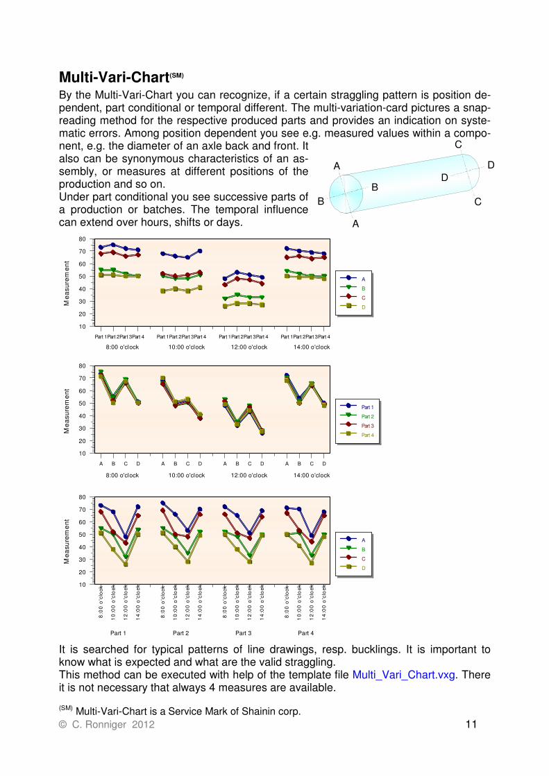
Multi-Vari-Chart(SM) By the Multi-Vari-Chart you can recognize, if a certain straggling pattern is position de-pendent, part conditional or temporal different. The multi-variation-card pictures a snap-reading method for the respective produced parts and provides an indication on syste-matic errors. Among position dependent you see e.g. measured values within a compo-nent, e.g. the diameter of an axle back and front. It also can be synonymous characteristics of an as-sembly, or measures at different positions of the production and so on. Under part conditional you see successive parts of a production or batches. The temporal influence can extend over hours, shifts or days.
It is searched for typical patterns of line drawings, resp. bucklings. It is important to know what is expected and what are the valid straggling. This method can be executed with help of the template file Multi_Vari_Chart.vxg. There it is not necessary that always 4 measures are available.
(SM) Multi-Vari-Chart is a Service Mark of Shainin corp.
Part 1Part 2Part 3Part 4 Part 1Part 2Part 3Part 4 Part 1Part 2Part 3Part 4 Part 1Part 2Part 3Part 4
Me
asu
rem
en
t
10
20
30
40
50
60
70
80
A
B
C
D
A B C D A B C D A B C D A B C D
Me
asu
rem
en
t
10
20
30
40
50
60
70
80
Part 1
Part 2
Part 3
Part 4
8:0
0 o
'clo
ck
10
:00
o'c
loc
k
12
:00
o'c
loc
k
14
:00
o'c
loc
k
8:0
0 o
'clo
ck
10
:00
o'c
loc
k
12
:00
o'c
loc
k
14
:00
o'c
loc
k
8:0
0 o
'clo
ck
10
:00
o'c
loc
k
12
:00
o'c
loc
k
14
:00
o'c
loc
k
8:0
0 o
'clo
ck
10
:00
o'c
loc
k
12
:00
o'c
loc
k
14
:00
o'c
loc
k
Me
asu
rem
en
t
10
20
30
40
50
60
70
80
A
B
C
D
8:00 o'clock 10:00 o'clock 12:00 o'clock 14:00 o'clock
8:00 o'clock 10:00 o'clock 12:00 o'clock 14:00 o'clock
Part 1 Part 2 Part 3 Part 4
A
A
B
B
C
C
D
D

12 © C. Ronniger 2012
Paired Comparison
At the pairwise comparison it is a matter of the comparison of discrepancies between characteristics, regardless their quantitative size. Always pair wise so called ”good” and ”bad” parts are compared. Various criterions are fixed, which are entered side by side in a table.
Then the measured values are compared to each other, if they are bigger, equal or smaller. For this the signs <=> have to be entered beside the particular pairs. In the evaluation the sign < gets the value –1, = the value 0 and > the value 1. If you now add up the summation of rows and pictures the absolute values assorted, you get the ranking of the most important influences:
The result shows, which parameter have to be optimized to get a decisive improvement. This method can be executed with help of the template file Paired_Comparison.vxg.
Length a
Length b
Width
Diameter
Weight
Function
Reliability
Pair 1
123
23
11
1
1
3
34.5
125
25
11
2
2
4
36.5
<
<
=
<
<
<
<
Pair 2
122
22
12
1
1
2
35.8
125
25
11
2
2
4
36.5
<
<
>
<
<
<
<
Pair 3
120
20
11
2
1
5
37
126
23
12
1
0
4
34.5
<
<
<
>
>
>
>
Pair 4
119
23
11
2
0
1
37
123
21
11
1
1
2
36
<
>
=
>
<
<
>
Pair 5
123
23
12
2
-1
3
35.8
124
23
12
1
1
4
36.5
<
=
=
>
<
<
<
Le
ng
th a
We
igh
t
Fu
nc
tio
n
Le
ng
th b
Dia
me
ter
Re
lia
bil
ity
Wid
th
Am
ou
nt
of
eq
ua
l d
iffe
ren
ce
s
0
1
2
3
4
5

© C. Ronniger 2012 13
Comparison B vs. C(SM) Often it occurs that you want to compare 2 ”things” e.g. a new product against an old one. There a certain criterion is relevant, which if possible, should be described with a measured value. If you got a number of ”New” and ”Old” or ”B versus C” parts or sys-tems, those are described sequentially after their evaluation. If there for example ever 2 parts, the following sequence could addict: Part Evalua-
tion N 1,2 N 1,1 A 0,9 A 0,8
Here it is provided that the higher evaluation is the better one. At first the result seems to be unique after the resulted sequence. The both new-parts are before the old-parts. But the sequence could also be the same incidentally. For 2 New and 2 Old there are 6 different possibilities in total:
In general the number of possible variants is determined by:
!!
)!(
altneu
altneu
nn
nnVarianten
⋅
+=
So the probability of the result in the first column is 1/6 or 16.667%. With this random sample a proposition should be done about the main unit. For this you establish a null hypothesis, that New in fact is better than Old. The probability that the null hypothesis applies is 100% less the random probability of 16.667% = 83.3%. Similarly, as a signi-ficance level is fixed for statistical tests, here a limiting value of 5% should be valid. Be-cause this exceeds the limiting value with 16.667% widely, the result of the null hypo-thesis is not significant. In principle the significance level should be fixed before. At a sequence, where always all new ones are before the Old ones, you just have to com-pare the reciprocal of number of variants against the fixed significance level. The null hypothesis that New is better than Old, always has to be dismissed, if 100%/variants > significance level. The following table shows the corresponding sample sizes for various significance le-vels, where the null hypothesis should not be dismissed:
N N N A A A N A A N N A A N A N A N A A N A N N
14 © C. Ronniger 2012
Significance- level
Scope N Scope A
0,1% 2 43
0,1% 3 16
0,1% 4 10
0,1% 5 8
0,1% 6 6
1% 2 13
1% 3 7
1% 4 5
1% 5 4
1% 6
5% 1 19
5% 2 5
5% 3 3
5% 4 3
5% 5
10% 1 9
10% 2 3
10% 3 2
10% 4
10% 5
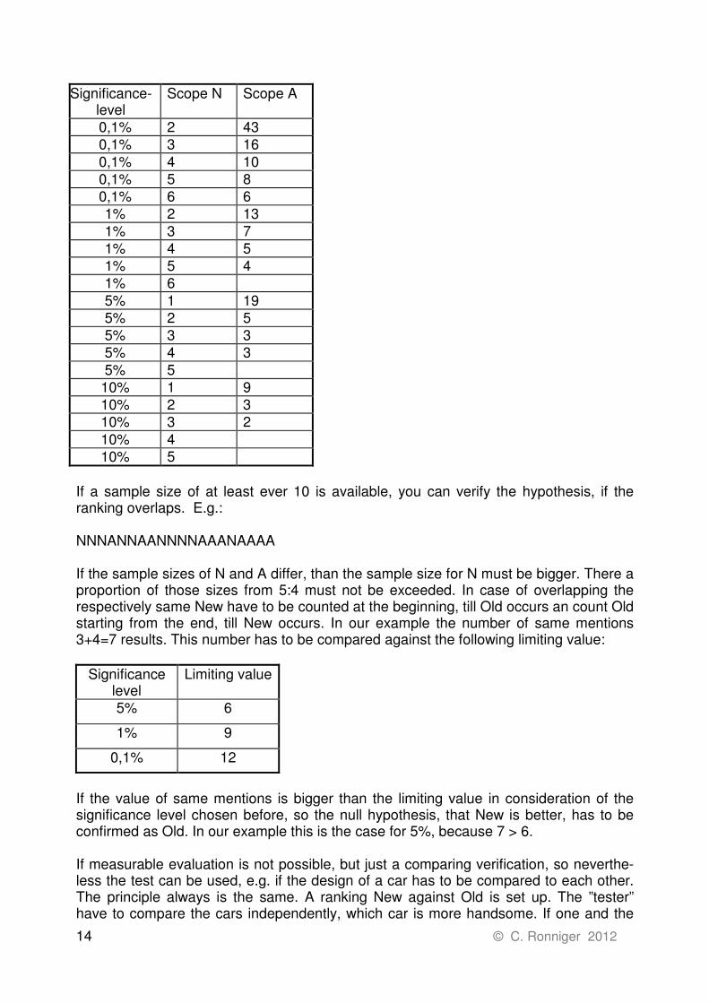
If a sample size of at least ever 10 is available, you can verify the hypothesis, if the ranking overlaps. E.g.: NNNANNAANNNNAAANAAAA If the sample sizes of N and A differ, than the sample size for N must be bigger. There a proportion of those sizes from 5:4 must not be exceeded. In case of overlapping the respectively same New have to be counted at the beginning, till Old occurs an count Old starting from the end, till New occurs. In our example the number of same mentions 3+4=7 results. This number has to be compared against the following limiting value:
Significance level
Limiting value
5% 6
1% 9
0,1% 12
If the value of same mentions is bigger than the limiting value in consideration of the significance level chosen before, so the null hypothesis, that New is better, has to be confirmed as Old. In our example this is the case for 5%, because 7 > 6. If measurable evaluation is not possible, but just a comparing verification, so neverthe-less the test can be used, e.g. if the design of a car has to be compared to each other. The principle always is the same. A ranking New against Old is set up. The ”tester” have to compare the cars independently, which car is more handsome. If one and the

© C. Ronniger 2012 15
same car is named from all 5, then this is the more handsome one under the signific-ance level of 1% fixed before. But if just one makes another choice, the cars are not distinguishable. For this comparison the following limiting values are valid:
Significance- level
Limiting value
5% 3
1% 5
0,1% 6
Also here the test is possible at a quorum of 10 comparisons, if there are different men-tions. The comparative value is calculated from the mentions by 2 * |NamingN – NamingA| Here again the limiting values are valid, like in the measurable evaluation (6-9-12). For the described processes the template Comparison_B_vs_C.vxg has to be used. It is always assumed that independent of the numerical values at the evaluation New must be the ”better” one.
Intensity-Relation-Matrix
In a so called Intensity-Relation Matrix it is the point that the decisive factors for a later investigation should be found, or to reduce the quantity of parameter to the essential ones for an experimental design. At first the entry of factors with their designations takes place vertically in a table. The same factors have to be entered horizontally in the first row. The particular effects of the factors have to be enlisted in the first column on the factors with the same sequence in the first row.
Outside-diameters
Roundness
Plan-sprint
Angle pin
Altitude oil-supply
Scope-situation oil-supply
Height-tolerance
Pin-diameter
1
2
3
4
5
6
7
8
Ou
tsid
e-d
iam
ete
rs
3
0
0
0
3
0
0
Ro
un
dn
ess
3
0
0
1
0
0
0
Pla
n-s
pri
nt
0
0
2
0
0
1
0
An
gle
pin
0
1
0
0
3
0
2
Altitu
de
oil-
su
pp
ly
1
1
2
0
0
1
0
Sco
pe
-situ
atio
n o
il-su
pp
ly
0
0
2
3
0
0
3
He
igh
t-to
lera
nce
2
0
1
0
0
0
0
Pin
-dia
me
ter
0
0
0
2
2
0
0
Passiv-sum
Active-sum

16 © C. Ronniger 2012
Normally the values for this are estimated by experts or specialists. Possibly the numer-ical values can be weighted. In a diagram the active summations are spread over the passive summations after a valuation and parts the diagram shares in four big areas. Those depict the active and passive, as well as the critical and reactive field. For further experimental designs the factors in the active field as well as in the critical field have to be taken into account. Generally here it is a matter of possible reciproca-tions. It is possible to renounce the factors in the passive field. The factors in the reac-tive field can also be performed in the treatment as sub-target factors, which will not be varied in further experimental designs. This method can be executed directly via the menu statistics/Intensity-Relation-Matrix inside the spreadsheet.
Priority Matrix Different criterions or characteristics are compared in the Priority matrix together and a ranking was formed. The result can be used also for importances of the criterions for continuing evaluations No quantitative measurements are necessary for the comparisons of the characteristics. The test is just a pair-wise comparison and an estimation of experts. For example: The importances should be determined for a later comparison of different technical solutions. The characteristics are function, reliability, weight etc. Each criterion has to be compared with each other. That one which is more important gets the number of the criterion (order number in the row). In the first comparison, the function 1 is more important than function 2. Therefore in row 2 of column 1 is the number of function 1. The next step is the comparison of function 1 with the reliability.
Passive sum
0 2 4 6 8
Ac
tive
su
m
0
1
2
3
4
5
6
7
11
2233
44
55
66
77
88
Passive Field Reactive Field
Critical FieldActive Field
Sluggish Reactive
Critical Active

© C. Ronniger 2012 17
Characteristic 1 2 3 4 5 6 7 8 9 10
1 Function1 2 Function2 1 3 Reliability 1 3 4 Weight 1 2 3 5 Required space 1 2 3 5 6 Temperature-constancy 6 6 6 6 6 7 Media-constancy 7 7 7 7 7 6 8 Environment-compatibility 1 2 3 8 8 6 7 9 Montages 1 2 3 4 5 6 7 8
10 Manufacture 1 2 3 4 5 6 7 8 10 11 Costs 1 11 11 11 11 6 7 8 11 11
The column 2 refers on the evaluation of the function 2 opposite each other criterion. The reliability is more important than function 2. Therefore in column 2 is the number of the reliability with the value 3. Now you add up the occurring numbers for each criterion and get the ranking. In this case you can see the following Pareto-Chart.
Each result should be increased of 1, because it is not meaningful to get values with zero (if the results are importances and you multiply this with other evaluations, you will get also zero), the other point is that in the Pareto-Chart a zero value is not visible. This method can be executed with help of the template file Priority_Matrix.vxg
Te
mp
.-c
on
sta
nc
y
Me
dia
-co
ns
tan
cy
Fu
nc
tio
n1
Re
lia
bil
ity
Co
sts
En
vir
.-c
om
pa
tib
ilit
y
Fu
nc
tio
n2
Re
qu
ire
d s
pa
ce
We
igh
t
Ma
nu
fac
ture
Mo
nta
ge
s
Pri
ori
ty
0
2
4
6
8
10
12

18 © C. Ronniger 2012
Matrix diagram The so called “matrix diagram” is just a representation of a matrix, not really a diagram. However, through an assessment of the rows and columns between each other, there is built a structure. In the following example the task is to show which method (the first column) is suitable for which use case (the first line).
It is possible to use other items, titles or meaning. The mutual relations are described here as numerical values between 1 and 3. No connection means empty fields or 0. Leaving out 0 has the big advantage that the representation becomes more clear (pat-tern). Note: The difference is to intensity relation matrix is the titles of the first row are identical with the first column (mutual comparison). Another evaluation is possible by the row-by-row summation (who brings most points).
to find
ideas
prese
nt in
form
ations
data
colle
ction
data
eva
luat
ion
stru
ctur
ing
illus
trate
pro
cess
es
proce
ss capa
bility
proc
ess co
ntrol
illustra
te con
nect
ions
syst
em a
nalysis
conc
ept -
design
failu
re cau
se
Brainstorming 3 1 2 3 1
Monitor, count, measure 3 2
Correlation-diagram 3 2 2 3
Regression/Model-charts 3 3 3 3
Cause-effect-diagram 3 3 2 3 3 3 3
Block-diagram 3 3 1 2 2 3 1
Flow-chart, process-chart 3 3 3 3 3 2
Intensity-relation-matrix 3 2 2 3 2 2
Matrix diagram 3 1 2 3 2 2 1
Priority-evaluation 3 2 2 3 2
Pareto-analysis 2 2 2
Paired comparison 2 1 2 3 2
Histogram 3 3 1 2 1
Quality chart 2 2 2 3
Probability chart 2 2 3 2
Weibull 2 2 1 2
3 2 2

© C. Ronniger 2012 19
2. Analysis of Variance (ANOVA)
Basics
In the Variance Analysis (Aanalysis of Variance) the target is to evaluate the variances of groups (factors) compared with the unexplained variance (rest scatter) and of con-firming a significant influence or effect. The suitable analysis of scatter is a sum of:
total differences = differences of factors + unexplained scatter
ErrorFactorsTotal SSSSSS +=
SS = Sum of Squares
( ) ( ) ( )2
1 1
2
1
2
1 1
∑∑∑∑∑= === =
−+−=−z
j
n
i
jji
z
j
j
z
j
n
i
ji yyyyyy
The variances are built with the “degrees of freedom” in the denominator:
z = number of factors, n = number of measurements (rows)
The quotient MSFactors/MSError builds the so called F – value for the test statistics (test of mean effects).
Error
Factors
MS
MSF =
The greater the F-value is, the likelyhood for the effect of the factor is the higher. The null-hypothesis Ho is: The means between the factors are equal. Ho will be rejected if F < Fz-1; z(n-1);α One distinguishes an ANOVA between two or several factors (data rows).
j = index of columns i = index of rows
−⋅=
−=
−⋅=
)1(11 nz
SSMS
z
SSMS
nz
SSMS Error
ErrorFactors
FactorsTotal
Total

20 © C. Ronniger 2012
ANOVA between two Series In the analysis of variance a significant difference should be determined between two test series. In an example it should be determined, if the body height between Europe-ans and Africans is different. There are following data:
Europeans
Africans
159 187 163 173 156 177 173 181 161 169
First the the square sum of variances for the average is formed, which corresponds to the so called correction factor.
( )CF
n
DataDataSQA
tot
m =+
= ∑∑2
21
with ntot = number of measures Data1 and Data2 Afterwards the total of squared variances is determined:
CFDataDataGSQii
−+= ∑∑22
21
with the belonging degree of freedom DF = ntot-1 Furthermore the total of squared variances of the single data arrays have to be formed
( ) ( )CF
n
Data
n
DataSQA −+= ∑∑
2
2
1
221
with degree of freedom DFA = 1 The square total of the error is calculated by:
SQAGSQSQF −= with degree of freedom DFF = ntot -2 Variances are determined accordingly:
F
F
A
ADF
SQFV
DF
SQAV ==
The so called F-value is the quotient of the both variances

© C. Ronniger 2012 21
F
A
V
VF =
which is compared to a critical F-value Fkrit on a fixed level of significance, e.g. 95%. If F > Fkrit, DFA, DFF, it means that both series are significantly different. The percental share in the total effect is calculated by
FA VDFSQASQA ⋅−='
%100'
GSQ
SQAA =
and describes the average effects. The difference to 100% corresponds to the share of errors This procedure can be used with the submission file ANOVA_Two_Samples.vxg in di-rectory \Statistics See also : ANOVA & ANOM with several Factors

22 © C. Ronniger 2012
ANOVA & ANOM with several Factors In the analysis of variance with several factors the influences of test parameters are tested on a target size. It should be find out, which influence do the parameter have on the test result propor-tional to the dispersions. After analysis of variance it is issued by the statistical F-Test , if the parameter does have a significant influence and how great it’s percentage share is compared to the re-maining dispersion. It is assumed that the deviations are normal distributed. Otherwise the result is not unique. In the following example the depicted trials are executed.
Target size Temperature
Print Set up ti-me
Cleaning
1 -20 1 1 1 1 2 -10 1 2 2 2 3 -30 1 3 3 3 4 -25 2 1 2 3 5 -45 2 2 3 1 6 -65 2 3 1 2 7 -45 3 1 3 2 8 -65 3 2 1 3 9 -70 3 3 2 1
The single steps of ANOVA: 1) Formation of square total of deviations for the mean value, which is also indicated as correction factor
CFYn
SQMn
i
i =
= ∑
=
2
1
1
2) Formation of square total of deviations of the total mean value
∑=
−=n
i
i CFYGSQ
1
2
3) Formation of total of the squared deviations regarding the factors
( ) ( ) ( ) CFYn
Yn
Yn
SQA AA
AA
AA
A −++= ∑∑∑2
22
22
2
21
1
111
whereby nA1, nA2 and nA3 at each case is the number of points of similar adjustments for A and in our example A stands for temperature. For B (print) counts analogous:

© C. Ronniger 2012 23
( ) ( ) ( ) CFYn
Yn
Yn
SQA BB
BB
BB
B −++= ∑∑∑2
22
22
2
21
1
111
( ) ........1 2
11
+= ∑ CC
C Yn
SQA
and so on. 4) Estimation of variances of single factors as quotient from the squared deviation to the degree of freedom
A
A
ADF
SQAV =
B
B
BDF
SQAV = ....=CV .... .....
whereby DF = number of steps –1 (number of independent settings, which can still be changed starting from a step, in the example DFA = 2 ). 5) Determination of error variance In general at examination of experimental designs two types of errors can occur: F1 = error within a characteristic combination, whereby this should be 0 at correspond-ing carefulness of execution. F2 = error at repeating of measurings The variance of error F2 can be estimated according to following rule: you contract the square total of factors with the least squared deviations, in our example SQAC+D = 400. Approximately half the number of DF’s should be used. Thus the error variance results by
DC
DC
FDF
SQAV
+
+=2
6) Calculation of proportion of factor variances to error variance
2F
AA
V
VF =
2F
BB
V
VF = ......=CF
7) Determination of significance of the corresponding factors The prior determined F-value can be compared to a critical F-value. The null hypothesis is set up FA > Fkrit, there is a significant difference with x % . The critical F-value, e.g. for A you get from F-tables with degree of freedom f1= DFA = 2 and f2 = DFC+D = 4 and a level of significance of 95%. 8) Percental meaning of a factor An important result of the analysis of variance is the percental share of a factor on the target size. This is determined e.g. for A by:

24 © C. Ronniger 2012
2' FAAA VDFSQASQA −=
%100'
GSQ
SQAA A
A =
The percental share of F2 is determined by:
%100222
GSQ
VSQAA FF
F
−=
For the example in total there are following results:
Consequently the critical influence is the temperature. In the so called ANOM (Analyis Of Means) the mean values of target sizes of each ad-justment of each factor are depicted. For the example described in the ANOVA following description arises:
For the described procedure the submission ANOVA_MultiFactors.vxg in the directory \Statistics has to be used. If several measurings are used for each factor adjustment, so the lot fraction defective has not be estimated with the smallest factor shares, but can be determined directly. First of all a square total is calculated for the error:
Temperature
Pressure
Time
Cleaning
Error 2
DF
2
2
2
2
4
SQA
2450
950
350
50
400
V
1225
475
175
25
100
F
12.25
4.75
1.75
0.25
SQ'
2250
750
150
Percent %
59.2
19.7
3.9
7.9
F critical
6.94
6.94
6.94
6.94
A1 A2 A3 B1 B2 B3 C1 C2 C3 D1 D2 D3
Re
sp
on
se
-60
-50
-40
-30
-20
Temperature
Pressure
Time
Cleaning

© C. Ronniger 2012 25
∑=
−=p
i
iF SQAGSQSQA
1
2 with p = number of factors
and the variance is:
)1()1(2
2
22 −−−⋅== nnnyf
DF
SQAV F
F
F
F
with ny = number of repetitions, n = number of trials The relative shares are determined analogous to the previous approach via:
2
'
Fxxx VDFSQASQA ⋅−=
%100'
GSQ
SQAA
xx =
For the ANOVA with repetitions the submission ANOVA_MultiFactors_Repetition.vxg in directory \Statistics has to be used. See also: ANOVA between two Series
26 © C. Ronniger 2012
3. Design of Experiment
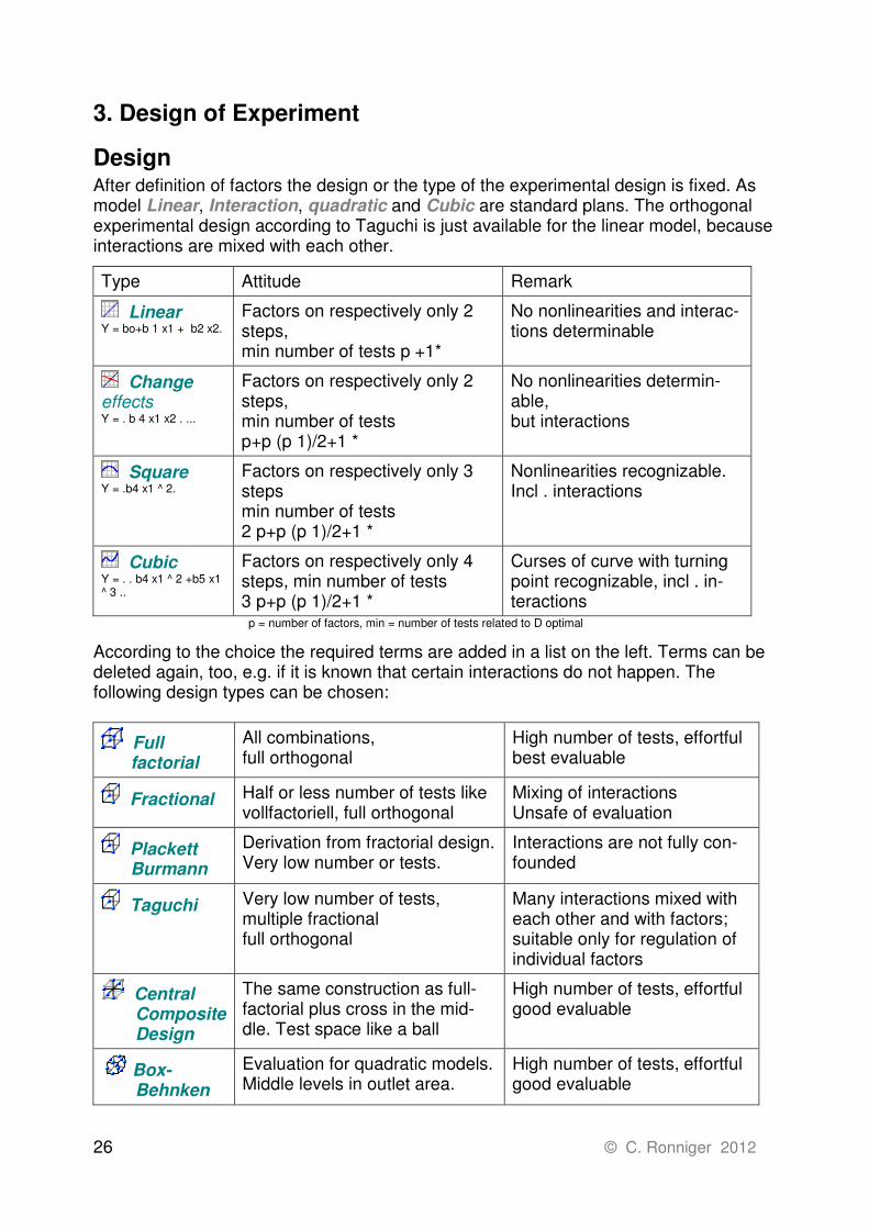
Design After definition of factors the design or the type of the experimental design is fixed. As model Linear, Interaction, quadratic and Cubic are standard plans. The orthogonal experimental design according to Taguchi is just available for the linear model, because interactions are mixed with each other.
Type Attitude Remark
Linear Y = bo+b 1 x1 + b2 x2.
Factors on respectively only 2 steps, min number of tests p +1*
No nonlinearities and interac-tions determinable
Change effects Y = . b 4 x1 x2 . ...
Factors on respectively only 2 steps, min number of tests p+p (p 1)/2+1 *
No nonlinearities determin-able, but interactions
Square Y = .b4 x1 ^ 2.
Factors on respectively only 3 steps min number of tests 2 p+p (p 1)/2+1 *
Nonlinearities recognizable. Incl . interactions
Cubic Y = . . b4 x1 ^ 2 +b5 x1 ^ 3 ..
Factors on respectively only 4 steps, min number of tests 3 p+p (p 1)/2+1 *
Curses of curve with turning point recognizable, incl . in-teractions
p = number of factors, min = number of tests related to D optimal
According to the choice the required terms are added in a list on the left. Terms can be deleted again, too, e.g. if it is known that certain interactions do not happen. The following design types can be chosen:
Full factorial
All combinations, full orthogonal
High number of tests, effortful best evaluable
Fractional Half or less number of tests like vollfactoriell, full orthogonal
Mixing of interactions Unsafe of evaluation
Plackett Burmann
Derivation from fractorial design. Very low number or tests.
Interactions are not fully con-founded
Taguchi Very low number of tests, multiple fractional full orthogonal
Many interactions mixed with each other and with factors; suitable only for regulation of individual factors
Central Composite Design
The same construction as full-factorial plus cross in the mid-dle. Test space like a ball
High number of tests, effortful good evaluable
Box- Behnken
Evaluation for quadratic models. Middle levels in outlet area.
High number of tests, effortful good evaluable

© C. Ronniger 2012 27
D-Optimal Very low number of tests, Clear regulation of interactions,
not orthogonal good evaluable
Mixture Use of factors whose sum must always amount to 100%
not orthogonal, factors de-pendent on each other good evaluable
Coexistent with the model and type selection the number of so called candidates and the number of needed trials is shown beneath. The candidates always correspond to those of the full factorial experimental design. So for a squared model with 3 factors 3^3=27 trials are needed. In addition also a central point with the middle values and re-peats can be chosen. For this see options.
Full-, fractional and Taguchi experiments Full factorial A vollfaktorieller test plan is made if all possible atti-tudes of the factors are combined with each other. The number of tests required can be calculated through:
pn 2= At 3 factors, 8 tests arise. Simply one gener-ally prepares a full facto-rial plan (-1 and 1 stan-dardize) in the following way: It is the advantage of the complete test plan that all inter-actions can be explained. So the influence of A*B*C is just as contained. The number of tests increases with the number of factors, however, very strongly fast, so that the test plan gets too effortful beginning at 5 factors. The question how one can simplify it arises. This plan is full orthogonal
Fractional The triple interaction has only a small influence in most cases. Concerning this statement, one can put another factor instead of the combination which contains A*B*C and then one receive a fractional test plan. In this case the plan is the half size of the full-factorial plan with 24-1. It is the disadvantage of this test plan that no more triple interactions are
A B C D E F
1 -1 -1 -1 -1 -1 -1
2 1 -1 -1 -1 -1 -1
3 -1 1 -1 -1 -1 -1
4 1 1 -1 -1 -1 -1
5 -1 -1 1 -1 -1 -1
6 1 -1 1 -1 -1 -1
7 -1 1 1 -1 -1 -1
8 1 1 1 -1 -1 -1
9 -1 -1 -1 1 -1 -1
10 1 -1 -1 1 -1 -1
11 -1 1 -1 1 -1 -1
12 1 1 -1 1 -1 -1
13 -1 -1 1 1 -1 -1
14 1 -1 1 1 -1 -1
15 -1 1 1 1 -1 -1
16 1 1 1 1 -1 -1
17 -1 -1 -1 -1 1 -1
18 1 -1 -1 -1 1 -1

28 © C. Ronniger 2012
determinable and two-factor interactions are confounded with each other: AB with CD, AC with BD and AD with BC, because the respective column products are identical. For a product with at least 4 columns, e.g. F=ABCD two-factor interactions aren't con-founded any more. These plans have a so-called resolution of at least V. In general the number of tests is calculated through
12 −= pn
One build this factorial design at first like the full-factorial plan, but with q factors less. The attitudes of the missing factors q are generated by the product of all previous col-umns. One also calls these columns "generators". The following table shows an over-view for 12 factors:
n p 2 3 4 5 6 7 8 9 10 11 12
4 22 fullfact.
23-1
III
8 23 fullfact.
24-1
IV 25-2
III 26-3
III 27-4
III
16 24 fullfact.
25-1
V 26-2
IV 27-3
IV 28-4
IV 29-5
III 210-6
III 211-7
III 212-8
III
32 25 fullfact.
26-1
VI 27-2
IV 28-3
IV 29-4
IV 210-5
IV 211-6
IV 212-7
IV
64 26 fullfact.
27-1
VII 28-2
V 29-3
IV 210-4
IV 211-5
IV 212-6
IV
128 27 fullfact.
28-1
VIII 29-2
VI 210-3
V 211-4
V 212-5
IV
Fullfactorial -> all interactions are evaluable
Fractional plans -> all two-factor interactions evaluable ≥ V
Fractional plans -> two-factor interactions mixed, resolution < V
All fractional plans with resolution V or more are uncritically in the evaluation. Also here the effort rises up excessive over a number of 6 factors. Therefore D-optimal test plans at which all interactions can always be found out then can be recommended. Plans with resolution less than V gets smaller size but can be used only for searching the most important factors, because interactions are confounded. One also calls this Screening.
Resolution III Design Main effects are confounded (aliased) with two-factor interactions.
Resolution IV Design No main effects are aliased with two-factor interactions, but two-factor interactions are aliased with each other.
Resolution V Design No main effect or two-factor interaction is aliased with any other main effect or two-factor interaction, but two-factor interactions are aliased with three-factor interactions. With using D-Optimal plans there is still the chance to determine all interactions by the same size of trials like for resolutions < V (see the following chapters).

© C. Ronniger 2012 29
Plackett-Burman-experiments Especially Plackett-Burman-Experiments are suitable for preliminary investigations or so-called Screening-plans (only 2 levels). These test plans are derived from fractional plans and can be constructed in steps by 4 tests. With 12 tests there can be determined 11 effects (factors). Nevertheless, it is recommended not to use at least two columns with factors. Plackett Burman-test plans have compared with the classical fractional plans (resolution III) the greate advantage that interactions among each other and with other factors are not completely confounded. For plans with 12 tests and 11 factors a max. correlation of 0,333 arises for two-factor interactions. An evaluation via multiple regression is here normaly not a problem. For plans with 20 tests and 19 factors a max. correlation of 0,6 exists. This can be critical to determine interactions. Under circumstances this correla-tion is too high for evaluations of interactions, in particular if high scatter are given. In-deed, an additional security is given by the evaluation with the method PLS which is non sensitive against correlations. But there are in each case no confoundings between the factors. After evaluation with the stepwise regression ordinarily fall out a greate number of 2-factor interactions. Plackett Burman-test plans thereby advantageous when an evalua-tion should be done before of unknown interactions, but the test expenditure must be very small. Confirmation tests are to be recommended, in any case. The creation of the plans occurs through the following pattern: A combination order which is repeated column for column around a line down moved is used in each case. The pattern is depending on n:
n=12 + + - + + + - - - + -
n=20 + + - - + + + + - + - + - - - - + + -
n=24 + + + + + - + - + + - - + + - - + - + - - - -
The last field is absent. After cyclic joining together of the columns the surpluses about the line n-1 are added on top again. The last missing line is taken with continuously -1.

30 © C. Ronniger 2012
Orthogonality All full-factorial and fractional plans are orthogonal. If there are the factors independent from each other and the correlation coefficients are 0, the plan is full orthogonal. Every factor can have values without changing the attitudes of the other factors. This isn't the case in the right representation. B cannot be changed independently by A. If the plan is not quite orthogonal, e.g. due to a central points, then the evaluation is still possible with the calculation via matrices. At the same deviation of the Y values, the confidence inter-vals are, however, wider than at orthogonal plans.
Taguchi Taguchi plans are, fractional test plans which still more interactions are covered with factors. e.g:
472 −
Through this one needs a very low number of tests. A mixture of factors with interaction also arises from it. Therefore these plans only are recommended if interactions cannot be expected. This plan is full orthogonal. The plans are marked by Lx in which x is the number of test. These plans are appropriately orthogonal. 2 examples of orthogonal combi-nations to Taguchi represent the following plans: Instead of the standardization -1 ... 1 the attitudes are numbered
L4 (23)L4 (23)
L9 (34)L9 (34)
A B
C
- 1
1 1
1
A B
C
-1
11
1orthogonal not orthogonal
© C. Ronniger 2012 31
real curve
curve of quadr. model
fictitious minimum
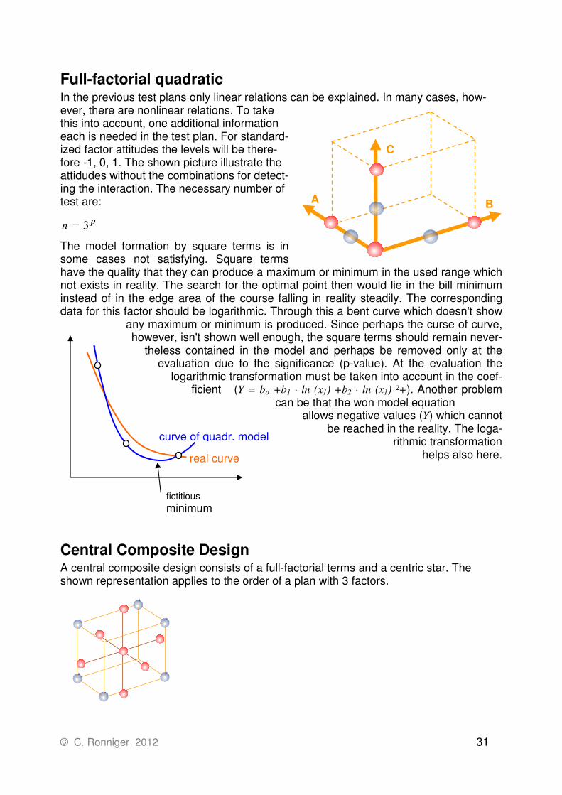
Full-factorial quadratic In the previous test plans only linear relations can be explained. In many cases, how-ever, there are nonlinear relations. To take this into account, one additional information each is needed in the test plan. For standard-ized factor attitudes the levels will be there-fore -1, 0, 1. The shown picture illustrate the attidudes without the combinations for detect-ing the interaction. The necessary number of test are:
pn 3=
The model formation by square terms is in some cases not satisfying. Square terms have the quality that they can produce a maximum or minimum in the used range which not exists in reality. The search for the optimal point then would lie in the bill minimum instead of in the edge area of the course falling in reality steadily. The corresponding data for this factor should be logarithmic. Through this a bent curve which doesn't show
any maximum or minimum is produced. Since perhaps the curse of curve, however, isn't shown well enough, the square terms should remain never-
theless contained in the model and perhaps be removed only at the evaluation due to the significance (p-value). At the evaluation the
logarithmic transformation must be taken into account in the coef-ficient (Y = bo +b1 · ln (x1) +b2 · ln (x1) ²+). Another problem
can be that the won model equation allows negative values (Y) which cannot be reached in the reality. The loga-
rithmic transformation helps also here.
Central Composite Design A central composite design consists of a full-factorial terms and a centric star. The shown representation applies to the order of a plan with 3 factors.
A B
C
32 © C. Ronniger 2012
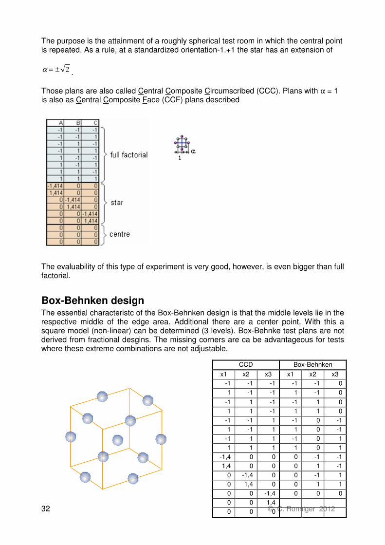
The purpose is the attainment of a roughly spherical test room in which the central point is repeated. As a rule, at a standardized orientation-1.+1 the star has an extension of
2±=α .
Those plans are also called Central Composite Circumscribed (CCC). Plans with α = 1 is also as Central Composite Face (CCF) plans described
The evaluability of this type of experiment is very good, however, is even bigger than full factorial.
Box-Behnken design The essential characteristc of the Box-Behnken design is that the middle levels lie in the respective middle of the edge area. Additional there are a center point. With this a square model (non-linear) can be determined (3 levels). Box-Behnke test plans are not derived from fractional desgins. The missing corners are ca be advantageous for tests where these extreme combinations are not adjustable.
CCD Box-Behnken
x1 x2 x3 x1 x2 x3
-1 -1 -1 -1 -1 0
1 -1 -1 1 -1 0
-1 1 -1 -1 1 0
1 1 -1 1 1 0
-1 -1 1 -1 0 -1
1 -1 1 1 0 -1
-1 1 1 -1 0 1
1 1 1 1 0 1
-1,4 0 0 0 -1 -1
1,4 0 0 0 1 -1
0 -1,4 0 0 -1 1
0 1,4 0 0 1 1
0 0 -1,4 0 0 0
0 0 1,4
0 0 0

© C. Ronniger 2012 33
Box-Behnke test plans can be turned approximately. Under 45° one identify in the pic-ture on top a CCD plan. In the left table a Box Behnke design (not rotated) is compared with the CCD- design. In the Box-Behnke design a little bit fewer tests are required. If one used in the CCD plan correct-wise 3 central points, the difference precipitates even greater.
D-Optimal experiments Fundamentals The aim of D-Optimal plans is with minimum effort to prepare test plans which show the desired effects and interactions definitely. This is, a decisive advan-tage over the fractorial design where interactions are confounded with each other partly. with p = number the number of simple interactions charges itself to factors: p’ = p*(p-1)/2 As a rule, the higher interactions (e.g. ABC, ABD, ACD etc.) are not taken into account since its influence is usually less opposite the simple ones. You also would blow up the size of the tests. Altogether, the following number of tests is needed for a test plan with two attitudes: Constant : 1 Main effects (factors) : p Interactions : p’ = p*(p-1)/2 Sum : p+ p*(p-1)/2+1 In the case of a square model there are still one time p tests (with a middle attitude). Furthermore gets approx. . 5 tests needs to receive sufficient information about the spreads (significances of the factors). A D-Optimal plan is not generated with a firm scheme but built up iteratively. It has among others the following important qualities:
• Maximization of the determinant (indicator for evaluability)
• Minimization of the correlations and confidence intervals
• Balanced levels( as good as possible) Due to the target that all interactions shall be recognized at a low test number prevents particularly that these plans are orthogonal completely ., i.e. certain correlations cannot be removed completely. This is, however, a subordinate disadvantage in the evaluation about Multiple Regression.

34 © C. Ronniger 2012
Advantages of the D-Optimal test plans
• Free choice for the number of the steps per influence factor. The number of lev-els can be elected factor by factor differently.
• Free choice of the step distances which can equidistantly or not be chosen equi-distantly.
• Free choice for the distribution of the test points in the n dimensional test room
• Free choice of the mathematical model
• Expansion capability by new influence factors
• Certain attitudes and combinations can be excluded, these are not attainable
Disadvantages of the D-Optimal test plans
• The test plan is not orthogonal, however, the deviations are usually only small
Mixture experiments Being indicated in the shares in % at experiments at which it e.g. is about mixtures from chemical liquids. The factors are what in normal test plans, are the different components in mixture plans. All shares must show in sum 100% what leads to the following term x1 + x2 + ... xk = 1 k = count of components and mean that the components are dependent on each other. This e.g. must be taken into account for the respective tests and can't be treated by standard test plans (only with effort). The possible quota combinations lie in an equilateral triangle. In most cases there are 3 components. The corresponding test plan looks like repre-sented on the right in comparison with the "conventional" one:
Full factorial Mixed
Combinations must be within the range represented grayed. At k=4 components = the possible combinations lie in a tetrahedron. Simplexe are called triangle, tetrahedra and the corresponding arrangements at more than 4 components, the mixture plans are therefore also described as a simplex-plans. For the regulation of only the "main effects" a plan is a so-called type "grade 1" uses. This corresponds to a linear test plan.
A B
C
A B
C
1,0,0 0,1,0
0,0,1

© C. Ronniger 2012 35
A test plan of the type grade 2 shows the following combinations (in addition with use of all components in the last line):
Interactions and nonlinearities can hereby be detected. The next level is grade 3, what is shown in the following table:
No. comp. A comp. B comp. C 1 1 0 0 2 0 1 0 3 0 0 1
No. comp. A comp. B comp. C 1 1 0 0 2 0 1 0 3 0 0 1 4 1/2 1/2 0 5 0 1/2 1/2 6 1/2 0 1/2 6 1/3 1/3 1/3
Nr. comp. A comp. B comp. C 1 1 0 0 2 0 1 0 3 0 0 1 4 1/3 2/3 0 5 2/3 1/3 0 6 0 1/3 2/3 7 0 2/3 1/3 8 1/3 0 2/3 9 2/3 0 1/3
10 1/3 1/3 1/3

36 © C. Ronniger 2012
With increasing factors and grade the number of tests increases fast as the following table points:
compon. Grade 1 Grade 2 Grade 3 Grade 4 2 2 3 4 5 3 3 6 10 15 4 4 10 20 35 5 5 15 35 70 6 6 21 56 126 7 7 28 84 210
Number of tests into dependence of the number of components and of the type
General is the formula
g
gkkkkm
......321
)1)....(2)(1(
⋅⋅++++
=
k = number factors, g = grade
To limit the effort, one uses also here D-Optimal. The procedure is comparable with the conventional plans why be further come in here on this shall not. The evaluation of mixture plans is carried out with the help of the multiple regression. grade 1 corresponds to the model linear, grade 2 squarely etc. The condition x1+ x2+.. xk = 1 is the reason, however, that some of the coefficients gen-erally approach disappear. But the evaluation can be done via Neural Network anyway.

© C. Ronniger 2012 37
Comparision of Designs
Full
factorial
Fractional Plackett-
Burman
Taguchi CCD D-Opt.
orthogonal ���� ���� ���� ���� ���� –
quadratic ���� – – partly ���� ����
cubic ���� – – partly ���� ����
Inter-
actions ����
partly type
IV or type V+
partly by
enoughDF
– depends
on basis ����
Numberexperiments
verylarge
middle little verylittle
largelittle
partly eval.
previously– – – – ���� –
contrainspossible
– – – – – ����
all
combinationsincl. 3- IA
all
2- IA_Resolution V+
less
unknownIA
no IA
expected
Full-factorial
Fractionalfactorial
Plackett-Burmann
TaguchiLn(2p)
TaguchiLn(3+
p)
no IA
expected
certain
or all IA
CCDCCF
evaluation
2 levelspreviously
D-Optimal
not all
combinationspossible
3 Levelsnon lin.
2 Levelslinear
2nd step, extended DoE
IA Abbreviation for Interaction

38 © C. Ronniger 2012
Correlation If a connection exists between different factors (dataset), the degree or the strength of this connection can be ascertained with the correlation.
Correlation coefficient after Bravais - Pearson The measurement of the degree of this connection is the correlation coeffizicient r. For two dataset x and y, r is calculated after Bravais - Pearson with:
( )( )( )( ) ( )∑ ∑∑
−−
−−==
22yyxx
yyxx
ss
sr
ii
ii
yx
xy
xy
With the help of the t-test the hypothesis can be checked: x and y can be considered as two independent datasets. The test statistic is:
21 2
−−
= nr
rt
xy
xy
pr
The hypothesis on independence is rejected, if
2/1,2 α−−> npr tt
The correlation coefficient after Bravais-Pearson strongly reacts to outliers in the obser-vations. Hence, the dataset should be normally distributed.
Rank correlation - Spearman If the dataset is strongly non normally distributed or if there ar categorial attributes, the rank correlation has to be used. Instead of the values the ranking of the sorted data is used. For example for x = [5;2;7;4] the rank of the value 5 is R=3. The Spearman corre-lation coefficient is calculated with:
( )
)1(
)()(6
12
1
2
−
−−=∑
=
nn
yRxR
r
n
i
ii
s
Also here the t-test is used to check if the datasets x and y can be considered as two independent datasets. For normally distributed data the difference between Bravais-Pearson and Spearman is low.
© C. Ronniger 2012 39
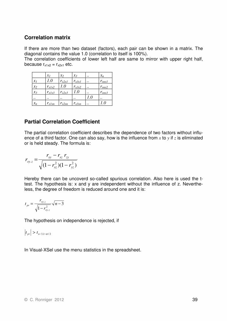
Correlation matrix If there are more than two dataset (factors), each pair can be shown in a matrix. The diagonal contains the value 1.0 (correlation to itself is 100%). The correlation coefficients of lower left half are same to mirror with upper right half, because rx1x2 = rx2x1 etc.
Partial Correlation Coefficient The partial correlation coefficient describes the dependence of two factors without influ-ence of a third factor. One can also say, how is the influence from x to y if z is eliminated or is held steady. The formula is:
)1)(1( 22.
yzxz
zyxzxy
zxy
rr
rrrr
−−
−=
Hereby there can be uncoverd so-called spurious correlation. Also here is used the t-test. The hypothesis is: x and y are independent without the influence of z. Neverthe-less, the degree of freedom is reduced around one and it is:
31 2
.
. −−
= nr
rt
zxy
zxy
pr
The hypothesis on independence is rejected, if
2/1,3 α−−> npr tt
In Visual-XSel use the menu statistics in the spreadsheet.
x1 x2 x3 .. xn
x1 1.0 rx2x1 rx3x1 .. rxnx1
x2 rx1x2 1.0 rx3x2 .. rxnx2
x3 rx1x3 rx2x3 1.0 .. rxnx3
.. .. .. .. 1.0 ..
xn rx1xn rx2xn rx3xn .. 1.0

40 © C. Ronniger 2012
4. Regression
General If there is a connection between different features, then the degree or the strength of this connection can be determined with the help of correlation. The correlation coeffi-cient r describes the strength of the connection. One tries at the regression calculation to put a line or curve adapted to the measure-ment pairs optimally. This is a compensation straight line in the simplest case at linear slope. One understands the determination of the coefficients of the compensation straight line by an optimal customization in that way that this differences of the straight line becomes a minimum (least square method). The correlation coefficient expresses how good the found equation adapts to the measurements. The nearer r is due to 1, the better the precision is. In any case there must be always more data than model coeffi-cients exists. There is not always a linear connection. The main problem of the regression calculation is to find the right function. At the choice of the suitable function for the regression one should therefore watch the course of the measurements exactly at first and re-gard maybe known physical dependencies.
Linear Regression
The linear regression is defined through:
xbaY += The gradient b and the section of the straight lines by the y-axis a is calculated through:
( )( )
( )xbya
xx
yyxx
bn
i
i
n
i
ii
−=−
−−=
∑
∑
=
=
1
2
1
The confidence interval for the expected value iy at the position xi is calculated through
the min und max-value:
CxbaYCxbaY ioiu ++=−+=
with
( )
( )∑=
−−
−
−+=
n
j
j
i
n
xx
xx
ntsC
1
2
2
2/1,2
1γ
The estimated standard deviation s is calculated from the variance by the deviations of the observations to the compensation straight line:
( )∑=
+−=n
i
ii xbaYs1
2)(²

© C. Ronniger 2012 41
Each position of xi results a different wide confidence bounds along the straight line de-finded through:
CxbaYunten −+= and CxbaYoben ++=
which is at least at xxi = :
cm
Körpergröße
5 10 15 20 25 30 35
kg
Ge
wic
ht
-0.2
0.0
0.2
0.4
0.6
0.8
1.0
1.2
Linear regression through 0-point
In certain cases the facts force, that the compensation straight goes by the 0 point.
The standard equation xbaY += becomes:
∑
∑
=
===n
i
i
n
i
ii
x
yx
bmitxbY
1
2
1
Size
We
igh
t
with

42 © C. Ronniger 2012
Nonlinear regression
A nonlinear curve is for example xb
eaY = . The standard deviation is here:
( )∑=
−=n
i
iixb
eaYs1
2
²
C is calculated like by the linear regression. The confidence interval is adequate:
Cxb
unten eaY−= and Cxb
oben eaY+=
For example:
Monate
Alter Fzg
5 10 15 20 25 30 35
Ste
igu
ng
b
0.5
1.0
1.5
2.0
2.5
3.0
Regression types Under the button Regression in the dialogue window Diagram types find the following represented functions, where it is up to 7 degrees possible for polynoms
Y = a x^b Straight line in a double logarithm scale Y = a + b·x Simple straight line Y = a + b·x + c·x
²
Y = a + b·x + c·x² + d·x
³
Y = a + b·x + c·x² + ... Polynom up till 7th grade
Y = a·e^(b·x) Y = a·e^(b/x) Y = a + b/x Y = a + b·log(x) Straight line in a single logarithm scale
X
Y

© C. Ronniger 2012 43
To find the right function choice the following examples of the most important types are shown below (coefficients -1 …. +1):
Courses which have a maximum or a minimum happen frequently. An typically function with a minimum in point 0 is Y=X² . If there are data points which goes not through the
Y x2
=
-4 -2 0 2 4
-10
-5
0
5
10
Y x x2
+ x3
+=
-4 -2 0 2 4
-10
-5
0
5
10
Y1
x=
0 1 2 3 4
0
1
2
3
4
5
Y e
1
x=
0 1 2 3 4
0
2
4
6
8
10
Y ex-
=
0 1 2 3 4
0.0
0.2
0.4
0.6
0.8
1.0
Y ex
=
-4 -2 0 2 4
0
1
2
3
4
5

44 © C. Ronniger 2012
0-point, there must be an offset like Y=X²+b. A regression of a parabola determines this offset b automatically. If the minimum is on the right or on the left of the Y-axis the pa-rabola fails. The x-data column has to be moved to the y-axis necessarily around the value of the moving. For 3D-charts with two independent variables x and z the following basic functions are available: Y = a + b·x + c·z
Y = a + b·x + c·z²
Y = a + b·x² + c·z
Y = a + b x² + c·z² The functions produced after the regression with concrete coefficients are in the For-mula linterpreter and can be changed afterwards. Perhaps this makes sense if single coefficients from other experiences are known. In this case there is no longer connec-tion to the previous found coefficients

© C. Ronniger 2012 45
Multiple Regression One uses a multiple regression if more than one independent factor x is available. The simple linear model is: y = b0 + b1 x1 + b2 x2 + b3 x3 + ....
It is presupposed that the features are normal distributed and linear. E.g. not linear pa-rameters can be realized in most cases by remodelling or by using squared terms: y = b0 + b1 x1 + b2 x1² + b3 x2 + ....
In case of tabular values this means that one adds the column to x with the values in a new column copied and squared. E.g. a combination two influences which represents an interaction also can be carried out: y = b0 + b1 x1 + b2 x1 x2 + b3 x2 + ....
The corresponding table columns for x then have to be inserted in a new column as a product x². Further conversions are possible to reach the linear model. In matrix form the model equation is:
Xby =ˆ
with y = vector of the results from the parameter set X = matrix of the actual parameter values b = vector of the coefficients
=
=
=
z
o
znn
z
z
n b
b
b
b
xx
xx
xx
X
y
y
y
y..
..1
........
..1
..1
..
1
1
212
111
2
1
Hint: 1st column represents in X the constant The sought-after vector b with the coefficients determines about the matrix operation
( ) yXXXbTT 1−
= Example: Interaction model is given:
211222110 xxbxbxbby +++=
The individual steps of the equation
( ) yXXXbTT 1−
= arise as follows
experiment: results Y
00
11
11
11
11
5
4
3
2
1
V
V
V
V
V
−
−
−−
6
11
7
5
3

46 © C. Ronniger 2012
X’ = X T
X with
=
znn
z
z
xx
xx
xx
X
..1
........
..1
..1
1
212
111
z+1 columns and n rows
The respective cells are calculated after each other:
∑=
=n
k
kj
T
ikij xxx1
,
)(
,,' (1st index = column, 2nd index = row)
The first column represents the constant bo. The following columns are the factors x1 and x2 and the last column is the product of x1 and x2 (interaction).
−−
−−
−−
=
0001
1111
1111
1111
1111
X
−−
−−
−−=
01111
01111
01111
11111
TX
etc cells
j=1 i=1
x’1,1 = (1)·(1) + (1) ·(1) + (1) ·(1) + (1) ·(1) + (1) ·(1) = 5
j = 2 i = 2
x’2,2 = (-1)·(-1) + (1) ·(1) + (-1) ·(-1) + (1) ·(1) + (0) ·(0) = 4 as a result yields:
==
4000
0400
0040
0005
' XXXT
and the revers matrix is:
( )
=−
4/1000
04/100
004/10
0005/1
1XX
T
and via the intermediate step

© C. Ronniger 2012 47
=
2
10
6
32
yXT
one gets the result for the sought-after coefficients:
( )
==−
5,0
5,2
5,1
4,6
1yXXXb
TT
So the equation of the beginning is:
2121 5,05,25,14,6 xxxxy +++=
Categorical Factors Categorical or qualitative factors whose variations are indicated in the form of textual names must be brought in suitable number form. One uses -1 and +1 for two attitudes in a column. If the categorical factor is e.g. a component of supplier A and supplier B, then A gets the value -1 and B the value 1. As of every broader feature (variation) an additional column is laid out.
F [B]
F [C]
F [D]
A -1 -1 -1 B 1 0 0 C 0 1 0 D 0 0 1
The attitude A of the generally mentioned factor F represents the basic level. The corre-sponding line there fore contains -1 everywhere. The other variations have one in their column 1. Partial correlations of r have construction caused test plans with categorical factors r = 0.5 or more greatly.
Repetitions – Sample size Through repetitions of the experiment you want to make sure not to overlook certain effects. So also the type 2 error beside the type 1 error is relevant. The effect must be significant higher than the scatter. The ratio must have at least the amount of the quan-
tile of the type 1 error with 1-α/2 and additional of the quantile of the type 2 error with

48 © C. Ronniger 2012
1-β. Thus one can write approximately by using the normal distribution:
Δ ��
≈ ��� + ����
or better because of having only at spot check (sample):
Δ ��
= ����/2 + ���� � � Δ ��
�
= �����/2 + �����
The variance of the effect is
�� = �� � = �
����� (����) � (Factor 4 => 2-levels experimental design -> half the number of tests for effects and the variances of the differences of two mean values are twice as large as the variance of a mean value).
�!� "! #$%&# (#' + 1) = ����/ + �����
Thus the required number of repetitions is:
#) = ������
*!�! 4 ��1−�/2 + �1−-�2 − 1
Assuming that the number of degrees of freedom in the model is about DF = 10 (10 at-
tempts more than the model would have been necessary), we obtain for the mean quo-
tation:
4 ��1−�/2 + �1−-�2 = 4 ��0,975 + �0,90� = 4 ( 2,23 + 1,37 ) ≈ 52 If one calculate with β = 20%, the quotation will be 39. At D-Optimal experiments 3-5
additional tests are recommended. This is the first number of DF. After the step-wise-
regression some terms will be exclude from the model, so that we can estimate DF ≈
10. Kleppmann /3/ calculates with the factor 60, so the final equation will be:
#) ≈ 45�����
*!�! − 1
N = Gesamtanzahl Versuche
N = Complete number of experiments nplan = Combinations the DoE e.g. 2
p-1
nw = Number of repetitions

© C. Ronniger 2012 49
Analyses of Variance (Model ANOVA) For assessment of the regression model the most important index is the coefficient of determination R² and then adjusted coefficient of determination R²adj. The closer R² is to the value 1, the better the model y is described through x. The smaller R² is the values scatter is higher and there is not the slightest connection to y. The following picture shows the connection between measuring and the model for one factor
( )∑=
−=n
i
iTotal YYSS1
2
( )∑=
−=n
i
ig YYSS1
2
Reˆ ( )∑
=
−=n
i
iis YYSS1
2
Reˆ
SSTotal = SSReg + SSRes
Total
s
Total
g
SS
SS
SS
SSR ReRe2 1 −== 0 ≤ R2 ≤ 1
One frequently also finds the adjusted coefficient of determination R ²adj. The corres-ponding degrees of freedom are taken into account
Total
s
TotalTotal
ss
adjMS
MS
DFSS
DFSSR ReReRe2 1
/
/1 −=−=
MS : Variance DFReg : Degrees of Freedom of regression -> number of X-variables in model DFReg = z
- 1 (z = number of model-terms x1, x2, x3, x1·x2, x1² ….)
DFRes : Degrees of Freedom of the residuals DFRes = n – z - 1 (n = Number of experiments)
DFTotal : Degrees fo Freedom total DFTotal = n
For great data sizes are like A and B brought closer. The smaller the data size gets, the bigger the deviation is. R² overestimates the declared amount of deviation considerably at a small number of degrees of freedom from time to time. Great differences between R
2 and R2adj indicate unnecessary terms in the model.
Y
y
y - yi^
y - yi^
i
iy iy
Measuring points yi
Model curve yi^

50 © C. Ronniger 2012
Prediction Measure Q²
The Prediction measure is the fraction of variation of the response that can be predicted by the model. In principle R2 rises with to increase of coefficients in the model because these then can adapt to the test points always better (SSres decreases). R2
isn't suitable to recognize whether the model is over-determined. For this the Q2 measure has been defined:
( )( )∑
∑−
−−=
2
2
2
ˆ1
ii
ii
yy
yyQ
with iy = model prediction for not measured points
Q2 also can get negative if the point is bigger than the denominator. Hints: R² and Q² is small The customization of the model is bad. This can have several causes: - Outliers - Wrong test order - Bad reproducibility Corrective: Checking the measurements for plausibility. Perhaps carrying out the tests once again. Bad test plan, possible carry out a new plan for one. R² high and Q² very small The model offers a good description, is, however, unstable. Tendency toward the over-determination There are too many terms or interactions taken into account. The model should be re-duced. The terms with the smallest effects should be deleted from the model, but be careful with significant interactions. - There are dominant outliers - One response must be transformed - The investigations should be going on
Note: - In case of lean experiments (screening plans), often the Q² is worse than the model is. - In case of many repetitions, the Q² is better than the model is. Therefore it should be
analyzed much more the lack fo fit.

© C. Ronniger 2012 51
Lack of Fit
Some further information can be analysed from the residual. SSres is put together out: SSres = SSLoF + SSp.e. SSLoF is the Lack of Fit, with the degrees of Freedom DFLoF = n – z – DFp.e. -1
SSp.e. is the pure error determined from repetitions.
( )∑∑= =
−=r
j
r
k
jkjep
j
YYSS1 1
2
,.. with the Degrees of Freedom ( )∑=
−=r
j
jep rDF1
.. 1
Is SSres and SSp.e known, the equation for the Lack of Fit is: SSLoF = SSres - SSp.e
The quotient of the variances is then the Lack of Fit:
γ.,,
......./
/
epLof DFDF
epep
LoFLoF
ep
LoF FDFSS
DFSS
MS
MS>=
The result is to compare to a critical F-worth (γ=confidence interval). Obviously if this is bigger then the model terms are contained too little.
Analyses of Variance overview
The following picture shows an overview to the total Analyses of Variance:
52 © C. Ronniger 2012
Reproducibility
The Reproducibility is described through the following equation:
total
ep
MS
MS ..1ilityReproducib −=
This is a relative indicator which says as good we are able to reproduce the tests. This indicator can only be determined with repetitions of tests.
Test of the coefficient of determination
As you described at the beginning is the regression result all the better the nearer the coefficient of determination is due to 1. The question is worth as of which value under 1 the deviation by chance or already is only significant. To this one builds the null hy-pothesis: All regression coefficients are 0., i.e. no connection between y and x etc. in-sists. A weighted F value is calculated as test quantity:
zR
znRFpr
)1(
)1(
2
2
−
−−=
with n number of series of experiments = and z = number of model terms x1, x2, x3, x1, x2,
x1² etc.. As the result is significantly the regulation becomes the F-distribution with the degrees of freedom to f1 = z , f2 = n - z - 1 used. According to the significance standard, e.g. 5% or 1%, the regression result is all the better with respect to the correlation coefficient, the nearer the value of the F-distribution is due to 0 and the null hypothesis must be rejected. The corresponding statistical basics you find in the statistical-literature.
Test of the regression coefficients, the p-value
To determine the significance of a factor, frequently the so-called p-value is used. At first the hypothesis is defined that a coefficient of a factor b=0. Then the p-value is the probability to reject the hypothesis mistakenly. This probability is determined via the t-distribution:
bs
bt =
b = coefficient from the multiple regression sb = deviation of the coefficient With using the double value of t because of the two-way test and the degrees of free-dom f = n – z - 1 (n = count fo experiments, z = count of model terms x1, x2, x3, x1·x2, x1²
etc.). With the index j for each factor t is defined with:

© C. Ronniger 2012 53
The spread of the regression coefficient is determined through:
''
,
2
jjjb Xss =
in which s is the standard deviation of the complete model. s is calculated through the sum of squares between the model and the measured values
∑ ∑= =
−−
−−=
n
i
z
j
jijoi bxbYzn
s
1
2
1
,2
1
1
with bo = constant term of the model. X’’ is calculated through:
== −
znn
z
z
T
xx
xx
xx
XwithXXX
..1
........
..1
..1
)(
1
212
111
1''
The greater the t-worth is the smaller the p-value becomes. Usually the significance level is 5%, that means if there is a p-value smaller than 0.05 the coefficient is signifi-cant.
Test of the coefficient of determination
As you described at the beginning is the regression result all the better the nearer the coefficient of determination is due to 1. The question is worth as of which value under 1 the deviation by chance or already is only significant. To this one builds the null hy-pothesis: All regression coefficients are 0., i.e. no connection between y and x etc. in-sists. A weighted F value is calculated as test quantity:
zR
znRFpr
)1(
)1(
2
2
−
−−=
with n number of series of experiments = and z = number of model terms x1, x2, x3, x1, x2,
x1² etc.. As the result is significantly the regulation becomes the F-distribution with the degrees of freedom to f1 = z , f2 = n - z - 1 used. According to the significance standard, e.g. 5% or 1%, the regression result is all the better with respect to the correlation coefficient, the nearer the value of the F-distribution is due to 0 and the null hypothesis must be rejected.
jb
jj
s
bt =

54 © C. Ronniger 2012
Standard deviation of the model RMS
The so called RMS-Error (Root mean squared error) represents the standard deviation of the complete model. It is calculated throught:
1
Re
−−=
zn
SSRMS s mit ( )∑
=
−=n
i
iis YYSS1
2
Reˆ
The relative standard deviation is related to the middle data area RMS / Ym
and is a further control criterion. This value can also analogously be seen by Taguchi to the reciprocal of the not squared signal-to-noise ratio (without the pre-factor 10 lied)
Confidence interval for the regression coefficient
The confidence interval for the regression coefficient is determined with the spread al-ready introduced above:
2/1;1
''
,² γ−−−± znjjj tXsb
Confidence interval for the response
For certain values of the factors (adjustings) the response value can be calculated to Y about the model equation (forecast). The corresponding value has a confidence interval because of the spread of the tests and because of the simplification of the model to the reality. This can be decided on the following relation:
2/1;1
''2ˆγ−−−± zn
T txXxsY
with 1'' )( −= XXX T
(see above) and x for the corresponding factor adjustments
and γ for the confidence level, nor- mally 5%. This form is valid under this one assumption that one parameter each are changed, the others however are fixed values (principle as in the case of the effect chart -> non simultaneous confidence interval).
Condition Number
The so-called Condition Number is the relationship of the greatest and smallest singular value of the matrix X eigenvalues of X'X . This indicator is a measure for the orthogonal-ity of X. All full factorial and fractional factorial test plans have a Condition Number of 1 (without the column 1 with values of 1 for the constant). No central points may be exist-ing, all points lie in the marginal area (see chapter experiments). The Condition Number
=
zx
x
x
x
..
1
2
1
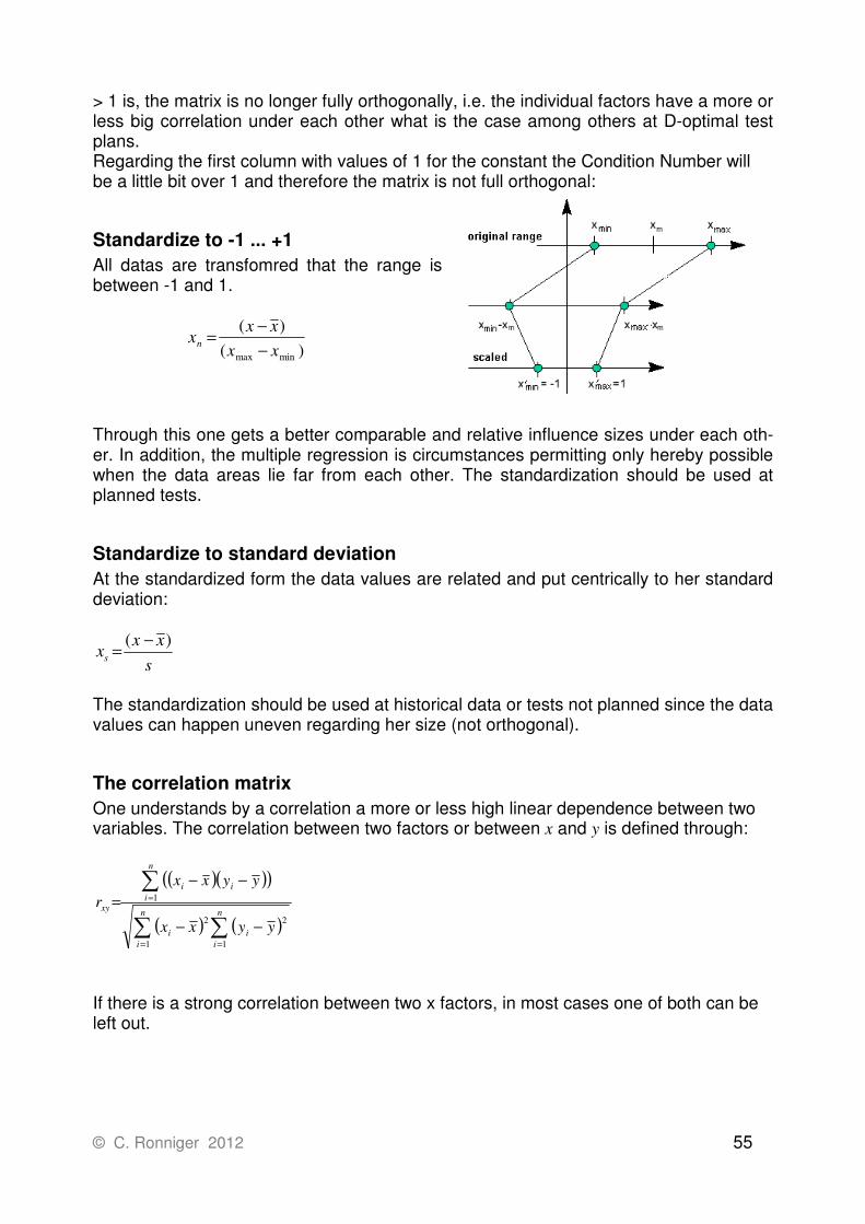
© C. Ronniger 2012 55
> 1 is, the matrix is no longer fully orthogonally, i.e. the individual factors have a more or less big correlation under each other what is the case among others at D-optimal test plans. Regarding the first column with values of 1 for the constant the Condition Number will be a little bit over 1 and therefore the matrix is not full orthogonal:
Standardize to -1 ... +1
All datas are transfomred that the range is between -1 and 1.
)(
)(
minmax xx
xxxn −
−=
Through this one gets a better comparable and relative influence sizes under each oth-er. In addition, the multiple regression is circumstances permitting only hereby possible when the data areas lie far from each other. The standardization should be used at planned tests.
Standardize to standard deviation
At the standardized form the data values are related and put centrically to her standard deviation:
s
xxxs
)( −=
The standardization should be used at historical data or tests not planned since the data values can happen uneven regarding her size (not orthogonal).
The correlation matrix
One understands by a correlation a more or less high linear dependence between two variables. The correlation between two factors or between x and y is defined through:
( )( )( )
( ) ( )∑ ∑
∑
= =
=
−−
−−=
n
i
n
i
ii
n
i
ii
xy
yyxx
yyxx
r
1 1
22
1
If there is a strong correlation between two x factors, in most cases one of both can be left out.

56 © C. Ronniger 2012
Response transformation (Box-Cox) For checking a possibly necessary response transformation the so called Box-Cox-transformation is used.
One after another the response is transformed according to the functions displayed be-low and the residues (SSr) are determined.
0)ln(
0)1(11
)( {=
≠−=
−−
λ
λλ λλλ
ifYY
ifYYY
The smaller the residues and therefore the deviations from the model to the measured data, the better is the transformation to be chosen. This has to be adjusted under the category data, as mentioned in the beginning. It must be pointed out that after the trans-formation single significances can be changed. Therefore on the side coefficients it has to be checked, if the model has to be corrected. The Box-Cox-transformation can just be executed, if a target factor-transformation has not yet been chosen.
λ-2 -1 0 1 2
ln(
Re
sid
ue
n )
-13.5
-13.0
-12.5
-12.0
-11.5
-11.0
1/Y² 1/Y 1/√Y ln(Y) √Y Y Y²

© C. Ronniger 2012 57
Transformation Inverse function Example for a’=1, b’=1 c’=0
1 ''' ' ceaY Yb +=
−=
'
''ln
'
1
a
cY
bY
2 ( ) '1'' ' ceaY Yb +−= −
−−=
'/)'(1
1ln
'
1
acYbY
3
+−=
1
'1''
'Yce
baY
−−
= 1'/'1
'ln
'
1
aY
b
cY
4 ( )''ln'' cYbaY +=
−=
''
1'
ceb
Y a
Y
5 )''('' cYbSinaY +=
−
= ''
'
'
1c
a
YArcSin
bY
6 ))''(1('' cYbSinaY ++=
−
−= '1
'
'
'
1c
a
YArcSin
bY
7 )''('' cYbTanaY +=
−
= ''
'
'
1c
a
YArcTan
bY
8
−=
Y
YY
1ln'
'1
1Y
eY
−+=
0 1 2 3 4 5
0
50
100
150
0 1 2 3 4 5
0.0
0.2
0.4
0.6
0.8
1.0
-4 -2 0 2 4
0.0
0.2
0.4
0.6
0.8
1.0
1 2 3 4 5
-8
-6
-4
-2
0
2
-1.5 -1.0 -0.5 0.0 0.5 1.0 1.5
-1.0
-0.5
0.0
0.5
1.0
-1.5 -1.0 -0.5 0.0 0.5 1.0 1.5
0.0
0.5
1.0
1.5
2.0
-1.5 -1.0 -0.5 0.0 0.5 1.0 1.5
-10
-5
0
5
10
0.2 0.4 0.6 0.8
-6
-4
-2
0
2
4
6

58
Statistical charts for One of the most important diagrams is the for the actual values of factors, marked by vertical red lines.
The respective adjustments can be changed by moving these red lines in the graphic with the mouse. By interactions also the other curve linearity’s are changed. The horzontal red line always shows the corresponding result value of the target factor. In addtion at indication of a lower or upper limit a blue horizontal line each does exist. The avantage of this depiction is that the math. model is visualized here directly and the gdients are a measure for influences. 15 curves in maximum can be depicted. Thereby the sequence in the list of independent factors under the category model is standard and can be changed there. The diagram Interaction-Chart
The diagram interactions resembles the curve diagram. The respective curses of curve are represented in pairs here. Every curve couple stands for the respective factors
© C. Ronniger 2012
harts for multiple regression
One of the most important diagrams is the Curve-diagram. Here all runs are for the actual values of factors, marked by vertical red lines.
The respective adjustments can be changed by moving these red lines in the graphic with the mouse. By interactions also the other curve linearity’s are changed. The hor
line always shows the corresponding result value of the target factor. In addtion at indication of a lower or upper limit a blue horizontal line each does exist. The avantage of this depiction is that the math. model is visualized here directly and the gdients are a measure for influences. 15 curves in maximum can be depicted. Thereby the sequence in the list of independent factors under the category model is standard
Chart resembles the curve diagram.
The diagram interactions resembles the curve diagram. The respective curses of curve are represented in pairs here. Every curve couple stands for the respective factors
© C. Ronniger 2012
. Here all runs are depicted
The respective adjustments can be changed by moving these red lines in the graphic with the mouse. By interactions also the other curve linearity’s are changed. The hori-
line always shows the corresponding result value of the target factor. In addi-tion at indication of a lower or upper limit a blue horizontal line each does exist. The ad-vantage of this depiction is that the math. model is visualized here directly and the gra-dients are a measure for influences. 15 curves in maximum can be depicted. Thereby the sequence in the list of independent factors under the category model is standard
The diagram interactions resembles the curve diagram. The respective curses of curve are represented in pairs here. Every curve couple stands for the respective factors

© C. Ronniger 2012
stands with his color with that one of these in an inbelow the scale). The factor StiffnRod has e.g. an interaction with DampRod. A line about StiffnRod with the identification (+) stands and one with the identification for the upper one (-) for the lower attitude of the over the colors. Interactions which aren't significant and taken out of the model aren't represented. So the complete connection is easily comprehensible in a look. The so called Effects, which are depicted in an own diathe top and lowest point of curves. Therefore they are dependent of the respectively actual factor adjustments. The effects are depicted as histogram sorted by their abslute size. Here you can recognize directly, where are the largest improvement potetials.
In the Pareto-chart all model terms are listed, whereas here the 95%present. Besides this the algebraic sign have been taken into account.Depending on the number of model terms, however the graphic can be complex (disavantage compared to the effect diagram).
stands with his color with that one of these in an interaction (see color of factor names below the scale). The factor StiffnRod has e.g. an interaction with DampRod. A line about StiffnRod with the identification (+) stands and one with the identification for the
) for the lower attitude of the factor DampRod. The assignment is possible over the colors. Interactions which aren't significant and taken out of the model aren't represented. So the complete connection is easily comprehensible in a look.
which are depicted in an own diagram, are respectively built from the top and lowest point of curves. Therefore they are dependent of the respectively actual factor adjustments. The effects are depicted as histogram sorted by their abs
can recognize directly, where are the largest improvement pote
all model terms are listed, whereas here the 95%present. Besides this the algebraic sign have been taken into account.
pending on the number of model terms, however the graphic can be complex (disavantage compared to the effect diagram).
59
teraction (see color of factor names below the scale). The factor StiffnRod has e.g. an interaction with DampRod. A line about StiffnRod with the identification (+) stands and one with the identification for the
factor DampRod. The assignment is possible over the colors. Interactions which aren't significant and taken out of the model aren't represented. So the complete connection is easily comprehensible in a look.
gram, are respectively built from the top and lowest point of curves. Therefore they are dependent of the respectively actual factor adjustments. The effects are depicted as histogram sorted by their abso-
can recognize directly, where are the largest improvement poten-
all model terms are listed, whereas here the 95%-scatter areas are present. Besides this the algebraic sign have been taken into account.
pending on the number of model terms, however the graphic can be complex (disad-

60
A further important graphic is the are displayed, where the respectively point is red instead of blue.
The better the model and the stability index, the more exact are the moobservations, resp. at the measure value. It would be ideal that all points would lie on the 45°-line. The deviations of every point of this line are called the method of the smallest error squares, the residues should be normal distributed acordingly. They can be depicted in a further diagram: Especially for depiction of influence of one or two factors to the response a Diagram can be chosen.
© C. Ronniger 2012
A further important graphic is the Model versus Observations, whereas here are displayed, where the respectively point is red instead of blue.
The better the model and the stability index, the more exact are the moobservations, resp. at the measure value. It would be ideal that all points would lie on
line. The deviations of every point of this line are called Residuesthe method of the smallest error squares, the residues should be normal distributed acordingly. They can be depicted in a further diagram:
for depiction of influence of one or two factors to the response a
© C. Ronniger 2012
, whereas here Outliers
The better the model and the stability index, the more exact are the model values at the observations, resp. at the measure value. It would be ideal that all points would lie on
Residues. Because of the method of the smallest error squares, the residues should be normal distributed ac-
for depiction of influence of one or two factors to the response a 2D or 3D-

© C. Ronniger 2012 61
It makes sense to use the factors, where an interaction exists. The diagram is created via the so called formula interpreter. Therefore the both variables (factors) are indicated shortened. The relative long formula over the diagram partly exists because of the re-conversion of standardization, on which the factors refer to. Those again you find in the tabular overview at the beginning. Alternative the diagram type can also be another one, e.g. level-curve diagram. This corresponds to the 3D-view above. The diagram type is selected under the menu point of the main window Dia-gram/Diagram-type. After this diagram selection there is no longer an internal refer-ence to the multiple regression. The diagram is seen as independent and is not actual-ized at modification of factors and so on.
Regulation of outliers
For the regulation of outliers one looks at the residua of the respective points, i.e. the deviations of the observations (measurements) to the model values. When this devia-tion is regarded as a outlier the test after Grubbs is recommended. The hypothesis is: xr is an outlier. xr stands for the values of the residua, sr for the standard deviation of the residua
α−− >= 1;
,
n
r
irr
i Ts
xxT
Tn,1-α is the critical worth of the Grubbs-Test after the following table:
n Tn,0,95 Tn,0,99
3 1,15 1,16 4 1,46 1,49 5 1,67 1,75 6 1,82 1,94 7 1.94 2,10 8 2,03 2,22 9 2,11 2,32
10 2,18 2,41 12 2,29 2,55 15 2,41 2,71 20 2,56 2,88 30 2,75 3,10 40 2,87 3,24 50 2,96 3,34
100 3,21 3,60

62 © C. Ronniger 2012
Optimization
One understands by an optimization of regression models finding the right adjustings of all factors for a minima, maxima or a predefined set point of the response variable.
Example: For the model Y= 1 + 2⋅A + 3⋅B + 4⋅C + 5⋅D +6⋅A⋅B the minimum should be found.
The attitudes of -1 are obviously the best points for all factors. Y has the value-7. Due to the interaction the considerably better minimum is the result, however with Y= -15 by 1;-1;-1;-1
At the search for the best point all mutual attitudes must be checked because of a pos-sible turning back of the gradients. At the search for an optimal attitude for several response values a conflict can be ap-pear if the best points lie in an opposite direction. A compromise must be found here. One works for it with a so-called fulfilment degree which yields a summarized value for all response values. The result is the corresponding "wish function". At first a plausible
-1 0 1 -1 0 1 -1 0 1 -1 0 1
Y
-4
-2
0
2
4
6
A B C D
00 00 00 00
Y = 1 +/- 7,18E-19Y = 1 +/- 7,18E-19
-1 0 1 -1 0 1 -1 0 1 -1 0 1
Y
-15
-10
-5
0
5
A B C D
11 -1-1 -1-1 -1-1
Y = -15 +/- 2,15E-18Y = -15 +/- 2,15E-18

© C. Ronniger 2012 63
significant model is determined and an optimum of each model is found. It can already happen that some factors are not significant for all response variables. After that the
optimization of all repsonses is together carried out via the degree of performanceη:
( )∑=
−
−= ⋅
m
i ii
jii
iMinMax
YOpt
1
,
2
δη
with m = Number of response variables max/min = the respectively greatest and smallest Y value Yi,j = current model response for every response value at the continuous variation steps j
δ i = weighting factor for every response variable
If certain response values have maybe a higher importance than other, this can be taken into account by a weighting factor δ.

64 © C. Ronniger 2012
Discrete Regression
The Multiple Regression requires steady target values. However, it also can happen that the target value has qualitative character or only 2 expressions (e.g. component has a rip or is i.O). One usually uses the so-called Discrete Regression for this way of the evalua-tion. The coefficient of the model is carried out the determination via the Maximum Like-lihood-Method. This is in the equal dialogue window as the multiple regression treats. There are some unusual features and restrictions, though. The result describes the probability that the target value takes a certain expression. Therefore it is to fix data in addition to which this probability applies (here expression 1) in the category. Being the so-called pseudo-R² indicated instead of the certainty measure R² in the cate-gory of regression. LL consists this of the lying Likelihoods, short. Another indicator is the deviation D= -2 LL. Since in the discrete regression probabilities are treated here does not exist any residua respectively the Sum of Squares. So instead of the ANOVA a combination of the identification values is represented. For this reason the choice of the graphics does not contain any diagram types which represent residua either. The Box Cox transformation is not here necessary because the transformation of the target value is already provided tightly on "Logits". The curve diagram contains typical S curves, because for the discrete regression probabilities under 0 and over 1 are not possible.
An special feature of the logistical regression is the evaluation of the groupings. The factors are . groups summarized here in classes. The number of response value ex-pressions is counted (H event). One divides this number by the group quantity (H ob-servations), one gets the observation probability (P observations), the probabilities found out with these from the model (P expected) compared and tested against a critical
χ-value.
Discrete regression bases One understands an evaluation by a discrete regression with target values which do not have any steady measurement but qualitative character. The result of an examination could be judged only "well" or "badly", as rip available or not, for example. These state-ments represent the undermost level of the determinable. It should always be aim to receive the "dissolution" as best as possible, i.e. at least one graduation like a beginning
2000 3200 4400 0 0.5 1
Pro
ba
bili
ty f
or
Y=
Ye
s
0.0
0.2
0.4
0.6
0.8
1.0
x2 x3
32003200 0.50.5
0.76380.7638

© C. Ronniger 2012 65
rip, rip by centre, rip almost complete and ragged. The evaluation with the standard mul-tiple regression is still possible. The graduation has to be defined with as equal dis-tances as possible. Furthermore if only 2 expressions are possible (bad/good or black/white) the following procedure can be applied. For example the data is given:
this one for the not satisfactory following regression leads (straight line approximation):
It makes more sense to represent the probabilities here instead of the direct representa-tion of the target value that a "condition" enters. One almost combines x areas to come "onto countable events" to this (classification). The table then becomes:
The x values are assigned to the groups of 1, 2 and 3 (according to a centric classifica-tion, here on integer numbers). The number is y = 1 counted (how it is "good" and "bad" at concepts to fix on what counting refers e.g. open "badly") within these groups now. From this the relative frequencies can be calculated per group. If one represents these, then a substantially better relation arises:
y 0.01791835 0.24306638 x·+= r = 0.459
X
0.5 1.0 1.5 2.0 2.5 3.0
Dis
cre
te R
es
po
ns
e
0.0
0.5
1.0

66 © C. Ronniger 2012
This is bought by a diminution of the x information, i.e. for this evaluation considerably more observations are used than at steady measurands. Originally this one makes 12 informations in the previous example stand, 3 at the disposal only what is a correspond-ing disadvantage. Under circumstances too few degrees of freedom are entitled at the evaluation for the regulation of possible interactions at the disposal. Since it is pure ob-servations here but usually (not around planned tests), however, sufficient data are as a rule also available. Estimators are the formation of the relative frequencies for the probability P simultane-ously, it becomes y =1. It is valid:
group
i
in
np =
ni = number of y=1 (can not be 0, usually ngroupe >= 5) For ni < 0 and ni > 4 nonsensical probabilities of P < 0 and P > 1 give up, though. There-fore suitable transformations are necessary. A transformation frequently used for this problem definition is the so-called Logit model:
−=
p
py
1ln'
respectively
−=++
p
pxbxbb zzo
1ln.....11
The expression P/(1-P) represents odds and the meaning has admission probabil-ity/counter-probability. One also speaks here about Logits. A little strange, it is the deal-ing with odds and the interpretation one is horse bets, then, because the odds corre-spond to the quotas here. It is important to notice that the logistical regression treats not probabilities but probability conditions.
y 0 0.25 x·+= r = 1.000
X
0 1 2 3 4
Re
lati
ve
Fre
qu
en
cy
fo
r Y
=1
0.0
0.5
1.0

© C. Ronniger 2012 67
To remove the low limit of the domain in addition, the odds become in addition logarith-miert. The inverse function is needed for the inverse function after the regulation of the model parameters on probabilities also here:
ye
pˆ
1
1ˆ
−+=
This also is described as a "logistical" distribution function. The limits P = 0 and P = 1 about the Logit are not portrayable. The number ni per group should not be 0 anyway. With steady target values the prerequisite for the method of the smallest error squares for the estimate of the sought-after coefficients b is that the error deviations have an identical variance at the regression. This is not the case here. Therefore a weighted re-gression must be used. To this an estimator is needed for the variance. The already established relation became a determination of the coefficients at not weighted regres-sion till now
( ) YXXXBTT 1ˆ −
=
used. At the logistical regression there is the problem that the variances of the model errors are not constant. Through this the variances of the model estimators cannot be minimised about the method of the smallest error squares. However, the problem can be removed by a weighted regression. Be the variances of every observation needed to this, these through
)ˆ1(ˆˆ 2
iii pps −=
you define. The estimators for the regression coefficients then determine themselves through:
( ) 'ˆ 1YXXXB
TT δδ−
= with
).......,,(22
2
2
1 nsssdiag=δ
Y ' is the vector of the corresponding Logits. A new problem arises, however. The esti-mators determine itself only from the result of the calculation. So an iterative calculation must be carried out. Another possibility for the regulation of the model parameters is the maximum Likeli-hood, short ml method. The basic concept is relatively simple. The parameters are cho-sen so that the valued variables are the most similar to the observations in the data set (Likelihood). The similarity is, described by the so-called Likelihood function this one the Likelihoods of all cases of the data set consists of the product:
∏=
−−⋅=n
i
iiiyiy
ppLH1
1)ˆ1(ˆ
Yi dates from the n observations, ip

68 © C. Ronniger 2012
from the model. The coefficients of the model are to search so now that LH gets maxi-mum. It is like a probability, can accept a value between 0 and 1 since a little similar to the likelihood of a single case. Likelihood the product of many numbers between 0 and 1 gets minute, though, therefore becomes also here LH is logarithmized and is made it this LL lied short:
∑=
−⋅−+⋅==n
i
iiii pypyLLLH1
)ˆ1ln()1()ˆln()ln(
There is no analytical solution for the two variants. The coefficients also must be deter-mined iteratively in which at first one chooses an arbitrary start value. With these the
Logits and the first estimated values of the probabilities ip can being certainly. The
product of the LH function or the sum is charged to the LL with that for every data se-ries. The same must repeated as long, as no greater LL-value can be found It is the most important advantage of the maximum likelihood method, that for the regu-lation of the coefficients no group formation of the data is required (can contain 0 events, where Logits are not calculable). A dimension for the quality of the found solution is the deviation:
LLD 2−= The omen is changed since the logarithmic value between 0 and 1 is always negative.
One gets in addition one (χ²-distributed value which means how badly the model de-scribes the data through this with the factor 2. Therefore it is all the better the smaller this value is. At the normal multiple regression the certainty measure R² is primarily indicated for the quality of the model. There is no direct correspondence, however, a pseudo-R² was de-fined by McFadden:
0
1
0
102 1LL
LL
LL
LLLLR MF −=
−=
LLo : Log-Likelihood of the model, this is only the constant y ' = bo LL1 : Log-Likelihood of the concrete model y ' = bo+ b1x1 + can not reach the value 1, as a rule, values from 0,2 to 0,4 are already regarded as a good model customization. For the assessment of the significance of the individual coefficients (factors) the devia-tion test is recommended. It is checked whether the model shows with the respective factor compared with this without just this significant difference. For the check of a factor the difference of the deviation is formed:
( )FFF LLLLLLLLD −−=−−−=∆ 11 2)2(2 in which the index F stands for the model without the factor to be looked at compared with the exit model with the index 1 (see pseudo R²).
With the χ²-distribution as well and the degrees of freedom df = 1, the p-Value = 1 - α can be determined.

© C. Ronniger 2012 69
The complete model also can analogously be tested (see pseudo R ² in turn) compared with the "zero model" to this. The Differenzdevianz is:
( )012 LLLLDG −−=∆
df = with the degree of freedom: z = number of factors, interactions etc.. Relatively to the power of computation effort means one this approach, however, be-cause the ml iteration must be carried out for every factor to be checked. As an alterna-tive to it the woods test frequently mentioned can be used. This is like the t test at the normal regression. The test quantity is for every factor:
2
,
2
=
jb
j
js
bχ
with
*
,, jjjb Xs =
and
( ) 1* −= XXX
Tδ the already established diagonal matrix was and in which (from the variances of every observation series.

70 © C. Ronniger 2012
5. Multivariate Analises
Cluster Analysis One understands essentially a grouping of unordered data (e.g. measurements, image dots etc.) by a cluster analysis. For example:
The grouping is made by similarity characteristic. As a rule, these are distance data as the represented picture shows. In this case there is a high similarity if the data points have a distance as low as possible to each other. d = degree of heterogeneous = measures for the assessment of the distances between the objects
Euklid’s distance :
( ) ( )2
12
2
12 yyxxd −+−=
City-block Distance :
1212 yyxxd −+−=
Tschebyscheff distance :
( )1212 ;max yyxxd −−=
Y
X
2
1 Euk
City
Tsc
There can exist similarities also in form of a correlation matrix. The higher the correla-tion is, the more similar the "objects" are to each other. So a greater value is relevant here. There doesn't exist the initial data in the form of coordinates but there is a matrix where is shown a relation from each object to each other. The measurement to this is described by the correlation coefficient r. In this case the object distance is d=1-r be-cause the objects more nearly, the higher the correlation is. As an alternative to this of-ten d=ArcCos (r) is used. Respectively higher distances caused through this equation. The similarities can not be related by data in rows but with the titles and the data col-umns. Therefore here has to be created first a correlation matrix before the cluster anal-ysis.
Y
XX
Group 1
Group 2

© C. Ronniger 2012 71
The targets of building clusters are:
- Creating a simplified more open structure - Data reduction - Recognizing of connections
In Visual-XSel there is implemented the hierarchical agglomerative method. The advantages are:
- No specification regarding number of clusters necessary - Additional reduction of the clusters by "limit distance" possible - Every run yields the same result - Efficient algorithm to be implemented easily - Graphic representation option of the clusters as a tree structure
The method shall be clarified at a simple example. The following objects are given with their coordinates:
Only 2 coordinates are represented here. n dimensional coordinates (columns) are possible where 3 coordinates can be visualized in a 3D-diagram. The distance matrix arises from the coordinates. (Values = Euklid’s distances):
The first cluster (object pair) is carried out via the smallest distance. This is between B and D with the distance of 1.4. Between this points there will be created a new center with the name BD.
x y
A 9 4
B 0 4
C 7 9
D 1 5
E 8 1
F 10 0
G 11 10
A B C D E F G
A 9,0 5,4 8,1 3,2 4,1 6,3
B 9,0 8,6 1,4 8,5 10,8 12,5
C 5,4 8,6 7,2 8,1 9,5 4,1
D 8,1 1,4 7,2 8,1 10,3 11,2
E 3,2 8,5 8,1 8,1 2,2 9,5
F 4,1 10,8 9,5 10,3 2,2 10,0
G 6,3 12,5 4,1 11,2 9,5 10,0

72 © C. Ronniger 2012
The coordinates of the new group are calculated by XBD = 1/2 (XB+XD). YBD = 1/2 (YB+YD). Correspondingly applies to the next group XAEF = 1/3 (XA+XE+ XF)… If there exists, how-ever, only a distance matrix, then the cluster centre can be determined also about the following geometric relation:
( )2
2 222
EFAFAE dbdd
−+⋅=
The results of both variants, however, do not yield exactly the same because the geo-metric center is calculated is here only a approximation method. The distance of E and F amounts to 2.2 and therefore represents the 2nd group. The 3rd group is already a combination of 3 points AEF. After every run the complete table must be built up newly. At the first summary the partner B will be deleted (values in column and line). Instead of D it will be set BD with the new distances to the remaining objects calculated with the given formula (bold values). It's better to define here BD and not DB
The table goes down always further until 2 partners are only left. The individual steps can be clarified as a tree structure, also called dendrogram The distances of the groups get longer from left to right. At the end of this algorithm, the last group will include all combinations. Instead of the dendrogram one can have a structure list
A B C BD E F G
A 5,4 8,1 3,2 4,1 6,3
B
C 5,4 7,2 8,1 9,5 4,1
BD 8,1 7,2 8,1 10,3 11,2
E 3,2 8,1 8,1 2,2 9,5
F 4,1 9,5 10,3 2,2 10,1
G 6,3 4,1 11,2 9,5 10,1
G
C
F
E
A
D
B
4,1
2,2
1,4
3,51
7,27
8,61

© C. Ronniger 2012 73
Through direct specification or definition of the distance a desired number of clusters can be achieved. The last two summaries are not carried out. Categorial characteristics can not be defined directly. It is necessary to transform the basis data in a numerical format first. This can be done by producing columns with worth of 1 and 0 to describe the expressions. For example y can be transformed into the following numeric format:
Basis data New structure
x y x ya yb yc
A 9 a A 9 1 0 0
B 0 b B 0 0 1 0
C 7 c C 7 0 0 1
D 1 a D 1 1 0 0
E 8 b E 8 0 1 0
F 10 c F 10 0 0 1
G 11 a G 11 1 0 0
G
C
F
E
A
D
B4
3,51
G
C
F
E
A
D
B3
7,27
G
C
F
E
A
D
B2

74 © C. Ronniger 2012
Principal Component Analysis PCA The Principle Component Analysis calculates new so-called latent variables. These are shortened called factors and represent the Principle Components PC. Do not mix up this name with the factors by DoE. It is the target to describe all existing variables with few factors (data reduction). With the variables x1 and x2 and its measurement points the principle shall be described like shown on in the following picture.
The measurement points lie in an ellipse which location depends on the correlation be-tween the variables. A new axis system arises by moving the zero point and turning the coordinate system. The first so-called main axle rejects in the direction of the greatest spread of the standardized values of x1 and x2. The second main axle stands vertically on the first one and explains the lower share of the variance. Therefore one also de-scribes the principle components as eigenvectors. For the determination of the principle components so-called factor loadings P and Score values T are defined. The factor loadings describe the situation of the PC to the original coordinate system of x1 and x2. The dimension of the factor loadings is -> number of components x number of variable x. The Score values T describe the projections on the main axles for every point. The dimension of T is -> number of component x number of measurements. The connection is in matrix notation:
TPTX =
The following condition applies to the factor loadings:
1...22
2
2
1 =++ kppp
The Principle Components are calculated through the Score-values ti and the eigenva-
lues λi :
i
ii
tPC
λ=
The eigenvalue λi describes, how much of the total spread of all variables is declared through the factors. The eigenvalues also serve for the decision whether factors in the model can be kept or left out. If the eigenvalue is less or equal 1, it explains less or equal of the variance of one variable. If this is the case the factor can be left out. eigen-values and eigenvectors yield an independent structure of each other (orthogonal).
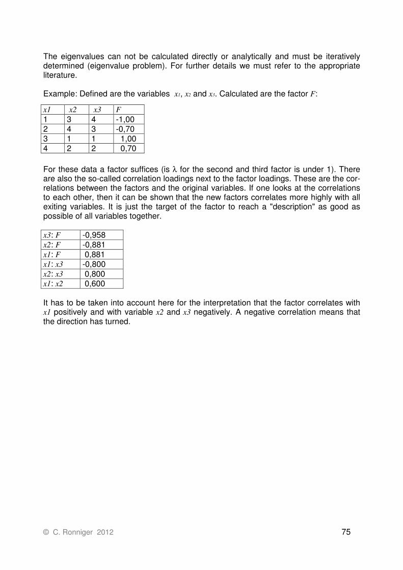
© C. Ronniger 2012 75
The eigenvalues can not be calculated directly or analytically and must be iteratively determined (eigenvalue problem). For further details we must refer to the appropriate literature. Example: Defined are the variables x1, x2 and x3. Calculated are the factor F:
For these data a factor suffices (is λ for the second and third factor is under 1). There are also the so-called correlation loadings next to the factor loadings. These are the cor-relations between the factors and the original variables. If one looks at the correlations to each other, then it can be shown that the new factors correlates more highly with all exiting variables. It is just the target of the factor to reach a "description" as good as possible of all variables together. x3: F -0,958 x2: F -0,881 x1: F 0,881 x1: x3 -0,800 x2: x3 0,800 x1: x2 0,600 It has to be taken into account here for the interpretation that the factor correlates with
x1 positively and with variable x2 and x3 negatively. A negative correlation means that the direction has turned.
x1 x2 x3 F
1 3 4 -1,00 2 4 3 -0,70 3 1 1 1,00 4 2 2 0,70

76 © C. Ronniger 2012
Partial Least Square (PLS) PLS was developed 1960 of the Swedish econometrist Herman Wold. PLS means: Par-tial Least Squares Modeling " into latent variable " . The purpose is primarily the evalua-tion of correlating data or the evaluation of mixture plans, where the standard method Multiple Linear Regression (MLR) isn’t practicable. It is also an essential advantage of PLS that much variables can be processed. It is even possible to evaluate with less in-formation (data rows) than variables exist. This is not possible with MLR. The represented picture shows two variables x1 and x2. The main component analysis PCA with tPCA lies in the "bump" of the ellipse. The greater x1 and x2 correlate, the longer tPCA gets. If there is no correlation, the vector direction is not defined by tPCA any more, because the ellipse then becomes a circle and has no more preferred direction.
The component of tPLS however is then still determinable about the analysis of the co-variance. This is a decisive advantage of PLS over PCA. The results, i.e. the coeffi-cients of the variables, are then identical with the MLR method (for orthogonal data). While the MLR method provides no longer clear results or completely gets out at very correlating data, furthermore the PLS method can be used. Even if two variables have a correlation or 100%, this is still possible. Of course the assignment of the effects is then no longer clear, in this case PLS shares the effects half to the two variables. It is the disadvantage of the PLS method that the forecasts and R² are worse than at MLR. The coefficients are partly also fundamentally smaller, what causes to estimate the effects too little.
PLS is very related with PCA. Instead of the loadings (PCA) here is the weight matrix W relevant
TWTX =
T are the so-called Scores of the components. W includes the response y, which doesn’t exists in PCA. Also here the following condition applies to the weights:
1...22
2
2
1 =++ kwww
The regression model is defined with:
TcTy =ˆ
where c is the regression coefficient.
x2
x1
Y
t PCA
t PLS t MLR
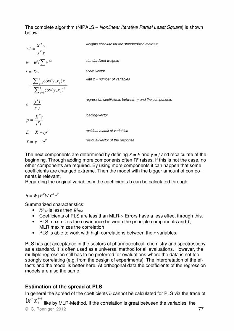
© C. Ronniger 2012 77
The complete algorithm (NIPALS – Nonlinear Iterative Partial Least Square) is shown below:
yy
yXw
T
T
=' weights absolute for the standardized matrix X
∑= 2'/' www standardized weights
Xwt =
∑
∑
=
==z
j j
z
j jj
xy
xxy
1
2
1
),cov(
),cov(
score vector with z = number of variables
tt
tyc
T
T
=
regression coefficients between y and the components
tt
tXp
T
T
=
loading-vector
TtpXE −= residual-matrix of variables
Ttcyf −= residual-vector of the response
The next components are determined by defining X = E and y = f and recalculate at the beginning. Through adding more components often R² raises. If this is not the case, no other components are required. By using more components it can happen that some coefficients are changed extreme. Then the model with the bigger amount of compo-nents is relevant. Regarding the original variables x the coefficients b can be calculated through:
TT cWPWb 1)( −=
Summarized characteristics:
• R²PLS is less then R²MLR
• Coefficients of PLS are less than MLR-> Errors have a less effect through this.
• PLS maximizes the covariance between the principle components and Y, MLR maximizes the correlation
• PLS is able to work with high correlations between the x variables.
PLS has got acceptance in the sectors of pharmaceutical, chemistry and spectroscopy as a standard. It is often used as a universal method for all evaluations. However, the multiple regression still has to be preferred for evaluations where the data is not too strongly correlating (e.g. from the design of experiments). The interpretation of the ef-fects and the model is better here. At orthogonal data the coefficients of the regression models are also the same.
Estimation of the spread at PLS
In general the spread of the coefficients b cannot be calculated for PLS via the trace of
( ) 1−XX
T
like by MLR-Method. If the correlation is great between the variables, the

78 © C. Ronniger 2012
spread can be estimated only via a so-called cross validation. The disadvantage here is a not definite result and the calculation needs much computing time. To calculate and applicate here the p-Value, like at MLR is not recommended here. For PLS and the variable selection there is much better suitable the so-called VIP-indicator
Variable selection with VIP
For using the PLS-Method and the variable selection here it is suitable to consider the VIP-indicator. VIP is an abbreviation of Variable Importance in the Projection. That means how much is the influence of the variable in the projection of the scores t. This indicator is first launched by Wold in 1993. VIP is calculated for each xj via:
∑∑==
=
h
k k
T
k
k
Th
k
jk
k
T
k
k
T
jtt
tyw
tt
tyzVIP
11
2
with h = number of components, z = number of variables x (e.g. terms)
The y-vector must be standardized first. In the literature there is described a limit for VIP between 0,8 …1. A too less value indicates, that the variable can be left out. But expe-riences has shown, that VIP<0.5 are not unusual for important variables If there is the question whether a variable should be left out from the model, the coeffi-cient size also has to be taken into account. Also the technical connections should be considered. PLS charts Especially for evaluation of PLS-Analysis there are two important charts, the Score Plot and the Correlation Loading Plot. These charts can be selected under the rubric charts (after PLS data analysis via menu Statistics of the spreadsheet). Score Plot The Score plot represents every measurement point about the most important Scores t1 and t2. Possible samples and characteristics in common can be recognized. Also out-liers can be recognized.

© C. Ronniger 2012 79
Correlation Loading Plot In the so-called Correlation Loading Plot the professed variances of the variables and the target value are represented indirectly on the components PC here. The axis are scaled as correlations, so it is: professed variance = correlation^2. Hereby the influences of the variables are shown and one recognizes which compo-nents describe the variables better. The ellipses describe 100% (outer) and 50% (inner) professed variance
The nearer the variables are to the 100% ellipse, the more important these are. In this example the component PC1 describes the variables x1, x2 and also the response y approximately alone, while the variable x3 needs both components.
PC1
-1.0 -0.5 0.0 0.5 1.0
PC
2
-1.0
-0.5
0.0
0.5
1.0
X3
X1
X2
Y

80 © C. Ronniger 2012
6. Neural Networks The fascination starting out from neural nets consists that they are able to solve prob-lems of high complexity with simple means in some cases. The nerve cell represented in simplified terms the biological equivalent. (one guesses that about 100 billion neurons or nerve cells are responsible for the information processing and storage in the brain). It is necessary in regard on a problem definition to be examined for neural nets neither to carry out more exact examinations nor to represent a formal model explicitly. No ef-fortful algorithms are needed, there is merely the task to approximate data. Doesn't pass any guarantee for the training success either and the solutions can be different, though. Depending on number of neurons the NN almost exclusively represents interactions. In principle nonlinear connections can be included. It is the advantage of the NN to be able to produce almost arbitrary curses of curve with several maxima and minima primarily while the relatively simple polynomials of the multiple regression can show at most cu-bic functions. NN is therefore also often used where e.g. characteristic maps shall be calculated by engines. A found model only applies to the current attitude of the respectively other factors. Influ-ence on the curses of curve of the others has a change of one or several factors in the high measure. One knows this behavior at the multiple regression also in connection with interactions, this is sometimes confusable. It is therefore more difficult to declare connections here.
Topology Example with 3 Factors
The so-called neuron has essentially an assignment or activation function. This is the math-function tanh in most cases. The output of the neuron is between -1 and 1.

© C. Ronniger 2012 81
With the weights W the quantitative effect of the neuron is fixed. On the initial side every neuron of every factor has also weighted entrances as well as in addition a constant value C over cross. The general model is:
∑ ∑= =
++=
k
j
z
i
jiijjo wxcWCY1 1
,tanh 1
1tanh
2
2
+
−=
x
x
e
e
k = number of neurons z = number of factors In principle, the factors xi are standardized between-1 and +1
Number of parameters = z⋅ k+ k⋅ 2+ 1
The output of the represented neurons can be inputs of wider neurons again. One calls this layered nets which shall not be given further treatment here. The number of neurons doesn't have always to be so large like that one of the factors. Besides arbitrary further combinations the following representations are possible: z < k
x1
Σ Y
W⋅ 1
W⋅ 2
W⋅ 3
x2
ye
2 x·1-
e2 x·
1+
=ye
2 x·1-
e2 x·
1+
=
ye
2 x·1-
e2 x·
1+
=ye
2 x·1-
e2 x·
1+
=
ye
2 x·1-
e2 x·
1+
=
ye2 x·
1-
e2 x·
1+
=
x
-4 -2 0 2 4
Ou
tpu
t
-1.0
-0.5
0.0
0.5
1.0

82 © C. Ronniger 2012
z > k
x1
Σ Y
W⋅ 1
W⋅ 2
x2
ye
2 x·1-
e2 x·
1+
=ye
2 x·1-
e2 x·
1+
=
ye
2 x·1-
e2 x· 1+
=
x3
As a rule, a higher number of neurons as factors has, however, the disadvantage of the over-fit. The results can get relative discontinuous The most suitable model is dependent on the facts and can't be generalized. Besides the activation function tanh one also finds the following functions: Function Name
Y’ = x’ Linear
Y’ = sign(x’)
Signum
Y’ = tanh(x’)
Sigmoid
2)'2/1(
'x
eY−=
Normal-distribution
Exactly as in the case of the multiple regression there is to consider knowledge about the facts, which are to be examined. The corresponding activation function also has to be used for purely linear connections. E.g. the signum-function has to be chosen for switching processes or digital statements.
Training-Algorithm Unlike the multiple regression a clear analytical solution isn't possible by means of ma-trices here. The coefficients or weights are determined by a training algorithm rather iteratively. Meaningful start values for the training are:
wi,j : ±5
cj : ±2
Wj : ±(Ymax -Ymin)/2

© C. Ronniger 2012 83
Co : (Ymax+Ymin)/2 (is fix) There often are several roughly equal solutions to the approximation of the available connections. However, there is a high risk to find only a local optimum. The model pa-rameters, as in the case of the multiple regression, are sought. Instead of the polynomi-al coefficients the parameters the so-called model weights and the constants are here. The training process aims minimize the square sums between NN model and data (leases square method) and is nothing else but an optimization method. These are de-scribed in detail in the literature. Methods which take into account the gradient of the object function for the search for the optimum are judged particularly well. It is a general problem that the training algorithm doesn't stop in a local minimum but searches the complete parameter room for the global minimum. The following picture shows the dev-iations for two parameters (weights) for the training data. This is necessary to minimize. Depending on start condition, perhaps a local minimum is found and this suggested as the solution. If there are no further investigations to search for other minima, not the best one will be found.
Depending on number of neurons the computation effort can increase considerably. A complete variation of all parameters is no longer feasible as of a certain number of fac-tors and neurons. To prevent that one finds only a local minimum, several different "start points" are used for the weights at the training. To this several start points must be selected in sufficiently large number by randomizer. After an abort condition to be fixed the next optimization step is calculated with the weights of the best customization. These optimizes the best point adjusts iteratively for every weight. It happens, that in the practice there are much more or less equal solutions. I.e. the approximation to the data on hand many local minima in the range can be reached well by completely different weights equally (the global minimum).
Neural Network as an alternative for multiple regression In principle, the neural network of the multiple regression is different by the networking and particularly by the activation function. One chooses the linear activation function for this then we will get the same as a polynomial of the regression:

84 © C. Ronniger 2012
The represented example of 3 factors corresponds to the model C = 0 and W = 1:
Y = x1⋅w1 + x2⋅w2 + x3⋅w3 + Co
c and W having to be set in the definition of the start weights, so that they aren't further varied. Interactions and square terms can be formed by pseudo-factors (e.g. x4 = x1 × x2 etc.).
The training of this simple network must cause the equal clear result of the multiple re-gression. The weights then correspond to the coefficients. It would be the advantage of this procedure, for example, that certain coefficients are already known and become as "extremely" respected for technical or physical reasons. One then sets these values for the start weights as fix, and only looks for the remaining coefficients (weights). This isn't possible with the multiple regression.
Attributes of Neural Networks • A Neural Network is a dynamic system which is able y = f (x) execute, an arbi-
trary function.
• The structure of a Neural Networks is defined by the number of elements, by the special topology and by the way of the activation function.
• One doesn't program a Neural Network but one trains it. Instead of a rule or a general algorithm the training demands a certain number of data.
• The "knowledge" of a Neural Network (longtime memory, program) sits in the to-tality and in the activation threshold of the elements. No clear symbolic form has this knowledge but a chaining is of factors, constants and weights whose connec-tion cannot simply be recognized in comparison with the model of a multiple re-gression.
• There isn't any difference between hardware and software in the Neural Net-works: It can be considered independent machines or has been simulated via software as a model.

© C. Ronniger 2012 85
Example For example in an engine control the following characteristic map for an inlet spread of a camshaft. The parameters are filling and speed:
The normal regression cannot represent this even with a cubic model. The Neural Net-works which offers more "degrees of freedom" to the approximation offers its services here. Due to the many discontinuities it will be necessarily to use a higher number of neurons as parameters. 10 neurons were used for the customization represented be-low:
Fill
10
20
30
40
°
Sp
rea
d
60
70
80
90
100
110
120
1/ min
Speed
1000
2000
3000
4000
6000
Fill
10
20
30
40
Sp
rea
d
50
60
70
80
90
100
110
120
Speed
1000
2000
3000
4000
5000

86 © C. Ronniger 2012
Further statistical charts
Scatter bars In practice it frequently occurs that certain circumstances are illustrated with just one or a few measurements. If you ascertain that the result scatters more or less, in most in-stances the median is built. This is absolutely permitted, if the value staggers marginally after repeated measurements. But if there are larger variations, different test series are difficult to compare to each other, especially, if outliers do occur. Possibly you will get no unique compromise output. An illustration with Scatter bars will help in this case. Here an example:
In 4 test series the values respectively listed among each other have been quantified. After selection of the menu point Statistic/Scatter bars the following diagram results:
Please note that the titles of columns (legend) standing in the first row are used as X-axis title. The first column is also used as series and is not interpreted as reference to the x-axis like at the most other diagram types. If the median and the Scatter s is just known from samples (resp. measurements) and a predication should be made about the totality (then infinitely many measurements should be executed), so a so called confidence belt can be indicated, in which the true median lies with PA % probability. If you choose maximal and minimal value in the dialog window Statistics/Scatter bars, just the maximal and minimal value of the entered data (sample) will be determined, as shown here in the example. If the number of samples would be increased, so another maximal or minimal value could be found. For this reason it is recommended to choose one of the 3 confidence belts, which are available. Particularly here the outliers do affect not so seriously. Activate the menu point Options/Show data, to type out the medians and the confidence belts resp. the min/max-areas in the diagram. Those are also in the graphical data (ta-ble menu point Insert/Graphic-data).
A
90
50
70
40
B
100
64
75
52
C
110
52
72
50
D
104
65
84
48
8 B C D
0
20
40
60
80
100
120

© C. Ronniger 2012 87
Boxplot The boxplot is a special type of frequency scale. Here the values are depicted via the y-axis instead of the x-axis, whereas several boxplots in parallel are possible in one dia-gram. In the middle of the boxplot there is a line with the so called center-value resp. median. Optional also the median can be chosen. Within the inner field there are 50% of all values. Within the outer margin lines top and down are 99% of all values. Optional also the smallest and largest occurring value can be displayed (min/max-values). If there are too little data values, the 99% areas correspond to those of the min/max-values. In opposite to the frequency scale with Gauss curve here you get a rapid comparison about the respective status of several series. The values of the respective series are written among each other. In the first row there is the reference to the X-axis resp. the legend for the single boxplots. An example for following table values:
After selection of diagram type boxplot vertical the following develops:
Optional the single values can be depicted as eye-catcher-points with their numerical values. See also Boxplot horizontal, Scatter bars
A
3
6
7
7
8
B
5
7
8
9
10
C
4
6
7
8
9
A B C
0
2
4
6
8
1 0
1 2
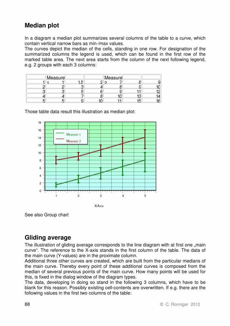
88 © C. Ronniger 2012
Median plot In a diagram a median plot summarizes several columns of the table to a curve, which contain vertical narrow bars as min-/max values. The curves depict the median of the cells, standing in one row. For designation of the summarized columns the legend is used, which can be found in the first row of the marked table area. The next area starts from the column of the next following legend, e.g. 2 groups with each 3 columns:
Those table data result this illustration as median plot:
See also Group chart
Gliding average The illustration of gliding average corresponds to the line diagram with at first one „main curve“. The reference to the X-axis stands in the first column of the table. The data of the main curve (Y-values) are in the proximate column. Additional three other curves are created, which are built from the particular medians of the main curve. Thereby every point of these additional curves is composed from the median of several previous points of the main curve. How many points will be used for this, is fixed in the dialog window of the diagram types. The data, developing in doing so stand in the following 3 columns, which have to be blank for this reason. Possibly existing cell-contents are overwritten. If e.g. there are the following values in the first two columns of the table:
X - A xis
1 2 3 4 5 0
2
4
6
8
1 0
1 2
1 4
1 6
1 8
M easure 1
Measure 2
12345
Measure 1
12345
1,5
3579
2468
10
Measure 2
789
1011
89
111315
9
10121416

© C. Ronniger 2012 89
1 . 1 . 2 0 0 0
2 . 1 . 2 0 0 0
3 . 1 . 2 0 0 0
4 . 1 . 2 0 0 0
5 . 1 . 2 0 0 0
6 . 1 . 2 0 0 0
7 . 1 . 2 0 0 0
8 . 1 . 2 0 0 0
9 . 1 . 2 0 0 0
1 0 . 1 . 2 0 0 0 1 1 . 1 . 2 0 0 0 1 2 . 1 . 2 0 0 0 1 3 . 1 . 2 0 0 0 1 4 . 1 . 2 0 0 0 1 5 . 1 . 2 0 0 0 1 6 . 1 . 2 0 0 0 1 7 . 1 . 2 0 0 0
1 8 . 1 . 2 0 0 0 1 9 . 1 . 2 0 0 0 2 0 . 1 . 2 0 0 0
Ma in c urve
1 0
2 0 3 0 3 5 3 0
2 5
4 0 6 0 8 0 9 0 5 0
6 0
7 0 8 0 7 0 6 0
5 0 7 0 8 0
1 0 0
Average from 2
1 5 . 0 2 5 . 0 3 2 . 5 3 2 . 5 2 7 . 5 3 2 . 5 5 0 . 0 7 0 . 0 8 5 . 0 7 0 . 0 5 5 . 0 6 5 . 0
7 5 . 0 7 5 . 0 6 5 . 0 5 5 . 0 6 0 . 0
7 5 . 0 9 0 . 0
2 7 . 1
3 4 . 3 4 2 . 9 5 1 . 4 5 3 . 6 5 7 . 9 6 4 . 3 7 0 . 0 7 1 . 4 6 8 . 6 6 2 . 9
6 5 . 7 6 8 . 6 7 2 . 9
4 8 . 6 5 2 . 9 5 5 . 7 5 7 . 1 5 9 . 6
6 3 . 2 6 8 . 6
Average from 7 Average from 14
If the median lines are ascertained from respectively 2, 7 and 14 last data points, so this diagram results, which e.g. can be used for stock quotation:
0 2 . 0 1 0
0 3 . 0 1 . 0
0 4 . 0 1 . 0
0 5 . 0 1 . 0 0
0 6 . 0 1 . 0 0
0 7 . 0 1 . 0
0 8 . 0 1 . 0 0
0 9 1 0 . 0 1 . 0
1 1 . 0 1 . 0
1 2 . 0 1 . 0
1 3 . 0 1 . 0
1 4 . 0 1 . 0
1 5 . 0 1 . 0
1 6 . 0 1 . 0
1 7 . 0 1 . 0 0
1 8 . 0 1 . 0 0
1 9 . 0 1 . 0
2 0 . 0 1 . 0 0
E u r o
0
2 0
4 0
6 0
8 0
1 0 0
Main curve
Average f. 2
Average f. 7
Average f. 14

90 © C. Ronniger 2012
Pareto The Pareto diagram corresponds to a histogram, whereas the pursuant columns are depicted in turn, sorted according to the size. In addition the columns have different colours. The biggest value is at the beginning, the smallest at the end. This diagram type is used e.g. to prefix the most important influence factors. A particular form of the Pareto-chart has an additional sum-curve (cumulative values) over the bars:
The other variation is the bars represent the sum of the prior values
(Also possible in horizontal representing)
A B C D
Y-A
xis
0
5
10
15
20
25
A B C D
Y-A
xis
0
5
10
15
20
25

© C. Ronniger 2012 91
7. Capability indices Capability indices describe the actual process as well as the achievement of a process to be expected in the future. In general one understands by the capability index the rela-tion of tolerance to the dispersion.
The reference is a range of ±3σ, respectively ±3s, where 99.73% are inside the specifi-cation. In case of a production process it concerns to the process capability index Cp. For the consideration of a mean value displacement (divergence of the ideal process situation), the index Cpk is introduced which is normally worse than Cp (or equal in case
of no displacement). As a rule a process is capable, if Cpk ≥ 1,33.
In following the relations are shown for different distribution forms:
Normal distribution The normal distribution is to be applied if divergences to the nominal value are caused through random variations.
s
LTLUTLC p
6
−=
s
LTLxC pu
3
−=
s
xUTLC po
3
−=
( )popupk CCMinC ;=
If the real mean and the standard deviation is known, so µ and σ must be used instead
of x and s. Alternatively Cpk can be calculated with the following formula:
( )zCC ppk −= 1
and z is defined by:
2/)(
2/)(
LTLUTL
LTLUTLxz
−+−
= 2/)( LTLUTL
xxz soll
−
−=
for centric nominal value for non centric nominal value
Examples:
Cp = 1,33 Cpu = 1,33 Cpo = 1,33 Cpk = 1,33 Cp = 1,33 Cpu = 2,0 Cpo = 0,67 Cpk = 0,67
with LTL : Lower Tolerance Limit UTL : Upper Tolerance Limit x : Mean
UTL-LTL = 8 σ
4 σ
UTL-LTL = 8 σ
6 σ 4 σ 2 σ

92 © C. Ronniger 2012
An application for this method is for example:
\Templates\9_Capability\ Process_Capability_Analysis_CpCpk.vxg
Lognormal-distribution The log normal distribution is to be applied if the distribution is limited on the left unilate-rally, only positive values are given and divergences to the nominal value are caused through random variations, which works multiplicative.
log6
)ln()ln(
s
LTLUTLC p
−=
log
log
3
)ln(
s
LTLxC pu
−= LTL > 0
log
log
3
)ln(
s
xUTLC po
−=
( )popupk CCMinC ;=
= ∑
=
)ln(1
1log
n
i
ixn
x ( )∑
=
−−
=n
i
i xxn
s1
2
loglog ))ln(1
1
If concrete values are not given, logx and logs
can be calculated with the following ap-proximation formulas:
+−≈
2
2
log 1ln2
1)ln(
x
sxx
+≈
2
2
log 1lnx
ss
An application for this method is for example:
\Templates\9_Capability\ Process_Capability_Analysis_CpCpk.vxg Please note that all data has to be logarithmized including the limits. If the lower limit is 0, only the upper index Cpo is valid.
Folded normal distribution 1st type The folded normal distribution is to be applied if the distribution is limited on the left un-ilaterally and only positive values are given. The capability index is defined by a general equation:

© C. Ronniger 2012 93
ppk uC −= 13
1
p = relative fraction outside the upper specification limit, and u is the quantile of the standardized normal distribution
Instead of this alternatively the so called percentil-method can be used, which is de-scribed in the next but one chapter. This is useful if there is only a less relative fraction
p.
An application for this method is:
\Templates\9_Capability\ Process_Capability_Folded_Normal_Distribution.vxg
The relative fraction outside p will be estimated via a Weibull-Distribution in the border area.
Folded normal distribution 2nd type (Rayleigh-distribution) The type of distribution is used, e.g., for unbalance. Also here is valid the general formu-la:
ppk uC −= 13
1 with
2
4
−
= r
OTG
epµ
π
Non-parametric (distribution free) Percentil-method
For non known distributions the so called percentil-method is to be applied. In general it is valid:
%135,0%865,99 XX
LTLUTLC p −
−=
For a normal distribution the denominator corresponds 6s. For a non normal distribution the relation area can be determined as it is described in the ISO / TR 12783.
Analogously for the normal distribution it is valid:
%135,0%50
%50
XX
LTLXC pu −
−= and
%50%865,99
%50
XX
XUTLC po −
−=
( )popupk CCMinC ;=
An application for this method is:
\Templates\9_Capability\ Process_Capability_non_normally_distributed.vxg
99,73% X0,135% X99,865%
X50%

94 © C. Ronniger 2012
Distributions forms for several design characteristics
The following table shows an overview, for which design attribute which distribution has to be used:
Applications for capability studies: Regarding the application one distinguishes:
- Process Capability Study (PCS)
- Machine Capability Study (MCS)
- Measurement System Analysis (MSA)
Process Capability Study concerns to a longer time period. One use samples in fixed intervals and parts measures relevant quality characteristics of the product (min. 20 samples with n = 3-5). There must be considered influences of the machine, the ma-terial, the method, the operator and the surroundings.The process capability coefficients Cp and Cpk are used for the representation of the result. The calculation is described in the relations represented above.
Attribute Symbol Distribution Linear measure N
Straightness F1
Planeness (flatness) F1
Roundness F1
Cylindric form F1
Line shape F1
Face form F1
Roughness F1
Unbalance F2
Parallelism F1
Rectangularity F1
Angularity F1
Position F2
Concentricity F2
Symmetry F1
True running F1/F2
Axial run-out F1
N : Normal distribution F1 : Folded normal 1st type F2 : Folded normal 2nd type

© C. Ronniger 2012 95
Machine Capability Study is carried out for a short period. Here basically the in-fluence of the machine and the method will be analysed. Influences of different mate-rials, operators or environment terms are not considered and, hence, should be very steady. The formula are the same like for the Process capability study, but here the formula symbols are Cm and Cmk. The recommended sample size is 50, at least 20 parts. One also calls this a short time capability study. In general this causes a higher
demand in machine capability indices Cm,Cmk ≥ 1,67.
Hint: The indices Cm,Cmk are not longer used in the current ISO norm. Instead of these Pp/Ppk or Cp/Cpk are used.
Measurement System Analysis has the aim to find out systematically or random divergences of a measurement system. If necessary, a correction must be carried out it has to change the measurement procedure / method. The indices are Cg and Cgk. The calculation is carried out after the following formulae (only type-1 study).
Measurement System Analysis
Type-1 Study
The capability indices Cg and Cgk are used to decide if the measurement device is ca-pable for its intended use under actual operating conditions with using a master part.
At the measurement system analysis the relation is 20% of the direct tolerance T in-stead of using the lower and upper limit. It is:
g
gs
TC
6
2,0 ⋅=
g
mg
gks
xxTC
3
1,0 −−⋅=
There must be reached Cg ≥ 1,33 and Cgk ≥ 1,33 As a rule 20 repetition measurements are carried out.
Hint: The physical and indicated resolution of a measuring instrument must have at least 5% or better 2% of the tolerance to be measured.
The template for this method is:
\Templates\9_Capability\ Measurement_System_Analysis_Type1_CgCgk.vxg
Type-2 Study
The Type-2 Study essentially determines the appraiser influence. The index R&R (Re-peatability & Reproducibility) is used to assess whether a measurement device is suita-
ble. At least two appraisers (k ≥ 2) are needed. Further 10 samples has to be selected
(n≥ 5), which should be spread across the entire tolerance range,
With the number of measurements per appraiser (r ≥ 2) the product becomes k⋅ r ⋅ n,
which has to be ≥ 30.
with gx = gauge mean
mx = real mean
gs = repetition standard devia-tion
96 © C. Ronniger 2012
For the evaluation the average x of every appraiser and the average range R is calcu-lated in each case. Afterwards the repeatability of the measurement system (EV = Equipment Variation) has to calculate with the average of the average range.
RKEV ⋅= 1 with correction factor K1
Then the reproducibility (AV = Appraiser Variation) is defined through:
DiffxKAV ⋅= 2 with correction factor K2 and
minmax xxx Diff −=
and finally there is:
22& AVEVRR += respectively
%R&R = R&R / RF⋅ 100% with RF = reference factor, mostly the toleranz T
Is must be:
For new measurement systems: %R&R ≤ 20%
For measurements systems in use: %R&R ≤ 30%
This method is also called the Average-Range-Method, ARM
An application for this method is:
\Templates\9_Capability\ Measurement_System_Analysis_Type2_ARM.vxg
Type-3 Study
The Type-3 Study constitutes a special case of the Type-2 Study and is used for mea-surement systems which are not subject to appraiser influence (e.g. mechanized mea-suring device automatic gages, automatic hanling etc.) or where the appraiser influence is negligible.
The calculation is the same like Type-2 Study, but without an appraiser. It has to be
r ⋅ n ≥ 20.
This method is also called the Average-Range-Method, ARM
The template for this method is: \Templates\9_Capability\ Measurement_System_Analysis_Type3_ARM.vxg
MSA Gage R&R
There is a similar calculation method to the Type-2-Study, with the abbreviation MSA
(Measuremet-System-Analysis /27/). The calculation of the equipement-variation EV is
identical, but the influence of the appraiser is reduced by a part of EV.
( ) ( ))/(22
2 rnEVxKAV Diff ⋅−⋅=

© C. Ronniger 2012 97
Instead of the relation to the tolerance, here %AV, %EV, and %RR can also refer to the
total-variation.
22
PVRRTV +=
3KRPV p ⋅=
Rp is calculated through the average of all parts (by row) and from these it is used the
greatest difference. K3 is the correction-factor according to Duncan (see also /27/), with
the paramter n measurements.
Therefore %R%R is defined through:
%100&% ⋅=TV
RRRR
The basis is here a calculated part-variation and not the reference to the RF-variable from the biggest- and lowest worth of the parts like by type-2-study and type-3-study. Further TV is used also for other variables. Should not be the basis the part-variation, the process-tolerance can be the reference and it is:
%1006
&% ⋅⋅=Tol
RRRR for spread-area 99,73%
%100152,5
&% ⋅⋅=Tol
RRRR for spread-area 99%
According to MSA version 4, respectively ISO/TS 16949 the requirement %R&R (%GRR)
≤ 10% is valid. Between 10% and 30% the measurement equipement is conditioned
capable.
Also the other parameters have to be calculated in the same way. The percentages in-
clude here also a reference to the statistical ability. This applies especially for produc-
tion processes, while the observation limits are not a DoE study to be regarded as toler-
ance, but must be fully met.
A parameter to estimate, how the variation of the parts influence the measurement un-
certainty is the so called „number of distinct categories“:
RR
PVndc ⋅= 41,1
ndc ≥ 5.
ndc is normally rounded down.
The template for this method is: \Templates\9_Capability\ Measurement_System_Analysis_MSA4_GageR&R.vxg

98 © C. Ronniger 2012
Measurement System Analysis with ANOVA
The effects are determined by ANOVA with a variance analysis (see also Chapter
ANOVA). In this method the effects are a combination of parts-variation, the appraiser,
and the interaction between these together. The biggest advantage of the ANOVA is the
consideration of the interaction, which is why this method is preferable. To assess the
effects separately, one divide the sum of the square-errors over all measurements in
sub-totals and their variances. The classic representation in the Anglo-Saxon world is:
DF SS MS F
Part 9 1,181E-05 1,313E-06 71,7
Appraiser 2 3,640E-07 1,820E-07 9,9
Part*Appraiser (interact.) 18 3,293E-07 1,830E-08 0,7
Repeatability 30 7,700E-07 2,567E-08
Total 59 1,328E-05
The table of the MSA is:
First of all the sums of squares of the table data will be formed horizontally and vertically
(Sum of Squares). With the help of the degrees of freedom DF the variance can be de-
termined (Mean Square) and the standard-deviation of the set. The results are in each
case multiplicated with the factor 6 the standard-deviations, which means that 99.73%
of the parts are included. Via the F-value, which is the ratio of the sum of variances of
the appraiser to the repetitions the significances can be determined (which results most-
ly in the p-value).
In the example one has to consider that the results are different by calcualtion with inte-
raction compared.
The template for this method is: \Templates\9_Capability\ Measurement_System_Analysis_ANOVA+VDA5.vxg
Sym. Sym.
Repeatability EV 9,080E-04 %EV 18,2
Appr.-influence AV 5,351E-04 %AV 10,7
Interaction IA 0,000E-01 %IA 0,0
Part-variation PV 2,782E-03 %PV 30,0
Measurem. Equipem. RR 1,054E-03 %R&R 21,1
Degress of Freedom number of Informa-tionen
Sum of Squares Mean Square Variance = SS/DF
F-value
6 ∙ 8�²:;
�²:;
%=&= = ==? ∙ 100% == = @AB + CB + DC

© C. Ronniger 2012 99
8. Statistical Tests and Evaluations
For executing the most important statistical tests the following templates including ex-amples are available. Those are available in the directory \Templates\4_StatisticalTests:
χχχχ²-Test of goodness of fit Similar to the KS-test, a sample of a population is compared to a theoretical distribution. The test statistic is determined by:
( )χ 2
2
1
=−
=∑
H H
H
B E
Ei
k
with k=number of classes resp. characteristics. This test value can be determined by the Visual-XSel function Chi² (see functions category statistical tests). The observed frequencies stands in column 1, the expected in column 2. If the expected frequencies for a contingency-table stands in an own table area, the function Chi²Contingency2 has to be used. There is a check of the null hypothesis: the noticed distribution HB corresponds to the expected HE, whereby here the absolute single frequencies are meant. In general the
χ²-test of goodness of fit ascertains distribution irregularities. If there are small sample volumes the KS-Test rather recovers deviants from normal distribution. This test statistic is compared to a critical value, which can be found in pertinent statisti-
cal tables, or can be specified via Visual-XSel function CriticalWorth_Chi²( f, alpha, χ²
kr ) (with alpha = 1-α). Here degree of freedom f is needed, which is determined as fol-lows: f = k - 1 - a whereby a is the number of the estimated additional parameters. At assimilation to a Binomial distribution or Poisson distribution a=1, at normal distribution a=1, 2 or 3. If x
and s are estimated from the categorised data, 3 degrees of freedom are needed, if x
and σ are calculated directly from the original data, 2 degrees of freedom are needed
and if µ and σ are known and the unknown parameter a is estimated from the original data, just 1 degree of freedom is needed.
If χ² > χ²kr the null hypothesis is rejected on the level of significance α. The example file is named StatTest_Chi2Goodness.vxg, which can be adjusted easily for own analysis. If another distribution than the normal distribution should be tested, this has to be exchanged accordingly in the subprogram ExpectedValues . It has to be taken into consideration that the check for single frequencies<1 is inaccu-
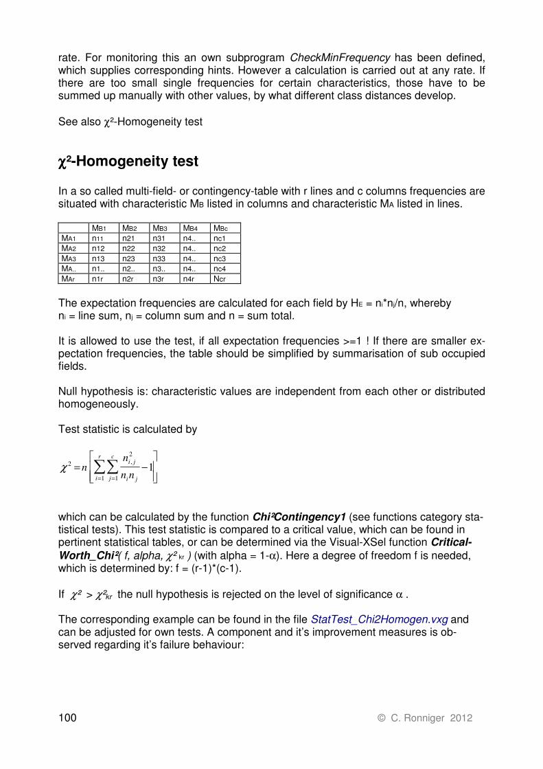
100 © C. Ronniger 2012
rate. For monitoring this an own subprogram CheckMinFrequency has been defined, which supplies corresponding hints. However a calculation is carried out at any rate. If there are too small single frequencies for certain characteristics, those have to be summed up manually with other values, by what different class distances develop.
See also χ²-Homogeneity test
χχχχ²-Homogeneity test In a so called multi-field- or contingency-table with r lines and c columns frequencies are situated with characteristic MB listed in columns and characteristic MA listed in lines. MB1 MB2 MB3 MB4 MBc
MA1 n11 n21 n31 n4.. nc1
MA2 n12 n22 n32 n4.. nc2
MA3 n13 n23 n33 n4.. nc3
MA.. n1.. n2.. n3.. n4.. nc4
MAr n1r n2r n3r n4r Ncr
The expectation frequencies are calculated for each field by HE = ni*nj/n, whereby ni = line sum, nj = column sum and n = sum total. It is allowed to use the test, if all expectation frequencies >=1 ! If there are smaller ex-pectation frequencies, the table should be simplified by summarisation of sub occupied fields. Null hypothesis is: characteristic values are independent from each other or distributed homogeneously. Test statistic is calculated by
χ 2
2
11
1= −
==
∑∑nn
n n
i j
i jj
c
i
r,
which can be calculated by the function Chi²Contingency1 (see functions category sta-tistical tests). This test statistic is compared to a critical value, which can be found in pertinent statistical tables, or can be determined via the Visual-XSel function Critical-
Worth_Chi²( f, alpha, χ² kr ) (with alpha = 1-α). Here a degree of freedom f is needed, which is determined by: f = (r-1)*(c-1).
If χ² > χ²kr the null hypothesis is rejected on the level of significance α . The corresponding example can be found in the file StatTest_Chi2Homogen.vxg and can be adjusted for own tests. A component and it’s improvement measures is ob-served regarding it’s failure behaviour:

© C. Ronniger 2012 101
Starting
constr.
Measure 1 Measure 2
Failure after 1 week
14 22 32
Failure after 2 weeks
18 16 8
Failure after 3 weeks
8 2 2
Question is, if the measures have a temporal influence on the failure behaviour. χ² re-
sults 17,04, the critical value χkr is for the level of significance 0,05 and the degree of
freedom 4 χ4,0,95 = 9,46 and therefore smaller than χ², that means there is no independ-ence of characteristics, a temporal influence on the failure behaviour does exist (there is no influence on the null hypothesis).
See also χ²-Test of goodness of fit und χ²- Multi field test
χχχχ²- Multi field test Several samples of a population are compared. The null hypothesis is: the mean num-ber of errors per unit is equal to the complete population. The so called contingency table looks like following: Population i 1 2 ... k Sampling volume n1 n2 ... nk
Number of errors in a sample
x1 x2 ... xk
The test statistic is determined by:
χ 2
2
1
=
−
=∑
x nx
n
nx
n
i i
ges
ges
i
ges
ges
i
k
with x xges ii
k
==∑
1
and n nges ii
k
==∑
1
which also can be calculated by the visual-XSel function Chi²Contingency3 (see func-
tions category statistical tests). χ² is compared to a critical value, which can be found in pertinent statistical tables, or can be determined via the Visual-XSel function Critical-

102 © C. Ronniger 2012
Worht_Chi²( f, alpha, χ² kr ) (with alpha = 1-α). Here a degree of freedom f is needed, which is determined by: f = k-1. The example file is StatTest_Chi2Multifield.vxg and can easily be adjusted for own evaluations. The same method is used for the template StatTest_Defects_2Samples_Contingency.vxg
If χ² > χ² kr , the null hypothesis is rejected on the level of significance.
See also χ²-Homogeneity test
Binomial-test The binomial distribution describes the number of faulty unities in random checks. The number of faulty unities in the random check can be used for a monitoring of the portion of faulty unities in the total population The likelyhood density is:
xnxpp
x
nh
−−
= )1(
x : variable n : number of samples p : relative ratio of faulty parts
The two-sided confidence level for checked
faults
on
np = is:
)(2
)1(42
)1(
)1(
2/1
2
2/12/1
2
2/1
2/1,2,1
2/1,2,1
α
ααα
α
α
−
−−−
−
−
+
−+−+=
++−
+=
un
pnpuuunp
Fxxn
Fxp
ooo
ff
ff
low
with f1= 2(x+1) and f2 = 2(n-x)
)(2
)1(42
)1( 2/1
2
2/12/1
2
2/1
2/1,2,1 α
ααα
α −
−−−
− +
−+++=
+−+=
un
pnpuuunp
Fxnx
xp
ooo
ff
up
with f1= 2(n-x+1) and f2 = 2x
The one-sided confidence level is:
α
α
−
−
++−
+=
1,2,1
1,2,1
)1(
)1(
ff
ff
obFxxn
Fxp
with f1= 2(x+1) and f2 = 2(n-x)
The hypothesis m events are equal po will be rejected if Z > u1-α/2
)1( oo
o
ppn
pnmZ
−
−=

© C. Ronniger 2012 103
As a test for a hypothesis whether a given faulty portion is within the confidence area lies is the template StatTest_Defects_1Sample_to_Specification.vxg.
Kolmogorov-Smirnov-Assimilation test The Kolmogorov-Smirnov-Assimilation Test (short KS-Test) check the assimilation of an observed distribution to any expected distribution. Especially at existence of small sam-pling volumes the KS-Test detects rather variances from the normal distribution. In gen-
eral distribution irregularities better can be proved via χ²-Test. The KS-Test also can be used for continuous and for discrete distributions. The null hypothesis is tested: The sample is descended from a known distribution. For each value the relative cumulative frequencies are compared and the maximum differ-ence value is used as test statistic Tprüf .
prüf
B E
TH H
n=
−max
This test statistic is compared to a critical value, which can be found in pertinent statisti-cal tables, or can be determined via the Visual-XSel function CriticalWorth_KS( n, al-
pha, Tkr ) (with alpha = α ).
If Tprüf > Tkr the null hypothesis is rejected on the level of significance α . The example file is called StatTest_KolmogSmirnov_Assim.vxg, which can easily be used for own data. In this file the number of points of a cube is checked. Of course the same number is expected for all six sides, but there are coincidental variances. So the maximum variance of cumulative frequencies is compared to an equal distribution. This does not exist in Visual-XSel and therefore has to be defined as an own subprogram (DistribEqual). If e.g. there is a test for another evaluation versus a normal distribution, the DistribEqual has to be exchanged to DistribNormal (see functions category statisti-cal distributions).
Shapiro-Wilk test The Shapiro-Wilk test, proposed in 1965, calculates a W statistic that tests whether a random sample, x1, x2, ..., xn comes from (specifically) a normal distribution (null hy-pothesis). The w statistic is calculated as follows:
2
2
)1( sn
bw
−=
∑=
=n
i
ii xab1
The null hypothesis is rejected on a significance level α if w < wkrit . The a weights and the critical wkrit can be found in the literature. The alternative to this is to use a following test value T:

104 © C. Ronniger 2012
−−
++=w
wTtest
1ln
εδγ
The coefficients γ, δ and ε can be found also in the literature. The advantage of Ttest is, that the result can be compared directly with the u-value of the normal distribution (quantile of the standardized normal distribution). If Ttest<-1,645 the null hypothesis is
rejected (significance level α=0,05).
To use this test there is available the template:
StatTest_ShapiroWilk_normal_distribution.vxg
Anderson-Darling test of normal-distribution The Anderson Darling test checks the null hypothesis that the sample data comes from a normal-distributed population. This test is suitable for small and big samples size and considers in particular the edge areas of the data.
∑=
+Φ+Φ−−=n
i
uun
nA1
i-1ni )))(-ln(1))((ln(1)-(2i1
²
with
s
xxu i
i
−=
and )( iuΦ for the probability of the u-values of the normal-distribution.
With the help of A² there is defined the z-value:
++=2
25,275,01²
nnAz
The following table shows the p-value for the adequate z-value:
The p-value is the confidence level for the alternative hypothesis that the data are not normal-distributed. Thererfore the data is normal-distributed if the p-value > 0.05. The adequate template for this method is StatTest_Normal_Distribution_Anderson_Darling.vxg. Literature /23/ .. /24/
z ≤ 0, 2 p-value = 1 − exp(−13,436 + 101,14z − 223,73 z2)
0, 2 < z ≤ 0,34 p-value = 1 − exp(−8,318 + 42,796z − 59,938 z2)
0, 34 < z ≤ 0, 6 p-value = exp (0,9177 − 4, 279z − 1,38 z2)
0, 6 < z p-value = exp(1,2937 − 5, 709z + 0,0186 z2)

© C. Ronniger 2012 105
t-test for two samples This test checks the null hypothesis: The mean values of both samples are equal. From s and x of both samples the test statistic tpr is calculated in subprogram t_Test of the file StatTest_t.vxg . (The subprogram is also directly available as tTest in the selection functions category Statistical Tests).
tx x
spr
d
=−1 2
with
ss
n
s
nd = +1
2
1
2
2
2
Degree of freedom f is determined by:
fc
n
c
n
=
−+
−−
1
1
1
1
2
1
2
2
( )
with cs
n sd
= 1
2
1
2
This test statistic is compared to a critical value tkr, which can be found in pertinent sta-tistical tables, or can be determined via the function CriticalWorth_t( f, alpha, tkr ) (with
alpha = 1 - α/2 ).
If tpr > tkr the null hypothesis is rejected on the level of significance α . Strictly speaking a F-Test should be executed before each t-test, to confirm the precon-ditioned equality of variances. If the null hypothesis of the variances is rejected, the t-test delivers wrong values. The double sided confidence range is determined by: x x t s x x t sf d f d1 2 1 2 1 2 1 2 1 2− − ≤ − ≤ − +− −, / , /( )α αµ µ
See also t-Test for Comparison of a Sample with a Default U-Test for two Samples (distribution indepentend)

106 © C. Ronniger 2012
Test for comparison of one sample with a default value This test check the null hypothesis: the mean value of the sample corresponds to an default mean value µo. The test statistic is determined by
ux
npr
o=− µ
σ
This test statistic is compared to the u-value at an alleged level of significance α. The u-
value can be determined in the category statistical distributions (with alpha = 1 - α/2 ) by the function InvNormal(alpha, uα ). The null hypothesis is rejected if for the double sided test-case µ = µo is:
u upr kr>
Often there is the one-sided test questioned, for example if the mean is greate than an upper or an lower limit. The tabel shows the possible problems:
Ho H1 Ho is rejected if
ox µ= ox µ<> 2/1 α−> uu pr
ox µ≥ ox µ< α−−< 1uu pr
ox µ≤ ox µ> α−> 1uu pr
If σ is not known and has to be estimated from s, the test statistic results with
tx
snpr
o=− µ
The null hypothesis is rejected, if for the double sided test-case µ = µo is:
t tpr kr>
The critical t-value can be found in pertinent statistical tables, or can be determined via
the Visual-XSel function CriticalWorth_t( f; alpha; tkr ) (with f = n-1; alpha = 1 - α/2 ). See also t-Test for two samples The adequate template for this method is StatTest_t_1Sample.vxg

© C. Ronniger 2012 107
U-test for two samples This test after Wilcoxon, Mann and Whitney tests over the order whether the median values of two spot checks are equal. It is the distribution-independent counterpart to the t-Test and insensitively against different variances. The U-Test is therefore put in if no normal-distribution can be presupposed. To the calculation of the test value U, one brings the n1 and n2 to big spot checks in a common ascending order, with which is noted to each position-number, from which comes the two spot checks it. Example: Following spot checks are available:
Spot 1
7 1 4 2 2 3 6 4 0 4 8 4 9 5 2
Spot 2 3 5 6
1 0 1 7 1 8 2 0 3 9
In the common order emerges with the ranked numbers for the spot check 1 and 2 the values represented right with the position-sums R1 and R2. A test value can be deter-mined for each spot check:
111
2112
)1(R
nnnnU
+=
2
22
2122
)1(R
nnnnU
+=
The in the end required test value U the smaller of the two, in this case U=U1=11, that is compared against a critical value of Ucrit, is is in the presentation-file StatTest_U_Wilcoxon.vxg In case of the fact that there are the same values one speaks of binding. In this case a middle rank is formed in each case and the rank sums are provided with a correction factor. More information will be found in the literature. If U < Ucrit, the hypothesis that the median values of the spot check are equal is re-jected. See also t-Test for Two Samples
3 5 6 7
1 0 1 4 1 7 1 8 2 0 2 2 3 6 3 9 4 0 4 8 4 9 5 2
Spot 1
4
6
1 0 1 1
1 3 1 4 1 5 1 6
Σ = 8 9
Spot 2 1 2 3
5
7 8 9
1 2
Σ = 5 3

108 © C. Ronniger 2012
F-test The variances of two samples are tested. The null hypothesis is: the samples are descended from the same population. The test statistic is formed by:
Fs
spr = 1
2
2
2
whereby the larger variance is always in the counter, so that Fpr >= 1 . This value is compared to the critical F-value, which can be found in pertinent statistical tables, or can be determined via the Visual-XSel function CriticalWorth_F( f1, f2, alpha, Fkr ) ( with
alpha = 1-α/2 ). The degree of freedom f1 and f2 results from f1 = n1 - 1 and f2 = n2 - 1, whereby the index 1 always refers to the sample value with the larger variance.
If Fpr > Fkr the null hypothesis is rejected on the level of significance α . The example file is called StatTest_F.vxg, which can be used for own evaluations. See also Rank Dispersion Test
Outlier test With this test a series can be checked on one or several outliers. Precondition is that data are normal distributed. Sequentially this test can be repeated as long as no outlier can be determined any more. After ascertainment of an outlier this has to be removed from the series, before the next test is called. The test measurement is:
Tn
n
x x
spr
i
i
n
=−
−
=∑
( )1 21
4
which will be compared to a critical value Tkr . The test is carried out within the available function OutlierTest in the category statistical tests. What will be supplied back is the index of the line in the matrix (resp. table), in which an outlier has been ascertained. In the example file StatTest_Outlier.vxg there is a program, which eliminates correspond-ing values from a series, before the next test is carried out.

© C. Ronniger 2012 109
After run of this program all outliers will be written on the right side besides the series.
Count( T1; 0; 1; 0; 1000 ;n)
OutlierTest( T1; 0; 1; n;WIdx)
WIdx 1 -<>True
False
T1 1,WIdx T1 0,WIdx=
T1 0,WIdx EMPTY=
Stop
Start

110 © C. Ronniger 2012
Balanced simple Analysis of Variance Expectation values of several samples (number k) with same volume n are compared. The null hypothesis is: all expectations values are equal. Precondition for the test is that
σi = σ . The test statistic is formed by:
Fn s
spr
x=2
2
with
sk
x xx ii
k
2
1
21
1=
−−
=∑ ( )
xk
xii
k
==∑
1
1
sk
si
i
k
2 2
1
1=
=∑
whereby xi and si of the respective samples are assumed. This value is compared with the critical F-value, which can be found in pertinent statistical tables, or can be deter-
mined via Visual-XSel function CriticalWorth_F( f1, f2, alpha, Fkr ) ( with alpha = 1-α ). The degree of freedom f1 and f2 results from f1 = k-1 and f2 = k(n-1).
If Fpr > Fkr the null hypothesis is rejected on the level of significance α . The double sided confidence belt is determined by the critical t-values (CriticalWorht_t(
f2; alpha; t) with alpha = 1-α/2 to
x ts
nx t
s
ni f i f− ≤ ≤ +− −2 1 2 2 1 2, / , /α αµ
The corresponding example file is StatTest_BalVariance_Analysis.vxg, which easily can be adjusted for own evaluations. See also Bartlett Test

© C. Ronniger 2012 111
Bartlett-test More than two populations are compared. The null hypothesis is: all variances are equal. Precondition for test application is that ni>=5 . The test statistic results to:
χ pr i
ii
k
cf
s
s
2
2
21
1=
=∑ ln( )
with f ni i= −1, f fges i
i
k
==∑
1
sf
f sges
i ii
k
2 2
1
1=
=∑
ck f fii
k
ges
= +−
−
=
∑11
3 1
1 1
1( )
with k = number of populations = number of samples. xi and s²i of the respective sam-ples are taken for granted, resp. have to be calculated before.
χ²pr is compared to a critical value, which can be found in pertinent statistical tables, or
can be determined via Visual-XSel function CriticalWorth_Chi²( f, alpha, χ² kr ) (with
alpha = 1-α). Here a so called degree of freedom f is needed, which is determined by: f = k-1.
If χ²pr > χ² kr , the null hypothesis has to be rejected on the level of significance α. The example file is StatTest_Bartlett.vxg and can easily be adjusted for own evalua-tions. See also : Balanced Analysis of Variance

112 © C. Ronniger 2012
Rank dispersion test according to Siegel and Tukey At this test two samples are compared to each other, where you cannot assume that they are normal distributed. The test is free of distribution. The null hypothesis Ho is: both samples belong to a common population. While executing the tests both samples are gathered up in a series and sorted. The smallest value gets ranking 1, the both largest values get descending rankings 2 and 3, the next smallest values 4 and 5 ascending and so on. If there is an odd number of ob-servations, the middle observation gets no ranking so that the highest ranking always is an even number. For distinguishing which value belongs to which sample, those are indicated before (value 1 for sample 1 and value 2 for sample 2). Afterwards the total of ranking numbers for each sample is formed and issued. The more the ranking number totals distinguish, the less it is probable that they belong to the same population. In the following table the lower and upper limits of ranking numbers are shown
Ho is rejected (α=0,05 double sided resp. α=0,025 one sided) if R1 or R2 exceeds or falls below or reaches the lower respectively upper barrier. The file StatTest_Rank_Dispersion.vxg is used as submission, which can be adjusted for own evaluations. For following both samples R1=134 and R2=76 have been deter-mined. As it can be seen in the above table that R1<78 and R2>132 . So the null hy-pothesis has to be rejected, there is no dispersion difference.
Spot 1 Spot 2 10,1 15,3
7,3 3,6 12,6 16,5
2,4 2,9 6,1 3,3 8,5 4,2 8,8 4,9 9,4 7,3
10,1 11,7 9,8 13,1
n1->
n2=n1
n2=n1+1
n2=n1+2
n2=n1+3
n2=n1+4
n2=n1+5
4
10
11
12
13
14
14
26
29
32
35
38
42
5
17
18
20
21
22
23
38
42
45
49
53
57
6
26
27
29
31
32
34
52
57
61
65
70
74
7
36
38
40
42
44
46
69
74
79
84
89
94
8
49
51
53
55
58
60
87
93
99
105
110
116
9
62
65
68
71
73
76
109
115
121
127
134
140
10
78
81
84
88
91
84
132
139
146
152
159
166

© C. Ronniger 2012 113
Test of an best fit straight line Any best fit straight line is tested on linearity and gradient. This test is a summarisation of both single available submissions. The file StatTest_StraightLine.vxg is used as submission, which can be adjusted for own evaluations.
Test on equal regression coefficients Two series are tested on equal regression coefficients. There the following t-value is calculated,
( ) ( )
+
−+
−+−
−=
2121
22
212
1
21
11
4
22
xx
yxyx
QQnn
nsns
bbt
which is compared to a critical tkrit on the level of significance α=5% . Both regression coefficients are equal, if t < |tkrit| . The file StatTest_2_RegrCoeff.vxg is used as submission, which can be adjusted for own evaluations.
Linearity test Tests a series on linearity. See also Test of an Equation Straight line The data entered in the table page T1 are categorised via the function Classify and writ-ten in the table page T2. All occurring values within one class are entered here horizon-tally. Out of this matrix a F-value is calculated:
( )
( )∑∑
∑
= =
=
−−
−−
=k
i
n
j
iji
k
i
iii
i
YYkn
YYnk
F
1 1
2,
1
2
ˆ1
ˆ2
1
which will be compared on the level of significance α=5%. If F < Fkrit (k-2,n-k), there is a significant linearity. The file StatTest_Linearity.vxg is used as submission, which can be adjusted for own evaluations.

114 © C. Ronniger 2012
Gradient test of a regression
It is tested, if the gradient of a equation straight line significantly differs from 0. A t-value
is formed as quotient of a regression coefficient b to it’s variation. From this the value α is determined from the student’s t-distribution and compares this to the level of signifi-
cance α=5%. If α < 5%, significantly a gradient > 0 does exist. See also Test of an Equation Straight Line, where also this test is included. The file StatTest_Gradient_Regression.vxg is used as submission, which can be ad-justed for own evaluations.
Independence test of p series of measurements Test the correlation-coefficients on mutual independence. For example this test is used to check at a multiple regression, if all variables are necessary. Data are entered in the table page T1. First the so called correlation matrix is formed (stands after start of program in table page T2). There the correlation coefficients r are listed in pairs in every possible combination of series of measurements. A limit R‘ is de-
termined on the level of significance α via student’s t- distribution:
2
lim
lim1
2'
it
itr
nrR
−
−=
and iterativly rlimit is calculated, which is compared to the maximum founded correlation
coefficient. If rmax < rlimit, then on the level α=5% no pair of series of measurements sig-nificantly depends on each other. The file StatTest_Independence_p_Series.vxg is used as submission, which can be adjusted for own evaluations.

© C. Ronniger 2012 115
9. Normal-distribution The normal distribution is the most frequently and most common form of the probability distribution dar. The normal-distribution is relevant when random events affect a proc-ess. Many natural, economic and engineering processes can be achieved by the normal distribution, either exactly or at least at a very good approximation (especially processes that act independently to factors in different directions).
In the top histogram the data is grouped in suitable classes. The Gaussian-curve
represents the ideal probability-density of this histogram, if one have endless data and a
absolute small class-width. In the cummulative probability chart below one can read the
sum of values, which are less or equal to x. That is the area under the Gaussian curve.
The mean is the probability at 50% (here at x = 0). The confidence interval of the mean
value is
EF − ���/ "√� ≤ EF ≤ EF + ���/ "
√�
Merkmal
-1.0 -0.8 -0.6 -0.4 -0.2 0.0 0.2 0.4 0.6 0.8 1.0
%
Su
mm
en
wa
hrs
ch
ein
lic
hk
eit
0.1
0.3
1
3
10
20
40
60
80
90
96
99.9
Merkmal
-1.0 -0.8 -0.6 -0.4 -0.2 0.0 0.2 0.4 0.6 0.8 1.0
Hä
ufi
gk
eit
0
50
100
150
200
%
Re
lati
ve
Hä
ufi
gk
eit
0
5
10
15
20
2
2
1
2
1
−−
= s
xx
ehσπ
x : Variable µ : meand
σ : Standard-deviation
dx
x
s
xx
eH ∫∞−
−
−
=
2
2
1
2
1
σπ
Integral not solvable
x
Fre
uque
ncy
Cum
mula
tive p
rob
abili
ty
Rela
tive
pro
babili
ty
Attribute x
Attribute x
t1-α/2 : Quantile of the Student-distribution with the significance
α, it the real standard-deviation in not known.

116 © C. Ronniger 2012
The slope of the straight line represents the scatter (standard-deviation) of the data. At
sx ± there is 16%, respectively 84% of the data. Both charts have their own advantag-
es. In the histogram a mixed distribution can be detected easily if there are more than
one caps. In the cummulative probability chart one can see each data-point and the
deviation from the straight-line is a non-regularity to the normal-distribution.
± 1σ
± 2σ
± 3σ
± 4σ
± 5σ
± 6σ
68,27%
95,45%
99,73%
99,9937%
99,999943%
99,9999998%
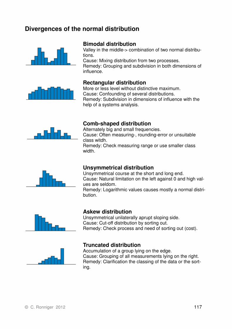
© C. Ronniger 2012 117
Divergences of the normal distribution
Bimodal distribution Valley in the middle-> combination of two normal distribu-tions. Cause: Mixing distribution from two processes. Remedy: Grouping and subdivision in both dimensions of influence.
Rectangular distribution More or less level without distinctive maximum. Cause: Confounding of several distributions. Remedy: Subdivision in dimensions of influence with the help of a systems analysis.
Comb-shaped distribution Alternately big and small frequencies. Cause: Often measuring-, rounding-error or unsuitable class witdh. Remedy: Check measuring range or use smaller class width.
Unsymmetrical distribution Unsymmetrical course at the short and long end. Cause: Natural limitation on the left against 0 and high val-ues are seldom. Remedy: Logarithmic values causes mostly a normal distri-bution.
Askew distribution Unsymmetrical unilaterally aprupt sloping side. Cause: Cut-off distribution by sorting out. Remedy: Check process and need of sorting out (cost).
Truncated distribution Accumulation of a group lying on the edge. Cause: Grouping of all measurements lying on the right. Remedy: Clarification the classing of the data or the sort-ing.

118 © C. Ronniger 2012
10. Statistical factors
Factor Definition Description
DF Degrees of Freedom For statistical tests
N Number of populations e.g. production quantity
n Sampling volume of degree of freedom or number of independent trials
In general : number of parts
f Degree of freedom for statistical tests
k Number of categories
i Ordinal number In general :running index
H Frequency Mostly in %
xo Reference value of population Mostly approximated mean value
x Mean value of a sample ∑
=
=n
i
ixn
x1
1
∆x Class size In general : increment
µ Mean value of population
R Range R = xmax - xmin
s Standard deviation of sample ( )s
x x
n=
−
−∑
2
1
s² Variance of sample
σ Standard deviation of population
p Probability of success
b Form parameter at Weibull Gradient of equation straight line in Weibull-Net
t Life cycle of variable at Weibull route, length of use, load changes and so on
T Characteristical service life at Weibull
For 63.2% failure frequency
w Weighting Number of alleged value
α Level of significance for statistical check
The transfer parameter alpha often is
alpha = 1- α resp. 1 - α/2 for double sided tests
z Number of variables or factors

© C. Ronniger 2012 119
11. Literature
/1/ Keki Bhote World Class Quality American Management Association, New York 1991 ISBN 0-8144-5053-9
/2/ Georg E.P. Box, Norman R. Draper Empirical Model Building and Response Surfaces Wiley, New York 1987 ISBN 0-471-81033-9
/3/ Wilhelm Kleppmann Taschenbuch Versuchsplanung Hanser Verlag München 1998 ISBN 3-446-19271-9
/4/ H. Ulrich, G.J.B Probst Anleitung zum ganzeitlichen Denken und Handeln Haupt 1991
/5/ Lothar Sachs Angewandte Statistik Springer-Verlag Berlin 1983 ISBN 3-540-12800-X
/6/ Peterson Grundlagen der Statistik und der statistischen Versuchsplanung Ecomed Landsberg /Lech 1991 ISBN 3-609-75520-2
/7/ Statistik Lehr- und Handbuch der angewandten Statistik Hartung, Elpelt, Klösner Oldenburg Verlag München Wien ISBN 3-486-24984-3
/8/ Multivariate Statistik Lehr- und Handbuch der angewandten Statistik Hartung, Elpelt, Klösner
Oldenburg Verlag München ISBN 3-486-21430-6
/9/ Neuro- Fuzzy-Systeme Borgelt, Klawonn, Kruse, Nauck Vieweg 2003, ISBN 3-528-25265-0 /10/ Optimierung vielparametriger Systeme in der Kfz-Antriebsentwicklung Alexander Mitterer Fortschritt-Bereicht VDI Reihe 12 Nr. 434, ISBN 3-18-343412-1

120 © C. Ronniger 2012
/11/ Praktische Einführung in Neuronale Netze. Allesandro Mazzetti Hannover: Heise, 1992
/12/ Körpereigene Drogen Josef Zehentbauer Artemis & Winkler Verlag, 1993, ISBN 3-7608-1935-4
/13/ Wold, H. (1966)
Nonlinear Estimation by Iterative Least Squares Procedures, in: David, F. N. (Hrsg.), Festschrift for J. Neyman: Research Papers in Statistics, London 1966, 411-444.
/14/ S. World, E. Johannson, M. Cocchi, 3D QSAR in Drug Desing;
Theory, Methods, and Applications, ESCOM, Leiden, Holland, 1993, pp. 523-550.
/15/ Praxisleitfaden Qualität Walter Jahn, Lorenz Braun Hanser Verlag 2006, ISBN-10: 3-446-40616-6 /16/ Taschenbuch der Statistik Rinne Verlag Harri Deutsch 2003, ISBN 3-8171-1695-0 /17/ Formelsammlung zu den statistischen Methoden des Q-Managements DGQ-Band 11-05, Graeb ISBN 3-410-32877-7 /18/ Multivariate Datenanalyse Waltraud Kessler WILEY-VCH Verlag GmbH & Co KGaA ISBN 978-3-527-31262-7 /19/ Statistics for Experiments Box & Hunter Wiley Series ISBN 0-471-09315-7 /20/ Six Sigma +Lean Toolset Lunau, Roenpage, Staudter, Meran, John, Beernaert Springer ISBN 10-3-540-46054-3 /21/ Design for Six Sigma+Lean Toolset Lunau, Mollenhauer, Staudter, Meran, Hamalides, Roenpage, von Hugo
Springer ISBN 978-3-540-69714-5

© C. Ronniger 2012 121
/22/ Design for Six Sigma Gamweger, Jöbstl, Strohmann, Suchowerskyj Hanser Verlag 2009 ISBN 978-3-446-41454-9 /23/ Groß, J.
A Normal Distribution Course. Peter Lang Verlag 2004 ISBN 978-3631529348
/24/ Stephens, M.A.
Tests based on EDF statistics. D'Agostino, R.B. and Stephens, M.A., eds.: Goodness-of-Fit Techniques. Marcel Dekker, New York 1986
/25/ Thode Jr., H.C. Testing for Normality. Marcel Dekker, New York 2002
/25/ Thode Jr., H.C.
Testing for Normality. Marcel Dekker, New York 2002
/26/ Graf, Henning, Stange, Wilrich
Formeln und Tabellen der angewandten math. Statistik Springer Verlag 1987 ISBN: 978-3-540-16901-7
/27/ Measurement System Analysis MSA Fourth Edition 7/2010
ISBN# 978-1-60-534211-5
/28/ Measurement System Capability – Reference Manual September 2002, Version 2.1 D/E

122 © C. Ronniger 2012
12. Index 3 levels 32 3D-chart .............................................. 61 agglomerative ..................................... 71 Analyis of Means ................................ 24 Analysis of Variance ........................... 19 Anderson DarlingTes ........................ 104 ANOM 22 ANOVA 19, 22 ANOVA multifactors ............................ 22 ANOVA regression model ................... 49 ANOVA two samples .......................... 20 appraiser ............................................. 95 appraiser variation .............................. 96 ARM 96 Average-Range-Method ..................... 96 balanced simple ANOVA .................. 110 Bartlett-Test ...................................... 111 Bhote 119 bimodal distribution ........................... 117 binomial distribution .......................... 102 binomial-test ..................................... 102 Box 119 Box & Hunter .................................... 120 Box-Behnken ...................................... 32 Box-Cox .............................................. 56 boxplot 87 Bravais - Pearson ............................... 38 capability ............................................. 10 capability indices................................. 91 capability studies ................................ 94 categorial characteristic ...................... 73 categorical factors............................... 47 CCC 32 CCD 33 CCF 32 Central Composite Circumscribed ...... 32 Central composite Design ................... 26 Central Composite Design .................. 31 Central Composite Face ..................... 32 central point ........................................ 32 central points ...................................... 33 chemical liquids .................................. 34 Chi² Homogeneity Test ..................... 100 Chi² Multi Field Test .......................... 101 Chi² test of goodness of Fit ................. 99 city-block distance .............................. 70 cluster analysis ................................... 70 coefficient of determination ................. 49
test of .............................................. 52 coefficients .......................................... 76 comb-shaped distribution .................. 117 comparison B versus. C ...................... 13 component .......................................... 76 components .................................. 74, 79 Components Search ............................. 8 condition number ................................ 54 confidence interval
linear regression .............................. 40 response ......................................... 54
Confidence interval regression coefficient ...................... 54
confidence intervals ............................ 33 confidence level ................................ 102 confounding ........................................ 28 constant .............................................. 45 contingency table ................ 99, 100, 101 correlating data ................................... 76 correlation ........................................... 38 correlation coefficient .......................... 40 correlation coeffizicient ....................... 38 correlation loading plot ........................ 79 correlation matrix .................... 39, 55, 70 Cpk 91 CRGRAPH ............................................ 6 cubic 26 cubic model......................................... 85 curve-diagram ..................................... 58 data reduction ..................................... 71 defects 103 Defects two samples ......................... 102 degree of performance ....................... 63 degrees of freedom ....................... 48, 49 dendrogram ........................................ 72 design characteristics ......................... 94 Design of Experiment ......................... 26 determinant ......................................... 33 deviation ............................................. 64 discrete regression ............................. 64 distance matrix .................................... 71 D-Optimal...................................... 27, 48 download .............................................. 6 Draper 119 effect chart .......................................... 59 eigenvalue .................................... 54, 74 eigenvectors ....................................... 74 ellipse 74, 79
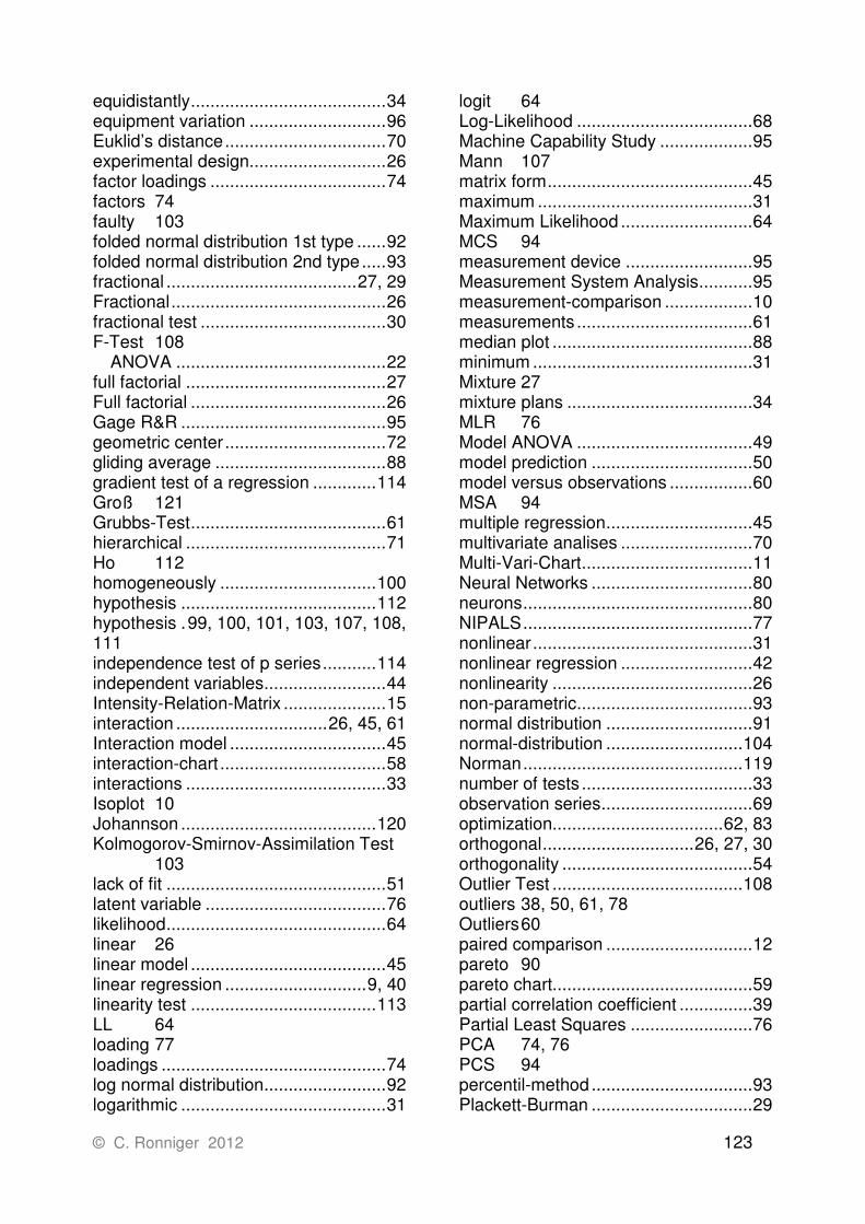
© C. Ronniger 2012 123
equidistantly ........................................ 34 equipment variation ............................ 96 Euklid’s distance ................................. 70 experimental design ............................ 26 factor loadings .................................... 74 factors 74 faulty 103 folded normal distribution 1st type ...... 92 folded normal distribution 2nd type ..... 93 fractional ....................................... 27, 29 Fractional ............................................ 26 fractional test ...................................... 30 F-Test 108
ANOVA ........................................... 22 full factorial ......................................... 27 Full factorial ........................................ 26 Gage R&R .......................................... 95 geometric center ................................. 72 gliding average ................................... 88 gradient test of a regression ............. 114 Groß 121 Grubbs-Test ........................................ 61 hierarchical ......................................... 71 Ho 112 homogeneously ................................ 100 hypothesis ........................................ 112 hypothesis . 99, 100, 101, 103, 107, 108, 111 independence test of p series ........... 114 independent variables ......................... 44 Intensity-Relation-Matrix ..................... 15 interaction ............................... 26, 45, 61 Interaction model ................................ 45 interaction-chart .................................. 58 interactions ......................................... 33 Isoplot 10 Johannson ........................................ 120 Kolmogorov-Smirnov-Assimilation Test 103 lack of fit ............................................. 51 latent variable ..................................... 76 likelihood ............................................. 64 linear 26 linear model ........................................ 45 linear regression ............................. 9, 40 linearity test ...................................... 113 LL 64 loading 77 loadings .............................................. 74 log normal distribution ......................... 92 logarithmic .......................................... 31
logit 64 Log-Likelihood .................................... 68 Machine Capability Study ................... 95 Mann 107 matrix form .......................................... 45 maximum ............................................ 31 Maximum Likelihood ........................... 64 MCS 94 measurement device .......................... 95 Measurement System Analysis ........... 95 measurement-comparison .................. 10 measurements .................................... 61 median plot ......................................... 88 minimum ............................................. 31 Mixture 27 mixture plans ...................................... 34 MLR 76 Model ANOVA .................................... 49 model prediction ................................. 50 model versus observations ................. 60 MSA 94 multiple regression .............................. 45 multivariate analises ........................... 70 Multi-Vari-Chart ................................... 11 Neural Networks ................................. 80 neurons ............................................... 80 NIPALS ............................................... 77 nonlinear ............................................. 31 nonlinear regression ........................... 42 nonlinearity ......................................... 26 non-parametric .................................... 93 normal distribution .............................. 91 normal-distribution ............................ 104 Norman ............................................. 119 number of tests ................................... 33 observation series ............................... 69 optimization................................... 62, 83 orthogonal ............................... 26, 27, 30 orthogonality ....................................... 54 Outlier Test ....................................... 108 outliers 38, 50, 61, 78 Outliers 60 paired comparison .............................. 12 pareto 90 pareto chart......................................... 59 partial correlation coefficient ............... 39 Partial Least Squares ......................... 76 PCA 74, 76 PCS 94 percentil-method ................................. 93 Plackett-Burman ................................. 29

124 © C. Ronniger 2012
PLS 76 polynom .............................................. 42 prediction measure ............................. 50 Principle Component Analysis ............ 74 priority matrix ...................................... 16 Process Capability Study .................... 94 pseudo-R² ........................................... 64 pure Error ........................................... 51 p-value 104 Q² 50 quadratic ....................................... 26, 31 qualitative factors ................................ 47 R&R 95 R² 49 Rank Dispersion Test ....................... 112 ranking 112 Rayleigh-distribution ........................... 93 rectangular distribution ..................... 117 reduction ............................................. 74 Red-X 7 regression ........................................... 40 regression coefficients ...................... 113
test of .............................................. 52 regression model ................................ 76 regression types ................................. 42 repeatability .................................. 95, 96 Repetitions .......................................... 47 reproducibility ............................... 52, 95 residual-matrix .................................... 77 residues .......................................... 9, 60 Resolution ........................................... 28 RMS 54 root mean squared .............................. 54 Sample size ........................................ 47 scatter bars ......................................... 86 scatter plot ............................................ 9 score 74, 76 score plot ............................................ 78 Screening ........................................... 28 screening plans................................... 50 screening-plans .................................. 29 Shainin 7 Shapiro-Wilk test............................... 103 significant ............................................ 47 Spearman ........................................... 38
specification limit ................................. 93 spread 77 square 31 squared terms ..................................... 45 standard deviation .............................. 54 standard plans .................................... 26 standardize ......................................... 55 star 32 statistical charts .................................. 58 statistical factors ............................... 118 Statistical Tests ................................... 99 Stephens .......................................... 121 straight line ........................................... 9 Sum of Squares .................................. 64 Taguchi ........................................... 7, 26 Taguchi plans ..................................... 30 temporal influence .............................. 11 test regression coefficients ............... 113 theoretical distribution ......................... 99 Thode 121 tolerance ............................................. 95 tolerance parallelogram ........................ 9 topology .............................................. 80 training-algorithm ................................ 82 transformation ..................................... 31 transformed......................................... 50 triangle 34 Truncated distribution ....................... 117 Tschebyscheff distance ...................... 70 t-Test for two Samples ...................... 105 t-test one sample with default value .. 106 Type-1 Study ...................................... 95 Type-2 Study ...................................... 95 Type-3 Study ...................................... 96 U-Test 107 variance ...................................... 79, 111 vector 45 VIP 78 Visual-XSel ........................................... 6 weight matrix ....................................... 76 Whitney ............................................. 107 Wilcoxon ........................................... 107 Wold 76, 78, 120 World 120

© C. Ronniger 2012 125

126 © C. Ronniger 2012
Edition 12 Curt Ronniger
© 2012


