C 1 Quadratic Interpolation of Meshes David Eberly, Geometric Tools, Redmond WA 98052 https://www.geometrictools.com/ This work is licensed under the Creative Commons Attribution 4.0 International License. To view a copy of this license, visit http://creativecommons.org/licenses/by/4.0/ or send a letter to Creative Commons, PO Box 1866, Mountain View, CA 94042, USA. Created: March 2, 1999 Last Modified: April 7, 2018 Contents 1 Introduction 2 2 Mathematical Preliminaries 2 2.1 Barycentric Coordinates ....................................... 2 2.2 Inscribed Centers ........................................... 3 2.3 B´ ezier Triangles ............................................ 5 2.4 Derivatives .............................................. 6 2.5 Derivative Continuity ........................................ 7 3 Globally C 1 Quadratic Height Field of Form h = f (x 0 ,x 1 ) without Local Control 10 4 Globally C 1 Quadratic Height Field of Form h = f (x 0 ,x 1 ) with Local Control 15 5 The Algorithm for Graphs of f (x, y, z) 19 6 The Algorithm for Surfaces 22 1
Transcript
C1 Quadratic Interpolation of Meshes
David Eberly, Geometric Tools, Redmond WA 98052https://www.geometrictools.com/
This work is licensed under the Creative Commons Attribution 4.0 International License. To view a copyof this license, visit http://creativecommons.org/licenses/by/4.0/ or send a letter to Creative Commons,PO Box 1866, Mountain View, CA 94042, USA.
Created: March 2, 1999Last Modified: April 7, 2018
This document describes the Cendes-Wong algorithm [2] for interpolating arbitrary point sets with elements((xi, yi), f(xi, yi), fx(xi, yi), fy(xi, yi)) for 0 ≤ i < N . The interpolating function f(x, y) has continuousfirst-order derivatives. The points (xi, yi) are arbitrarily spaced. At each point (xi, yi) the user specifies thefunction value f(xi, yi) and its two first-order partial derivatives fx(xi, yi) and fy(xi, yi). The outline of thealgorithm is as follows.
1. Triangulation. The spatial points must be triangulated. Generally, one chooses a Delaunay triangula-tion; see [4].
2. Subdivison. Each triangle is subdivided into six triangles. The subdivision requires knowledge of theinscribed centers of the triangle and its three adjacent triangles.
3. Bezier net construction. Each subtriangle is further subdivided into four triangles. This subdivision isaffine and the partition is used to build a quadratic function via the Bezier triangle method describedin [3]. The quadratic function for a single triangle is, of course, a C1 function, but additionally theinterpolation is C1 at the vertices and edges shared with other triangles.
The interpolator accepts as input a spaital location (x, y) and returns as output the interpolated values forf(x, y), fx(x, y) and fy(x, y).
The reduced computation of this algorithm compared to that for cubic interpolators is attractive. Thesetup costs for the interpolation are assumed to be negligible compared to the cost of interpolation for alarge number of input points. Because the interpolation guarantees only C1 continuity, an application thatrequires C2 continuity must use a different interpolation algorithm. This is true, for example, when theapplication requires smoothly varying normal vectors or must compute surface curvatures.
The interpolation has local control. If the function or derivative values are modified at a single data point,then the affine subdivision of the triangles sharing the data point does not change, but the function values atthe control points generated by subdivision must be recomputed. If the spatial component of a single datapoint is modified, then the affine subdivisions of the triangles sharing the data point change. These changesare propagated to any immediately adjacent triangles of those which share the data point, but no farther.
I provide a generalization of the Cendes-Wong algorithm to graphs of functions f(x, y, z, w). The ideas workin general dimensions. I also mention how you can apply the ideas to a 2-dimensional manifold trianglemesh as long as you have a package to generate 2-dimensional surface parameters (automatically generatedtexture coordinates, so to speak).
2 Mathematical Preliminaries
2.1 Barycentric Coordinates
Let a triangle have vertices p0, p1 and p2. Any point p can be written as a linear combination of the trianglevertices,
p = u0p0 + u1p1 + u2p2, u0 + u1 + u2 = 1 (1)
2
The coefficients (u0, u1, u2) are the barycentric coordinates of the point p with respect to the triangle. If p isinside the triangle or on a triangle edge, we additionally know that ui ∈ [0, 1]. If p is outside the triangle,at least one of ui is negative. The definition is independent of dimension; the vectors can be in Rn for anyn ≥ 2.
Constructing u0, u1 and u2 is a matter of solving a system of linear equations. Subtracting p2 from theequation for p, using u2 = 1− u0 − u1 and grouping terms leads to
p− p2 = u0(p0 − p2) + u1(p1 − p2) (2)
The vectors p0 − p2 and p1 − p2 are linearly independent because they are two edges of the same triangle.The linear independence also guarantees the linear system has a unique solution for u0 and u1. Dot thesevectors with equation (2) to obtain the linear system of equations (p0 − p2) · (p0 − p2) (p0 − p2) · (p1 − p2)
(p0 − p2) · (p1 − p2) (p1 − p2) · (p1 − p2)
u0
u1
=
(p0 − p2) · (p− p2)
(p1 − p2) · (p− p2)
(3)
Although it is simple to solve the equation algrabraically, the solution can be written geometrically as
u0 =Area(p,p1,p2)
Area(p0,p1,p2), u1 =
Area(p0,p,p2)
Area(p0,p1,p2), u2 =
Area(p0,p1,p)
Area(p0,p1,p2)(4)
where Area(·, ·, ·) is the area of the triangle formed by the input points.
Given two points q0 and q1, the difference is a vector ∆ = q1 − q0. With respect to the aforementionedtriangle with vertices pi, let (u0, u1, u2) be the barycentric coordinates of q0 and let (v0, v1, v2) be thebarycentric coordinates of q1. Define di = ui − vi; then
∆ = q1 − q0
= (u0p0 + u1p1 + u2p2)− (v0p0 + v1p1 + v2p2)
= (u0 − v0)p0 + (u1 − v1)p1 + (u2 − v2)p2
= d0p0 + d1p1 + d2p2, d0 + d1 + d2 = 0
(5)
The coefficients (d0, d1, d2) are referred to as the barycentric coordinates of the vector ∆ with respect to thetriangle. The sum of barycentric coordinates for a point is 1 and the sum of barycentric coordinates for avector is 0.
2.2 Inscribed Centers
Let a triangle have vertices p0, p1 and p2. The inscribed circle has radius r and center c = u0p0+u1p1+u2p2
for barycentric coordinates (u0, u1, u2). The subtriangle 〈c,p1,p2〉 has base length |p1−p2| and height r, soits area is Area(c,p1,p2) = |p1 − p2|r/2. Similarly, the two other subtriangles have areas Area(p0, c,p2) =|p0 − p2|r/2 and Area(p0,p1, c) = |p0 − p1|r/2. The triangle area is the sum of the areas of the threesubtriangles, Area(p0,p1,p2) = (|p1 − p2|+ |p0 − p2|+ |p0 − p1|)r/2. Using equation (4), The barycentriccoordinates of the center of the inscribed circle are
u0 = |p1 − p2|/(|p1 − p2|+ |p0 − p2|+ |p0 − p1|)
u1 = |p0 − p2|/(|p1 − p2|+ |p0 − p2|+ |p0 − p1|)
u2 = |p0 − p1|/(|p1 − p2|+ |p0 − p2|+ |p0 − p1|)
(6)
3
which are ratios of the lengths of the triangle edges to the triangle perimeter.
A ray from a triangle vertex pi to the center c bisects the angle formed by the two edges sharing pi. Aconsequence is that the segment connecting the centers of two adjacent triangles must intersect the commonedge of the triangles at an interior point of the edge, a fact used in the subdivision algorithm. The proof isas follows. If two adjacent triangles form a convex quadrilateral, the segment connecting the centers clearlyintersects the shared edge at an interior point. The intersection property is not as clear when the trianglesform a nonconvex quadrilateral such as the one shown in figure 1.
Figure 1. For adjacent triangles that do not form a convex quadrilateral, is it always true that thesegment connecting inscribed centers intersects the interior of the common edge?
The inscribed centers are c0 and c1. Set up the intersection equations as
(1− t)p1 + tp2 = (1− s)c0 + sc1 (7)
The centers lie on different sides of the line containing the common edge 〈p1,p2〉, so the segment connectingthe centers must intersect that line at an interior point of the segment, which implies 0 < s < 1. The linecontaining the common edge has origin p1 and direction p2 − p1. The intersection of the segment 〈c0, c1〉with the line must occur below p2, which implies t < 1. If we can additionally prove that t > 0, then thesegment connecting the inscribed centers must intersect the interior of the common triangle edge.
In figure 1, the angle at p1 between the edge direction vectors p0 − p2 and p1 − p2 is θ0. c0 − p1 bisectsthe angle θ0 at p1. We know that 0 < θ0 < π, so 0 < θ0/2 < π/2 and cos(θ0/2) > 0. Similarly, the angleat p1 between the edge direction vectors p2 − p1 and p3 − p1 is θ1 and c1 − p1 bisects the angle θ1 at p1.We know that 0 < θ1 < π, so 0 < θ1/2 < π/2 and cos(θ1/2) > 0. In equation 7, subtract p1 and dot withp2 − p1 to obtain
The positivity of t|p2−p1|2 is guaranteed because we know that 0 < s < 1, cos(θ0/2) > 0 and cos(θ1/2) > 0.Consequently, t > 0 is guaranteed.
4
2.3 Bezier Triangles
Define a multiindex on three indices as I = (i0, i1, i2) and define |I| = i0 + i1 + i2. Consider a collectionof multiindexed points, each written as bI = b(i0,i1,i2) where |I| = n for some specified n ≥ 0. In thisdocument, n ≤ 2, so for simplicity of notation the point is written as bi0i1i2 . The collection can be organizedas a triangular array. When n = 0, we have a single point b000. When n = 1, we have the triangular array
b001
b100 b010
(9)
When n = 2, we have the triangular array
b002
b101 b011
b200 b110 b020
(10)
The organization is chosen so that the bottom row corresponds to i2 = 0, the row above it i1 = 1, and so on.Within each row, the i0 index decreases by 1 and the i1 index increases by 1 as you traverse the elements ofthe row.
Define the multiindices E0 = (1, 0, 0), E1 = (0, 1, 0) and E2 = (0, 0, 1). Given a triangular array of pointsbI ∈ R3 where |I| = n, and given a barycentric coordinate u = (u0, u1, u2), recursively define
b0I(u) = bI (11)
and
brJ(u) =
2∑k=0
ukbr−1J+Ek
(u) (12)
where 1 ≤ r ≤ n and J is a multiindex with |J | = n− r. When r = n, the point bn(0,0,0)(u) may be written
more concisely by omitting the multiindex, bn(u), and this point is on a surface called a Bezier trianglepatch determined by the original array. The iterative algorithm of equations (11) and (12) is called the deCasteljau algorithm.
When n = 1 we must have r = 1. The de Casteljau algorithm produces
b1(u) = b1000(u) = u0b100 + u1b010 + u2b001 =
[b100 b010 b001
]u0
u1
u2
(13)
When n = 2, the case relevant to the Cendes-Wong algorithm, the triangle array is organized according toequation (9). For r = 1, the de Casteljau algorithm produces
b1100(u) = u0b200 + u1b110 + u2b101
b1010(u) = u0b110 + u1b020 + u2b011
b1001(u) = u0b101 + u1b011 + u2b002
(14)
5
For r = 2, the de Casteljau algorithm produces
b2(u) = b2000(u) = u0b
1100(u) + u1b
1010(u) + u2b
1001(u) =
[u0 u1 u2
]b200 b110 b101
b110 b020 b011
b101 b011 b002
u0
u1
u2
(15)
which is a quadratic function in the barycentric coordinates.
2.4 Derivatives
Let b(u) define points on a surface parameterized by barycentric coordinates u = (u0, u1, u2) with u0 +u1 +u2 = 1. The Bezier triangle is one such surface. The surface is 2-dimensional, so a typical parameterizationinvolves 2 variables, say b(u0, u1) = b(u0, u1, u2) = b(u0, u1, 1− u0− u2). The first-order partial derivativesof b are tangent vectors to the surface. Using the chain rule,
bu0=
∂b
∂u0=
∂b
∂u0− ∂b
∂u2= bu0
− bu2, bu1
=∂b
∂u1=
∂b
∂u1− ∂b
∂u2= bu1
− bu2(16)
where the notation yv denotes the first-order partial derivative ∂y/∂v. Using the chain rule again, thesecond-order partial derivatives of the surface are
where the notation yv0v1 denotes the second-order partial derivative ∂2y/∂v0∂v1.
Assuming the common case that the first-order partial derivatives are linearly independent tangent vectors,the tangent plane at a point is the span of these derivatives. A tangent vector is a linear combination
[bu0 bu1
] d0
d1
=[bu0(u) bu1(u) bu2(u)
]d0
d1
d2
= D1db(u) (18)
where d2 = −(d0+d1) in which case d0+d1+d2 = 0; that is, a tangent vector is a barycentric combination ofthe first-order partial derivatives of x. The last equality defines the first-order differential operator D1
d thatapplies to surfaces parameterized by barycentric coordinates. The direction is specified by its barycentriccoordinates d = (d0, d1, d2).
The second-order directional derivative in a specified direction for the parameterized surface is
[d0 d1
] bu0u0 bu0u1
bu0u1 bu1u1
d0
d1
=[d0 d1 d2
]bu0u0(u) bu0u1(u) bu0u2(u)
bu1u0(u) bu1u1(u) bu1u2(u)
bu2u0(u) bu2u1(u) bu2u2(u)
d0
d1
d2
= D2db(u) (19)
The last equality defines the second-order differential operator D2d that applies to surfaces parameterized by
barycentric coordinates. The direction is specified by its barycentric coordinates d = (d0, d1, d2).
A general formulation for directional derivatives of any order uses Bernstein polynomials and multiindicesI = (i0, i1, i2),
BnI (d) =
n!
i0!i1!i2!di00 d
i11 d
i22 (20)
6
where n = |I| = i0 + i1 + i2. The rth-order directional derivative is
Drdb(u) =
∑|I|=r
∂Ib(u)BrI (d) (21)
where I = (i0, i1, i2) and ∂Ib(u) = ∂|I|b(u)/∂ui00 ∂ui11 ∂u
i22 . For a Bezier triangle b(u) = bn(u), the rth-order
directional derivative is given in terms of de Casteljau iterates and Bernstein polynomials by
Drdbn(u) =
n!
(n− r)!∑|I|=r
bn−rI (u)Br
I (d) (22)
For the quadratic case n = 2, the first-order directional derivatives of b2(u) in the direction d are
D1db2(u) = 2
[u0 u1 u2
]b200 b110 b101
b110 b020 b011
b101 b011 b002
d0
d1
d2
(23)
and the second-order directional derivatives of b2(u) in the direction d are
D2db2(u) = 2
[d0 d1 d2
]b200 b110 b101
b110 b020 b011
b101 b011 b002
d0
d1
d2
(24)
The second derivative is constant with respect to u0, u1 and u2 as expected for a quadratic function.
2.5 Derivative Continuity
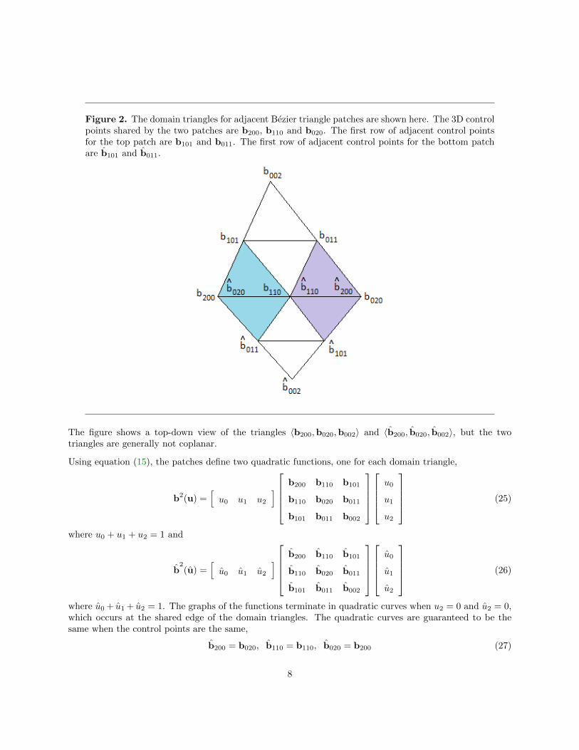
A comprehensive development of derivative continuity on the common boundary between two adjacenttriangular patches is provided in [3]. The main result is that derivatives up through order r of bn(u) dependonly on the shared row of control points on the boundary and the r rows of control points adjacent to thatboundary. I discuss only the cases relevant to the quadratic interpolation, namely, r = 0 and r = 1. Figure2 illustrates two adjacent triangle patches. The top patch has control points bI and the bottom patch hascontrol points bI .
7
Figure 2. The domain triangles for adjacent Bezier triangle patches are shown here. The 3D controlpoints shared by the two patches are b200, b110 and b020. The first row of adjacent control pointsfor the top patch are b101 and b011. The first row of adjacent control points for the bottom patchare b101 and b011.
The figure shows a top-down view of the triangles 〈b200,b020,b002〉 and 〈b200, b020, b002〉, but the twotriangles are generally not coplanar.
Using equation (15), the patches define two quadratic functions, one for each domain triangle,
b2(u) =[u0 u1 u2
]b200 b110 b101
b110 b020 b011
b101 b011 b002
u0
u1
u2
(25)
where u0 + u1 + u2 = 1 and
b2(u) =
[u0 u1 u2
]b200 b110 b101
b110 b020 b011
b101 b011 b002
u0
u1
u2
(26)
where u0 + u1 + u2 = 1. The graphs of the functions terminate in quadratic curves when u2 = 0 and u2 = 0,which occurs at the shared edge of the domain triangles. The quadratic curves are guaranteed to be thesame when the control points are the same,
b200 = b020, b110 = b110, b020 = b200 (27)
8
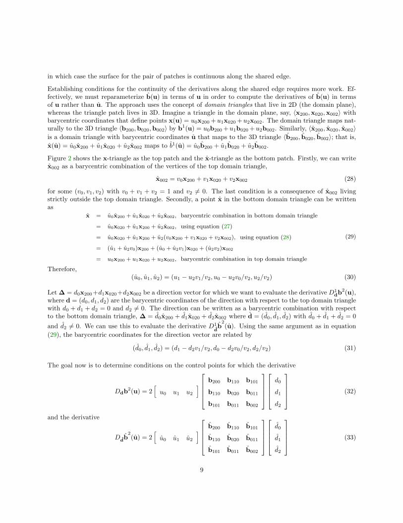
in which case the surface for the pair of patches is continuous along the shared edge.
Establishing conditions for the continuity of the derivatives along the shared edge requires more work. Ef-fectively, we must reparameterize b(u) in terms of u in order to compute the derivatives of b(u) in termsof u rather than u. The approach uses the concept of domain triangles that live in 2D (the domain plane),whereas the triangle patch lives in 3D. Imagine a triangle in the domain plane, say, 〈x200,x020,x002〉 withbarycentric coordinates that define points x(u) = u0x200 +u1x020 +u2x002. The domain triangle maps nat-urally to the 3D triangle 〈b200,b020,b002〉 by b1(u) = u0b200 +u1b020 +u2b002. Similarly, 〈x200, x020, x002〉is a domain triangle with barycentric coordinates u that maps to the 3D triangle 〈b200, b020, b002〉; that is,
Figure 2 shows the x-triangle as the top patch and the x-triangle as the bottom patch. Firstly, we can writex002 as a barycentric combination of the vertices of the top domain triangle,
x002 = v0x200 + v1x020 + v2x002 (28)
for some (v0, v1, v2) with v0 + v1 + v2 = 1 and v2 6= 0. The last condition is a consequence of x002 livingstrictly outside the top domain triangle. Secondly, a point x in the bottom domain triangle can be writtenas
x = u0x200 + u1x020 + u2x002, barycentric combination in bottom domain triangle
Let ∆ = d0x200+d1x020+d2x002 be a direction vector for which we want to evaluate the derivative D1db2(u),
where d = (d0, d1, d2) are the barycentric coordinates of the direction with respect to the top domain trianglewith d0 + d1 + d2 = 0 and d2 6= 0. The direction can be written as a barycentric combination with respectto the bottom domain triangle, ∆ = d0x200 + d1x020 + d2x002 where d = (d0, d1, d2) with d0 + d1 + d2 = 0
and d2 6= 0. We can use this to evaluate the derivative D1db2(u). Using the same argument as in equation
(29), the barycentric coordinates for the direction vector are related by
The goal now is to determine conditions on the control points for which the derivative
Ddb2(u) = 2[u0 u1 u2
]b200 b110 b101
b110 b020 b011
b101 b011 b002
d0
d1
d2
(32)
and the derivative
Ddb2(u) = 2
[u0 u1 u2
]b200 b110 b101
b110 b020 b011
b101 b011 b002
d0
d1
d2
(33)
9
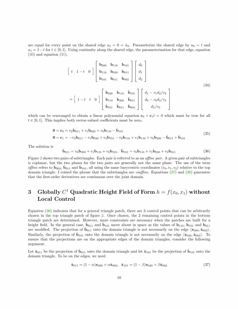
are equal for every point on the shared edge u2 = 0 = u2. Parameterize the shared edge by u0 = t andu1 = 1− t for t ∈ [0, 1]. Using continuity along the shared edge, the parameterization for that edge, equation(30) and equation (31),
[t 1− t 0
]b200 b110 b101
b110 b020 b011
b101 b011 b002
d0
d1
d2
=[
1− t t 0]
b020 b110 b101
b110 b200 b011
b101 b011 b002
d1 − v1d2/v2d0 − v0d2/v2
d2/v2
(34)
which can be rearranged to obtain a linear polynomial equation c0 + c1t = 0 which must be true for allt ∈ [0, 1]. This implies both vector-valued coefficients must be zero,
Figure 2 shows two pairs of subtriangles. Each pair is referred to as an affine pair. A given pair of subtrianglesis coplanar, but the two planes for the two pairs are generally not the same plane. The use of the termaffine refers to b002, b011 and b101, all using the same barycentric coordinates (v0, v1, v2) relative to the topdomain triangle. I coined the phrase that the subtriangles are coaffine. Equations (27) and (36) guaranteethat the first-order derivatives are continuous over the joint domain.
3 Globally C1 Quadratic Height Field of Form h = f(x0, x1) withoutLocal Control
Equation (36) indicates that for a general triangle patch, there are 3 control points that can be arbitrarilychosen in the top triangle patch of figure 2. Once chosen, the 2 remaining control points in the bottomtriangle patch are determined. However, more constraints are necessary when the patches are built for aheight field. In the general case, b011 and b101 move about in space as the values of b110, b101 and b011
are modified. The projection of b011 onto the domain triangle is not necessarily on the edge 〈x200, x002〉.Similarly, the projection of b101 onto the domain triangle is not necessarily on the edge 〈x020, x002〉. Toensure that the projections are on the appropriate edges of the domain triangles, consider the followingargument.
Let x011 be the projection of b011 onto the domain triangle and let x101 be the projection of b101 onto thedomain triangle. To be on the edges, we need
for some α ∈ (0, 1) and β ∈ (0, 1). Let the projections of bI onto the domain plane be xI . We require thatthe projections lie on the appropriate edges of the domain triangle; that is,
Subtracting the two equations,x110 − x101 = δ(x020 − x002) (41)
which says that the edges 〈x110,x101〉 and 〈x020,x002〉 are parallel. Therefore, the subtriangle 〈x200,x110,x101〉and the original triangle 〈x200,x020,x002〉 are similar triangles.
The construction can be applied to the other cases to show that
• The triangles 〈x200,x020,x002〉, 〈x200,x110,x101〉 and 〈x110,x020,x011〉 are similar.
• The triangles 〈x200, x020, x002〉, 〈x200, x110, x101〉 and 〈x110, x020, x011〉 are similar.
For derivative continuity of a height field formed by triangle patches, we need the aforementioned similarityof triangles in addition to the constraints of equations (27) and (36).
In the general case for two adjacent triangle patches, we can freely choose the 3 control points b110, b101
and b011, after which b101 and b011 are determined according to the construction presented here. In theheight-field case, we can freely choose only 1 control point, say, b110, after which b101, b011, b101 and b011are determined.
The degree of freedom in the height-field case is lost when a triangle in the mesh has at least 2 adjacenttriangles. Figure 3 illustrates the problem.
11
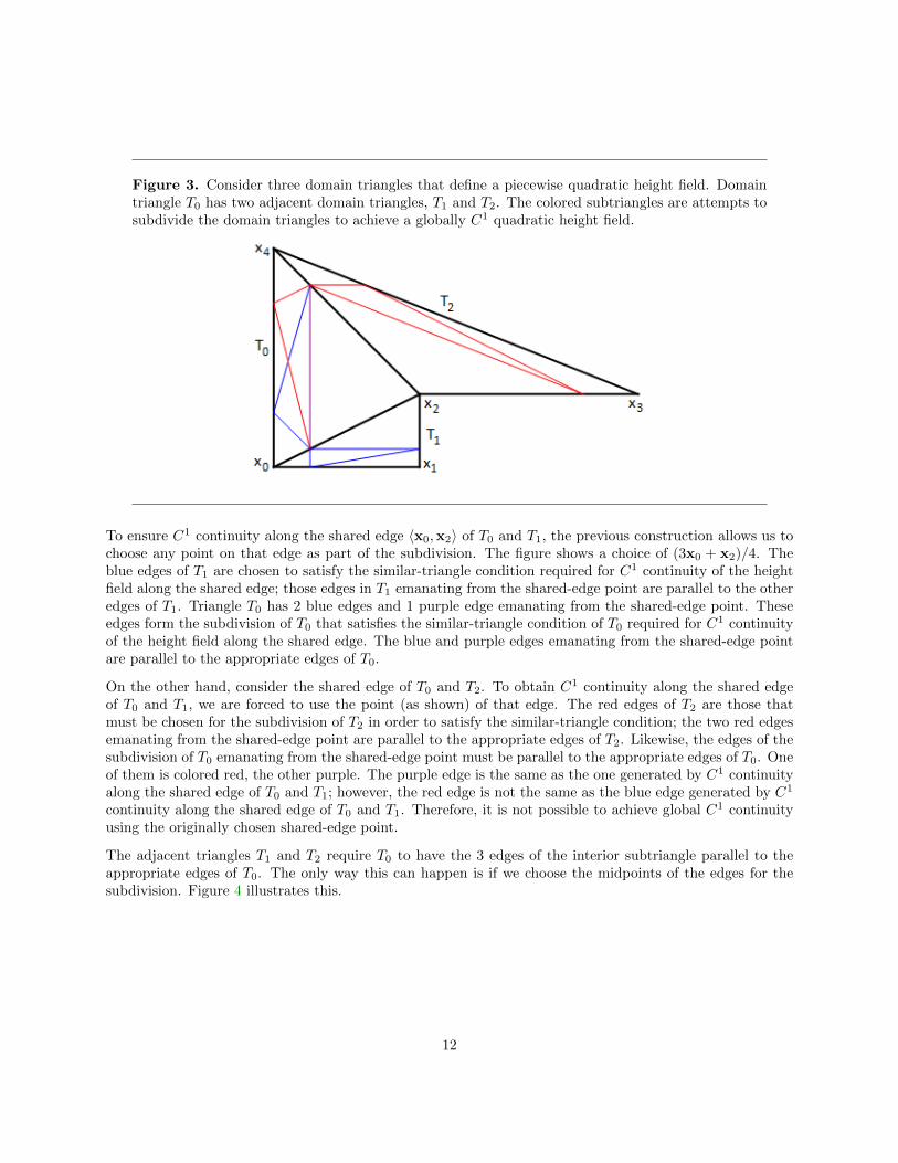
Figure 3. Consider three domain triangles that define a piecewise quadratic height field. Domaintriangle T0 has two adjacent domain triangles, T1 and T2. The colored subtriangles are attempts tosubdivide the domain triangles to achieve a globally C1 quadratic height field.
To ensure C1 continuity along the shared edge 〈x0,x2〉 of T0 and T1, the previous construction allows us tochoose any point on that edge as part of the subdivision. The figure shows a choice of (3x0 + x2)/4. Theblue edges of T1 are chosen to satisfy the similar-triangle condition required for C1 continuity of the heightfield along the shared edge; those edges in T1 emanating from the shared-edge point are parallel to the otheredges of T1. Triangle T0 has 2 blue edges and 1 purple edge emanating from the shared-edge point. Theseedges form the subdivision of T0 that satisfies the similar-triangle condition of T0 required for C1 continuityof the height field along the shared edge. The blue and purple edges emanating from the shared-edge pointare parallel to the appropriate edges of T0.
On the other hand, consider the shared edge of T0 and T2. To obtain C1 continuity along the shared edgeof T0 and T1, we are forced to use the point (as shown) of that edge. The red edges of T2 are those thatmust be chosen for the subdivision of T2 in order to satisfy the similar-triangle condition; the two red edgesemanating from the shared-edge point are parallel to the appropriate edges of T2. Likewise, the edges of thesubdivision of T0 emanating from the shared-edge point must be parallel to the appropriate edges of T0. Oneof them is colored red, the other purple. The purple edge is the same as the one generated by C1 continuityalong the shared edge of T0 and T1; however, the red edge is not the same as the blue edge generated by C1
continuity along the shared edge of T0 and T1. Therefore, it is not possible to achieve global C1 continuityusing the originally chosen shared-edge point.
The adjacent triangles T1 and T2 require T0 to have the 3 edges of the interior subtriangle parallel to theappropriate edges of T0. The only way this can happen is if we choose the midpoints of the edges for thesubdivision. Figure 4 illustrates this.
12
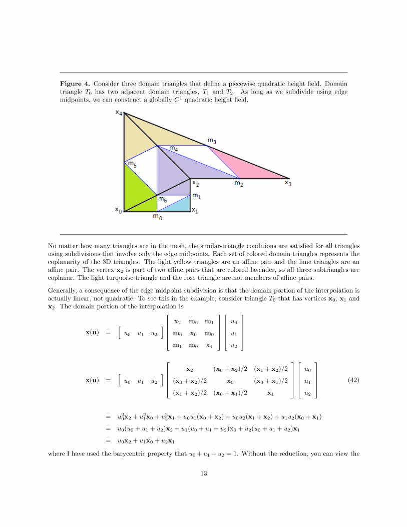
Figure 4. Consider three domain triangles that define a piecewise quadratic height field. Domaintriangle T0 has two adjacent domain triangles, T1 and T2. As long as we subdivide using edgemidpoints, we can construct a globally C1 quadratic height field.
No matter how many triangles are in the mesh, the similar-triangle conditions are satisfied for all trianglesusing subdivisions that involve only the edge midpoints. Each set of colored domain triangles represents thecoplanarity of the 3D triangles. The light yellow triangles are an affine pair and the lime triangles are anaffine pair. The vertex x2 is part of two affine pairs that are colored lavender, so all three subtriangles arecoplanar. The light turquoise triangle and the rose triangle are not members of affine pairs.
Generally, a consequence of the edge-midpoint subdivision is that the domain portion of the interpolation isactually linear, not quadratic. To see this in the example, consider triangle T0 that has vertices x0, x1 andx2. The domain portion of the interpolation is
where I have used the barycentric property that u0 + u1 + u2 = 1. Without the reduction, you can view the
13
quadratic polynomial representing the domain variables as degree elevation of the linear polynomial. Theheight portion of the interpolation is quadratic and, generally, not reducible to a linear polynomial unlessall the 3D control points are coplanar.
Let the known positions and heights in figure 4 be named (xi, fi) for 0 ≤ i ≤ 4. The midpoints are labeledmj for 0 ≤ j ≤ 6. The heights at the midpoint are named hi and are unknowns to be determined. Letthe normal vectors to the purported tangent planes to the surface at the (xi, fi) be named (Ni,−1), whereNi ∈ R2. The normals are not necessarily unit length vectors, so the components of Ni can be consideredto be the first-order partial derivatives of the height field; that is, Ni = ∇fi. The planes at the vertices arerepresented algebraically by z = Ni · (x− xi) + fi. The unknown heights are determined by
h0 = N0 · (m0 − x0) + f0 = N1 · (m0 − x1) + f1
h1 = N1 · (m1 − x1) + f1 = N2 · (m1 − x2) + f2
h2 = N2 · (m2 − x2) + f2 = N3 · (m2 − x3) + f3
h3 = N3 · (m3 − x3) + f3 = N4 · (m3 − x4) + f4
h4 = N4 · (m4 − x4) + f4 = N2 · (m4 − x2) + f2
h5 = N4 · (m5 − x4) + f4 = N0 · (m5 − x0) + f0
h6 = N0 · (m6 − x0) + f0 = N2 · (m6 − x2) + f2
(43)
These provide 7 linear equations in the 10 unknown components of Ni, so we expect to have 3 degrees offreedom for those components.
The degrees of freedom are better understood geometrically. Suppose we choose N0 arbitrarily, using up 2of the 3 degrees of freedom. The tangent plane at x0 is now known, which in turn determines the heights h0,h5 and h6 because the points (m0, h0), (m5, h5) and (m6, h6) are on that plane. Now consider the tangentplane at x4. We know that (x4, f4) and (m5, h5) are on that plane, which means that one of the componentsof N4 is determined. The other component is yet unknown, because the plane can rotate about the linecontaining the two known points on the plane. Choose that component (or choose a linear equation relatingthe two components), which uses the last of the degrees of freedom. The plane at x4 is known, which in turndetermines the heights h3 and h4 because the points (m3, h3) and (m4, h4) are on that plane.
The points (x2, f2), (m4, h4) and (m6, h6) are all known, which determines the tangent plane at x2. In turn,this plane determines h1 and h2 because the points (m1, h1) and (m2, h2) are on that plane. Finally, wenow know the points (m0, h0), (x1, f1) and (m1, h1), which determines the tangent plane at x1. And wenow know the points (m2, h2), (x3, f3) and (m3, h3), which determines the tangent plane at x3.
To illustrate using the triangles of figure 4, let (x0, f0) = ((0, 0), 0), (x1, f1) = ((2, 0), 3), (x2, f2) = ((2, 1), 4),(x3, f3) = ((5, 1), 1) and (x4, f4) = ((0, 3), 2). Choose N0 = (1, 1) and N1 = (α, β) where α+ β = 1. Figure5 shows the graph of the globally C1 quadratic height field satisfying the aforementioned conditions.
14
Figure 5. Two views of the graph of a C1 quadratic height field without local control. The domainof the height field is shown in figure 4.
4 Globally C1 Quadratic Height Field of Form h = f(x0, x1) withLocal Control
The example of the previous section is unappealing in that there are 3 degrees of freedom, forcing you tochoose that freedom by selecting a normal vector at one vertex and imposing an arbitrary condition in orderto determine the normals at the remaining vertices. More desirable is to have an algorithm that is symmetricin that each sample point has the same type of information. This can be accomplished by subdividing thetriangles that occur in the domain triangulation of the samples in order to obtain more degrees of freedom.Some derivative information is required, even in the example of the previous section, so our goal is to havea set of samples of the form (xi, fi,∇fi).
As a first attempt at subdivision, choose an interior point of a triangle and subdivide the triangle into 3subtriangles by connecting the interior point to the 3 vertices. Each subtriangle is itself subdivided into4 subtriangles using edge-midpoints for the subdivision. Figure 6 (a) shows the subdivision for a triangle〈x0,x1,x2〉 drawn using thick black lines. The interior point is c. The first level of subdivision is drawnusing blue lines. The mij are the midpoints of the edges of the original triangle. The pi are the midpointsof the edges on which they live. The second level of subdivision is drawn using red lines. The samplesare (xi, fi,∇fi) for 0 ≤ i ≤ 2. The tangent planes are therefore determined at the vertices of the originaltriangle. The colored regions indicate the subtriangles that are coplanar because of the coaffinity condition.
In figure 6 (a), the tangent plane at x0 determines the heights at m01 and m02, the tangent plane at x1
determines the heights at m01 and m12 and the tangent plane at x2 determines the heights at m12 and m02,all overconstrained problems.
In figure 6 (b), the problem is remedied by subdividing the original triangle into 6 subtriangles which aredrawn using blue lines. Each of the 6 subtriangles is further subdivided using midpoints of edges, and thesesubtriangles are drawn using red lines. As we will see, the heights at the subdivison points are properlyconstrained.
15
Figure 6. (a) An attempt at subdivision to introduce more degrees of freedom in fitting the originaltriangle with a globally C1 quadratic height field. The attempt fails because the heights hij at mij
are overconstrained. For example, the point (m01, h01) must be a point on the two independenttangent planes at x0 and x1. (b) An attempt at subdivision to introduce more degrees of freedom infitting the original triangle with a globally C1 quadratic height field. The attempt succeeds becausethe heights at the subdivision domain points are properly constrained.
(a) invalid subdivision (b) valid subdivision
The subdivision and height-fitting algorithm is described next, and is the material presented by Cendes andWong [2]. Choose an interior point c for the triangle. In barycentric coordinates,
c = u0x0 + u1x1 + u2x2 (44)
for ui ∈ (0, 1) with u0 + u1 + u2 = 1. Choose interior edge points e0, e1 and e2, which are not required tobe midpoints of the original triangle’s edges. In barycentric coordinates,
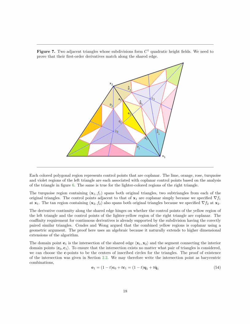
The previous equations determine the subdivision points and heights that lead to a C1 quadratic height field.However, we must now prove that two adjacent triangles, both subdivided accordingly, form a C1 quadraticheight field. Figure 7 shows two such triangles. The figure has labels only for the subdivision domain pointsthat affect influence the derivative continuity. We know the domain point equations for the left triangle. Forthe right triangle we have p1 = (x1 + c1)/2, p2 = (x2 + c2)/2 and q1 = (1− v1)p1 + v1p2. The heights atthose points are hp1
Figure 7. Two adjacent triangles whose subdivisions form C1 quadratic height fields. We need toprove that their first-order derivatives match along the shared edge.
Each colored polygonal region represents control points that are coplanar. The lime, orange, rose, turquoiseand violet regions of the left triangle are each associated with coplanar control points based on the analysisof the triangle in figure 6. The same is true for the lighter-colored regions of the right triangle.
The turquoise region containing (x1, f1) spans both original triangles, two subtriangles from each of theoriginal triangles. The control points adjacent to that of x1 are coplanar simply because we specified ∇f1at x1. The tan region containing (x2, f2) also spans both original triangles because we specified ∇f2 at x2.
The derivative continuity along the shared edge hinges on whether the control points of the yellow region ofthe left triangle and the control points of the lighter-yellow region of the right triangle are coplanar. Thecoaffinity requirement for continuous derivatives is already supported by the subdivision having the corectlypaired similar triangles. Cendes and Wong argued that the combined yellow regions is coplanar using ageometric argument. The proof here uses an algebraic because it naturally extends to higher dimensionalextensions of the algorithm.
The domain point e1 is the intersection of the shared edge 〈x1,x2〉 and the segment connecting the interiordomain points 〈c0, c1〉. To ensure that the intersection exists no matter what pair of triangles is considered,we can choose the c-points to be the centers of inscribed circles for the triangles. The proof of existenceof the intersection was given in Section 2.2. We may therefore write the intersection point as barycentriccombinations,
e1 = (1− t)c0 + tc1 = (1− t)q1 + tq1 (54)
18
for some t ∈ (0, 1). The last equality uses q1 = (c0 + e1)/2 and q1 = (c1 + e1)/2. The height at e1 is
which proves that the control points (e1, he1), (q1, hq1) and (q1, hq1
) are collinear. This fact together with
the coplanarity of {q1,a2,a3, e1} and the coplanarity of {q1,a2,a3, e1} imply that {q1,a2,a3, e1, q1} arecoplanar. In summary, the 4 subtriangles in the yellow-colored regions of figure 7 are coplanar which impliesthat the two quadratic Bezier triangle patches have continuous derivatives on the shared boundary.
5 The Algorithm for Graphs of f(x, y, z)
The Cendes-Wong algorithm may be extended to the interpolation of graphs of functions of three variables.
It is assumed that the 3D points have been tetrahedralized. Consider a tetrahedron whose vertices are Vi,0 ≤ i ≤ 3. Let C be the center of the inscribed sphere for the tetrahedron. Let Fijk be a point on the face
19
with vertices Vi, Vj , and Vk. If the face is shared with another tetrahedron, let Fijk be the intersection ofthat face and the line connecting the inscribed centers of the tetrahedra sharing that face. If the face is notshared, let Fijk be the average of the vertices for that face. Let Eij be the midpoint of the edge joiningvertices Vi and Vj where i < j. Such a consistent choice, when multiple tetrahedra share the same edge,allows the construction of the Bezier net without having to analyze neighbor relationships. However, if onlytwo tetrahedra share the same edge, then any interior edge point suffices.
The tetrahedron can be subdivided into 24 smaller tetrahedrons, each having four vertices consisting ofC, a vertex Vi, an edge point Eij , and a face point Fijk. Figure 8 shows a typical tetrahedron and onesubtetrahedron.
Figure 8. Subdivision of a tetrahedron.
Each face of a subtetrahedron is partitioned into four Bezier triangles by selecting the midpoints of each ofthe edges. Figure 9 shows the labeling of those midpoints.
20
Figure 9. Subdivision of a subtetrahedron.
The equations relating all the labeled points are given below.
Fijk = f0Vi + f1Vj + f2Vk; fi ≥ 0, f0 + f1 + f2 = 1 4 equations
Eij = (Vi + Vj)/2 6 equations
V Eij = (Vi + Eij)/2 12 equations
V Fijk = (Vi + Fijk)/2 12 equations
CVi = (C + Vi)/2 4 equations
CEij = (Eij + C)/2 6 equations
CFijk = (C + Fijk)/2 4 equations
EFijk = (Eij + Fijk)/2 12 equations
(60)
There are a total of 61 equations relating the points. The same number of equations relates the samplevalues at those points. Compare this to the 19 values in the 2-dimensional case.
It is also assumed that at each vertex a function value and gradient have been specified. At vertex Vi letthe function value be φVi
and let the gradient vector be ∇φVi. The remaining sample values will be denoted
φP where P is one of the points mentioned previously. To guarantee derivative continuity at a vertex, theBezier net about that vertex must be covolumetric. This is possible by choosing
φV Eij= φVi
+∇φVi· (V Eij − Vi)
φV Fijk= φVi
+∇φVi· (V Fijk − Vi)
φCVi = φVi +∇φVi · (C − Vi)
(61)
21
From these equations and the barycentric relationships, it follows that
φFijk= f0φV Fijk
+ f1φV Fjki+ f2φV Fkij
φC = c0φCV0+ c1φCV1
+ c2φCV2+ c3φCV3
φCFijk= f0φCVi
+ f1φCVj+ f2φCVk
(62)
To guarantee derivative continuity along the edges, we need
φEij= (φV Eij
+ φV Eji)/2 (63)
The 1/2 factor occurs because Eij was chosen as the midpoint between two vertices, so it is also the midpointbetween V Eij and V Eji. Also note that φEij
must depend only on function values at Vi and Vj since it ispossible for arbitrarily many tetrahedrons to share an edge. Any dependence of an edge value on a particulartetrahedron would invalidate the construction.
It is also necessary that the subtetrahedrons containing the edge between V Eij and V Eji are covolumetric.Define
∇φij =φV Eij
− φV Eji
|V Eij − V Eji|2(V Eij − V Eji) (64)
The remaining sample values are determined by
φCEij = φEij +∇φij · (C − Eij)
φEFijk= φEij
+∇φij · (EFijk − Eij)(65)
The argument of coaffinity is the same as in the 2D case: covolumetricity and midpoint subdivision implycoaffinity. However, this is more challenging to visualize since the covolumetricity refers to two 3-dimensionaltetrahedrons belonging to the same 3-dimensional hyperplane which lives in 4D.
6 The Algorithm for Surfaces
This section is a description of an extension of the Cendes-Wong algorithm to triangular meshes which arenot necessarily the graph of a function. If mesh is assumed to be sample from a parameterized surface(x(s, t), y(s, t), z(s, t)), the mesh vertices are of the form Vi = (xi, yi, zi; si, ti) where the vertex position is(xi, yi, zi) and the surface parameters (texture coordinates, so to speak) are (si, ti). Each component x(s, t),y(s, t) and z(s, t) is a height field of the surface parmemters. The Cendes-Wong algorithm can be applied toeach component separately to generate a globally C1 interpolated surface.
If surface parameters are not know at the mesh vertices, they can be generated using concepts found in [1].Of course, the topology of the mesh is important in selecting the parameterization algorithm.
References
[1] Mario Botsch, Leif Kobbelt, Mark Pauly, Pierre Alliez, and Bruno Levy. Polygon Mesh Processing. AKPeters Ltd., Natick, MA, 2010.
22
[2] Zoltan J. Cendes and Steven H. Wong. C1 quadratic interpolation over arbitrary point sets. IEEEComputer Graphics and Applications, 7(11):8–16, November 1987.
[3] Gerald Farin. Curves and Surfaces for Computer Aided Geometric Design: A Practical Guide. AcademicPress, Inc., San Diego, CA, 1990.
[4] Dave F. Watson. Computing the n-dimensional Delaunay tessellation with application to Voronoi poly-topes. The Computer Journal, 24(2):167–172, 1981.