Lent 2000 version of March 8, 2001 Richard Weber C11: STATISTICS Contents Aims of this course ............................ iv Schedules ................................. iv Recommended books ........................... iv Keywords ................................. v Notation .................................. vii 1 Parameter estimation 1 1.1 What is Statistics? ............................ 1 1.2 RVs with values in n or n ....................... 2 1.3 Some important random variables .................... 4 1.4 Independent and IID RVs ........................ 5 1.5 Indicating dependence on parameters .................. 5 1.6 The notion of a statistic ......................... 5 1.7 Unbiased estimators ........................... 6 1.8 Sums of independent RVs ........................ 6 1.9 More important random variables .................... 7 1.10 Laws of large numbers .......................... 7 1.11 The Central Limit Theorem ....................... 8 1.12 Poisson process of rate λ ......................... 8 2 Maximum likelihood estimation 9 2.1 Maximum likelihood estimation ..................... 9 2.2 Sufficient statistics ............................ 11 3 The Rao-Blackwell theorem 13 3.1 Mean squared error ............................ 13 3.2 The Rao-Blackwell theorem ....................... 14 3.3 Consistency and asymptotic efficiency * ................. 16 3.4 Maximum likelihood and decision-making ................ 16 4 Confidence intervals 17 4.1 Interval estimation ............................ 17 4.2 Opinion polls ............................... 18 4.3 Constructing confidence intervals .................... 19 4.4 A shortcoming of confidence intervals* ................. 20 i
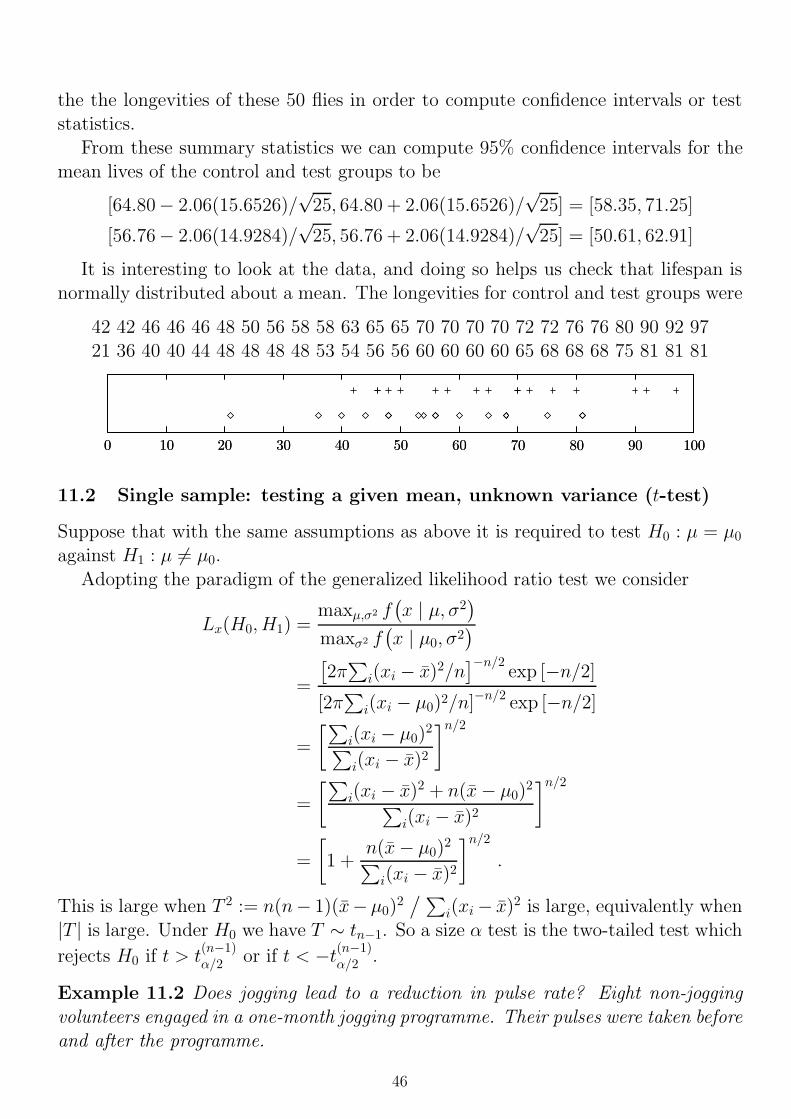
11 The t-test 4511.1 Confidence interval for the mean, unknown variance . . . . . . . . . . 4511.2 Single sample: testing a given mean, unknown variance (t-test) . . . . 4611.3 Two samples: testing equality of means, unknown common variance
The aim of this course is to aquaint you with the basics of mathematical statistics:the ideas of estimation, hypothesis testing and statistical modelling.
After studying this material you should be familiar with
1. the notation and keywords listed on the following pages;
2. the definitions, theorems, lemmas and proofs in these notes;
3. examples in notes and examples sheets that illustrate important issues concernedwith topics mentioned in the schedules.
Schedules
EstimationReview of distribution and density functions, parametric families, sufficiency, Rao-Blackwell theorem, factorization criterion, and examples; binomial, Poisson, gamma.Maximum likelihood estimation. Confidence intervals. Use of prior distributions andBayesian inference.
Hypothesis TestingSimple examples of hypothesis testing, null and alternative hypothesis, critical re-gion, size, power, type I and type II errors, Neyman-Pearson lemma. Significancelevel of outcome. Uniformly most powerful tests. Likelihood ratio, and the use oflikelihood ratio to construct test statistics for composite hypotheses. Generalizedlikelihood-ratio test. Goodness-of-fit and contingency tables.
Linear normal modelsThe χ2, t and F distribution, joint distribution of sample mean and variance, Stu-dent’s t-test, F -test for equality of two variances. One-way analysis of variance.
Linear regression and least squaresSimple examples, *Use of software*.
Recommended books
M. H. De Groot, Probability and Statistics, 2nd edition, Addison-Wesley, 1986.J. A. Rice, Mathematical Statistics and Data Analysis, 2nd edition, Duxbury Press,1994.G. Casella and J. O. Berger, Statistical Inference, Brooks Cole, 1990.D. A. Berry and B. W. Lindgren, Statistics, Theory and Methods, Brooks Cole, 1990(out of print).
iv
Keywords
absolute error loss, 24
acceptance region, 31
alternative hypothesis, 25
analysis of variance, 50
asymptotically efficient, 16
asymptotically unbiased, 12, 14
Bayesian inference, 21–24, 32
beta distribution, 7
between samples sum of squares, 51
biased, 10
binomial distribution, 4
bootstrap estimate, 64
Central Limit theorem, 8
chi-squared distribution, 33
χ2 test of homogeneity, 38
χ2 test of independence, 40
composite hypothesis, 26
confidence interval, 17–20, 31–32
consistent, 16
contingency table, 40
critical region, 26
decision-making, 2
degrees of freedom, 33, 38
discriminant analysis, 62
distribution function, 3
estimate, estimator, 6
expectation, 3
exponential distribution, 7
F -distribution, 49
factor analysis, 62
factorization criterion, 11
gamma distribution, 7
generalised likelihood ratio test, 33
geometric distribution, 7
goodness-of-fit, 26, 36
goodness-of-fit test, 37
hypothesis testing, 25
IID, 5
independent, 5
interval estimate, estimator, 17
Jacobian, 42
least squares estimators, 53
likelihood, 9, 27
likelihood ratio, 27
likelihood ratio test, 27
location parameter, 19
log-likelihood, 9
loss function, 24
maximum likelihood estimator(MLE), 9
mean squared error (MSE), 13
multinomial distribution, 36
Neyman–Pearson lemma, 27
non-central chi-squared, 50
nuisance parameter, 48
null hypothesis, 25
one-tailed test, 28
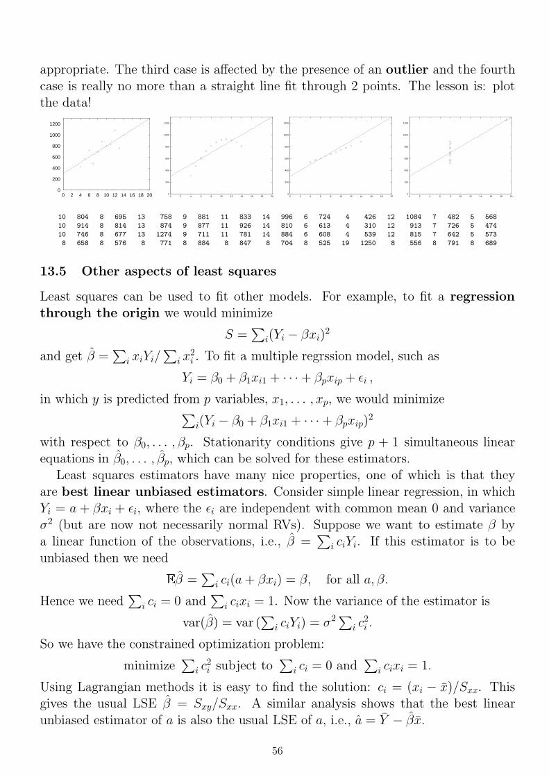
outlier, 56
p-value, 29
paired samples t-test, 47
parameter estimation, 1
parametric family, 5, 21, 25
Pearson chi-squared statistic, 37
point estimate, 17
Poisson distribution, 4
Poisson process, 8
v
posterior, 21
posterior mean, 24
posterior median, 24
power function, 29
predictive confidence interval, 58
principal components, 62
prior, 21
probability density function, 3
probability mass function, 3
quadratic error loss, 24
Rao–Blackwell theorem, 14
Rao–Blackwellization, 15
regression through the origin, 56
residual sum of squares, 57
RV, 2
sample correlation coefficient, 58
scale parameter, 19
significance level of a test, 26, 29
significance level of an observation,29
simple hypothesis, 26
simple linear regression model, 53
Simpson’s paradox, 41
size, 26
standard error, 45
standard normal, 4
standardized, 8
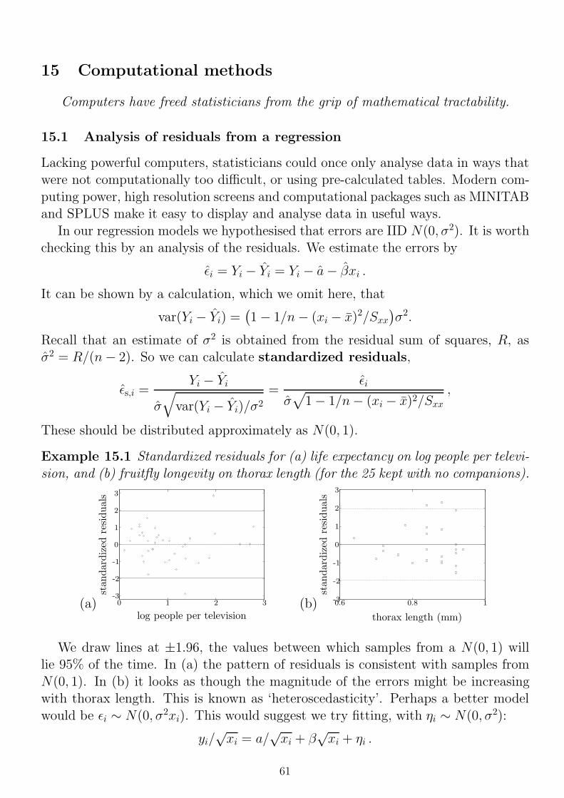
standardized residuals, 61
statistic, 5
strong law of large numbers, 8
sufficient statistic, 11
t-distribution, 18, 44
t-test, 46
two-tailed test, 28, 34
type I error, 26
type II error, 26
unbiased estimator, 6
uniform distribution, 4
uniformly most powerful, 30
variance, 3
weak law of large numbers, 8
within samples sum of squares, 51
vi
Notation
X a scalar or vector random variable, X = (X1, . . . , Xn)X ∼ X has the distribution . . .EX, var(X) mean and variance of Xµ, σ2 mean and variance as typically used for N(µ, σ2)RV, IID ‘random variable’, ‘independent and identically distributed’beta(m,n) beta distributionB(n, p) binomial distributionχ2n chi-squared distribution with n d.f.E(λ) exponential distributionFm,n F distribution with m and n d.f.gamma(n, λ) gamma distributionN(µ, σ2) normal (Gaussian) distributionP (λ) Poisson distributionU [a, b] uniform distributiontn Student’s t distribution with n d.f.Φ distribution function of N(0, 1)φ density function of N(0, 1)
zα, t(n)α , F
(m,n)α upper α points of N(0, 1), tn and Fm,n distributions
θ a parameter of a distribution
θ(X), θ(x) an estimator of θ, a estimate of θ.MLE ‘maximum likelihood estimator’FX(x | θ) distribution function of X depending on a parameter θfX(x | θ) density function of X depending on a parameter θfθ(x) density function depending on a parameter θfX |Y conditional density of X given Yp(θ | x) posterior density of θ given data xx1, . . . , xn n observed data valuesxi·, x·j, x··
∑j xij,
∑i xij and
∑ij xij
T (x) a statistic computed from x1, . . . , xn
vii
H0, H1 null and alternative hypothesesf0, f1 null and alternative density functionsLx(H0), Lx(H1) likelihoods of H0 and H1 given data xLx(H0, H1) likelihood ratio Lx(H1)/Lx(H0)
t(n)α , F
(m,n)α points to the right of which lie α100% of Tn and Fm,n
C critical region: reject H0 if T (x) ∈ C.W (θ) power function, W (θ) = P(X ∈ C | θ)α,β probabilities of Type I and Type II error
intercept and gradient of a regression line, Yi = α+ βwi + εioi, ei, δi observed and expected counts; δi = oi − eiX mean of X1, . . . , Xn
SXX , SY Y , SXY∑
(Xi − X)2,∑
(Yi − Y )2,∑
(Xi − X)(Yi − Y )s.e. ‘standard error’,
square root of an unbiased estimator of a variance.R residual sum of square in a regression models2 unbiased estimate of the variance, s2 = SXX/(n− 1).d(X) decision function, d(X) = a.L(θ, a) loss function when taking action a.R(θ, d) risk function, R(θ, d) = E [L(θ, d(X))].B(d) Bayes risk, E [R(θ, d)].
WWW site
There is a web page for this course, with copies of the lecture notes, examples sheets,corrections, past tripos questions, statistical tables and other additional material. Itcan be accessed as http://www.statslab.cam.ac.uk/~rrw1/stats/
viii
1 Parameter estimation
Statisticians do it when it counts.
1.1 What is Statistics?
Statistics is a collection of procedures and principles for gaining and processinginformation in order to make decisions when faced with uncertainty.
This course is concerned with “Mathematical Statistics”, i.e., mathematical ideasand tools that are used by statisticians to analyse data. We will study techniquesfor estimating parameters, fitting models, and testing hypotheses. However, as westudy these techniques we should not lose sight of the fact that a practicing statisti-cian needs more than simply a knowledge of mathematical techniques. The collectionand interpretation of data is a subtle art. It requires common sense. It can some-times raise philosophical questions. Although this course is primarily concerned withmathematical techniques, I will try — by means of examples and digressions — alsoto introduce you to some of the non-mathematical aspects of Statistics.
Statistics is concerned with data analysis : using data to make inferences. It isconcerned with questions like ‘what is this data telling me?’ and ‘what does thisdata suggest it reasonable to believe?’ Two of its principal concerns are parameterestimation and hypothesis testing.
Example 1.1 Suppose we wish to estimate the proportion p of students in Cambridgewho have not showered or bathed for over a day.
This is poses a number of questions. Who do we mean by students? Supposetime is limited and we can only interview 20 students in the street. Is it importantthat our survey be ‘random’? How can we ensure this? Will students we questionbe embarrassed to admit if they have not bathed? And even if we can get truthfulanswers, will we be happy with our estimate if that random sample turns out toinclude no women, or if it includes only computer scientists?
Suppose we find that 5 have not bathed for over a day. We might estimate p byp = 5/20 = 0.25. But how large an error might we expect p to have?
Many families of probability distributions depend on a small number of parame-ters; for example, the Poisson family depends on a single parameter λ and the Normalfamily on two parameters µ and σ. Unless the values of the parameters are knownin advance, they must be estimated from data. One major themes of mathematicalstatistics is the theory of parameter estimation and its use in fitting probabilitydistributions to data. A second major theme of Statistics is hypothesis testing.
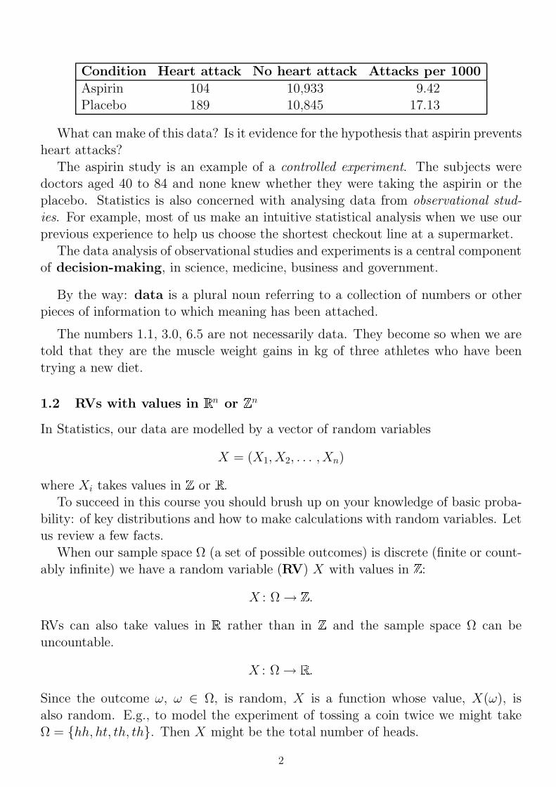
Example 1.2 A famous study investigated the effects upon heart attacks of takingan aspirin every other day. The results after 5 years were
1
Condition Heart attack No heart attack Attacks per 1000
Aspirin 104 10,933 9.42Placebo 189 10,845 17.13
What can make of this data? Is it evidence for the hypothesis that aspirin preventsheart attacks?
The aspirin study is an example of a controlled experiment. The subjects weredoctors aged 40 to 84 and none knew whether they were taking the aspirin or theplacebo. Statistics is also concerned with analysing data from observational stud-ies. For example, most of us make an intuitive statistical analysis when we use ourprevious experience to help us choose the shortest checkout line at a supermarket.
The data analysis of observational studies and experiments is a central componentof decision-making, in science, medicine, business and government.
By the way: data is a plural noun referring to a collection of numbers or otherpieces of information to which meaning has been attached.
The numbers 1.1, 3.0, 6.5 are not necessarily data. They become so when we aretold that they are the muscle weight gains in kg of three athletes who have beentrying a new diet.
1.2 RVs with values in Rn or Z
n
In Statistics, our data are modelled by a vector of random variables
X = (X1, X2, . . . , Xn)
where Xi takes values in Z or R .To succeed in this course you should brush up on your knowledge of basic proba-
bility: of key distributions and how to make calculations with random variables. Letus review a few facts.
When our sample space Ω (a set of possible outcomes) is discrete (finite or count-ably infinite) we have a random variable (RV) X with values in Z:
X : Ω→ Z.
RVs can also take values in R rather than in Z and the sample space Ω can beuncountable.
X : Ω→ R .
Since the outcome ω, ω ∈ Ω, is random, X is a function whose value, X(ω), isalso random. E.g., to model the experiment of tossing a coin twice we might takeΩ = hh, ht, th, th. Then X might be the total number of heads.
2
In both cases the distribution function FX of X is defined as:
FX(x) := P(X ≤ x) =∑
ω : X(ω)≤xP(ω).
In the discrete case the probability mass function (pmf) fX of X is
fX(k) := P(X = k), k ∈ Z.
So
P(X ∈ A) =∑x∈A
fX(x), A ⊆ Z.
In the continuous case we have the probability density function (pdf) fX of X.In all cases we shall meet, X will have a piecewise smooth pdf such that
P(X ∈ A) =
∫x∈A
fX(x) dx, for nice (measurable) subsets A ⊆ R .
Expectation of X: In the discrete case
E (X) :=∑ω∈Ω
X(ω)P(ω) =∑k∈Z
k P(X = k),
the first formula being the real definition. In the continuous case the calculation
E(X) =
∫ΩX(ω) P(dω)
needs measure theory. However,
fX(x) =d
dxFX(x) except perhaps for finitely many x.
Measure theory shows that for any nice function h on R ,
E h(X) =
∫R
h(x)fX(x) dx .
Variance of X: If E (X) = µ, then
var(X) = E (X − µ)2 = E (X2)− µ2.
3
1.3 Some important random variables
(a) We say that X has the binomial distribution B(n, p), and write X ∼ B(n, p),if
P(X = k) =
(nk
)pk(1− p)n−k if k ∈ 0, . . . , n,
0 otherwise.
Then E (X) = np, var(X) = np(1 − p). This is the distribution of the number ofsuccesses in n independent trials, each of which has probability of success p.
(b) We say that X has the Poisson distribution with parameter λ, and writeX ∼ P (λ), if
P(X = k) =
e−λλk/k! if k ∈ 0, 1, 2, . . .,0 otherwise.
Then E (X) = var(X) = λ. The Poisson is the limiting distribution of B(n, p) asn→∞ and p→ 0 with λ = np.
(c) We say that X is standard normal, and write X ∼ N(0, 1), if
fX(x) = ϕ(x) :=1√2π
exp(−x2/2), −∞ ≤ x ≤ ∞.
Then
FX(x) =
∫ x
−∞fX(y) dy = Φ(x) :=
∫ x
−∞ϕ(y) dy.
Then E (X) = 0, var(X) = 1. Φ and ϕ are standard notations.
(d) We say that X is Normal with mean µ and variance σ2 and write X ∼ N(µ, σ2)if
fX(x) =1
σ√
2πexp
(−(x− µ)2
2σ2
), −∞ ≤ x ≤ ∞.
Then E (X) = µ, var(X) = σ2.
(e) We say that X is uniform on [a, b], and write X ∼ U [a, b], if
fX(x) =1
b− a, x ∈ [a, b].
Then E (X) = 12(a+ b), var(X) = 1
12(b− a)2.
4
1.4 Independent and IID RVs
Random variables X1, . . . , Xn are called independent if for all x1, . . . , xn
IID stands for independent identically distributed. Thus if X1, X2, . . . , Xn areIID RVs, then they all have the same distribution function and hence the same meanand same variance.
We work with the probability mass function (pmf) of X in Zn or probability
density function (pdf) of X in Rn : In most cases, X1, . . . , Xn are independent, so
that if x = (x1, . . . , xn) ∈ Rn , then
fX(x) = fX1(x1) · · · fXn
(xn).
1.5 Indicating dependence on parameters
If X ∼ N(µ, σ2), then we indicate the dependence of the pdf of X on µ and σ2 bywriting it as
f(x | µ, σ2) =1
(2πσ2)1/2 exp
(−(x− µ)2
2σ2
)Or if X = (X1, . . . , Xn), where X1, . . . , Xn are IID N(µ, σ2), then we would have
f(x | µ, σ2) =1
(2πσ2)n/2exp
(−‖x− µ1‖2
2σ2
)where µ1 denotes the vector (µ, µ, . . . , µ)>.
In general, we write f(x | θ) to indicate that the pdf depends on a parameter θ.θ may be a vector of parameters. In the above θ = (µ, σ2)>. An alternative notationwe will sometimes employ is fθ(x).
The set of distributions with densities fθ(x), θ ∈ Θ, is called a parametricfamily. E.g.,, there is a parametric family of normal distributions, parameterisedby values of µ, σ2. Similarly, there is a parametric family of Poisson distributions,parameterised by values of λ.
1.6 The notion of a statistic
A statistic, T (x), is any function of the data. E.g., given the data x = (x1, . . . , xn),four possible statistics are
1
n(x1 + · · ·+ xn), max
ixi,
x1 + x3
xnlog x4, 1997 + 10 min
ixi.
Clearly, some statistics are more natural and useful than others. The first of thesewould be useful for estimating µ if the data are samples from a N(µ, 1) distribution.The second would be useful for estimating θ if the data are samples from U [0, θ].
5
1.7 Unbiased estimators
An estimator of a parameter θ is a function T = T (X) which we use to estimate θfrom an observation of X. T is said to be unbiased if
E (T ) = θ.
The expectation above is taken over X. Once the actual data x is observed, t = T (x)is the estimate of θ obtained via the estimator T .
Example 1.3 Suppose X1, . . . , Xn are IID B(1, p) and p is unknown. Consider theestimator for p given by p(X) = X =
∑iXi/n. Then p is unbiased, since
E p(X) = E
[1
n(X1 + · · ·+Xn)
]=
1
n(EX1 + · · ·+ EXn) =
1
nnp = p .
Another possible unbiased estimator for p is p = 13(X1 +2X2) (i.e., we ignore most
of the data.) It is also unbiased since
E p(X) = E
[1
3(X1 + 2X2)
]=
1
3(EX1 + 2EX2) =
1
3(p+ 2p) = p .
Intuitively, the first estimator seems preferable.
1.8 Sums of independent RVs
In the above calculations we have used the fact the expectation of a sum of randomvariables is the sum of their expectations. It is always true (even when X1, . . . , Xn
(a) We say that X is geometric with parameter p, if
P(X = k) =
p(1− p)k−1 if k ∈ 1, 2, . . .,0 otherwise.
Then E(X) = 1/p and var(X) = (1− p)/p2. X is the number of the toss on whichwe first observe a head if we toss a coin which shows heads with probability p.
(b) We say that X is exponential with rate λ, and write X ∼ E(λ), if
fX(x) =
λe−λx if x > 0,
0 otherwise.
Then E (X) = λ−1, var(X) = λ−2.The geometric and exponential distributions are discrete and continuous ana-
logues. They are the unique ‘memoryless’ distributions, in the sense that P(X ≥t + s | X ≥ t) = P(X ≥ s). The exponential is the distribution of the time betweensuccessive events of a Poisson process.
(c) We say that X is gamma(n, λ) if
fX(x) =
λnxn−1e−λx/(n− 1)! if x > 0,
0 otherwise.
X has the distribution of the sum of n IID RVs that have distribution E(λ). SoE(λ) = gamma(1, λ). E (X) = nλ−1 and var(X) = nλ−2.
This also makes sense for real n > 0 (and λ > 0), if we interpret (n− 1)! as Γ(n),where Γ(n) =
∫∞0 xn−1e−x dx.
(d) We say that X is beta(a, b) if
fX(x) =
1
B(a,b) xa−1(1− x)b−1 if 0 < x < 1,
0 otherwise.
Here B(a, b) = Γ(a)Γ(b)/Γ(a+ b). Then
E (X) =a
a+ b, var(X) =
ab
(a+ b+ 1)(a+ b)2 .
1.10 Laws of large numbers
Suppose X1, X2, . . . is a sequence of IID RVs, each having finite mean µ and varianceσ2. Let
Sn := X1 +X2 + · · ·+Xn, so that E (Sn) = nµ, var(Sn) = nσ2.
7
The weak law of large numbers is that for ε > 0,
P(|Sn/n− µ| > ε)→ 0, as n→∞ .
The strong law of large numbers is that
P(Sn/n→ µ) = 1 .
1.11 The Central Limit Theorem
Suppose X1, X2, . . . are as above. Define the standardized version S∗n of Sn as
S∗n =Sn − nµσ√n
, so that E (S∗n) = 0, var(S∗n) = 1.
Then for large n, S∗n is approximately standard Normal: for a < b,
limn→∞
P(a ≤ S∗n ≤ b) = Φ(b)− Φ(a) = limn→∞
P(nµ+ aσ
√n ≤ Sn ≤ nµ+ bσ
√n).
In particular, for large n,
P(|Sn − nµ| < 1.96σ√n) + 95%
since Φ(1.96) = 0.0975 and Φ(−1.96) = 0.025.
1.12 Poisson process of rate λ
The Poisson process is used to model a process of arrivals: of people to a supermarketcheckout, calls at telephone exchange, etc.
Arrivals happen at times
T1, T1 + T2, T1 + T2 + T3, . . .
where T1, T2, . . . are independent and each exponentially distributed with parameterλ. Numbers of arrivals in disjoint intervals are independent RVs, and the number ofarrivals in any interval of length t has the P (λt) distribution. The time
Sn = T1 + T2 + · · ·+ Tn
of the nth arrival has the gamma(n, λ) distribution, and 2λSn ∼ X 22n.
8
2 Maximum likelihood estimation
When it is not in our power to follow what is true, we oughtto follow what is most probable. (Descartes)
2.1 Maximum likelihood estimation
Suppose that the random variable X has probability density function f(x | θ). Giventhe observed value x of X, the likelihood of θ is defined by
lik(θ) = f(x | θ) .
Thus we are considering the density as a function of θ, for a fixed x. In the caseof multiple observations, i.e., when x = (x1, . . . , xn) is a vector of observed valuesof X1, . . . , Xn, we assume, unless otherwise stated, that X1, . . . , Xn are IID; in thiscase f(x1, . . . , xn | θ) is the product of the marginals,
lik(θ) = f(x1, . . . , xn | θ) =n∏i=1
f(xi | θ) .
It makes intuitive sense to estimate θ by whatever value gives greatest likelihoodto the observed data. Thus the maximum likelihood estimate θ(x) of θ is definedas the value of θ that maximizes the likelihood. Then θ(X) is called the maximumlikelihood estimator (MLE) of θ.
Of course, the maximum likelihood estimator need not exist, but in many examplesit does. In practice, we usually find the MLE by maximizing log f(x | θ), which isknown as the log-likelihood.
Examples 2.1
(a) Smarties are sweets which come in k equally frequent colours. Suppose we donot know k. We sequentially examine 3 Smarties and they are red, green, red. Thelikelihood of this data, x = the second Smartie differs in colour from the first but thethird Smartie matches the colour of the first, is
which equals 1/4, 2/9, 3/16 for k = 2, 3, 4, and continues to decrease for greater k.Hence the maximum likelihood estimate is k = 2.
Suppose a fourth Smartie is drawn and it is orange. Now
lik(k) = (k − 1)(k − 2)/k3 ,
9
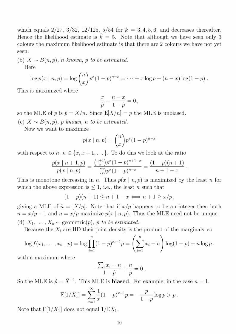
which equals 2/27, 3/32, 12/125, 5/54 for k = 3, 4, 5, 6, and decreases thereafter.Hence the likelihood estimate is k = 5. Note that although we have seen only 3colours the maximum likelihood estimate is that there are 2 colours we have not yetseen.
(b) X ∼ B(n, p), n known, p to be estimated.Here
log p(x | n, p) = log
(n
x
)px(1− p)n−x = · · ·+ x log p+ (n− x) log(1− p) .
This is maximized wherex
p− n− x
1− p = 0 ,
so the MLE of p is p = X/n. Since E [X/n] = p the MLE is unbiased.
(c) X ∼ B(n, p), p known, n to be estimated.Now we want to maximize
p(x | n, p) =
(n
x
)px(1− p)n−x
with respect to n, n ∈ x, x+ 1, . . . . To do this we look at the ratio
p(x | n+ 1, p)
p(x | n, p) =
(n+1x
)px(1− p)n+1−x(
nx
)px(1− p)n−x
=(1− p)(n+ 1)
n+ 1− x .
This is monotone decreasing in n. Thus p(x | n, p) is maximized by the least n forwhich the above expression is ≤ 1, i.e., the least n such that
(1− p)(n+ 1) ≤ n+ 1− x⇐⇒ n+ 1 ≥ x/p ,
giving a MLE of n = [X/p]. Note that if x/p happens to be an integer then bothn = x/p− 1 and n = x/p maximize p(x | n, p). Thus the MLE need not be unique.
(d) X1, . . . , Xn ∼ geometric(p), p to be estimated.Because the Xi are IID their joint density is the product of the marginals, so
log f(x1, . . . , xn | p) = logn∏i=1
(1− p)xi−1p =
(n∑i=1
xi − n)
log(1− p) + n log p .
with a maximum where
−∑
i xi − n1− p +
n
p= 0 .
So the MLE is p = X−1. This MLE is biased. For example, in the case n = 1,
E [1/X1] =∞∑x=1
1
x(1− p)x−1p = − p
1− p log p > p .
Note that E [1/X1] does not equal 1/EX1 .
10
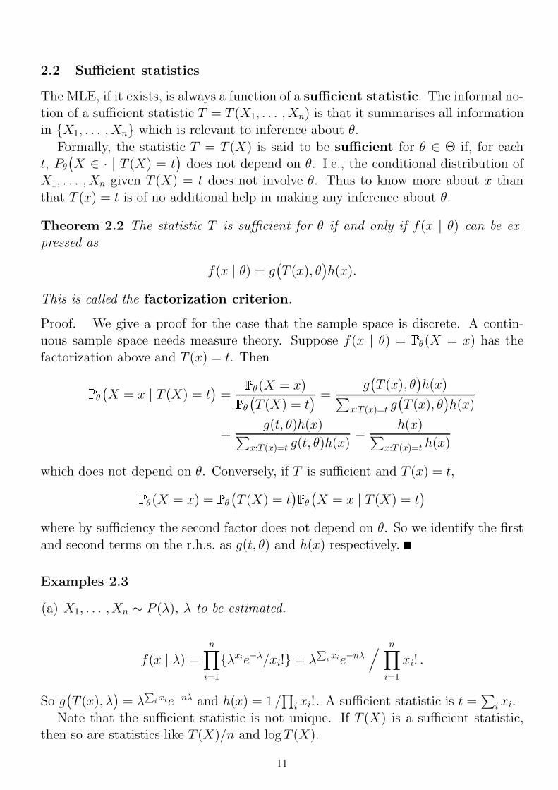
2.2 Sufficient statistics
The MLE, if it exists, is always a function of a sufficient statistic. The informal no-tion of a sufficient statistic T = T (X1, . . . , Xn) is that it summarises all informationin X1, . . . , Xn which is relevant to inference about θ.
Formally, the statistic T = T (X) is said to be sufficient for θ ∈ Θ if, for eacht, Pθ
(X ∈ · | T (X) = t
)does not depend on θ. I.e., the conditional distribution of
X1, . . . , Xn given T (X) = t does not involve θ. Thus to know more about x thanthat T (x) = t is of no additional help in making any inference about θ.
Theorem 2.2 The statistic T is sufficient for θ if and only if f(x | θ) can be ex-pressed as
f(x | θ) = g(T (x), θ
)h(x).
This is called the factorization criterion.
Proof. We give a proof for the case that the sample space is discrete. A contin-uous sample space needs measure theory. Suppose f(x | θ) = Pθ(X = x) has thefactorization above and T (x) = t. Then
Pθ
(X = x | T (X) = t
)=
Pθ(X = x)
Pθ
(T (X) = t
) =g(T (x), θ
)h(x)∑
x:T (x)=t g(T (x), θ
)h(x)
=g(t, θ)h(x)∑
x:T (x)=t g(t, θ)h(x)=
h(x)∑x:T (x)=t h(x)
which does not depend on θ. Conversely, if T is sufficient and T (x) = t,
Pθ(X = x) = Pθ
(T (X) = t
)Pθ
(X = x | T (X) = t
)where by sufficiency the second factor does not depend on θ. So we identify the firstand second terms on the r.h.s. as g(t, θ) and h(x) respectively.
Examples 2.3
(a) X1, . . . , Xn ∼ P (λ), λ to be estimated.
f(x | λ) =n∏i=1
λxie−λ/xi! = λ∑i xie−nλ
/ n∏i=1
xi! .
So g(T (x), λ
)= λ
∑i xie−nλ and h(x) = 1 /
∏i xi! . A sufficient statistic is t =
∑i xi.
Note that the sufficient statistic is not unique. If T (X) is a sufficient statistic,then so are statistics like T (X)/n and logT (X).
11
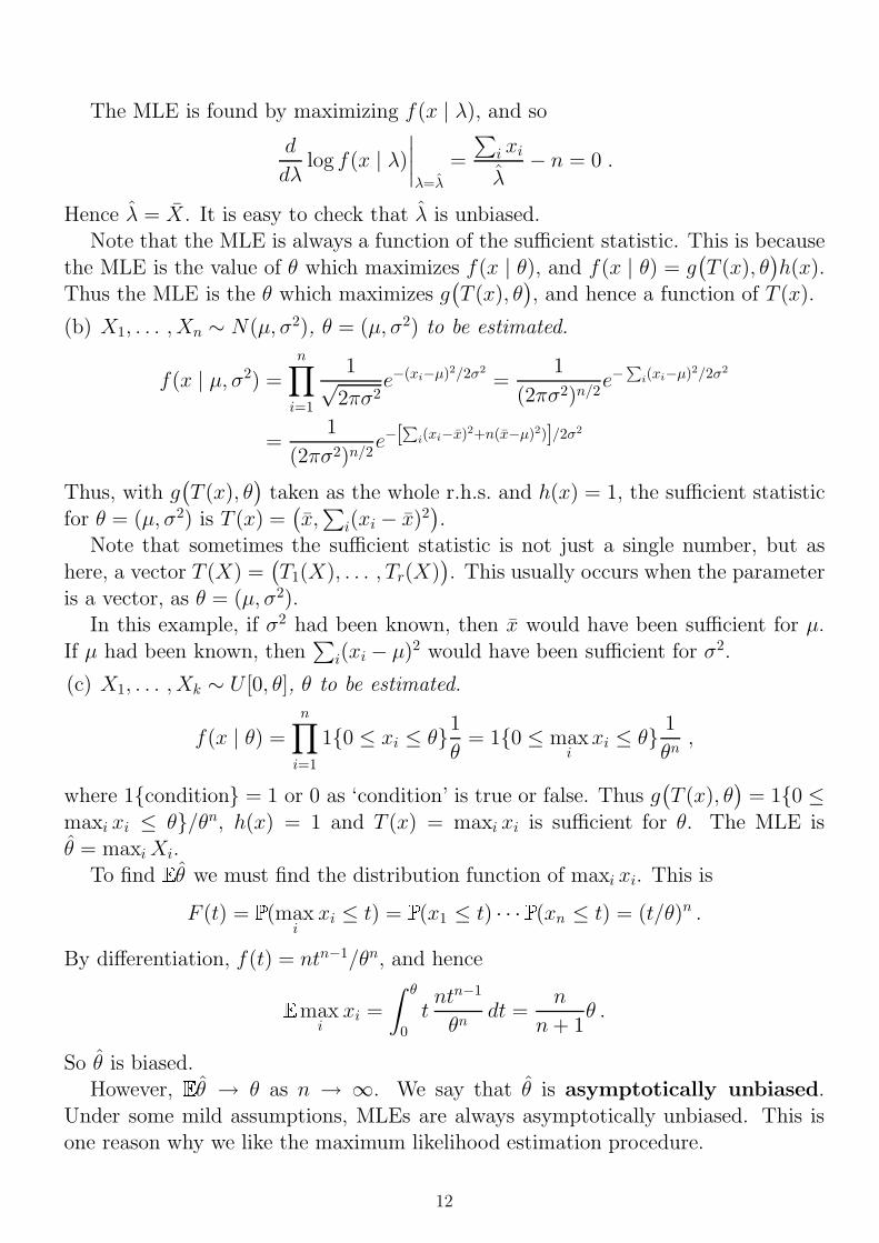
The MLE is found by maximizing f(x | λ), and so
d
dλlog f(x | λ)
∣∣∣∣λ=λ
=
∑i xi
λ− n = 0 .
Hence λ = X. It is easy to check that λ is unbiased.Note that the MLE is always a function of the sufficient statistic. This is because
the MLE is the value of θ which maximizes f(x | θ), and f(x | θ) = g(T (x), θ
)h(x).
Thus the MLE is the θ which maximizes g(T (x), θ
), and hence a function of T (x).
(b) X1, . . . , Xn ∼ N(µ, σ2), θ = (µ, σ2) to be estimated.
f(x | µ, σ2) =n∏i=1
1√2πσ2
e−(xi−µ)2/2σ2
=1
(2πσ2)n/2e−
∑i(xi−µ)2/2σ2
=1
(2πσ2)n/2e−[
∑i(xi−x)2+n(x−µ)2)]/2σ2
Thus, with g(T (x), θ
)taken as the whole r.h.s. and h(x) = 1, the sufficient statistic
for θ = (µ, σ2) is T (x) =(x,∑
i(xi − x)2).
Note that sometimes the sufficient statistic is not just a single number, but ashere, a vector T (X) =
(T1(X), . . . , Tr(X)
). This usually occurs when the parameter
is a vector, as θ = (µ, σ2).In this example, if σ2 had been known, then x would have been sufficient for µ.
If µ had been known, then∑
i(xi − µ)2 would have been sufficient for σ2.
(c) X1, . . . , Xk ∼ U [0, θ], θ to be estimated.
f(x | θ) =n∏i=1
10 ≤ xi ≤ θ1θ
= 10 ≤ maxixi ≤ θ 1
θn,
where 1condition = 1 or 0 as ‘condition’ is true or false. Thus g(T (x), θ
)= 10 ≤
maxi xi ≤ θ/θn, h(x) = 1 and T (x) = maxi xi is sufficient for θ. The MLE isθ = maxiXi.
To find E θ we must find the distribution function of maxi xi. This is
So θ is biased.However, E θ → θ as n → ∞. We say that θ is asymptotically unbiased.
Under some mild assumptions, MLEs are always asymptotically unbiased. This isone reason why we like the maximum likelihood estimation procedure.
12
3 The Rao-Blackwell theorem
Variance is what any two statisticians are at.
3.1 Mean squared error
A good estimator should take values close to the true value of the parameter it isattempting to estimate. If θ is an unbiased estimator of θ then E (θ − θ)2 is thevariance of θ. If θ is a biased estimator of θ then E (θ − θ)2 is no longer the varianceof θ, but it is still useful as a measure of the mean squared error (MSE) of θ.
Example 3.1 Consider the estimators in Example 1.3. Each is unbiased, so its MSEis just its variance.
var(p) = var
[1
n(X1 + · · ·+Xn)
]=
var(X1) · · ·+ var(Xn)
n2 =np(1− p)
n2 =p(1− p)
n
var(p) = var
[1
3(X1 + 2X2)
]=
var(X1) + 4 var(X2)
9=
5p(1− p)9
Not surprisingly, var(p) < var(p). In fact, var(p)/ var(p)→ 0, as n→∞.Note that p is the MLE of p. Another possible unbiased estimator would be
p∗ =1
12n(n+ 1)
(X1 + 2X2 + · · ·+ nXn)
with variance
var(p∗) =1[1
2n(n+ 1)]2(1 + 22 + · · ·+ n2)p(1− p) =
2(2n+ 1)
3n(n+ 1)p(1− p) .
Here var(p)/ var(p∗)→ 3/4.
The next example shows that neither a MLE or an unbiased estimator necessarilyminimizes the mean square error.
Example 3.2 Suppose X1, . . . , Xn ∼ N(µ, σ2), µ and σ2 unknown and to be esti-mated. To find the MLEs we consider
log f(x | µ, σ2) = logn∏i=1
1√2πσ2
e−(xi−µ)2/2σ2
= −n2
log(2πσ2)− 1
2σ2
n∑i=1
(xi − µ)2 .
This is maximized where ∂(log f)/∂µ = 0 and ∂(log f)/∂σ2 = 0. So
(1/σ2)n∑i=1
(xi − µ) = 0, and − n
2σ2 +1
2σ4
n∑i=1
(xi − µ)2 = 0,
13
and the MLEs are
µ = X =1
n
n∑i=1
Xi, σ2 =1
nSXX :=
1
n
n∑i=1
(Xi − X)2.
It is easy to check that µ is unbiased. As regards σ2 note that
E
[n∑i=1
(Xi − X)2
]= E
[n∑i=1
(Xi − µ+ µ− X)2
]= E
[n∑i=1
(Xi − µ)2
]− nE (µ − X)2
= nσ2 − n(σ2/n) = (n− 1)σ2
so σ2 is biased. An unbiased estimator is s2 = SXX/(n− 1).Let us consider an estimator of the form λSXX . Above we see SXX has mean
(n− 1)σ2 and later we will see that its variance is 2(n− 1)σ4. So
E[λSXX − σ2]2 =
[2(n− 1)σ4 + (n− 1)2σ4]λ2 − 2(n− 1)σ4λ+ σ4 .
This is minimized by λ = 1/(n+ 1). Thus the estimator which minimizes the meansquared error is SXX/(n + 1) and this is neither the MLE nor unbiased. Of coursethere is little difference between any of these estimators when n is large.
Note that E [σ2]→ σ2 as n→∞. So again the MLE is asymptotically unbiased.
3.2 The Rao-Blackwell theorem
The following theorem says that if we want an estimator with small MSE we canconfine our search to estimators which are functions of the sufficient statistic.
Theorem 3.3 (Rao-Blackwell Theorem) Let θ be an estimator of θ with E (θ2) <∞ for all θ. Suppose that T is sufficient for θ, and let θ∗ = E (θ | T ). Then for all θ,
E (θ∗ − θ)2 ≤ E (θ − θ)2.
The inequality is strict unless θ is a function of T .
Proof.
E [θ∗ − θ]2
= E
[E(θ | T
)− θ]2
= E
[E(θ − θ | T
)]2≤ E
[E((θ − θ)2 | T
)]= E (θ − θ)2
The outer expectation is being taken with respect to T . The inequality follows fromthe fact that for any RV, W , var(W ) = EW 2 − (EW )2 ≥ 0. We put W = (θ− θ | T )and note that there is equality only if var(W ) = 0, i.e., θ− θ can take just one valuefor each value of T , or in other words, θ is a function of T .
14
Note that if θ is unbiased then θ∗ is also unbiased, since
E θ∗ = E
[E (θ | T )
]= E θ = θ .
We now have a quantitative rationale for basing estimators on sufficient statistics:if an estimator is not a function of a sufficient statistic, then there is another estimatorwhich is a function of the sufficient statistic and which is at least as good, in thesense of mean squared error of estimation.
Examples 3.4
(a) X1, . . . , Xn ∼ P (λ), λ to be estimated.In Example 2.3 (a) we saw that a sufficient statistic is
∑i xi. Suppose we start
with the unbiased estimator λ = X1. Then ‘Rao–Blackwellization’ gives
λ∗ = E [X1 |∑
iXi = t] .
But ∑i
E[Xi |
∑iXi = t
]= E
[∑iXi |
∑iXi = t
]= t .
By the fact that X1, . . . , Xn are IID, every term within the sum on the l.h.s. mustbe the same, and hence equal to t/n. Thus we recover the estimator λ∗ = λ = X.
(b) X1, . . . , Xn ∼ P (λ), θ = e−λ to be estimated.Now θ = P(X1 = 0). So a simple unbiased estimator is θ = 1X1 = 0. Then
θ∗ = E
[1X1 = 0
∣∣∣ n∑i=1
Xi = t
]= P
(X1 = 0
∣∣∣ n∑i=1
Xi = t
)
= P
(X1 = 0;
n∑i=2
Xi = t
) /P
(n∑i=1
Xi = t
)
= e−λ((n− 1)λ)te−(n−1)λ
t!
/ (nλ)te−nλ
t!=
(n− 1
n
)tSince θ is unbiased, so is θ∗. As it should be, θ∗ is only a function of t. If you doRao-Blackwellization and you do not get just a function of t then you have made amistake.
(c) X1, . . . , Xn ∼ U [0, θ], θ to be estimated.In Example 2.3 (c) we saw that a sufficient statistic is maxi xi. Suppose we start
with the unbiased estimator θ = 2X1. Rao–Blackwellization gives
θ∗ = E [2X1 | maxiXi = t] = 2
(1
nt+
n− 1
n(t/2)
)=n+ 1
nt .
This is an unbiased estimator of θ. In the above calculation we use the idea thatX1 = maxiXi with probability 1/n, and if X1 is not the maximum then its expectedvalue is half the maximum. Note that the MLE θ = maxiXi is biased.
15
3.3 Consistency and asymptotic efficiency∗
Two further properties of maximum likelihood estimators are consistency and asymp-totic efficiency. Suppose θ is the MLE of θ.
To say that θ is consistent means that
P(|θ − θ| > ε)→ 0 as n→∞ .
In Example 3.1 this is just the weak law of large numbers:
P
(∣∣∣∣X1 + · · ·+Xn
n− p∣∣∣∣ > ε
)→ 0 .
It can be shown that var(θ) ≥ 1/nI(θ) for any unbiased estimate θ, where 1/nI(θ)is called the Cramer-Rao lower bound. To say that θ is asymptotically efficientmeans that
limn→∞
var(θ)/[1/nI(θ)] = 1 .
The MLE is asymptotically efficient and so asymptotically of minimum variance.
3.4 Maximum likelihood and decision-making
We have seen that the MLE is a function of the sufficient statistic, asymptoticallyunbiased, consistent and asymptotically efficient. These are nice properties. Butconsider the following example.
Example 3.5 You and a friend have agreed to meet sometime just after 12 noon.You have arrived at noon, have waited 5 minutes and your friend has not shownup. You believe that either your friend will arrive at X minutes past 12, where youbelieve X is exponentially distributed with an unknown parameter λ, λ > 0, or thatshe has completely forgotten and will not show up at all. We can associate the laterevent with the parameter value λ = 0. Then
P(data | λ) = P(you wait at least 5 minutes | λ) =
∫ ∞5
λe−λt dt = e−5λ .
Thus the maximum likelihood estimator for λ is λ = 0. If you base your decision asto whether or not you should wait a bit longer only upon the maximum likelihoodestimator of λ, then you will estimate that your friend will never arrive and decidenot to wait. This argument holds even if you have only waited 1 second.
The above analysis is unsatisfactory because we have not modelled the costs ofeither waiting in vain, or deciding not to wait but then having the friend turn up.
16
4 Confidence intervals
Statisticians do it with 95% confidence.
4.1 Interval estimation
Let a(X) and b(X) be two statistics satisfying a(X) ≤ b(X) for all X. Suppose thaton seeing the data X = x we make the inference a(x) ≤ θ ≤ b(x). Here [a(x), b(x)]is called an interval estimate and [a(X), b(X)] is called an interval estimator.
Previous lectures were concerned with making a point estimate for θ. Now weare being less precise. By giving up precision in our assertion about the value of θwe gain confidence that our assertion is correct. Suppose
Pθ
(a(X) ≤ θ ≤ b(X)
)= γ,
where γ does not depend on θ. Then the random interval[a(X), b(X)
]is called a
100γ% confidence interval for θ. Typically γ is 0.95 or 0.99, so that the probabilitythe interval contains θ is close to 1.
Given data x, we would call [a(x), b(x)] a ‘100γ% confidence interval for θ’. Noticehowever, that θ is fixed, and therefore the interval either does or does not containthe true θ. However, if we repeat the procedure of sampling and constructing a aconfidence interval many times, then our confidence interval will contain the true θ100γ% of the time. The point to understand here is that it is the endpoints of theconfidence interval that are random variables, not the parameter θ.
Examples 4.1
(a) If X1, . . . , Xn ∼ N(µ, σ2) independently, with µ unknown and σ2 known, then
X ∼ N(µ, σ2/n) and hence√n(X − µ)/σ ∼ N(0, 1) .
So if ξ and η are such that P(ξ ≤ N(0, 1) ≤ η) = γ, we have
P(µ,σ2)
(ξ ≤√n(X − µ)
σ≤ η
)= γ ,
which can be rewritten as
P(µ,σ2)
(X − ησ√
n≤ µ ≤ X − ξσ√
n
).
Note that the choice of ξ and η is not unique. However, it is natural to try to makethe length of the confidence interval as small as possible, so the symmetry of thenormal distribution implies that we should take ξ and η symmetric about 0.
17
Hence for a 95% confidence interval we would take −ξ = η = 1.96, as Φ(1.96) =0.975. The 95% confidence interval is[
X − 1.96σ√n
, X +1.96σ√
n
]For a 99% confidence interval, 1.96 would be replaced by 2.58, as Φ(2.58) = 0.995.
(b) If X1, . . . , Xn ∼ N(µ, σ2) independently, with µ and σ2 both unknown, then
√n(X − µ)√SXX/(n− 1)
∼ tn−1,
where tn−1 denotes the ‘Student’s t-distribution on n−1 degrees of freedom’ whichwill be studied later. So if ξ and η are such that P(ξ ≤ tn−1 ≤ η) = γ, we have
P(µ,σ2)
(ξ ≤
√n(X − µ)√
SXX/(n− 1)≤ η
)= γ,
which can be rewritten as
P(µ,σ2)
(X − η
√SXX/n(n− 1) ≤ µ ≤ X − ξ
√SXX/n(n− 1)
)= γ.
Again the choice of ξ and η is not unique, but it is natural to try to make the lengthof the confidence interval as small as possible. The symmetry of the t-distributionimplies that we should choose ξ and η symmetrically about 0.
4.2 Opinion polls
Opinion polls are typically quoted as being accurate to ±3%. What does this meanand how many people must be polled to attain this accuracy?
Suppose we are trying to estimate p, the proportion of people who support theLabour party amongst a very large population. We interview n people and estimatep from p = 1
n(X1 + · · · + Xn), where Xi = 1 if the ith person supports Labour andXi = 0 otherwise. Then
E p = p and var p =p(1− p)
n≤ 1
4n,
where the inequality follows from the fact that p(1− p) is maximized by p = 12 .
Let us approximate the distribution of p(X) by N(p, p(1 − p)/n
). This is very
good for n more than about 20. Then we have that approximately
(p− p)/√p(1− p)/n ∼ N(0, 1).
18
So
P(p − 0.03 ≤ p ≤ p+ 0.03)
= P
(− 0.03√
p(1− p)/n≤ p− p√
p(1− p)/n≤ 0.03√
p(1− p)/n
)≈ Φ
(0.03
√n/p(1− p)
)− Φ
(−0.03
√n/p(1− p)
)≥ Φ(0.03
√4n)− Φ(−0.03
√4n)
For this to be at least 0.95, we need 0.03√
4n ≥ 1.96, or n ≥ 1068.
Opinion polls typically use a sample size of about 1,100.
Example 4.2 U.S. News and World Report (Dec 19, 1994) reported on a telephonesurvey of 1,000 Americans, in which 59% said they believed the world would cometo an end, and of these 33% believed it would happen within a few years or decades.
Let us find a confidence interval for the proportion of Americans who believe theend of the world in imminent. Firstly, p = 0.59(0.33) = 0.195. The variance ofp is p(1 − p)/590 which we estimate by (0.195)(0.805)/590 = 0.000266. Thus anapproximate 95% confidence interval is 0.195±
√0.00266(1.96), or [0.163, 0.226].
Note that this is only approximately a 95% confidence interval. We have used thenormal approximation, and we have approximated p(1 − p) by p(1 − p). These areboth good approximations and this is therefore a very commonly used analysis.
Sampling from a small population*
For small populations the formula for the variance of p depends on the total popula-tion size N . E.g., if we are trying to estimate the proportion p of N = 200 studentsin a lecture who support the Labour party and we take n = 200, so we sample themall, then clearly var(p) = 0. If n = 190 the variance will be close to 0. In fact,
var(p) =
(N − nN − 1
)p(1− p)
n.
4.3 Constructing confidence intervals
The technique we have used in these examples is based upon finding some statisticwhose distribution does not depend on the unknown parameter θ. This can be donewhen θ is a location parameter or scale parameter. In section 4.1 µ is an exampleof a location parameter and σ is an example of a scale parameter. We saw that thedistribution of
√n(X − µ)/σ does not depend on µ or σ.
In the following example we consider a scale parameter.
19
Example 4.3 Suppose that X1, . . . , Xn are IID E(θ). Then
f(x | θ) =n∏i=1
θe−θxi = θne−θ∑i xi
so T (X) =∑
iXi is sufficient for θ. Also, T ∼ gamma(n, θ) with pdf
fT (t) = θntn−1e−θt/(n− 1)!, t > 0.
Consider S = 2θT . Now P(S ≤ s) = P(T ≤ s/2θ), so by differentiation with respectto s, we find the density of S to be
fS(s) = fT (s/2θ)1
2θ=θn(s/2θ)n−1e−θ(s/2θ)
(n− 1)!
1
2θ=sn−1(1/2)ne−s/2
(n− 1)!, s > 0 .
So S = 2θT ∼ gamma(n, 1
2
)≡ χ2
2n.Suppose we want a 95% confidence interval for the mean, 1/θ. We can write
For example, if n = 10 we refer to tables for the χ220 distribution and pick ξ = 34.17
and η = 9.59, so that F20(ξ) = 0.975, F20(η) = 0.025 and F20(ξ) − F20(η) = 0.95.Then a 95% confidence interval for 1/θ is
[2t/34.17 , 2t/9.59 ] .
Along the same lines, a confidence interval for σ can be constructed in the cir-cumstances of Example 4.1 (b) by using fact that SXX/σ
2 ∼ χ2n−1. E.g., if n = 21 a
95% confidence interval would be[√Sxx/34.17 ,
√Sxx/9.59
].
4.4 A shortcoming of confidence intervals*
Confidence intervals are widely used, e..g, in reporting the results of surveys andmedical experiments. However, the procedure has the problem that it sometimesfails to make the best interpretation of the data.
Example 4.4 Suppose X1, X2 are two IID samples from U(θ − 1
2, θ + 12
). Then
P(minixi ≤ θ ≤ max
ixi) = P(X1 ≤ θ ≤ X2) + P(X2 ≤ θ ≤ X1) =
1
2
1
2+
1
2
1
2=
1
2.
So (mini xi,maxi xi) is a 50% confidence interval for θ.But suppose the data is x = (7.4, 8.0). Then we know θ > 8.0 − 0.5 = 7.5 and
θ < 7.4 + 0.5 = 7.9. Thus with certainty, θ ∈ (7.5, 7.9) ⊂ (7.4, 8.0), so we can be100% certain, not 50% certain, that our confidence interval has captured θ. Thishappens whenever maxi xi −mini xi >
12.
20
5 Bayesian estimation
Bayesians probably do it.
5.1 Prior and posterior distributions
Bayesian statistics, (named after the Rev. Thomas Bayes, an amateur 18th centurymathematician), represents a different approach to statistical inference. Data are stillassumed to come from a distribution belonging to a known parametric family. How-ever, whereas classical statistics considers the parameters to be fixed but unknown,the Bayesian approach treats them as random variables in their own right. Priorbeliefs about θ are represented by the prior distribution, with a prior probabilitydensity (or mass) function, p(θ). The posterior distribution has posterior density(or mass) function, p(θ | x1, . . . , xn), and captures our beliefs about θ after they havebeen modified in the light of the observed data.
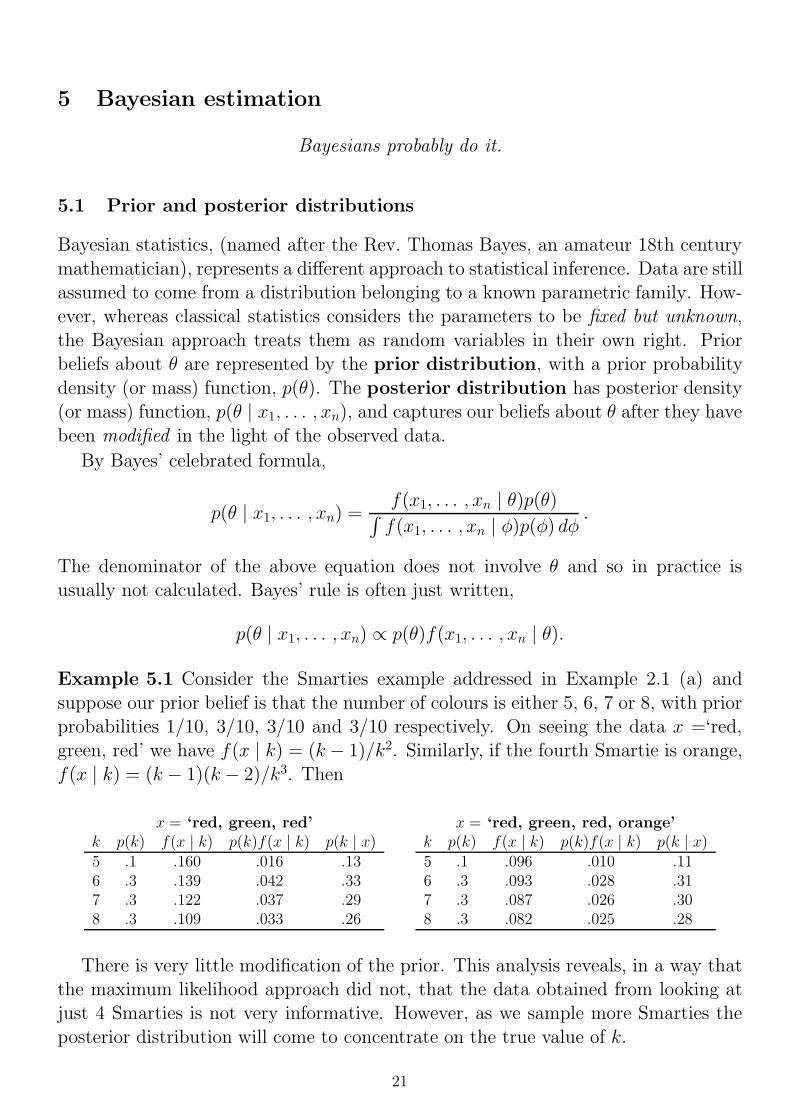
Example 5.1 Consider the Smarties example addressed in Example 2.1 (a) andsuppose our prior belief is that the number of colours is either 5, 6, 7 or 8, with priorprobabilities 1/10, 3/10, 3/10 and 3/10 respectively. On seeing the data x =‘red,green, red’ we have f(x | k) = (k − 1)/k2. Similarly, if the fourth Smartie is orange,f(x | k) = (k − 1)(k − 2)/k3. Then
There is very little modification of the prior. This analysis reveals, in a way thatthe maximum likelihood approach did not, that the data obtained from looking atjust 4 Smarties is not very informative. However, as we sample more Smarties theposterior distribution will come to concentrate on the true value of k.
21
5.2 Conditional pdfs
The discrete case
Thus Bayesians statistics relies on calculation of conditional distributions. For twoevents A and B (measurable subsets of the sample space) with P(B) 6= 0, we define
P(A | B) := P(A ∩ B)/P(B).
We can harmlessly agree to define P(A | B) := 0 if P(B) = 0.If X and Y are RVs with values in Z, and if fX,Y is their joint pmf:
P(X = x;Y = y) = fX,Y (x, y),
then we define
fX |Y (x | y) := P(X = x | Y = y) =P(X = x;Y = y)
P(Y = y)=fX,Y (x, y)
fY (y)
if fY (y) 6= 0. We can safely define fX |Y (x | y) := 0 if fY (y) = 0. Of course,
fY (y) = P(Y = y) =∑x
P(X = x;Y = y) =∑x
fX,Y (x, y).
Example 5.2 Suppose that X and R are independent RVs, where X is Poisson withparameter λ and R is Poisson with parameter µ. Let Y = X +R.
Then
fX |Y (x | y) =λxe−λ
x!
µy−xe−µ
(y − x)!
/ ∑x,r:x+r=y
λxe−λ
x!
µre−µ
r!
=y!
x!(y − x)!λxµ(y−x)
/ ∑x,r:x+r=y
y!
x!r!λxµr
=
(y
x
)(λ
λ+ µ
)x( µ
λ+ µ
)y−x.
Hence (X | Y = y) ∼ B(y, p), where p = λ/(λ+ µ).
The continuous case
Let Z = (X, Y ) be a RV with values in Rm+n, X having values in R
m and Y valuesin R
n . Assume that Z has nice pdf fZ(z) and write
fZ(z) = fX,Y (x, y), (z = (x, y), x ∈ Rm , y ∈ Rn).
Then the pdf of Y is given by
fY (y) =
∫Rm
fX,Y (x, y) dx.
22
We define fX |Y , the conditional pdf of X given Y , by
fX |Y (x | y) :=
fX,Y (x, y)/fY (y) if fY (y) 6= 0,
0 if fY (y) = 0.
The intuitive idea is: P(X ∈ dx | Y ∈ dy) = P(X ∈ dx;Y ∈ dy)/P(Y ∈ dy).
Examples 5.3
(a) A biased coin is tossed n times. Let xi be 1 or 0 as the ith toss is or is not ahead. Suppose we have no idea how biased the coin is, so we place a uniform priordistribution on θ, to give a so-called ‘noninformative prior’ of
p(θ) = 1, 0 ≤ θ ≤ 1 .
Let t be the number of heads. Then the posterior distribution of θ is
p(θ | x1, . . . , xn) = θt(1− θ)n−t × 1
/∫ 1
0φt(1− φ)n−t × 1 dφ .
We would usually not bother with the denominator and just write
p(θ | x) ∝ θt(1− θ)n−t .
By inspection we recognise that if the appropriate constant of of proportionalityis inserted on the r.h.s. then we have the density of beta(t+ 1, n− t + 1), so this isthe posterior distribution of θ given x.
(b) Suppose X1, . . . , Xn ∼ N(µ, 1), p(µ) ∼ N(0, τ−2) for known τ−2. Then
p(µ | x1, . . . , xn) ∝ exp
−1
2
(n∑i=1
(xi − µ)2 + µ2τ 2
)
∝ exp
−1
2(n+ τ 2)
(µ−
∑xi
n+ τ 2
)2
µ | x1, . . . , xn ∼ N
( ∑xi
n+ τ 2 ,1
n+ τ 2
)Note that as τ → 0 the prior distribution becomes less informative.
(c) Suppose X1, . . . , Xn ∼ IID E(λ), and the prior for λ is given by λ ∼ E(µ), forfixed and known µ. Then
p(λ | x1, . . . , xn) ∝ µe−λµ∏i
λe−λxi = λne−λ(µ+∑ni=1 xi) ,
i.e., gamma(n+ 1, µ+∑xi).
23
5.3 Estimation within Bayesian statistics
The Bayesian approach to the parameter estimation problem is to use a loss func-tion L(θ, a) to measure the loss incurred by estimating the value of a parameter tobe a when its true value is θ. Then θ is chosen to minimize E [L(θ, θ)], where thisexpectation is taken over θ with respect to the posterior distribution p(θ | x).
Loss functions for quadratic and absolute error loss
(a) L(θ, a) = (a− θ)2 is the quadratic error loss function.
E [L(θ, a)] =
∫L(θ, a)p(θ | x1, . . . , xn) dθ =
∫(a− θ)2p(θ | x1, . . . , xn) dθ .
Differentiating with respect to a we get
2
∫(a− θ)p(θ | x1, . . . , xn) dθ = 0 =⇒ a =
∫θp(θ | x1, . . . , xn) dθ .
Therefore quadratic error loss is minimized by taking θ to be the posterior mean.
(b) L(θ, a) = |a− θ| is the absolute error loss function.
E [L(θ, a)] =
∫L(θ, a)p(θ | x1, . . . , xn) dθ
=
∫ a
θ=−∞(a− θ)p(θ | x1, . . . , xn) dθ +
∫ ∞a
(θ − a)p(θ | x1, . . . , xn) dθ .
Differentiating with respect to a we find that the minimum is where∫ a
−∞p(θ | x1, . . . , xn) dθ −
∫ ∞a
p(θ | x1, . . . , xn) dθ = 0 .
The minimum is achieved when both integrals are equal to 12, i.e., by taking θ to be
the posterior median.
Example 5.4 Let X1, . . . , Xn ∼ P (λ), λ ∼ E(1) so that p(λ) = e−λ, λ ≥ 0.The posterior distribution is
p(λ | x1, . . . , xn) = e−λn∏i=1
e−λλxi
xi!∝ e−λ(n+1)λ
∑xi ,
i.e., gamma(∑
xi + 1, (n+ 1)). So under quadratic error loss,
θ = posterior mean =
∑ni=1 xi + 1
n+ 1.
Under absolute error loss, θ solves∫ θ
0
e−λ(n+1)λ∑xi(n+ 1)
∑xi+1
(∑xi)!
dλ =1
2.
24
6 Hypothesis testing
Statistics is the only profession which demands the right to make mistakes 5 percent of the time – Thomas Huxley.
6.1 The Neyman–Pearson framework
The second major area of statistical inference is hypothesis testing. A statisticalhypothesis is an assertion or conjecture about the distribution of one or more ran-dom variables, and a test of a statistical hypothesis is a rule or procedure for decidingwhether to reject that assertion.
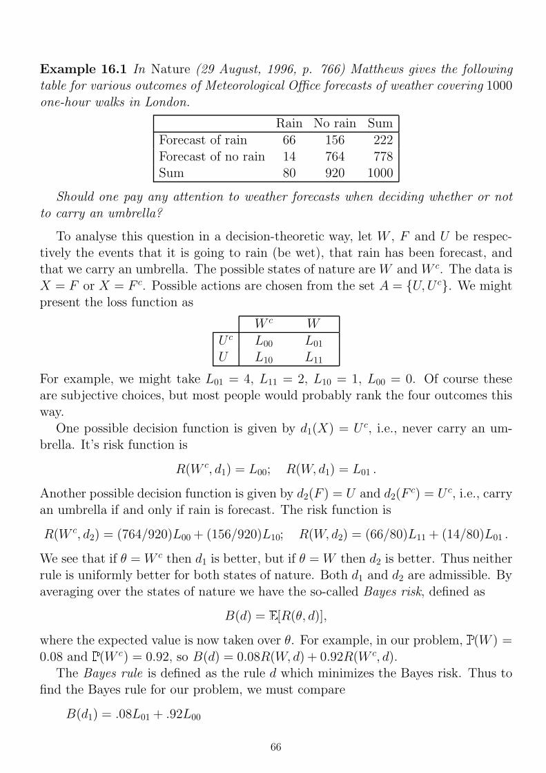
Example 6.1 It has been suggested that dying people may be able to postponetheir death until after an important occasion. In a study of 1919 people with Jewishsurnames it was found that 922 occurred in the week before Passover and 997 in theweek after. Is there any evidence in this data to reject the hypothesis that a personis as likely to die in the week before as in the week after Passover?
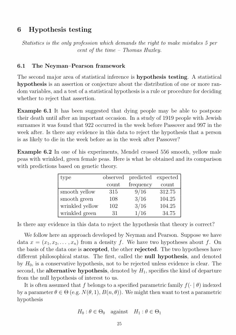
Example 6.2 In one of his experiments, Mendel crossed 556 smooth, yellow malepeas with wrinkled, green female peas. Here is what he obtained and its comparisonwith predictions based on genetic theory.
type observed predicted expectedcount frequency count
smooth yellow 315 9/16 312.75smooth green 108 3/16 104.25wrinkled yellow 102 3/16 104.25wrinkled green 31 1/16 34.75
Is there any evidence in this data to reject the hypothesis that theory is correct?
We follow here an approach developed by Neyman and Pearson. Suppose we havedata x = (x1, x2, . . . , xn) from a density f . We have two hypotheses about f . Onthe basis of the data one is accepted, the other rejected. The two hypotheses havedifferent philosophical status. The first, called the null hypothesis, and denotedby H0, is a conservative hypothesis, not to be rejected unless evidence is clear. Thesecond, the alternative hypothesis, denoted by H1, specifies the kind of departurefrom the null hypothesis of interest to us.
It is often assumed that f belongs to a specified parametric family f(· | θ) indexedby a parameter θ ∈ Θ (e.g.N(θ, 1),B(n, θ)). We might then want to test a parametrichypothesis
H0 : θ ∈ Θ0 against H1 : θ ∈ Θ1
25
with Θ0 ∩Θ1 = ∅. We may, or may not, have Θ0 ∪Θ1 = Θ.We will usually be concerned with testing a parametric hypothesis of this kind,
but alternatively, we may wish to test
H0 : f = f0 against H1 : f 6= f0
where f0 is a specified density. This is a ‘goodness-of-fit’ test.A third alternative is that we wish to test
H0 : f = f0 against H1 : f = f1
where f0 and f1 are specified, but do not necessarily belong to the same family.
6.2 Terminology
A hypothesis which specifies f completely is called simple, e.g., θ = θ0. Otherwise,a hypothesis is composite, e.g., θ > θ0.
Suppose we wish to test H0 against H1. A test is defined by a critical region C.We write C for the complement of C.
If x = (x1, x2, . . . , xn) ∈C then H0 is rejected, and
C then H0 is accepted (not rejected).
Note that when x ∈ C we might sometimes prefer to say ‘not rejected’, ratherthan ‘accepted’. This is a minor point which need not worry us, except to notethat sometimes ‘not rejected’ does more accurately express what we are doing: i.e.,looking to see if the data provides any evidence to reject the null hypothesis. If itdoes not, then we might want to consider other things before finally ‘accepting H0’.
There are two possible types of error we might make:
H0 might be rejected when it is true (a type I error), or
H0 might be accepted when it is false (a type II error).
Since H0 is conservative, a type I error is generally considered to be ‘more serious’that a type II error. For example, the jury in a murder trial should take as its nullhypothesis that the accused is innocent, since the type I error (that an innocentperson is convicted and the true murderer is never caught) is more serious than thetype II error (that a murderer is acquitted).
Hence, we fix (an upper bound on) the probability of type I error, e.g., 0.05 or0.01, and define the critical region C by minimizing the type II error subject to this.
If H0 is simple, Θ0 = θ0, the probability of a type I error is called the size,or significance level, of the test. If H0 is composite, the size of the test is α =supθ∈Θ0
P(X ∈ C | θ). .
26
The likelihood of a simple hypothesis H : θ = θ∗ given data x is
Lx(H) = fX(x | θ = θ∗).
If H is composite, H : θ ∈ Θ, we define
Lx(H) = supθ∈Θ
fX(x | θ).
The likelihood ratio for two hypotheses H0, H1 is
Lx(H0, H1) =Lx(H1)
Lx(H0).
Notice that if T (x) is a sufficient statistic for θ then by the factorization criterionLx(H0, H1) is simply a function of T (x).
6.3 Likelihood ratio tests
A test given by a critical region C of the form C = x : Lx(H0, H1) > k, for someconstant k, is called a likelihood ratio test. The value of k is determined by fixingthe size α of the test, so that P(X ∈ C | H0) = α.
Likelihood ratio tests are optimal for simple hypotheses. Most standard tests arelikelihood ratio tests, though tests can be built from others statistics.
Lemma 6.3 (Neyman–Pearson Lemma) H0 : f = f0 is to be tested against H1 :f = f1. Assume that f0 and f1 are > 0 on the same regions and continuous.
Then, among all tests of size ≤ α, the test with smallest probability of type II erroris given by C = x : f1(x)/f0(x) > k, where k is determined by
α = P(X ∈ C | H0) =
∫C
f0(x) dx.
Proof. Consider any test with size ≤ α, i.e., with a critical region D such thatP(X ∈ D | H0) ≤ α. Define
φD(x) =
10
as x∈6∈ D
and let C and k be defined as above. Note that
0 ≤(φC(x)− φD(x)
)(f1(x)− kf0(x)
), for all x.
since this is always the product of two terms with the same sign. Hence
0 ≤∫x
(φC(x)− φD(x)
)(f1(x)− kf0(x)
)dx
= P(X ∈ C | H1)− P(X ∈ D | H1)− k[P(X ∈ C | H0)− P(X ∈ D | H0)
]= P(X ∈ C | H1)− P(X ∈ D | H1)− k
[α− P(X ∈ D | H0)
]≤ P(X ∈ C | H1)− P(X ∈ D | H1)
This implies P(X 6∈ C | H1) ≤ P(X 6∈ D | H1) as required.
27
6.4 Single sample: testing a given mean, simple alternative, known vari-ance (z-test)
Let X1, . . . , Xn be IID N(µ, σ2), where σ2 is known. We wish to test H0 : µ = µ0
against H1 : µ = µ1, where µ1 > µ0.The Neyman–Pearson test is to rejectH0 if the likelihood ratio is large (i.e., greater
than some k). The likelihood ratio is
f(x | µ1, σ2)
f(x | µ0, σ2)=
(2πσ2)−n/2 exp[−∑n
i=1(xi − µ1)2/2σ2
](2πσ2)−n/2 exp [−
∑ni=1(xi − µ0)2/2σ2]
= exp
[n∑i=1
(xi − µ0)
2 − (xi − µ1)2 /2σ2
]= exp
[n
2x(µ1 − µ0) + (µ20 − µ2
1)/2σ2]
It often turns out, as here, that the likelihood ratio is a monotone function of asufficient statistic and we can immediately rephrase the critical region in more con-venient terms. We notice that the likelihood ratio above is increasing in the sufficientstatistic x (since µ1 − µ0 > 0). So the Neyman–Pearson test is equivalent to ‘rejectH0 if x > c’, where we choose c so that P(X > c | H0) = α. There is no need to tryto write c in terms of k.
However, under H0 the distribution of X is N(µ0, σ2/n). This means that
Z =√n(X − µ0)/σ ∼ N(0, 1) .
It is now convenient to rephrase the test in terms of Z, so that a test of size α is toreject H0 if z > zα, where zα = Φ−1(1− α) is the ‘upper α point of N(0, 1)’ i.e., thepoint such that P(N(0, 1) > zα) = α. E.g., for α = 0.05 we would take zα = 1.645,since 5% of the standard normal distribution lies to the right of 1.645.
Because we reject H0 only if z is in the upper tail of the normal distribution wecall this a one-tailed test. We shall see other tests in which H0 is rejected if thetest statistic lies in either of two tails. Such a test is called a two-tailed test.
Example 6.4 Suppose X1, . . . , Xn are IID N(µ, σ2) as above, and we want a testof size 0.05 of H0 : µ = 5 against H1 : µ = 6, with σ2 = 1. Suppose the data isx = (5.1, 5.5, 4.9, 5.3). Then x = 5.2 and z = 2(5.2 − 5)/1 = 0.4. Since this is lessthan 1.645 we do not reject µ = 5.
Suppose the hypotheses are reversed, so that we testH0 : µ = 6 againstH1 : µ = 5.The test statistic is now z = 2(5.2− 6)/1 = −1.6 and we should reject H0 for valuesof Z less than −1.645. Since z is more than −1.645, it is not significant and we donot reject µ = 6.
This example demonstrates the preferential position given to H0 and thereforethat it is important to choose H0 in a way that makes sense in the context of thedecision problem with which the statistical analysis is concerned.
28
7 Further aspects of hypothesis testing
Statisticians do it with only a 5% chance of being rejected.
7.1 The p-value of an observation
The significance level of a test is another name for α, the size of the test. For acomposite hypothesis H0 : θ ∈ Θ0 and rejection region C this is
α = supθ∈Θ0
P(X ∈ C | θ) .
For a likelihood ratio test the p-value of an observation x is defined to be
p∗ = supθ∈Θ0
Pθ(LX(H0, H1) ≥ Lx(H0, H1)
).
The p-value of x is the probability under H0 of seeing x or something at least as‘extreme’, in the sense of containing at least as much evidence against H0. E.g., inExample 6.4, the p-value is p∗ where
p∗ = P(Z > z | µ = µ0) = 1− Φ(z) .
A test of size α rejects H0 if and only if α ≥ p∗. Thus the p-value of x is thesmallest value of α for which H0 would be rejected on the basis of seeing x. It is oftenmore informative to report the p-value than merely to report whether or not the nullhypothesis has been rejected.
The p-value is also sometimes called the significance level of x. Historically, theterm arises from the practice of ‘significance testing’. Here, we begin with an H0
and a test statistic T , which need not be the likelihood ratio statistic, for which, say,large positive values suggest falsity of H0. We observe value t0 for the statistic: thesignificance level is P(T ≥ t0 | H0). If this probability is small, H0 is rejected.
7.2 The power of a test
For a parametric hypothesis about θ ∈ Θ, we define the power function of the testspecified by the critical region C as
W (θ) = P(X ∈ C | θ).
Notice that α = supθ∈Θ0W (θ), and 1−W (θ) = P(X ∈ C | θ) = P(type II error | θ)
for θ ∈ Θ1.
29
7.3 Uniformly most powerful tests
For the test of H0 : µ = µ0 against H1 : µ = µ1, µ1 > µ0 described in section 6.4 thecritical region turned out to be
C(µ0) =x :√n(x− µ0)/σ > αz
.
This depends on µ0 but not on the specific value of µ1. The test with this criticalregion would be optimal for any alternative H1 : µ = µ1, provided µ1 > µ0. This isthe idea of a uniformly most powerful (UMP) test.
We can find the power function of this test.
W (µ) = P(Z > αz | µ)
= P(√
n(X − µ0)/σ > αz | µ)
= P(√
n(X − µ)/σ +√n(µ− µ0
)/σ > αz | µ)
= 1− Φ(αz −
√n(µ− µ0)/σ
)Note that W (µ) increases from 0 to 1 as µ goes from −∞ to ∞ and W (µ0) = α.
More generally, suppose H0 : θ ∈ Θ0 is to be tested against H1 : θ ∈ Θ1, whereΘ0 ∩Θ1 = ∅. Suppose H1 is composite. H0 can be simple or composite. We want atest of size α. So we require W (θ) ≤ α for all θ ∈ Θ0, W (θ0) = α for some θ0 ∈ Θ0.
A uniformly most powerful (UMP) test of size α satisfies (i) it is of size α, (ii)W (θ) is as large as possible for every θ ∈ Θ1.
UMP tests may not exist. However, likelihood ratio tests are often UMP.
Example 7.1 Let X1, . . . , Xn be IID N(µ, σ2), where µ is known. Suppose H0 :σ2 ≤ 1 is to be tested against H1 : σ2 > 1.
We begin by finding the most powerful test for testing H ′0 : σ2 = σ20 against
H ′1 : σ2 = σ21, where σ2
0 ≤ 1 < σ21. The Neyman–Pearson test rejects H ′0 for large
values of the likelihood ratio:
f(x | µ, σ2
1)
f(x | µ, σ2
0
) =
(2πσ2
1)−n/2
exp[−∑n
i=1(xi − µ)2/2σ21](
2πσ20
)−n/2exp[−∑n
i=1(xi − µ)2/2σ20
]= (σ0/σ1)
n exp
[(1
2σ20− 1
2σ21
) n∑i=1
(xi − µ)2
]which is large when
∑i(xi − µ)2 is large. If σ2 = 1 then
n∑i=1
(xi − µ)2 ∼ χ2n .
So a test of the form ‘reject H0 if T :=∑
i(xi − µ)2 > F(n)α ’, has size α where F
(n)α
is the upper α point of χ2n. That is, P
(T > F
(n)α | σ2 ≤ 1
)≤ α, for all σ2 ≤ 1, with
30
equality for σ2 = 1. But this test doesn’t depend on the value of σ21, and hence is
the UMP test of H0 against H1.
Example 7.2 Consider Example 6.1. Let p be the probability that if a death occursin one of the two weeks either side of Passover it actually occurs in the week afterthe Passover. Let us test H0 : p = 0.5 vs. H1 : p > 0.5.
The distribution of the number of deaths in the week after Passover, say X,is B(n, p), which we can approximate by N
(np, np(1 − p)
); under H0 this is
N(0.5n, 0.25n). So a size 0.05 test is to reject H0 if z =√n(x − µ0
)/σ > 1.645,
where here z =√
1919(997/1919− 0.5
)/0.5 = 1.712. So the data is just significant
at the 5% level. We reject the hypothesis that death p = 1/2.It is important to realise that this does not say anything about why this might
be. It might be because people really are able to postpone their deaths to enjoythe holiday. But it might also be that deaths increase after Passover because ofover-eating or stress during the holiday.
7.4 Confidence intervals and hypothesis tests
There is an interesting duality between confidence intervals and hypothesis tests.In the following, we speak of the acceptance region, i.e., the complement of thecritical (or rejection) region C.
Theorem 7.3
(i) Suppose that for every θ0 there is a size α test of H0 : θ = θ0 against somealternative. Denote the acceptance region by A(θ0). Then I(X) = θ : X ∈A(θ) is a 100(1− α)% confidence interval for θ.
(ii) Conversely, if I(X) is a 100(1−α)% confidence interval for θ then an acceptanceregion for a size α test of H0 : θ = θ0 is A(θ0) = X : θ0 ∈ I(X).
Proof. The definitions in the theorem statement give
P(X ∈ A(θ0) | θ = θ0
)= P
(θ ∈ I(X) | θ = θ0
).
By assumption the l.h.s. is 1− α in case (i) and the r.h.s. is 1− α in case (ii).
This duality can be useful. In some circumstances it can be easier to see whatis the form of a hypothesis test and then work out a confidence interval. In othercircumstances it may be easier to see the form of the confidence interval.
In Example 4.1 we saw that a 95% confidence interval for µ based upon X1, . . . , Xn
being IID samples from N(µ, σ2), σ2 known, is[X − 1.96σ√
n, X +
1.96σ√n
].
31
Thus H0 : µ = µ0 is rejected in a 5% level test against H1 : µ 6= µ0 if and only if µ0
is not in this interval; i.e., if and only if√n∣∣X − µ0
∣∣/σ > 1.96 .
7.5 The Bayesian perspective on hypothesis testing
Suppose a statistician wishes to test the hypothesis that a coin is fair (H0 : p = 1/2)against the alternative that it biased towards heads with probability p, (H1 : p =p1 > 1/2). He decides to toss it five times. It is easy to see that the best test is toreject H0 if the total number of heads, say T , is large. Here T ∼ B(5, p). Supposehe observes H,H,H,H,T, so T = 4. The p-value (or significance level) of this result isthe probability that under the null hypothesis he should see a result which is equallyor more extreme, i.e.,
Another statistician wishes also wishes to test H0 against H1, but with a differentexperiment. He plans to toss the coin until he gets a tail. Now the best test isto reject H0 if the number of tosses, say N , is large. Here N ∼ geometric(1 − p).Suppose this statistician also observes H,H,H,H,T, so N = 5. He figures the p-valueas the probability of seeing this result or one that is even more extreme and obtains
P(N ≥ 5) = 0.54 = 1/16 = 0.0625 .
Thus the two statisticians come to different conclusions about the significanceof what they have seen. This is disturbing! The coin knew nothing about theexperimental procedure. Maybe there were four tosses simply because that was thepoint at which the experimenter spilt his coffee and so decided to stop tossing thecoin. What then is the significance level?
The Bayesian perspective on hypothesis testing avoids this type of problem. Sup-pose the experimenter places prior probabilities of P(H0) and P(H1) on the truth oftwo mutually exclusive hypotheses. Having observed the data x, these are modifiedinto posterior probabilities in the usual way, i.e.,
P(H1 | x)
P(H0 | x)=P(x | H1)
P(x | H0)
P(H1)
P(H0)= Lx(H0, H1)
P(H1)
P(H0).
Thus the ratio of the posterior probabilities is just the ratio of the prior probabilitiesmultiplied by the likelihood ratio.
Under both procedures above x = H,H,H,H,T, and the likelihood ratios is
Lx(H0, H1) =p1
0.5× p1
0.5× p1
0.5× p1
0.5× (1− p1)
0.5=p4
1(1− p1)
0.55 .
In general, the Bayesian analysis does not depend on how the data was obtained.
32
8 Generalized likelihood ratio tests
An approximate answer to the right problem is worth a good deal more than anexact answer to an approximate problem.
8.1 The χ2 distribution
This distribution plays a huge role in Statistics. For n a positive integer, the χ2n
distribution is the distribution of
X21 + · · ·+X2
n, where X1, . . . , Xn are IID each N(0, 1).
It is not difficult to show that
χ2n = gamma
(12n,
12
),
with pdf
f(t) = (12)n/2tn/2−1e−t/2
/Γ(n/2), t > 0 .
We speak of the ‘chi-squared distribution with (or on) n degrees of freedom’. IfX ∼ χ2
n, E (X) = n, var(X) = 2n.
8.2 Generalised likelihood ratio tests
Tests with critical regions of the form C = x : Lx(H0, H1) > k are intuitivelysensible, and in certain cases optimal. But such a critical region may not reduceto a region depending only on the value of a simple function T (x). Even if it does,the distribution of the statistic T (X), required to determine k, may not be simple.However, the following theorem allows us to use a likelihood ratio test even in thiscase. We must take care in describing the circumstances for which the theorem isvalid.
So far we have considered disjoint alternatives, but if our real interest is in testingH0 and we are not interested in any specific alternative it is simpler to take (in theparametric framework) Θ1 = Θ, rather than Θ1 = Θ \Θ0.
So we now suppose we are testing H0 : θ ∈ Θ0 against H1 : θ ∈ Θ, i.e., a nullhypothesis which restricts θ against a general alternative.
Suppose that with this formulation Θ0 imposes p independent restrictions on θ,so that, for example, we have Θ = θ : θ = (θ1, . . . , θk) and
H0 : θi1 = α1, . . . , θip = αp, for given αj ; or
H0 : Aθ = b, for given Ap×k, bp×1 ; or
H0 : θi = θi(φ1, . . . , φk−p), i = 1, . . . , k, for given θ1(·), . . . , θk(·)and φ1, . . . , φk−p to be estimated.
33
Θ1 has k free parameters and Θ0 has k − p free parameters. We write |Θ1| = k and|Θ0| = k − p. Then we have the following theorem (not to be proved.)
Theorem 8.1 Suppose Θ0 ⊂ Θ1 and |Θ1|−|Θ0| = p. Then under certain conditions,as n→∞ with X = (X1, . . . , Xn) and Xi IID,
2 logLX(H0, H1) ∼ χ2p,
if H0 is true. If H0 is not true, 2 logLX tends to be larger. We reject H0 if 2 logLx >c, where α = P
(χ2p > c
)to give a test of size approximately α.
We say that 2 logLX(H0, H1) is asymptotically distributed as χ2p. The conditions
required by the theorem hold in all the circumstances we shall meet in this course.
Lemma 8.2 Suppose X1, . . . , Xn are IID N(µ, σ2). Then
(i) maxµ f(x | µ, σ2) = (2πσ2)−n/2 exp[−∑
i(xi − x)2/2σ2].
(ii) maxσ2 f(x | µ, σ2) =[2π
∑i(xi−µ)2
n
]−n/2exp [−n/2].
(iii) maxµ,σ2 f(x | µ, σ2) =[2π
∑i(xi−x)2
n
]−n/2exp [−n/2].
8.3 Single sample: testing a given mean, known variance (z-test)
Let X1, . . . , Xn be IID N(µ, σ2), where σ2 is known. We wish to test H0 : µ = µ0
against H1 : µ 6= µ0. The generalized likelihood ratio test suggests that we shouldreject H0 if Lx(H0, H1) is large, where
Lx(H0, H1) =supµ f
(x | µ, σ2
)f(x | µ0, σ2
)=
(2πσ2
)−n/2exp
[−∑
i(xi − x)2/2σ2](
2πσ2)−n/2
exp[−∑
i(xi − µ0)2/2σ2]
= exp
[(1/2σ2)
n∑i=1
(xi − µ0)
2 − (xi − x)2]= exp
[(1/2σ2)n(x− µ0)
2]That is, we should reject H0 if (x− µ0)
2 is large.This is no surprise. For under H0, X ∼ N(µ0, σ
2/n), so that
Z =√n(X − µ0)/σ ∼ N(0, 1),
and a test of size α is to reject H0 if z > zα/2 or if z < −zα/2, where zα/2 is the ‘upperα/2 point of N(0, 1)’ i.e., the point such that P(N(0, 1) > zα/2) = α/2. This is anexample of a two-tailed test.
34
Note that 2 logLX(H0, H1) = Z2 ∼ χ21. In this example H0 imposes p = 1
constraint on the parameter space and the approximation in Theorem 8.1 is exact.
8.4 Single sample: testing a given variance, known mean (χ2-test)
As above, let X1, . . . , Xn be IID N(µ, σ2), where µ is known. We wish to testH0 : σ2 = σ2
0 against H1 : σ2 6= σ20. The generalized likelihood ratio test suggests
that we should reject H0 if Lx(H0, H1) is large, where
Lx(H0, H1) =supσ2 f
(x | µ, σ2
)f(x | µ, σ2
0
) =
[2π∑i(xi−µ)2
n
]−n/2exp [−n/2]
(2πσ20)−n/2 exp
[−∑
i(xi − µ)2/2σ20
] .If we let t =
∑i(xi − µ)2/nσ2
0 we find
2 logLx(H0, H1) = n(t− 1− log t) ,
which increases as t increases from 1 and t decreases from 1. Thus we should rejectH0 when the difference of t and 1 is large.
Again, this is not surprising, for under H0,
T =n∑i=1
(Xi − µ)2/σ20 ∼ χ2
n .
So a test of size α is the two-tailed test which rejects H0 if t > F(n)α/2 or t < F
(n)1−α/2
where F(n)1−α/2 and F
(n)α/2 are the lower and upper α/2 points of χ2
n, i.e., the points such
that P(χ2n < F
(n)1−α/2
)= P
(χ2n > F
(n)α/2
)= α/2.
8.5 Two samples: testing equality of means, known common variance(z-test)
Let X1, . . . , Xm be IID N(µ1, σ2) and let Y1, . . . , Yn be IID N(µ2, σ
2), and supposethat the two samples are independent. It is required to test H0 : µ1 = µ2 againstH1 : µ1 6= µ2. The likelihood ratio test is based on
Lx(H0, H1) =supµ1,µ2
f(x | µ1, σ
2)f(y | µ2, σ
2)
supµ f(x | µ, σ2
)f(y | µ, σ2
)=
(2πσ2)−(m+n)/2 exp[−∑
i(xi − x)2/2σ2]
exp[−∑
i(yi − y)2/2σ2]
(2πσ2)−(m+n)/2 exp[−∑
i
(xi − mx+ny
m+n
)2/2σ2
]exp
[−∑
i
(yi − mx+ny
m+n
)2/2σ2
]= exp
[m
2σ2
(x− mx+ ny
m+ n
)2
+n
2σ2
(y − mx+ ny
m+ n
)2]
= exp
[1
2σ2
mn
(m+ n)(x− y)2
]35
So we should reject H0 if |x − y| is large. Now, X ∼ N(µ1, σ2/m) and Y ∼
N(µ2, σ2/n), and the samples are independent, so that, on H0,
X − Y ∼ N
(0, σ2
(1
m+
1
n
))or
Z = (X − Y )
(1
m+
1
n
)− 12 1
σ∼ N(0, 1).
A size α test is the two-tailed test which rejects H0 if z > zα/2 or if z < −zα/2, wherezα/2 is, as in 8.3 the upper α/2 point of N(0, 1). Note that 2 logLX(H0, H1) = Z2 ∼χ2
1, so that for this case the approximation in Theorem 8.1 is again exact.
8.6 Goodness-of-fit tests
Suppose we observe n independent trials and note the numbers of times that eachof k possible outcomes occurs, i.e., (x1, . . . , xk), with
∑j xj = n. Let pi be the
probability of outcome i. On the basis of this data we want to test the hypothesisthat p1, . . . , pk take particular values. We allow that these values might depend onsome unknown parameter θ (or parameters if θ is a vector). I.e., we want to test
H0 : pi = pi(θ) for θ ∈ Θ0 against H1 : pi are unrestricted.
For example, H0 might be the hypothesis that the trials are samples from a binomialdistribution B(k, θ), so that under H0 we would have pi(θ) =
(ki
)θi(1− θ)k−i.
This is called a goodness-of-fit test, because we are testing whether our datafit a particular distribution (in the above example the binomial distribution).
The distribution of (x1, . . . , xk) is the multinomial distribution
P(x1, . . . , xk | p) =n!
x1! · · ·xk!px1
1 · · · pxkk ,
for (x1, . . . , xk) s.t. xi ∈ 0, . . . , n and∑k
i=1 xi = n. Then we have
supH1
log f(x) = const + sup
k∑i=1
xi log pi
∣∣∣∣∣ 0 ≤ pi ≤ 1,k∑i=1
pi = 1
.
Now,∑
i xi log pi may be maximised subject to∑
i pi = 1 by a Lagrangian techniqueand we get pi = xi/n. Likewise,
supH0
log f(x) = const + supθ
k∑i=1
xi log pi(θ)
.
The generalized likelihood tells us to reject H0 if 2Lx(H0, H1) is large compared tothe chi-squared distribution with d.f. |Θ1| − |Θ0|. Here |Θ1| = k − 1 and |Θ0| is thenumber of independent parameters to be estimated under H0.
36
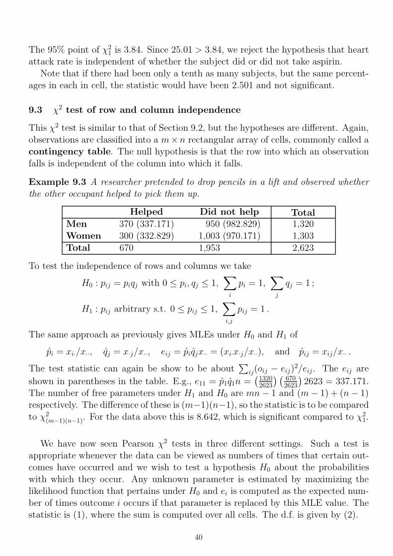
9 Chi-squared tests of categorical data
A statistician is someone who refuses to play the national lottery,but who does eat British beef. (anonymous)
9.1 Pearson’s chi-squared statistic
Suppose, as in Section 8.6, that we observe x1, . . . , xk, the numbers of times thateach of k possible outcomes occurs in n independent trials, and seek to make thegoodness-of-fit test of
H0 : pi = pi(θ) for θ ∈ Θ0 against H1 : pi are unrestricted.
Recall
2 logLx(H0, H1) = 2k∑i=1
xi log pi − 2k∑i=1
xi log pi(θ) = 2k∑i=1
xi log(pi/pi(θ)
),
where pi = xi/n and θ is the MLE of θ under H0. Let oi = xi denote the numberof time that outcome i occurred and let ei = npi(θ) denote the expected number oftimes it would occur under H0. It is usual to display the data in k cells, writing oiin cell i. Let δi = oi − ei. Then
2 logLx(H0, H1) = 2k∑i=1
xi log((xi/n)/pi(θ)
)= 2
k∑i=1
oi log(oi/ei)
= 2k∑i=1
(δi + ei) log(1 + δi/ei)
= 2k∑i=1
(δi + ei)(δi/ei − δ2i /2e
2i + · · ·)
+
k∑i=1
δ2i /ei
=k∑i=1
(oi − ei)2
ei(1)
This is called the Pearson chi-squared statistic.For H0 we have to choose θ. Suppose the optimization over θ has p degrees of
freedom. For H1 we have k − 1 parameters to choose. So the difference of these
37
degrees of freedom is k − p − 1. Thus, if H0 is true the statistic (1) ∼ χ2k−p−1
approximately. A mnemonic for the d.f. is
d.f. = #(cells) − #(parameters estimated) −1. (2)
Note that
k∑i=1
(oi − ei)2
ei=
k∑i=1
[o2i
ei− 2oi + ei
]=
k∑i=1
o2i
ei− 2n+ n =
k∑i=1
o2i
ei− n . (3)
Sometimes (3) is easier to compute than (1).
Example 9.1 For the data from Mendel’s experiment, the test statistic has the value0.618. This is to be compared to χ2
3, for which the 10% and 95% points are 0.584and 7.81. Thus we certainly do not reject the theoretical model. Indeed, we wouldexpect the observed counts to show even greater disparity from the theoretical modelabout 90% of the time.
Similar analysis has been made of many of Mendel’s other experiments. The dataand theory turn out to be too close for comfort. Current thinking is that Mendel’stheory is right but that his data were massaged by somebody (Fisher thought it wasMendel’s gardening assistant) to improve its agreement with the theory.
9.2 χ2 test of homogeneity
Suppose we have a rectangular array of cells with m rows and n columns, with Xij
items in the (i, j) th cell of the array. Denote the row, column and overall sums by
Xi· =n∑j=1
Xij, X·j =m∑i=1
Xij, X·· =m∑i=1
n∑j=1
Xij.
Suppose the row sums are fixed and the distribution of (Xi1, . . . , Xin) in row i ismultinomial with probabilities (pi1, . . . , pin), independently of the other rows. Wewant to test the hypothesis that the distribution in each row is the same, i.e., H0 : pijis the same for all i, (= pj) say, for each j = 1, . . . , n. The alternative hypothesis isH1 : pij are unrestricted. We have
log f(x) = const +∑i
∑j
xij log pij , so that
supH1
log f(x) = const + sup
m∑i=1
n∑j=1
xij log pij
∣∣∣∣∣ 0 ≤ pij ≤ 1,n∑j=1
pij = 1 ∀i
Now,∑
j xij log pij may be maximized subject to∑
j pij = 1 by a Lagrangian tech-
nique. The maximum of∑
j xij log pij + λ(
1−∑
j pij
)occurs when xij/pij = λ,
38
∀j. Then the constraints give λ =∑
j xij and the corresponding maximizing pij ispij = xij/
∑j xij = xij/xi·. Hence,
supH1
log f(x) = const +m∑i=1
n∑j=1
xij log(xij/xi·).
Likewise,
supH0
logf(x) = const + sup
∑i
∑j
xij log pj
∣∣∣∣∣ 0 ≤ pj ≤ 1,∑j
pj = 1
,
= const +∑i
∑j
xij log(x·j/x··).
Here pj = x·j/x··. Let oij = xij and write eij = pjxi· = (x·j/x··)xi· for the expectednumber of items in position (i, j) under H0. As before, let δij = oij − eij. Then,
2 logLx(H0, H1) = 2∑i
∑j
xij log(xijx··/xi·x·j)
= 2∑i
∑j
oij log(oij/eij)
= 2∑i
∑j
(δij + eij) log(1 + δij/eij)
+
∑i
∑j
δ2ij/eij
=∑i
∑j
(oij − eij)2/eij . (4)
For H0, we have (n−1) parameters to choose, for H1 we have m(n−1) parametersto choose, so the degrees of freedom is (n − 1)(m − 1). Thus, if H0 is true thestatistic (4) ∼ χ2
(n−1)(m−1) approximately.
Example 9.2 The observed (and expected) counts for the study about aspirin andheart attacks described in Example 1.2 are
The 95% point of χ21 is 3.84. Since 25.01 > 3.84, we reject the hypothesis that heart
attack rate is independent of whether the subject did or did not take aspirin.Note that if there had been only a tenth as many subjects, but the same percent-
ages in each in cell, the statistic would have been 2.501 and not significant.
9.3 χ2 test of row and column independence
This χ2 test is similar to that of Section 9.2, but the hypotheses are different. Again,observations are classified into a m×n rectangular array of cells, commonly called acontingency table. The null hypothesis is that the row into which an observationfalls is independent of the column into which it falls.
Example 9.3 A researcher pretended to drop pencils in a lift and observed whetherthe other occupant helped to pick them up.
Helped Did not help TotalMen 370 (337.171) 950 (982.829) 1,320Women 300 (332.829) 1,003 (970.171) 1,303
Total 670 1,953 2,623
To test the independence of rows and columns we take
H0 : pij = piqj with 0 ≤ pi, qj ≤ 1,∑i
pi = 1,∑j
qj = 1 ;
H1 : pij arbitrary s.t. 0 ≤ pij ≤ 1,∑i,j
pij = 1 .
The same approach as previously gives MLEs under H0 and H1 of
pi = xi·/x··, qj = x·j/x··, eij = piqjx·· = (xi·x·j/x··), and pij = xij/x·· .
The test statistic can again be show to be about∑
ij(oij − eij)2/eij. The eij are
shown in parentheses in the table. E.g., e11 = p1q1n =(1320
2623
) ( 6702623
)2623 = 337.171.
The number of free parameters under H1 and H0 are mn− 1 and (m− 1) + (n− 1)respectively. The difference of these is (m−1)(n−1), so the statistic is to be comparedto χ2
(m−1)(n−1). For the data above this is 8.642, which is significant compared to χ21.
We have now seen Pearson χ2 tests in three different settings. Such a test isappropriate whenever the data can be viewed as numbers of times that certain out-comes have occurred and we wish to test a hypothesis H0 about the probabilitieswith which they occur. Any unknown parameter is estimated by maximizing thelikelihood function that pertains under H0 and ei is computed as the expected num-ber of times outcome i occurs if that parameter is replaced by this MLE value. Thestatistic is (1), where the sum is computed over all cells. The d.f. is given by (2).
40
10 Distributions of the sample mean and variance
Statisticians do it. After all, it’s only normal.
10.1 Simpson’s paradox
Example 10.1 These are some Cambridge admissions statistics for 1996.
In all five subjects women have an equal or better success rate in applications thando men. However, taken overall, 24% of men are successful but only 23% of womenare successful! This is called Simpson’s paradox (though it was actually discoveredby Yule 50 years earlier). It can often be found in real data. Of course it is not aparadox. The explanation here is that women are more successful in each subject,but tend to apply more for subjects that are hardest to get into (e.g., Veterinarymedicine). This example should be taken as a warning that pooling contingencytables can produce spurious associations. The correct interpretation of this data isthat, for these five subjects, women are significantly more successful in gaining entrythan are men.
In order to produce an example of Simpson’s paradox I carefully selected fivesubjects from tables of 1996 admissions statistics. Such ‘data snooping’ is cheating; asimilar table that reversed the roles of men and women could probably be constructedby picking different subjects.
10.2 Transformation of variables
The rest of this lecture is aimed at proving some important facts about distributionof the statistics X and SXX =
∑i(Xi− X)2, when X1, . . . , Xn are IID N(µ, σ2). We
begin by reviewing some ideas about transforming random variables.
Suppose the joint density of X1, . . . , Xn is fX , and there is a 1–1 mapping betweenX1, . . . , Xn and Y1, . . . , Yn such that Xi = xi(Y1, . . . , Yn). Then the joint density of
41
Y1, . . . , Yn is
fY (y1, . . . , yn) = fX(x1(y), . . . , xn(y))
∣∣∣∣∣∣∣∂x1(y)∂y1
· · · ∂x1(y)∂yn
......
∂xn(y)∂y1
· · · ∂xn(y)∂yn
∣∣∣∣∣∣∣where the Jacobian := J(y1, . . . , yn) is the absolute value of the determinant of thematrix (∂xi(y)/∂yj).
The following example is an important one, which also tells us more about thebeta distribution.
Example 10.2 Let X1 ∼ gamma(n1, λ) and X2 ∼ gamma(n2, λ), independently.Let Y1 = X1/(X1 + X2), Y2 = X1 + X2. Since X1 and X2 are independent wemultiply their pdfs to get
fX(x) =λn1xn1−1
1
(n1 − 1)!e−λx1 × λn2xn2−1
2
(n2 − 1)!e−λx2.
Then x1 = y1y2, x2 = y2 − y1y2, so
J(y1, y2) =
∣∣∣∣∣∂x1(y)∂y1
∂x1(y)∂y2
∂x2(y)∂y1
∂x2(y)∂y2
∣∣∣∣∣ =
∣∣∣∣ y2 y1
−y2 1− y1
∣∣∣∣ = y2
Hence making the appropriate substitutions and arranging terms we get
fY (y) =(n1 + n2 − 1)!
(n1 − 1)!(n2 − 1)!yn1−1
1 (1− y1)n2−1 × λn1+n2yn1+n2−1
2
(n1 + n2 − 1)!e−λy2
from which it follows that Y1 and Y2 are independent RVs (since their joint den-sity function factors into marginal density functions) and Y1 ∼ beta(n1, n2), Y2 ∼gamma(n1 + n2, λ).
10.3 Orthogonal transformations of normal variates
Lemma 10.3 Let X1, . . . , Xn, be independently distributed with distributionsN(µi, σ
2) respectively. Let A = (aij) be an orthogonal matrix, so that A>A =AA> = I. Then the elements of Y = AX are independently distributed, andYi ∼ N
((Aµ)i, σ
2), where µ = (µ1, . . . , µn)
>.
Proof. The joint density of X1, . . . , Xn is
fX(x1, . . . , xn | µ, σ2) =∏i
fXi(xi | µi, σ2)
=1
(2πσ2)n/2e−
∑i(xi−µi)2/2σ2
=1
(2πσ2)n/2e−(x−µ)>(x−µ)/2σ2
42
Since x = A>y, we have ∂xi/∂yj = aji and hence J(y1, . . . , yn) = | det(A>)| = 1.Thus
fY (y1, . . . , yn | µ, σ2) =1
(2πσ2)n/2exp
[−(A>y− µ)>(A>y − µ)/2σ2]
=1
(2πσ2)n/2exp
[−(A>y− A>Aµ)>(A>y −A>Aµ)/2σ2]
=1
(2πσ2)n/2exp
[−(y−Aµ)>AA>(y−Aµ)/2σ2]
=1
(2πσ2)n/2exp
[−(y−Aµ)>(y− Aµ)/2σ2]
Remark. An alternative proof can be given using moment generating functions.For θ ∈ Rn , the mgf of the joint distribution is
E exp[θ>Y
]= E exp
[θ>AX
]= E exp
[(A>θ)>X
]= exp
[(A>θ)>µ+ 1
2σ2(A>θ)>(A>θ)
]= exp
[θ>Aµ+ 1
2σ2θ>θ
]which we recognise as the mgf of independent RVs with distributions N
((Aµ)i, σ
2).
10.4 The distributions of X and SXX
Lemma 10.4 Let X1, . . . , Xn be IID N(µ, σ2) and let X = n−1∑ni=1Xi, SXX =∑n
i=1(Xi − X)2. Then:
(i) X ∼ N(µ, σ2/n) and n(X − µ)2 ∼ σ2χ21.
(ii) Xi − µ ∼ N(0, σ2), so∑n
i=1(Xi − µ)2 ∼ σ2χ2n.
(iii)∑n
i=1(Xi − µ)2 = SXX + n(X − µ)2.
(iv) SXX/(n− 1) is an unbiased estimator of σ2.
(v) X and SXX are independent.
(vi) SXX ∼ σ2χ2n−1.
Proof.
(i) and (ii) are immediate from the fact that linear combinations of normal RVsare normally distributed and the definition of χ2
n. To prove (iii) and (iv) we note
43
thatn∑i=1
(Xi − µ)2 =n∑i=1
([Xi − X] + [X − µ]
)2
=n∑i=1
([Xi − X]2 + 2[Xi − X][X − µ] + [X − µ]2
)= SXX + n[X − µ]2
Let A be an orthogonal matrix such that
Y = A(X− µ1) =
(√n(X − µ), Y2, . . . , Yn
).
I.e., we take
A =
1/√n 1/
√n · · · 1/
√n
......
...· · · · · ·
where the rows below the first are chosen to make the matrix orthogonal. ThenY1 =
√n(X − µ) ∼ N(0, σ2) and Y1 is independent of Y2, . . . , Yn. Since
∑ni=1 Y
2i =∑
i(Xi − µ)2, we must have
n∑i=2
Y 2i =
n∑i=1
(Xi − µ)2 − n(X − µ)2 = SXX .
Hence SXX and Y1 (and equivalently SXX and X) are independent. This gives (v).Finally, (vi) follows from SXX =
∑ni=2 Y
2i and the fact that Y2, . . . , Yn are IID
N(0, σ2).
10.5 Student’s t-distribution
If X ∼ N(0, 1), Y ∼ χ2n, independently of X, then
Z = X/(Y/n)12 ∼ tn,
where tn is the Student’s t-distribution with (or on) n degrees of freedom. Like thenormal distribution, this distribution is symmetric about 0, and bell-shaped, but hasmore probability in its tails, i.e., for all t > 0, P(Z > t) > P(X > t).
From Lemma 10.4 we have√n(X − µ) ∼ σN(0, 1) and SXX ∼ σ2χ2
n−1, indepen-dently. So from these and the definition of the t-distribution follows the importantfact that if X1, . . . , Xn are IID N(µ, σ2), then
√n(X − µ)√SXX/(n− 1)
∼ tn−1 .
44
11 The t-test
Statisticians do it with two-tail T tests.
11.1 Confidence interval for the mean, unknown variance
Suppose X1, . . . , Xn IID N(µ, σ2), but now σ2 is unknown. Recall
T =
√n(X − µ)
σ∼ tn−1 .
where σ2 = SXX/(n− 1). A 100(1− α)% confidence interval for µ follows from
1− α = P
(−t(n−1)
α/2 ≤√n(X − µ)
σ≤ t
(n−1)α/2
)= P
(X −
tα/2σ√n≤ µ ≤ X +
tα/2σ√n
)where t
(n−1)α/2 is the ‘upper α/2 point of a t-distribution on n− 1 degrees of freedom’,
i.e., such that P(T > t
(n−1)α/2
)= α/2.
Example 11.1 In ‘Sexual activity and the lifespan of male fruitflies’, Nature, 1981,Partridge and Farquhar report experiments which examined the cost of increased re-production in terms of reduced longevity for male fruitflies. They kept numbers ofmale flies under different conditions. 25 males in one group were each kept with 1receptive virgin female. 25 males in another group were each kept with 1 female whohad recently mated. Such females will refuse to remate for several days. These servedas a control for any effect of competition with the male for food or space. The groupswere treated identically in number of anaesthetizations (using CO2) and provision offresh food.
To verify ‘compliance’ two days per week throughout the life of each experimentalmale, the females that had been supplied as virgins to that male were kept and exam-ined for fertile eggs. The insemination rate declined from approximately 1 per day atage one week to about 0.6 per day at age eight weeks.
Here s.e. is an abbreviation for standard error, i.e. the value of σ =√Sxx/(n− 1). Here n = 25. The mean life, x and the s.e., σ, are sufficient statistics
for (µ, σ2), so there is nothing else we need to know about the individual values of
45
the the longevities of these 50 flies in order to compute confidence intervals or teststatistics.
From these summary statistics we can compute 95% confidence intervals for themean lives of the control and test groups to be
[64.80− 2.06(15.6526)/√
25, 64.80 + 2.06(15.6526)/√
25] = [58.35, 71.25]
[56.76− 2.06(14.9284)/√
25, 56.76 + 2.06(14.9284)/√
25] = [50.61, 62.91]
It is interesting to look at the data, and doing so helps us check that lifespan isnormally distributed about a mean. The longevities for control and test groups were
11.2 Single sample: testing a given mean, unknown variance (t-test)
Suppose that with the same assumptions as above it is required to test H0 : µ = µ0
against H1 : µ 6= µ0.Adopting the paradigm of the generalized likelihood ratio test we consider
Lx(H0, H1) =maxµ,σ2 f
(x | µ, σ2
)maxσ2 f
(x | µ0, σ2
)=
[2π∑
i(xi − x)2/n]−n/2
exp [−n/2]
[2π∑
i(xi − µ0)2/n]−n/2 exp [−n/2]
=
[∑i(xi − µ0)2∑i(xi − x)2
]n/2=
[∑i(xi − x)2 + n(x− µ0)
2∑i(xi − x)2
]n/2=
[1 +
n(x− µ0)2∑i(xi − x)2
]n/2.
This is large when T 2 := n(n− 1)(x−µ0)2/ ∑
i(xi− x)2 is large, equivalently when|T | is large. Under H0 we have T ∼ tn−1. So a size α test is the two-tailed test which
rejects H0 if t > t(n−1)α/2 or if t < −t(n−1)
α/2 .
Example 11.2 Does jogging lead to a reduction in pulse rate? Eight non-joggingvolunteers engaged in a one-month jogging programme. Their pulses were taken beforeand after the programme.
Although there are two sets of data it is really just the changes that matter. Let thedecreases in pulse rates be x1, . . . , x8 and assume these are samples from N(µ, σ2)for some unknown σ2. To test H0 : µ = 0 against H1 : µ 6= 0 we compute∑
xi = 22, x = 2.75,∑
x2i = 326, Sxx =
∑x2i − 8x2 = 265.5.
Hence the test statistic is
t =
√8(2.75− 0)√
265.5/(8− 1)= 1.263,
which is to be compared to t(7)0.025 = 2.365. Hence the data is not sufficient to reject
H0 at the 5% level. This may surprise you since 6 of the 8 subjects had lowered pulserates. This sort of test is called a paired samples t-test.
11.3 Two samples: testing equality of means, unknown common variance(t-test)
We have the same samples as in 8.5, i.e., X1, . . . , Xm are IID N(µ1, σ2) and Y1, . . . , Yn
are IID N(µ2, σ2). These two samples are independent. It is required to test H0 :
µ1 = µ2 against H1 : µ1 6= µ2, but now σ2 is unknown. Note how this differs fromthe paired t-test above: the samples are not paired, and can be of unequal sizes.
As above, a maximum likelihood approach could convince us that the test shouldbe of the form ‘reject H0 if (x− y)2/(Sxx + Syy) is large.
As in 8.5 we have that under H0,
(X − Y )
(1
m+
1
n
)− 12 1
σ∼ N(0, 1) .
If SXX =∑m
i=1(Xi − X)2, and SY Y =∑n
j=1(Yj − Y )2, then
(SXX + SY Y )/σ2 ∼ χ2m+n−2
so that (since X is independent of SXX , Y is independent of SY Y and the two samplesare independent)
T = (X − Y )
/√(1
m+
1
n
)(SXX + SY Ym+ n− 2
)∼ tm+n−2.
A test of size α rejects H0 if t > t(m+n−2)α/2 or if t < −t(m+n−2)
α/2 .
47
Example 11.3 For the fruitfly data we might test H0 : that mean longevity is thesame for males living with 8 interested females as with 8 uninterested females. Thetest statistic is
t = (64.80− 56.76)
/√(1
25+
1
25
)(24(15.6525) + 24(14.9284)
25 + 25− 2
)= 1.859
which can be compared to t(48)0.025 = 2.01, and therefore is not significant at the 0.05%
level. H0 is not rejected. (It is however, significant at the 10% level, since t(48)0.05 =
1.68).
Similarly, we can give a 95% confidence interval for the difference of the means.This has endpoints
(64.80− 56.76)± 2.01
√(1
25+
1
25
)(24(15.6525) + 24(14.9284)
25 + 25− 2
)= 8.04± 8.695.
I.e., a 95% confidence interval for the extra longevity of celibate males is[−0.655, 16.735] days. Notice again that finding we cannot reject µ1 − µ2 = 0 atthe 5% level is equivalent to finding that the 95% confidence interval for the differ-ence of the means contains 0.
In making the above test we have assumed that the variances for the two popula-tions are the same. In the next lecture we will see how we might test that hypothesis.
11.4 Single sample: testing a given variance, unknown mean (χ2-test)
Let X1, . . . , Xn be IID N(µ, σ2), and suppose we wish to test H0 : σ2 = σ20 against
H1 : σ2 6= σ20, where µ is unknown, and therefore a ‘nuisance parameter’.
Following Theorem 8.1, the likelihood ratio is
Lx(H0, H1) =maxµ,σ2 f
(x | µ, σ2
)maxµ f
(x | µ, σ2
0
) =
[2π
∑i(xi−x)2
n
]−n/2exp [−n/2]
(2πσ20)−n/2
exp [−(1/2σ20)∑
i(xi − x)2]
As in Section 8.4 this is large when∑
i(xi− x)/nσ20 (= Sxx/nσ
20) differs substantially
from 1.Under H0, SXX/σ
20 ∼ χ2
n−1. Given the required size of test α, let a1, a2 be suchthat
P(SXX/σ20 < a1) + P(SXX/σ
20 > a2) = α
under H0. Then a size α test is to reject H0 if Sxx/σ20 < a1 or if Sxx/σ
20 > a2.
Usually we would take a1 = F−1n−1(α/2), a2 = F−1
n−1(1 − α/2), where Fn−1 is thedistribution function of a χ2
n−1 random variable.
48
12 The F -test and analysis of variance
The statistician’s attitude to variation is like that of the evangelist to sin;he sees it everywhere to a greater or lesser extent.
12.1 F -distribution
If X ∼ χ2m and Y ∼ χ2
n, independently of X, then
Z = (X/m)/(Y/n) ∼ Fm,n,
has the F -distribution with (or on) m and n degrees of freedom.
Note that if T ∼ Fm,n then 1/T ∼ Fn,m. Tables for the F -distribution usually onlygive the upper percentage points. If we want to know x such that P(T < x) = 0.05we can use Fn,m tables to find 1/x such that P(1/T > 1/x) = 0.05.
Note that if X ∼ tn then X2 ∼ F1,n. It is always nice to recognise connectionsbetween distributions.
12.2 Two samples: comparison of variances (F -test)
Suppose X1, . . . , Xm are IID N(µ1, σ21) and Y1, . . . , Yn are IID N(µ2, σ
22), with the
two samples independent. It is required to test H0 : σ21 = σ2
2 against H1 : σ21 > σ2
2,with µ1, µ2 unknown nuisance parameters.
Now, by either the generalized likelihood ratio test, or common sense, we are ledto consider the statistic
F =σ2
1
σ22
=SXX/(m− 1)
SY Y /(n− 1)∼ σ2
1χ2m−1/(m− 1)
σ22χ
2n−1/(n− 1)
=σ2
1
σ22Fm−1,n−1.
Thus, under H0, F ∼ Fm−1,n−1.
If H1 is true, F will tend to be greater than when H0 is true, so we reject H0 ifthis ratio is large. A size α test is to reject H0 if f > F
(m−1,n−1)α , the upper α point
of Fm−1,n−1.
Example 12.1 Suppose we wish to test the hypothesis that the variance of longevityis the same for male fruitflies kept with 1 interested or 1 uninterested female, i.e.,H0 : σ2
1 = σ22 against H0 : σ2
1 6= σ22.The test statistic is
f = (15.6525)2/(14.9284)2 = 1.099,
which, as F(24,24)0.05 = 1.98, is not significant at the 10% level (the test is two-tailed).
Notice that in order to use F tables we put the larger of σ21 and σ2
2 in the numerator.
49
12.3 Non-central χ2
If X1, . . . , Xk are independent N(µi, 1) then Z =∑k
i=1X2i has the non-central
chi-squared distribution, χ2k(λ), with non-centrality parameter λ =
∑ki=1 µ
2i . Note
that EW = k + λ; thus a non-central χ2k tends to be larger than a central χ2
k.To see that it is only the value of λ matters, let A be an orthogonal matrix
such that Aµ = (λ1/2, 0, . . . , 0)>, so (Aµ)>(Aµ) = µ>µ = λ. Let Y = AX; then∑ki=1X
2i =
∑ki=1 Y
2i , with Y 2
1 = χ21(λ) and
∑ki=2 Y
2i = χ2
k−1.
12.4 One way analysis of variance
Analysis of variance (ANOVA) is a technique for testing hypotheses about meansby looking at sample variances. We consider here the question of testing equality ofthe means of k > 2 groups. The mathematical model is:
Thus there are ni observations in the ith group. Let∑k
i=1 ni = N .It is assumed that the εij are IID N(0, σ2), and that our data consists of observa-
tions xij which are realisations of random variables Xij satisfying the model.One-way ANOVA is used to test the null hypothesis H0 : µ1 = . . . = µk. The
alternative hypothesis H1 is ‘H0 is not true’. Application of the generalized likelihoodratio test gives
Lx(H0, H1) =maxµ1,··· ,µk,σ2(2πσ2)−N/2 exp
[−∑
ij(xij − µi)2/2σ2]
maxµ,σ2(2πσ2)−N/2 exp[−∑
ij(xij − µ)2/2σ2]
=
[s0
s1
]N/2, where s0 :=
∑ij
(xij − x··)2 and s1 :=∑ij
(xij − xi·)2.
Here, x·· =∑
ij xij/N =∑
i nixi·/N is the overall mean (and the MLE of µ underH0). Similarly, xi· =
∑nij=1 xij/ni is the mean within the ith group (and the MLE of
µi under H1).Thus we are led to consider rejecting H0 when s0/s1 is large. Now
i ni(xi· − x··)2, and thus s0/s1 is large when s2/s1 is large.s1 is called the within samples sum of squares and s2 is called the between
samples sum of squares.Now, whether or not H0 is true,
∑j(Xij − Xi·)
2 ∼ σ2χ2ni−1, since E(Xij) depends
only on i. Hence, S1 ∼ σ2χ2N−k, since samples for different i are independent.
Also,∑
j(Xij − Xi·)2 is independent of Xi·, so that S1 is independent of S2. If H0
is true S2 ∼ σ2χ2k−1, and if H0 is not true, S2 ∼ σ2χ2
k−1(λ), where
E(S2) = (k − 1)σ2 + λ, λ =∑k
i=1 ni(µi − µ)2, µ =∑
i niµi/N.
Intuitively, if H0 is not true S2 tends to be inflated.So, if H0 is true then Q = S2/(k − 1)/S1/(N − k) ∼ Fk−1,N−k, while if H0 is
not true, Q tends to be larger. So for a size α test we reject H0 if q > F(k−1,N−k)α .
An interpretation of this is that the variability in the total data set is s0 =∑ij(xij − x··)2. Under H1 we expect xij to be about xi· and so a variability of s2 =∑ij(xi· − x··)2 is ‘explained’ by H1. Statisticians say that H1 ‘explains (s2/s0)100%
of the variation in the data’, (where since s0 = s1 + s2, we must have s2/s0 ≤ 1.) Ifs2/s0 is near 1, or equivalently if s2/s1 is large, then H1 does much better than H0
in explaining why the data has the variability it does.
Example 12.2 Partridge and Farquhar did experiments with five different groups of25 male fruitflies. In addition to the groups kept with 1 interested or 1 uninteresedfemale, 25 males were each kept with no companions, and groups of 25 were eachkept with 8 uninterested or 8 interested females. The ‘compliance’ of the males whowere supplied with 8 virgin females per day varied from 7 inseminations per day atage one week to just under 2 per day at age eight weeks.
Suppose we wish to test equality of means in the three control groups, i.e., thosekept with either no companions, or 1 or 8 uninterested females (rows 1, 2 and 4).
First we reconstruct the sums of squares,∑25j=1(x1j − x1)
2 = 24(16.45222) = 6496.16∑25j=1(x2j − x2)
2 = 24(15.65252) = 5880.00∑25j=1(x4j − x4)
2 = 24(14.53982) = 5073.76
51
then we calculate the within and between sums of squares,
x = (63.56 + 64.80 + 63.36)/3 = 63.91
s1 = 6496.16 + 5880.00 + 5073.76 = 17449.92
s2 =∑i=1,2,4
25(xi· − x··)2 =∑i=1,2,4
25x2i· − 75x2
·· = 30.427
and finally we compute the test statistic,
q =30.427/(3− 1)
17449.92/(75− 3)= 0.0628.
It is usual to display this data in an ANOVA table of the following form.
Source of Degrees of Sum of Mean square F statisticvariation freedom squares
Between k − 1 2 s2 30.427 s2/(k − 1) 15.213 s2/(k−1)s1/(N−k) 0.0628
groups
Within N − k 72 s1 17449.92 s1/(N − k) 242.36groups
Total N − 1 74 s0 17480.35
The value of 0.0628 is not significant compared to F(2,72)0.05 = 3.12 and hence we do
not reject the hypothesis of equal means.A similar test for equality of all five group means gives a statistic with value 507.5,
to be compared to F(4,120)0.05 = 2.45. Clearly we reject the hypothesis of equal means.
It does seem that sexual activity is associated with reduced longevity.
ANOVA can be carried out for many other experimental designs. We might wantto investigate more than one treatment possibility, or combinations of treatments.(E.g., in the fruitfly experiments each male fly was kept separate from other males;we might want to do experiments in which males are kept with different numbersof interested females and/or competing males.) If there are k possible treatmentswhich can be applied or not applied, then 2k different combinations are possible andthis may be more than is realistic. The subject of ‘experimental design’ has to dowith deciding how to arrange the treatments so as to gather as much informationas possible from the fewest observations. The data is to be analysed to comparetreatment effects and this typically involves some sort of ANOVA. The methodologyis the same as for the one-way ANOVA considered above; we consider a normalisedquotient, such as q above, between the reduction in the residual sums of squares thatis obtained when moving from H0 to H1 (e.g., s0 − s1) and the value of the residualsum of squares underH1 (e.g., s1). In subsequent lectures we will see further examplesof this idea in the context of regression models.
52
13 Linear regression and least squares
Numbers are like people; torture them enough and they’ll tell you anything.
13.1 Regression models
One of the most widely used examples of estimation in statistics is provided by linearregression. For example, if Yi is the number of unemployed in UK in the ith monthafter some date, we might make the hypothesis that
Yi = a+ βi+ εi, i = 1, . . . , n,
where ε1, . . . , εn are IID N(0, σ2) and a, β are some unknown constants. The businessof estimating β is to do with detecting a trend in unemployment. A related problemis that of testing H0 : β = 0, a test of whether there is any trend in unemployment.
The model above is a special case of the simple linear regression model inwhich, with the same assumptions on εi, a, β, σ2,
Yi = a+ βxi + εi, i = 1, . . . , n,
where the xi are known constants. In the case above xi = i.A multiple regression model has more that one explanatory variable on the
right hand side, e.g.,
Yi = a+ β1 log i+ β2zi−5 + εi, i = 1, . . . , n,
where perhaps zi−5 is the number of unemployed people who were in training pro-grammes five months earlier. The estimation of a, β1 and β2 and associated tests aresimilar to what we find for simple linear regression.
13.2 Least squares/MLE
Suppose Y1, . . . , Yn are independent and Yi = α + βwi + εi, where εi ∼ N(0, σ2),or equivalently that Yi ∼ N(α + βwi, σ
2), and where α, β and σ2 are unknownparameters and the wi are known constants such that
∑iwi = 0.
Theorem 13.1 The MLEs of α and β are obtained by minimizing
S =n∑i=1
(Yi − E (Yi)
)2=
n∑i=1
(Yi − α− βwi)2
with respect to α and β. These are called the least squares estimators and aregiven by:
α = Y and β = SwY /Sww
where Sww =∑
iw2i , and SwY =
∑iwiYi.
53
Proof. Since Yi ∼ N(α+ βwi, σ2) the likelihood of of y1, . . . , yn is
fY (y | µ, σ2) =1
(2πσ2)n/2exp
(− 1
2σ2
n∑i=1
(yi − α− βwi)2
)=
1
(2πσ2)n/2e−S/2σ
2
.
The maximum likelihood estimator minimizes S, and so at a minimum,
∂S
∂α
∣∣∣∣α=αβ=β
= −2n∑i=1
(yi − α− βwi) = 0 ,∂S
∂β
∣∣∣∣α=αβ=β
= −2n∑i=1
wi(yi − α− βwi) = 0.
Hencen∑i=1
Yi − nα = 0 andn∑i=1
wiYi − βn∑i=1
w2i = 0,
from which the answers follow.
13.3 Practical usage
Given a linear regression model
Yi = a+ βxi + εi,
in which∑
i xi 6= 0 we make the transformation wi = xi − x and consider
Yi = α+ βwi + εi,
where x =∑n
i=1 xi/n and α = a + βx. This gives the situation described in 13.1,and we can use results of 13.2 to estimate the regression and the results in 14.1 toperform tests. Making the necessary transformations we have
a = Y − βx and β = SxY /Sxx
where Sxx = w>w =∑
i(xi − x)2 and SxY =∑
i(xi − x)(Yi − Y ).We speak of ‘regressing y on x’. A package such as MINITAB will return the
estimated regression line in the form
y = a+ βx.
Note that the point (x, Y ) always lies on the regression line, i.e., Y = a+ βx.
Example 13.2 The following data for 40 nations has been extracted from a 1993almanac.
The correlations of life expectancy with people/television and people/doctor are−0.606 and −0.666 respectively. Scatter plots suggests that a better fit might beobtained by a regression of life expectancy on either the logarithm of people/televisionor logarithm of people/doctor. When this is done the correlations are respectively−0.855 and −0.832.
54
country mean life people per people perexpectancy, y television, u doctor, v
Argentina 70.5 4.0 370Bangladesh 53.5 315.0 6166Brazil 65.0 4.0 684
......
United Kingdom 76.0 3.0 611United States 75.5 1.3 404Venezuela 74.5 5.6 576Vietnam 65.0 29.0 3096Zaire 54.0 * 23193
o
0
40
60
80
100 200 300 400 500 600
life
expe
ctan
cy
people per television
o
0
40
60
80
1 2 3
life
expe
ctan
cy
log people per television
Let xi = log10 ui and consider fitting a regression of y against x. There is data for38 countries (as television data for Zaire and Tanzania is missing). We compute thefollowing summary statistics
y = 67.76, x = 1.0322, Syy = 2252.37, Sxx = 17.120, Sxy = −167.917.
These give
β = Sxy/Sxx = −9.808, α = y − βx = 77.887, r = Sxy/(SxxSyy)12 = −0.855.
Although people/television appears to be a useful predictor of a country’s lifeexpectancy, we don’t really expect that sending shiploads of televisions to countrieswith short life expectancies would cause their people to live longer. This points upthe obvious, but sometimes forgotten fact, that there may be correlation betweentwo variables without causation.
13.4 Data sets with the same summary statistics
Tha application of regression analysis requires care. The following data sets havenearly the same value of the sufficient statistics x, y, Sxx and Sxy. The regressionline is about y = 300 + 50x in each case. However, a simple linear regression isonly appropriate in the first case. In the second case a quadratic would be more
55
appropriate. The third case is affected by the presence of an outlier and the fourthcase is really no more than a straight line fit through 2 points. The lesson is: plotthe data!
Least squares can be used to fit other models. For example, to fit a regressionthrough the origin we would minimize
S =∑
i(Yi − βxi)2
and get β =∑
i xiYi/∑
i x2i . To fit a multiple regrssion model, such as
Yi = β0 + β1xi1 + · · ·+ βpxip + εi ,
in which y is predicted from p variables, x1, . . . , xp, we would minimize∑i(Yi − β0 + β1xi1 + · · ·+ βpxip)
2
with respect to β0, . . . , βp. Stationarity conditions give p + 1 simultaneous linearequations in β0, . . . , βp, which can be solved for these estimators.
Least squares estimators have many nice properties, one of which is that theyare best linear unbiased estimators. Consider simple linear regression, in whichYi = a + βxi + εi, where the εi are independent with common mean 0 and varianceσ2 (but are now not necessarily normal RVs). Suppose we want to estimate β bya linear function of the observations, i.e., β =
∑i ciYi. If this estimator is to be
unbiased then we need
E β =∑
i ci(a+ βxi) = β, for all a, β.
Hence we need∑
i ci = 0 and∑
i cixi = 1. Now the variance of the estimator is
var(β) = var (∑
i ciYi) = σ2∑i c
2i .
So we have the constrained optimization problem:
minimize∑
i c2i subject to
∑i ci = 0 and
∑i cixi = 1.
Using Lagrangian methods it is easy to find the solution: ci = (xi − x)/Sxx. Thisgives the usual LSE β = Sxy/Sxx. A similar analysis shows that the best linearunbiased estimator of a is also the usual LSE of a, i.e., a = Y − βx.
56
14 Hypothesis tests in regression models
Statisticians do it with a little deviance.
14.1 Distributions of the least squares estimators
Suppose as before that Y1, . . . , Yn are independent and Yi = α + βwi + εi, whereεi ∼ N(0, σ2), equivalently Yi ∼ N(α+βwi, σ
2), and where α, β and σ2 are unknownparameters and the wi are known constants such that
∑iwi = 0.
Theorem 14.1
(i) α = Y is distributed as N(α, σ2/n);
(ii) β is distributed as N(β, (w>w)−1σ2
)independently of α;
(iii) the residual sum of squares R, the minimised value of S, is distributed asσ2χ2
n−2 independently of α and β, and is equal to
R =∑
Y 2j − nY 2 − (w>w)β2;
(iv) σ2 = R/(n− 2) is an unbiased estimator of σ2.
Proof. Let
A =
1/√n · · · 1/
√n
(w>w)−1/2w1 · · · (w>w)−1/2wn...
...· · · · ·
be an orthogonal matrix by appropriate choice of rows 3, . . . , n. Then Z1, . . . , Znare independent with Z = AY ∼ N
(A(α1 + βw), σ2I
), and
Z1 =√nα ∼ N
(√nα, σ2
)Z2 = (w>w)1/2β ∼ N
((w>w)1/2β, σ2
)Z3 = · ∼ N
(0, σ2
)...
...Zn = · ∼ N
(0, σ2
)from which all the statements in (i) and (ii) follow.
(iii) and (iv) follow from
n∑i=1
Z2i = nY 2 + (w>w)β2 +
n∑i=3
Z2i
57
and
n∑i=1
Z2i =
n∑i=1
Y 2i
= ‖(Y − α1− βw) + α1 + βw‖2
= ‖Y − α1− βw‖2 + nα2 + β2‖w‖2
(since all cross-product terms vanish)
= R + nY 2 + (w>w)β2
So R =∑n
3 Z2i ∼ σ2χ2
n−2 and is independent of Z1 and Z2, i.e., of α and β.
14.2 Tests and confidence intervals
(a) A t-statistic may be constructed for testing the hypothesis that β takes a partic-ular value β0, since if β0 is the true value of β:
T0 =(β − β0)
√w>w√
R/(n− 2)=
(β − β0)√
w>w
σ∼ tn−2.
Therefore, to test H0 : β = β0 against H1 : β 6= β0, we compute t0 and reject H0
in a test of size α if t0 > t(n−2)α/2 or t0 < −t(n−2)
α/2 .
(b) A (1−α)100% confidence interval may be found for β. Starting from the distri-butional result in (a) above, we find similarly as in Section 11.1,
P(β − t(n−2)
α/2 σ/√
w>w < β < β + t(n−2)α/2 σ/
√w>w
)= 1− α.
(c) We predict the value of Y that would be observed at a given w0 by Y = α+ βw0.Then Y − Y ∼ N
(0, σ2(1 + 1/n + w2
0(w2w)−1)). Hence a (1− α)100% predictive
confidence interval for Y at w0 is[Y − t(n−2)
α/2 σ√
1 + 1/n+ w20(w2w)−1 , Y + t
(n−2)α/2 σ
√1 + 1/n+ w2
0(w2w)−1
]14.3 The correlation coefficient
The sample correlation coefficient of x and y is defined as r = Sxy/(SxxSyy)12 .
Suppose Yi ∼ N(a+ βxi, σ2), independently for each i. The hypothesis that Y does
not vary with x is H0 : β = 0. The test statistic in (a) can be rewritten as follows:
t0 =β√Sxx√
R/(n− 2)=
(Sxy/Sxx)√Sxx√
(n− 2)√Syy − S2
xy/Sxx=
√n− 2 r√1− r2
,
58
and so H0 should be rejected if r2 is near 1.Note that the variation in the data is Syy =
∑j(yj − y)2. The regression model
‘explains’ variation of∑
j(yj − y)2 where yi = a+ βxi. One can check that∑
j(yj −y)2 = S2
xy/Sxx and so the ratio of these is r2. We say that ‘the regression explains100r2% of the variation in the data’.
14.4 Testing linearity
If we are fitting a linear regression, how can we know how good the fit of the estimatedregression line is? In general we cannot be sure: a bad fit could quite well be causedby a large value of σ2, which is unknown. We can test linearity if we are able toreplicate the readings, so that, say, we take m readings at each value xi, and get,
Yij = a+ βxi + εij, j = 1, . . . , m,
for each i = 1, . . . , n. Then averaging over j for fixed i we have
Yi = a+ βxi + ηi = α+ β(xi − x) + ηi
where the ηi are IID N(0, σ2/m), independently of∑m
j=1(Yij − Yi)2, which are IIDσ2χ2
m−1. Now, if we do a linear regression of Yi on xi, the residual sum of squares is
n∑i=1
(Yi − α− β(xi − x)
)2 ∼ σ2
mχ2n−2,
if the means are indeed linearly related. Thus to test linearity we consider
F =m∑n
i=1
(Yi − α− β(xi − x)
)2/(n− 2)∑n
i=1∑m
j=1(Yij − Yi)2/n(m− 1)∼ Fn−2,n(m−1),
if the model of linearity holds. We reject the hypothesis if f > F(n−2),n(m−1)α .
14.5 Analysis of variance in regression models
Example 14.2 This tables shows other data for male fruitflies.
Groups of 25 mean life s.e. length s.e. sleep s.e.males kept with (days) (mm) (%/day)
‘Length’ is the length of the fruitfly’s thorax. It turns out that longevity (y) ispositively correlated to thorax size (x) (as plots of the data show).
Suppose we consider only the data for rows 2 and 3 and adopt a model that fori = 2, 3,
yij = ai + βxij, j = 1 . . . , 25.
Let a = 12(a2 + a3). Our model ‘explains’ the observed variation in longevity within
group i in terms of the sum of two effects: firstly, an effect due to thorax size, a+βxij;secondly, an effect specific to group i, ai − a. We would like to test
H0 : a2 = a3 against H1 : a2 6= a3 .
To do this we need to fit the appropriate regression models under the two hy-potheses by minimizing the residual sum of squares
S =25∑j=1
(y2j − a2 − βx2j)2 +
25∑j=1
(y3j − a3 − βx3j)2 .
Under H1 we minimize freely over a2, a3, β and get a2 = −46.04, a3 = −55.69,β = 134.25, with residual sum of squares R1 = 6962.90.
Under H0 we minimize subject to a2 = a3 and get a2 = a3 = −45.82, β = 128.18,with residual sum of squares R0 = 8118.39. We can write
R0 = (R0 −R1) +R1.
The degrees of freedom of H0 and H1 are 2 and 3 respectively. It can be shown thatR1 ∼ σ2χ2
50−3, whether or not H0 is true. Also R1 and R0 − R1 are independent. IfH0 is true, then R0 −R1 ∼ σ2χ2
3−2. If H0 is not true then R0 −R1 is inflated.As we have done previously for ANOVA in Section 12.4, we compute an F statistic
f =(R0 −R1)/(3− 2)
R1/(50− 3)= 7.80,
which upon comparison to F(1,47)0.05 = 4.21 leads us to reject H0; there is indeed a
significant difference between the longevities of the males in the two groups. This isthe opposite to what we found with a t-test for equality of means in Example 11.3.The explanation is that the mean thorax size happens to be greater within the groupof the males exposed to interested females. This is usually associated with greaterlongevity. When we take into account the fact that this group did not show thegreater longevity that would be appropriate to its greater mean thorax size then wedo find a difference in longevities between males in this group and those in the groupthat were kept with a nonreceptive female.
Thus we see that the analysis in Example 11.3 was deficient. There is a lesson inthis example, which might be compared to that in Simpson’s paradox.
60
15 Computational methods
Computers have freed statisticians from the grip of mathematical tractability.
15.1 Analysis of residuals from a regression
Lacking powerful computers, statisticians could once only analyse data in ways thatwere not computationally too difficult, or using pre-calculated tables. Modern com-puting power, high resolution screens and computational packages such as MINITABand SPLUS make it easy to display and analyse data in useful ways.
In our regression models we hypothesised that errors are IID N(0, σ2). It is worthchecking this by an analysis of the residuals. We estimate the errors by
εi = Yi − Yi = Yi − a− βxi .It can be shown by a calculation, which we omit here, that
var(Yi − Yi) =(1− 1/n− (xi − x)2/Sxx
)σ2.
Recall that an estimate of σ2 is obtained from the residual sum of squares, R, asσ2 = R/(n− 2). So we can calculate standardized residuals,
εs,i =Yi − Yi
σ√
var(Yi − Yi)/σ2=
εi
σ√
1− 1/n− (xi − x)2/Sxx,
These should be distributed approximately as N(0, 1).
Example 15.1 Standardized residuals for (a) life expectancy on log people per televi-sion, and (b) fruitfly longevity on thorax length (for the 25 kept with no companions).
(a) 0
0
1
1
2
2
3
3
-1
-2
-3stan
dard
ized
resi
dual
s
log people per television(b)
0
1
1
2
3
-1
-2
-30.6 0.8
stan
dard
ized
resi
dual
s
thorax length (mm)
We draw lines at ±1.96, the values between which samples from a N(0, 1) willlie 95% of the time. In (a) the pattern of residuals is consistent with samples fromN(0, 1). In (b) it looks as though the magnitude of the errors might be increasingwith thorax length. This is known as ‘heteroscedasticity’. Perhaps a better modelwould be εi ∼ N(0, σ2xi). This would suggest we try fitting, with ηi ∼ N(0, σ2):
yi/√xi = a/
√xi + β
√xi + ηi .
61
15.2 Discriminant analysis
A technique which would be impossible in practice without computer assistance isthe credit-scoring used by banks and others to screen potential customers.
Suppose a set of individuals 1, 2, . . . , n can be divided into two disjoint sets, Aand B, of sizes nA and nB respectively. Those in set A are known good credit risksand those in set B are known bad credit risks. For each individual we have measuredp variables which we believe to be related to credit risk. These might be years atpresent address, annual income, age, etc. For the ith individual these are xi1, . . . , xip.The question is: given measurements for a new individual, say x01, . . . , x0p, is thatindividual more likely to be a good or bad credit risk? Is he more similar to thepeople in group A or to those in group B?
One approach to this problem is to use least squares to fit a model
yi = β0 + β1xi1 + · · ·+ βpxip + εi
where yi is defined to be 1 or −1 as i ∈ A or i ∈ B. Then the ‘discriminant function’
y0 = β0 + β1x01 + · · ·+ βpx0p
is used to classify the new individual as being in group A or group B as y0 is closerto (1/nA)
∑i∈A yi or to (1/nB)
∑i∈B yi. We do not go any further with the theory
here. The point is that this is a practically important application of statistics, buta lot of calculation is required to find the discriminant function. Of course a mailorder company will experiment with building its discriminant function upon differentvariables and doing this research is also computer-intensive.
Other uses of discriminant analysis, (and related ideas of ‘cluster analysis’ whenthere are more than two groups), include algorithms used in speech recognition andin finance to pick investments for a portfolio.
15.3 Principal components / factor analysis
Suppose we have measured a large number of variables, say xi1, . . . , xip, for individ-uals, i = 1, . . . , n. Maybe these are answers to p questions on a psychological test,such as the Myers–Briggs. The question is: can we find a much smaller number ofvariables (factors) which explain most of the variation? In the Myers–Briggs testsubjects answer a large number of questions of the sort ‘when the telephone rings,are you pleased?’ and the answers are converted to scores on 4 factors measuringstrengths of extroversion, intuition, thinking and judging. How might these fourfactors have been identified from the data?
To keep things simple, we explain an approach via ‘principal components analysis’.True factor analysis involves some further ideas that we skip over here. We begin by
62
finding that linear function of the variables with the greatest variance, i.e.,
maximizen∑i=1
[(β1xi1 + · · ·+ βpxip)− (β1x1 + · · ·+ βpxp)
]2subject to
p∑i=1
β2i = 1
where xi is the mean of the ith variable within the population. Equivalently,
maximize β>Gβ subject to β>β = 1,
where G is the p × p matrix with Gjk =∑n
i=1(xij − xj)(xik − xk). By Lagrangianmethods we find that the maximum equals the largest eigenvalue of G, say λ1, and isachieved when β is the corresponding right hand eigenvector, say β1 = (β1
1 , . . . , β1p)>.
We call β1 the ‘first principal component’. Similarly, we can find the eigenvectorβ2 of G corresponding to the second largest eigenvalue, λ2. Continuing, we findan orthogonal set of eigenvectors β1, . . . , βm, m < p, such that the proportion ofvariance explained, i.e.,
m∑j=1
n∑i=1
[(βj1xi1 + · · ·+ βjpxip)− (βj1x1 + · · ·+ βjpxp)
]2/ p∑j=1
n∑i=1
(xij − xj)2
is near 1. This amounts to the same thing as∑m
j=1 λj/∑p
j=1 λj; indeed the denomina-tor above is trace(G) =
∑pj=1 λj. The above ratio is also the proportion of variation
explained by using least squares to fit
xij = αj1zi1 + · · ·+ αjmzim + εij,
when we take zij = βj1xi1 + · · · βjpxip. Here zij is the ‘score of individual i on factor j’.The final step is to try to give some natural interpretation to the factors,
z1, . . . , zm. For example, if we observe that the components of β1 which are large inmagnitude seem to match up with components of x which have something to do withwhether or not an individual is extroverted, and other components of β1 are near 0,then we might interpret factor 1 as an ‘extroversion factor’. Then if zi1, the score ofindividual i on this factor, is large and positive we could say that i is extroverted,and if large and negative that i is introverted.
To be fair, we should say that things are rarely so simple in practice and thatmany statisticians are dubious about the value of factor analysis. For one thing, thefactors depend on the relative units in which the variables are measured.
Nevertheless, here is a simple illustration for p = 2, m = 1, n = 8. Suppose 8students are scored on two tests, one consisting of verbal puzzles and the other ofmaths puzzles; the ith student scores (xi1, xi2). The first principal component is aline through the data which minimizes the sum of squared differences between thedata points and their orthogonal projections onto this line. A reasonable name forthis component might be ‘IQ’. The ‘IQ’ of student i is zi1 = β1
1xi1 + β12xi2.
63
1
2
3
4
5
6
7
8
50
50
60
60
70
70
80
80
90
90
maths score
verb
alsc
ore
student math verbal IQ mathmoscore score factor factor
Suppose students are scored on two tests, and we wish to reduce their scores to single‘IQ’ scores. Let x = (x1, . . . , x8) be the vector of test scores, where xi = (xi1, xi2).Define the statistic t(x) = λ1(x)/
∑2j=1 λj(x), i.e., the proportion of variation that is
explained by a single factor corresponding to the first principal component of G(x).Suppose we are interested in θ = E t(X), a measure of how well we can do on averagewhen using this procedure to summarise 8 pairs of test scores in 8 single ‘IQ’ scores.
We can estimate θ by θ = t(x). But to assess the accuracy of θ we need to know itsvariance. This depends on the distribution from which our IID samples X1, . . . , X8
have been drawn, say F . It is no surprise that there is not a nice formula for thevariance of t(X), nor that percentage points of the distribution of t(X) have not beentabulated; (that would require some assumption about F , e.g., that it is bivariatenormal).
A modern method of estimating the variance of θ is the bootstrap estimate.The idea is to approximate F by the empirical distribution F , a sample from which isequally likely to take any of the values x1, . . . , x8. We take a sample of 8 pairs of testsscores from F ; this corresponds to randomly choosing 8 out of the set x1, . . . , x8,with replacement. Perhaps we get x∗ = (x3, x8, x1, x2, x3, x3, x5, x1). From this samplewe calculate a value of the estimator, θ∗ = t(x∗). We repeat this procedure B times,to get θ∗1, . . . , θ
∗B. Of course we use a computer to do the random sampling, the
calculation of G and of λ1. The bootstrap estimate of the variance of θ = t(X) underF is then the estimate of the variance of t(X) under F given by
σ2θ
=1
B − 1
B∑i=1
(θ∗i −
1
B
B∑k=1
θ∗k
)2
.
For the data above, z1 = 0.653x1 + 0.757x2. The proportion of variation explainedis θ = t(x) = 0.86. A bootstrap estimate with B = 240 gives σθ = 0.094.
Formalisation of the bootstrap method dates from 1979; the study of its use forconstructing estimators, tests and confidence intervals is an active area of research.
64
16 Decision theory
To guess is cheap, to guess wrongly is expensive. (Old Chinese proverb)
16.1 The ideas of decision theory
We began the course with the following definition of Statistics:
a collection of procedures and principles for gaining and processing in-formation in order to make decisions when faced with uncertainty.
We have studied various ways to process data and to draw inferences from it: e.g.,point estimation, interval estimation, hypothesis testing and regression modelling.There have been some key concepts, such as unbiasedness, the Neyman-Pearsonlemma, and the fact that least squares estimators are the best linear unbiased esti-mators of regression parameters. But there are things that we have done which mayseem to have been rather ad hoc, and which beg unanswered questions: e.g., do wealways prefer unbiased estimators to biased ones? Do we care about estimators beinglinear? Sometimes we have have done things simply so that we can get an answer.
Decision theory attempts to provide Statistics with a satisfying foundation byplacing everything within a unifying framework. In this framework the act of de-cision making is made central and ideas of optimality are introduced so that onecan properly speak about making the ‘best’ inference. The conclusions are often thesame as those reached by other means, but can also lead in new directions.
The decision theoretic approach begins with a careful definition of all the elementsof a decision problem. It is imagined that there is a decision-maker who is to choose anaction a from a set A. He is to do this based upon observation of a random variable,or data X. This X (typically a vector X1, . . . , Xn) has a probability distributionwhich depends on an unknown parameter θ. Here θ denotes a state of nature. Theset of all possible values of θ is the parameter space Θ.
The decision is to be made by a statistical decision function (or rule) d; this isa function which specifies d(x) as the action to be taken when the observed data isX = x. On taking action a = d(X) the decision-maker incurs a loss of L(θ, a). Agood decision function is one that has a small value of the risk function
R(θ, d) = E[L(θ, d(X))
],
where this expectation is taken over X.Clearly if R(θ, d1) ≤ R(θ, d2) for all θ and R(θ, d1) < R(θ, d2) for some θ then
we would never want to use rule d2, since d1 can always do as well and sometimesbetter. We say d2 is inadmissible.
Decision theory requires several lectures or a whole course to cover fully. Here wejust give the flavour of some of the ideas.
65
Example 16.1 In Nature (29 August, 1996, p. 766) Matthews gives the followingtable for various outcomes of Meteorological Office forecasts of weather covering 1000one-hour walks in London.
Rain No rain Sum
Forecast of rain 66 156 222Forecast of no rain 14 764 778Sum 80 920 1000
Should one pay any attention to weather forecasts when deciding whether or notto carry an umbrella?
To analyse this question in a decision-theoretic way, let W , F and U be respec-tively the events that it is going to rain (be wet), that rain has been forecast, andthat we carry an umbrella. The possible states of nature are W and W c. The data isX = F or X = F c. Possible actions are chosen from the set A = U,U c. We mightpresent the loss function as
W c W
U c L00 L01
U L10 L11
For example, we might take L01 = 4, L11 = 2, L10 = 1, L00 = 0. Of course theseare subjective choices, but most people would probably rank the four outcomes thisway.
One possible decision function is given by d1(X) = U c, i.e., never carry an um-brella. It’s risk function is
R(W c, d1) = L00; R(W, d1) = L01 .
Another possible decision function is given by d2(F ) = U and d2(Fc) = U c, i.e., carry
an umbrella if and only if rain is forecast. The risk function is
We see that if θ = W c then d1 is better, but if θ = W then d2 is better. Thus neitherrule is uniformly better for both states of nature. Both d1 and d2 are admissible. Byaveraging over the states of nature we have the so-called Bayes risk, defined as
B(d) = E [R(θ, d)],
where the expected value is now taken over θ. For example, in our problem, P(W ) =0.08 and P(W c) = 0.92, so B(d) = 0.08R(W, d) + 0.92R(W c, d).
The Bayes rule is defined as the rule d which minimizes the Bayes risk. Thus tofind the Bayes rule for our problem, we must compare
B(d1) = .08L01 + .92L00
66
to
B(d2) = .08[(66/80)L11 + (14/80)L01
]+ .92
[(764/920)L00 + (156/920)L10
]= .066L11 + .014L01 + .764L00 + .156L10.
It follows that it is better to ignore weather forecasts and simply go for walks withoutan umbrella, if
B(d1) < B(d2)⇐⇒ ∆ :=L01 − L11
L10 − L00<.156
.066= 2.364,
which can hold for reasonable values of the loss function, such as those given above,for which ∆ = 2. It all depends how you feel about getting wet versus the inconve-nience of carrying an umbrella. Similar analysis shows that the commonly followedrule of always carrying an umbrella is better than doing so only if rain is forecastonly if one is very adverse to getting wet, i.e., if ∆ > 764/14 + 53.
16.2 Posterior analysis
In Lecture 5 we considered a decision theoretic approach to the point estimationproblem. We used a loss function L(θ, a) to measure the loss incurred by estimatingthe value of a parameter to be a when its true value is θ. Then θ was chosen tominimize E [L(θ, θ)], where this expectation is over θ with respect to the posteriordistribution p(θ | x).
Another way to think about the decision problem above is similar. We considerthe expected loss under the posterior distribution. The posterior distribution for rain,given the data that there has been a forecast of rain, is P(W | F ) = 66/222 + 0.30.(Note that this is less than 0.50!) Hence, given a forecast of rain, the expected lossif we carry an umbrella is
B(U | F ) = (66/222)L11 + (156/222)L10,
whereas if we don’t carry an umbrella the expected loss is
B(U c | F ) = (66/222)L01 + (156/222)L00.
Not surprisingly, this leads to exactly the same criterion for choosing between d1 andd2 as we have already found above.
This is a general principle: the Bayes rule, d, can be determined as the action awhich minimizes E θ|X [R(θ, a)], this expectation being taken over θ with respect tothe posterior distribution p(θ | x).
67
16.3 Hypothesis testing as decision making
We conclude by elucidating a decision theoretic approach to hypothesis testing. Con-sider the problem of testing a simple null hypothesis H0 : θ = θ0 against a simplealternative hypothesis H1 : θ = θ1. On the basis of an observation X we must decidein favour of H0 (i.e., take action a0) or decide in favour of H1 (i.e., take action a1).
For the case of so-called 0–1 loss we take L(θ0, a0) = L(θ1, a1) = 0 and L(θ0, a1) =L(θ1, a0) = 1. I.e., there is unit loss if and only if we make the wrong decision.The risk function is then simply the probability of making the wrong decision, soR(θ0, d) = P(d(X) = a1 | H0) and R(θ1, d) = P(d(X) = a0 | H1).
Suppose we have prior probabilities on H0 and H1 of p0 and p1 respectively. Thisgives Bayes risk of
B(d) = p0R(θ0, d) + p1R(θ1, d).
As we have seen in the previous section the Bayes rule minimizes the posteriorlosses, so we should choose d(X) to be a1 or a0 as
B(a0 | x)
B(a1 | x)=P(H1 | x)
P(H0 | x)=p1P(x | H1)
p0P(x | H0)=p1
p0
f(x | θ1)
f(x | θ0)
is greater or less than 1.This is of course simply a likelihood ratio test. Observe, however, that we have
reached this form of test by a rather different route than in Lecture 6.
16.4 The classical and subjective points of view
The decision theoretic approach to statistical inference is appealing for the way itdirectly addresses issues such as loss, risk, admissibility, etc. These have intuitiveinterpretations in terms of the economics of decision making.
Decision theory also has the philosophical merit or dismerit, depending on yourpoint of view, that it incorporates the Bayesian notions of prior and posterior beliefs.In the analysis of the hypothesis test above, we had to introduce a prior distributionon H0 and H1, as given by the probabilities p0 and p1. Some statisticians argue thatthis is fine; people always come to decision problems armed with prior beliefs, if onlyan uninformed belief expressed as p0 = p1 = 1/2. Others take the ‘classical’ linethat statistical procedures should not depend upon the introduction of subjectiveprior beliefs on the part of the person analysing the data. They argue that onlythe data should matter: two people should automatically come to the exactly thesame conclusion when presented with the same data. Most practising statisticiansare happy to take the best of both viewpoints, letting the actual question underconsideration decide which concepts and procedures are most helpful.