C2. Design of Digital Filters Objectives • Understand what is an ideal filter vs a non-ideal filter • Given signal and noise specifications in the frequency domain, how to design a digital filter; • For the same problem, how to design a digital filter using appropriate computer software; • How to implement a filter in a real problem 1. Introduction In the previous chapter we defined the concepts of a system and, in particular of Linear Time Invariant (LTI) systems. We saw that a system represents an operation we do on a signal (or a number of signals). Of particular interest is the design and implementation of Digital Filters, with the goal of removing or attenuating a disturbance. In this section we address a problem of designing a digital filter from specifications in the frequency domain. The general problem is to separate signal from noise based on the corresponding frequency spectra. The following sections present two classes of digital filter design techniques: one based on an analytical approach, which can be implemented by “pencil and “paper”, and the other technique based on computer optimization software, available on a number of computer aided design packages such as Matlab. The latter turns out to be very convenient since it allows the design of a very general class of filters Finally we see an application on how to determine the specifications for the particular problem at hand and how to design an appropriate filter. 2. Design of FIR Low Pass Filters: Analytical Approach VIDEO: Typical Filtering Problem (8:51) http://faculty.nps.edu/rcristi/eo3404/c-filters/videos/chapter2-seg1_media/chapter2-seg1-0.wmv In the typical filtering problem we want to separate a signal from an additive disturbance. In general within the frequency spectrum we can see frequencies in which the signal is dominant and frequencies where the noise is dominant. This is shown in the figure below.
Transcript
C2. Design of Digital Filters Objectives
• Understand what is an ideal filter vs a non-ideal filter • Given signal and noise specifications in the frequency domain, how to design a
digital filter; • For the same problem, how to design a digital filter using appropriate computer
software; • How to implement a filter in a real problem
1. Introduction In the previous chapter we defined the concepts of a system and, in particular of Linear Time Invariant (LTI) systems. We saw that a system represents an operation we do on a signal (or a number of signals). Of particular interest is the design and implementation of Digital Filters, with the goal of removing or attenuating a disturbance. In this section we address a problem of designing a digital filter from specifications in the frequency domain. The general problem is to separate signal from noise based on the corresponding frequency spectra. The following sections present two classes of digital filter design techniques: one based on an analytical approach, which can be implemented by “pencil and “paper”, and the other technique based on computer optimization software, available on a number of computer aided design packages such as Matlab. The latter turns out to be very convenient since it allows the design of a very general class of filters Finally we see an application on how to determine the specifications for the particular problem at hand and how to design an appropriate filter.
2. Design of FIR Low Pass Filters: Analytical Approach
VIDEO: Typical Filtering Problem (8:51) http://faculty.nps.edu/rcristi/eo3404/c-filters/videos/chapter2-seg1_media/chapter2-seg1-0.wmv
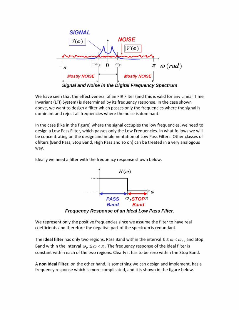
In the typical filtering problem we want to separate a signal from an additive disturbance. In general within the frequency spectrum we can see frequencies in which the signal is dominant and frequencies where the noise is dominant. This is shown in the figure below.
Signal and Noise in the Digital Frequency Spectrum
We have seen that the effectiveness of an FIR Filter (and this is valid for any Linear Time Invariant (LTI) System) is determined by its frequency response. In the case shown above, we want to design a filter which passes only the frequencies where the signal is dominant and reject all frequencies where the noise is dominant. In the case (like in the figure) where the signal occupies the low frequencies, we need to design a Low Pass Filter, which passes only the Low Frequencies. In what follows we will be concentrating on the design and implementation of Low Pass Filters. Other classes of dfilters (Band Pass, Stop Band, High Pass and so on) can be treated in a very analogous way. Ideally we need a filter with the frequency response shown below.
Frequency Response of an Ideal Low Pass Filter.
We represent only the positive frequencies since we assume the filter to have real coefficients and therefore the negative part of the spectrum is redundant. The ideal filter has only two regions: Pass Band within the interval Pωω <≤0 , and Stop Band within the interval πωω <≤P . The frequency response of the ideal filter is constant within each of the two regions. Clearly it has to be zero within the Stop Band. A non Ideal Filter, on the other hand, is something we can design and implement, has a frequency response which is more complicated, and it is shown in the figure below.
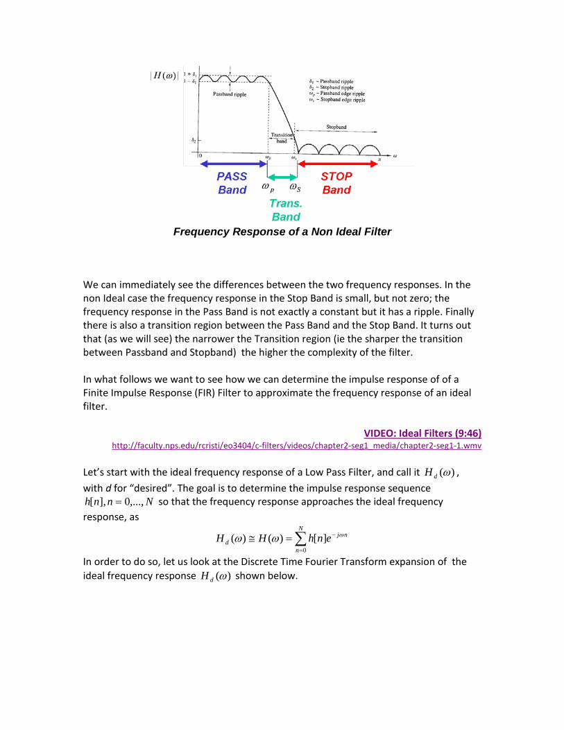
Frequency Response of a Non Ideal Filter
We can immediately see the differences between the two frequency responses. In the non Ideal case the frequency response in the Stop Band is small, but not zero; the frequency response in the Pass Band is not exactly a constant but it has a ripple. Finally there is also a transition region between the Pass Band and the Stop Band. It turns out that (as we will see) the narrower the Transition region (ie the sharper the transition between Passband and Stopband) the higher the complexity of the filter. In what follows we want to see how we can determine the impulse response of of a Finite Impulse Response (FIR) Filter to approximate the frequency response of an ideal filter.
Let’s start with the ideal frequency response of a Low Pass Filter, and call it )(ωdH , with d for “desired”. The goal is to determine the impulse response sequence
Nnnh ,...,0],[ = so that the frequency response approaches the ideal frequency response, as
∑=
−=≅N
n
njd enhHH
0][)()( ωωω
In order to do so, let us look at the Discrete Time Fourier Transform expansion of the ideal frequency response )(ωdH shown below.
Then, by the DTFT, we can find an infinite sequence +∞−∞= ,...,],[ nnhd such that
{ } ∑+∞
−∞=
−==n
njddd enhnhDTFTH ωω ][][)(
This sequence is computed by the Inverse DTFT (IDTFT) as
{ } ∫+
−
==π
π
ω ωωπ
ω deHHIDTFTnh njddd )(
21)(][
Substitute for )(ωdH as in the figure above and we obtain
( )
=== ∫
+
−
nn
ndenh PPPnjd
P
Pπω
πω
πωω
π
ω
ω
ω sincsin21][
where we define
( )x
xxππ )sin(sinc =
A plot of ][nhd with 4/πω =P is shown in the figure below.
Impulse response of Ideal Low Pass Filter (Pass Band 4/πω =P )
VIDEO: Non Ideal Filters (7:51) http://faculty.nps.edu/rcristi/eo3404/c-filters/videos/chapter2-seg1_media/chapter2-seg1-2.wmv
Now notice the following. As ±∞→n , 0][ →nhd , which means that the coefficients get smaller and smaller. Then we can use only the dominant values, say
][],...,[ LhLh dd − , with L a chosen parameter, to approximate the ideal filter as
∑+
−=
−≅L
Ln
njdd enhH ωω ][)(
Now let the filter impulse response be defined as
][][ Lnhnh d −=
Then the frequency response of the filter we obtain is the following
Ljd
LjL
Ln
njd
L
n
njd
L
n
nj
eHeenh
eLnhenhH
ωωω
ωω
ω
ω
−−
−=
−
=
−
=
−
≅
=
−==
∑
∑∑
)(][
][][)(2
0
2
0
This means that magnitude and phase of the FIR filter are related to the ideal as
passband the within )()()(
LHHH d
ωω
ωω
−=∠
≅
The last expression on the phase is valid within the passband where the phase of the ideal filter is zero. Finally choose the impulse response of the FIR filter as
NnLnLnhnh PPd ,...,0,)(sinc][][ =
−=−=πω
πω
where .2LN = See an example.
VIDEO: Example using Matlab (7.44) http://faculty.nps.edu/rcristi/eo3404/c-filters/videos/chapter2-seg1_media/chapter2-seg1-3.wmv
Example. We want design a Low Pass Filter with Pass Band 4/πω =P radians and order
40=N . Then 20=L and we obtain the impulse response
N=40; % Filter Order. It has to be even L=N/2; % time delay n=0:N; % generate the vector of time indeces h=(1/4)*sinc((n-20)/4); % Impulse response freqz(h,1) % show frequency response The plot of the frequency response is shown in the figure below. Notice two things: a. the filter is Low Pass, in the sense that it passes the low frequencies and it attenuates the high frequencies. This can be seen from the magnitude plot, showing a bandwidth of
πω 25.0= as expected; b. the phase within the passband (ie in the interval πω 25.00 << ) is linear as Lω− with 20=L .
Frequency Response of the Filter in the Example
Notice that the attenuation in the stopband is not more than 20dB, in general not very acceptable. Since we are truncating the impulse response abruptly, we create high frequency components in the frequency response of the filter, which is responsible for the poor attenuation of the filter in the stopband. Following an approach similar to what we did with the DFT, where we were trying to lower the sidelobes of the frequency spectrum, we can improve the response in the stopband by smoothing the impulse response with a window.
VIDEO: Filter Design using a Window (7:06) http://faculty.nps.edu/rcristi/eo3404/c-filters/videos/chapter2-seg1_media/chapter2-seg1-4.wmv
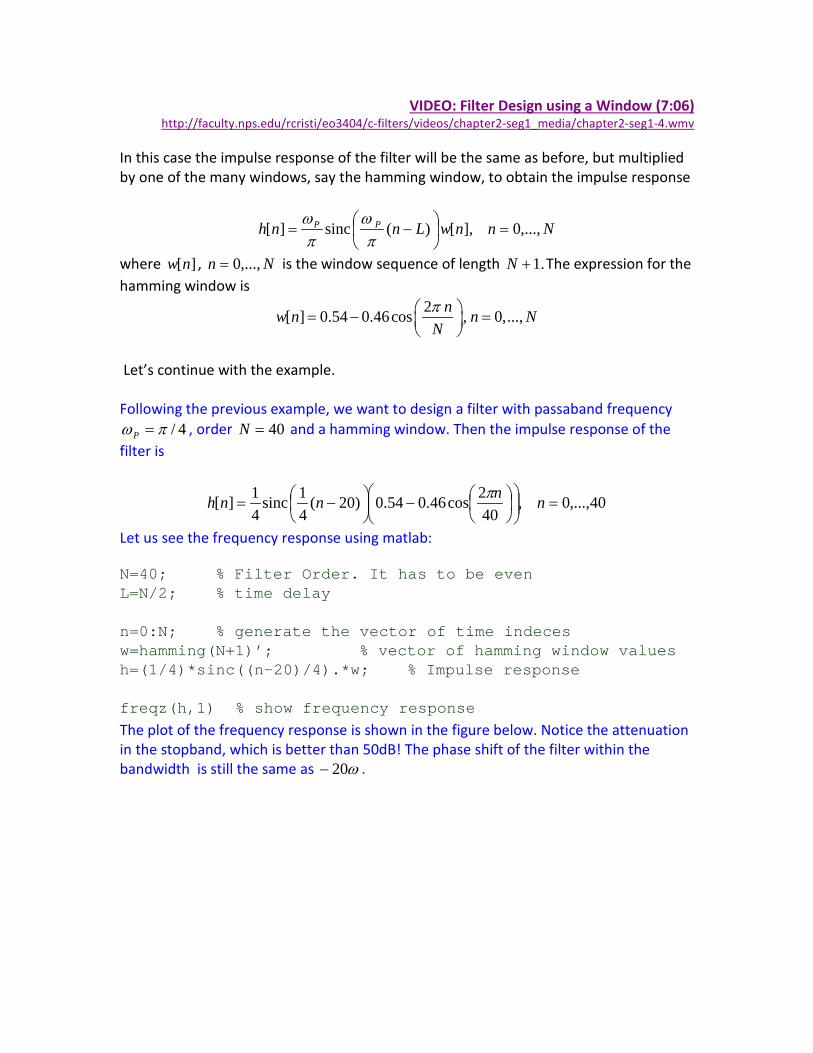
In this case the impulse response of the filter will be the same as before, but multiplied by one of the many windows, say the hamming window, to obtain the impulse response
NnnwLnnh PP ,...,0],[)(sinc][ =
−=πω
πω
where ][nw , Nn ,...,0= is the window sequence of length .1+N The expression for the hamming window is
2[ ] 0.54 0.46cos , 0,...,nw n n NNπ = − =
Let’s continue with the example. Following the previous example, we want to design a filter with passaband frequency
4/πω =P , order 40=N and a hamming window. Then the impulse response of the filter is
40,...,0,402cos46.054.0)20(
41sinc
41][ =
−
−= nnnnh π
Let us see the frequency response using matlab: N=40; % Filter Order. It has to be even L=N/2; % time delay n=0:N; % generate the vector of time indeces w=hamming(N+1)’; % vector of hamming window values h=(1/4)*sinc((n-20)/4).*w; % Impulse response freqz(h,1) % show frequency response The plot of the frequency response is shown in the figure below. Notice the attenuation in the stopband, which is better than 50dB! The phase shift of the filter within the bandwidth is still the same as ω20− .
The impulse response of this filter is shown below. If you compare with the impulse response without window, notice that the window forces the impulse response to become small (close to zero) at the edges ( 0=n and Nn = ) . This gives a smooth transition from the values outside the interval, when it is forced to be zero and the values inside the interval of definition.
Impulse Response with Hamming Window.
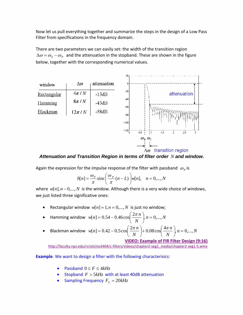
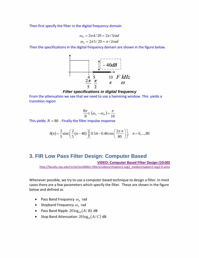
Now let us pull everything together and summarize the steps in the design of a Low Pass Filter from specifications in the frequency domain. There are two parameters we can easily set: the width of the transition region
PS ωωω −=∆ and the attenuation in the stopband. These are shown in the figure below, together with the corresponding numerical values.
Attenuation and Transition Region in terms of filter order N and window.
Again the expression for the impulse response of the filter with passband Pω is
NnnwLnnh PP ,...,0],[)(sinc][ =
−=πω
πω
where Nnnw ,...,0],[ − is the window. Although there is a very wide choice of windows, we just listed three significative ones:
• Rectangular window Nnnw ,...,0,1][ == is just no window;
• Hamming window NnN
nnw ,...,0,2cos46.054.0][ =
−=π
• Blackman window NnN
nN
nnw ,...,0,4cos08.02cos5.042.0][ =
+
−=
ππ
VIDEO: Example of FIR Filter Design (9:16) http://faculty.nps.edu/rcristi/eo3404/c-filters/videos/chapter2-seg1_media/chapter2-seg1-5.wmv
Example. We want to design a filter with the following characterisics:
• Passband kHzF 40 ≤≤ • Stopband kHzF 5> with at least 40dB attenuation • Sampling Frequency kHzFS 20=
Whenever possible, we try to use a computer based technique to design a filter. In most cases there are a few parameters which specify the filter. These are shown in the figure below and defined as
• Pass Band Frequency Pω rad • Stopband Frequency Sω rad • Pass Band Ripple )/(log20 10 BA dB • Stop Band Attenuation ( )CA /log20 10 dB
As we can easily see, these parameters attempt to quantify how close to “ideal” is the frequency response of a filter. One of the most effective designs of digital filters is the “equiripple filter”, which is shown to be the one with the smallest maximum deviation from ideal. It requires a computerized algorithm which, in recent versions of Matlab, goes under the name of “firpm”, with “pm” standing for Parks and MacClellan, the designers. The same algorithm in older versions was called “remez”, with very similar parametrization. The first step in the design is to specify the desired filter (say a Low Pass Filter, but it can be any kind of filter) by a set of parameters. Referring to the figure below, the filter is specified by pairs of points of the frequency response.
Specification of Ideal Low Pass Filter parameters
Referring to the figure, given the four points, the ideal filter we want to approximate is determined by linear interpolation of each pair. Before going into more details, notice that the number of points has to be even, since the segments have to be disjoint. The reason is a bit like “give and take”. If you want to have a real good approximation in specific regions of interest (in the passband PASSω→0 and the stopband πω →STOP ) you need to leave it “loose” in regions of less interest (the transition region
STOPPASS ωω → ). If we constrain it too much, by specifying what we want even within the transition region, we end up with an unsatisfactory design. Again following the figure above, we see that the filter is specified by two vectors, one specifying the amplitudes
A=[1,1,0,0] and one specifying the frequencies defined as πω /=f as f=[0,f1,f2,1]
where πω /f1 PASS= and πω /f2 STOP= . Then we need to specify the filter order N, which can be done on the basis of an empirical formula which relates it to the desired attenuation of the filter, as
πωω /11(dB) A~
PASSSTOP
ttenuationN−×
Finally, using these parameters, we use the function “firpm” to determine the impulse response of the filter: h=firpm(N,f,A); The vector “h” yields the impulse response of the filter as
[ ]][]1[],0[ Nhhhh = Let’s see and example.
VIDEO: Low Pass Filter Design Example (5:44) http://faculty.nps.edu/rcristi/eo3404/c-filters/videos/chapter2-seg2_media/chapter2-seg2-1.wmv
Example.We want to design a digital Low Pass Filter with the following specifications: Passband frequencies: up to 3.0 kHz Stopband frequencies: above 3.5 kHz Attenuation in Stopband: 60 dB Sampling Frequency: 15.0 kHz The first step is the specification of the filter in terms of digital frequencies
SFF /2πω = :
157
000,15500,32
52
000,15000,32
ππω
ππω
==
==
STOP
PASS
Then we determine an estimate of the order of the filter
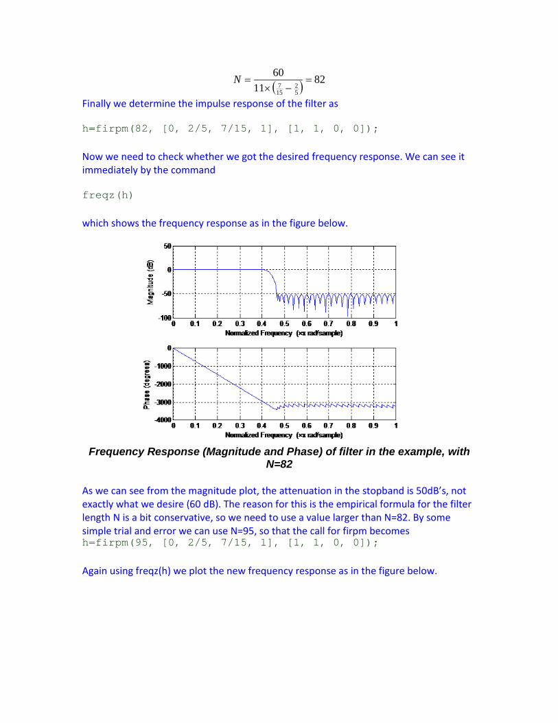
Finally we determine the impulse response of the filter as h=firpm(82, [0, 2/5, 7/15, 1], [1, 1, 0, 0]); Now we need to check whether we got the desired frequency response. We can see it immediately by the command freqz(h) which shows the frequency response as in the figure below.
Frequency Response (Magnitude and Phase) of filter in the example, with
N=82 As we can see from the magnitude plot, the attenuation in the stopband is 50dB’s, not exactly what we desire (60 dB). The reason for this is the empirical formula for the filter length N is a bit conservative, so we need to use a value larger than N=82. By some simple trial and error we can use N=95, so that the call for firpm becomes h=firpm(95, [0, 2/5, 7/15, 1], [1, 1, 0, 0]); Again using freqz(h) we plot the new frequency response as in the figure below.
0 0.1 0.2 0.3 0.4 0.5 0.6 0.7 0.8 0.9 1-4000
-3000
-2000
-1000
0
Normalized Frequency (×π rad/sample)
Pha
se (d
egre
es)
0 0.1 0.2 0.3 0.4 0.5 0.6 0.7 0.8 0.9 1-100
-50
0
50
Normalized Frequency (×π rad/sample)
Mag
nitu
de (d
B)
Frequency Response of filter in the same example, with N=95
Looking at the magnitude plot, we se that the attenuation is about 60dB as we require from the design specifications. The impulse of the filter can be plotted by stem(h) and it is shown in the figure below.
Impulse Response of filter in the example
4. Example of Application VIDEO: Example of Application (9:38)
In a number of applications, such as in Radar, Sonar and Communications, we transmit information through a pulse or a sequence of pulses. At the receiver the signal is attenuated by the propagation within the medium in between (say air, space or water) and corrupted by disturbances and noise. The first step at the receiver will be to try to eliminate some of the disturbances before processing. For example suppose we transmit a pulse made of four periods of a sinusoid as
010 40),2sin()( TTttFAtx =≤≤= π where the frequency 0F and length in time 1T are given by
sec8sec500
14
500
1
0
mT
HzF
=×=
=
The signal is plotted in the figure below.
Transmitted Pulse )(tx in the example
For example for a communication signal we send a binary message made of “zeros” and “ones” with (say) the following assignment
)(0)(1tx
tx−→
→
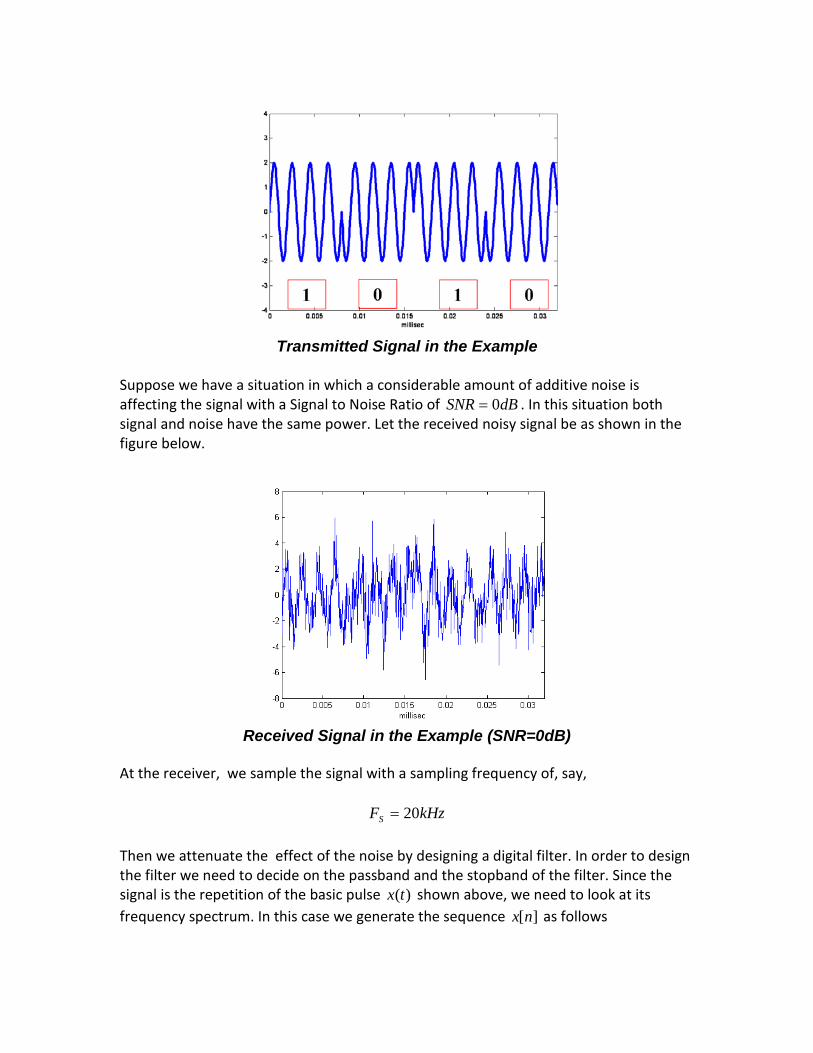
In this case a transmitted sequence “ 1 0 1 0 “ would look yield the signal shown in the figure below.
Suppose we have a situation in which a considerable amount of additive noise is affecting the signal with a Signal to Noise Ratio of dBSNR 0= . In this situation both signal and noise have the same power. Let the received noisy signal be as shown in the figure below.
Received Signal in the Example (SNR=0dB)
At the receiver, we sample the signal with a sampling frequency of, say,
kHzFS 20= Then we attenuate the effect of the noise by designing a digital filter. In order to design the filter we need to decide on the passband and the stopband of the filter. Since the signal is the repetition of the basic pulse )(tx shown above, we need to look at its frequency spectrum. In this case we generate the sequence ][nx as follows
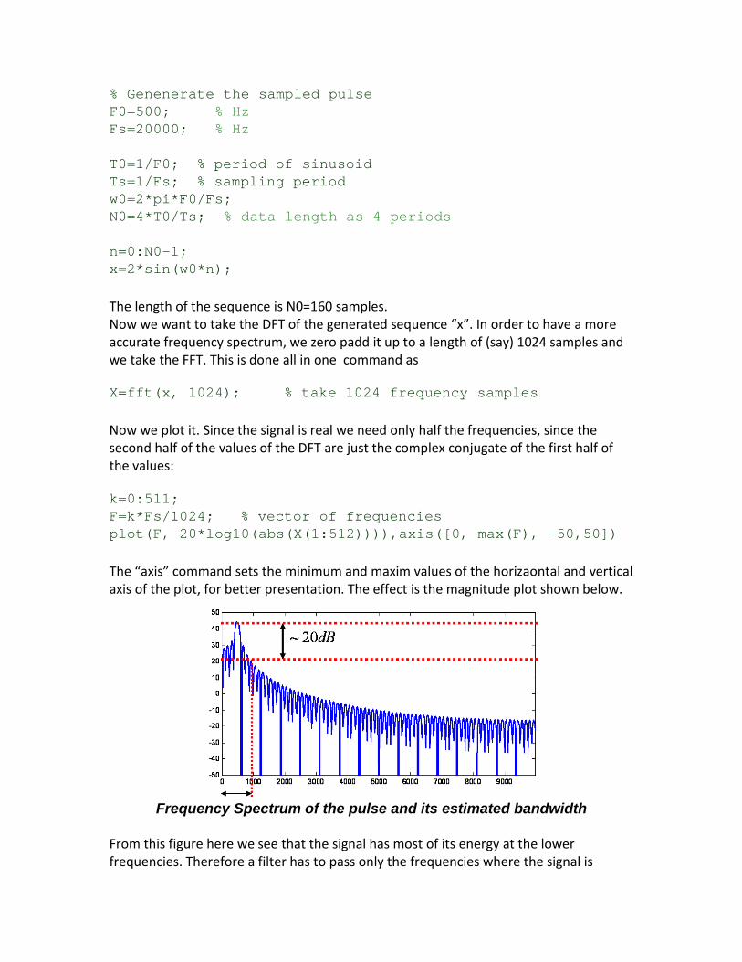
% Genenerate the sampled pulse F0=500; % Hz Fs=20000; % Hz T0=1/F0; % period of sinusoid Ts=1/Fs; % sampling period w0=2*pi*F0/Fs; N0=4*T0/Ts; % data length as 4 periods n=0:N0-1; x=2*sin(w0*n); The length of the sequence is N0=160 samples. Now we want to take the DFT of the generated sequence “x”. In order to have a more accurate frequency spectrum, we zero padd it up to a length of (say) 1024 samples and we take the FFT. This is done all in one command as X=fft(x, 1024); % take 1024 frequency samples Now we plot it. Since the signal is real we need only half the frequencies, since the second half of the values of the DFT are just the complex conjugate of the first half of the values: k=0:511; F=k*Fs/1024; % vector of frequencies plot(F, 20*log10(abs(X(1:512)))),axis([0, max(F), -50,50]) The “axis” command sets the minimum and maxim values of the horizaontal and vertical axis of the plot, for better presentation. The effect is the magnitude plot shown below.
Frequency Spectrum of the pulse and its estimated bandwidth
From this figure here we see that the signal has most of its energy at the lower frequencies. Therefore a filter has to pass only the frequencies where the signal is
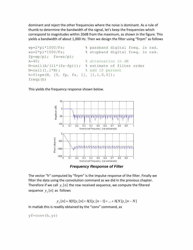
dominant and reject the other frequencies where the noise is dominant. As a rule of thumb to determine the bandwidth of the signal, let’s keep the frequencies which correspond to magnitudes within 20dB from the maximum, as shown in the figure. This yields a bandwidth of about 1,000 Hz. Then we design the filter using “firpm” as follows wp=2*pi*1000/Fs; % passband digital freq. in rad. ws=2*pi*1500/Fs; % stopband digital freq. in rad. fp=wp/pi; fs=ws/pi; A=40; % attenuation in dB N=ceil(A/(11*(fs-fp))); % estimate of filter order N=ceil(1.1*N); % add 10 percent h=firpm(N, [0, fp, fs, 1], [1,1,0,0]); freqz(h) This yields the frequency response shown below.
Frequency Response of Filter
The vector “h” computed by “firpm” is the impulse response of the filter. Finally we filter the data using the convolution command as we did in the previous chapter. Therefore if we call ][nyr the row received sequence, we compute the filtered sequence ][ny f as follows
][][...]1[]1[][]0[][ NnyNhnyhnyhny rrrf −++−+= In matlab this is readily obtained by the “conv” command, as yf=conv(h,yr)
This yields the sequence shown in the figure below, compared with the received sequence.
Top: received noisy sequence
Bottom: sequence after the filter Comparing the filtered sequence with the original transmitted sequence we see that a good amount of noise has been eliminated by the filter.


![Jan Beutel, ETH Zurich - Welcome - TIK...[B. Jelk] High‐resolution TimelapsePhotography 2009 C2 2010 C2 2011 C2 2012 C2 2013 C2 2014 C2 18.05.2015 C2 19.05.2015 C2 29.05.2015 C2](https://static.documents.pub/doc/80x56/60110b99540db573571546c3/jan-beutel-eth-zurich-welcome-tik-b-jelk-higharesolution-timelapsephotography.jpg)

