37
General Relativity Lecture Notes C348 c Mitchell A Berger Mathematics University College London 2004
| Date post: | 31-Mar-2016 |
| Category: |
Documents |
| Upload: | ucaptd-three |
| View: | 252 times |
| Download: | 1 times |

General Relativity
Lecture Notes C348
c© Mitchell A BergerMathematics University College London 2004
Contents
1 Manifolds, Vectors, and Gradients 11.1 Manifolds . . . . . . . . . . . . . . . . . . . . . . . . . . . . . . . . . . . . . . . . 1
1.1.1 Product Manifolds . . . . . . . . . . . . . . . . . . . . . . . . . . . . . . . 41.2 Co-ordinate Transformations . . . . . . . . . . . . . . . . . . . . . . . . . . . . . 51.3 Things that Live on Manifolds . . . . . . . . . . . . . . . . . . . . . . . . . . . . 5
1.3.1 Scalar fields . . . . . . . . . . . . . . . . . . . . . . . . . . . . . . . . . . . 51.3.2 Curves . . . . . . . . . . . . . . . . . . . . . . . . . . . . . . . . . . . . . . 51.3.3 Parametrized Surfaces . . . . . . . . . . . . . . . . . . . . . . . . . . . . . 61.3.4 Vectors . . . . . . . . . . . . . . . . . . . . . . . . . . . . . . . . . . . . . 71.3.5 Gradients . . . . . . . . . . . . . . . . . . . . . . . . . . . . . . . . . . . . 8
1.4 Transformation Laws . . . . . . . . . . . . . . . . . . . . . . . . . . . . . . . . . . 91.4.1 Vectors . . . . . . . . . . . . . . . . . . . . . . . . . . . . . . . . . . . . . 91.4.2 Gradients . . . . . . . . . . . . . . . . . . . . . . . . . . . . . . . . . . . . 91.4.3 Notation . . . . . . . . . . . . . . . . . . . . . . . . . . . . . . . . . . . . . 10
1.5 Duality between Vectors and Gradients . . . . . . . . . . . . . . . . . . . . . . . 141.5.1 The directional derivative . . . . . . . . . . . . . . . . . . . . . . . . . . . 141.5.2 Invariance . . . . . . . . . . . . . . . . . . . . . . . . . . . . . . . . . . . . 151.5.3 Geometric Interpretation . . . . . . . . . . . . . . . . . . . . . . . . . . . 15
2 Tensors and Metrics 162.1 Tensors . . . . . . . . . . . . . . . . . . . . . . . . . . . . . . . . . . . . . . . . . 162.2 Getting the transformation correct . . . . . . . . . . . . . . . . . . . . . . . . . . 172.3 Things to do with tensors . . . . . . . . . . . . . . . . . . . . . . . . . . . . . . . 182.4 The Levi–Civita Tensor . . . . . . . . . . . . . . . . . . . . . . . . . . . . . . . . 20
2.4.1 Odd / Even Permutations . . . . . . . . . . . . . . . . . . . . . . . . . . . 212.5 3-Vector Identities . . . . . . . . . . . . . . . . . . . . . . . . . . . . . . . . . . . 212.6 Metrics . . . . . . . . . . . . . . . . . . . . . . . . . . . . . . . . . . . . . . . . . 232.7 Euclidean Metrics . . . . . . . . . . . . . . . . . . . . . . . . . . . . . . . . . . . 24
2.7.1 E3 Euclidean 3-space . . . . . . . . . . . . . . . . . . . . . . . . . . . . . 252.7.2 E3: Cylindrical Co-ordinates . . . . . . . . . . . . . . . . . . . . . . . . . 26
2.8 Arc Length . . . . . . . . . . . . . . . . . . . . . . . . . . . . . . . . . . . . . . . 262.9 Scalar Product and Magnitude for Vectors . . . . . . . . . . . . . . . . . . . . . . 272.10 Raising and Lowering Operators . . . . . . . . . . . . . . . . . . . . . . . . . . . 282.11 Signature of the Metric . . . . . . . . . . . . . . . . . . . . . . . . . . . . . . . . 292.12 Riemannian and Pseudo-Riemannian metrics . . . . . . . . . . . . . . . . . . . . 29
i
2.13 Map Projections . . . . . . . . . . . . . . . . . . . . . . . . . . . . . . . . . . . . 302.13.1 Cylindrical Map . . . . . . . . . . . . . . . . . . . . . . . . . . . . . . . . 302.13.2 Mercator Projection . . . . . . . . . . . . . . . . . . . . . . . . . . . . . . 31
3 Special Relativity 343.1 Minkowski Space-time . . . . . . . . . . . . . . . . . . . . . . . . . . . . . . . . . 343.2 Units . . . . . . . . . . . . . . . . . . . . . . . . . . . . . . . . . . . . . . . . . . . 353.3 Einstein’s Axioms of Special Relativity . . . . . . . . . . . . . . . . . . . . . . . . 373.4 Space-Time Diagrams . . . . . . . . . . . . . . . . . . . . . . . . . . . . . . . . . 373.5 The Poincare and Lorentz Groups . . . . . . . . . . . . . . . . . . . . . . . . . . 41
3.5.1 Group Axioms . . . . . . . . . . . . . . . . . . . . . . . . . . . . . . . . . 423.6 Lorentz Boosts . . . . . . . . . . . . . . . . . . . . . . . . . . . . . . . . . . . . . 43
3.6.1 Deriving the transformation matrix . . . . . . . . . . . . . . . . . . . . . . 433.7 Simultaneity . . . . . . . . . . . . . . . . . . . . . . . . . . . . . . . . . . . . . . . 463.8 Length Contraction . . . . . . . . . . . . . . . . . . . . . . . . . . . . . . . . . . . 463.9 Relativistic Dynamics . . . . . . . . . . . . . . . . . . . . . . . . . . . . . . . . . 48
3.9.1 The 4-momentum . . . . . . . . . . . . . . . . . . . . . . . . . . . . . . . 483.9.2 Forces . . . . . . . . . . . . . . . . . . . . . . . . . . . . . . . . . . . . . . 493.9.3 Energy-Momentum Conservation . . . . . . . . . . . . . . . . . . . . . . . 503.9.4 Photons . . . . . . . . . . . . . . . . . . . . . . . . . . . . . . . . . . . . . 50
4 Maxwell’s Equations in Tensor Form 524.1 Maxwell’s Equations – Review . . . . . . . . . . . . . . . . . . . . . . . . . . . . 52
4.1.1 Internal Structure Equations . . . . . . . . . . . . . . . . . . . . . . . . . 524.1.2 Source Equations . . . . . . . . . . . . . . . . . . . . . . . . . . . . . . . . 534.1.3 Lorentz Force . . . . . . . . . . . . . . . . . . . . . . . . . . . . . . . . . . 544.1.4 Charge Conservation . . . . . . . . . . . . . . . . . . . . . . . . . . . . . . 54
4.2 The Faraday Tensor . . . . . . . . . . . . . . . . . . . . . . . . . . . . . . . . . . 554.3 Internal Structure Equations . . . . . . . . . . . . . . . . . . . . . . . . . . . . . 554.4 Source Equations . . . . . . . . . . . . . . . . . . . . . . . . . . . . . . . . . . . . 564.5 Charge Conservation . . . . . . . . . . . . . . . . . . . . . . . . . . . . . . . . . . 574.6 Lorentz Force . . . . . . . . . . . . . . . . . . . . . . . . . . . . . . . . . . . . . . 574.7 Potential Form . . . . . . . . . . . . . . . . . . . . . . . . . . . . . . . . . . . . . 58
4.7.1 Advantage – Internal Structure Equations . . . . . . . . . . . . . . . . . . 584.7.2 Advantage – Source Equations . . . . . . . . . . . . . . . . . . . . . . . . 58
4.8 Gauge Transformations . . . . . . . . . . . . . . . . . . . . . . . . . . . . . . . . 594.9 Lorentz Gauge . . . . . . . . . . . . . . . . . . . . . . . . . . . . . . . . . . . . . 594.10 Light Waves . . . . . . . . . . . . . . . . . . . . . . . . . . . . . . . . . . . . . . . 60
5 The Equivalence Principle 625.1 Inertial mass . . . . . . . . . . . . . . . . . . . . . . . . . . . . . . . . . . . . . . 625.2 Free Fall . . . . . . . . . . . . . . . . . . . . . . . . . . . . . . . . . . . . . . . . . 63
5.2.1 Locally Inertial Frames . . . . . . . . . . . . . . . . . . . . . . . . . . . . 645.3 Geodesics . . . . . . . . . . . . . . . . . . . . . . . . . . . . . . . . . . . . . . . . 64
5.3.1 Examples . . . . . . . . . . . . . . . . . . . . . . . . . . . . . . . . . . . . 655.3.2 The Geodesic Equation . . . . . . . . . . . . . . . . . . . . . . . . . . . . 65
ii

5.3.3 Covariant Acceleration . . . . . . . . . . . . . . . . . . . . . . . . . . . . . 67
6 Covariant Derivatives 696.1 Non-Euclidean Geometry . . . . . . . . . . . . . . . . . . . . . . . . . . . . . . . 696.2 The Covariant Derivative . . . . . . . . . . . . . . . . . . . . . . . . . . . . . . . 716.3 Derivatives of Other Tensors . . . . . . . . . . . . . . . . . . . . . . . . . . . . . 72
6.3.1 The gradient of the metric in General Relativity . . . . . . . . . . . . . . 746.4 Covariant Directional Derivatives and Acceleration . . . . . . . . . . . . . . . . . 746.5 Newton’s Law of motion . . . . . . . . . . . . . . . . . . . . . . . . . . . . . . . . 756.6 Twin Paradox . . . . . . . . . . . . . . . . . . . . . . . . . . . . . . . . . . . . . . 76
6.6.1 The rapidity . . . . . . . . . . . . . . . . . . . . . . . . . . . . . . . . . . 77
7 Orbits 797.1 Noether’s Theorem . . . . . . . . . . . . . . . . . . . . . . . . . . . . . . . . . . . 797.2 The Schwarzschild Metric . . . . . . . . . . . . . . . . . . . . . . . . . . . . . . . 80
7.2.1 Symmetries and Conserved Quantities . . . . . . . . . . . . . . . . . . . . 817.2.2 Orbits in the Equatorial Plane . . . . . . . . . . . . . . . . . . . . . . . . 82
7.3 Precession of Mercury’s Orbit . . . . . . . . . . . . . . . . . . . . . . . . . . . . . 857.3.1 Method . . . . . . . . . . . . . . . . . . . . . . . . . . . . . . . . . . . . . 867.3.2 Newtonian Solution . . . . . . . . . . . . . . . . . . . . . . . . . . . . . . 877.3.3 Relativistic Correction . . . . . . . . . . . . . . . . . . . . . . . . . . . . . 88
7.4 Deflection of Starlight . . . . . . . . . . . . . . . . . . . . . . . . . . . . . . . . . 897.4.1 Newtonian Theory . . . . . . . . . . . . . . . . . . . . . . . . . . . . . . . 897.4.2 Relativistic Theory . . . . . . . . . . . . . . . . . . . . . . . . . . . . . . . 90
7.5 Energy Conservation on Geodesics . . . . . . . . . . . . . . . . . . . . . . . . . . 92
iii

Chapter 1
Manifolds, Vectors, and Gradients
... ‘You must follow me carefully. I shall have to controvert one or two ideas that are almost universallyaccepted. The geometry, for instance, they taught you at school is founded on a misconception.’
‘Is not that rather a large thing to expect us to begin upon?’ said Filby ....The Time Machine, HG Wells 1895
1.1 Manifolds
Mathematics provides a common mathematical term for curved surfaces, curved spaces, and evencurved space-times – the manifold. In essence, a manifold is an N-Dimensional surface. Thismeans that each point of the manifold can be located by specifying N numbers or coordinates.More formally,
Definition 1.1 Manifold
• A manifold M is a set of points which can locally be mapped into RN for some N =0, 1, 2, . . . . The number N will be called the dimension of the manifold.
• The mapping must be one-to-one.
• If two mappings overlap, one must be a differentiable function of the other.
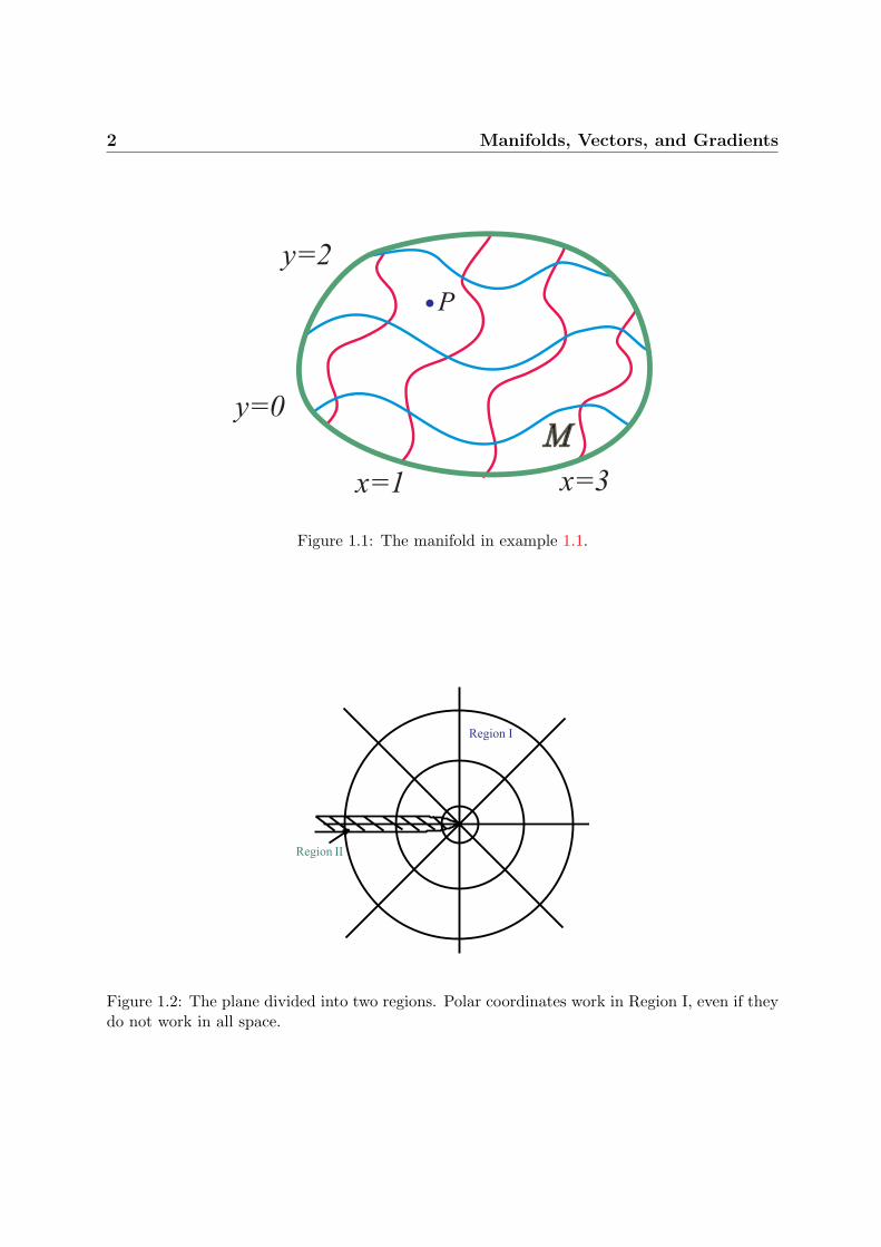
Example 1.1 Let M be a two dimensional surface. Suppose we have a point P and we wishto say where this point is. We can do this by specifying two coordinates x and y for P . In figure1.1 P is mapped to (x, y) = (0.5, 1.5), i.e. P is given the co-ordinates (0.5, 1.5). Note that thelines of constant x never cross each other (similarly for the lines of constant y) – if they did,then the coordinates of the crossing point would not be unique.
Example 1.2 Suppose we try to map the same surface M using polar coordinates r and φ.Here we run into difficulties:
• The φ function is not single-valued (one-to-one) at r = 0. Any coordinate pair (r, φ) =(0, φ) refers to the origin.
• The mapping is not continuous for all values of φ as angles only have a range of 2π. – wemust cut the plane, say at the φ = π or − π line. Then φ will not be continuous acrossthis line.
1
2 Manifolds, Vectors, and Gradients
Figure 1.1: The manifold in example 1.1.
Figure 1.2: The plane divided into two regions. Polar coordinates work in Region I, even if theydo not work in all space.

1.1 Manifolds 3
Figure 1.3: Spherical coordinates.
Note that polars are still well-defined in regions which avoid the origin and the cut. In thefigure, polar coordinates are single valued and continuous in region I, but not in the entire plane.We remedy the situation by using a different co-ordinate system in region II. (For example, wecould employ Cartesian coordinates in region II.)
Example 1.3 M = S1 (circle). There is one coordinate φ which can be chosen to go from−π to π. The point mapped to φ = π also maps to φ = −π. Thus we will need at least twoco-ordinate patches.
To summarize: we cover a manifold M with co-ordinate patches. In each patch, the coordi-nates form a cross-hatch. The minimum number of patches needed depends on the topology ofM . In the previous example, M = S1 needs two patches. A manifold M = R2 consisting of theentire plane needs only one (using Cartesian coordinates rather than polars).
Example 1.4 The 2-sphereM = S2. Spherical coordinates do not cover the entire sphere in aone-to-one continuous fashion; azimuthal angle φ is many-valued at the poles and is discontinuousat φ = ±π. On a globe of the Earth, φ corresponds to longitude, which is discontinuous at theinternational date line drawn near (±180o).
Exercise 1.1 Cover the 2-sphere S2 with just two coordinate patches.
Example 1.5 Sn (n-sphere)
Sn ={
(X1,X2, . . . ,Xn+1) | (X1)2 + (X2)2 + · · ·+ (Xn+1)2 = 1}
(1.1)
4 Manifolds, Vectors, and Gradients
e.g. S2 ={
(x, y, z) |x2 + y2 + z2 = 1}
S1 ={
(x, y) |x2 + y2 = 1}
S0 ={x |x2 = 1
}={−1, 1
}(1.2)
Example 1.6 Bn (n-ball)
Bn ={
(X1,X2, . . . ,Xn) | (X1)2 + (X2)2 + · · ·+ (Xn)2 < 1}
(1.3)
i.e Bn is the solid volume inside Sn−1.
1.1.1 Product Manifolds
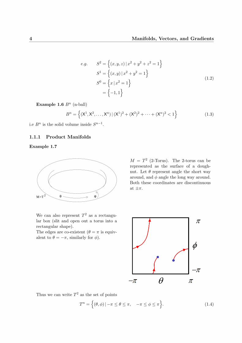
Example 1.7
=T 2M θ φ
M = T 2 (2-Torus). The 2-torus can berepresented as the surface of a dough-nut. Let θ represent angle the short wayaround, and φ angle the long way around.Both these coordinates are discontinuousat ±π.
We can also represent T 2 as a rectangu-lar box (slit and open out a torus into arectangular shape).The edges are co-existent (θ = π is equiv-alent to θ = −π, similarly for φ).
Thus we can write T 2 as the set of points
Tn ={
(θ, φ) | −π ≤ θ ≤ π, −π ≤ φ ≤ π}. (1.4)
1.2 Co-ordinate Transformations 5
Note that in the definition of T 2, the coordinates θ and φ are completely independent.By themselves, each gives a circle S1. We can express this independence with the notationT 2 = S1 × S1. We call T 2 a product manifold, as it can be generated by considering allcombinations of θ (the first S1) and φ (the second S1).
1.2 Co-ordinate Transformations
Suppose we know the coordinates of points in a manifold in one coordinate system. We mayneed to be able to find the same points in other coordinate systems as well, for various reasons.Somebody we work with may use another system, so there will be a communication problemunless we can translate between systems. Or perhaps the equations we wish to solve are easierin a different system. Also, if we know general ways of going from one system to another, wecan make sure that our solutions work independently of which particular coordinate system weuse. We will only deal with coordinate systems which are differentiable functions of each other.
Suppose point P has co-ordinates X = (X1,X2, . . . ,Xn) in one co-ordinate system, andY = (Y1,Y2, . . . ,Yn) in another. Then the co-ordinates (Y1,Y2, . . . ,Yn) must be smooth (dif-ferentiable) functions of (X1,X2, . . . ,Xn). For example,
Y1 = Y1(X1,X2, . . . ,Xn). (1.5)
Also, the co-ordinate (Jacobian) transformation matrix is
∂Ya
∂Xb, (1.6)
where a labels the row, and b labels the column in the matrix.
1.3 Things that Live on Manifolds
1.3.1 Scalar fields
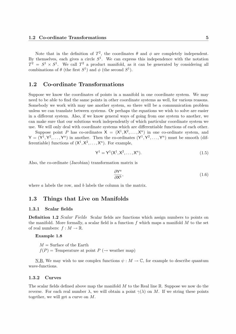
Definition 1.2 Scalar Fields Scalar fields are functions which assign numbers to points onthe manifold. More formally, a scalar field is a function f which maps a manifold M to the setof real numbers: f : M → R.
Example 1.8
M = Surface of the Earthf(P ) = Temperature at point P (→ weather map)
N.B. We may wish to use complex functions ψ : M → C, for example to describe quantumwave-functions.
1.3.2 Curves
The scalar fields defined above map the manifold M to the Real line R. Suppose we now do thereverse. For each real number λ, we will obtain a point γ(λ) on M . If we string these pointstogether, we will get a curve on M .
6 Manifolds, Vectors, and Gradients
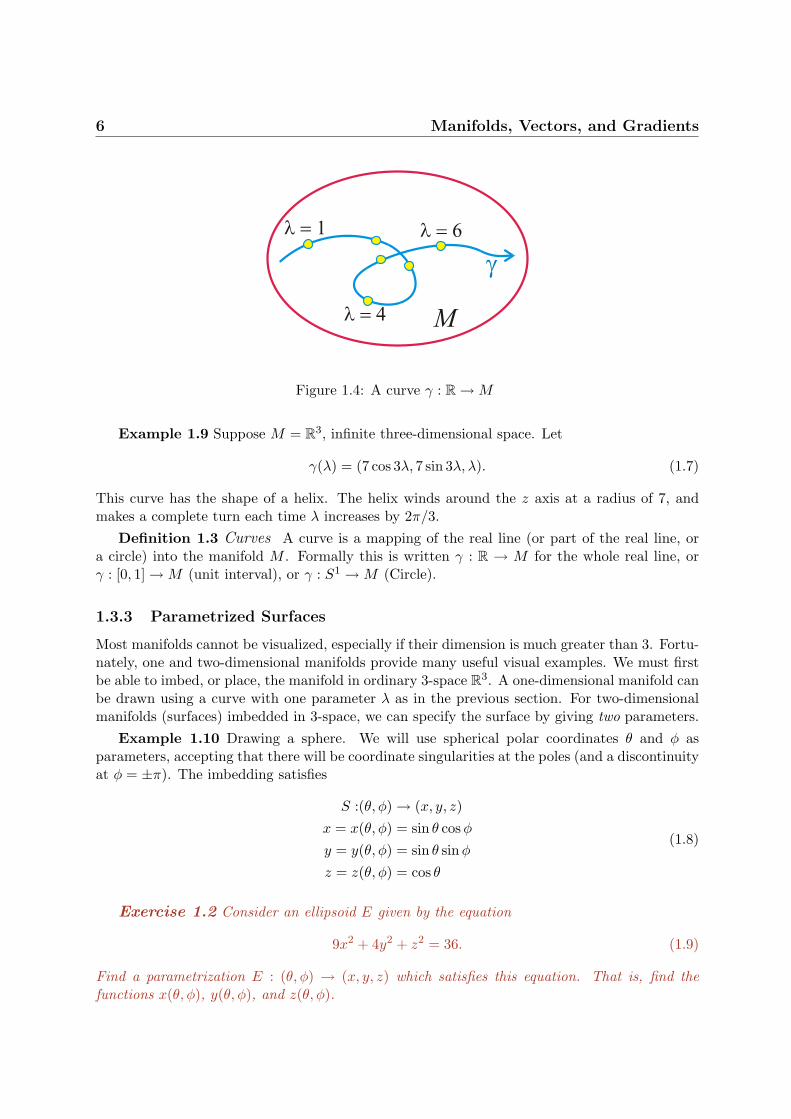
Figure 1.4: A curve γ : R →M
Example 1.9 Suppose M = R3, infinite three-dimensional space. Let
γ(λ) = (7 cos 3λ, 7 sin 3λ, λ). (1.7)
This curve has the shape of a helix. The helix winds around the z axis at a radius of 7, andmakes a complete turn each time λ increases by 2π/3.
Definition 1.3 Curves A curve is a mapping of the real line (or part of the real line, ora circle) into the manifold M . Formally this is written γ : R → M for the whole real line, orγ : [0, 1] →M (unit interval), or γ : S1 →M (Circle).
1.3.3 Parametrized Surfaces
Most manifolds cannot be visualized, especially if their dimension is much greater than 3. Fortu-nately, one and two-dimensional manifolds provide many useful visual examples. We must firstbe able to imbed, or place, the manifold in ordinary 3-space R3. A one-dimensional manifold canbe drawn using a curve with one parameter λ as in the previous section. For two-dimensionalmanifolds (surfaces) imbedded in 3-space, we can specify the surface by giving two parameters.
Example 1.10 Drawing a sphere. We will use spherical polar coordinates θ and φ asparameters, accepting that there will be coordinate singularities at the poles (and a discontinuityat φ = ±π). The imbedding satisfies
S :(θ, φ) → (x, y, z)x = x(θ, φ) = sin θ cosφy = y(θ, φ) = sin θ sinφz = z(θ, φ) = cos θ
(1.8)
Exercise 1.2 Consider an ellipsoid E given by the equation
9x2 + 4y2 + z2 = 36. (1.9)
Find a parametrization E : (θ, φ) → (x, y, z) which satisfies this equation. That is, find thefunctions x(θ, φ), y(θ, φ), and z(θ, φ).

1.3 Things that Live on Manifolds 7
Exercise 1.3 Here we find a parametrization of the Northern half of a sphere which doesnot use spherical coordinates: let the two parameters be t and u, where
S :(t, u) → (x, y, z)
x = x(t, u) = t
y = y(t, u) = u
z = z(t, u) = ?
(1.10)
Find the function z(t, u).
1.3.4 Vectors
A vector has:
• A Magnitude
• A Direction
• A Base Point
N.B. Forget “position vectors”. Position is given by co-ordinates, not by vectors. In flatEuclidean space, one can draw an arrow from the origin to any point, and in some elementarybooks this is called a vector. We will not do this, as we may wish to study highly warped man-ifolds where such arrows will also need to be warped (and hence their direction and magnitudewill not be well defined). Vectors in differential geometry always have a base point, and give adirection and magnitude proceeding from that point.
Start with a curve γ : R →M (or [0,1], or S1 →M). The curve provides a set of n coordinatefunctions of λ, i.e.
γ(λ) =(X1(λ), . . . ,Xn(λ)
). (1.11)
These n functions have derivatives which show how fast they increase with λ. Taken together,they show the direction the curve is travelling.
Definition 1.4 Tangent Vectors The tangent vector to the curve γ is given by
V(λ) =
dX1/ dλ...
dXn/ dλ
. (1.12)

8 Manifolds, Vectors, and Gradients
Note that the set of coordinates of a point (e.g. (X1, . . . ,Xn)) is not a vector!
1.3.5 Gradients
Gradients are formed from scalar functions.Definition 1.5 Gradients Given a function f : M → R,
∇f =(∂f
∂X1,∂f
∂X2, . . . ,
∂f
∂Xn
). (1.13)
This is different to a tangent vector. For one thing, it is determined everywhere on M ,whereas a tangent vector is only defined on a single curve.
Example 1.11 Consider an ordinance survey map, giving height h as a function of positionon the Earths surface h : S2 → R.
The contours are lines of constant h. But note that these are not parametrized curves! (Wehave not been given a way to choose λ = 0, 1, 2, . . . etc). Thus we have no way of definingtangent vectors to the contours (at least not until we introduce metrics, in §2.6).
Exercise 1.4 Consider a torus T2 with coordinates (X1,X2) = (u, v), where −π < u ≤ π,−π < v ≤ π. Suppose there is a curve γ : R → T2, where γ(λ) = (2πλ, 6πλ) (i.e. u(λ) = 2πλand v(λ) = 6πλ)).
Find the tangent vector
V(λ) =dγdλ.
Consider the function f(u, v) = sin(v). Find the gradient ∇f and the directional derivativeV · ∇f .
1.4 Transformation Laws 9
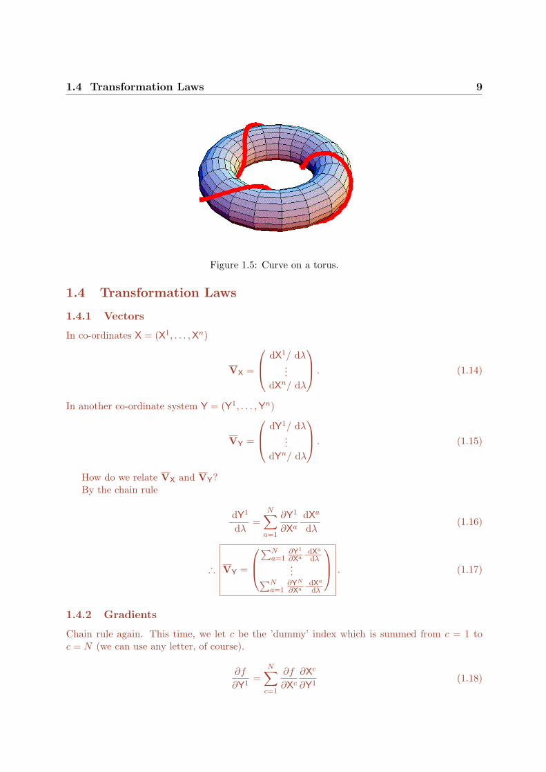
Figure 1.5: Curve on a torus.
1.4 Transformation Laws
1.4.1 Vectors
In co-ordinates X = (X1, . . . ,Xn)
VX =
dX1/ dλ...
dXn/ dλ
. (1.14)
In another co-ordinate system Y = (Y1, . . . ,Yn)
VY =
dY1/ dλ...
dYn/ dλ
. (1.15)
How do we relate VX and VY?By the chain rule
dY1
dλ=
N∑a=1
∂Y1
∂Xa
dXa
dλ(1.16)
∴ VY =
∑N
a=1∂Y1
∂XadXa
dλ...∑N
a=1∂YN
∂XadXa
dλ
. (1.17)
1.4.2 Gradients
Chain rule again. This time, we let c be the ’dummy’ index which is summed from c = 1 toc = N (we can use any letter, of course).
∂f
∂Y1=
N∑c=1
∂f
∂Xc
∂Xc
∂Y1(1.18)

10 Manifolds, Vectors, and Gradients
and so, the transformation is
∴ ∇Yf =
(N∑
c=1
∂f
∂Xc
∂Xc
∂Y1, . . . ,
N∑c=1
∂f
∂Xc
∂Xc
∂YN
). (1.19)
1.4.3 Notation
A) Einstein’s Summation Convention The placement of indices is important in geometryand relativity. The vectors we have looked at (like V 1) have been given indices on top, i.e.superscripts. Meanwhile, the gradients (like ∇1f) have indices lower down, i.e. subscripts. Thismakes it easier to distinguish between them. It also allows us to define consistent rules forcalculating inner products. But first we will simplify the notation.
In numerous expressions in geometry and relativity (and particle theory as well) there areplaces where the index a is repeated twice and summed over. If we do not bother to write downthe summation sign, then the expressions will be less cluttered.
Definition 1.6 Einstein Summation Given two objects, one indexed with superscriptsA = (A1, . . . , AN ), and one with subscripts B = (B1, . . . , BN ), we define
BcAc ≡
N∑c=1
BcAc (1.20)
In a derivative like ∂f∂Xc the index c will be considered a subscript.
Example 1.12 In the previous section, equation (1.19) becomes
∇Yf =(∂f
∂Xc
∂Xc
∂Y1, . . . ,
∂f
∂Xc
∂Xc
∂YN
). (1.21)
B) Co-ordinate system labels We will label Co-ordinate systems by either primed symbols(X′) and unprimed symbols (X), or by capital letters; for example
EarthFrame E =(E1, . . . ,EN
)Spaceship Frame S =
(S1, . . . ,SN
)LabFrame L =
(L1, . . . , LN
) (1.22)
C) Differentials∂f
∂Xa= ∂af ,
∂f
∂X′a = ∂′af ,∂f
∂Ea= ∂Eaf. (1.23)
D) Vector Components In, for example, the lab frame L the tangent vector to the curve
γ(λ) = (L1(λ), . . . , LN(λ)) (1.24)
is
V =dγdλ
=
dL1/ dλ...
dLN/ dλ
(1.25)

1.4 Transformation Laws 11
with components
V aL =
dLa
dλ. (1.26)
We sometimes refer to the whole of the vector V by referring to a typical component V a.Similarly, we may refer to ∇f as ∂af .
E) Transforms
• Vectors:
For transformations between the X frame and the Y frame, equation (1.16) becomes
V 1Y =
dY1
dλ=∂Y1
∂Xa
dXa
dλ=∂Y1
∂XaV a
X . (1.27)
The formula for an arbitrary component of V is
V bY =
∂Yb
∂XaV a
X . (1.28)
• Gradients: an arbitrary component of ∇f in equation (1.19) can now be expressed as
∂Y bf =∂Xc
∂Yb∂X cf (1.29)
• For transformations between primed and unprimed co-ordinates, these expressions become
V′b =
∂X′b
∂XaV a. (1.30)
∂′bf =∂Xc
∂X′b∂cf (1.31)
• Note that the transformation matrices in equations (1.28) and (1.29), i.e. ∂Eb/∂Sa and∂Sc/∂Eb, are inverses. Proof: The (a, c) component of the product matrix is
N∑b=1
∂Eb
∂Sa
∂Sc
∂Eb=
N∑b=1
∂Sc
∂Eb
∂Eb
∂Sa(1.32)
=∂Sc
∂Sa(1.33)
by the chain rule. But∂Sc
∂Sa=
{1 c = a
0 c 6= a(1.34)
i.e.∂Sc
∂Eb
∂Eb
∂Sa= δc
a (1.35)

12 Manifolds, Vectors, and Gradients
where
δca =
1 0 0 · · ·0 1 0 · · ·0 0 1 · · ·...
...
(1.36)
is the identity matrix. QED
This result is very important. Gradients and vectors have different (in fact, inverse)transformation laws. Thus a gradient is not a vector!
Exercise 1.5 Show that for any vector W with components W a,
δcaW
a = W c. (1.37)
• How do two successive transformations work? Suppose we transform from co-ordinatesX → Y → Z:
V aZ =
∂Za
∂YbV b
Y, where (1.38)
V bY =
∂Yb
∂XcV c
X , ⇒ (1.39)
V aZ =
∂Za
∂Yb
∂Yb
∂XcV c
X . (1.40)
But by the chain rule∂Za
∂Yb
∂Yb
∂Xc=∂Za
∂Xc(1.41)
so, (as we should expect)
V aZ =
∂Za
∂XcV c
X . (1.42)
Now try X → Y → X:
V aX =
∂Xa
∂Yb
∂Yb
∂XcV c
X (1.43)
= δacV
cX (1.44)
= V aX good! (1.45)
Example 1.13 Polar Co-ordinates.
C = (C1,C2) = (x, y) Cartesian (1.46)
P = (P1,P2) = (r, φ) Polar (1.47)
where
C1 = x = r cosφ = P1 cos P2 (1.48)
C2 = y = r sinφ = P1 sinP2 (1.49)
1.4 Transformation Laws 13
or, going the other way,
P1 = r =√x2 + y2 =
√(C1)2 + (C2)2 (1.50)
P2 = φ = arctany
x= arctan
C2
C1(1.51)
The transformation matrix (Jacobian) is:
∂Ca
∂ Pb=∂Ca
∂ Pb=(∂C1/∂P1 ∂C1/∂P2
∂C2/∂P1 ∂C2/∂P2
)(1.52)
=(∂x/∂r ∂x/∂φ∂y/∂r ∂y/∂φ
)(1.53)
=(
cosφ −r sinφsinφ r cosφ
)(1.54)
and the other way
∂Pb
∂Cd=(∂r/∂x ∂r/∂y∂φ/∂x ∂φ/∂y
)(1.55)
=(
x/r y/r−y/r2 x/r2
)(1.56)
=(
cosφ sinφ− sin φ
rcos φ
r
). (1.57)
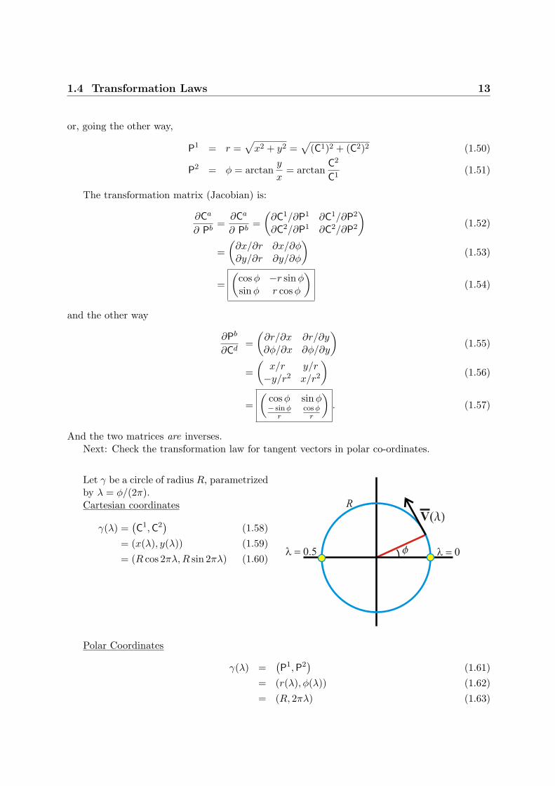
And the two matrices are inverses.Next: Check the transformation law for tangent vectors in polar co-ordinates.
Let γ be a circle of radius R, parametrizedby λ = φ/(2π).Cartesian coordinates
γ(λ) =(C1,C2
)(1.58)
= (x(λ), y(λ)) (1.59)= (R cos 2πλ,R sin 2πλ) (1.60)
Polar Coordinates
γ(λ) =(P1,P2
)(1.61)
= (r(λ), φ(λ)) (1.62)= (R, 2πλ) (1.63)

14 Manifolds, Vectors, and Gradients
The tangent vector can be computed separately for each coordinate system:Cartesian coordinates
V aC (λ) =
dCa
dλ(1.64)
=(
dx/ dλdy/ dλ
)(1.65)
=(−2πR sin 2πλ2πR cos 2πλ
). (1.66)
Polar coordinates
⇒ V aP (λ) =
dPa
dλ(1.67)
=(
dr/ dλdφ/ dλ
)(1.68)
=(
02π
). (1.69)
Let’s check the transformation law, using equation (1.54):
V aC (λ) =
∂Ca
∂PbV b
P (at r = R,φ = 2πλ) (1.70)
=(
cos 2πλ −r sin 2πλsin 2πλ r cos 2πλ
)(02π
)(1.71)
=(−2πR sin 2πλ2πR cos 2πλ
). (1.72)
IT WORKS!
1.5 Duality between Vectors and Gradients
1.5.1 The directional derivative
Two objects in maths are called ‘dual’ if they combine to give a single number (in R or C ).In elementary matrix algebra, row vectors and column vectors multiply to give a number. Inquantum theory, a bra vector 〈ψ| and a ket vector |φ〉 combine to give the complex number〈ψ|φ〉.
On a manifold, we can combine a vector, V, and a gradient, ∇f , naturally by using Einsteinsummation:
V · ∇f = V a ∂af
=N∑
a=1
V a ∂af.(1.73)
This sum gives a number called the directional derivative.Why is this ‘natural’?
1.5 Duality between Vectors and Gradients 15
1.5.2 Invariance
Exercise 1.6 Prove from the transformation laws that the directional derivative is the samein all co-ordinate systems.
Solution For the transformation from X → X′,
V a =∂Xa
∂X′bV′b
∂af =∂X
′c
∂Xa∂′cf
⇒ V · ∇f = V a∂af =
(∂Xa
∂X′b
∂X′c
∂Xa
)V′b∂′cf
= ( δcb )V
′b∂′cf
= V′c∂
′cf
(1.74)
ThusV · ∇f = V a∂af = V
′c∂′cf. (1.75)
The directional derivative has the same form in any two co-ordinate systems, and gives thesame number.
1.5.3 Geometric Interpretation
Suppose f is the temperature as a function of position. We can measure f(λ) as we travel alongγ(λ).
We can find df/ dλ by the chain rule:
dfdλ
=N∑
a=1
∂f
∂Xa
dXa
dλ
= ∂af Va
= V · ∇f.
(1.76)
In words, if the curve γ(λ) has tangent vector V, then the directional derivative V · ∇f givesthe rate of change of f along the curve, df/dλ.

Chapter 2
Tensors and Metrics
‘You know of course that a mathematical line, a line of thickness nil, has no real existence. They taughtyou that? Neither has a mathematical plane. These things are mere abstractions.’ ‘That is all right,’said the Psychologist. ‘Nor, having only length, breadth, and thickness, can a cube have a real existence.’‘There I object,’ said Filby. ‘Of course a solid body may exist. All real things’ ‘So most people think.But wait a moment. Can an instantaneous cube exist?’ ‘Dont follow you,’ said Filby. ‘Can a cube thatdoes not last for any time at all, have a real existence?’
Filby became pensive.The Time Machine, HG Wells 1895
2.1 Tensors
Tensors are classified by their rank:
Rank0 Scalars (functions) ·1 Vectors and forms (inc gradients) · · ·
2 Two indices - appear like matrices
������������������������������������
������������������������������������
������������������������������������
������������������������������������
������������������������������
������������������������������
������������������������������������
������������������������������������
������������������������������������
������������������������������������
������������������������������
������������������������������
������������������������������������
������������������������������������
������������������������������������
������������������������������������
������������������������������
������������������������������
3 Three indices - appear like a stack of matrices...
......
0th RankDefinition 2.1 Scalars A tensors with no subscripts or superscripts. They are functions of position
on the manifold, and are completely independent of coordinates.
1st RankDefinition 2.2 Vectors Any tensor with one superscript which transforms like a tangent vector.
In many books these are called contravariant vectors. We give the symbol for a vector V an overline; Vhas components V a.
Definition 2.3 One-forms Any tensor with one subscript which transforms like a gradient. Wewill usually refer to one-forms simply as forms.We give forms an underline; the form W has componentsWa indexed by a subscript.
Two-forms will be introduced in section 4.2 (they not only have two subscripts but also must beantisymmetric). Many books refer to forms as covariant vectors or co-vectors.
16

2.2 Getting the transformation correct 17
Example 2.1 Suppose W = f ∇g, where f, g are functions. Then, going from X → X′ we have
f → f′= f (2.1)
g → g′= g (2.2)
∂b → ∂′
b =∂Xa
∂X′b∂a (2.3)
⇒Wb →W′
b =∂Xa
∂X′bWa (2.4)
NOTE: W has been constructed from a scalar function f and the gradient of another scalar g.However, it may not itself be a gradient – i.e there may not exist a third function h such that W = ∇h.
Higher Rank TensorsThere are 2 equivalent definitions of 2nd order (and higher) tensors.1) A tensor with (for example) one superscript and subscript transforms as a vector on the superscript
and as a form on the subscript.Example 2.2 Let M be a mixed tensor with components Ma
b. Then
M ′ab =
∂X′a
∂Xc
∂Xd
∂X′bM c
d (2.5)
2) A tensor with 1 superscript and 1 subscript is dual to the product of one vector and one form.Thus given V and W, the components Ma
b of M must have the following property: the quantity
α = MabV
bWa (2.6)
is scalar, i.e. the same in all reference frames.In general, a tensor with p upper indices and q lower indices will ‘eat’ p forms and q vectors, and
return a scalar.
Definition 2.4 Type
(pq
)tensors A type
(pq
)tensor has p upper indices and q lower indices.
The product with q vectors and p forms (summing over all indices) returns a scalar.For example, if T ab
cd
efg is a type
(43
)tensor (7th rank) then
µ = T abcd
efgAaBbC
cDdEeF fGg (2.7)
is a scalar where A,B,D,G are forms, and C,E,F are vectors.
2.2 Getting the transformation correct
Example 2.3
R′a
bc =?Rd
ef (2.8)
Step 1 write three sets of ∂X∂X on right:
R′a
bc =
∂X
∂X
∂X
∂X
∂X
∂XRd
ef (2.9)
Step 2 Pair up indices
a→ d (2.10)b→ e (2.11)c→ f (2.12)

18 Tensors and Metrics
Step 3 The a, b, and c indices correspond to primed coordinates. Fill in the a, b, and c
indices, together with primes, in the same positions as appear in R′a
bc:
R′a
bc =
∂X′a
∂X
∂X
∂X′b
∂X′c
∂XRd
ef . (2.13)
Step 4 Fill in the remaining indices by the pairings from (2):
R′a
bc =
∂X′a
∂Xd
∂Xe
∂X′b
∂X′c
∂XfRd
ef . (2.14)
Note that the d, e, and f indices appear once on top and once on bottom, so they are summed over.
Exercise 2.1 How does the tensorRab
cd (2.15)
transform under a coordinate transformation?
Exercise 2.2 Suppose that in some coordinate system the tensor δab has the form
δab =
{0 if a 6= b
1 if a = b.(2.16)
Show that it also has this form in any other coordinate system.
2.3 Things to do with tensors
Each of these results in a new tensor:
a. AdditionRa
bc + Sa
bc = T a
bc All terms have the same indices! (2.17)
b. CompositionMa
b = V aWb (2.18)
Example 2.4 V 1 = 1, V 2 = 2,W1 = 20,W2 = 30 gives
Mab =
(20 3040 60
)(2.19)
c. Contraction between Tensors (Einstein summation)
µ = V aWa (= 80 in the above example) (2.20)
d. Contraction within a Tensor
P abbc = Qa
c (2.21)Ma
a = 80 = µ in the above example (2.22)
For 2nd rank mixed tensors, Maa = Tr(M), the trace of M.
2.3 Things to do with tensors 19
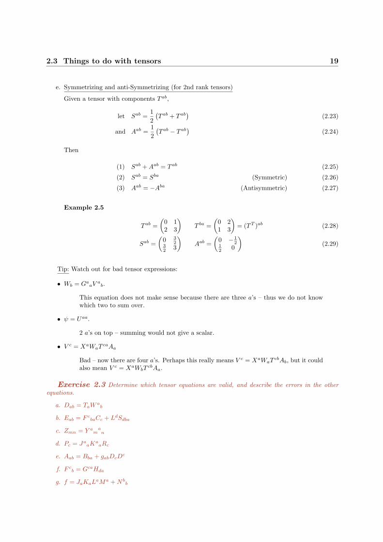
e. Symmetrizing and anti-Symmetrizing (for 2nd rank tensors)
Given a tensor with components T ab,
let Sab =12(T ab + T ab
)(2.23)
and Aab =12(T ab − T ab
)(2.24)
Then
(1) Sab +Aab = T ab (2.25)
(2) Sab = Sba (Symmetric) (2.26)
(3) Aab = −Aba (Antisymmetric) (2.27)
Example 2.5
T ab =(
0 12 3
)T ba =
(0 21 3
)= (TT )ab (2.28)
Sab =(
0 32
32 3
)Aab =
(0 − 1
212 0
)(2.29)
Tip: Watch out for bad tensor expressions:
• Wb = GaaV
ab.
This equation does not make sense because there are three a’s – thus we do not knowwhich two to sum over.
• ψ = Uaa.
2 a’s on top – summing would not give a scalar.
• V c = XaWaTcaAa
Bad – now there are four a’s. Perhaps this really means V c = XaWaTcbAb, but it could
also mean V c = XaWbTcbAa.
Exercise 2.3 Determine which tensor equations are valid, and describe the errors in the otherequations.
a. Dab = TaWa
b
b. Eab = F cbaCc + LdSdba
c. Zmn = Y am
an
d. Pc = JaaK
aaRc
e. Aab = Bba + gabDcDc
f. F cb = GcaHda
g. f = JaKaLaMa +N b
b
20 Tensors and Metrics
Exercise 2.4 Let space be two dimensional, with coordinates (X1,X2). Suppose tensors withcomponents V a, Wa, P ab, Qab, and Ma
b are measured to have the values
V 1 = 2, V 2 = 3; (2.30)W1 = 4, W2 = 5; (2.31)
P ab =(
2 −13 6
)ab
; Qab =(
0 24 7
)ab
; Mab =
(4 32 1
)ab
. (2.32)
Calculate the following tensors:
α = V aWa; (2.33)T b = P abWa; (2.34)F a
c = P abQbc; (2.35)Gab = M c
bQca. (2.36)
Theorem. Let Sab be a symmetric tensor, and Aab an anti-symmetric tensor. Then their doublecontraction vanishes:
AabSab = 0. (2.37)
Proof. To evaluate the double contraction of Aab and Sab, note that we can exchange the dummylabels a and b. Thus
µ ≡ AabSab = AbaS
ba. (2.38)
Now use the symmetry and anti-symmetry of Sab and Aab:
µ = AbaSba = (−Aab)(+Sab) = −µ. (2.39)
This can only be true if the double contraction µ ≡ AabSab is zero.
2.4 The Levi–Civita Tensor
The Levi–Civita tensor is completely antisymmetric. It is actually a tensor density (see section ??).In 2-dimensions:
εab =(
0 1−1 0
)In 3-dimensions:
εab1 =
0 0 00 0 10 −1 0
, (2.40)
εab2 =
0 0 −10 0 01 0 0
, (2.41)
εab3 =
0 1 0−1 0 00 0 0
. (2.42)
Note that all these matrices are anti-symmetric.In general, in N -dimensions:
εab...N =
0 if any 2 of a, b, c, . . . , N are equal1 if (a, b, c, . . . , N) is an even permutation−1 if (a, b, c, . . . , N) is an odd permutation

2.5 3-Vector Identities 21
2.4.1 Odd / Even Permutations
A permutation is an re-ordering. e.g. (4, 2, 1, 3) is a permutation of (1, 2, 3, 4). For N = 3, there are 6permutations:
(1, 2, 3) (1, 3, 2)(2, 3, 1) (2, 1, 3)(3, 1, 2) (3, 2, 1)
We can get from the start (1, 2, 3) to any other permutation by swapping pairs of numbers.Thus swapping 1,2 sends (1,2,3) → (2,1,3), swapping 1,3 sends (2,1,3) → (2,3,1), etc.Similarly, all permutations on N objects can be reached from the identity (1, 2, . . . , N) by a sequence
of swaps. Sometimes two different sequences of swaps will result in the same permutation. But when thishappens both sequences will consist of an even number of swaps, or an odd number of swaps.
Definition 2.5 Even and Odd Permutations Starting from (1, 2, . . . , N), an even number ofswaps results in an even permutation; an odd number of swaps results in an odd permutation.
Example 2.6 N = 4:ε1234 = 1ε1243 = −1ε2143 = 1
(2.43)
2.5 3-Vector Identities
a.−→A ·
−→B = AiBi . (2.44)
b.∇f = ∂if . (2.45)
c. (∇×
−→A)i
= εijk∂jAk (2.46)
Example 2.7 Verify equation (2.46) for the y-component of the curl.Solution The y-component of ∇×
−→A is(
∇×−→A)
y= ε2jk∂jAk (2nd component = y-component)
= ε231∂3A1 + ε213∂1A3
= (1)∂
∂zAx + (−1)
∂
∂xAz
=∂Ax
∂z− ∂Az
∂x.
Example 2.8 Show that−→A ×
−→B = −
−→B ×
−→A. (2.47)
Solution Translate to (−→A ×
−→B)i
= εijkAjBk.

22 Tensors and Metrics
but εijk = −εikj
⇒(−→A ×
−→B)i
= −εikjAjBk
= −εikjBkAj
(Aj and Bk are just numbers, so we can reverse their order in a multiplication without affecting theresult).
Now we replace the dummy indices j → k and k → j. They are being summed over, so it does notmatter which one is called which:
⇒(−→A ×
−→B)i
= −εijkBjAk
= −(−→B ×
−→A)i
∴−→A ×
−→B = −
−→B ×
−→A .
Example 2.9 Show that
∇×∇f = 0. (2.48)
Solution Translate to
(∇×∇f)i = εijk∂j∂kf
= εijk∂k∂jf (partial derivatives commute)
= −εikj∂k∂jf
relabel j ↔ k
⇒ (∇×∇f)i = −εijk∂j∂kf
⇒ (∇×∇f)i = − (∇×∇f)i
⇒ (∇×∇f)i = 0
∴ ∇×∇f = 0
Exercise 2.5 Translate the following 3-vector identities into index notation, and prove them:
A · (B×C) = B · (C×A) = C · (A×B); (2.49)∇ · (fA) = A · ∇f + f∇ ·A; (2.50)
∇ · (A×B) = B · ∇ ×A−A · ∇ ×B. (2.51)
2.6 Metrics 23
2.6 Metrics
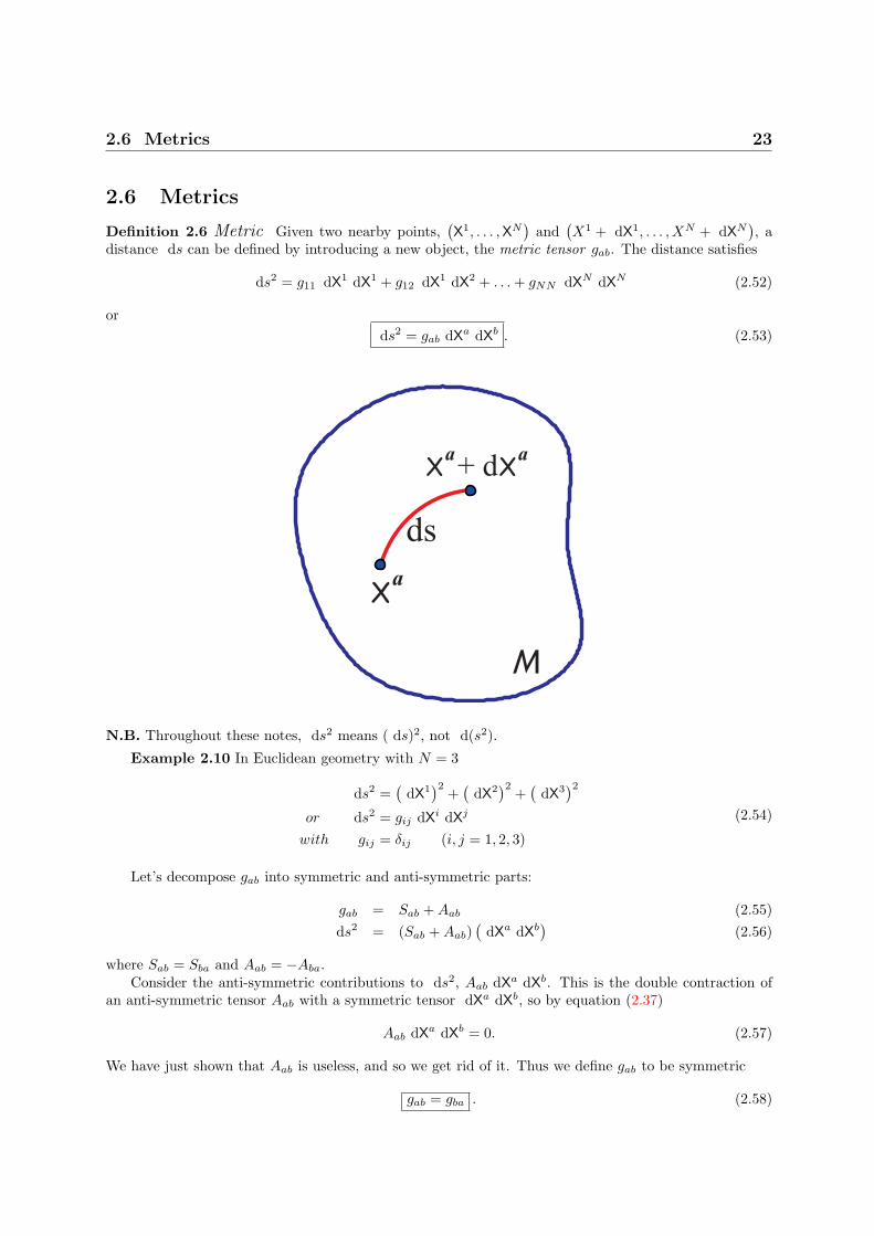
Definition 2.6 Metric Given two nearby points,(X1, . . . ,XN
)and
(X1 + dX1, . . . , XN + dXN
), a
distance ds can be defined by introducing a new object, the metric tensor gab. The distance satisfies
ds2 = g11 dX1 dX1 + g12 dX1 dX2 + . . .+ gNN dXN dXN (2.52)
ords2 = gab dXa dXb . (2.53)
N.B. Throughout these notes, ds2 means ( ds)2, not d(s2).
Example 2.10 In Euclidean geometry with N = 3
ds2 =(
dX1)2
+(
dX2)2
+(
dX3)2
or ds2 = gij dXi dXj
with gij = δij (i, j = 1, 2, 3)
(2.54)
Let’s decompose gab into symmetric and anti-symmetric parts:
gab = Sab +Aab (2.55)ds2 = (Sab +Aab)
(dXa dXb
)(2.56)
where Sab = Sba and Aab = −Aba.Consider the anti-symmetric contributions to ds2, Aab dXa dXb. This is the double contraction of
an anti-symmetric tensor Aab with a symmetric tensor dXa dXb, so by equation (2.37)
Aab dXa dXb = 0. (2.57)
We have just shown that Aab is useless, and so we get rid of it. Thus we define gab to be symmetric
gab = gba . (2.58)

24 Tensors and Metrics
How many components does gab have? If the manifold is N dimensional, then an arbitrary tensorof rank r has Nr components. But since the metric is symmetric, not all these components will beindependent.
gab =
g11 g12 . . . g1N
g21 g22 . . . g2N
......
gN1 gN2 . . . gNN
︸ ︷︷ ︸
N2 components
. (2.59)
By symmetry (gab = gba),
⇒ gab =
g11 g12 g13 . . . g1N
g12 g22 g23 . . . g2N
g13 g23 g33 . . . g3N
......
g1N g2N g3N . . . gNN
= gba (2.60)
so there are N(N+1)2 independent components.
2.7 Euclidean Metrics
E2 – Euclidean PlaneCartesian: By the Pythagorean theorem,
ds2 =(
dC1)2
+(
dC2)2
= dx2 + dy2 (2.61)
= gC11 dx2 + g
C12 dx dy + gC21 dy dx+ g
C22 dy2. (2.62)
So gC11 = g
C22 = 1 while gC12 = g
C21 = 0, or
gCab =
(1 00 1
).
Polars:Two methods to find the metric:

2.7 Euclidean Metrics 25
Method 1: Draw pictures:
a = 2(r + dr) sin(
dφ2
)(2.63)
= 2(r + dr)(
dφ2
)(+O( dφ)3) (2.64)
= r dφ (+O( dr dφ)). (2.65)
Thusds2 = dr2 + r2 dφ2 (2.66)
or, in terms of the metric tensor ds2 = gab dPa dPb,
gP ab =
(1 00 r2
). (2.67)
Method 2:We know that
gCab =
(1 00 1
)∴ g
P ab =∂Cc
∂Pa
∂Cd
∂Pb
(1 00 1
)cd
.
(Cartesians on top (c,d), polars on bottom (a,b)).
2.7.1 E3 Euclidean 3-space
Cartesian:
gCab =
1 0 00 1 00 0 1
. (2.68)
Spherical:
• If we just move in r:
ds2r = dr2 (2.69)
• If we just move in θ, we move on a radiusr:
ds2θ = r2 dθ2 (2.70)
• If we just move in φ, we move on a con-stant radius r sin θ:
ds2φ = r2 sin2 θ dφ (2.71)
26 Tensors and Metrics
Thus
ds2 = dr2 + r2 dθ2 + r2 sin2 θ dφ2 (2.72)
gP ab =
1 0 00 r2 00 0 r2 sin2 θ
. (2.73)
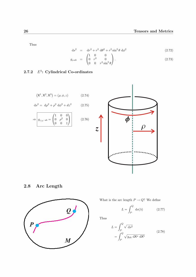
2.7.2 E3: Cylindrical Co-ordinates
(X1,X2,X3
)= (ρ, φ, z) (2.74)
ds2 = dρ2 + ρ2 dφ2 + dz2 (2.75)
⇒ gCyl ab =
1 0 00 ρ2 00 0 1
(2.76)
2.8 Arc Length
What is the arc length P → Q? We define
L =∫ Q
P
ds(λ) (2.77)
Thus
L =∫ Q
P
√ds2
=∫ Q
P
√gab dXa dXb
(2.78)
2.9 Scalar Product and Magnitude for Vectors 27
Example 2.11 E2 with Cartesian coordinates. Here
L =∫ Q
P
√dx2 + dy2. (2.79)
We can divide by√
dλ2 and multiply by dλ to make
L =∫ Q
P
√(dxdλ
)2
+(
dydλ
)2
dλ. (2.80)
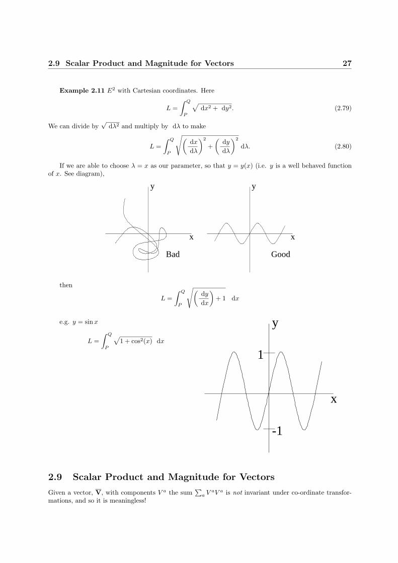
If we are able to choose λ = x as our parameter, so that y = y(x) (i.e. y is a well behaved functionof x. See diagram),
������������������������������
y
x
Bad
������������������������������
y
x
Good
then
L =∫ Q
P
√(dydx
)+ 1 dx
e.g. y = sinx
L =∫ Q
P
√1 + cos2(x) dx
����������������������������
����������������������������
����������������������������
y
x
1
-1
2.9 Scalar Product and Magnitude for Vectors
Given a vector, V, with components V a the sum∑
a VaV a is not invariant under co-ordinate transfor-
mations, and so it is meaningless!

28 Tensors and Metrics
But, if we have a metric, we can define
V ·V = gabVaV b This is invariant! (2.81)
The magnitude of V is
∣∣V∣∣ =√V ·V (2.82)
Similarly, with two vectors V,WV ·W = gabV
aW b (2.83)
For two forms A,BA ·B = gabAaBb (2.84)
where gab is the inverse of the metric tensor, in the sense that
gabgbc = δac. (2.85)
Also ∣∣A∣∣ =√A ·A. (2.86)
2.10 Raising and Lowering Operators
Note that V ·W = gabVaW b is a scalar. We can write this as
V ·W = (gabVa)W b (2.87)
Then gabVa is ‘dual’ to the set of vectors – It takes a vector, W, and returns a scalar number. Therefore,
given a vector V, we can define a form V where
Vb = gabVa. (2.88)
Similarly
V ·W = V a(gabW
b)
(2.89)
⇒Wa = gabWb (2.90)
⇒ V ·W = V aWb (2.91)= VbW
a (2.92)
By contraction with the metric, we can ‘raise’ or ‘lower’ the index.Exercise 2.6 Suppose that Aab is anti-symmetric. Let Aab = gacgbdA
cd where gac is the (sym-metric) metric tensor. Show that Aab is antisymmetric as well.
Exercise 2.7 Let
T ab =(
2 35 7
). (2.93)
Find its symmetric and antisymmetric parts Aab and Sab. Next, let the metric be
gab =(
1 22 1
). (2.94)
Find Aab. Show explicitly thatAabS
ab = 0. (2.95)

2.11 Signature of the Metric 29
2.11 Signature of the Metric
One can show, using linear algebra, that any metric, gab, can be diagonalized by transforming to a suitableco-ordinate system.
e.g. If in coordinates X, the metric is
gab =(−3 −5−5 62
)Then there exists coordinates X′ where
g′ab =(
1 00 −1
)In general, we can make the values on the diagonal 1 or -1 by transforming to suitable co-ordinates
• Find eigenvectors and eigenvalues of gab
• Transform to co-ordinates along the eigenvectors (diagonalize metric)
• divide each eigenvector by it’s eigenvalue (all go to 1,-1)
There may be a few ways of doing this. However, it can be shown that the sum of the diagonalelements will always be the same. This is called the signature of the metric.
Example: E3 with Cartesian coordinates
gab =
1 0 00 1 00 0 1
(2.96)
Signature = 3.
Example: Minkowski Metric
gab = ηab =
1 0 0 00 −1 0 00 0 −1 00 0 0 −1
(2.97)
Signature = -2.
2.12 Riemannian and Pseudo-Riemannian metrics
Is the magnitude of a vector always positive?Definition 2.7 Riemannian metric For a Riemannian metric, any vector V 6= 0 satisfies
||V||2 = V ·V > 0. (2.98)
A metric which is not Riemannian is called Pseudo-Riemannian.
• Signature = N metrics are Riemannian.To see this note that we can calculate V ·V (at some point P ) in any coordinate system, includingthe system with only ±1 diagonal elements for the metric. Then
V ·V = gabVaV b = ±(V 1)2 ± (V 2)2 ± ...± (V N )2. (2.99)
If signature = N then there will be only pluses, and the sum will be positive.

30 Tensors and Metrics
• Signature < N metrics are pseudo-Riemannian.On the other hand, if the signature is less than N , then there will be some minuses in the sum.Say for example that V ·V = (V 1)2 + (V 2)2 + · · · + (V n−1)2 − (V N )2. Then we could choose avector V whose only non-zero element is V N . This would make V ·V < 0.
Euclidean metrics are Riemannian, while the Minkowski metric is pseudo-Riemannian.
2.13 Map Projections
The Earth, radius r = R = constant, has the metric line element (in spherical coordinates S = (θ, φ))
ds2 = R2(
dθ2 + sin2 θ dφ2), (2.100)
with 0 ≤ θ ≤ π, −π ≤ φ ≤ π.
⇒ gSab = R2
(1 00 sin2 θ
)(2.101)
2.13.1 Cylindrical Map
Globe
PaperProject outonto paper
y
x
0 ππx
y
We wish to project the Earth onto a piece of paper of width w and height h. The co-ordinates onthe map will be M = (x, y) with
x =w
2πφ (2.102)
y =h
2cos θ (2.103)
yθ
θRcos
Let us call the metric for the map projection gM ab . Using this metric we can calculate the arclength
of any path drawn on the map (from Buenos Aires to Glasgow for example). The calculation will givethe distance along the corresponding path on the Earth’s surface.
2.13 Map Projections 31
Problem: find the metric gM ab .
Method 1: Use the transformation law for tensors:
gM ab =
∂Mc
∂Sa
∂Md
∂Sbg
Scd . (2.104)
Method 2: Directly transform the metric line element: first,
ds2 = R2(
dθ2 + sin2 θ dφ2)
(2.105)
dφ =2πw
dx (2.106)
⇒ ds2 = R2
(dθ2 +
4π2
w2sin2 θ dx2
). (2.107)
Next, from the formula for y,
dy = −h2
sin θ dθ (2.108)
⇒ dθ2 =4h2
dy2
sin2 θ. (2.109)
Also,
sin2 θ = 1−(
2yh
)2
(2.110)
⇒ dθ2 =4 dy2
h2 − 4y2. (2.111)
Thus
ds2 = R2
(4π2
w2
h2 − 4y2
h2dx2 +
4h2 − 4y2
dy2
). (2.112)
Changing the aspect ratio w/h will stretch or compress the map in the vertical direction. We should choosethis ratio to give the least distortion. Note that at y = 0 (the equator) the y dependence disappears. Themetric will be symmetric in x and y at the equator if w = πh. In this case, the line element and metricare
ds2 = 4R2
(h2 − 4y2
h4dx2 +
1h2 − 4y2
dy2
). (2.113)
gab = 4R2
(h2−4y2
h4 00 1
h2−4y2
). (2.114)
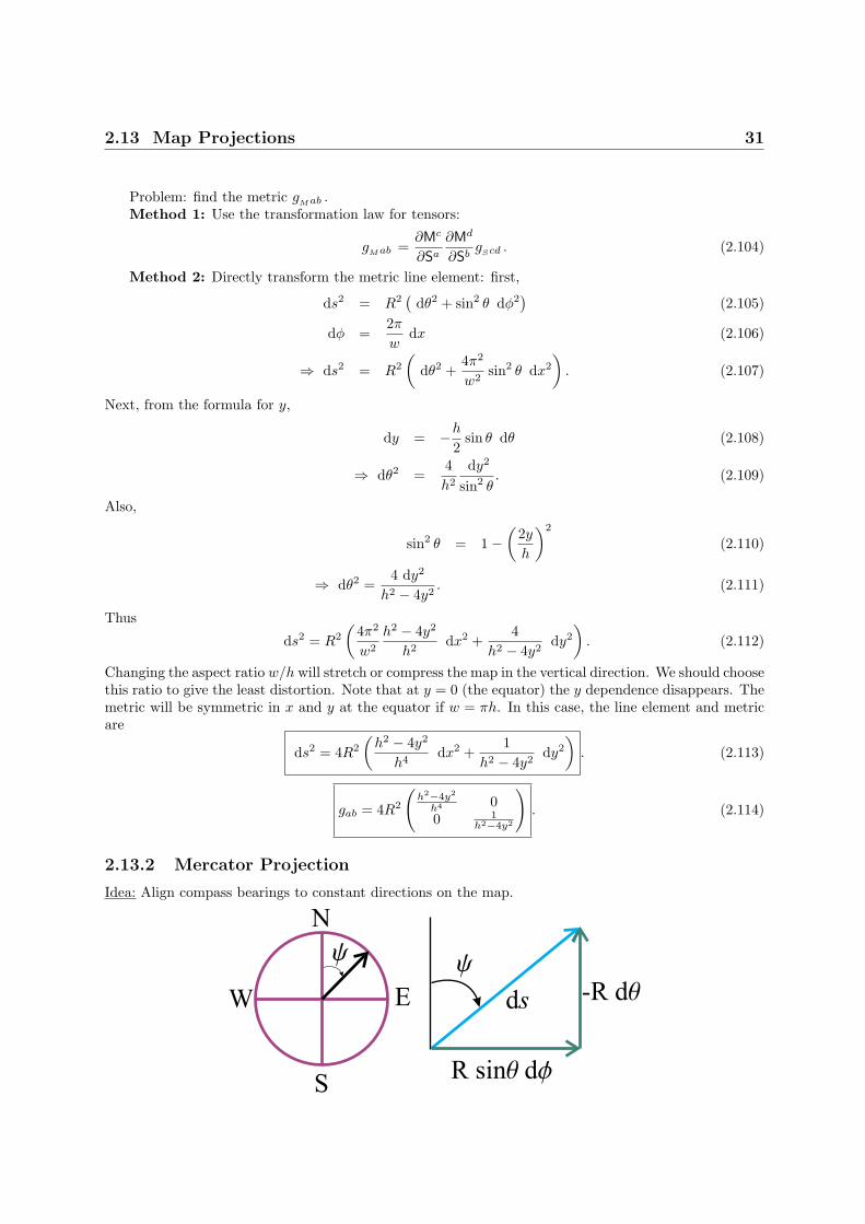
2.13.2 Mercator Projection
Idea: Align compass bearings to constant directions on the map.

32 Tensors and Metrics
ds2 = a2 + b2 (2.115)a = R sin θ dθ (2.116)b = −R dθ (2.117)
⇒ ds2 = R2(
dθ2 + sin2 θ dφ2)
(2.118)
Again, let x = w2π φ.
Choose y so that the slope of dydx of a curve is a constant for constant ψ:
cotψ =−R dθ
R sin θ dφ= − 1
sin θdθdφ. (2.119)
On the map, however,
cotψ =dydx
(2.120)
= − 1sin θ
dθdφ
= − w
2π1
sin θdθdx
(2.121)
⇒ dydθ
= − w
2π1
sin θ(2.122)
After integration,
y =∫ y
0
dy′ = − w
2π
∫ 0
θ
dθsin θ
(2.123)
∴ y =w
2πlog[cot
θ
2
](2.124)
We can now find gM ab . First, we derive a simple identity: let
y ≡ 2πwy = log
[cot
θ
2
].
Thensin θ =
1cosh y
= sech y.
Proof:
sech y =2
ey + e−y
=2
cot θ/2 + tan θ/2
=2
cot θ/2(1 + tan2 θ/2
)=
2cot θ/2 (sec2 θ/2)
= 2 cos θ/2 sin θ/2.
Now
ds2 = R2(
dθ2 + sin2 θ dφ2)
=(
2πw
)2
R2((− sin θ dy)2 + sin2 θ dx2
)
2.13 Map Projections 33
Thus we have found the Mercator line element:
ds2 =(
2πRw
)2
sech 2y(
dx2 + dy2), (2.125)
and the Mercator metric:
gM ab =
(2πRw
)2
sech 2y
(1 00 1
). (2.126)
Exercise 2.8 London has latitude 51◦ and longitude 0◦. Suppose you travel on the surface of theearth, following a geodesic (great circle) which leaves London in the direction due East. Where will youfirst hit the equator? (This problem can be done without any equations!)


