Cable Stay Fatigue Analysis for the Fred Hartman Bridge by John C. Eggers, B.S.C.E. Thesis Presented to the Faculty of the Graduate School of The University of Texas at Austin in Partial Fulfillment of the Requirements for the Degree of Master of Science in Engineering The University of Texas at Austin August 2003
Transcript
Cable Stay Fatigue Analysis for the
Fred Hartman Bridge
by
John C. Eggers, B.S.C.E.
Thesis
Presented to the Faculty of the Graduate School of
The University of Texas at Austin
in Partial Fulfillment
of the Requirements
for the Degree of
Master of Science in Engineering
The University of Texas at Austin
August 2003
Cable Stay Fatigue Analysis for the
Fred Hartman Bridge
Approved by Supervising Committee:
Dr. Sharon Wood, Supervisor
Dr. Karl Frank, Supervisor
Dedication
I would like to dedicate this thesis to my parents, my father and mother in-
law, and my beautiful, patient, and loving wife, Jennifer.
iv
Acknowledgements
I would like to thank the Texas Department of Transportation for
sponsoring this project at the Ferguson Structural Engineering Laboratory (FSEL)
at The University of Texas at Austin.
I would like to also give my appreciation to the many professors that
assisted in my research. Specifically I would like to thank Dr. Sharon Wood and
Dr. Karl Frank for their advice and dedication to this project.
A large amount of manual labor was required for this project. I would like
to thank Tammer Botros and Meg Warpinski for their companionship, labor, and
ideas throughout the project. The lab technicians who include Blake Stassney,
Mike Bell, and Dennis Fillip provided invaluable assistance throughout the
project. Their experience and knowledge of the laboratory environment provide
an enormous amount of assistance to every research project at FSEL.
I would also like to thank my fellow graduate students for making life at
FSEL and The University of Texas enjoyable.
May 2003
v
Abstract
Cable Stay Fatigue Analysis for the
Fred Hartman Bridge
John C. Eggers, M.S.E.
The University of Texas at Austin, 2003
Supervisors: Sharon Wood, Karl Frank
Topics covered in this thesis include analysis and testing of single-strand specimens under tension and static bending loads, including the development of closed-form solutions to estimate the bending moment in a single strand under tension and bending. It also includes tensile fatigue characterization of strand. In addition, there is the characterization and analysis of vibration data from the Fred Hartman Bridge, including integration of acceleration data to attain displacement records and rainflow cycle counting analyses.
VITA ...................................................................................................................108
ix
List of Tables
Table 1.1Full-Sized Specimen Test Summary........................................................6 Table 2.1 Difference between FEM and Measured Response ..............................11 Table 2.2 Measured Stiffness of Various Specimens ............................................22 Table 2.3 Stiffnesses of Closed-form Solution and Measured Response..............29 Table 2.4 Estimated Moments in Strand 3, Test 2 ................................................32 Table 3.1 Single-strand Fatigue Test Results........................................................41 Table 3.2 PTI Specification Strand Fatigue Requirements ...................................43 Table 4.1 Cable Identification and Lengths ..........................................................47 Table 4.2 Maximum Displacements at Accelerometer Locations (in.) .................54 Table 4.3 Measured Natural Frequency of Stay-Cables........................................55 Table 4.4 Primary Vibration Mode of Cables .......................................................56 Table 4.5 Rainflow Results for File No. 199710010.............................................58 Table 4.6 Rainflow Results for File No. 199710010.............................................60 Table 4.7 Equivalent Displacements for each Cable During ................................61 Table 4.8 Overall Equivalent Displacements and .................................................62 Table 4.9 Total Number of Wind-Rain Cycles for Each Cable ............................63 Table 4.10 Summary of the Number of Cycles to the First Wire Break in...........63 Table 4.11 Summary of Estimated Fatigue for .....................................................64 Table B.1 Single Strand Test Summary................................................................84
x
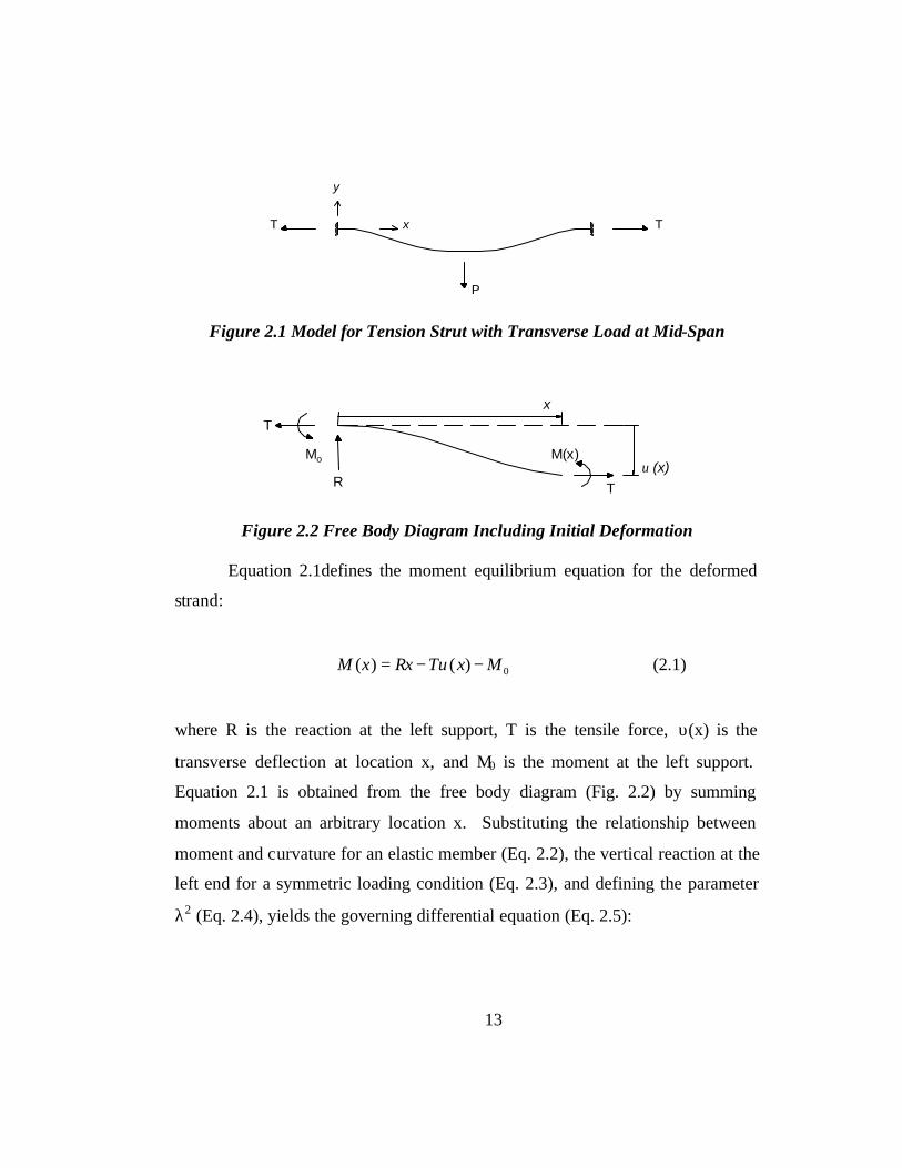
List of Figures
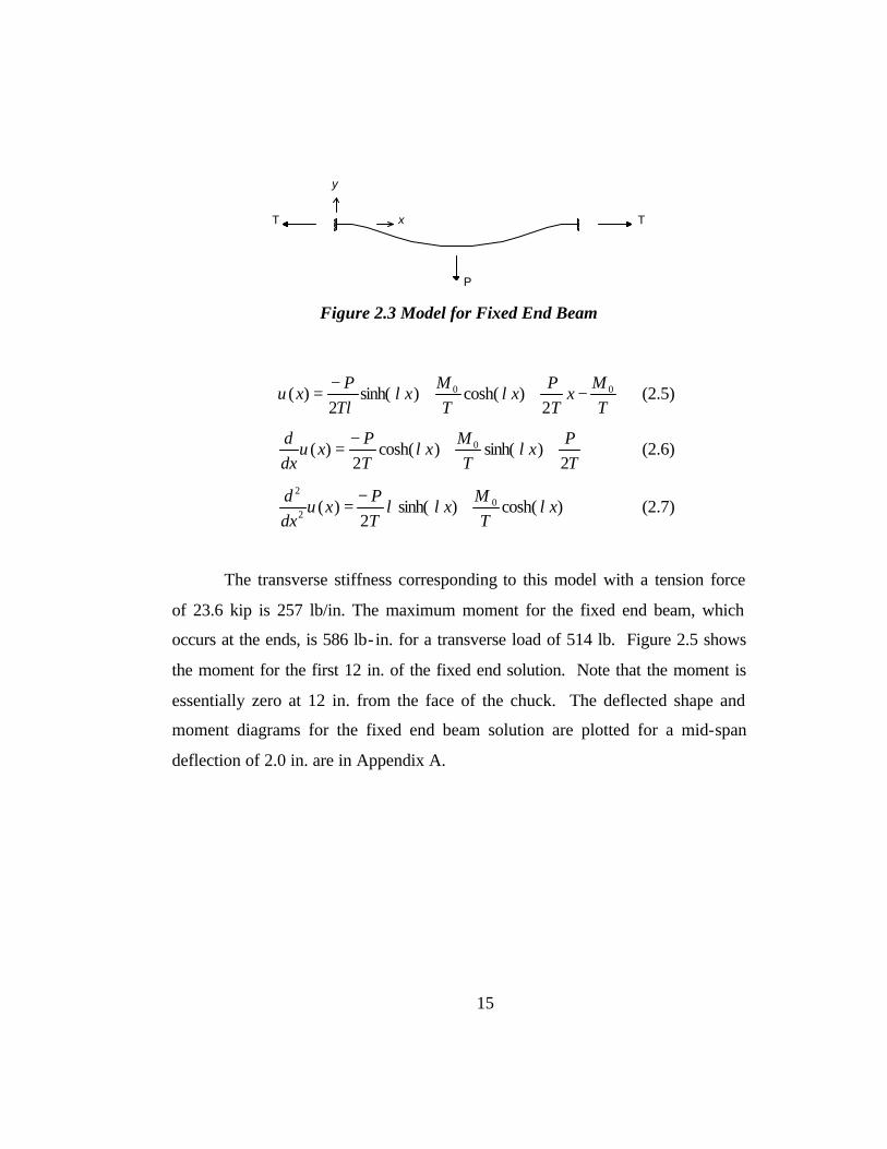
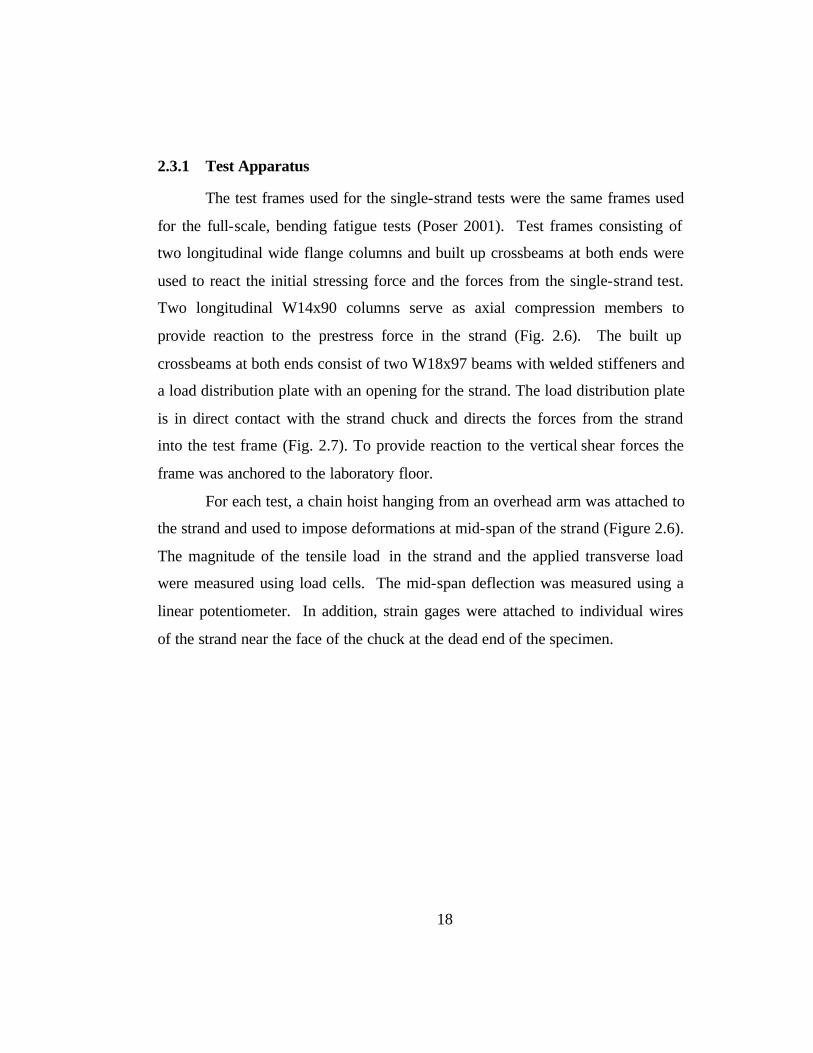
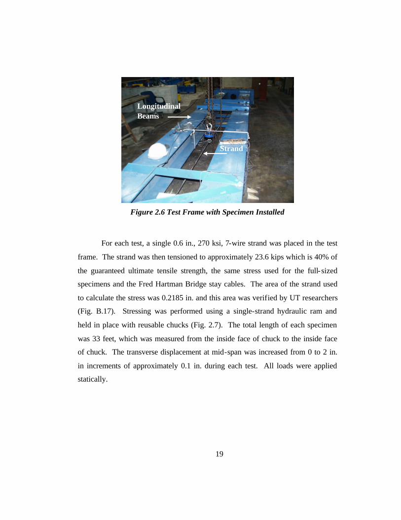
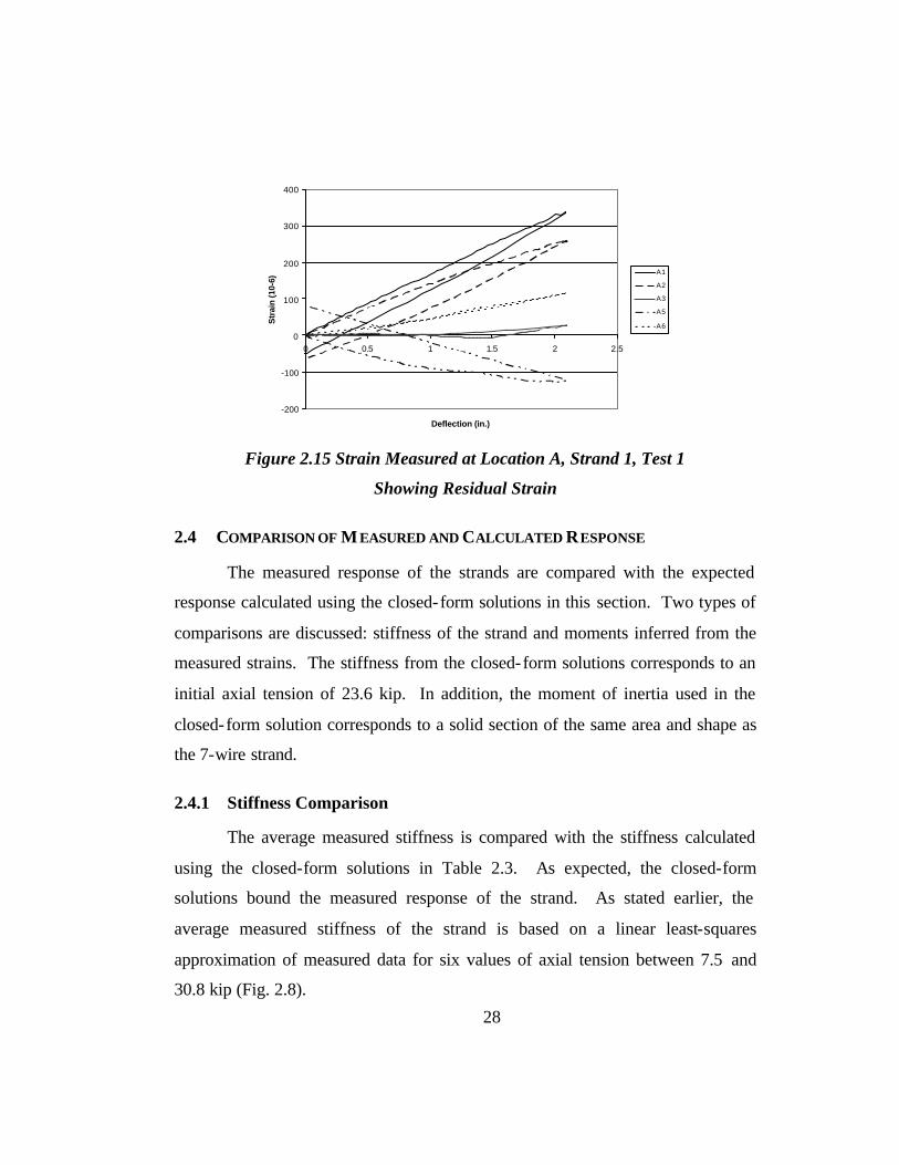
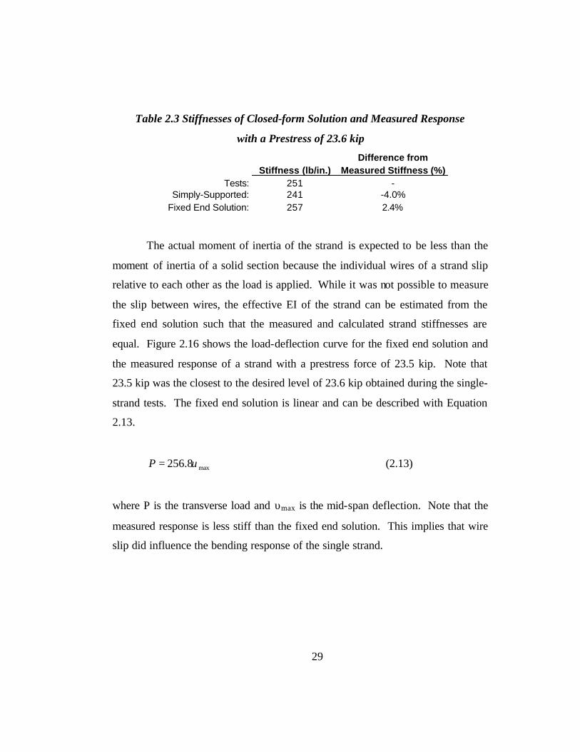
Figure 1.1 Fred Hartman Bridge .............................................................................1 Figure 1.2 Two Independent Deck of the Fred Hartman Bridge .............................2 Figure 2.1 Model for Tension Strut with Transverse Load at Mid-Span ..............13 Figure 2.2 Free Body Diagram Including Initial Deformation..............................13 Figure 2.3 Model for Fixed End Beam..................................................................15 Figure 2.4 Moment Diagram for Fixed end Beam................................................16 Figure 2.5 Model for Simply-Supported Beam.....................................................17 Figure 2.6 Test Frame with Specimen Installed ....................................................19 Figure 2.7 Stressing of Single-strand ....................................................................20 Figure 2.8 Stiffness vs. Prestress Force .................................................................21 Figure 2.9 Stiffness vs. Deflection of Single-strand for a .....................................23 Figure 2.10 Tensile Load vs. Deflection of Single-strand for a ............................24 Figure 2.11 Location of Strain Gages for Strand 3, ..............................................24 Figure 2.12 Strain Measured at Location A, Strand 3, Test 2 ...............................25 Figure 2.13 Approximate Location of Strain Gages at Location A ......................26 Figure 2.14 Strain Measured at Location B, Strand 3, Test 2 ...............................27 Figure 2.15 Strain Measured at Location A, Strand 1, Test 1 ...............................28 Figure 2.16 Comparison of Load-Deflection Curves for Test 2 of Strand 3 and the
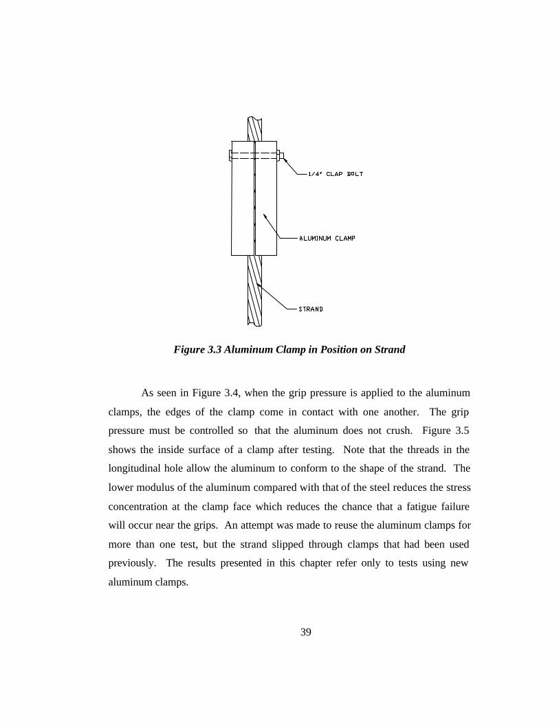
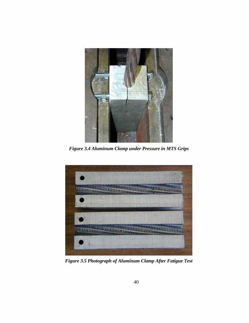
Fixed End Solution........................................................................................30 Figure 2.17 Cross-section Stress Diagram for a Single-Strand in Bending Figure 3.1 Schematic of Test Set-up .....................................................................36 Figure 3.2 Schematic of Aluminum Clamp...........................................................38 Figure 3.3 Aluminum Clamp in Position on Strand ..............................................39 Figure 3.4 Aluminum Clamp under Pressure in MTS Grips .................................40 Figure 3.5 Photograph of Aluminum Clamp After Fatigue Test...........................40 Figure 3.6 Tensile Fatigue Test Results ................................................................44 Figure 4.1 Schematic of South Tower Profile View .............................................48 Figure 4.2 Schematic of South Tower Plan View .................................................48 Figure 4.3 Acceleration-time Record for Cable AS9 ............................................49 Figure 4.4 Velocity Record for Cable AS9 without Filtering or Smoothing ........51 Figure 4.5 Velocity Record for Cable AS9 with Filtering and Smoothing ...........51 Figure 4.6 Lissajous Diagram of Cable AS9 for 1 Second of Time......................53 Figure 4.7 Accelerometer Locations vs. Possible Mode Shapes ...........................56 Figure A.1 Fixed-Fixed Beam Free Body Diagram..............................................72 Figure A.2 Fixed-Fixed Beam Deflection Diagram..............................................74 Figure A.3 Fixed-Fixed Beam Moment Diagram .................................................75 Figure A.4 Fixed-Fixed Beam Moment Diagram for T ˜ 0 kip ............................76 Figure A.5 Simply-Supported Beam Free Body Diagram ....................................77 Figure A.6 Simply-Supported Deflected Shape ....................................................80
xi
Figure A.7 Simply-Supported Beam Moment Diagram........................................81 Figure A.8 Simply-supported Beam Moment Diagram for T ˜ 0 kip ...................82 Figure B.1 Strand 1, Test 1 at a Prestress of 7.5 kip .............................................85 Figure B.2 Strand 1, Test 1 at a Prestress of 7.5 kip .............................................85 Figure B.3 Strand 1, Test 2 at a Prestress of 21.4 kip ...........................................86 Figure B.4 Strand 1, Test 2 at a Prestress of 21.4 kip ...........................................86 Figure B.5 Strand 2, Test 1 at a Prestress of 14.5 kip ...........................................87 Figure B.6 Strand 2, Test 1 at a Prestress of 14.5 kip ...........................................87 Figure B.7 Strand 2, Test 2 at a Prestress of 20.9 kip ...........................................88 Figure B.8 Strand 2, Test 2 at a Prestress of 20.9 kip ...........................................88 Figure B.9 Strand 2, Test 3at a Prestress of 23.3 kip ............................................89 Figure B.10 Strand 2, Test 3 at a Prestress of 23.3 kip .........................................89 Figure B.11 Strand 3, Test 1 at a Prestress of 21.9 kip .........................................90 Figure B.12 Strand 3, Test 1 at a Prestress of 21.9 kip .........................................90 Figure B.13 Strand 3, Test 2 at a Prestress of 23.5 kip .........................................91 Figure B.14 Strand 3, Test 2 at a Prestress of 23.5 kip .........................................91 Figure B.15 Strand 3, Test 3 at a Prestress of 30.8 kip .........................................92 Figure B.16 Strand 3, Test 3 at a Prestress of 30.8 kip .........................................92 Figure B.17 Strand Specification Sheet.................................................................93 Figure B.17 Strand Size Verification ....................................................................94
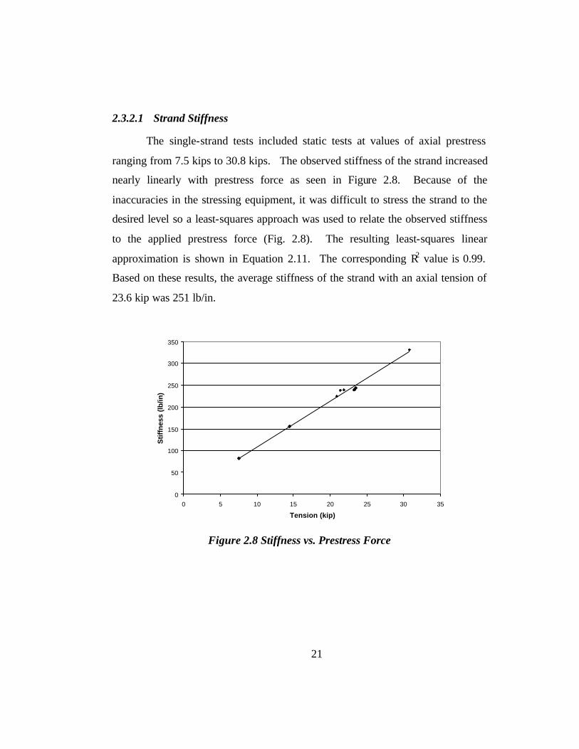
1
CHAPTER 1
Introduction
1.1 FRED HARTMAN BRIDGE
Construction was completed on the Fred Hartman Bridge (Fig. 1.1) on
September 27, 1995. The bridge crosses the Houston shipping channel between
Baytown and La Port, Texas and was constructed to replace the Baytown-La
Porte Tunnel.
Figure 1.1 Fred Hartman Bridge
2
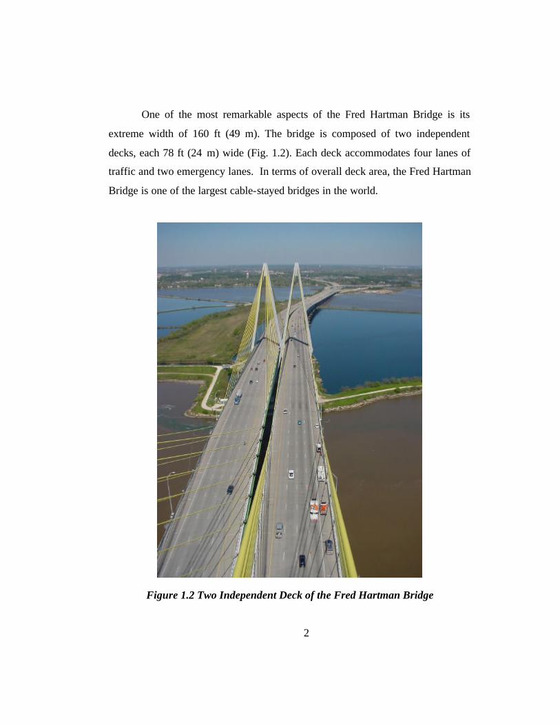
One of the most remarkable aspects of the Fred Hartman Bridge is its
extreme width of 160 ft (49 m). The bridge is composed of two independent
decks, each 78 ft (24 m) wide (Fig. 1.2). Each deck accommodates four lanes of
traffic and two emergency lanes. In terms of overall deck area, the Fred Hartman
Bridge is one of the largest cable-stayed bridges in the world.
Figure 1.2 Two Independent Deck of the Fred Hartman Bridge
3
The following is a summary of information about the Fred Hartman
Bridge (National Web Window, 2001):
o Total length: 2,475 ft
o Main span: 1250 ft
o Building time: 9 years from 1986 until 1995
o Capacity: 200,000 vehicles per day (Baytown tunnel: 25,000 per day)
o Cost: 100 million US Dollars
o Double diamond towers - 436 ft (133 m) tall
o Fan-type arrangement of the stay cables
o 192 cables, the longest stretching 650 ft (198 m)
o Over 618 miles of cable strand
o More than 40,000,000 pounds (18,145 t) of steel
o More than 3,000,000 ft3 (48,951 m3) of concrete
1.2 CABLE VIBRATION PROBLEMS
Since construction, wind-rain induced vibrations have been observed in
the stay-cables of the Fred Hartman Bridge. Wind-rain induced vibrations are
produced when rainwater forms rivulets under the influence of the airflow around
the cable, which then changes the aerodynamic cross section of the stay cable in
such a way that it is susceptible to vibrations (Poser 2002). The Texas Department
of Transportation (TXDoT) has since initiated a research project to:
o Design repair solutions for existing damage caused by the vibrations
4
o Design structural and aerodynamic solutions to eliminate or control
cable vibrations
o Characterize the vibrations so the mechanics are better understood and
efficient damping can be designed to control the vibrations
o Characterize the fatigue behavior of the cables and estimate the
amount of fatigue damage caused by the wind-rain induced vibrations
Engineers from Whitlock, Dalrymple, Poston, and Associates (WDP),
Johns Hopkins University (JHU), Texas Tech University (TTU), and the
University of Texas at Austin (UT) form the team developed by TxDOT to
investigate the wind-rain induced vibration phenomenon observed on the Fred
Hartman Bridge.
WDP developed designs to repair the existing damage, and reduce the
cable vibrations. Solutions that have been installed include the following:
o stiffened guide pipe connections to withstand the large forces induced
by cable vibrations
o installation of cable restrainers which allow cables that are excited by
wind-rain induced vibration to be restrained by adjacent cables to
reduce the effective length of the cables
o installation of dampers which reduce the amplitude of the vibrations
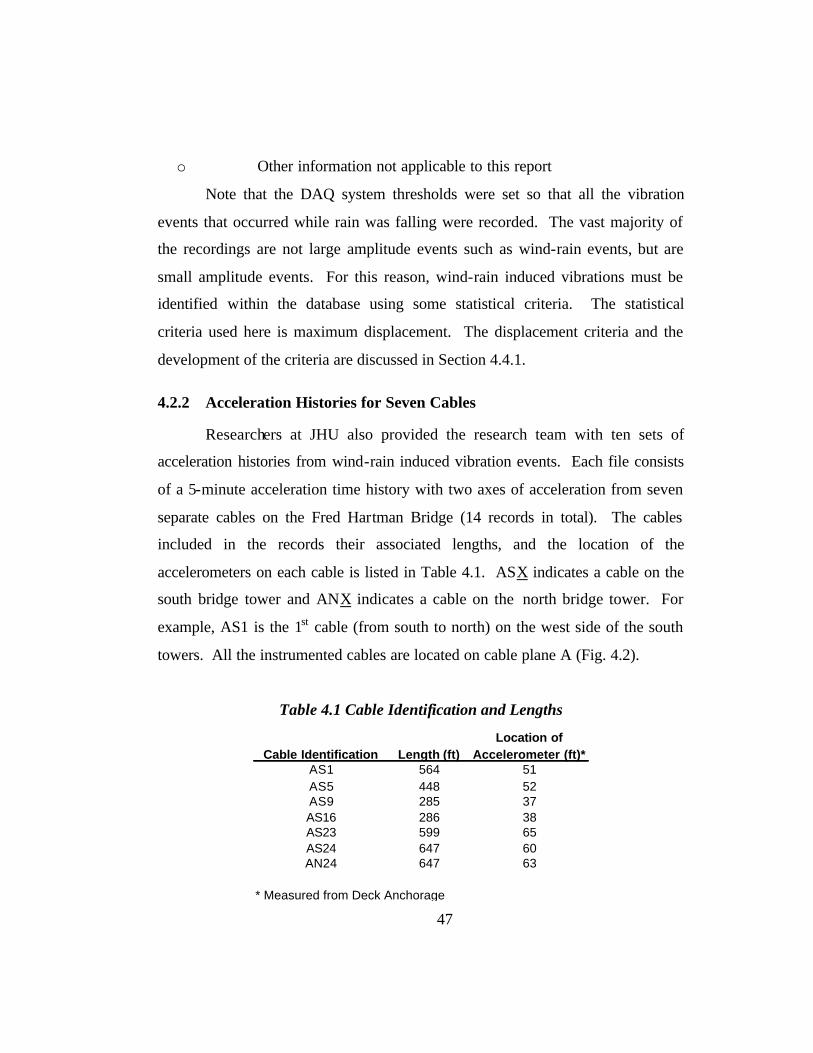
Researchers from Johns Hopkins University instrumented several cables
on the Fred Hartman Bridge in October of 1997 to identify the vibrational
characteristics. The vibrational characteristics are essential for understanding the
mechanics of the wind-rain vibrations and to design efficient damping solutions.
Researchers from JHU have developed a statistical database containing cable
5
vibration characteristics and weather data for each recorded vibration event since
October 1997.
Researchers from Texas Tech University developed an aerodynamic
damping solution. Their proposed solution consists of a number of rings wrapped
around the cable to prevent the formation of the rainwater rivulets (Sarker 1999).
The research team from the University of Texas (UT) has focused on
characterizing the fatigue behavior of the cables. The research program consists
of three phases:
1. Instrument the stay cables on the Fred Hartman Bridge to
determine the relationship between measured strains and
accelerations dur ing a wind-rain vibration event
2. Assemble and test ten full-size fatigue tests in the laboratory to
determine their fatigue behavior
3. Develop computational models of the full-sized test specimens
and the Fred Hartman stay cables. Use the models to relate the
observed fatigue behavior of the test specimens to cables with
different lengths and diameters on the bridge.
1.3 RESEARCH CONDUCTED AT THE UNIVERSITY OF TEXAS
1.3.1 Field Measurments
As of May 2003, the research team at UT has attempted to measure strains
at various locations on the Fred Hartman Bridge. The exterior polyethylene (PE)
sheathing of the stay cables, the surface of the grout just below the PE sheathing,
and the guide pipes attaching the cables to the deck. The field measurements
were largely unsuccessful. For various reasons, the strain gages either did not
6
adhere correctly, corroded rapidly, or provided limited data (Poser 2001). Future
attempts to gage the cables are not planned.
The accelerations of the stay cables were monitored by the JHU research
team. Although the monitoring system was not completely reliable, these
accelerometers have provided useful data during wind-rain induced vibrations. It
is anticipated that researchers at the University of Texas will be able to correlate
these data to stress with using the computational models.
1.3.2 Full-Scale Bending Fatigue Testing
As of May 2003, five full-size cable stay fatigue tests have been
completed. Each test specimen was constructed similar to the smallest stay cable
on the bridge, and the length of each specimen was approximately 33 ft. For each
test, parameters such as the grout mix design, transverse displacement amplitude,
and other construction variables were varied. An overview of the 5 full-sized
tests is shown in Table 1.1. The 2001 thesis by Poser documents the behavior of
the first two specimens.
Table 1.1Full-Sized Specimen Test Summary
Specimen Displacement Testing Total NumberNo. Amplitude (+/- in.) Frequency (Hz) of Cycles1 1.60 0.9 2,808,3982 1.60 0.7 2,865,1033 1.60 2.2 4,961,5604 1.10 3.0 8,775,2455* 1.60 3.0 5,211,056
* Specimen 5 was ungrouted and there were no wire failures
7
1.3.3 Computational Models
Previously on this project, Dowd (2001) developed a finite element model
(FEM) of the full-scale strand specimen using beam elements and transformed
sections. Comparison of the FEM model and the results of the full-scale test
described above indicated that the FEM model overestimates the cable stiffness
by nearly a factor of 2. Further refinement of the FEM model is needed to
develop a more realistic model of the test specimens.
1.4 TOPICS COVERED IN THIS THESIS
This thesis describes research activities related to three different
components of the UT research project. While this thesis does not discuss the
results of the full-scale tests or the development of the computational models
specifically, it does describe research related to the research at UT. Topics
covered in this thesis include analysis and testing of single-strand specimens
under tension and static bending loads, tensile fatigue characterization of strand
used to construct full-scale specimens 1 through 6, and characterization and
analysis of vibration data from the Fred Hartman Bridge.
1.4.1 Single Strand Bending Tests
Chapter 2 of this thesis describes the testing of three single-strand
specimens under tension and static bending and the development of closed-form
solutions. The closed-form solutions are intended to bound the stiffness of the
single-strand specimens and are used to estimate the moment in the strand.
Comparisons are made between the closed-form solutions, single-strand results,
and the results of the full-scale specimens.
An estimate of the single-strand stiffness is developed based on the
closed-form solution, using an effective moment of inertia and modulus (effective
8
EI). The results from this phase of the research will be used by the research team
to refine the computational models.
1.4.2 Fatigue Tests of Strand in Tension
Tension fatigue tests were used to establish the fatigue characteristics of
the strand used to construct the first six, 19-strand stay cable specimens. Chapter
3 describes the testing procedure, presents the results, and compares the results
with specified design criteria and othe r published strand fatigue data. The results
of the strand fatigue tests will be used by the research team to characterize the
axial fatigue performance of the strand.
1.4.3 Characterization of Cable Vibration Data from the Fred Hartman
Bridge
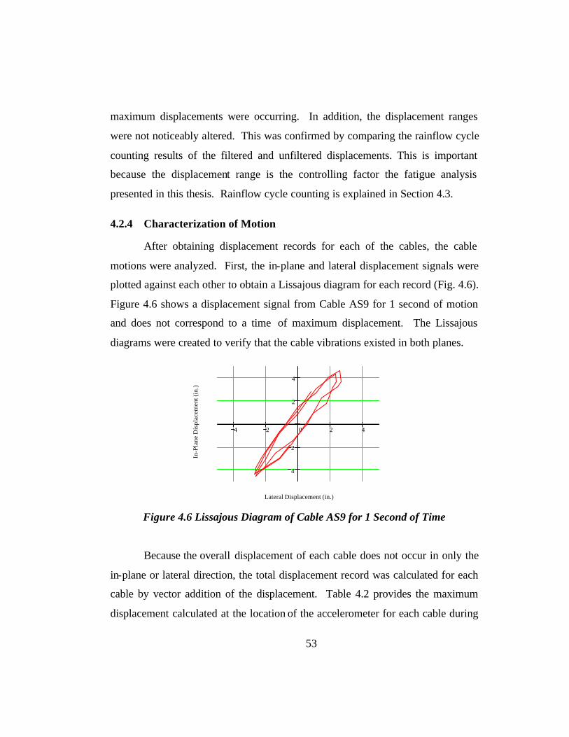
Data from JHU is used to characterize the cable motions in Chapter 4 of
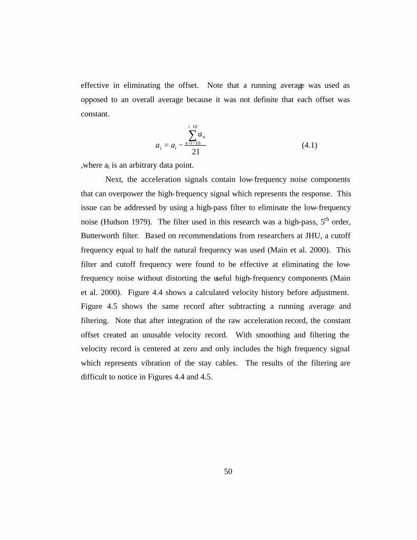
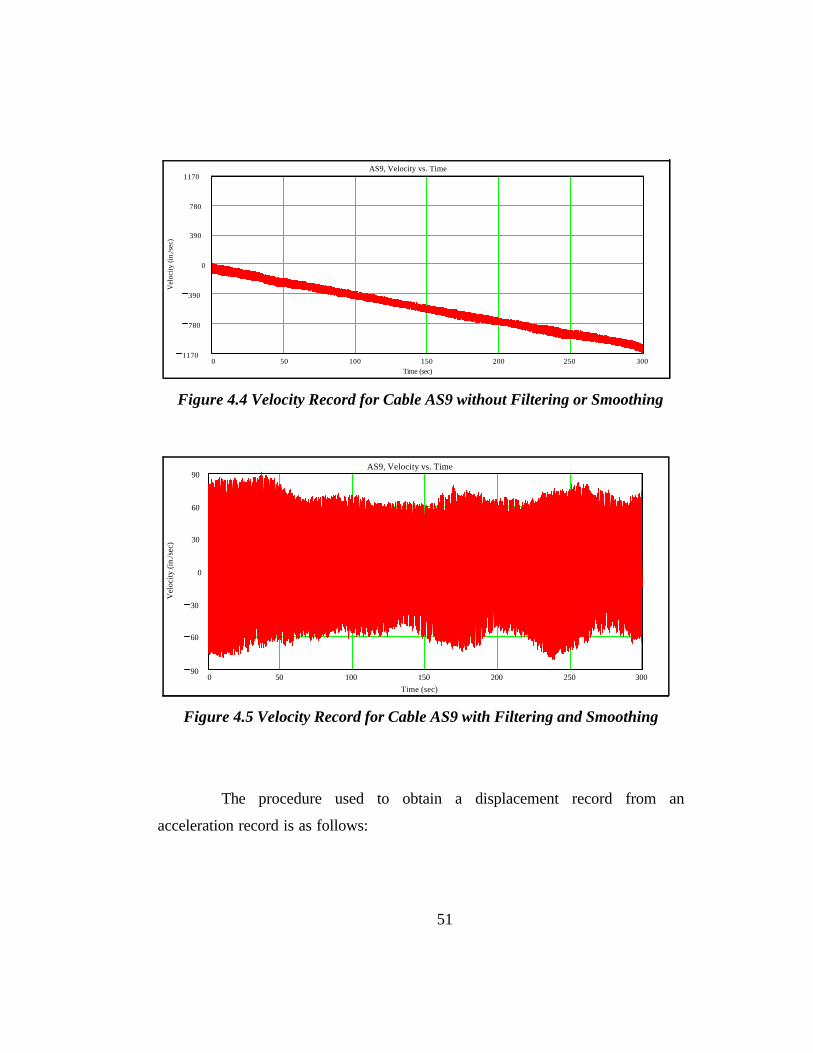
this thesis. Acceleration data from wind-rain vibration events are used to
calculate the displacement history during ten different wind-rain events. The
displacement histories are used to characterize the vibration of the cables in terms
of Lissajous diagrams and mode number.
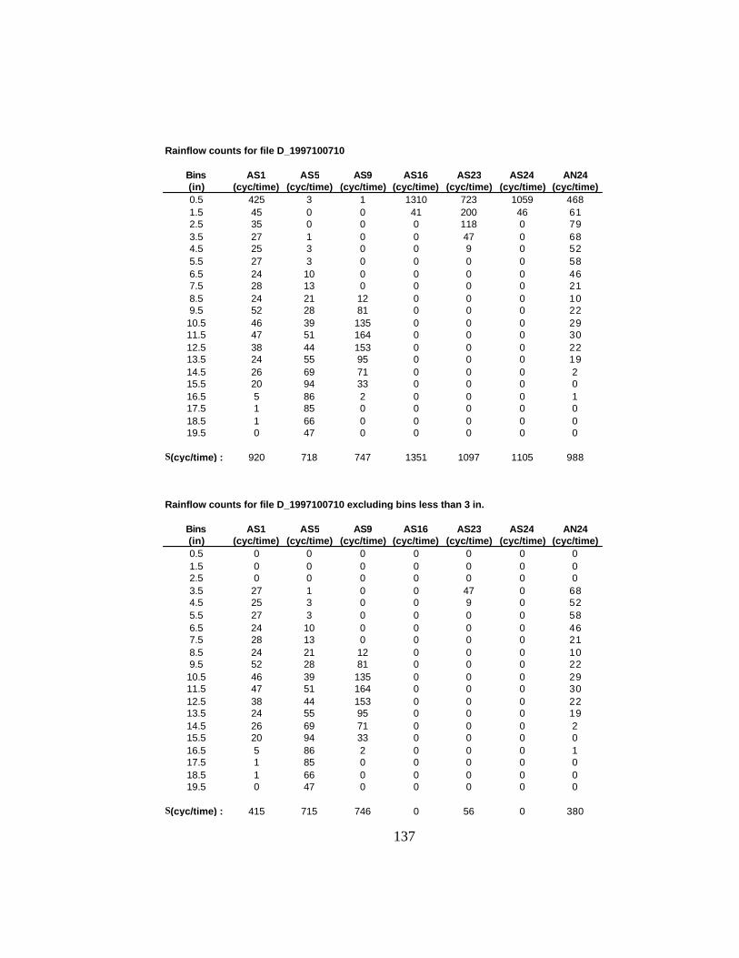
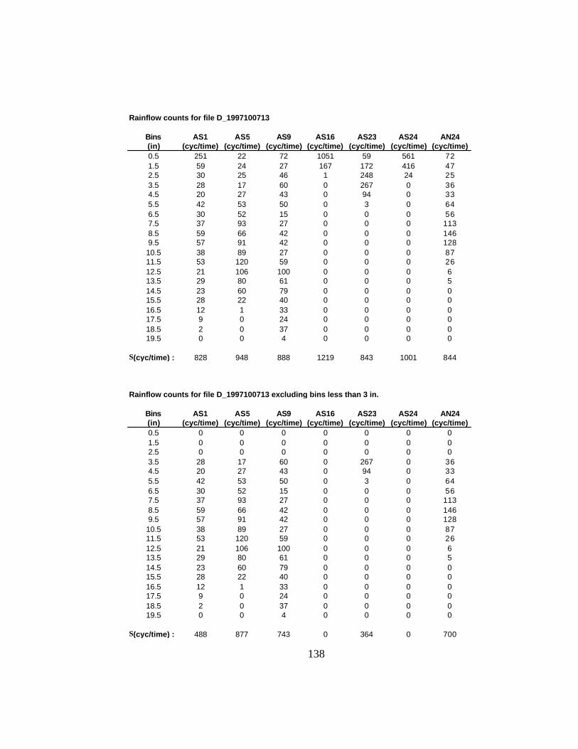
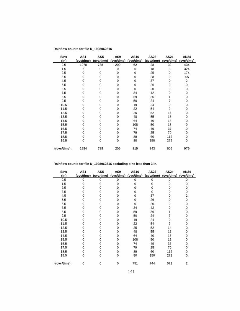
The displacement histories for each cable are characterized using rainflow
counting and the results are used to develop an equivalent displacement for each
cable. Next, statistical data compiled by researchers at JHU are used to estimate
the amount of time that each of the cables has experienced wind-rain induced
vibrations. These results are compared with the observed fatigue life of the first
five stay cable specimens.
The result s of the vibration characterization are in the form of an
equivalent displacement at the location of the accelerometer and an estimated
number of cycles that the cable has experienced since construction. After
refinement of the computational model, the research team should be able to use
9
the results of the cable fatigue characterization and the cable stay tests to estimate
fatigue damage and the remaining life of the stay cables that support the Fred
Hartman Bridge.
10
CHAPTER 2
Single-strand Bending Tests
This chapter explains the development of simplified closed-form solutions
for single-strand bending and describes the testing of single 0.6- in., 7-wire strand
under tension and bending.
2.1 INTRODUCTION
Analysis of stay cables under tension and bending loads is a complex
problem. The interactions between the grout and strands and the relative
movement of the wires within each strand are not fully understood. Previously on
this project, analysis and testing of full-scale cable specimens was performed
(Dowd 2001, Poser 2001). The full-scale specimens were 19-strand cables, 33
feet in length and similar in design to cables constructed on the Fred Hartman
Bridge. Each was pre-stressed to 40 percent of the guaranteed ultimate strength
and bending was induced by imposing a mid-span deflection.
Dowd (2001) developed a finite element model of the full-scale strand
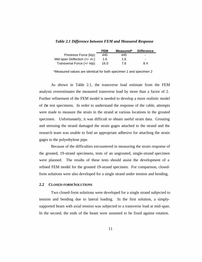
specimen using beam elements and transformed sections. Table 2.1 shows a
comparison of the transverse load calculated using that FEM model for a mid-
span deflection of 1.6 in. (Dowd 2001) and the measured transverse load for
specimens one and two for a mid-span deflection of 1.6 in. (Poser 2001).
11
Table 2.1 Difference between FEM and Measured Response
FEM Measured* DifferencePrestress Force (kip): 445 445 -
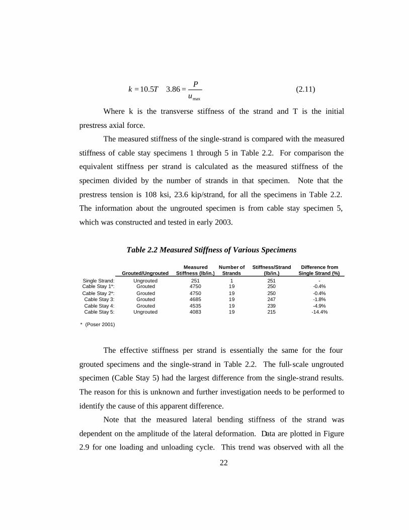
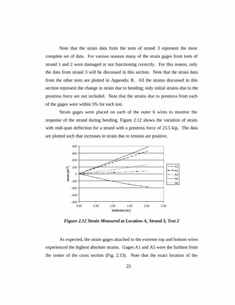
Note that all the test specimens experienced a relatively high number of
cycles compared to the bridge cables but the amount of displacement and the
location of the displacements are not the same for both the specimens and the
bridge cables. It is important to note that all of the cables in Table 4.10 are larger
in diameter and have more strands than the 19-strand test specimen. Because of
this difference, the stress induced by the same displacement will be higher in the
bridge cables for the same displacement. Because the FEM models developed on
this project are not able to correlate the displacement of a cable to the stress at the
ends, there is no way to compare these results. Future FEM models should be
able to estimate the stresses in any size cable based on a given displacement and
displacement location. It is anticipated that future researchers will be able to
evaluate the fatigue damage based on a refined FEM model and the results
presented in this chapter.
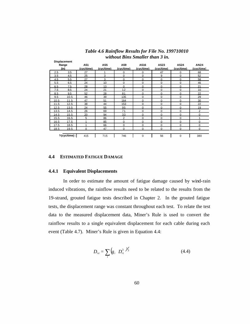
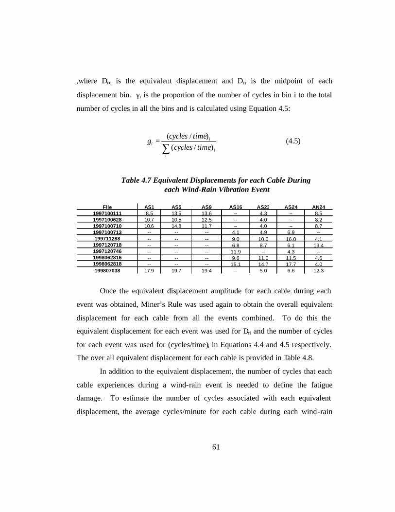
4.6 RECOMMENDATION FOR FUTURE RESEARCH
Further research needs to be performed to verify the results of this chapter.
The equivalent displacement and cycles/minute are based on a limited number of
records and should include more records of wind-rain induced vibration. To do
this the process should be automated to improve efficiency. In addition the
65
analysis should include all of the cables that were instrumented with
accelerometers so the results can be more easily applied to all the cables on the
bridge.
Another improvement for the analysis would be to analyze each one-
minute segment included in the JHU database. While this may be an arduous
task, it would lead to a much more accurate estimate of the amount of time each
cable has undergone wind-rain induced vibrations. The more accurate estimate
should be less than the estimate presented in this chapter and should also provide
a better confidence level.
When a refined FEM model is complete, these results should be analyzed.
When the stress in the Fred Hartman cables is better understood, the 19-strand
tests can be modified to better resemble the stresses in the bridge cables. In
addition, the results presented in this chapter can be used to estimate the fatigue
damage of each bridge cable due to wind-rain induced vibrations.
66
CHAPTER 5
Summary and Conclusions
This thesis was prepared to assist the research team with the fatigue
analysis of the Fred Hartman Bridge stay cables. While this thesis does not report
the results of any full-scale cable tests, it does provide information to assist the
research team with future research. The three topics discussed in this thesis
include:
1. Static tests of single-strand specimens under tension and bending
and the development of the associated closed-form solutions for a
simply-supported beam and a fixed-fixed beam. The results of the
single-strand test are compared with the 19-strand specimens and
the closed-form solutions.
2. Tensile fatigue testing of representative strand used to construct
the full-scale specimens 1 through 6. The results are compared
with published strand fatigue data and PTI specifications.
3. Characterization of the cable stay vibration data from the Fred
Hartman Bridge. The vibration data were used to estimate the
fatigue damage to the Fred Hartman cables due to wind-rain
induced vibration.
5.1 SINGLE-STRAND BENDING TESTS
The single-strand bending tests provided information about the bending
characteristics of single-strand specimens under tension. The results of these tests
67
and the associated closed-form solutions should assist the research team with
improving the FEM models for the 19-strand specimen. Important information
obtained with these tests includes:
o The strain due to bending is essentially zero 12 in. from the face of
the chuck, which agrees with the closed-form solution, for a fixed-
fixed beam.
o Based on the stiffness comparison between the single-strand tests
and grouted and ungrouted 19-strand tests, it appears that the grout
has only a minor influence on the stiffness of the 19-strand
specimens.
o The single-strand specimens were approximately 2% less stiff than
the stiffness calculated using the closed form solution for a fixed-
fixed beam and approximately 4% more stiff than the stiffness
calculated using the closed-form solution for a simply-supported
beam. This concludes that the two models are upper and lower
bounds to the actual stiffness of the strand.
o The measured response of individual single-strand indicated that
the single-strand specimen became slightly stiffer as mid-point
deflection increased. The most probable reason for the increase in
stiffness is an increase in tension during bending. This
phenomenon was not considered in the closed-form solution.
o An effective EI of 0.94EI can be used in the fixed-fixed beam
solution to attain the observed response of a single strand.
o Based on the moment comparison between the single-strand tests
and the closed-form solutions, it appears that the calculated
68
moment in the strand is less than the closed form solution for the
fixed-fixed beam.
5.2 STRAND TENSION FATIGUE TESTS
The strand tension fatigue tests were used to develop the fatigue
characteristics of the strand used to construct Stay Cable Tests 1 through 6.
Results of the tests indicate that the fatigue characteristic of the strand do not meet
the 1986 or the 2001 PTI specifications. The strand however does fall between
the minimum and mean of strand fatigue data published by Paulson (1983).
Recommendations for the strand tension fatigue tests include:
o Additional strand fatigue tests should be performed at stress ranges
other than 20, 30, and 40 ksi. to develop a complete S-N curve for
the strand
o When the stress in the strands of the 19-strand specimens is better
defined, strand fatigue tests should be performed at those stress
ranges. With the additional information from these tests, the
failure mechanism of the wires in the 19-strand specimens and
hence the Fred Hartman bridge should be better understood.
o A test should be developed to conduct fatigue tests of grouted
single strands. These results will assist in the identification of
fretting and the associated reduction in fatigue life due to fretting.
5.3 FRED HARTMAN CABLE VIBRATION CHARACTERIZATION
Acceleration records from cable vibration events on the Fred Hartman
Bridge were characterized in terms of the following characteristics:
69
o The displacement of cable at the accelerometer location
o Primary vibration frequencies and mode of the cable vibration
o The equivalent displacement and the associated cycles/minute for
each cable
o The total number of cycles that each cable has undergone since
construction of the bridge in September of 1995.
After characterization of the cable stay vibrations the calculated
displacement record was used to estimate the equivalent displacement of each
bridge cable analyzed. Using the database developed by researchers at Johns
Hopkins the total number of cycles that each cable experienced was also
estimated. It is not possible to relate these results to fatigue damage because of
the differences in calculated displacement location and cable size. However, it
was concluded that a refined FEM model needs to be developed to relate the
deflection of the cables to stress at the ends. With this refined model, the results
presented in Chapter 4 can be used to evaluate the fatigue damage in the Fred
Hartman stay-cables.
The following are recommendations for improving this analysis:
o More than ten wind-rain vibrations records should be
characterized. If possible, the process should be automated for
efficiency. In addition, all the cables that had accelerometers
should be included in the analysis.
o The one-minute acceleration records from the database should be
analyzed for a better prediction of the total number of cycles that
each cable has undergone. This process should also be automated
to improve efficiency.
70
o After the refined FEM model is complete, the stresses in the Fred
Hartman cables should be estimated so that the 19-strand tests can
be adjusted to simulate the bending stresses seen in the bridge
cables. The results of these improved tests should provide better
estimates of the actual fatigue damage.
108
Appendix A
Closed-Form Solutions
The derivation of both closed-form solutions were developed with the
following parameters:
o The strand is viewed as a tension strut with a transverse force at mid-
span
o To include secondary bending effects due to the tension in the strand,
the free-body diagram (FBD) includes an initial deflection due to the
transverse load. This is similar to the derivation of a compression
member with secondary bending (i.e. Euler buckling), except the
solution is stable due to the tension in the strand.
o Deformation due to shear was ignored due to the large span-to-depth
ratio of the strand.
o Because the transverse load is located at mid-span, the solutions for
both cases are symmetric. Therefore the solutions are derived for only
half of the beam.
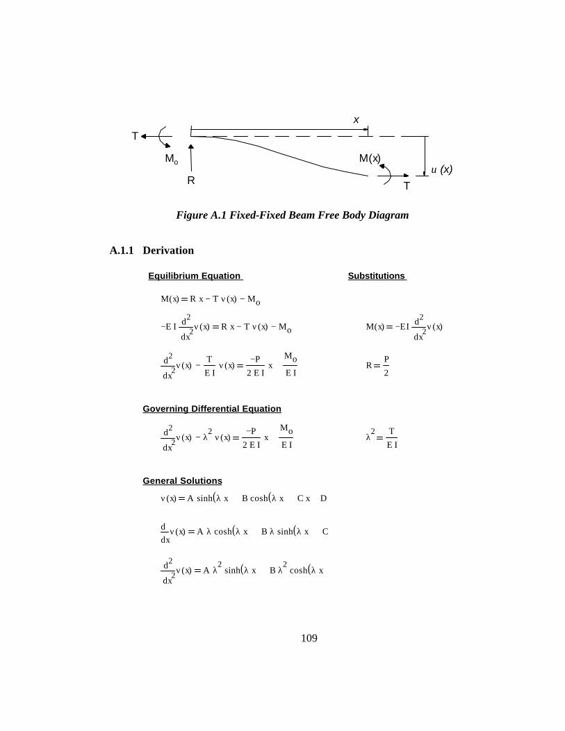
A.1 FIXED-FIXED BEAM WITH AXIAL TENSION AND BENDING
Figure A.1 shows the free body diagram used to establish the equilibrium
equation for the fixed-fixed beam. The equilibrium equation is developed by
summing the moments about an arbitrary point at a distance x, along the beam.
109
Figure A.1 Fixed-Fixed Beam Free Body Diagram
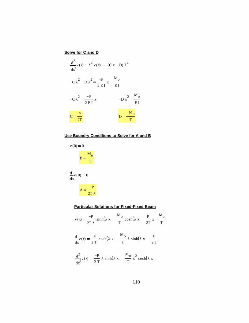
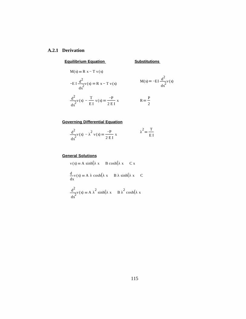
A.1.1 Derivation
Equilibrium Equation Substitutions
M x( ) R x⋅ T ν x( )⋅− Mo−
E− I⋅ 2x
ν x( )d
d
2⋅ R x⋅ T ν x( )⋅− Mo− M x( ) E− I 2
xν x( )d
d
2⋅
2x
ν x( )d
d
2 T
E I⋅ν x( )⋅−
P−
2 E⋅ I⋅x⋅
Mo
E I⋅+ R
P
2
Governing Differential Equation
2x
ν x( )d
d
2λ
2ν x( )⋅−
P−
2 E⋅ I⋅x⋅
Mo
E I⋅+ λ
2 T
E I⋅
General Solutions
ν x( ) A sinh λ x⋅( )⋅ B cosh λ x⋅( )⋅+ C x⋅+ D+
xν x( )d
dA λ⋅ cosh λ x⋅( )⋅ B λ⋅ sinh λ x⋅( )⋅+ C+
2x
ν x( )d
d
2A λ
2⋅ sinh λ x⋅( )⋅ B λ
2⋅ cosh λ x⋅( )⋅+
T
TR
Mo M(x)
x
υ (x)
110
Solve for C and D
2x
ν x( )d
d
2λ
2ν x( )⋅− C x⋅ D+( )− λ
2⋅
C− λ2
⋅ D λ2
⋅−P−
2 E⋅ I⋅x⋅
Mo
E I⋅+
C− λ2
⋅P−
2 E⋅ I⋅x⋅ D− λ
2⋅
Mo
E I⋅
CP
2TD
Mo−
T
Use Boundry Conditions to Solve for A and B
ν 0( ) 0
BMo
T
xν 0( )d
d0
AP−
2T λ⋅
Particular Solutions for Fixed-Fixed Beam
ν x( )P−
2T λ⋅sinh λ x⋅( )⋅
Mo
Tcosh λ x⋅( )⋅+
P
2Tx⋅+
Mo
T−
xν x( )d
d
P−
2 T⋅cosh λ x⋅( )⋅
Mo
Tλ⋅ sinh λ x⋅( )⋅+
P
2 T⋅+
2x
ν x( )d
d
2 P−
2 T⋅λ⋅ sinh λ x⋅( )⋅
Mo
Tλ
2⋅ cosh λ x⋅( )⋅+
111
Solve for Mo
since load is at mid-span,
Mo ML
2
and,
xν
L
2
dd
0
MoP L⋅
2
coshL
2λ⋅
1−
sinhL
2λ⋅
⋅
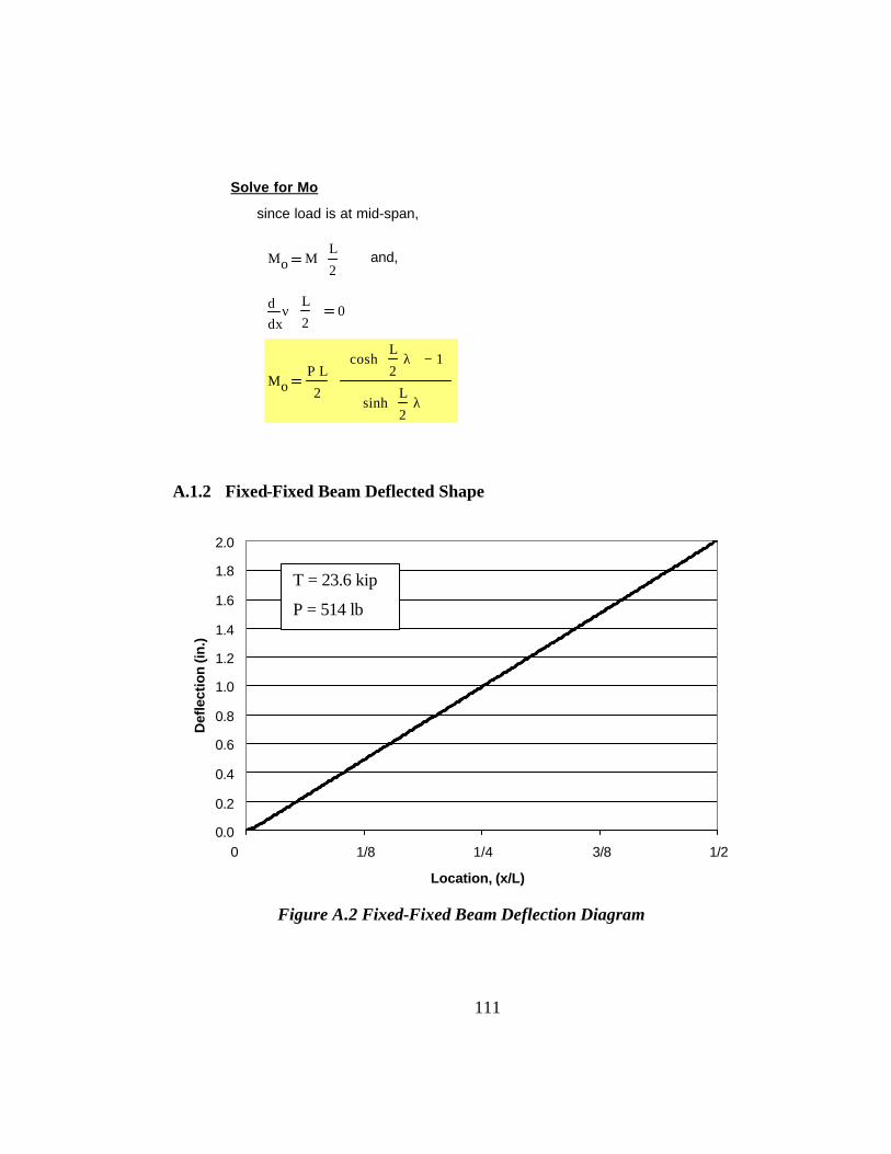
A.1.2 Fixed-Fixed Beam Deflected Shape
0.0
0.2
0.4
0.6
0.8
1.0
1.2
1.4
1.6
1.8
2.0
0 1/8 1/4 3/8 1/2
Location, (x/L)
Def
lect
ion
(in
.)
Figure A.2 Fixed-Fixed Beam Deflection Diagram
T = 23.6 kip
P = 514 lb
112
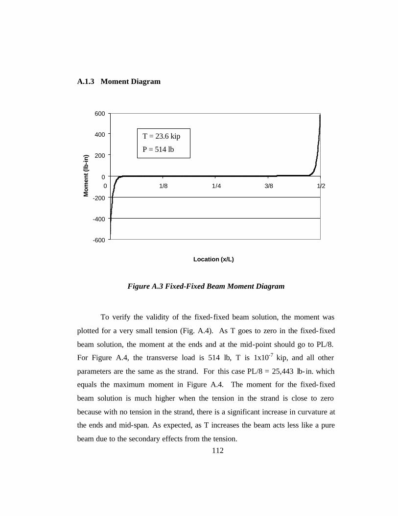
A.1.3 Moment Diagram
-600
-400
-200
0
200
400
600
0 1/8 1/4 3/8 1/2
Location (x/L)
Mom
ent (
lb-in
)
Figure A.3 Fixed-Fixed Beam Moment Diagram
To verify the validity of the fixed-fixed beam solution, the moment was
plotted for a very small tension (Fig. A.4). As T goes to zero in the fixed-fixed
beam solution, the moment at the ends and at the mid-point should go to PL/8.
For Figure A.4, the transverse load is 514 lb, T is 1x10⁻⁷ kip, and all other
parameters are the same as the strand. For this case PL/8 = 25,443 lb- in. which
equals the maximum moment in Figure A.4. The moment for the fixed-fixed
beam solution is much higher when the tension in the strand is close to zero
because with no tension in the strand, there is a significant increase in curvature at
the ends and mid-span. As expected, as T increases the beam acts less like a pure
beam due to the secondary effects from the tension.
T = 23.6 kip
P = 514 lb
113
-30,000
-20,000
-10,000
0
10,000
20,000
30,000
0 1/8 1/4 3/8 1/2
Location (x/L)
Mom
ent
(lb-in
)
Figure A.4 Fixed-Fixed Beam Moment Diagram for T ˜ 0 kip
T = 0 kip
P = 514 lb
114
A.2 SIMPLY SUPPORTED BEAM WITH AXIAL TENSION AND BENDING
Figure A.4 shows the free body diagram used to develop the equilibrium
equation for the simply-supported solution. The primary difference between the
fixed-fixed solution and the simply-supported solution is the reaction moment at
the beam ends. The deflection diagram (Fig. A.4) and the moment diagram (Fig.
A.6) are associated with a transverse load of 482 lb which results in a stiffness of
241 lb/in.
Figure A.5 Simply-Supported Beam Free Body Diagram
T
TR
M(x)
x
υ (x)
115
A.2.1 Derivation
Equilibrium Equation Substitutions
M x( ) R x⋅ T ν x( )⋅−
M x( ) E− I 2x
ν x( )d
d
2⋅
E− I⋅ 2x
ν x( )d
d
2⋅ R x⋅ T ν x( )⋅−
2x
ν x( )d
d
2 T
E I⋅ν x( )⋅−
P−
2 E⋅ I⋅x⋅ R
P
2
Governing Differential Equation
λ2 T
E I⋅2x
ν x( )d
d
2λ
2ν x( )⋅−
P−
2 E⋅ I⋅x⋅
General Solutions
ν x( ) A sinh λ x⋅( )⋅ B cosh λ x⋅( )⋅+ C x⋅+
xν x( )d
dA λ⋅ cosh λ x⋅( )⋅ B λ⋅ sinh λ x⋅( )⋅+ C+
2x
ν x( )d
d
2A λ
2⋅ sinh λ x⋅( )⋅ B λ
2⋅ cosh λ x⋅( )⋅+
116
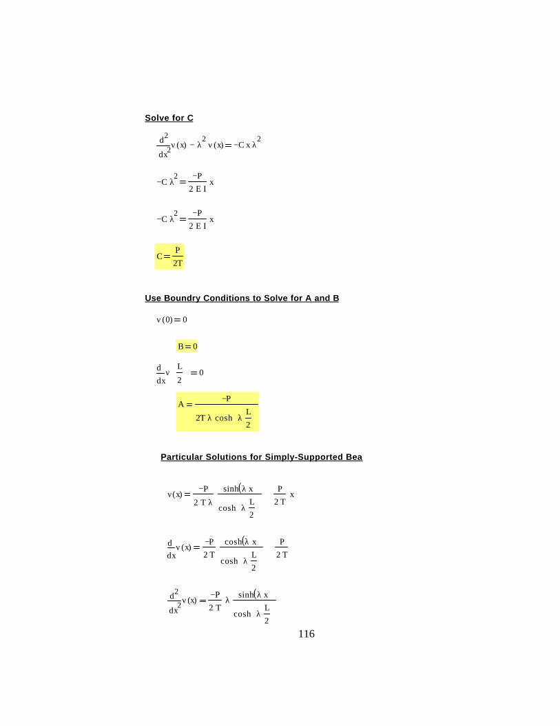
Solve for C
2xν x( )d
d
2λ
2ν x( )⋅− C− x⋅ λ
2⋅
C− λ2
⋅P−
2 E⋅ I⋅x⋅
C− λ2
⋅P−
2 E⋅ I⋅x⋅
CP2T
Use Boundry Conditions to Solve for A and B
ν 0( ) 0
B 0
xν
L
2
dd
0
AP−
2T λ⋅ cosh λL2
⋅
⋅
Particular Solutions for Simply-Supported Beam
ν x( )P−
2 T⋅ λ⋅
sinh λ x⋅( )
cosh λL2
⋅
⋅P
2 T⋅x⋅+
xν x( )d
d
P−2 T⋅
cosh λ x⋅( )
cosh λL2
⋅
⋅P
2 T⋅+
2x
ν x( )d
d
2 P−2 T⋅
λ⋅sinh λ x⋅( )
cosh λL2
⋅
⋅
117
A.2.2 Simply-Supported Beam Defected Shape
Figure A.6 shows the deflected shape for a simply-supported beam with a
tension of 23.6 kip and a transverse load at the midpoint of 482 lb. This correlates
to a maximum deflection of 2.0 in.
0.0
0.2
0.4
0.6
0.8
1.0
1.2
1.4
1.6
1.8
2.0
0 1/8 1/4 3/8 1/2
Location (x/L)
Def
lect
ion
(in)
Figure A.6 Simply-Supported Deflected Shape
T = 23.6 kip
P = 482 lb
118
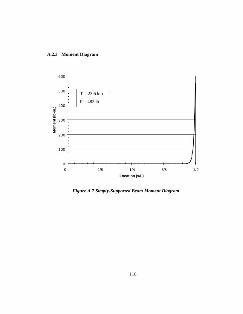
A.2.3 Moment Diagram
0
100
200
300
400
500
600
0 1/8 1/4 3/8 1/2
Location (x/L)
Mom
ent (
lb-in
.)
Figure A.7 Simply-Supported Beam Moment Diagram
T = 23.6 kip
P = 482 lb
119
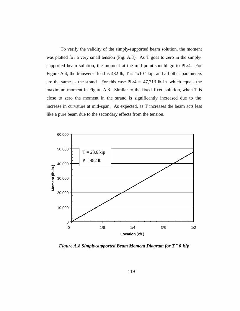
To verify the validity of the simply-supported beam solution, the moment
was plotted for a very small tension (Fig. A.8). As T goes to zero in the simply-
supported beam solution, the moment at the mid-point should go to PL/4. For
Figure A.4, the transverse load is 482 lb, T is 1x10⁻⁷ kip, and all other parameters
are the same as the strand. For this case PL/4 = 47,713 lb- in. which equals the
maximum moment in Figure A.8. Similar to the fixed-fixed solution, when T is
close to zero the moment in the strand is significantly increased due to the
increase in curvature at mid-span. As expected, as T increases the beam acts less
like a pure beam due to the secondary effects from the tension.
0
10,000
20,000
30,000
40,000
50,000
60,000
0 1/8 1/4 3/8 1/2
Location (x/L)
Mom
ent (
lb-in
.)
Figure A.8 Simply-supported Beam Moment Diagram for T ˜ 0 kip
T = 23.6 kip
P = 482 lb
120
Appendix B
Single-Strand Bending Tests
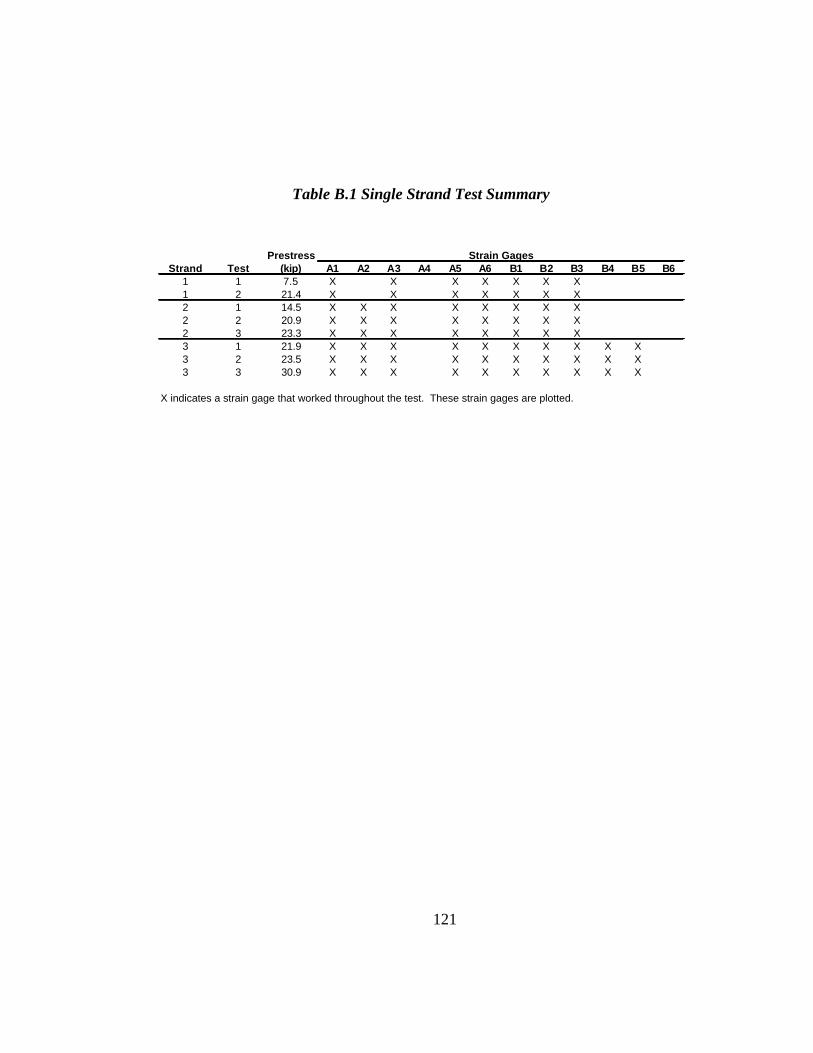
The single-strand bending tests were performed with three different strand
specimens. For each specimen two or three tests were performed at different
prestress levels. Note that each test was repeated at least twice. Only one cycle
of each test is included in this appendix because the responses of the tests were
within 5 % of each other for each cycle. Also note that tests performed at low
prestress levels (less than 4 kip) are not included in this appendix because the
variation in strain was extremely small.
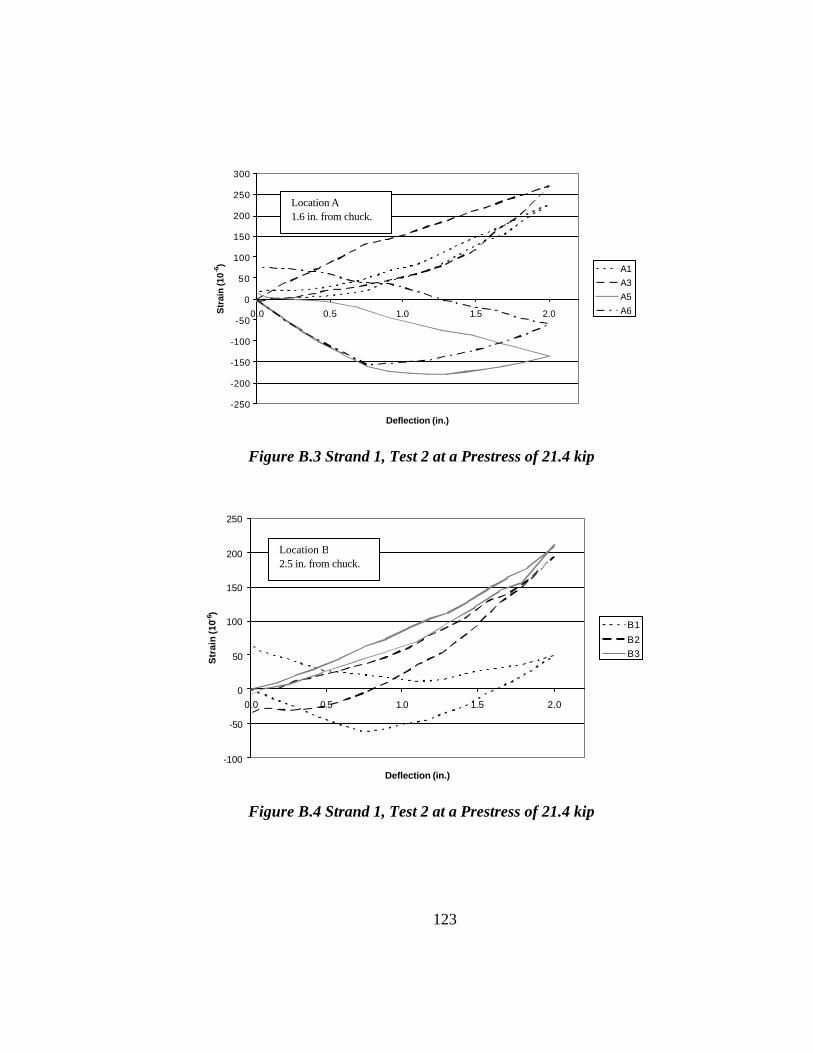
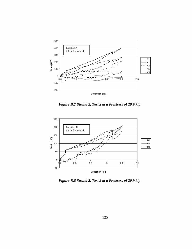
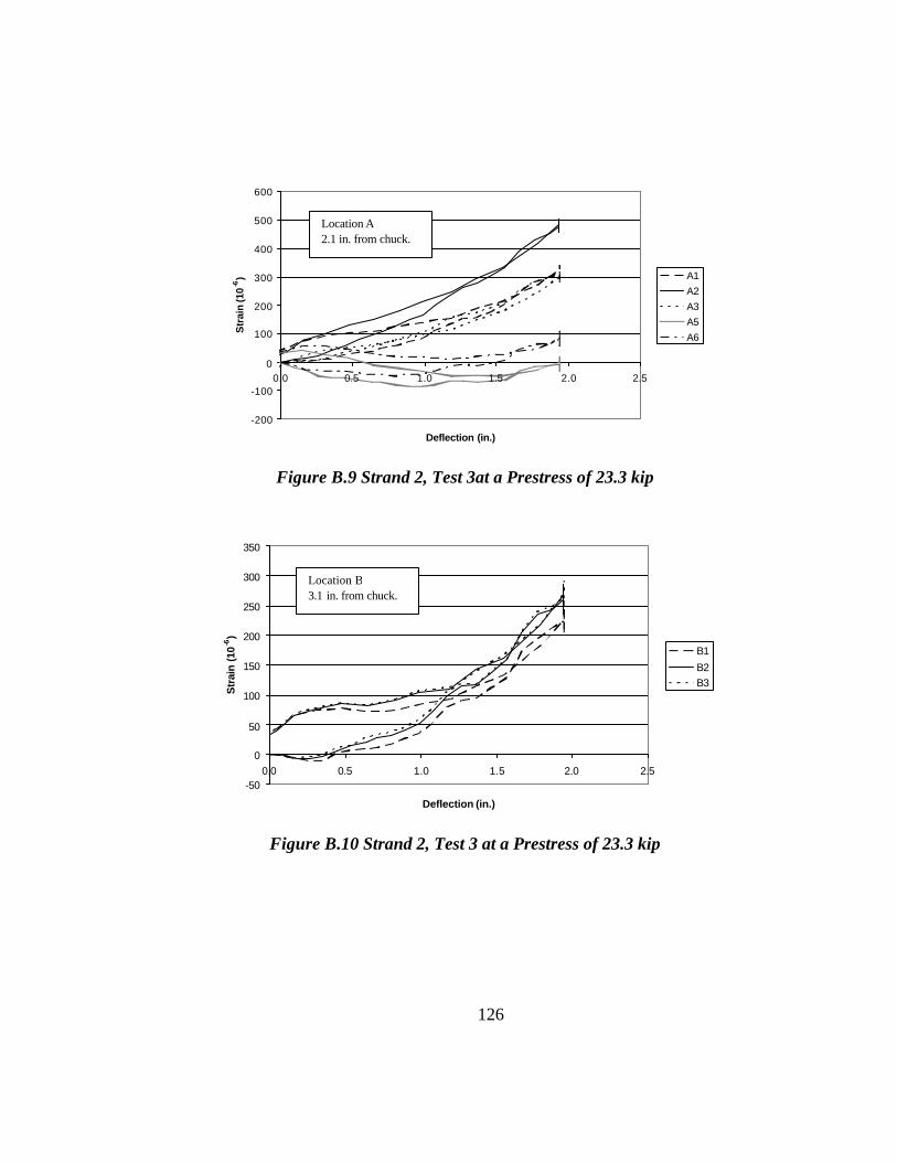
Strains measured by all functioning gages are plotted against mid-span
deflection of the strand in this appendix. Note that at least one of the strain gages
failed to yield useful data due to damage or de-bonding from the strand in all the
tests. Data from these gages are not plotted. The strand specimen number and the
test number are indicated in the title of each plot and the gage location is indicated
within each plot. Table B.1 provides a summary of the tests and indicates which
strain gage data was plotted for each test.
Also included in this appendix is a copy of the manufacturer’s
specification sheet for the strand used in the single-strand bending tests, the strand
tension fatigue tests, and the full-sized stay-cable bending fatigue tests
(Fig. B.17).
In addition, this appendix includes data collected for verification of the
size of the strand. For a strand sample, the area of each wire was measured and
tabula ted (Fig. B.18).
121
Table B.1 Single Strand Test Summary
Prestress
Strand Test (kip) A1 A2 A3 A4 A5 A6 B1 B2 B3 B4 B5 B61 1 7.5 X X X X X X X1 2 21.4 X X X X X X X2 1 14.5 X X X X X X X X2 2 20.9 X X X X X X X X2 3 23.3 X X X X X X X X3 1 21.9 X X X X X X X X X X3 2 23.5 X X X X X X X X X X3 3 30.9 X X X X X X X X X X
X indicates a strain gage that worked throughout the test. These strain gages are plotted.
Strain Gages
122
-80
-60
-40
-20
0
20
40
60
80
100
120
0.0 0.5 1.0 1.5 2.0
Deflection (in.)
Str
ain
(10-6
) A1A3A5A6
Figure B.1 Strand 1, Test 1 at a Prestress of 7.5 kip
-40
-20
0
20
40
60
80
0.0 0.5 1.0 1.5 2.0
Deflection (in.)
Str
ain
(10
-6)
B1
B2B3
Figure B.2 Strand 1, Test 1 at a Prestress of 7.5 kip
Location B 2.5 in. from chuck.
Location A 1.6 in. from chuck.
123
-250
-200
-150
-100
-50
0
50
100
150
200
250
300
0.0 0.5 1.0 1.5 2.0
Deflection (in.)
Str
ain
(10
-6) A1
A3A5A6
Figure B.3 Strand 1, Test 2 at a Prestress of 21.4 kip
-100
-50
0
50
100
150
200
250
0.0 0.5 1.0 1.5 2.0
Deflection (in.)
Str
ain
(10-6
)
B1
B2B3
Figure B.4 Strand 1, Test 2 at a Prestress of 21.4 kip
Location A 1.6 in. from chuck.
Location B 2.5 in. from chuck.
124
-60
-40
-20
0
20
40
60
80
100
120
140
0.0 0.2 0.4 0.6 0.8 1.0 1.2 1.4 1.6 1.8 2.0 2.2
Deflection (in)
Str
ain
(10
-6) A1
A2
A3
A5
A6
Figure B.5 Strand 2, Test 1 at a Prestress of 14.5 kip
-20
-10
0
10
20
30
40
50
60
0.0 0.2 0.4 0.6 0.8 1.0 1.2 1.4 1.6 1.8 2.0 2.2
Deflection (in)
Str
ain
(10-6
)
B1
B2
B3
Figure B.6 Strand 2, Test 1 at a Prestress of 14.5 kip
Location A 2.1 in. from chuck.
Location B 3.1 in. from chuck.
125
-200
-100
0
100
200
300
400
500
0.0 0.5 1.0 1.5 2.0 2.5
Deflection (in.)
Str
ain
(10-6
) A1A2A3A5A5
Figure B.7 Strand 2, Test 2 at a Prestress of 20.9 kip
-50
0
50
100
150
200
250
0.0 0.5 1.0 1.5 2.0 2.5
Deflection (in.)
Str
ain
(10-6
)
B1B2B3
Figure B.8 Strand 2, Test 2 at a Prestress of 20.9 kip
Location A 2.1 in. from chuck.
Location B 3.1 in. from chuck.
126
-200
-100
0
100
200
300
400
500
600
0.0 0.5 1.0 1.5 2.0 2.5
Deflection (in.)
Str
ain
(10
-6) A1
A2A3A5A6
Figure B.9 Strand 2, Test 3at a Prestress of 23.3 kip
-50
0
50
100
150
200
250
300
350
0.0 0.5 1.0 1.5 2.0 2.5
Deflection (in.)
Str
ain
(10
-6)
B1
B2B3
Figure B.10 Strand 2, Test 3 at a Prestress of 23.3 kip
Location A 2.1 in. from chuck.
Location B 3.1 in. from chuck.
127
-300
-200
-100
0
100
200
300
400
500
0 0.5 1 1.5 2 2.5
Deflection (in.)
Str
ain
(10
-6) A1
A2
A3
A5
A6
Figure B.11 Strand 3, Test 1 at a Prestress of 21.9 kip
-20
0
20
40
60
80
100
120
0 0.5 1 1.5 2 2.5
Deflection (in.)
Str
ain
(10-6
) B1
B2
B3
B4
B5
Figure B.12 Strand 3, Test 1 at a Prestress of 21.9 kip
Location A 1.8 in. from chuck.
Location B 2.5 in. from chuck.
128
-400
-300
-200
-100
0
100
200
300
400
0.00 0.50 1.00 1.50 2.00 2.50
Deflection (in.)
Str
ain
(10
-6) A1
A2A3
A5A6
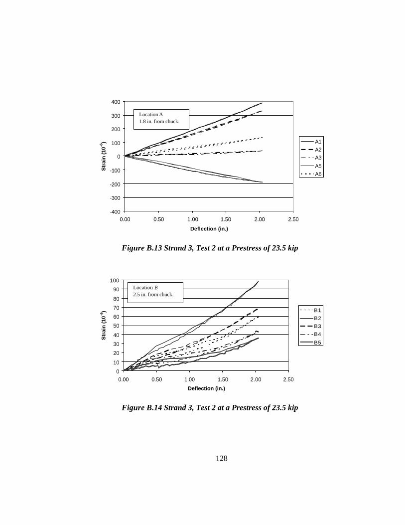
Figure B.13 Strand 3, Test 2 at a Prestress of 23.5 kip
0
10
20
30
40
50
60
70
80
90
100
0.00 0.50 1.00 1.50 2.00 2.50
Deflection (in.)
Str
ain
(10-6
) B1B2B3B4
B5
Figure B.14 Strand 3, Test 2 at a Prestress of 23.5 kip
Location A 1.8 in. from chuck.
Location B 2.5 in. from chuck.
129
-300
-200
-100
0
100
200
300
400
500
0 0.5 1 1.5 2 2.5
Deflection (in.)
Str
ain
(10
-6) A1
A2A3A5A6
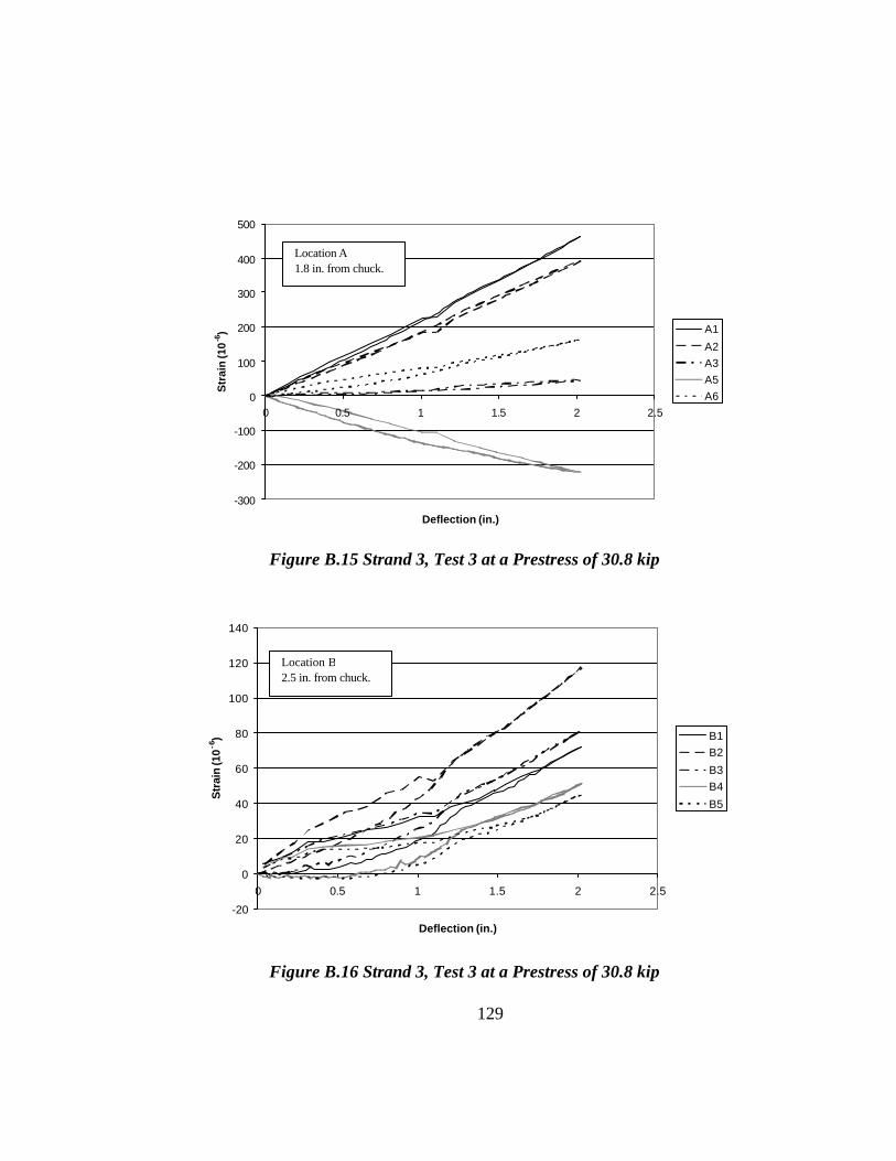
Figure B.15 Strand 3, Test 3 at a Prestress of 30.8 kip
-20
0
20
40
60
80
100
120
140
0 0.5 1 1.5 2 2.5
Deflection (in.)
Str
ain
(10
-6) B1
B2
B3B4
B5
Figure B.16 Strand 3, Test 3 at a Prestress of 30.8 kip
Location A 1.8 in. from chuck.
Location B 2.5 in. from chuck.
130
Figure B.17 Strand Specification Sheet
131
A sample strand was used to measure the area of each wire to verify the
size of the strand used in the single strand tests and the full-scale specimens 1
through 6. The measure the area of each wire, the sample strand was unwound
into 7 separate wires. Each wire was measured to be 6 1/16-in. long. Each wire
was placed in a graduated cylinder filled with water. The displacement of each
wire was recorded and the area of each wire was ten calculated (Fig. B.18). The
total measured area of the strand was essentially the same as the area provided by
ASTM E 1049-85 (1985), “Standard Practices for Cycle Counting in Fatigue Analysis,” American Society for Testing and Materials, West Conshohocken, PA, Reapproved 1999.
Buhl M. (2002), “CRUNCH Users Manual,” National Wind Technology Center at the National Renewable Energy Laboratory, Golden, Colorado
Downing, S. D. and Socie, D. F. (1982), “Simple Rainflow Counting Algorithms,” International Journal of Fatigue, Vol. 4, No. 1, pp. 31-40.
Hudson, D. E. (1979), “Reading and Interpreting Strong Motion Accelerograms,” Earthquake Engineering Research Institute, Engineering Monograph No. 1, Berkeley, CA.
Lamb, J. L. (1985), “Study of Simple Fatigue Resistant Anchorage for Cable-Stayed Applications”, M.S. Thesis, Department of Civil Engineering, The University of Texas at Austin.
Main, J. A. (2000), “Characterization of Rain-Wind Induced Stay-Cable Vibrations from Full-Scale Measurements,” NSF/STA Summer Institute Research Report, Saitama University, Saitama, Japan.
Main, J. A., Jones, N. P., and Yamaguchi, H., (2000), “Characterization of Rain-Wind Induced Stay-Cable Vibrations from Full-Scale Measurements”, Johns Hopkins University, Baltimore, MD and Saitama University, Urawa, Saitama, Japan.
Papailiou, K. O. (1999), “On the Bending of Multi-Layer Strands,” Wire, Vol. 49, No. 5, pp. 44-47.
Paulson, C., Frank, K., and Breen, J. (1983), “A Fatigue Study of Prestressing Strand,” Research Report 300-1, Center for Transportation Research, Bureau of Engineering Research, The University of Texas at Austin, Austin, TX, April 1983.
Poser, Marcel (2001), “Full-Scale Bending Fatigue Tests on Stay Cables”, M.S. Thesis, Department of Civil Engineering, The University of Texas at Austin.
144
Poston, R. W. and Kesner, Keith (1990), “Progress Report Number Two, Evaluation and Repair of Stay-Cable Vibrations, Fred Hartman Bridge, Veterans Memorial Bridge”, Whitlock Dalrymple Poston and Associates, Inc., Manassas, Virginia
PTI Guide Specification (2001), “Recommendations for Stay Cable Design, Testing and Installation”, Post-Tensioning Institute, Phoenix, AZ.
Sarker, P.P., Mehta, K.C., Zhao, Z., (1999), “Aerodynamic Approach to Control Vibrations in Stay-Cables,” Wind Engineering Research Center, Department of Civil Engineering, Texas Tech University, Lubbock, TX.
Timoshenko, S. (1956). "Strength of Materials: Part II - Advanced Theory and Problems," D.Van Nostrand Co., Inc., Princeton, NJ.