Calculating Geometric Properties of Three-Dimensional

Objects from the Spherical Harmonic Representation

Artemy Baxansky and Nahum Kiryati

School of Electrical EngineeringTel Aviv University

Tel Aviv 69978, Israel

Abstract

The volume, location of the centroid, and second order moments of a three-dimensional star-shaped object are determined in terms of the spherical harmoniccoefficients of its boundary function. Bounds on the surface area of the object are de-rived in terms of the spherical harmonic coefficients as well. Sufficient conditions underwhich the moments and area computed from the truncated spherical harmonic seriesconverge to the actual moments and area are established. The proposed method is ver-ified using a scanned head model and by recent measurements of the 433 Eros asteroid.An extension to non-star-shaped objects of genus 0 is provided. The computationalcomplexity of our method is shown to be equal to that of the discrete spherical har-monic transform, which is O(N2 log2

N), where N is the maximum order of coefficientsretained in the expansion.

1 Introduction

Three-dimensional objects can be represented by surface based descriptions, such as triangu-

lar meshes, or by volume based descriptions, such as voxels. These representations, however,

are based on huge lists of voxels or surface elements. For purposes of image processing and

analysis, the need for a more compact shape representation is important.

Most of this paper is concerned with a limited class of objects called star-shaped.

These have the property that there exists a point in the interior of the object from which

the whole object is ”visible”. In this case we can describe the surface of the object using

standard spherical coordinates r = r(θ, φ). Then r can be arbitrarily well approximated in

1

the basis of spherical harmonics [3]. Usually the global shape can be captured with a small

set of coefficients. It is worth noting that the concept of spherical harmonic representation

has been generalized to non-star-shaped objects ([1] and references therein).

The spherical harmonic technique was used to model the heart [18], to approximate

molecular orbital surfaces and to compute surface shape properties [6]. Garboczi [8] applied

it to characterize aggregate particles in concrete. Spherical harmonics have been also used

recently to characterize the shape of an asteriod [20]. In geodesy, they are used to study

the shape of the earth and the shape of satellite orbits [10]. In computer vision and graph-

ics, the spherical harmonic representation is the basis for 3D shape matching and retrieval

methods [11].

Many applications require the extraction of image-domain features, such as low-order

moments and surface area. For example, content-based 3D model retrieval algorithms based

on moments have been proposed ([17] and references therein). A possiblity to extract the

features directly from the compact representation eliminates the need for prior image recon-

struction and may reduce computational complexity. In [13] properties of two-dimensional

objects were calculated directly from the Fourier-serier coefficients of the boundary function

r(φ). In this work we extend [13] to the three-dimensional case. The main novelty of this

work is that geometric properties are expressed explicitly in terms of the spherical harmonic

coefficients.

This paper is organized as follows. In Section 2 we establish some relations that

will be applied extensively throughout the paper. In Section 3 we obtain expressions for

the moments up to the second order. In Section 4 we develop lower and upper bounds on

the surface area. In section 5 we establish sufficient conditions under which the moments

and area computed from the partial sums of spherical harmonics converge to the actual

2

moments and area. Section 6 is concerned with the simulations we performed to verify the

theoretical results. As one of the examples, we apply our method to calculate the volume

and moments of inertia of the near-Earth asteroid, 433 Eros. In Section 7 we extend our

method to non-star-shaped objects of genus 0. In Section 8 we consider the computational

complexity of the proposed method comparing two approaches: first, the direct evaluation

of a 3D convolution; and second, using the discrete spherical harmonic transform. We show

that the former requires O(N5) operations, as opposed to O(N2 log2 N) for the latter, where

N is the maximum order of coefficients retained in the expansion. Finally, conclusions and

future work are discussed in Section 9.

2 Preliminaries

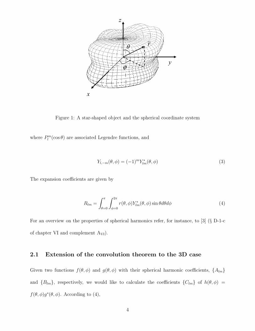
Let ~r describe the radius vector directed from the origin to a boundary point of an object.

We shall work in spherical coordinates that are natural for describing positions on a sphere.

Define φ to be the azimuthal angle between the projection of ~r to the xy-plane and the x-axis

with 0 ≤ φ ≤ 2π, θ to be the polar angle from the z-axis with 0 ≤ θ ≤ π, and r to be the

distance from the point to the origin (see Figure 1). We label the point on the boundary of

the object by its spherical coordinates r, θ, φ. If the function r(θ, φ) is single-valued, such

an object is called star-shaped. r(θ, φ) can be expanded into a series of spherical harmonics:

r(θ, φ) =

∞∑

l=0

l∑

m=−l

RlmYlm(θ, φ) (1)

The spherical harmonics are defined as

Ylm(θ, φ) =

√

2l + 1

4π

(l − m)!

(l + m)!P m

l (cos θ)eimφ (m ≥ 0) (2)

3

Figure 1: A star-shaped object and the spherical coordinate system

where P ml (cos θ) are associated Legendre functions, and

Yl,−m(θ, φ) = (−1)mY ∗lm(θ, φ) (3)

The expansion coefficients are given by

Rlm =

∫ π

θ=0

∫ 2π

φ=0

r(θ, φ)Y ∗lm(θ, φ) sin θdθdφ (4)

For an overview on the properties of spherical harmonics refer, for instance, to [3] (§ D-1-c

of chapter VI and complement AVI).

2.1 Extension of the convolution theorem to the 3D case

Given two functions f(θ, φ) and g(θ, φ) with their spherical harmonic coefficients, Alm

and Blm, respectively, we would like to calculate the coefficients Clm of h(θ, φ) =

f(θ, φ)g∗(θ, φ). According to (4),

4

Clm =

∫ π

θ=0

∫ 2π

φ=0

h(θ, φ)Y ∗lm(θ, φ) sin θdθdφ

=

∫ π

θ=0

∫ 2π

φ=0

[

∞∑

l1=0

l1∑

m1=−l1

Al1m1Yl1m1

(θ, φ)

][

∞∑

l2=0

l2∑

m2=−l2

B∗l2m2

Y ∗l2m2

(θ, φ)

]

Y ∗lm(θ, φ) sin θdθdφ

Using (3), we may write

Clm =∞

∑

l1=0

l1∑

m1=−l1

∞∑

l2=0

l2∑

m2=−l2

Al1m1B∗

l2m2(−1)m2

×∫ π

θ=0

∫ 2π

φ=0

Yl1m1(θ, φ)Yl2,−m2

(θ, φ)Y ∗lm(θ, φ) sin θdθdφ (5)

At this point we employ the spherical harmonic addition relation [3], p. 1046:

Yl1m1(θ, φ)Yl2,−m2

(θ, φ) =

l1+l2∑

l′=|l1−l2|

l′∑

m′=−l′

√

(2l1 + 1)(2l2 + 1)

4π(2l′ + 1)

×〈l1, l2; 0, 0|l′, 0〉 〈l1, l2; m1,−m2|l′, m′〉Yl′m′(θ, φ) (6)

The coefficients 〈l1, l2; m1, m2|l, m〉 are called Clebsch-Gordan coefficients. They can be

calculated by an iterative method. The Clebsch-Gordan coefficient 〈l1, l2; m1,−m2|l′, m′〉 is

different from zero only if m′ = m1 −m2, therefore the summation over m2 in (5) is actually

unnecessary. Furthermore, the Clebsch-Gordan coefficient 〈l1, l2; 0, 0|l, 0〉 is different from

zero only if l1 + l2 − l is even. Substituting (6) into (5), we find:

5

Clm =∞

∑

l1=0

l1∑

m1=−l1

∞∑

l2=0

l1+l2∑

l′=|l1−l2|

l′∑

m′=−l′

Al1m1B∗

l2,m1−m′(−1)m1−m′

√

(2l1 + 1)(2l2 + 1)

4π(2l′ + 1)

×〈l1, l2; 0, 0|l′, 0〉 〈l1, l2; m1, m′ − m1|l′, m′〉

∫ π

θ=0

∫ 2π

φ=0

Yl′m′(θ, φ)Y ∗lm(θ, φ) sin θdθdφ

Recall that Ylm are orthonormal:

∫ π

θ=0

∫ 2π

φ=0

Yl′m′(θ, φ)Y ∗lm(θ, φ) sin θdθdφ = δll′,mm′

We therefore have:

Clm =∞

∑

l1=0

l1∑

m1=−l1

∞∑

l2=0

Al1m1B∗

l2,m1−m(−1)m1−m

√

(2l1 + 1)(2l2 + 1)

4π(2l + 1)

×〈l1, l2; 0, 0|l, 0〉 〈l1, l2; m1, m − m1|l, m〉 (7)

In the following we shall use the notation:

Clm = Alm ∗ Blm (8)

Relation (7) can be viewed as the extension of the convolution theorem well-known from the

2D Fourier series.

2.2 Extension of the Parseval theorem to the 3D case

Consider the integral

6

∫ π

θ=0

∫ 2π

φ=0

f(θ, φ)g∗(θ, φ) sin θdθdφ

=

∞∑

l=0

l∑

m=−l

∞∑

l′=0

l′∑

m′=−l′

AlmB∗l′m′

∫ π

θ=0

∫ 2π

φ=0

Ylm(θ, φ)Y ∗l′m′(θ, φ) sin θdθdφ

=∞

∑

l=0

l∑

m=−l

∞∑

l′=0

l′∑

m′=−l′

AlmB∗l′m′δll′,mm′ =

∞∑

l=0

l∑

m=−l

AlmB∗lm (9)

where we have used orthonormality of Ylm. This last relation is called the Parseval theorem.

3 Calculation of the Moments of a Figure

3.1 Some auxiliary functions

First let us define some auxiliary functions that will be used in this section and determine

their spherical harmonic coefficients. Consider the following functions:

s(θ, φ) = r2(θ, φ) (10)

q(θ, φ) = r4(θ, φ) (11)

p(θ, φ) = r5(θ, φ) (12)

These function can be expanded into spherical harmonic series. Let Slm, Qlm, and Plm

denote the respective sets of spherical harmonic coefficients. They are related with Rlm as

7

follows. Applying the 3D convolution theorem (8) to f(θ, φ) = g(θ, φ) = r(θ, φ) and using

the realness of the radius vector function, we obtain:

Slm = Rlm ∗ Rlm (13)

In a similar way, q(θ, φ) = s2(θ, φ), therefore we have:

Qlm = Slm ∗ Slm (14)

Now, since p(θ, φ) = q(θ, φ)r(θ, φ), applying the 3D convolution theorem to f(θ, φ) = q(θ, φ)

and g(θ, φ) = r(θ, φ), we obtain:

Plm = Qlm ∗ Rlm (15)

3.2 Calculation of the volume

The volume of a figure is given by

V =

∫ r(θ,φ)

ρ=0

∫ π

θ=0

∫ 2π

φ=0

ρ2 sin θdρdθdφ =1

3

∫ π

θ=0

∫ 2π

φ=0

r3(θ, φ) sin θdθdφ (16)

Note that we can represent r3(θ, φ) as s(θ, φ)r(θ, φ). Substituting f(θ, φ) = s(θ, φ) and

g(θ, φ) = r(θ, φ) into the Parseval relation (9) yields:

V =1

3

∫ π

θ=0

∫ 2π

φ=0

s(θ, φ)r(θ, φ) sin θdθdφ =1

3

∞∑

l=0

l∑

m=−l

SlmR∗lm (17)

As we can see from the last equation, the volume of a figure can be calculated from Rlm

and Slm, which are the spherical harmonic coefficients of the boundary function r(θ, φ)

8

and its square, respectively. Since Slm can be obtained from Rlm using the 3D convo-

lution theorem, we conclude that to calculate the volume one basically needs to perform a

convolution operation.

3.3 Calculation of the centroid

Let (x, y, z) denote the coordinates of the centroid of a region. The x-coordinate of the

centroid is given by

x =1

V

∫

Object

xdv =1

V

∫ r(θ,φ)

ρ=0

∫ π

θ=0

∫ 2π

φ=0

(ρ sin θ cos φ)ρ2 sin θdρdθdφ

=1

4V

∫ π

θ=0

∫ 2π

φ=0

r4(θ, φ) sin θ cos φ sin θdθdφ (18)

Next we express (sin θ cos φ) as a series of spherical harmonics. We can write:

sin θ cos φ =1

2(sin θeiφ + sin θe−iφ)

Note that (for example, see [14], p. 386):

Y1,1(θ, φ) = −√

3

8πsin θeiφ (19)

Y1,−1(θ, φ) =

√

3

8πsin θe−iφ (20)

Thus,

sin θ cos φ =

√

2π

3[Y1,−1(θ, φ) − Y1,1(θ, φ)] (21)

9

We apply (9) to f(θ, φ) = r4(θ, φ) and g(θ, φ) = sin θ cos φ to get

x =1

4V

√

2π

3(Q1,−1 − Q1,1) (22)

In the last equation Q1,−1 and Q1,1 are the spherical harmonic coefficients of r4(θ, φ) corre-

sponding to (l, m) = (1,−1) and (1, 1), respectively. Proceeding similarly, we have for the

y-coordinate of the centroid:

y =1

V

∫

Object

ydv =1

V

∫ r(θ,φ)

ρ=0

∫ π

θ=0

∫ 2π

φ=0

(ρ sin θ sin φ)ρ2 sin θdρdθdφ

=1

4V

∫ π

θ=0

∫ 2π

φ=0

r4(θ, φ) sin θ sin φ sin θdθdφ

Like previously, we expand (sin θ sin φ) in a series of spherical harmonics:

sin θ sin φ =1

2i(sin θeiφ − sin θe−iφ) = i

√

2π

3[Y1,−1(θ, φ) + Y1,1(θ, φ)] (23)

where the last equality follows from (19) and (20). Substituting f(θ, φ) = r4(θ, φ) and

g(θ, φ) = sin θ sin φ into (9) gives:

y =i

4V

√

2π

3(Q1,−1 + Q1,1) (24)

Finally, the z-coordinate of the centroid can be written as

z =1

V

∫

Object

zdv =1

V

∫ r(θ,φ)

ρ=0

∫ π

θ=0

∫ 2π

φ=0

(ρ cos θ)ρ2 sin θdρdθdφ

10

=1

4V

∫ π

θ=0

∫ 2π

φ=0

r4(θ, φ) cos θ sin θdθdφ

Note that ([14], p. 386):

Y1,0(θ, φ) =

√

3

4πcos θ

Therefore

cosθ =

√

4π

3Y1,0(θ, φ) (25)

Now we apply (9) to f(θ, φ) = r4(θ, φ) and g(θ, φ) = cos θ to get

z =1

2V

√

π

3Q1,0 (26)

Here Q1,0 is the spherical harmonic coefficient of r4(θ, φ) corresponding to (l, m) = (1, 0).

We have thus shown that in order to obtain the centroid of a figure, it is sufficient to know

Qlm, the spherical harmonic coefficients of r4(θ, φ). Qlm can be computed by means

of the 3D convolution theorem from the coefficients of r2(θ, φ), which are, in turn, can be

computed from the coefficients of r(θ, φ). It follows that calculating the centroid of a figure

requires two convolution operations.

3.4 Calculation of the second order moments

Let us define the second-order moments of a figure as

Mij =

∫

Object

ijdv

11

where each of the variables i and j stand for x, y, or z. The xx-moment can be written in

the form

Mxx =

∫

Object

x2dv =

∫ r(θ,φ)

ρ=0

∫ π

θ=0

∫ 2π

φ=0

(ρ sin θ cos φ)2ρ2 sin θdρdθdφ

=1

5

∫ π

θ=0

∫ 2π

φ=0

r5(θ, φ)(sin θ cos φ)2 sin θdθdφ

Like we did in Section 3.3, we need to express (sin θ cos φ)2 as a linear combination of spherical

harmonics. Applying the 3D convolution theorem (8) to f(θ, φ) = g(θ, φ) = sin θ cos φ and

using (21) we obtain:

(sin θ cos φ)2 = C(xx)0,0 Y0,0(θ, φ) + C

(xx)2,−2Y2,−2(θ, φ) + C

(xx)2,0 Y2,0(θ, φ) + C

(xx)2,2 Y2,2(θ, φ)

where the coefficients of this expansion are given in terms of the corresponding Clebsch-

Gordan coefficients as follows:

C(xx)0,0 = −2

√π 〈1, 1; 0, 0|0, 0〉 〈1, 1; 1,−1|0, 0〉

C(xx)2,−2 =

√

π

5〈1, 1; 0, 0|2, 0〉 〈1, 1;−1,−1|2,−2〉

C(xx)2,0 = −2

√

π

5〈1, 1; 0, 0|2, 0〉 〈1, 1; 1,−1|2, 0〉

C(xx)2,2 =

√

π

5〈1, 1; 0, 0|2, 0〉 〈1, 1; 1, 1|2, 2〉

12

Now using the Parseval theorem we get:

Mxx =1

5

(

C(xx)0,0 P0,0 + C

(xx)2,−2P2,−2 + C

(xx)2,0 P2,0 + C

(xx)2,2 P2,2

)

(27)

The rest of the second-order moments can be calculated in a similar way. Exact expressions

for them are derived in the Appendix. We have therefore shown that the second-order

moments of a figure can be expressed in terms of Plm, which are the spherical harmonic

coefficients of r5(θ, φ). According to Section 3.1, Plm can be computed from Qlm and

Rlm by means of the 3D convolution theorem. Calculating Qlm, in turn, requires two

convolution operations. It follows that to calculate the second-order moments, we need to

perform three convolution operations. Once we have calculated Mij, the elements of the

inertia tensor can be expressed in terms of Mij as well.

It can be seen that the above method can also be applied to higher order moments. A

moment of any order can be written as an integral over the whole spherical angle so that the

expression under the integral sign is a product of some power of r and some trigonometric

function. To obtain the value of a moment, we need to compute the spherical harmonic

coefficients of the power of r by the repetitive application of the 3D convolution theorem,

expand the trigonometric function into a series of spherical harmonics, and finally use the

Parseval relation.

4 Bounds on the Surface Area of a Figure

Given the radius vector ~r(θ, φ), the surface area of a figure can be expressed as

A =

∫ π

θ=0

∫ 2π

φ=0

∣

∣

∣

∣

∂~r

∂θ× ∂~r

∂φ

∣

∣

∣

∣

dθdφ (28)

13

Let us denote by r, θ, and φ the unit vectors in the radial, polar, and azimuthal directions,

respectively. We can write

~r = rr

Therefore

∂~r

∂θ=

∂r

∂θr + r

∂r

∂θ

Recalling that

r = (sin θ cos φ)x + (sin θ sin φ)y + (cos θ)z (29)

we obtain

∂r

∂θ= (cos θ cos φ)x + (cos θ sin φ)y − (sin θ)z = θ

In a similar way

∂~r

∂φ=

∂r

∂φr + r

∂r

∂φ

It follows from (29) that

∂r

∂φ= −(sin θ sin φ)x + (sin θ cos φ)y = (sin θ)φ

We see that:

14

~rθ × ~rφ =

∣

∣

∣

∣

∣

∣

∣

∣

∣

∣

∣

∣

r θ φ

rθ r 0

rφ 0 r sin θ

∣

∣

∣

∣

∣

∣

∣

∣

∣

∣

∣

∣

= (r2 sin θ)r − (rrθ sin θ)θ − (rrφ)φ (30)

Note that the determinant formula for the cross product is well known in the Cartesian

coordinates. To see why it is applicable in the spherical coordinates, recall that the cross

product is independent of the coordinate system. At the point the cross product is evaluated,

the unit vectors r, θ, and φ form a right-hand orthogonal axis system, just as x, y, and z

do. Since the determinant formula for the cross product is obtained by a term-by-term

multiplication between the components of the two vectors, it is valid for every right-hand

orthogonal system. Now let us define

B1 = r2 sin θ (31)

B2 = rrθ sin θ (32)

B3 = rrφ (33)

Substituting (30) into (28) and taking into account (31-33), we obtain:

A =

∫ π

θ=0

∫ 2π

φ=0

√

B21 + B2

2 + B23dθdφ (34)

We see that the last equation involves a square root. That prevents us from deriving an

exact expression for the surface area in terms of the spherical harmonic coefficients Rlm.

It is possible, however, to derive useful bounds that can be expressed explicitly in terms of

15

Rlm. In the rest of this section, we shall develop lower and upper bounds on the surface

area using the last equation as a starting point.

4.1 Lower bounds on the surface area

We shall follow the approach similar to that used in [13]. Formula (34) can be written in

the form:

A =

∫ π

θ=0

∫ 2π

φ=0

∣

∣

∣

∣

√

B21 + B2

2 + jB3

∣

∣

∣

∣

dθdφ

=

∫ π

θ=0

∫ 2π

φ=0

||B1 + jB2| + jB3| dθdφ

Let us denote by Ωk some partition of the sphere, i.e.⋃

k Ωk = (θ, φ) : 0 ≤ θ ≤ π, 0 ≤

φ ≤ 2π and Ωi

⋂

Ωj = 0 for i 6= j. Then we get

A =∑

k

∫∫

Ωk

||B1 + jB2| + jB3| dθdφ (35)

We can now write the string of inequalities:

∫∫

Ωk

||B1 + jB2| + jB3| dθdφ ≥∫∫

Ωk

max (|B1 + jB2|, |B3|) dθdφ

≥ max

(∫∫

Ωk

|B1 + jB2|dθdφ,

∫∫

Ωk

|B3|dθdφ

)

≥ max

(∫∫

Ωk

max (|B1|, |B2|) dθdφ,

∫∫

Ωk

|B3|dθdφ

)

16

≥ max

[

max

(∫∫

Ωk

|B1|dθdφ,

∫∫

Ωk

|B2|dθdφ

)

,

∫∫

Ωk

|B3|dθdφ

]

≥ max

(∫∫

Ωk

|B1|dθdφ,

∫∫

Ωk

|B2|dθdφ,

∫∫

Ωk

|B3|dθdφ

)

≥ max

(∣

∣

∣

∣

∫∫

Ωk

B1dθdφ

∣

∣

∣

∣

,

∣

∣

∣

∣

∫∫

Ωk

B2dθdφ

∣

∣

∣

∣

,

∣

∣

∣

∣

∫∫

Ωk

B3dθdφ

∣

∣

∣

∣

)

(36)

The first of the integrals on the right-hand side of (36) is given by

∫∫

Ωk

B1dθdφ =

∫∫

Ωk

r2(θ, φ) sin θdθdφ =

∫∫

Ωk

[

∞∑

l=0

l∑

m=−l

SlmYlm(θ, φ)

]

sin θdθdφ

where Slm are the spherical harmonic coefficients of r2(θ, φ) that were calculated in Section

3.1. Let us denote

Jlm(Ωk) =

∫∫

Ωk

Ylm(θ, φ) sin θdθdφ (37)

The integrals Jlm(Ωk) can be computed off-line using numerical methods. It follows that

∫∫

Ωk

B1dθdφ =

∞∑

l=0

l∑

m=−l

SlmJlm(Ωk) (38)

We proceed by calculating the spherical harmonic coefficients Tlm of B2 = rrθ sin θ. We

have

sin θdP m

l (cos θ)

dθ= sin θ

dP ml (cos θ)

d(cos θ)(− sin θ) = −(1 − x2)

dP ml (x)

dx

∣

∣

∣

∣

∣

x=cos θ

Applying the recurrence relation [14], p. 388

17

(1 − x2)dP m

l (x)

dx= (l + 1)xP m

l (x) − (l − m + 1)P ml+1(x) (39)

we obtain

sin θdP m

l (cos θ)

dθ= −(l + 1) cos θP m

l (cos θ) + (l − m + 1)P ml+1(cos θ) (40)

Consequently, using the definition of spherical harmonics with a non-negative azimuthal

number m in eq. (2), we can write for m ≥ 0

∂Ylm(θ, φ)

∂θsin θ =

√

2l + 1

4π

(l − m)!

(l + m)!eimφ sin θ

dP ml (cos θ)

dθ

=

√

2l + 1

4π

(l − m)!

(l + m)!eimφ

[

−(l + 1) cos θP ml (cos θ) + (l − m + 1)P m

l+1(cos θ)]

= −(l + 1) cos θYlm(θ, φ) +

√

2l + 1

2(l + 1) + 1(l + m + 1)(l − m + 1)Yl+1,m(θ, φ) (41)

In a similar way, using the definition of spherical harmonics with a negative azimuthal

number in eq. (3), we can write for m ≥ 0

∂Yl,−m(θ, φ)

∂θsin θ = (−1)m

∂Y ∗l,m(θ, φ)

∂θsin θ

= −(l + 1) cos θ(−1)mY ∗lm(θ, φ) +

√

2l + 1

2(l + 1) + 1(l + m + 1)(l − m + 1)(−1)mY ∗

l+1,m(θ, φ)

18

= −(l + 1) cos θYl,−m(θ, φ) +

√

2l + 1

2(l + 1) + 1(l + m + 1)(l − m + 1)Yl+1,−m(θ, φ) (42)

Inspecting eq. (42), we notice that it has the same form as (41), except that m is replaced

with −m. That actually means that (41) holds for both non-negative and negative m. Now,

rθ sin θ can be expressed as

rθ sin θ =

∞∑

l=0

l∑

m=−l

Rlm

∂Ylm(θ, φ)

∂θsin θ (43)

Let

t1(θ, φ) = − cos θ

∞∑

l=0

l∑

m=−l

(l + 1)RlmYlm(θ, φ) (44)

and

t2(θ, φ) =

∞∑

l=0

l∑

m=−l

√

2l + 1

2(l + 1) + 1(l + m + 1)(l − m + 1)RlmYl+1,m(θ, φ) (45)

Then (43) together with (41) yields:

rθ sin θ = t1(θ, φ) + t2(θ, φ) (46)

Let T (1)lm and T (2)

lm be the spherical harmonic coefficients of t1(θ, φ) and t2(θ, φ), respec-

tively. Applying the 3D convolution theorem (7) to f(θ, φ) =∑∞

l=0

∑l

m=−l(l+1)RlmYlm(θ, φ)

and g(θ, φ) = cos θ and using the spherical harmonic representation of cos θ (25), it can be

shown that:

19

T(1)lm = −

l+1∑

l1=max(|l−1|,|m|)

(l1 + 1)Rl1m

√

2l1 + 1

2l + 1〈l1, 1; 0, 0|l, 0〉 〈l1, 1; m, 0|l, m〉 (47)

Obviously

T(2)lm =

√

2l−12l+1

(l2 − m2)Rl−1,m if l ≥ 1 and −(l − 1) ≤ m ≤ l − 1

0 otherwise

(48)

Finally, applying (8) to f(θ, φ) = r(θ, φ) and g(θ, φ) = rθ sin θ and using (46), we see that

the spherical harmonic coefficients Tlm of B2 = rrθ sin θ are given by

Tlm = Rlm ∗ (T(1)lm + T

(2)lm ) (49)

Now, the second integral on the right-hand side of (36) is given by

∫∫

Ωk

B2dθdφ =

∫∫

Ωk

[

∞∑

l=0

l∑

m=−l

TlmYlm(θ, φ)

]

dθdφ

Define

Ilm(Ωk) =

∫∫

Ωk

Ylm(θ, φ)dθdφ (50)

The integrals Ilm(Ωk) can be calculated off-line numerically, like Jlm(Ωk). We conclude that:

∫∫

Ωk

B2dθdφ =

∞∑

l=0

l∑

m=−l

TlmIlm(Ωk) (51)

Next let us calculate the spherical harmonic coefficients Flm of rrφ. From the definition

of spherical harmonics (2-3) we have:

20

∂Ylm(θ, φ)

∂φ= imYlm(θ, φ)

Therefore

rφ =∞

∑

l=0

l∑

m=−l

Rlm

∂Ylm(θ, φ)

∂φ= i

∞∑

l=0

l∑

m=−l

mRlmYlm(θ, φ)

Applying (8) to f(θ, φ) = r(θ, φ) and g(θ, φ) = rφ and using the last equation, we get:

Flm = Rlm ∗ (imRlm) (52)

This leads us to conclude that the third integral on the right-hand side of (36) is given by:

∫∫

Ωk

B3dθdφ =

∫∫

Ωk

[

∞∑

l=0

l∑

m=−l

FlmYlm(θ, φ)

]

dθdφ =

∞∑

l=0

l∑

m=−l

FlmIlm(Ωk) (53)

A lower bound on A is obtained by combining (35), (36), (38), (51), and (53). Various

choices of the partion Ωk lead to various bounds. In general, as our partition gets finer

and finer, we get tighter bounds, while the amount of computation and storage increases.

4.2 Upper bound on the surface area

We shall use the Cauchy-Schwarz inequality for integrals:

[∫ π

θ=0

∫ 2π

φ=0

f(θ, φ)g(θ, φ)dθdφ

]2

≤

∫ π

θ=0

∫ 2π

φ=0

[f(θ, φ)]2 dθdφ

∫ π

θ=0

∫ 2π

φ=0

[g(θ, φ)]2 dθdφ

Substituting f(θ, φ) =√

B21 + B2

2 + B23 and g(θ, φ) = 1 and taking into account (34), we get

21

A2 ≤ 2π2

∫ π

θ=0

∫ 2π

φ=0

(B21 + B2

2 + B23)dθdφ (54)

The first term on the right-hand side of (54) is given by

∫ π

θ=0

∫ 2π

φ=0

B21dθdφ =

∫ π

θ=0

∫ 2π

φ=0

r4(θ, φ) sin2 θdθdφ

=

∫ π

θ=0

∫ 2π

φ=0

[

∞∑

l=0

l∑

m=−l

QlmYlm(θ, φ)

]

sin2 θdθdφ

Define

Klm =

∫ π

θ=0

∫ 2π

φ=0

Ylm(θ, φ) sin2 θdθdφ (55)

The integrals Klm can be calculated off-line using numerical methods, like Ilm(Ωk) and

Jlm(Ωk). Noting that Klm 6= 0 only for m = 0, we can write

∫ π

θ=0

∫ 2π

φ=0

B21dθdφ =

∞∑

l=0

Ql,0Kl,0 (56)

Let T (2)lm be the spherical harmonic coefficients of B2

2 . According to (8)

T(2)lm = Tlm ∗ Tlm

where Tlm can be calculated by combining (47-49). Hence the second term on the right-

hand side of (54) can be written in the form

∫ π

θ=0

∫ 2π

φ=0

B22dθdφ =

∫ π

θ=0

∫ 2π

φ=0

[

∞∑

l=0

l∑

m=−l

T(2)lm Ylm(θ, φ)

]

dθdφ

22

=∞

∑

l=0

T(2)l,0 Il,0(Ω) (57)

where we have used the definition in (50) and the fact that Ilm(Ω) is different from zero only

for m = 0. Let F (2)lm be the spherical harmonic coefficients of B2

3 . According to (8)

F(2)lm = Flm ∗ Flm

where Flm were calculated in (52). Therefore the third term on the right-hand side of

(54), similarly to the second one, is given by

∫ π

θ=0

∫ 2π

φ=0

B23dθdφ =

∫ π

θ=0

∫ 2π

φ=0

[

∞∑

l=0

l∑

m=−l

F(2)lm Ylm(θ, φ)

]

dθdφ

=

∞∑

l=0

F(2)l,0 Il,0(Ω) (58)

The upper bound on A is obtained by combining (54) and (56-58).

5 Proof of Convergence

The question arises as to under which conditions the moments and area computed from the

truncated spherical harmonic series converge to the actual moments and area. Define

rn(θ, φ) =n

∑

l=−n

l∑

m=−l

RlmYlm(θ, φ)

We show that

1. If the function r(θ, φ) is continuously differentiable, then the sequence of moments

23

computed from rn(θ, φ) converges to the actual moment.

2. If the partial derivatives ∂r∂θ

and ∂r∂φ

are continuously differentiable, then the sequence

of surface areas computed from rn(θ, φ) converges to the actual surface area.

We shall start with the volume of a figure. Bearing in mind the expression of V given

in (16) we denote

f(θ, φ) =1

3r3(θ, φ) (59)

fn(θ, φ) =1

3rn

3(θ, φ) (60)

Let Vn be the volume of the figure described by rn(θ, φ). We have

|Vn − V | =

∣

∣

∣

∣

∫ π

θ=0

∫ 2π

φ=0

[fn(θ, φ) − f(θ, φ)] sin θdθdφ

∣

∣

∣

∣

According to the triangle inequality

|Vn − V | ≤∫ π

θ=0

∫ 2π

φ=0

|fn(θ, φ) − f(θ, φ)| sin θdθdφ (61)

It is proved in [12], p. 259 that if r(θ, φ) is continuously differentiable, then it is developable

in a uniformly convergent series of spherical harmonics. In other words, for any ε > 0 there

exists N such that for every n > N and every θ and φ

|rn(θ, φ) − r(θ, φ)| < ε

Next we shall need the following lemma.

Lemma. Consider two bounded functions f(θ, φ) and g(θ, φ) defined on 0 ≤ θ ≤ π,

24

0 ≤ φ ≤ 2π. If the sequences of functions fn(θ, φ) and gn(θ, φ) converge uniformly to f(θ, φ)

and g(θ, φ), respectively, then the sequence hn(θ, φ) = fn(θ, φ)gn(θ, φ) converges uniformly

to h(θ, φ) = f(θ, φ)g(θ, φ).

Proof. We may write

|hn(θ, φ) − h(θ, φ)|

= |[f(θ, φ) + fn(θ, φ) − f(θ, φ)] [g(θ, φ) + gn(θ, φ) − g(θ, φ)] − f(θ, φ)g(θ, φ)|

≤ |fn(θ, φ) − f(θ, φ)| |g(θ, φ)|+ |f(θ, φ)| |gn(θ, φ) − g(θ, φ)|

+ |fn(θ, φ) − f(θ, φ)| |gn(θ, φ) − g(θ, φ)|

f(θ, φ) and g(θ, φ) are bounded, i.e. there exist positive numbers M1 and M2 such that

for every θ and φ it holds that |f(θ, φ)| < M1 and |g(θ, φ)| < M2. Since fn(θ, φ) converge

uniformly to f(θ, φ), for any δ > 0 there exists N1 such that for every n > N1 and every θ

and φ

|fn(θ, φ) − f(θ, φ)| < δ

Similarly, for any δ > 0 there exists N2 such that for every n > N2 and every θ and φ

|gn(θ, φ) − g(θ, φ)| < δ

25

Consequently, for every n > max(N1, N2) and every θ and φ it holds that

|hn(θ, φ) − h(θ, φ)| < (M1 + M2)δ + δ2

Now, given ε > 0, we can choose δ small enough so that the right-hand side of the last

inequality is smaller than ε. That completes the proof of the lemma.

Since rn(θ, φ) converge uniformly to r(θ, φ), from (59-60) we see according to the above

lemma that fn(θ, φ) converge uniformly to f(θ, φ). It implies, together with (61), that for

any ε > 0 there exists N such that for all n > N

|Vn − V | <

∫ π

θ=0

∫ 2π

φ=0

ε

4πsin θdθdφ = ε

We have thus shown that Vn converge to the actual volume V . It can be easily seen that this

reasoning can be extended to higher order moments. That really means that the proposed

method can be used to calculate moments of all star-shaped object that occur in practice,

because we can approximate a boundary of any real object by a continuously differentiable

function such that the error in the particular moment of interest is as small as we wish.

Now let us turn to the surface area. As we can see from (31-34), the expression for

the surface area contains r, ∂r∂θ

, and ∂r∂φ

. The operations are addition, multiplication and

calculation of square root. Similarly to how we proved the lemma above, it can be shown

that addition and taking a square root preserve the uniform convergence property. Suppose

that An is the result of the right-hand side in eq. (34) when we substitute rn for r, the

truncated spherical harmonic series of ∂r∂θ

for ∂r∂θ

(retaining terms up to the order l = n),

and the truncated spherical harmonic series of ∂r∂φ

for ∂r∂φ

. It then follows that if ∂r∂θ

and ∂r∂φ

are continuously differentiable, the sequence of expressions under the integral sign converges

26

uniformly to√

B21 + B2

2 + B23 . Consequently, we can apply the above proof to show that

An converges to A. It remains to show that the spherical harmonic series of r can be

differentiated term by term, i.e. the truncated spherical harmonic series of ∂r∂θ

and ∂r∂φ

can be

obtained by differentiating rn, as we did in Section 4.1. This can be done using integration

by parts. Therefore, the sequence of surface areas computed from rn(θ, φ) converges to the

actual surface area A.

Furthermore, Orszag [16] has shown that the rate of convergence of spherical harmonic

series expansion is determined by the measure of smoothness of r(θ, φ). Specifically, if the

dericatives of r(θ, φ) are continuous up to order p, then Rlm goes to zero as [1/l(l +1)]p. For

an infinitely differentiable r(θ, φ), Rlm tends to zero faster than any finite power of 1/l.

If, however, the function r(θ, φ) has discontinuities, the partial sums rn(θ, φ) of a

spherical harmonic series exhibit a substantial overshoot near the discontinuity points. The

overshoot has a constant height and moves towards the discontinuity contours as the number

of terms increases. The effect is referred to as the Gibbs phenomenon. Therefore, for objects

with discontinuities the sequence of surface areas may converge to a value different from the

actual surface area.

6 Experiments

We wrote a MATLAB program to compare the properties found via our formulas to those

calculated by conventional methods in the spatial domain. Two dimensional integration was

carried out as follows. The partition of the θ-axis was non-uniform: the density of points at

the equator was higher than at the poles since the contribution from each latitude is weighted

by sin θ. The φ-axis was divided into 512 equal segments. First we performed integration

over θ. The results were then integrated over φ. Integration along each axis was done using

27

a simple trapezoidal method.

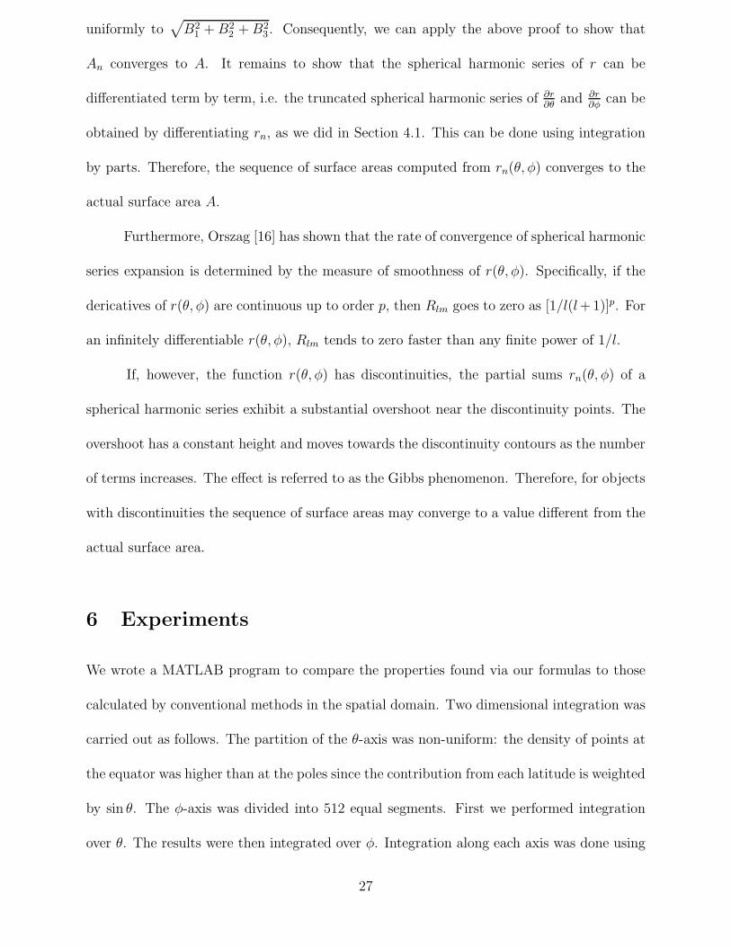
Figure 2: Mannequin head

Among the several objects tested was the mannequin head shown in Figure 2. Figures

3-4 present the moments of the mannequin head as a function of the maximum order l of

the coefficients retained in the expansion, in reference to the directly computed values. As

we can see from the graphs, the values of the moments converge rapidly: truncating the

spherical harmonic series at l = 8 was sufficient to achieve 99% accuracy.

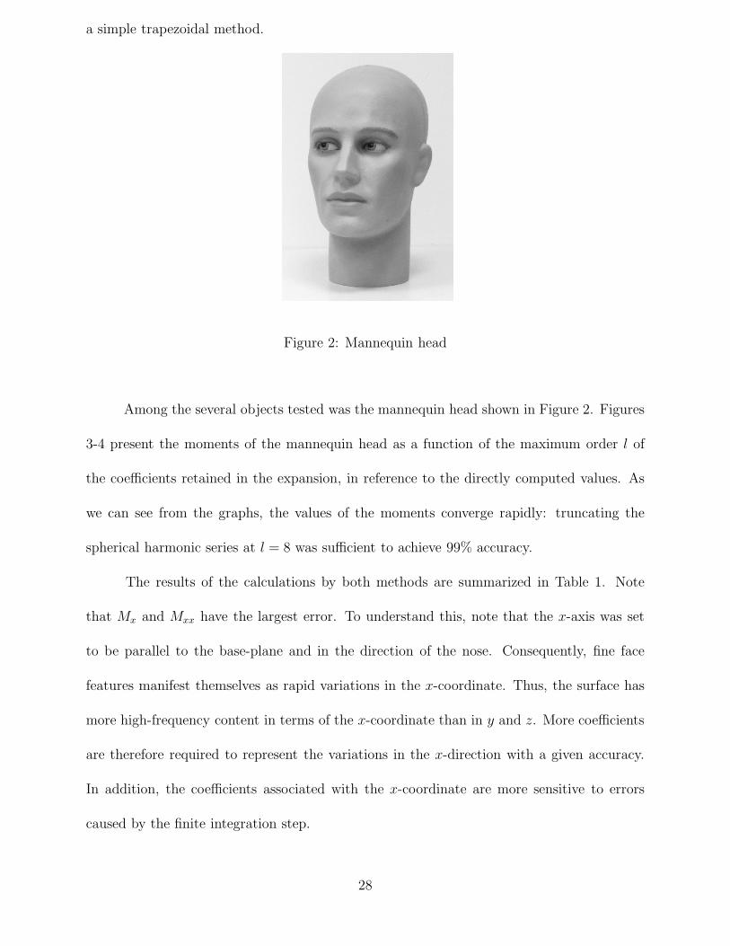
The results of the calculations by both methods are summarized in Table 1. Note

that Mx and Mxx have the largest error. To understand this, note that the x-axis was set

to be parallel to the base-plane and in the direction of the nose. Consequently, fine face

features manifest themselves as rapid variations in the x-coordinate. Thus, the surface has

more high-frequency content in terms of the x-coordinate than in y and z. More coefficients

are therefore required to represent the variations in the x-direction with a given accuracy.

In addition, the coefficients associated with the x-coordinate are more sensitive to errors

caused by the finite integration step.

28

0 2 4 6 83.4

3.45

3.5

3.55

3.6

3.65

l

Volume

0 2 4 6 8−0.1

−0.08

−0.06

−0.04

−0.02

0

l

Mx

(a) (b)

0 2 4 6 8−0.12

−0.1

−0.08

−0.06

−0.04

−0.02

0

l

My

0 2 4 6 80

0.02

0.04

0.06

0.08

0.1

0.12

l

Mz

(c) (d)

Figure 3: Volume and centroid of the head model as a function of l - the maximum orderof the coefficients retained in the expansion: (a) Volume; (b) Mx; (c) My; (d) Mz. Dashedline: direct computation; solid line: computation using spherical harmonic coefficients.

29

0 2 4 6 80.65

0.7

0.75

0.8

0.85

0.9

0.95

1

l

Mxx

0 2 4 6 80

0.02

0.04

0.06

0.08

0.1

l

Mxy

(a) (b)

0 2 4 6 8−0.25

−0.2

−0.15

−0.1

−0.05

0

l

Mxz

0 2 4 6 80.45

0.5

0.55

0.6

0.65

0.7

l

Myy

(c) (d)

0 2 4 6 8−0.06

−0.05

−0.04

−0.03

−0.02

−0.01

0

l

Myz

0 2 4 6 80.66

0.68

0.7

0.72

0.74

0.76

l

Mzz

(e) (f)

Figure 4: Second-order moments of the head model as a function of l - the maximum orderof the coefficients retained in the expansion: (a) Mxx; (b) Mxy; (c) Mxz; (d) Myy; (e) Myz ;(f) Mzz. Dashed line: direct computation; solid line: computation using spherical harmoniccoefficients.

30

Moment type Direct Calculation Spherical Harmonics for l = 8 Error (%)V 3.5977 3.5914 0.1747Mx -0.0945 -0.0958 1.3457My -0.0930 -0.0931 0.0828Mz 0.1174 0.1173 0.0770Mxx 0.9675 0.9594 0.8345Mxy 0.0930 0.0925 0.5843Mxz -0.2007 -0.2003 0.2343Myy 0.5073 0.5050 0.4533Myz -0.0557 -0.0554 0.5321Mzz 0.7575 0.7556 0.2403

Table 1: Volume, location of the centroid, and second order moments of the head model.

Referring to the surface area, a lower bound of 11.2 was obtained using the partition

Ωmn =

mπ

2≤ θ < (m + 1)

π

2, n

π

2≤ φ < (n + 1)

π

2

(0 ≤ m ≤ 1, 0 ≤ n ≤ 3 )

The upper bound was 14.2. The actual value of the surface area was 13.1, estimated by

discretization of (28):

A =∑

i

∑

j

|[~r(θi+1, φj) − ~r(θi, φj)] × [~r(θi, φj+1) − ~r(θi, φj)]|

We also tested our method on the near-Earth asteroid, 433 Eros. The NEAR-

Shoemaker Laser Rangefinder spacecraft [20] measured Eros’ surface height by firing a laser

pulse at Eros every second and recording how long it took the beam to reflect from the

surface. From these data scientists have built the first detailed maps and three-dimensional

model of an asteroid. The website accompanying Zuber et al. [20] provides both the spher-

ical harmonic coefficients of the asteroid, and its volume and moments obtained by direct

calculation. We computed the volume and moments of inertia via the spherical harmonic

coefficients, and compared them to the reference data provided. The asteroid was assumed

31

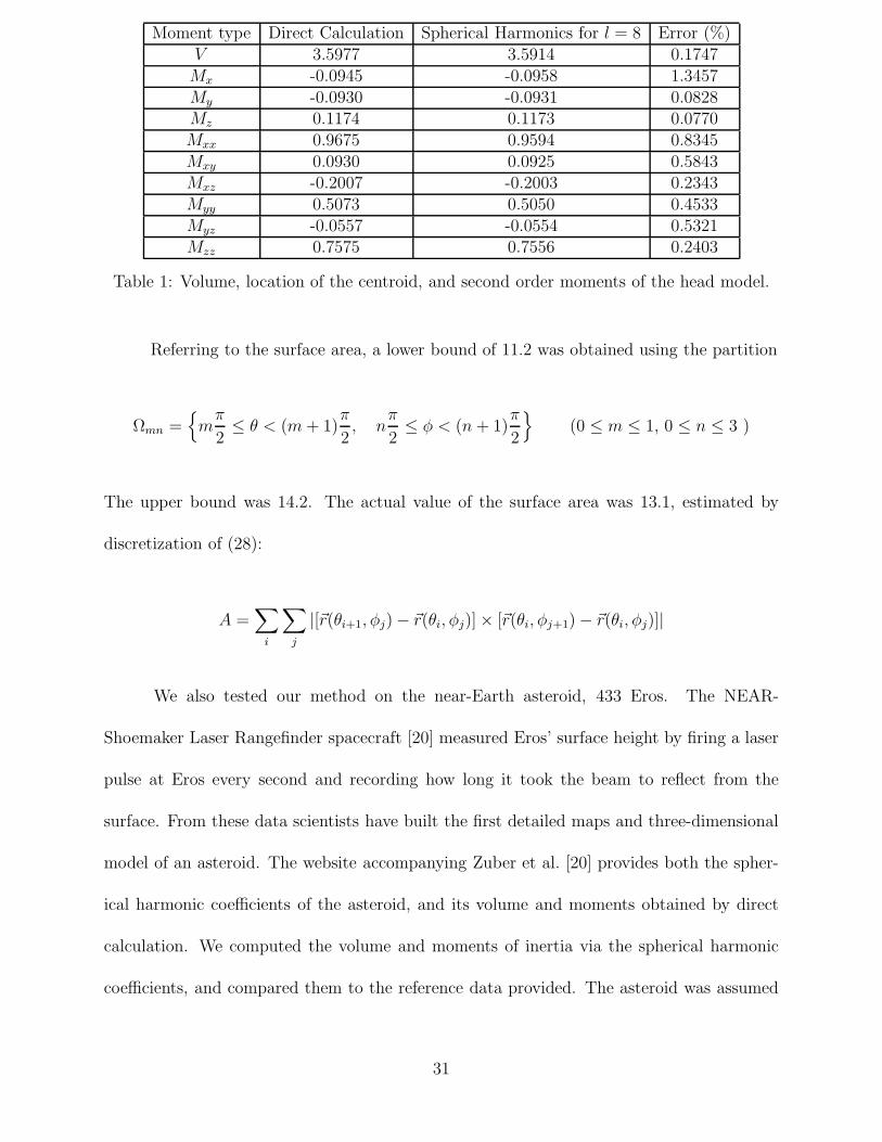
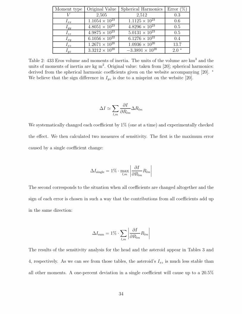
to have a uniform density of 2.67 g/cm3 [2]. As seen in Table 2, the correspondence between

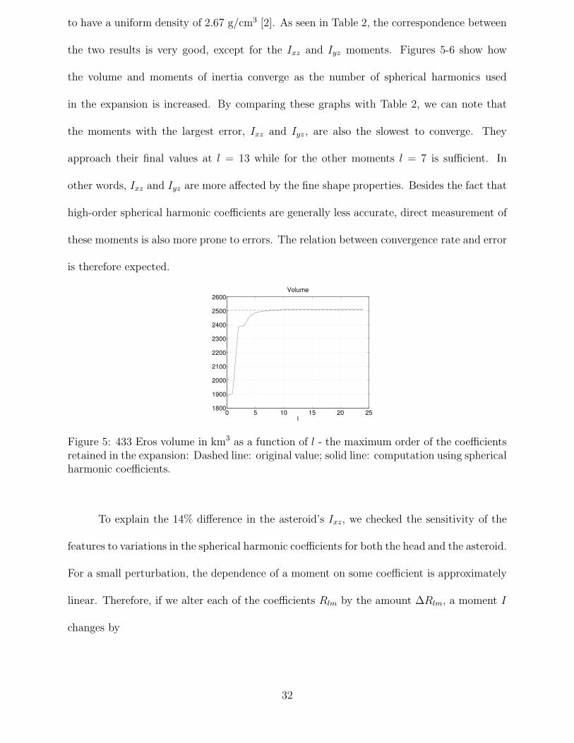
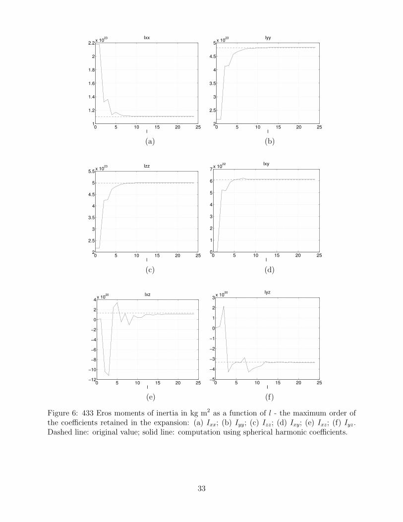
the two results is very good, except for the Ixz and Iyz moments. Figures 5-6 show how

the volume and moments of inertia converge as the number of spherical harmonics used

in the expansion is increased. By comparing these graphs with Table 2, we can note that

the moments with the largest error, Ixz and Iyz , are also the slowest to converge. They

approach their final values at l = 13 while for the other moments l = 7 is sufficient. In

other words, Ixz and Iyz are more affected by the fine shape properties. Besides the fact that

high-order spherical harmonic coefficients are generally less accurate, direct measurement of

these moments is also more prone to errors. The relation between convergence rate and error

is therefore expected.

0 5 10 15 20 251800

1900

2000

2100

2200

2300

2400

2500

2600

l

Volume

Figure 5: 433 Eros volume in km3 as a function of l - the maximum order of the coefficientsretained in the expansion: Dashed line: original value; solid line: computation using sphericalharmonic coefficients.

To explain the 14% difference in the asteroid’s Ixz, we checked the sensitivity of the

features to variations in the spherical harmonic coefficients for both the head and the asteroid.

For a small perturbation, the dependence of a moment on some coefficient is approximately

linear. Therefore, if we alter each of the coefficients Rlm by the amount ∆Rlm, a moment I

changes by

32

0 5 10 15 20 251

1.2

1.4

1.6

1.8

2

2.2x 10

23

l

Ixx

0 5 10 15 20 252

2.5

3

3.5

4

4.5

5x 10

23

l

Iyy

(a) (b)

0 5 10 15 20 252

2.5

3

3.5

4

4.5

5

5.5x 10

23

l

Izz

0 5 10 15 20 250

1

2

3

4

5

6

7x 10

22

l

Ixy

(c) (d)

0 5 10 15 20 25−12

−10

−8

−6

−4

−2

0

2

4x 10

20

l

Ixz

0 5 10 15 20 25−5

−4

−3

−2

−1

0

1

2

3x 10

20

l

Iyz

(e) (f)

Figure 6: 433 Eros moments of inertia in kg m2 as a function of l - the maximum order ofthe coefficients retained in the expansion: (a) Ixx; (b) Iyy; (c) Izz; (d) Ixy; (e) Ixz; (f) Iyz .Dashed line: original value; solid line: computation using spherical harmonic coefficients.

33

Moment type Original Value Spherical Harmonics Error (%)V 2,505 2,512 0.3Ixx 1.1054 × 1023 1.1125 × 1023 0.6Iyy 4.8051 × 1023 4.8296 × 1023 0.5Izz 4.9875 × 1023 5.0131 × 1023 0.5Ixy 6.1056 × 1022 6.1276 × 1022 0.4Ixz 1.2671 × 1020 1.0936 × 1020 13.7Iyz 3.3212 × 1020 −3.3891 × 1020 2.0 ∗

Table 2: 433 Eros volume and moments of inertia. The units of the volume are km3 and theunits of moments of inertia are kg m2. Original value: taken from [20]; spherical harmonics:derived from the spherical harmonic coefficients given on the website accompanying [20]. ∗

We believe that the sign difference in Iyz is due to a misprint on the website [20].

∆I '∑

l,m

∂I

∂Rlm

∆Rlm

We systematically changed each coefficient by 1% (one at a time) and experimentally checked

the effect. We then calculated two measures of sensitivity. The first is the maximum error

caused by a single coefficient change:

∆Isingle = 1% · maxl,m

∣

∣

∣

∣

∂I

∂Rlm

Rlm

∣

∣

∣

∣

The second corresponds to the situation when all coefficients are changed altogether and the

sign of each error is chosen in such a way that the contributions from all coefficients add up

in the same direction:

∆Isum = 1% ·∑

l,m

∣

∣

∣

∣

∂I

∂Rlm

Rlm

∣

∣

∣

∣

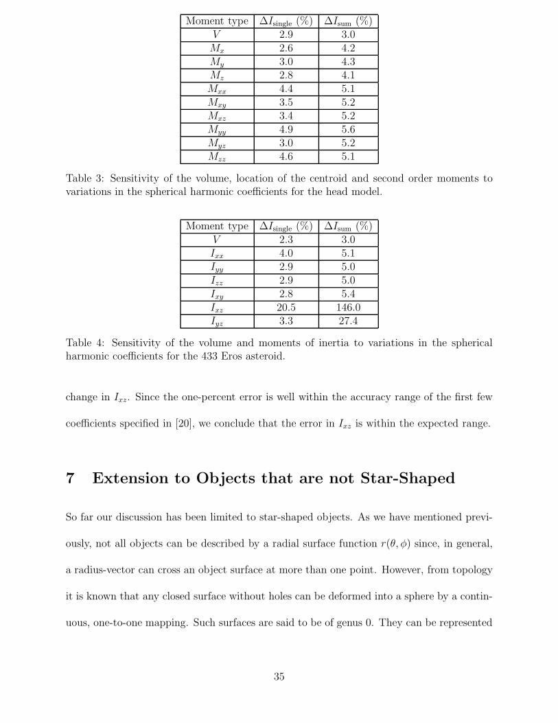
The results of the sensitivity analysis for the head and the asteroid appear in Tables 3 and

4, respectively. As we can see from those tables, the asteroid’s Ixz is much less stable than

all other moments. A one-percent deviation in a single coefficient will cause up to a 20.5%

34

Moment type ∆Isingle (%) ∆Isum (%)V 2.9 3.0Mx 2.6 4.2My 3.0 4.3Mz 2.8 4.1Mxx 4.4 5.1Mxy 3.5 5.2Mxz 3.4 5.2Myy 4.9 5.6Myz 3.0 5.2Mzz 4.6 5.1

Table 3: Sensitivity of the volume, location of the centroid and second order moments tovariations in the spherical harmonic coefficients for the head model.

Moment type ∆Isingle (%) ∆Isum (%)V 2.3 3.0Ixx 4.0 5.1Iyy 2.9 5.0Izz 2.9 5.0Ixy 2.8 5.4Ixz 20.5 146.0Iyz 3.3 27.4

Table 4: Sensitivity of the volume and moments of inertia to variations in the sphericalharmonic coefficients for the 433 Eros asteroid.

change in Ixz. Since the one-percent error is well within the accuracy range of the first few

coefficients specified in [20], we conclude that the error in Ixz is within the expected range.

7 Extension to Objects that are not Star-Shaped

So far our discussion has been limited to star-shaped objects. As we have mentioned previ-

ously, not all objects can be described by a radial surface function r(θ, φ) since, in general,

a radius-vector can cross an object surface at more than one point. However, from topology

it is known that any closed surface without holes can be deformed into a sphere by a contin-

uous, one-to-one mapping. Such surfaces are said to be of genus 0. They can be represented

35

in a parametric form as

~r(θ, φ) = x(θ, φ)x + y(θ, φ)y + z(θ, φ)z (62)

where 0 ≤ θ ≤ π, 0 ≤ φ ≤ 2π. It should be emphasized that θ and φ here are not

necessarily the latitude and the azimuth of the boundary point. When an object surface

is given as a collection of points (xi, yi, zi), we need to assign spherical coordinates (θi, φi)

to each point. Spherical parameterization is usually formulated as an optimization problem

that minimizes some measure of the distortion of the surface net in the mapping. In [1] the

objective functional to be maximized is the sum of cosines of four sides over all faces on

the sphere corresponding to elementary squares on the original surface. There are also two

additional constraints: (i) any object surface region must map to a region of proportional

area on the sphere, and (ii) no angle of any spherical quadrilateral must become negative or

exceed π. The algorithm that was originally developed in [4] and later extended and applied

to surface analysis in [7] uses a functional quantifying the discrepancy between geodesic

distances between a set of points on the surface and the corresponding distances on the

sphere.

Once we have the spherical parameterization (62), we can expand x(θ, φ), y(θ, φ), and

z(θ, φ) in a series of spherical harmonics. Let Xlm, Ylm, and Zlm denote the respective

sets of spherical harmonic coefficients. In this section we shall show that the moments and

bounds on the surface area can be extracted directly from Xlm, Ylm, and Zlm.

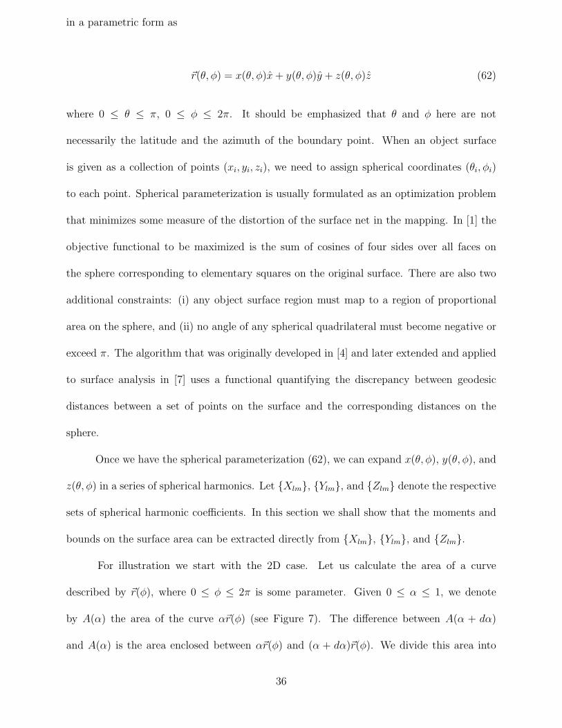
For illustration we start with the 2D case. Let us calculate the area of a curve

described by ~r(φ), where 0 ≤ φ ≤ 2π is some parameter. Given 0 ≤ α ≤ 1, we denote

by A(α) the area of the curve α~r(φ) (see Figure 7). The difference between A(α + dα)

and A(α) is the area enclosed between α~r(φ) and (α + dα)~r(φ). We divide this area into

36

Figure 7: Illustration of Area Calculation for a 2D Non-Star-Shaped Object

infinitesimal parallelograms, each one defined by points α~r(φ), α~r(φ + dφ), (α + dα)~r(φ),

and (α + dα)~r(φ + dφ). The contribution of such a parallelogram to the total area can be

expressed as a vector product

d~a = dα~r × αd~r

dφdφ

It can be either positive or negative. For example, at φ = φ1 the point enters the region

as α is increased. The angle from dα~r(φ1) to α d~rdφ

(φ1)dφ1 is less than 180o, so d~a points in

the positive z-direction. On the other hand, at φ = φ2 the point leaves the region as α is

increased. The angle from dα~r(φ2) to α d~rdφ

(φ2)dφ2 is greater than 180o, so d~a points in the

negative z-direction. It follows that the area of the curve is given by

37

A =

∣

∣

∣

∣

∫ 1

α=0

∫ 2π

φ=0

dα~r × αd~r

dφdφ

∣

∣

∣

∣

=1

2

∣

∣

∣

∣

∫ 2π

φ=0

~r × d~r

dφdφ

∣

∣

∣

∣

Now we return to the 3D case. To calculate the moments of a figure given by (62),

let us imagine that the object surface is inflated from the origin to its final size in such a

way that the intermediate surface S(α) is described by α~r(θ, φ), 0 ≤ α ≤ 1. Next divide the

region of space enclosed between S(α) and S(α + dα) into infinitesimal parallelepipeds with

edges determined by α∂~r∂θ

dθ, α ∂~r∂φ

dφ, and dα~r. The volume of such a parallelepiped can be

written as a triple scalar product

dv =

(

α∂~r

∂θdθ × α

∂~r

∂φdφ

)

· dα~r

Note that dv can be both positive and negative. This can be understood as follows. If some

radius vector crosses the object surface several times, the points on it are also taken into

account more than once. As the object surface is inflated, each time a point enters the object

it is taken with a positive sign, and each time a point comes out of the object, it is taken

with a negative sign. The points inside the surface are counted an odd number of times, for

a net count of 1, whereas the points outside of the surface are counted an even number of

times, for a net count of 0. Therefore, the moments of the figure are given by

Mijk =

∫

Object

xiyjzkdv

=

∫ 1

α=0

∫ π

θ=0

∫ 2π

φ=0

(αx)i(αy)j(αz)k

(

α∂~r

∂θdθ × α

∂~r

∂φdφ

)

· dα~r

38

=1

i + j + k + 3

∫ π

θ=0

∫ 2π

φ=0

xiyjzk

(

∂~r

∂θ× ∂~r

∂φ

)

· ~rdθdφ (63)

Expressing the triple scalar product as a determinant yields

Mijk =1

i + j + k + 3

∫ π

θ=0

∫ 2π

φ=0

xiyjzk

∣

∣

∣

∣

∣

∣

∣

∣

∣

∣

∣

∣

x y z

xθ yθ zθ

xφ yφ zφ

∣

∣

∣

∣

∣

∣

∣

∣

∣

∣

∣

∣

dθdφ (64)

To validate the above formula, we took as an example a sphere of a unit radius whose center

is shifted from the origin to the point (x0, y0, z0). The parameterization is then very simple:

x(θ, φ) = x0 + sin θ cos φ

y(θ, φ) = y0 + sin θ sin φ

z(θ, φ) = z0 + cos θ

It is easy to see that substituting this into (64) with i = j = k = 0 gives the volume of 4π/3,

as expected. It can also be shown that if θ and φ are the latitude and the azimuth of the

boundary point, then (64) reduces to the well-known formula for star-shaped regions.

Now let us denote the integrand in eq. (64) by F (θ, φ). Assuming that we know its

spherical harmonic coefficients, Flm, we can write the moments of an object in the form

Mijk =1

i + j + k + 3

∫ π

θ=0

∫ 2π

φ=0

[

∞∑

l=0

l∑

m=−l

FlmYlm(θ, φ)

]

dθdφ

39

Using the definition in (50) and taking into account that Ilm(Ω) 6= 0 only for m = 0, we

obtain

Mijk =1

i + j + k + 3

∞∑

l=0

Fl,0Il,0(Ω) (65)

To calculate Fl,0 recall that in Section 4.1 we saw how the spherical harmonic coefficients

of rθ sin θ and rφ can be obtained from those of r by means of a 3D convolution. Using the

same technique, we can express the spherical harmonic coefficients of G(θ, φ) = F (θ, φ) sin θ

in terms of Xlm, Ylm, and Zlm. We shall denote them by Glm. The spherical

harmonic coefficients of h(θ, φ) = 1sin θ

can be written according to (4) as

Hlm =

∫ π

θ=0

∫ 2π

φ=0

Y ∗lm(θ, φ)dθdφ

It can be seen that Hlm 6= 0 only for m = 0. Finally, applying the 3D convolution theorem

(7) to F (θ, φ) = G(θ,φ)sin θ

yields

Fl,0 =

∞∑

l1=0

∞∑

l2=0

Gl1,0H∗l2,0

√

(2l1 + 1)(2l2 + 1)

4π(2l + 1)〈l1, l2; 0, 0|l, 0〉2 (66)

We have thus shown that the moments of a figure can be calculated directly from the spherical

harmonic descriptors. In the example of a shifted sphere we saw before,

G(θ, φ) = sin2 θ =4

3

√πY0,0(θ, φ) − 4

3

√

π

5Y2,0(θ, φ)

In an experiment, we substituted these coefficients into (66) using 50 terms in the expansion

of 1sin θ

to obtain Fl,0. Then from (65) we obtained the volume of the unit sphere with

error less than 0.1%. As for the surface area, formula (28) is valid for any parameterization

40

of the form (62), and the rest of the calculations are similar to the above.

However, the numerical stability of this method could be somewhat problematic. Since

G(θ, φ) is divided by sin θ to get F (θ, φ), it follows that G(θ, φ) tends to zero at least as

sin θ when θ approaches 0 or π. But if a small error is introduced in the spherical harmonic

coefficients Glm, it can be potentially amplified by eq. (66). Therefore we conclude that

the star-shaped representation is advantageous, for it is both computationally simpler and

more accurate.

8 Complexity Analysis and Transform Method

As one can appreciate, the numerical complexity of our method is determined by the number

of operations that need to be performed for calculating spherical harmonic coefficients of

a product of two functions. It is apparent from (7) that if Alm = 0 and Blm = 0 for

l > N , the total number of operations involved in calculating Clm for each pair l, m scales

as N3. Furthermore, for a Clebsch-Gordan coefficient 〈l1, l2; m1, m2|l, m〉 to be non-zero it

is necessary that l ≤ l1 + l2. Consequently, Clm = 0 for l ≥ 2N − 1, i.e. the number

of coefficients to be calculated is O(N2). It follows that O(N5) arithmetic operations are

required to evaluate (7) for all retained l, m. In addition, O(N5) Clebsch-Gordan coefficients

must be calculated off-line and stored somewhere in computer memory. In applications

for which the amount of memory required becomes prohibitively large, the Clebsch-Gordan

coefficients have to be calculated on the fly. They are usually expressed in terms of the

Wigner 3j-symbols [19]. It can then be shown that one Clebsch-Gordan coefficient can be

calculated in a linear time. It follows that, in this case, the total computational complexity of

(7) for all retained l, m is O(N6). Our experience shows that spherical harmonic coefficients

up to order l = 15 are sufficient to represent a typical 3D object with reasonable accuracy.

41

In this range our method could be substantially faster than the reconstruction of the original

object. However, for large N the direct evaluation of (7) is in a too unfavorable competition

position with the spatial domain method.

Fortunately, it is possible to evaluate eq. (7) indirectly, by a transform method that

does not require knowing the Clebsch-Gordan coefficients [15]. This transform method is

based on the fact that if a function h(θ, φ) is strictly bandlimited such that Clm = 0 for l ≥ b,

then to obtain its spherical harmonic coefficients one does not necessarily have to perform

the integral in eq. (4). Instead, it is sufficient to sample h(θ, φ) at the equiangular grid of

points (θj , φk), j = 0, . . . , 2b − 1, k = 0, . . . , 2b − 1, where θj = πj/2b and φk = πk/b. It

is shown in [5] that h can be recovered from these samples and, furthermore, the spherical

harmonic coefficients can be computed in terms of them by the discrete spherical harmonic

transform (SHT):

Clm =

√2π

2b

2b−1∑

j=0

2b−1∑

k=0

a(b)j h(θj , φk)Y

∗lm(θj , φk)

for l < b and |m| ≤ l. The weights a(b)j are determined by solving a system of 2b linear

equations in 2b unknowns. The SHT is calculated using separation of variables. One needs

to perform 2b discrete Fourier transforms (DFT) and 2b discrete Legendre transforms (DLT),

each one of length 2b. The DFT is usually implemented by the fast Fourier transform

algorithm whose complexity is O(b log b). The straightforward evaluation of the DLT has

the complexity of O(b2). With the invention of the fast SHT [5], the complexity of the DLT

has been reduced to O(b log2 b). Therefore, the SHT can be computed in O(b2 log2 b) time.

In a later work [9], an algorithm for the inverse SHT was developed which has the same

complexity. Now we can calculate Clm from eq. (7) with a three-step procedure, just like

in the case of a one-dimensional convolution:

42

(i) reconstruct the values of f from Alm and g from Blm at (2(2N − 1))2 equiangularly

distributed points using the inverse SHT;

(ii) multiply f by g to get the values of h at these points which requires O(N2) operations;

(iii) compute Clm from these samples by the SHT.

As we see, the complexity of our method can be made equal to that of the SHT, i.e.

O(N2 log2 N).

Since steps (i) and (iii) in the transform method are the inverse of each other, we could

optimize our method so that some of the intermediate computations would be saved. For

example, to obtain the x-coordinate of the centroid in Section 3, we calculate Slm from

Rlm and then Qlm from Slm, according to (13-14). If the transform method is used,

we perform the SHT on s(θ, φ) to get Slm followed immediately by the inverse SHT on

Slm. It is clearly possible to skip these two operations. Moreover, we can first compute the

maximum order of the spherical harmonic coefficients in the expansion of the integrand on

the right-hand side of (18). Then we reconstruct r(θ, φ) at a sufficient number of points and

evaluate the integrand at those points. The value of x is proportional to the DC coefficient

of the integrand. In this way, the calculations are reduced to one SHT and one inverse SHT.

9 Conclusions and Future Work

The representation of star-shaped objects by the spherical harmonic coefficients of their

boundary function is used in a variety of scientific domains. In this paper, we explicitly

expressed the volume, centroid, second order moments and bounds on the surface area in

terms of the spherical harmonic coefficients, without an intermediate reconstruction step.

We proved the convergence of the geometric properties, suggested an efficient computational

scheme and outlined an extension to genus-0 objects that are not star-shaped. Experiments

43

with real objects, for which the true values of the geometric properties can be estimated,

support the theoretical results.

One direction for further work is motivated by the fact that even with the fast SHT,

the complexity of the spherical harmonic method is higher than that of the 2D FFT -

O(N2 log N). Orszag [16] proposed an alternative expansion for problems in spherical ge-

ometry based on special Fourier series. The advantage of the new Fourier series on spheres

is that the SHT is replaced there by the regular FFT, so they are computationally simpler.

Our preliminary results show that this basis is not inferior to spherical harmonics as far as

the efficiency of representing 3D objects is concerned. Future work may also address in more

depth the numerical issues of the method for non-star-shaped objects.

APPENDIX

In the Appendix, we shall obtain the expressions for the second-order moments. Proceeding

similarly to Section 3.4, we have for the xy-moment

Mxy =

∫

Object

xydv =

∫ r(θ,φ)

ρ=0

∫ π

θ=0

∫ 2π

φ=0

(ρ sin θ cos φ)(ρ sin θ sin φ)ρ2 sin θdρdθdφ

=1

5

∫ π

θ=0

∫ 2π

φ=0

r5(θ, φ)(sin θ cos φ)(sin θ sin φ) sin θdθdφ

Now we can expand (sin θ cos φ)(sin θ sin φ) in a series of spherical harmonics using the 3D

convolution theorem (8) with f(θ, φ) = sin θ cos φ and g(θ, φ) = sin θ sin φ. Taking into

account (21) and (23), we obtain

(sin θ cos φ)(sin θ sin φ) = C(xy)2,−2Y2,−2(θ, φ) + C

(xy)2,2 Y2,2(θ, φ)

44

with the coefficients of the expansion given by

C(xy)2,−2 = i

√

π

5〈1, 1; 0, 0|2, 0〉 〈1, 1;−1,−1|2,−2〉

C(xy)2,2 = −i

√

π

5〈1, 1; 0, 0|2, 0〉 〈1, 1; 1, 1|2, 2〉

Then according to the Parseval theorem (9)

Mxy =1

5

(

C(xy)∗2,−2 P2,−2 + C

(xy)∗2,2 P2,2

)

(67)

As we can see from the last equation, in order to calculate the xy-moment it is sufficient to

know the spherical harmonic coefficients of r5(θ, φ) corresponding to (l, m) = (2,−2) and

(2, 2). The xz-moment can be written in the form

Mxz =

∫

Object

xzdv =

∫ r(θ,φ)

ρ=0

∫ π

θ=0

∫ 2π

φ=0

(ρ sin θ cos φ)(ρ cos θ)ρ2 sin θdρdθdφ

=1

5

∫ π

θ=0

∫ 2π

φ=0

r5(θ, φ)(sin θ cos φ)(cos θ) sin θdθdφ

Using (8), (21), and (25), we can write (sin θ cos φ)(cos θ) as a linear combination of spherical

harmonics:

(sin θ cos φ)(cos θ) = C(xz)2,−1Y2,−1(θ, φ) + C

(xz)2,1 Y2,1(θ, φ)

where

45

C(xz)2,−1 =

√

2π

5〈1, 1; 0, 0|2, 0〉 〈1, 1;−1, 0|2,−1〉

C(xz)2,1 = −

√

2π

5〈1, 1; 0, 0|2, 0〉 〈1, 1; 1, 0|2, 1〉

Now we apply (9) to get

Mxz =1

5

(

C(xz)2,−1P2,−1 + C

(xz)2,1 P2,1

)

(68)

In a similar way, the yy-moment is given by

Myy =

∫

Object

y2dv =

∫ r(θ,φ)

ρ=0

∫ π

θ=0

∫ 2π

φ=0

(ρ sin θ sin φ)2ρ2 sin θdρdθdφ

=1

5

∫ π

θ=0

∫ 2π

φ=0

r5(θ, φ)(sin θ sin φ)2 sin θdθdφ

Using (8) and (23), we obtain:

(sin θ sin φ)2 = C(yy)0,0 Y0,0(θ, φ) + C

(yy)2,−2Y2,−2(θ, φ) + C

(yy)2,0 Y2,0(θ, φ) + C

(yy)2,2 Y2,2(θ, φ)

where the coefficients of the expansion are given by

C(yy)0,0 = −2

√π 〈1, 1; 0, 0|0, 0〉 〈1, 1; 1,−1|0, 0〉

C(yy)2,−2 = −

√

π

5〈1, 1; 0, 0|2, 0〉 〈1, 1;−1,−1|2,−2〉

46

C(yy)2,0 = −2

√

π

5〈1, 1; 0, 0|2, 0〉 〈1, 1; 1,−1|2, 0〉

C(yy)2,2 = −

√

π

5〈1, 1; 0, 0|2, 0〉 〈1, 1; 1, 1|2, 2〉

Then, according to the Parseval theorem, we get the following expression for the yy-moment:

Myy =1

5

(

C(yy)0,0 P0,0 + C

(yy)2,−2P2,−2 + C

(yy)2,0 P2,0 + C

(yy)2,2 P2,2

)

(69)

Next, the yz-moment can be written in the form

Myz =

∫

Object

yzdv =

∫ r(θ,φ)

ρ=0

∫ π

θ=0

∫ 2π

φ=0

(ρ sin θ sin φ)(ρ cos θ)ρ2 sin θdρdθdφ

=1

5

∫ π

θ=0

∫ 2π

φ=0

r5(θ, φ)(sin θ sin φ)(cos θ) sin θdθdφ

According to (8), (23), and (25)

(sin θ sin φ)(cos θ) = C(yz)2,−1Y2,−1(θ, φ) + C

(yz)2,1 Y2,1(θ, φ)

where

C(yz)2,−1 = i

√

2π

5〈1, 1; 0, 0|2, 0〉 〈1, 1;−1, 0|2,−1〉

C(yz)2,1 = i

√

2π

5〈1, 1; 0, 0|2, 0〉 〈1, 1; 1, 0|2, 1〉

We have from (9)

47

Myz =1

5

(

C(yz)∗2,−1 P2,−1 + C

(yz)∗2,1 P2,1

)

(70)

Finally, the zz-moment is given by

Mzz =

∫

Object

z2dv =

∫ r(θ,φ)

ρ=0

∫ π

θ=0

∫ 2π

φ=0

(ρ cos θ)2ρ2 sin θdρdθdφ

=1

5

∫ π

θ=0

∫ 2π

φ=0

r5(θ, φ) cos2 θ sin θdθdφ

Using (8) and (25), we get

cos2 θ = C(zz)0,0 Y0,0(θ, φ)C

(zz)2,0 Y2,0(θ, φ)

where

C(zz)0,0 = 2

√π 〈1, 1; 0, 0|0, 0〉2

C(zz)2,0 = 2

√

π

5〈1, 1; 0, 0|2, 0〉2

Finally, according to (9)

Mzz =1

5

(

C(zz)0,0 P0,0 + C

(zz)2,0 P2,0

)

(71)

48

References

[1] Ch. Brechbuhler, G. Gerig, and O. Kubler, Parametrization of Closed Surfaces for 3-D

Shape Description, Computer Vision and Image Understanding, Vol. 61, No. 2, March,

pp.154-170, 1995.

[2] D. T. Britt, D. Yeomans, and G. J. Consolmagno, The porosity of 433 Eros, 32nd Lunar

and Planetary Science Conference, March 12-16, 2001, Houston, Texas. Available on-

line at [http://www.lpi.usra.edu/meetings/lpsc2001/pdf/1212.pdf].

[3] C. Cohen-Tannoudji, B. Diu, and F. Lalo, Quantum Mechanics, John Wiley & Sons,

1977.

[4] T.F. Cox and M.A.A. Cox, Multidimensional scaling on a sphere, Communications in

Statistics: Theory and Methods, pp. 2943-2953, Vol. 20, 1991.

[5] J.R. Driscoll and D.M. Healy, Jr., Computing Fourier Transforms and Convolutions on

the 2-Sphere, Advances in Applied Mathematics 15, pp. 202-250 (1994).

[6] B.S. Duncan, A.J. Olson, Approximation and characterization of molecular surfaces,

Biopolymers 33 (1993), pp. 219-229.

[7] A. Elad and R. Kimmel, Spherical flattening of the cortex surface, in R. Malladi (ed.),

Geometric Methods in Biomedical Image Processing, Springer, 2002.

[8] E.J. Garboczi, Three-dimensional mathematical analysis of particle shape using X-ray

tomography and spherical harmonics: application to aggregates used in concrete, Ce-

ment and Concrete Research 32 (2002), pp. 1621-1638.

[9] D. Healy Jr., D. Rockmore, P. Kostelec, and S. Moore, FFTs for the 2-Sphere - Improve-

ments and Variations, The Journal of Fourier Analysis and Applications, 9:4 (2003),

49

pp. 341 - 385. Available on-line at: [http://www.cs.dartmouth.edu/∼geelong/sphere/s2-

main.pdf].

[10] W. Kaula, Theory of Satellite Geodesy, Dover, New York, 1960; Geodesy for the Layman,

Defense Mapping Agency Technical Report, 1983. Available at http://geodesy.eng.ohio-

state.edu/course/refpapers/NIMA.pdf.

[11] M. Kazhdan, T. Funkhouser and S. Rusinkiewicz, “Rotation invariant spherical har-

monic representation of 3D shape descriptors”, Proc. Eurographics Symposium on Ge-

ometry Processing, pp. 156-165, 2003.

[12] Kellogg, Oliver Dimon, Foundations of Potential Theory, New York: Ungar, 1970.

[13] N. Kiryati and D. Maydan, Calculating Geometric Properties from Fourier Representa-

tion, Pattern Recognition, Vol. 22, No. 5, pp. 469-475, 1989.

[14] R. Liboff, Introductory Quantum Mechanics (3rd Edition), Addison Wesley, 1998.

[15] S.A. Orszag, Transform Method for the Calculation of Vector-Coupled Sums: Appli-

cation to the Spectral Form of the Vorticity Equation, Journal of the Atmospheric

Sciences, Volume 27, pp. 890-895 (1970).

[16] S.A. Orszag, Fourier Series on Spheres, Monthly Weather Review, Vol. 102, No. 1, pp.

56-75, January 1974.

[17] D. Saupe and D.V. Vranic, 3D model retrieval with spherical harmonics and moments,

Proceedings Mustererkennung 2001 (DAGM 2001), Munich, Sept. 2001. Available on-

line at [http://www.inf.uni-konstanz.de/cgip/bib/files/SaVr01.pdf].

50

[18] R.B. Schudy and D.H. Ballard, “Towards an anatomical model of heart motion as seen

in 4-D cardiac ultrasound data”, Proc. 6th Conf. on Computer Applications in Radiology

and Computer-Aided Analysis of Radiological Images, 1979.

[19] Eric W. Weisstein, ”Clebsch-Gordan Coefficient”, From MathWorld–A Wolfram Web

Resource. http://mathworld.wolfram.com/Clebsch-GordanCoefficient.html

[20] Zuber, M.T., D.E. Smith, A.F. Cheng, J.B. Garvin, O. Aharonson, T.D. Cole, P.J.

Dunn, Y. Guo, F.G. Lemoine, G.A. Neumann, D.D. Rowlands, and M.H. Torrence,

The Shape of 433 Eros from the NEAR-Shoemaker Laser Rangefinder, Science, 289,

1788-1793, 2000. (Additional material for this paper is available at http://www-

geodyn.mit.edu/near/nlr.30day.html.)

51