Progress In Electromagnetics Research, PIER 83, 55–80, 2008 CALCULATING THE RADAR CROSS SECTION OF THE RESISTIVE TARGETS USING THE HAAR WAVELETS S. Hatamzadeh-Varmazyar Department of Electrical Engineering Islamic Azad University Science and Research Branch, Tehran, Iran M. Naser-Moghadasi Central Commission for Scientific Literacy & Art Societies Islamic Azad University Science and Research Branch, Tehran, Iran E. Babolian Department of Mathematics Tarbiat Moallem University 599 Taleghani Avenue, Tehran 15618, Iran Z. Masouri Department of Mathematics Islamic Azad University Science and Research Branch, Tehran, Iran Abstract—In this paper, the Haar wavelets basis functions are applied to the method of moments to calculate the radar cross section of the resistive targets. This problem is modeled by the integral equations of the second kind. An effective numerical method for solving these integral equations is proposed. The problem is treated in detail, and illustrative computations are given for several cases. This method can be generalized to apply to objects of arbitrary geometry.
Transcript
Progress In Electromagnetics Research, PIER 83, 55–80, 2008
CALCULATING THE RADAR CROSS SECTION OF THERESISTIVE TARGETS USING THE HAAR WAVELETS
S. Hatamzadeh-Varmazyar
Department of Electrical EngineeringIslamic Azad UniversityScience and Research Branch, Tehran, Iran
M. Naser-Moghadasi
Central Commission for ScientificLiteracy & Art SocietiesIslamic Azad UniversityScience and Research Branch, Tehran, Iran
E. Babolian
Department of MathematicsTarbiat Moallem University599 Taleghani Avenue, Tehran 15618, Iran
Z. Masouri
Department of MathematicsIslamic Azad UniversityScience and Research Branch, Tehran, Iran
Abstract—In this paper, the Haar wavelets basis functions are appliedto the method of moments to calculate the radar cross section of theresistive targets. This problem is modeled by the integral equationsof the second kind. An effective numerical method for solving theseintegral equations is proposed. The problem is treated in detail, andillustrative computations are given for several cases. This method canbe generalized to apply to objects of arbitrary geometry.
56 Hatamzadeh-Varmazyar et al.
1. INTRODUCTION
The development of numerical methods for solving integral equationsin Electromagnetics has attracted intensive researches for more thanfour decades [1, 2]. The use of high-speed computers allows one tomake more computations than ever before. During these years, carefulanalysis has paved the way for the development of efficient and effectivenumerical methods and, of equal importance, has provided a solidfoundation for a through understanding of the techniques.
Over several decades, electromagnetic scattering problems havebeen the subject of extensive researches (see [3–54]). Scattering fromarbitrary surfaces such as square, cylindrical, circular, spherical [3–9]are commonly used as test cases in computational Electromagnetics,because analytical solutions for scattered fields can be derived for thesegeometries [3].
An important parameter in scattering studies is the electromag-netic scattering by a target which is usually represented by its echoarea or radar cross section (RCS) [55]. The echo area or RCS is de-fined as the area intercepting the amount of power that, when scatteredisotropically, produces at the receiver a density that is equal to the den-sity scattered by the actual target [56]. For a two-dimensional targetthe scattering parameter is referred to as the scattering width (SW) oralternatively as the radar cross section per unit length.
When the transmitter and receiver are at the same location, theRCS is usually referred to as monostatic (or backscattered) and it isreferred to as bistatic when the two are at different locations [55].Observations made toward directions that satisfy Snell’s law ofreflection are usually referred to as specular. Therefore the RCS oftarget is very important parameter which characterizes its scatteringproperties. A plot of the RCS as a function of the space coordinates isusually referred to as the RCS pattern.
Calculating the radar cross section of the resistive targets leads tosolve the integral equations of the second kind with complex kernels.Of course, if the resistance of the target approaches to zero, then theproblem is modeled by integral equations of the first kind. However,for solving integral equations of the second kind, several numericalapproaches have been proposed. These numerical methods often usethe basis functions and transform the integral equation to a linearsystem that can be solved by direct or iterative methods [57]. Itis important in these methods to select an appropriate set of basisfunctions so that the approximate solution of integral equation has agood accuracy.
It is the purpose of this paper to use the Haar wavelets as a set
Progress In Electromagnetics Research, PIER 83, 2008 57
of orthogonal basis functions and to apply them to the method ofmoments for calculating the radar cross section of the resistive targets.Using this method, the second kind integral equation reduces to alinear system of algebraic equations. Solving this system gives anapproximate solution for these problems.
First of all, an extensive review of wavelets containing thedefinition, expansion and properties is performed. After this, theelectric field integral equation is introduced. Then, the method ofmoments is proposed for solving integral equations of the second kindusing Haar wavelets basis functions. Finally, the problem of calculatingthe radar cross section of the resistive strips is described in detailand solved by the presented method, and illustrative computationsare given for several cases.
2. WAVELET: DEFINITION, EXPANSION, ANDPROPERTIES
A wavelet is a “small wave”, which has its energy concentrated intime to give a tool for the analysis of transient, nonstationary, ortime-varying phenomena [58]. It still has the oscillating wave-likecharacteristic but also has the ability to allow simultaneous time andfrequency analysis with a flexible mathematical function.
In this section, the definition of wavelets and expansion of anyfunction f(t) in terms of these basis functions is presented. Also, someproperties of wavelets are surveyed.
2.1. Definition and Expansion
We start by defining the scaling function and then define the waveletin terms of it.
Let L2(R) be the space of square integrable functions. A set ofscaling functions in terms of integer translates of the basic scalingfunction or father wavelet ϕ(t) is defined by [58]
ϕk(t) = ϕ(t − k), k ∈ Z, ϕ ∈ L2(R). (1)
The subspace of L2(R) spanned by these functions is defined as
V0 = Spank∈Z
ϕk(t). (2)
This means that
f(t) =∑
k
ckϕk(t) for any f(t) ∈ V0. (3)
58 Hatamzadeh-Varmazyar et al.
One can generally increase the size of the subspace spanned bychanging the time scale of the scaling function. A two-dimensionalfamily of functions is generated from the basic scaling function or fatherwavelet by scaling and translation by [58]
ϕj, k(t) = 2j/2ϕ(2jt − k
), (4)
whose span over k is
Vj = Spank∈Z
ϕk (2jt) = Spank∈Z
ϕj, k(t). (5)
So, ϕj, k(t)k is a basis for Vj . This means that if f(t) ∈ Vj , then itcan be expressed as
f(t) =∑k∈Z
ckϕj, k(t), (6)
where Eq. (6) represents the projection of the function f onto thesubspace of scaling functions or father wavelets at resolution j.
According to the above definitions, it is clear that
Vj ⊂ Vj+1 for all j ∈ Z. (7)
The nesting of the spans of ϕ(2jt − k), denoted by Vj and shownin Eq. (7), is achieved by requiring that ϕ(t) ∈ V1, which means that ifϕ(t) is in V0, it is also in V1, the space spanned by ϕ(2t). This meansϕ(t) can be expressed in terms of a weighted sum of shifted ϕ(2t) as
ϕ(t) =∑n∈Z
h(n)√
2ϕ(2t − n), (8)
where the sequence h(n) of real or perhaps complex numbers is calledthe scaling function or father wavelet coefficients (or the scaling filteror the scaling vector) and the
√2 maintains the norm of the scaling
function with the scale of two.The Eq. (8) is called the refinement equation, the multiresolution
analysis (MRA) equation, or the dilation equation [58, 59]. Now, adifferent set of functions ψj, k(t) can be defined that span the differencesbetween the spaces spanned by the various scales of the scalingfunction. These functions are the mother wavelets. There are severaladvantages to requiring that the father wavelets and mother waveletsbe orthogonal. Orthogonal basis functions allow simple calculationof expansion coefficients satisfying Parseval’s theorem that allows apartitioning of the signal energy in the wavelet transform domain. The
Progress In Electromagnetics Research, PIER 83, 2008 59
orthogonal complement of Vj in Vj+1 is defined as Wj . This means thatall members of Vj are orthogonal to all members of Wj . We require
< ϕj, k(t), ψj, l(t) >=∫
ϕj, k(t)ψj, l(t)dt = 0, (9)
for all appropriate j, k, l ∈ Z.The relationship of the various subspaces can be seen from the
following expressions. Using Eq. (7) we may start at any Vj , say atj = 0, and write
V0 ⊂ V1 ⊂ V2 ⊂ · · · ⊂ L2(R). (10)
Now, the wavelet spanned subspace Wj can be defined such that
V1 = V0 ⊕W0,
which extends to
V2 = V0 ⊕W0 ⊕W1.
In general this gives
L2 = V0 ⊕W0 ⊕W1 ⊕ . . . , (11)
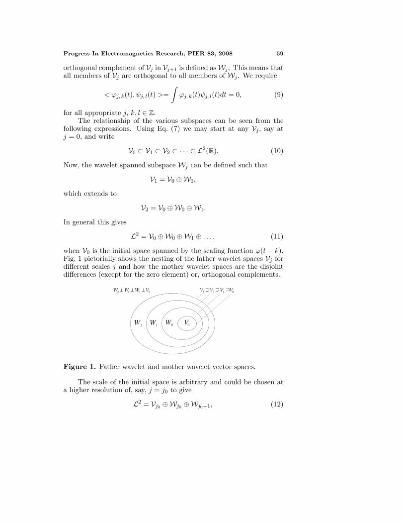
when V0 is the initial space spanned by the scaling function ϕ(t − k).Fig. 1 pictorially shows the nesting of the father wavelet spaces Vj fordifferent scales j and how the mother wavelet spaces are the disjointdifferences (except for the zero element) or, orthogonal complements.
0V0W1W2W
0123 VVVV0012 VWWW ⊃⊥ ⊥ ⊥ ⊃ ⊃
Figure 1. Father wavelet and mother wavelet vector spaces.
The scale of the initial space is arbitrary and could be chosen ata higher resolution of, say, j = j0 to give
L2 = Vj0 ⊕Wj0 ⊕Wj0+1, (12)
60 Hatamzadeh-Varmazyar et al.
or at even j = −∞ where Eq. (12) becomes
L2 = · · · ⊕W−2 ⊕W−1 ⊕W0 ⊕W1 ⊕W2 . . . (13)
Since these mother wavelets reside in the space spanned by thenext narrower father wavelet, W0 ⊂ V1, they can be represented by aweighted sum of shifted father wavelet ϕ(2t) defined in Eq. (8) by
ψ(t) =∑n∈Z
h1(n)√
2ϕ(2t − n), (14)
for some sequences of coefficients h1(n). It can be shown that themother wavelet coefficients are required by orthogonality to be relatedto the father wavelet coefficients by [58, 59]
h1(n) = (−1)nh(1 − n), (15)
the function generated by (14) gives the mother wavelet ψ(t) for a classof expansion functions of the form
ψj, k(t) = 2j/2ψ(2jt − k
), j, k ∈ Z, (16)
where, 2j is the scaling of t, 2−jk is the translation in t, and 2j/2
maintains the L2 norm of the wavelet at different scales.The set of these functions is a basis for the space of square
integrable functions L2(R), i.e.,
f(t) =∑
j
∑k
dj, kψj, k(t), f(t) ∈ L2(R). (17)
2.2. Some Properties of Wavelets
The wavelet expansion set is not unique. There are many differentwavelets systems that can be used effectively, but all seem to havesome similar characteristics [58–60].
1. All so-called first-generation wavelet systems are generated froma single scaling function (father wavelet) or mother wavelet byscaling and translation.
2. The lower resolution coefficients can be calculated from the higherresolution coefficients by a tree-structured algorithm called a filterbank. This allows a very efficient calculation of the expansioncoefficients.
Progress In Electromagnetics Research, PIER 83, 2008 61
3. Almost all useful wavelet systems satisfy the multiresolutionconditions. A multiresolution analysis (MRA) is a nestedsequence.
· · · ⊆ V−1 ⊆ V0 ⊆ V1 ⊆ V2 ⊆ . . .
of subspaces of L2(R) with a scaling function ϕ such thati)
⋃j∈Z
Vj is dense in L2(R),
ii)⋂
j∈Z
Vj = 0,
iii) f(t) ∈ Vj if and only if f(2−jt) ∈ V0, andiv) ϕ(t − k)k∈Z is an orthogonal basis for V0.
4. If the father wavelets and mother wavelets form an orthogonalbasis, there is a Parseval’s theorem that relates the energy of thesignal f(t) to the energy in each of the components and theirwavelet coefficients. That is one reason why orthogonality isimportant.
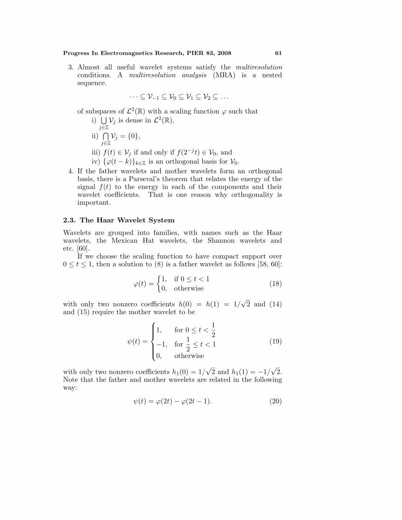
2.3. The Haar Wavelet System
Wavelets are grouped into families, with names such as the Haarwavelets, the Mexican Hat wavelets, the Shannon wavelets andetc. [60].
If we choose the scaling function to have compact support over0 ≤ t ≤ 1, then a solution to (8) is a father wavelet as follows [58, 60]:
ϕ(t) =
1, if 0 ≤ t < 10, otherwise
(18)
with only two nonzero coefficients h(0) = h(1) = 1/√
2 and (14)and (15) require the mother wavelet to be
ψ(t) =
1, for 0 ≤ t <12
−1, for12≤ t < 1
0, otherwise
(19)
with only two nonzero coefficients h1(0) = 1/√
2 and h1(1) = −1/√
2.Note that the father and mother wavelets are related in the followingway:
ψ(t) = ϕ(2t) − ϕ(2t − 1). (20)
62 Hatamzadeh-Varmazyar et al.
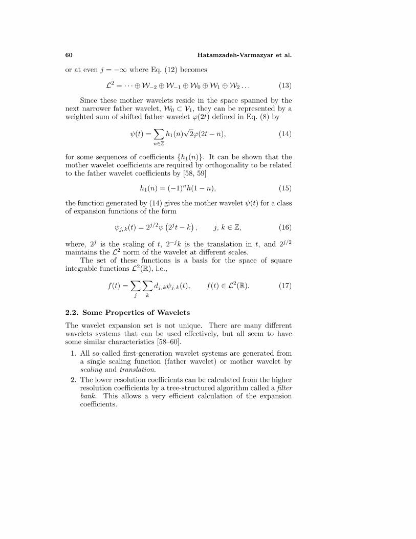
V0 is the space spanned by ϕ(t − k). The next higher resolutionspace V1 is spanned by ϕ(2t − k) which allows a somewhat moreinteresting class of functions or signals which does include V0. As weconsider higher values of scale j, the space Vj spanned by ϕ(2jt − k)becomes more suitable to approximate arbitrary functions or signals.
The Haar wavelets are illustrated in Fig. 2 that shows clearly howincreasing the scale allows greater and greater detail to be realized.
0
1
2
3
4
5
6
7
3210kj
)2( ktj -ϕ
0V 1V 2V 3V
Figure 2. Haar scaling functions that span Vj .
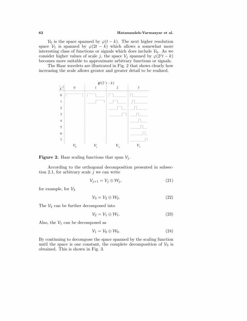
According to the orthogonal decomposition presented in subsec-tion 2.1, for arbitrary scale j we can write
Vj+1 = Vj ⊕Wj , (21)
for example, for V3
V3 = V2 ⊕W2. (22)
The V2 can be further decomposed into
V2 = V1 ⊕W1. (23)
Also, the V1 can be decomposed as
V1 = V0 ⊕W0. (24)
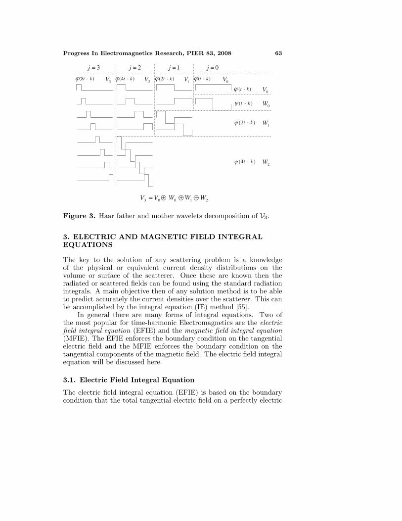
By continuing to decompose the space spanned by the scaling functionuntil the space is one constant, the complete decomposition of V3 isobtained. This is shown in Fig. 3.
Progress In Electromagnetics Research, PIER 83, 2008 63
)8( kt -ϕ )4( kt -ϕ )2( kt -ϕ )( kt -ϕ
)( kt -ϕ
)( kt
)2( ktψ
)4( kt -ψ
3V 2V 1V 0V
0V
0W
1W
2W
21003 WWWVV =
3=j 2=j 1=j 0=j
⊗ ⊗ ⊗
-
-ψ
Figure 3. Haar father and mother wavelets decomposition of V3.
3. ELECTRIC AND MAGNETIC FIELD INTEGRALEQUATIONS
The key to the solution of any scattering problem is a knowledgeof the physical or equivalent current density distributions on thevolume or surface of the scatterer. Once these are known then theradiated or scattered fields can be found using the standard radiationintegrals. A main objective then of any solution method is to be ableto predict accurately the current densities over the scatterer. This canbe accomplished by the integral equation (IE) method [55].
In general there are many forms of integral equations. Two ofthe most popular for time-harmonic Electromagnetics are the electricfield integral equation (EFIE) and the magnetic field integral equation(MFIE). The EFIE enforces the boundary condition on the tangentialelectric field and the MFIE enforces the boundary condition on thetangential components of the magnetic field. The electric field integralequation will be discussed here.
3.1. Electric Field Integral Equation
The electric field integral equation (EFIE) is based on the boundarycondition that the total tangential electric field on a perfectly electric
64 Hatamzadeh-Varmazyar et al.
conducting (PEC) surface of scatterer is zero [55]. This can beexpressed as
Ett(r = rs) = Einc
t (r = rs) + Escatt (r = rs) = 0 on S, (25)
or
Escatt (r = rs) = −Einc
t (r = rs) on S, (26)
where, S is the conducting surface of the scatterer and r = rs isthe position vector of any point on the surface of the scatterer. Thesubscript t indicates tangential components.
The incident field that impinges on the surface of the scattererinduces on it an electric current density Js which in turn radiates thescattered field. The scattered field everywhere can be found using thefollowing equation [55]:
Escat(r)=−jωA − j1
ωµε∇(∇ · A)=−j
1ωµε
[ω2µεA + ∇(∇ · A)
],
(27)
where,ε, is the permittivity of the medium;µ, is the permeability of the medium;ω, is the angle frequency of the incident field;∇, is the gradient operator;A, is the magnetic vector potential, so that
A(r) = µ
∫ ∫SJs(r′)
e−jβR
4πRds′, (28)
where, R is the distance from source point to the observation point.Equations (27) and (28) can also be expressed as [55]
Escat (r)=−jη
β
[β2
∫∫SJs
(r′
)G
(r, r′
)ds′+∇
∫∫S∇′ · Js
(r′
)G
(r, r′
)ds′
],
(29)
where, η is the intrinsic impedance of the medium and β is the phaseconstant; r and r′ are the position vectors of the observation point andsource point respectively. also,
G(r, r′
)=
e−jβR
4πR, (30)
R = |r − r′|. (31)
Progress In Electromagnetics Research, PIER 83, 2008 65
In Eq. (29), ∇ and ∇′ are, respectively, the gradients with respect tothe observation and source coordinates and G(r, r′) is referred to asGreen’s function for a three-dimensional scatterer.
If the observations are restricted on the surface of the scatterer(r = rs), then Eq. (29) through Eq. (31) can be expressed usingEq. (26) as
jη
β
[β2
∫ ∫SJs
(r′
)G
(rs, r′
)ds′ + ∇
∫ ∫S∇′ · Js
(r′
)G
(rs, r′
)ds′
]
=Einct (r = rs) . (32)
Because the right side of Eq. (32) is expressed in terms of the knownincident electric field, it is referred to as the electric field integralequation (EFIE). It can be used to find the current density Js(r′)at any point r = r′ on the scatterer. It should be noted that Eq. (32)is actually an integro-differential equation, but usually it is referred toas an integral equation.
Equation (32) is a general surface EFIE for three-dimensionalproblems and its form can be simplified for two-dimensional geometries.Note that this equation gives the EFIE for conducting surfaces. EFIEfor the resistive surfaces will be described in detail in Section 5.
4. IMPLEMENTING THE METHOD OF MOMENTSUSING HAAR WAVELETS
In this section, we apply Haar wavelets as orthogonal basis functionsto solve the integral equations of the second kind by moments method.
Consider the following Fredholm integral equation of the secondkind:
x(s) +∫ b
ak(s, t)x(t)dt = y(s), (33)
where, k(s, t) and y(s) are known functions but x(t) is unknown. Wecan select a sequence of finite dimensional subspaces Vj ⊂ L2(R), j ≥ 1.Let ϕn, kn
k=1 be a wavelet basis for Vj in which, n = 2j . Moreover,k(s, t) ∈ L2([a, b) × [a, b)) and y(s) ∈ L2([a, b)). Approximating thefunction x(s) with respect to the basis functions by (6) gives
x(s) n∑
k=1
ckϕn, k(s), (34)
such that the cks are wavelet coefficients of x(s) that should bedetermined.
66 Hatamzadeh-Varmazyar et al.
Substituting Eq. (34) into (33) follows:
n∑k=1
ckϕn, k(s) +n∑
k=1
ck
∫ b
ak(s, t)ϕn, k(t)dt y(s). (35)
Now, let si, i = 1, 2, . . . , n, be n appropriate points in interval[a, b); putting s = si in Eq. (35) follows:
n∑k=1
ckϕn, k(si) +n∑
k=1
ck
∫ b
ak(si, t)ϕn, k(t)dt y(si),
i = 1, 2, . . . , n,
(36)
orn∑
k=1
ck
[ϕn, k(si) +
∫ b
ak(si, t)ϕn, k(t)dt
] y(si),
i = 1, 2, . . . , n.
(37)
Now, replace with =, hence Eq. (37) is a linear system of nalgebraic equations for n unknown coefficients c1, c2, . . . , cn. So, anapproximate solution x(s) ∑n
k=1 ckϕn, k(s), is obtained for Eq. (33).
5. CALCULATING THE RADAR CROSS SECTION OFTHE RESISTIVE STRIPS
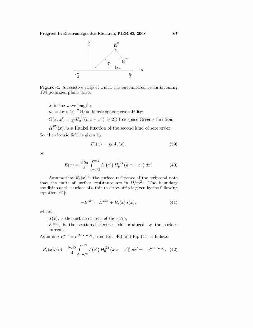
Now, the problem of calculating the RCS of the resistive strips is solvedusing the presented approach. In Fig. 4, there is a resistive strip that isvery long in the ±z direction. This strip is encountered by an incomingplane wave that has a polarization with its electric field parallel to thez-axis. The magnetic field of this wave is entirely in the x-y plane, andis therefore transverse to the z-axis. It is called transverse magnetic(TM) polarized wave. This polarization therefore produces a currenton the strip that flows along the z-axis.
The magnetic vector potential of the current flowing along thestrip is given by [61]
Az =µ0
4j
∫ a/2
−a/2Iz
(x′)H
(2)0
(k|x − x′|
)dx′, (38)
where,
k = 2πλ , is free space wave number;
Progress In Electromagnetics Research, PIER 83, 2008 67
x
y
2a
2a-
inc
ZE
incH
ZI0φ
→
→
→
Figure 4. A resistive strip of width a is encountered by an incomingTM-polarized plane wave.
λ, is the wave length;µ0 = 4π × 10−7 H/m, is free space permeability;
G(x, x′) = 14j H
(2)0 (k|x − x′|), is 2D free space Green’s function;
H(2)0 (x), is a Hankel function of the second kind of zero order.
So, the electric field is given by
Ez(x) = jωAz(x), (39)
or
E(x) =ωµ0
4
∫ a/2
−a/2Iz
(x′)H
(2)0
(k|x − x′|
)dx′. (40)
Assume that Rs(x) is the surface resistance of the strip and notethat the units of surface resistance are in Ω/m2. The boundarycondition at the surface of a thin resistive strip is given by the followingequation [61]:
−Einc = Escat + Rs(x)J(x), (41)
where,
J(x), is the surface current of the strip;Escat, is the scattered electric field produced by the surfacecurrent.
Assuming Einc = ejkx cos φ0 , from Eq. (40) and Eq. (41) it follows:
Rs(x)I(x) +ωµ0
4
∫ a/2
−a/2I
(x′)H
(2)0
(k|x − x′|
)dx′ = −ejkx cos φ0 , (42)
68 Hatamzadeh-Varmazyar et al.
where, I(x) is the current of the strip.Equation (42) can be converted to the following equation:
h(x) +∫ b
aG
(x, x′)h
(x′) dx′ = g(x), (43)
where,h(x) = I(x);
G(x, x′) = ωµ0
41
Rs(x)H(2)0 (k|x − x′|);
g(x) = − 1Rs(x)e
jkx cos φ0 .
It is a Fredholm integral equation of the second kind and can besolved by the presented method. However, from Eq. (42) I(x) can beobtained and then the RCS of the strip can be computed easily.
RCS in two dimensions is defined mathematically as [61]
σ(φ) = limr→∞
2πr|Escat|2|Einc|2 . (44)
In two dimensions, the free space Green’s function is
G(r, r′
)=
14j
H(2)0
(k|r − r′|
). (45)
The magnetic vector potential in two-dimensional space is
A(r) = µ
∫∫J
(r′
)G
(r, r′
)ds′. (46)
The electric field is given by
E = jωA. (47)
Combining (45), (46), and (47) we obtain
E(r) =ωµ
4
∫∫J
(r′
)H
(2)0
(k|r − r′|
)ds′. (48)
In the TM situation, the incident electric field along the strip is1 V/m (|Einc|2 = 1). So, the denominator of Eq. (44) is unity. Thisallows us to turn our attention to the numerator. To evaluate (48), wenote that as r −→ ∞, we can use the large argument approximationfor the Hankel function [61]
H(2)0 (r) ≈
√2πr
e−j(r−π4 ). (49)
Progress In Electromagnetics Research, PIER 83, 2008 69
Substituting this into (48) and implementing Eq. (44) for the TMcase, we obtain
σ(φ) =kη2
4
∣∣∣∣∫
stripI
(x′, y′
)ejk(x′ cos φ+y′ sin φ)dl′
∣∣∣∣2
. (50)
where, η = 376.73 Ω.In the presented case, the strip is restricted to the x-axis, which
simplifies Eq. (50)
σ(φ) =kη2
4
∣∣∣∣∣∫ a/2
−a/2I
(x′) ejkx′ cos φdx′
∣∣∣∣∣2
. (51)
Also, it is possible to define a logarithmic quantity with respectto the RCS, so that
σdBlm = 10 log10 σ. (52)
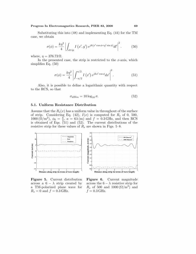
5.1. Uniform Resistance Distribution
Assume that the Rs(x) has a uniform value in throughout of the surfaceof strip. Considering Eq. (42), I(x) is computed for Rs of 0, 500,1000 (Ω/m2), φ0 = π
2 , a = 6λ (m) and f = 0.3 GHz, and then RCSis obtained of Eqs. (51) and (52). The current distributions of theresistive strip for these values of Rs are shown in Figs. 5–8.
-3 -2 -1 0 1 2 3-15
-10
-5
0
5
10
15
Distance along strip (in trems of wave length)
Cur
rent
(m
A/m
)
Magnitude
Real
Imaginary
Figure 5. Current distributionacross a 6 − λ strip created bya TM-polarized plane wave forRs = 0 and f = 0.3 GHz.
-3 -2 -1 0 1 2 30.8
0.9
1
1.1
1.2
1.3
1.4
1.5
1.6
1.7
1.8
Distance along strip (in terms of wave length)
Cur
rent
(m
agni
tude
, mA
/m) 500 Ohms/m2
1000 Ohms/m2
Figure 6. Current magnitudeacross the 6 − λ resistive strip forRs of 500 and 1000 (Ω/m2) andf = 0.3 GHz.
70 Hatamzadeh-Varmazyar et al.
-3 -2 -1 0 1 2 3-1. 7
-1. 6
-1. 5
-1. 4
-1. 3
-1. 2
-1. 1
-1
-0. 9
-0. 8
Distance along strip (in terms of wave length)
Cur
rent
(re
al p
art,
mA
/m)
500 Ohms/m2
1000 Ohms/m2
Figure 7. The real part of cur-rent across the 6−λ resistive stripfor Rs of 500 and 1000 (Ω/m2)and f = 0.3 GHz.
-3 -2 -1 0 1 2 3-0. 1
-0.05
0
0.05
0.1
0.15
0.2
0.25
Distance along strip (in terms of wave length)
Cur
rent
(im
agin
ary
part
, mA
/m)
500 Ohms/m2
1000 Ohms/m2
Figure 8. The imaginary partof current across the 6 − λresistive strip for Rs of 500 and1000 (Ω/m2) and f = 0.3 GHz.
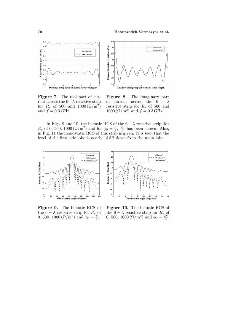
In Figs. 9 and 10, the bistatic RCS of the 6− λ resistive strip, forRs of 0, 500, 1000 (Ω/m2) and for φ0 = π
2 , 2π3 has been shown. Also,
in Fig. 11 the monostatic RCS of this strip is given. It is seen that thelevel of the first side lobe is nearly 13 dB down from the main lobe.
0 20 40 60 80 100 120 140 160 180- 40
-30
-20
-10
0
10
20
30
Observation angle (degrees)
Bis
tati
c R
CS
(dB
lm)
0 Ohms/m2
500 Ohms/m2
1000 Ohms/m2
Figure 9. The bistatic RCS ofthe 6 − λ resistive strip for Rs of0, 500, 1000 (Ω/m2) and φ0 = π
2 .
0 20 40 60 80 100 120 140 160 180-50
-40
-30
-20
-10
0
10
20
30
Observation angle (degrees)
Bis
tati
c R
CS
(dB
lm)
0 Ohms/m2
500 Ohms/m2
1000 Ohms/m2
Figure 10. The bistatic RCS ofthe 6 − λ resistive strip for Rs of0, 500, 1000 (Ω/m2) and φ0 = 2π
3 .
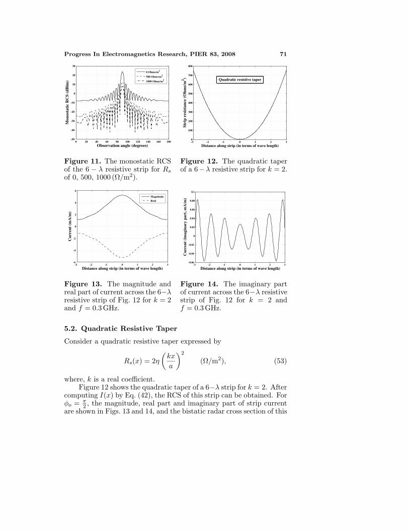
Progress In Electromagnetics Research, PIER 83, 2008 71
0 20 40 60 80 100 120 140 160 180-50
-40
-30
-20
-10
0
10
20
30
Observation angle (degrees)
Mon
osta
tic
RC
S (d
Blm
)0 Ohms/m2
500 Ohms/m2
1000 Ohms/m2
Figure 11. The monostatic RCSof the 6 − λ resistive strip for Rs
of 0, 500, 1000 (Ω/m2).
-3 -2 -1 0 1 2 30
100
200
300
400
500
600
700
800
Distance along strip (in terms of wave length)
Stri
p re
sist
ance
(O
hms/
m2 ) Quadratic resistive taper
Figure 12. The quadratic taperof a 6−λ resistive strip for k = 2.
-3 -2 -1 0 1 2 3-6
-4
-2
0
2
4
6
Distance along strip (in terms of wave length)
Cur
rent
(m
A/m
)
Magnitude
Real
Figure 13. The magnitude andreal part of current across the 6−λresistive strip of Fig. 12 for k = 2and f = 0.3 GHz.
-3 -2 -1 0 1 2 3-0.06
-0.04
-0.02
0
0.02
0.04
0.06
0.08
0.1
Distance along strip (in terms of wave length)
Cur
rent
(im
agin
ary
part
, mA
/m)
Figure 14. The imaginary partof current across the 6−λ resistivestrip of Fig. 12 for k = 2 andf = 0.3 GHz.
5.2. Quadratic Resistive Taper
Consider a quadratic resistive taper expressed by
Rs(x) = 2η(
kx
a
)2
(Ω/m2), (53)
where, k is a real coefficient.Figure 12 shows the quadratic taper of a 6−λ strip for k = 2. After
computing I(x) by Eq. (42), the RCS of this strip can be obtained. Forφo = π
2 , the magnitude, real part and imaginary part of strip currentare shown in Figs. 13 and 14, and the bistatic radar cross section of this
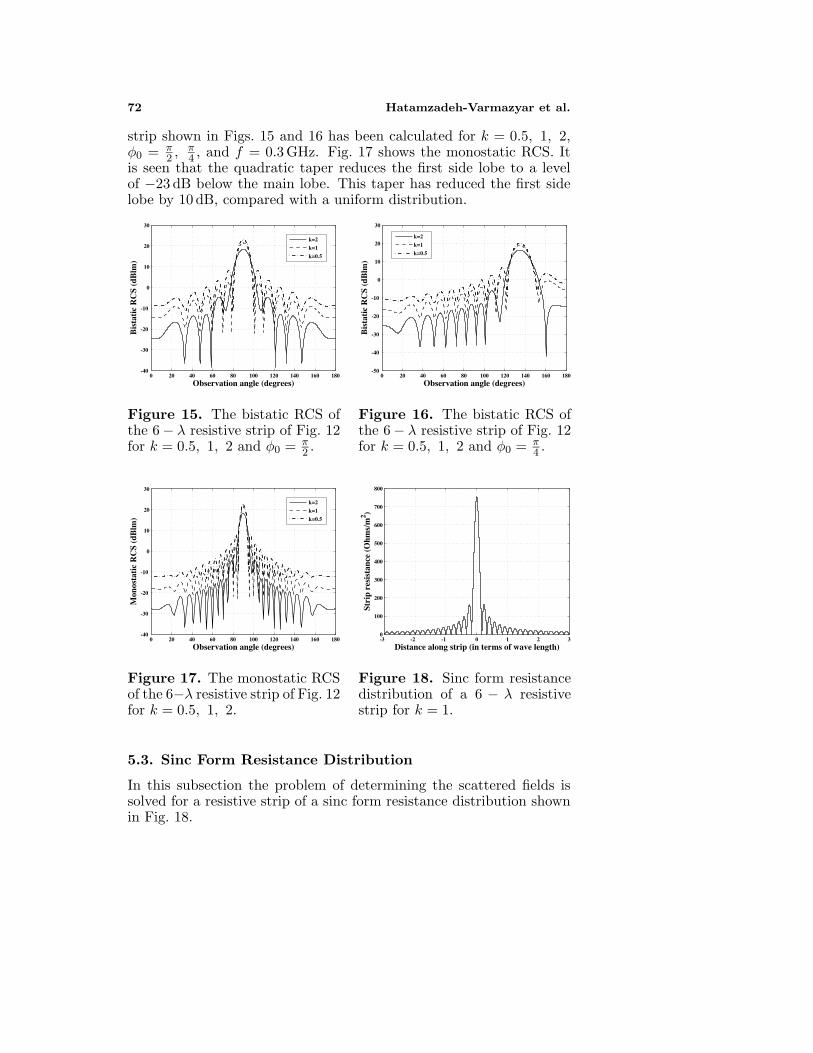
72 Hatamzadeh-Varmazyar et al.
strip shown in Figs. 15 and 16 has been calculated for k = 0.5, 1, 2,φ0 = π
2 , π4 , and f = 0.3 GHz. Fig. 17 shows the monostatic RCS. It
is seen that the quadratic taper reduces the first side lobe to a levelof −23 dB below the main lobe. This taper has reduced the first sidelobe by 10 dB, compared with a uniform distribution.
0 20 40 60 80 100 120 140 160 180-40
-30
-20
-10
0
10
20
30
Observation angle (degrees)
Bis
tati
c R
CS
(dB
lm)
k=2
k=1
k=0.5
Figure 15. The bistatic RCS ofthe 6− λ resistive strip of Fig. 12for k = 0.5, 1, 2 and φ0 = π
2 .
0 20 40 60 80 100 120 140 160 180-50
-40
-30
-20
-10
0
10
20
30
Observation angle (degrees)
Bis
tati
c R
CS
(dB
lm)
k=2
k=1
k=0.5
Figure 16. The bistatic RCS ofthe 6− λ resistive strip of Fig. 12for k = 0.5, 1, 2 and φ0 = π
4 .
0 20 40 60 80 100 120 140 160 180-40
-30
-20
-10
0
10
20
30
Observation angle (degrees)
Mon
osta
tic
RC
S (d
Blm
)
k=2
k=1
k=0.5
Figure 17. The monostatic RCSof the 6−λ resistive strip of Fig. 12for k = 0.5, 1, 2.
-3 -2 -1 0 1 2 30
100
200
300
400
500
600
700
800
Distance along strip (in terms of wave length)
Stri
p re
sist
ance
(O
hms/
m2 )
Figure 18. Sinc form resistancedistribution of a 6 − λ resistivestrip for k = 1.
5.3. Sinc Form Resistance Distribution
In this subsection the problem of determining the scattered fields issolved for a resistive strip of a sinc form resistance distribution shownin Fig. 18.
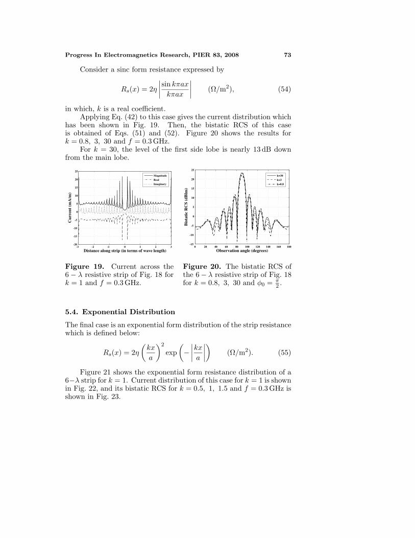
Progress In Electromagnetics Research, PIER 83, 2008 73
Consider a sinc form resistance expressed by
Rs(x) = 2η∣∣∣∣sin kπax
kπax
∣∣∣∣ (Ω/m2), (54)
in which, k is a real coefficient.Applying Eq. (42) to this case gives the current distribution which
has been shown in Fig. 19. Then, the bistatic RCS of this caseis obtained of Eqs. (51) and (52). Figure 20 shows the results fork = 0.8, 3, 30 and f = 0.3 GHz.
For k = 30, the level of the first side lobe is nearly 13 dB downfrom the main lobe.
-3 -2 -1 0 1 2 3-20
-15
-10
-5
0
5
10
15
20
25
Distance along strip (in terms of wave length)
Cur
rent
(m
A/m
)
Magnitude
Real
Imaginary
Figure 19. Current across the6 − λ resistive strip of Fig. 18 fork = 1 and f = 0.3 GHz.
0 20 40 60 80 100 120 140 160 180-15
-10
-5
0
5
10
15
20
25
Observation angle (degrees)
Bis
tati
c R
CS
(dB
lm)
k=30
k=3
k=0.8
Figure 20. The bistatic RCS ofthe 6− λ resistive strip of Fig. 18for k = 0.8, 3, 30 and φ0 = π
2 .
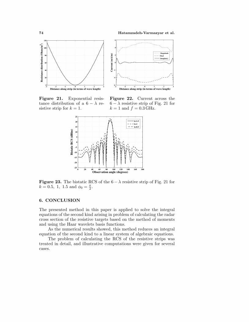
5.4. Exponential Distribution
The final case is an exponential form distribution of the strip resistancewhich is defined below:
Rs(x) = 2η(
kx
a
)2
exp(−
∣∣∣∣kx
a
∣∣∣∣)
(Ω/m2). (55)
Figure 21 shows the exponential form resistance distribution of a6−λ strip for k = 1. Current distribution of this case for k = 1 is shownin Fig. 22, and its bistatic RCS for k = 0.5, 1, 1.5 and f = 0.3 GHz isshown in Fig. 23.
74 Hatamzadeh-Varmazyar et al.
-3 -2 -1 0 1 2 30
20
40
60
80
100
120
Distance along strip (in terms of wave length)
Res
ista
nce
dist
ribu
tion
(O
hms/
m2 )
Figure 21. Exponential resis-tance distribution of a 6 − λ re-sistive strip for k = 1.
-3 -2 -1 0 1 2 3-6
-4
-2
0
2
4
6
Distance along strip (in terms of wave length)
Cur
rent
(m
A/m
) Magnitude
Real
Imaginary
Figure 22. Current across the6 − λ resistive strip of Fig. 21 fork = 1 and f = 0.3 GHz.
0 20 40 60 80 100 120 140 160 180-25
-20
-15
-10
-5
0
5
10
15
20
25
Observation angle (degrees)
Bis
tati
c R
CS
(dB
lm)
k=1.5
k=1
k=0.5
Figure 23. The bistatic RCS of the 6− λ resistive strip of Fig. 21 fork = 0.5, 1, 1.5 and φ0 = π
2 .
6. CONCLUSION
The presented method in this paper is applied to solve the integralequations of the second kind arising in problem of calculating the radarcross section of the resistive targets based on the method of momentsand using the Haar wavelets basis functions.
As the numerical results showed, this method reduces an integralequation of the second kind to a linear system of algebraic equations.
The problem of calculating the RCS of the resistive strips wastreated in detail, and illustrative computations were given for severalcases.
Progress In Electromagnetics Research, PIER 83, 2008 75
A comparison of the method presented here with other methodsthat we have implemented using the block-pulse or triangular basisfunctions [28,31] shows the accuracy and validity of the presentedmethod.
This method can be easily generalized to apply to objects ofarbitrary geometry and arbitrary material.
REFERENCES
1. Wilton, D. R. and C. M. Butler, “Effective methods for solvingintegral and integro-differential equations,” Electromagnetics,Vol. 1, 289–308, 1981.
2. Harrington, R. F., “Matrix methods for field problems,” Proc.IEEE , Vol. 55, No. 2, 136–149, 1967.
3. Mishra, M. and N. Gupta, “Monte Carlo integration techniquefor the analysis of electromagnetic scattering from conductingsurfaces,” Progress In Electromagnetics Research, PIER 79, 91–106, 2008.
4. Arnold, M. D., “An efficient solution for scattering by a perfectlyconducting strip grating,” Journal of Electromagnetic Waves andApplications, Vol. 20, No. 7, 891–900, 2006.
5. Zhao, J. X., “Numerical and analytical formulations of theextended MIE theory for solving the sphere scattering problem,”Journal of Electromagnetic Waves and Applications, Vol. 20,No. 7, 967–983, 2006.
6. Ruppin, R., “Scattering of electromagnetic radiation by a perfectelectromagnetic conductor sphere,” Journal of ElectromagneticWaves and Applications, Vol. 20, No. 12, 1569–1576, 2006.
7. Ruppin, R., “Scattering of electromagnetic radiation by a perfectelectromagnetic conductor cylinder,” Journal of ElectromagneticWaves and Applications, Vol. 20, No. 13, 1853–1860, 2006.
8. Hussein, K. F. A., “Efficient near-field computation for radiationand scattering from conducting surfaces of arbitrary shape,”Progress In Electromagnetics Research, PIER 69, 267–285, 2007.
9. Hussein, K. F. A., “Fast computational algorithm for EFIEapplied to arbitrarily-shaped conducting surfaces,” Progress InElectromagnetics Research, PIER 68, 339–357, 2007.
10. Kishk, A. A., “Electromagnetic scattering from composite objectsusing a mixture of exact and impedance boundary conditions,”IEEE Transactions on Antennas and Propagation, Vol. 39, No. 6,826–833, 1991.
76 Hatamzadeh-Varmazyar et al.
11. Caorsi, S., A. Massa, and M. Pastorino, “A numerical solutionto full-vector electromagnetic scattering by three-dimensionalnonlinear bounded dielectrics,” IEEE Transactions on MicrowaveTheory and Techniques, Vol. 43, No. 2, 428–436, 1995.
12. Shore, R. A. and A. D. Yaghjian, “Dual-surface integral equationsin electromagnetic scattering,” IEEE Transactions on Antennasand Propagation, Vol. 53, No. 5, 1706–1709, 2005.
13. Yla-Oijala, P. and M. Taskinen, “Well-conditioned Mullerformulation for electromagnetic scattering by dielectric objects,”IEEE Transactions on Antennas and Propagation, Vol. 53, No. 10,3316–3323, 2005.
14. Li, L. W., P. S. Kooi, Y. L. Qin, T. S. Yeo, and M. S. Leong,“Analysis of electromagnetic scattering of conducting circular diskusing a hybrid method,” Progress In Electromagnetics Research,PIER 20, 101–123, 1998.
15. Liu, Y. and K. J. Webb, “On detection of the interior resonanceerrors of surface integral boundary conditions for electromagneticscattering problems,” IEEE Transactions on Antennas andPropagation, Vol. 49, No. 6, 939–943, 2001.
16. Kishk, A. A., “Electromagnetic scattering from transverselycorrugated cylindrical structures using the asymptotic corrugatedboundary conditions,” IEEE Transactions on Antennas andPropagation, Vol. 52, No. 11, 3104–3108, 2004.
17. Tong, M. S. and W. C. Chew, “Nystrom method with edgecondition for electromagnetic scattering by 2D open structures,”Progress In Electromagnetics Research, PIER 62, 49–68, 2006.
18. Valagiannopoulos, C. A., “Closed-form solution to the scatteringof a skew strip field by metallic pin in a slab,” Progress InElectromagnetics Research, PIER 79, 1–21, 2008.
19. Frangos, P. V. and D. L. Jaggard, “Analytical and numericalsolution to the two-potential Zakharov-Shabat inverse scatteringproblem,” IEEE Transactions on Antennas and Propagation,Vol. 40, No. 4, 399–404, 1992.
20. Barkeshli, K. and J. L. Volakis, “Electromagnetic scattering fromthin strips — Part II: Numerical solution for strips of arbitrarysize,” IEEE Transactions on Education, Vol. 47, No. 1, 107–113,2004.
21. Collino, F., F. Millot, and S. Pernet, “Boundary-integral methodsfor iterative solution of scattering problems with variableimpedance surface condition,” Progress In ElectromagneticsResearch, PIER 80, 1–28, 2008.
Progress In Electromagnetics Research, PIER 83, 2008 77
22. Zahedi, M. M. and M. S. Abrishamian, “Scattering fromsemi-elliptic channel loaded with impedance elliptical cylinder,”Progress In Electromagnetics Research, PIER 79, 47–58, 2008.
23. Zaki, K. A. and A. R. Neureuther, “Scattering from aperfectly conducting surface with a sinusoidal height profile: TEpolarization,” IEEE Transactions on Antennas and Propagation,Vol. 19, No. 2, 208–214, 1971.
24. Carpentiery, B., “Fast iterative solution methods in electro-magnetic scattering,” Progress In Electromagnetics Research,PIER 79, 151–178, 2008.
25. Du, Y., Y. L. Luo, W. Z. Yan, and J. A. Kong, “Anelectromagnetic scattering model for soybean canopy,” ProgressIn Electromagnetics Research, PIER 79, 209–223, 2008.
26. Umashankar, K. R., S. Nimmagadda, and A. Taflove, “Numericalanalysis of electromagnetic scattering by electrically large objectsusing spatial decomposition technique,” IEEE Transactions onAntennas and Propagation, Vol. 40, No. 8, 867–877, 1992.
27. Gokten, M., A. Z. Elsherbeni, and E. Arvas, “Electromagneticscattering analysis using the two-dimensional MRFD formula-tion,” Progress In Electromagnetics Research, PIER 79, 387–399,2008.
28. Hatamzadeh-Varmazyar, S., M. Naser-Moghadasi, E. Babo-lian, and Z. Masouri, “Numerical approach to survey the problemof electromagnetic scattering from resistive strips based on usinga set of orthogonal basis functions,” Progress In ElectromagneticsResearch, PIER 81, 393–412, 2008.
29. Hatamzadeh-Varmazyar, S., M. Naser-Moghadasi, and Z. Ma-souri, “A moment method simulation of electromagnetic scatter-ing from conducting bodies,” Progress In Electromagnetics Re-search, PIER 81, 99–119, 2008.
30. Hatamzadeh-Varmazyar, S. and M. Naser-Moghadasi, “Newnumerical method for determining the scattered electromagneticfields from thin wires,” Progress In Electromagnetics Research B ,Vol. 3, 207–218, 2008.
31. Hatamzadeh-Varmazyar, S. and M. Naser-Moghadasi, “Anintegral equation modeling of electromagnetic scattering fromthe surfaces of arbitrary resistance distribution,” Progress InElectromagnetics Research B , Vol. 3, 157–172, 2008.
32. Abd-El-Ranouf, H. E. and R. Mittra, “Scattering analysis ofdielectric coated cones,” Journal of Electromagnetic Waves andApplications, Vol. 21, No. 13, 1857–1871, 2007.
78 Hatamzadeh-Varmazyar et al.
33. Choi, S. and N.-H. Myung, “Scattering analysis of open-endedcavity with inner object,” Journal of Electromagnetic Waves andApplications, Vol. 21, No. 12, 1689–1702, 2007.
34. Li, Y.-L., J.-Y. Huang, and S.-H. Gong, “The scattering crosssection for a target irradiated by time-varying electromagneticwaves,” Journal of Electromagnetic Waves and Applications,Vol. 21, No. 9, 1265–1271, 2007.
35. Rui, P.-L. and R. Chen, “Implicity restarted gmres fast Fouriertransform method for electromagnetic scattering,” Journal ofElectromagnetic Waves and Applications, Vol. 21, No. 7, 973–976,2007.
36. Nashia, N., J. S. Kot, and S. S. Vinogradov, “Scattering by aluneberg lens partially covered by a metallic cap,” Journal ofElectromagnetic Waves and Applications, Vol. 21, No. 4, 549–563,2007.
37. Yuan, H.-W., S.-X. Gong, X. Wang, and W.-T. Wang, “Scatteringanalysis of a printed dipole antenna using PBG structures,”Progress In Electromagnetics Research B , Vol. 1, 189–195, 2008.
38. Faghihi, F. and H. Heydari, “A combination of time domain finiteelement-boundary integral and with time domain physical opticsfor calculation of electromagnetic scattering of 3-D structures,”Progress In Electromagnetics Research, PIER 79, 463–474, 2008.
39. Ahmed, S. and Q. A. Naqavi, “Electromagnetic scattering from aperfect electromagnetic conductor cylinder buried in a dielectrichalf-space,” Progress In Electromagnetics Research, PIER 78, 25–38, 2008.
40. Valagiannopoulos, C. A., “Electromagnetic scattering from twoeccentric metamaterial cylinders with frequency-dependent per-mittivities differing slightly each other,” Progress In Electromag-netics Research B , Vol. 3, 23–34, 2008.
41. Hady, L. K. and A. A. Kishk, “Electromagnetic scatteringfrom conducting circular cylinder coated by meta-materials andloaded with helical strips under oblique incidence,” Progress InElectromagnetics Research B , Vol. 3, 189–206, 2008.
42. Zainud-Deen, S. H., A. Z. Botros, and M. S. Ibrahim, “Scatteringfrom bodies coated with metamaterial using FDFD method,”Progress In Electromagnetics Research B , Vol. 2, 279–290, 2008.
43. Li, Y.-L., J.-Y. Huang, M.-J. Wang, and J. Zhang, “Scatteringfield for the ellipsoidal targets irradiated by an electromagneticwave with arbitrary polarizing and propagating direction,”Progress In Electromagnetics Research Letters, Vol. 1, 221–235,2008.
Progress In Electromagnetics Research, PIER 83, 2008 79
44. Xu, L., Y.-C. Guo, and X.-W. Shi, “Dielectric half space model forthe analysis of scattering from objects on ocean surface,” Journalof Electromagnetic Waves and Applications, Vol. 21, No. 15, 2287–2296, 2007.
45. Zhong, X. J., T. Cui, Z. Li, Y.-B. Tao, and H. Lin, “Terahertz-wave scattering by perfectly electrical conducting objects,”Journal of Electromagnetic Waves and Applications, Vol. 21,No. 15, 2331–2340, 2007.
46. Li, Y.-L., J.-Y. Huang, and M.-J. Wang, “Scattering cross sectionfor airborne and its application,” Journal of ElectromagneticWaves and Applications, Vol. 21, No. 15, 2341–2349, 2007.
47. Wang, M. Y., J. Xu, J. Wu, Y. Yan, and H.-L. Li, “FDTDstudy on scattering of metallic column covered by double-negative metamaterial,” Journal of Electromagnetic Waves andApplications, Vol. 21, No. 14, 1905–1914, 2007.
48. Liu, X.-F., B. Z. Wang, and S.-J. Lai, “Element-free Galerkinmethod in electromagnetic scattering field computation,” Journalof Electromagnetic Waves and Applications, Vol. 21, No. 14, 1915–1923, 2007.
49. Du, P., B. Z. Wang, H. Li, and G. Zheng, “Scattering analysis oflarge-scale periodic structures using the sub-entire domain basisfunction method and characteristic function method,” Journal ofElectromagnetic Waves and Applications, Vol. 21, No. 14, 2085–2094, 2007.
50. Tuz, V. R., “Three-dimensional Gaussian beam scattering from aperiodic sequence of bi-isotropic and material layers,” Progress InElectromagnetics Research B , Vol. 7, 53–73, 2008.
51. Sukharevsky, O. I. and V. A. Vasilets, “Scattering of reflector an-tenna with conic dielectric radome,” Progress In ElectromagneticsResearch B , Vol. 4, 159–169, 2008.
52. Wang, M.-J., Z.-S. Wu, and Y. L. Li, “Investigation on thescattering characteristics of Gaussian beam from two dimensionaldielectric rough surfaces based on the Kirchhoff approximation,”Progress In Electromagnetics Research B , Vol. 4, 223–235, 2008.
53. Sun, X. and H. Ha, “Light scattering by large hexagonalcolumn with multiple densely packed inclusions,” Progress InElectromagnetics Research Letters, Vol. 3, 105–112, 2008.
54. Kokkorakis, G. C., “Scalar equations for scattering by rotationallysymmetric radially inhomogeneous anisotropic sphere,” ProgressIn Electromagnetics Research Letters, Vol. 3, 179–186, 2008.
55. Balanis, C. A., Advanced Engineering Electromagnetics, Wiley,
80 Hatamzadeh-Varmazyar et al.
New York, 1989.56. Balanis, C. A., Antenna Theory: Analysis and Design, Wiley,
New York, 1982.57. Delves, L. M. and J. L. Mohamed, Computational Methods for
Integral Equations, Cambridge University Press, Cambridge, 1985.58. Burrus, C. S., R. A. Gopinath, and H. Guo, Introduction to
Wavelets and Wavelet Transforms, New Jersey, Prentice Hall,1998.
59. Daubechies, I., Ten Lectures on Wavelets, SIAM, Philadelphia,1992.
60. Aboufadel, E. and S. Schlicker, Discovering Wavelets, John Wiley& Sons, 1999.
61. Bancroft, R., Understanding Electromagnetic Scattering Using theMoment Method , Artech House, London, 1996.