Calculation of Carbonaceous Overlayer Thickness in XPS to Yield Substrate Stoichiometries
L E E GRIFFITHS* and L E S B R A D L E Y ICI Chemicals & Polymers Ltd., Research & Technology Department, P.O. Box 8, The Heath, Runcorn, Cheshire, WA7 4QD, U.K.
A method has been developed which calculates the thickness of the hydrocarbon overlayer from x-ray photoemission spectroscopy (XPS) spectra. The method is specific to each sample and utilizes the relative intensity of the C Is peak and all other peaks. Attenuations calculated with this overlayer thickness yield more accurate substrate stoichiom- etries. A rough-sample model is also developed which not only explains previous anomalies in the thickness of hydrocarbon overlayer calculated but is capable of yielding further accuracy in substrate stoichiometries.
Index Heading: Surface analysis.
INTRODUCTION
Surface contamination by hydrocarbons is a common problem in x-ray photoemission spectroscopy (XPS). Not only does the overlayer attenuate the intensity of pho- toelectrons emitted from below it, thus leading to poorer signal-to-noise ratios, but more seriously, the attenuation is different for varying photoelectron energies. Poor sig- nal-to-noise ratios can be improved by acquisition of spectra over longer periods of time, but the differential effect of the overlayer on different elements is not solved so readily. Some experimental procedures used to min- imize hydrocarbon overlayers are the maintenance of a good vacuum, continuous condensation of material onto a sample tip, trapping of contaminants, cleaning or scraping or cleaving of samples in vacuo, and ion etch- ing. 1
In an industrial surface science laboratory there is a need for a rapid throughput of samples, and the frequent introduction of samples makes the maintenance of a very good vacuum (< 10 -8 Torr) difficult. When oil diffusion pumps are used, a thin film of diffusion pump oil can be distributed on all samples. Furthermore, there is very little control over the initial stages of sample preparation, and samples can arrive in the laboratory seriously con- taminated.
Many such samples cannot be evaporated or cannot be assumed to be homogeneous over the depths required for scraping. Moreover, it is also possible that ion etching will cause reduction or modification of stoichiometry through preferential sputtering.
Clearly, in these cases, some other means of coping with the hydrocarbon overlayer is required. Although high-energy x-ray sources can reduce this problem, the concomitant loss of resolution and surface specificity lim- its their possible applications.
Procedures already exist for the calculation of over- layer thickness. One relies on the dependence of inten-
Received 18 August 1991; revision received 8 April 1992. * Author to whom correspondence should be sent.
sities as a function of take-off angle, 2~ but since it re- quires the spectra to be run several times, this procedure cannot be regarded as being routine. More recently, an- other method has been proposed 5,6 which allows the over- layer thickness to be calculated by comparison of the C ls peak and the KVV Auger peak, which are well sepa- rated in energy and therefore well suited to this purpose. However, the Auger peak is unlikely to allow the reso- lution of carbon in the substrate and the overlayer, how- ever, restricting the applicability of this method.
A procedure is therefore proposed which calculates the thickness of the hydrocarbon overlayer by comparing the intensities of the C ls peak of the hydrocarbon overlayer and the substrate peaks and, more importantly, yields more accurate surface stoichiometries. This method also requires that one be able to reduce a peak which is solely attributable to the hydrocarbon, but this possibility is more likely with the C ls peak than the KVV Auger peak.
THEORY
Flat Sample. It is generally assumed 7 that photoelec- trons are attenuated by inelastic scattering as given in Eq. 1:
Ij . . . . . Attj = exp(-d/X sin O) (1)
where
d
0 Ijobsd
= the depth of the overlayer, = the escape depth of the photoelectron, = the take-off angle, = the observed intensity (or area) of atom j, = the nonattenuated intensity (or area) from atom
j, and Attj = the attenuation of intensity (or area) from atom j.
It is assumed that elastic scattering is negligible 7 and therefore:
X = Xi
where Xi = inelastic mean free path of photoelectron in the given material. ~i is calculated from the equation of Seah and Dench 7 for organic compounds:
?,i = (49/E 2 + 0.11E '/2) x 13.5 (2)
where E = kinetic energy of photoelectron, and hi is given in A by using the mean density of paraffins Cs to C15 (0.74 g cm-3).
From this equation, the true intensities (or areas) can be calculated from the sample as if a uniform hydrocar- bon overlayer of given thickness were not present. How-
ever, it is necessary to know the thickness of the hydro- carbon overlayer. This problem is split into two parts: first, the thickness of a monolayer and, second, the num- ber of such monolayers must be determined.
The thickness of a monolayer a is given by the equa- tion:
a = [(MW x 1024)/NAPn] v3
where
a = the monolayer thickness (in Angstroms), MW = the molecular weight,
N = the Avagadro's number = 6.023 x 10²³ mo1-1, p = the density in kg. m -3, and n = the number of carbons per molecule.
The value of a was found to be 3.1/~ from the same series of paraffins referred to above (Cs to C15). Note this ap- proach is at variance with the relation quoted by Seah,: in which n is the number of atoms. Seah's equation nec- essarily assumes that the molecule is planar and lies flat on the surface. This assumption will lead to an under- estimate of the thickness for two reasons: the van der Waals radius of hydrogen is smaller than that for carbon, 8 and the molecule will exhibit tetrahedral oriented bond- ing. The approach in this work is to approximate the -CH2- unit to a cube, and hence n is the number of such units.
In order to calculate the number of monolayers (or total thickness) of the overlayer, consider the C ls peak of the hydrocarbon overlayer:
Ic =/coo x [1 - exp(-d/Xcsin 0)] (3)
where Ic is the observed overlayer C ls intensity (or area),
~o iS the C ls intensity (or area) that would be observed bulk hydrocarbon, and Xc is the escape depth of the
C ls photoelectron. In order to determine the hydrocarbon overlayer thick-
ness d, I~= is required. Clearly different samples will yield different numbers of photoelectrons for the same number of atoms. It is assumed that the surface roughness of the substrate, which controls the number of photoelectrons arriving at the analyzer, is exactly followed by the thin hydrocarbon overlayer and that the photoelectrons from the overlayer are dispersed in the same way. If it is fur- ther assumed that morphology does not affect the num- ber of photoelectrons, then the relative intensities from bulk substrate and overlayer are simply in the ratio of the number of atoms per unit volume. I~ ° can therefore be predicted from the substrate intensities:
Ic~ _ It~ k, (4)
where N~Sc N~S t
N~ = the number of C atoms per unit volume in the hydrocarbon overlayer,
N i = the number of j atoms per unit volume in the substrate,
S t = the appropriate relative sensitivity factor, and k~ = a constant which includes spectrometer sensitivity
and sample roughness.
The quantities N~ and N t are dependent on both the mole fraction of the element in, and the densities of, the hydrocarbon overlayer and the substrate, respectively.
The volume occupied by a -CH2- unit in the overlayer is the cube of the monolayer thickness (i.e., 29.8/~3). Since a generalized treatment is sought, the volume occupied by an atom in the substrate is assumed to be proportional to the volume occupied in a cubic packed crystal, i.e., the cube with sides twice the ionic radius:
N j = C j / ~ Ct(2rt)3 (5)
where C t is the mole fraction of atom j, and r t is the ionic radius 8 of atom j.
Substituting Eq. 5 in Eq. 4, we have:
S--~ × 29 .8 - CtSj ~ C t ( 2 r j ) 3
but since the mole fraction of each atom in the substrate is given by the de-attenuated intensities (or areas), pro- vided that one peak per element is measured:
This reduces to:
I~ It~ " (2rt)3 cS-= ~-~ S t - 29.8.
j ÷c
Substituting Eqs. 1 and 3:
I ....... [1 - exp(-d/Xcsin 0)] S~
x Sjexp(-d/Xtsin 0) + 29.8 (6)
where X is given by Eq. 2. The procedure is therefore to increase d by monolayer
increments until the calculated hydrocarbon C Is inten- sity (or area) > the observed. The corrected mole frac- tions are then given by:
It~ ~ / Ij ~ Ct = Stexp(-ff/Xtsin O) / ~ " O) Stexp(-d/k ts in •
Rough Sample. Implicit in the above treatment is the assumption that the sample is covered evenly by hydro- carbon and that it is fiat. In the case of a fiat sample, changing the "take-off angle" experimentally changes the observed stoichiometries; but after the above treat- ment, although the apparent depth of the overlayer is changed, the de-attenuated stoichiometries are not.
In the case of a rough sample, a distribution of take- off angles is introduced, and since Eq. I is nonlinear, this distribution has to be modeled exactly and cannot be compensated for by merely changing the apparent take- off angle in the fiat sample model. The other extreme, a very rough surface, must therefore be defined. We have considered such a sample as a series of spheres (partic- ularly applicable to powders).
We have assumed that:
1. The radius of the spheres is large with respect to the escape depths of the photoelectrons, and shadowing effects therefore have to be considered.
APPLIED SPECTROSCOPY 1427
A N A L Y Z E R
A
FIG. 1. Slice definition in hemispherical model.
2. The radius of the spheres is small with respect to the penetration depth of the incident x-rays.
3. The radius of the spheres is large with respect to the depth of the overlayer.
4. The overlayer is uniformally dispersed over the spheres.
If the radius of the spheres is not large with respect to the escape depths of the photoelectrons (and hence also the overlayer depth), the model tends to the flat-sample model. If the radius of the spheres is large with respect to the x-ray penetration depth, then another model is required which considers shadowing of the incident x-rays--but this possibility was considered to be unlike- ly. The sphere is cut into two hemispheres by a plane at right angles to the sample-analyzer direction. Because of shadowing effects of the photoelectrons, only the hemi- sphere facing the analyzer direction yields photoelec- trons which are detected, and only this half is considered.
The surface of the hemisphere is split into m slices of equal thickness, at right angles to the sample-analyzer direction (see Fig. 1). The take-off angle of each slice is given by:
Oh = [sin-i[k/m] + sin-~[(k - 1)/m]]/2
where k is the slice number, and m is the total number of slices.
Since the radius of the spheres is large with respect to the photoelectron escape depth, only the volume im- mediately near the curved surface of the slices yields detectable photoelectrons. The volume of these is hence proportional to the curved surface area of the slices. It can be shown by integration that the curved surface area of these slices is identical, and the weighting factor ap- plied to each slice is unity. The modified form of Eq. 6 thus becomes
I ...... = ~ [1 - exp(-d/kcSin Oh)] Sc k
and
x ~ LSjexp(-d/kjsin Oh) + (29.8 x m)
LSiexp(-d/xi s i n [ Ij,,,,,~ Oh)] Cj =
• LSiexp(-d/kjsin •
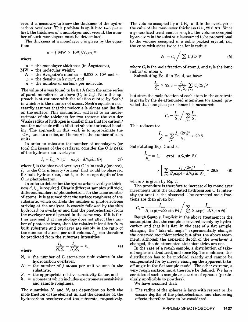
If it is assumed that the spheres are closely packed, then the approximation to a hemisphere is a reasonable one. If the spheres are not closely packed, then this ap- proximation breaks down. The extreme case is in square packing. In this case, if an additional sphere is considered below or above (cubic center packed), the area not con- forming to the hemisphere model is given in the shaded area in Fig. 2. This area is an additional 21% and is weighted towards low 0 or towards the flat sample cal- culation. Cubic packing of the additional sphere, on the other hand, would give the exact hemispherical model. Other models for the packing of the additional sphere(s) would lead to deviations from the hemispherical model, but would not represent more than an additional 21% of the area or 17 % of the whole.
E XPE R IME NT AL
Compounds were Analar grade, freshly ground in air and mounted on double-sided sellotape. The spectrom- eter was a Kratos ES200 operating in the fixed analyzer transmission (FAT) mode with a magnesium anode. The x-ray source-sample-analyzer angle was 90 ° .
Baseline subtraction was based on an algorithm as- suming inelastic scattering; 9 i.e., a straight baseline tan- gential to the noise on either side of the peak was first fitted. The points at which this straight baseline touched the noise defined the endpoints. The area above the straight baseline and the intensity difference between these endpoints were then determined. Thereafter a baseline was subtracted between the endpoints so that the amount subtracted in each channel was the intensity difference times the area to higher kinetic energy divided by the total area.
Intensities were then determined. The intensity for an isolated peak was simply the maximum of the baseline- subtracted, and five-point smoothed, data. Convoluted peaks were determined by peak synthesis with Gaussian peaks. 9 The software includes A1 K, 3,4 satellites where these are relevant, and allows spin-orbital doublets to be maintained at a constant energy difference and relative intensity.
The stoichiometries were derived from peak heights divided by the sensitivities of Wagner et al. 1° after ad- justment for the transmission function. The transmission function n for the PHI 550 used by Wagner et al. is E -°.°5, while the Kratos ES200 (this work) is E -°.ss. Peak area sensitivity factors, which are often ambiguous with re-
gard to exactly which peaks are included in their deter- mination, were not used.
In calculation of the IMFPs from Eq. 2, 46 eV was added to the observed kinetic energies to allow for the retardation in the FAT mode used in this study. The number of slices in the rough sample model was 10.
RESULTS AND DISCUSSION
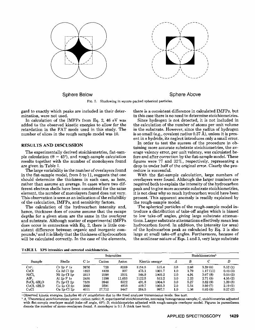
The experimentally derived stoichiometries, fiat-sam- ple calculation (0 = 45°), and rough-sample calculation results together with the number of monolayers found are given in Table I.
The large variability in the number of overlayers found in the flat-sample model, from 5 to 11, suggests that one should determine the thickness in each case, as here, rather than assume an average. In cases where two dif- ferent electron shells have been considered for the same element, the number of monolayers found does not vary. This observation is seen as an indication of the reliability of the calculation, IMFPs, and sensitivity factors.
The calculation of the hydrocarbon intensity and, hence, thickness does of course assume that the escape depths for a given atom are the same in the overlayer and substrate. Although scatter of experimental IMFPs does occur in connection with Eq. 2, there is little con- sistent difference between organic and inorganic com- pounds, 7 and it is likely that the thickness of hydrocarbon will be calculated correctly. In the case of the elements,
there is a consistent difference in calculated IMFPs, but in this case there is no need to determine stoichiometries.
Since hydrogen is not detected, it is not included in the calculation of the number of atoms per unit volume in the substrate. However, since the radius of hydrogen is so small (e.g., covalent radius 0.37/~), unless it is pres- ent in a hydride, its neglect introduces only a small error.
In order to test the success of the procedure in ob- taining more accurate substrate stoichiometries, the av- erage valency error, per unit valency, was calculated be- fore and after correction by the flat-sample model. These figures were 77 and 32%, respectively, representing a drop to under half of the original error. Clearly the pro- cedure is successful.
With the flat-sample calculation, large numbers of overlayers were found. Although the larger numbers are required both to explain the intensity of the hydrocarbon peak and to give more accurate substrate stoichiometries, it is not clear why so much hydrocarbon would have been present. This apparent anomaly is readily explained by the rough-sample model.
The spherical particles of the rough-sample model in- troduce a distribution of take-off angles which is biased to low take-off angles, giving large substrate attenua- tions. Larger substrate attenuations effectively mean less hydrocarbon found. In addition, the intensity (or area) of the hydrocarbon peak as calculated by Eq. 3 is also large at small take-off angles. Furthermore, because of the nonlinear nature of Eqs. 1 and 3, very large substrate
TABLE I. XPS intensities and corrected stoichiometries.
Intensities Stoichiometries b
Sample Shells C ls Cation Anion Kinetic energy ~ A B C D
a Observed kinetic energies. Includes 46 eV retardation due to the fixed analyzer transmission mode. See text. b A, Theoretical stoichiometries (anion : cation ratio); B, experimental stoichiometries, assuming homogeneous sample; C, stoichiometries adjusted
with fiat-sample overlayer model (take-off angle, 45°); D, stoichiometries adjusted with rough-sample overlayer model. Figures in parentheses denote the number of mono-overlayers found. A monolayer is 3.1/~ thick (see text).
APPLIED SPECTROSCOPY 1429
at tenuat ions and hydrocarbon intensit ies (or areas) are calculated at the low values of O, which are only par t ly compensa ted for as 0 rises. Indeed, in all cases, only two or three monolayers were found in the spherical rough- ness model, which contrasts with as many as eleven over- layers in the flat-sample model.
Another consequence of the nonlinear na ture of Eq. 1 is t ha t the der ived stoichiometries change between the flat-sample and rough-sample models. In the case where peaks are well separa ted in energy, the change is signif- icant. However, it mus t be emphasized tha t the " rough"- sample model here represents an ext reme case. In reality, even samples tha t topographical ly approximate the spherical model would have smaller particles between the spheres, be shadowed by adjacent particles, or be so small t ha t they approximate , in dimension, the photo- electron escape depths. All these effects reduce the weighting to low O, and a movement towards the flat- sample model would result.
The average valency error in the rough-sample model (57 % ) is not significantly be t te r than the un t rea ted data. I t can be seen by inspection of Table I tha t the rough- sample model usually introduces too much correct ion to the stoichiometries, consis tent with the hypothesis t ha t this model represents an ext reme case. The extent to which this happens varies between samples as a conse- quence of kinetic energy differences and the degree of roughness inheren t in the sample. If, however, the op- t imal s to ichiometry is arbi t rar i ly chosen between the two models, then the average valency error drops to 4 %.
I t is difficult to conceive of an exper iment to tes t the two models directly. A flat single crystal would introduce intensi ty/angle ambiguit ies due to diffraction of the pho- toelectrons, while a single macro-sized spherical sample may be so large tha t shadowing and a t tenua t ion of in- c ident x-rays would have to be considered so tha t each slice of the rough sample model would no longer have equal weight.
T he inclusion of the rough-sample calculation is there- fore potent ia l ly a t t ract ive since it can reduce the average valency error to a fract ion of its original value. Arbi t rary in terpola t ion between the two models is of no use in a real appl icat ion where the actual s toichiometries are not known. For this addi t ional ref inement to be of use, a me thod of defining the "degree of roughness" and hence a consis tent me thod for in terpolat ion between the two
models would be required. This in terpolat ion could well be based on exper imenta l results at different sample ori- entat ions, since the flat-sample model is sensitive to an- gle while the hemispherical model is invar iant with angle. Th e rough-sample model is, however, useful in tha t it does explain why the hydrocarbon peak is so large in powdered samples. In addit ion, it demonst ra tes the enor- mous s toichiometry changes tha t can be observed with powdered samples and well-separated photoelec t ron en- ergies. Its rout ine use would not only highlight these si tuations bu t also provide a good measure of how large the effect is likely to be.
C O N C L U S I O N
Th e flat sample overlayer model described yields more accurate surface stoichiometries than those derived from assumptions of complete sample homogeneity. The more sophist icated rough-sample model is capable of some fur- ther accuracy. Also the rough-sample model explains one reason for the larger measured levels of hydrocarbon contaminat ion in rough samples and highlights cases where large errors in s to ichiometry may occur.
ACKNOWLEDGMENTS We would like to thank D. J. Barnes and I. B. Parker for helpful
discussions.
1. Practical Surface Analysis by Auger X-ray Photoelectron Spec- troscopy, D. Briggs and M. P. Seah, Eds. (J. Wiley & Sons, Chieh- ester, 1983), p. 32.
2. W. A. Fraser, J. V. Florio, W. N. Delgass, and W. D. Robertson, Surf. Sci. 36, 661 (1973).
3. J. Brunner and H. Zogg, J. Electron Spectrosc. Relat. Phenom. 5, 911 (1974).
4. W. A. Frazer, J. V. Florio, W. N. Delgass, and W. D. Robertson, Rev. Sci. Instrum. 44, 1490 (1973).
5. M. Ebel, M. Schmid, H. Ebel, and A. Vogel, J. Electron Spectrosc. Relat. Phenom. 34, 313 (1984).
6. T. Reich and V. I. Nefedov, J. Electron Spectrosc. Relat. Phenom. 56, 33 (1991).
7. M. P. Seah and W. A. Deneh, Surf. Interface Anal, 1 (1), 2 (1979). 8. Lange's Handbook of Chemistry, J. A. Dean, Ed. (McGraw-Hill,
London, 1979), p. 3.120. 9. L. Griffiths, unpublished work.
10. C. D. Wagner, L. E. Davis, M. V. Zeller, J. A. Taylor, R. H. Ray- mond, and L. H. Gale, Surf. Interface Anal. 3 (5), 211 (1981).
11. M. P. Seah, M. E. Jones, and M. T. Anthony, Surf. Interface Anal. 6 (5), 242 (1984).