97
8 EUROPEAN COMMISSION THEME 8 Environment and energy WORKING PAPERS AND STUDIES Calculation of Indicators of Environmental Pressure caused by Transport 2003 EDITION Main report

8E U R O P E A NC O M M I S S I O N
THEME 8Environment and energyW
OR
KI
NG
P
AP
ER
S
AN
D
ST
UD
IE
S
Calculation of
Indicators of
EnvironmentalPressure caused by
Transport2
00
3 E
DIT
ION
Main report

A great deal of additional information on the European Union is available on the Internet.It can be accessed through the Europa server (http://europa.eu.int).
Luxembourg: Office for Official Publications of the European Communities, 2003
ISBN 92-894-5515-2ISBN 1725-0803
© European Communities, 2003
Europe Direct is a service to help you find answers to your questions about the European Union
New freephone number:
00 800 6 7 8 9 10 11

Table of Contents1 Introduction........................................................................................................................... 12 Summary................................................................................................................................ 33 Project overview.................................................................................................................... 4
3.1 Outline of the approach for road transport.......................................................................... 43.2 Outline of the approach for railways................................................................................... 53.3 Outline of the approach for maritime and inland shipping ................................................. 63.4 Outline of the approach for aviation ................................................................................... 7
3.4.1 Air traffic source data ................................................................................................. 73.4.2 Future emissions from IFR flights .............................................................................. 83.4.3 TRENDS/aviation methodology................................................................................. 8
3.5 Outline of the transport activity balance (TAB) module .................................................... 93.6 Outline of the noise study ................................................................................................. 11
4 Basecase scenario ................................................................................................................ 124.1 Overview........................................................................................................................... 124.2 Results per mode............................................................................................................... 12
4.2.1 Fleet data ................................................................................................................... 124.2.2 Vehicle emissions ..................................................................................................... 15
4.3 Results – Total .................................................................................................................. 264.3.1 Fleet data ................................................................................................................... 264.3.2 Vehicle emissions ..................................................................................................... 284.3.3 Contribution of each mode to the total EU15 emissions .......................................... 324.3.4 Emission factors........................................................................................................ 34
5 TRENDS - Auto Oil II comparison ................................................................................... 405.1 Activity data...................................................................................................................... 40
5.1.1 Road transport ........................................................................................................... 405.1.2 Maritime.................................................................................................................... 435.1.3 Railways.................................................................................................................... 46
5.2 Emission results ................................................................................................................ 496 Spatial disaggregation ........................................................................................................ 62
6.1 Road Transport.................................................................................................................. 626.1.1 HigHway emissions ................................................................................................... 626.1.2 Urban emissions........................................................................................................ 636.1.3 Rural emissions......................................................................................................... 636.1.4 Production of GIS maps............................................................................................ 63
6.2 Maritime shipping............................................................................................................. 676.3 Inland shipping.................................................................................................................. 696.4 Railways............................................................................................................................ 72
6.4.1 Attributing Intraplan-nodes to GISCO railway segments ......................................... 726.4.2 Attributing railway segments to NUTS regions........................................................ 76
7 Temporal disaggregation – road transport ...................................................................... 807.1 Data availability ................................................................................................................ 807.2 Methodology ..................................................................................................................... 807.3 Results............................................................................................................................... 81
8 Problems and Shortcomings of the present system.......................................................... 878.1 Road transport module...................................................................................................... 878.2 Railway, maritime and inland shipping modules.............................................................. 888.3 Air module ........................................................................................................................ 88
9 Future Developments.......................................................................................................... 89References.................................................................................................................................... 91

Appendix A: Seasonal distribution of CO2, NOx and PM emissions...................................... 92

Calculation of Indicators of Environmental Pressure Caused by Transport Main Report
1
1 INTRODUCTIONThe purpose of this study was to develop a system for calculating a range of environmentalpressures due to transport within a PC-based MS Access environment (TRansport andENvironment Database System - TRENDS). These environmental pressures include air emissionsfrom the four main transport modes, i.e. road, rail, ships and air. In addition, waste generation andnoise emissions from road transport were also addressed. Finally, the system provides an optionfor simple scenario analysis including vehicle dynamics (such as turnover and evolution) for allEU15 Member States.
The final aim of this study was to produce a range of transparent, consistent and comparableenvironmental pressure indicators caused by transport. These indicators were calculated directlyfrom the activity levels and reflect the potential change in the state of the environment, or the riskof specific environmental impacts which any changes in policy might have.
The TRENDS project was funded by the European Commission, Directorate-General forTransport and Energy and conceived and managed by Graham Lock in the Environment andSustainable Development Unit of Eurostat. The project was developed in the framework of acollaboration between members of the following institutes and organisations:
• Laboratory of Applied Thermodynamics, Aristotle University, Greece (LAT)
• Department of Energy Engineering, Denmark Technical University (DTU)
• AΨ -Consulting, Austria (PSIAMTK)
• INFRAS, Bern, Switzerland (INFRAS)
The Laboratory of Applied Thermodynamics (LAT), Aristotle University of Thessaloniki, Greece,was the co-ordinator of this study team and responsible for the administration of the project.
The project was completed in three phases, starting at 1997 as follows:
Phase I: December 1997 - December 1998 (EC contract: E1-B97-B2-7040-SIN 7674-SER) -Final Report of Phase I, December 1998
Phase II: March 1999 - March 2000 (EC contract: B99-B2704010-S72.7941-RE1 9930 -SER.STAT) - Final Report of Phase II, February 2000
Phase III: November 2000 - June 2002 (EC contract: B2000-B27040B-SI2.198159-SERARISTOTLE) – Main Report and Detailed reports, October 2002
This is volume 1 and the main report of the project. It summarises a series of detailed reports andprovides the basic conclusions of the work. The other detailed reports on which the main reportis based are the following:
2. Road Transport
3. Maritime and Inland Shipping
4. Railways
5. Aviation
6. Waste
7. Noise
8. Transport Activity Balance (TAB)
eurostat

Main Report Calculation of Indicators of Environmental Pressure Caused by Transport
2
Study TeamsLaboratory of Applied Thermodynamics – Aristotle University Thessaloniki (LAT/AUTh)
Zissis Samaras
Myrto Giannouli
Charis Kouridis
Evelina Tourlou
Theodoros Zachariadis
Aris Babatzimopoulos
Department of Energy Engineering, Denmark Technical University (DTU)
Spencer Sorenson
Aliki Georgakaki
Robert Coffey
AΨ -Consulting, Austria (PSIAMTK)
Manfred Kalivoda
Monika Kurdna
INFRAS, Bern, Switzerland (INFRAS)
Mario Keller
Peter deHaan
Roman Frick
René Zbinden
Philipp Wüthrich
eurostat

Calculation of Indicators of Environmental Pressure Caused by Transport Main Report
3
2 SUMMARYThe main parameters investigated in the framework of this project can be summarised as follows:
Air emissions from the following transport modes:
• Road (including all types of passenger and goods transport)
• Rail (including electrical trains, passenger and goods transport)
• Shipping (maritime and inland, passenger and goods transport)
• Air (national and international, passenger transport)
Pollutants covered: carbon monoxide; carbon dioxide; non-methane volatile organic compounds;methane; nitrous oxide; xxides of nitrogen; oxides of sulphur; lead, particulate matter (PM10)
• Waste production from road transport
• A feasibility study was conducted on noise emissions from road transport.
• Spatial resolution: The geographical distribution includes the EU15 Member States, as wellas cities, regions and different classes of infrastructure (e.g. urban and rural roads,motorways).
• Temporal resolution: Annual air emissions were disaggregated into seasonal emissions.
• Time span. The study provides time series of indicators for every year from 1970 to 2020.
• System dynamics, projections and forecasting: Extrapolations were conducted for futureyears, based on simple assumptions. Main emphasis was given on specific requirements forvehicle fleet dynamics (turnover, mean age, technology split etc.).
An important aspect of the project was to obtain feedback on data gaps, in particular where thesegaps had a significant influence on the reliability of the outputs.
The calculation system including the methodologies and related databases was transferred in acomputer model within a PC-based MS Access97 environment.
eurostat

Main Report Calculation of Indicators of Environmental Pressure Caused by Transport
4
3 PROJECT OVERVIEW
3.1 OUTLINE OF THE APPROACH FOR ROAD TRANSPORTThe road transport module developed in the framework of the TRENDS project produces bothanalytical and aggregated results for the EU15 countries and for a time-span of 50 years. Morespecifically, the road transport module calculates various transport-related parameters, such as theannual mileage, vehicle population, average age, vehicle emissions and fuel balance, for allvehicle categories considered by COPERT. Additionally, temporal and spatial disaggregation ofthe estimated vehicle emissions was conducted for the target year 1995.
For the estimation of air pollutant emissions from road transport a top down approach wasconsidered to be the most appropriate. Focus of the calculation was the annual air emissions of aCountry (each EU15 Member State). The time range was set from 1970 to 2020, with 1995defined as the base year for the calculations.
For air emissions and fuel consumption the COPERT III calculation module was applied. Afterannual air emissions were estimated on country basis, a spatial disaggregation module allocatedthe above annual air emissions to the different parts of the countries, using the initial COPERTestimates for urban, rural and highway split of the emissions for the different vehicle categories.At a final step, temporal disaggregation of vehicle emissions was conducted for each country,using appropriate patterns.
A detailed description of the methodological steps of the calculation for road transport follows:
Step 1: Creation of the appropriate databases for the calculation modules. All available Eurostatdatabases such as TRAINS and SIRENE were used in order to construct the appropriateinput for the calculations. In this respect, data concerning vehicle stocks, vehicle newregistrations, vehicle usage indicators (such as tonne-kilometres, passenger-kilometres,etc.) as well as fuel consumption for transport were used.
In addition to Eurostat, other sources of information were also incorporated (with mainemphasis on COPERT [1], TRAP [2] and MEET [3])) which provided additional datanot found in Eurostat. The information derived from these databases included usage datasuch as technology splits of vehicle fleets for certain years, annual mileage for differentvehicle categories, vehicle representative speeds, split of the annual mileage to differentroad classes, etc. Moreover, national data were also examined in order to fill gaps butalso to make comparisons and to calibrate the existing data.
Step 2: A system dynamics module was established in order to attain the following objectives:
(a) Extrapolation of the main vehicle categories into the future using data of the past.This was conducted using a sigmoid-type Gompertz function, which simulates theevolution of vehicle density. [3] The results of the extrapolation were combined withEurostat population forecasts per country in order to produce estimates of vehiclestocks per country.
(b) Simulation of the vehicle turnover for the main vehicle categories. This was achievedusing appropriate lifetime functions, which were developed by means of a Weibull-based function. The approach was calibrated on the basis of Eurostat data for theevolution of vehicle stock and new registrations.
(c) The above were supplemented with corresponding data on emissions technologyparameters which were introduced via a number of suitable implementation tables percountry, including simultaneous introduction of different legislation, scrappageschemes, etc.
eurostat

Calculation of Indicators of Environmental Pressure Caused by Transport Main Report
5
Step 3: The data resulting from the aforementioned processes were adapted in such a way as toproduce the input tables for the calculation of annual air emissions required by themethodology of COPERT. These input tables were produced for the entire calculationperiod, i.e. from 1970 to 2020. Especially as regards the future emission estimates, it wasnecessary to amend the legislation implementation tables with future estimates referringto the dates of introduction and to the effects of future legislation.
Step 4: Spatial disaggregation was performed using the basic annual estimates of COPERT andtheir split in urban, rural and highway modes, as follows:
• Highway emissions were directly allocated to the highway networks of the countries.To this aim, selected traffic counts from different types of highways were used inorder to produce appropriate traffic allocation patterns.
• Urban emissions were allocated to cities above a certain threshold (all settlementswith 20 000 or more inhabitants were considered as cities) of the different countries.The allocation was conducted using mainly the population data of the Eurostat/NewCronos database REGIO, but also complemented with other data, such as fuelconsumption and/or vehicle densities of the different countries, mainly in order toreflect differences between different regions of countries.
• The rural emissions produced by COPERT were allocated over the whole non-urbanarea of the EU15 countries, depending on the population density and regional GDP ofeach area.
Step 5: Temporal disaggregation: As Eurostat data on seasonal variation of transport activitieswere scarce, other sources of information were investigated. The only source of temporaldata discovered, was a project conducted in Austria [4], which contains a study of thetraffic load for different types of roads, depending on various time-related parameters.The monthly variations of the traffic load provided by this source were used in order toproduce the required seasonal variations of vehicle emissions.
Within the road transport module, a “waste from road transport” module was developed in orderto forecast the total waste production originating from end-of-life road transport vehicles.
The waste from road transport database produces “waste factors”. These waste factors representthe amount of waste for a given material or vehicle component as a function of activity, inanalogy to the emission factors for atmospheric pollutants. Waste factors were produced not onlyfor passenger cars, but also for light and heavy-duty vehicles as well as for motorcycles.
The waste factors within the database can be divided in two major categories:
• Waste produced during operation of road transport vehicles (in-use waste factors, expressedas a function of the veh-km travelled)
• Waste produced when the vehicle was finally taken from the road and shredded (so-calledend-of-life waste factors, expressed per scrapped vehicle).
All waste factors depend on the technology stage (EURO-I, -II, etc.) of the vehicle, in order toreflect the rapid change in technology and in the materials used over the last decades.
3.2 OUTLINE OF THE APPROACH FOR RAILWAYS
The purpose of the railway module was to establish a database that provides indicators forrailway transport in EU15 countries, between the years 1970 and 2020. In this study, only theenergy consumption of tractive movements and the consequent emissions of airborne pollutants
eurostat

Main Report Calculation of Indicators of Environmental Pressure Caused by Transport
6
were considered. Other activities such as maintaining infrastructure and vehicle stock, orenvironmental factors such as noise and vibration, were not examined.
The indicators produced were determined for both diesel and electric energy sources, as well asfor freight and passenger traffic. Results for energy consumption, CO2, SOx and NOx emissionswere plotted for all EU15 Member States for the year 1995.
In order to develop the railway database, traffic data provided by Eurostat were used, based onthe Eurostat New Cronos Rail Database, UIC and national sources.
A database was then constructed, which estimates emissions and energy consumption of railwaytransport from the year 1970 to the present day and provides projections up to the year 2020. Thedatabase was constructed in such a way that it may be updated or adapted with relative ease,should improved information become available.
A detailed database was also constructed for the base year 1995 by combining UIC data and dataprovided by the INTRAPLAN study [5]. The spatial resolution of the detailed database is on anetwork level. The resulting factors were attributed to the TEN railway corridors and to NUTSzones. The temporal range for the detailed database was limited to the year 1995, as this is theonly year for which data was available from the INTRAPLAN study.
With some correction in terms of the specific energy consumption of passenger trains and usingempirical results for freight trains, the energy consumption and emissions calculated in thedetailed database were estimated to within 30%, of published figures for national networks, withmost estimates lying within 20%.
Recommended measures to improve the estimation of indicators were given. These include theneed:
• to record the gross hauled tonne-kilometres of passenger and freight train movements at anetwork level
• to divide passenger traffic into categories on the basis of service
• to identify power sources in all traffic measurements
3.3 OUTLINE OF THE APPROACH FOR MARITIME AND INLANDSHIPPING
The TRENDS study of maritime shipping aimed to estimate the environmental pressures causedby the world’s commercial shipping fleet attending EU15 countries. According to the Lloydsregister [6] there are currently around 83 000 vessels operating in the world’s oceans with a totalgross tonnage of 491 million tonnes. The register excludes vessels under 100 GT as well asnaval, pleasure, unpowered craft or those restricted to canal, river or harbour service. It should benoted that the military fleet consists of around 20 000 vessels [7]. These are on average smallerthan their commercial counterparts and were not considered by this investigation.
Only shipping movements that involved contact with EU15 countries such as the delivery orreceipt of goods were considered. Ships passing through European waters without contact withthese countries were not considered by the study.
In terms of maritime transport, the structure and method of a detailed database was constructedwithin MS Access, which included all stages of the emissions and energy consumptioncalculations. The major technical assumptions were established and the necessary technicalfactors were incorporated within the database. This database was designed to operate on detailed
eurostat

Calculation of Indicators of Environmental Pressure Caused by Transport Main Report
7
statistical data provided by Eurostat. However, data was available only at port level, so a bottom-up approach was employed.
As the statistical data collection was not calibrated towards emission modelling, problems wereencountered in using the data successfully for that purpose. Since this bottom-up approach couldonly be conducted for a few years, aggregated data on a country level were used in order toprovide time series calculations through a second database.
The database for goods transport by inland waterways was completed within MS Access in termsof both structure and method. However, further work is required in order to support some of theassumed operational parameters such as loading factors and average speed. The nature of statisticsat country level does not allow for great detail in this database.
3.4 OUTLINE OF THE APPROACH FOR AVIATIONIncreasing numbers of flights and still unknown effects of exhaust gases on the high atmospherehave drawn attention on air traffic and its emissions. In Europe, many institutions work in thisarea, collecting traffic and emission data, creating emission inventories and assessing effects.That leads to some work done in parallel while using different databases and methodologies,which often lead to results that cannot be compared or matched.
For EU purposes, scenarios of future emissions need to be carried out centrally using a commonmethod and harmonised data sets. For that reason, Eurostat developed methods for estimatingemissions based on a single data set provided by Eurocontrol.
Eurocontrol is the European Organisation for Safety of Air Traffic. At the moment it has 28Member States, including the EU15 countries, with the exception of Finland. Eurocontrolprovides annual flight statistic data for a special area covered by its Member States. Although thedata does not include all the current EU Member States, it is indicative of the rate of changethroughout Europe.
3.4.1 AIR TRAFFIC SOURCE DATA
Air traffic in IFR (Instrument Flight Rules) flights is controlled by air traffic control services thatreport each flight to Eurocontrol.
Eurocontrol provided data on the profile flown and the aircraft type used for the 7 Mio. flightsthat were conducted in Eurocontrol area in 1997. This enabled the use of a bottom-up approachfor the estimation of emissions produced by aviation.
Detailed information on air traffic is only available for civil aviation and more specifically forIFR flights. For that reason, military aviation was not addressed in this study and IFR flightswere considered to be responsible for about 95% of air transport emissions.
Eurocontrol provides for the area covered by its Member States two detailed movementdatabanks:
• CRCO and
• CFMU
Records from these databases giving information on the flight profile were linked to emissiondata from aviation, provided by Eurostat.
Data from the AEA database (AEA technology) were also considered. These data cover the timeperiod 1975-1995 and are available for passenger-kilometres, tonne-kilometres, seat-kilometresand vehicle per kilometre for each country and year. These data also distinguish betweenpassenger and freight transport.
eurostat

Main Report Calculation of Indicators of Environmental Pressure Caused by Transport
8
3.4.2 FUTURE EMISSIONS FROM IFR FLIGHTS
In order to forecast the annual number of flights Eurocontrol adopts a method in which extremesand a baseline are analysed. Figure 3-1 is an adaptation of a figure that was published in airtraffic statistics and forecasts of Eurocontrol (June 1998).
EURO 88 - annual number of IFR flights (in thousands)
0
2000
4000
6000
8000
10000
12000
14000
16000
18000
1974
1977
1980
1983
1986
1989
1992
1995
1998
2001
2004
2007
2010
2013
2016
2019
Year
Num
ber o
f flig
hts
High ScenarioBaseline ScenarioLow Scenario
Figure 3-1: Air traffic forecast for the Eurocontrol area
Eurocontrol produced forecasts of air traffic up to and including 2015, based on three differentgrowth scenarios (high, low and baseline). According to these estimates, the number of flights inthe Eurocontrol area is expected to increase, from less than 6 million in 1998, to more than 10million in 2015 (see Figure 3-1).
The original chart produced by Eurocontrol, showed traffic statistics and forecast up to andincluding 2015. The remaining five-year forecast was extrapolated to give an indication of thetraffic until year 2020.
Emission scenarios are an important factor in the estimation of aircraft emission factors. Futureemissions from aviation depend on the balance between improvements in technology (producingmore efficient and less polluting aircrafts) and the growth in air transport. New and improvedtechnologies were briefly reviewed in this study and predictions of future levels of traffic wereexamined. On the basis of this information, a number of future scenarios for aircraft emissionswere produced [8].
3.4.3 TRENDS/AVIATION METHODOLOGY
In order to produce emission forecasts for the time period 2002-2020, the traffic increase rates of2002 – 2009 predicted by Eurocontrol (according to the baseline scenario) were extrapolateduntil the year 2020.
As mentioned in section 3.4.1, one source that publishes passenger-kilometres as well as tonne-kilometres is AEA. The passenger data provided by AEA were used to crosscheck theTRENDS/Aviation extrapolation. Unfortunately, this comparison revealed that the AEA dataseem to underestimate passenger-kilometres significantly (by a factor of 40-100).
eurostat

Calculation of Indicators of Environmental Pressure Caused by Transport Main Report
9
Since the discrepancy between freight data (tonne-kilometres) provided by Eurocontrol and therespective AEA data was considerable, only Eurocontrol data were used for the final calculationof air emissions. As a consequence, a significant deviation is expected between the emissionsproduced by TRENDS/Aviation and international statistical data.
The split between passenger and freight traffic was not possible due to the lack of freight data.As mentioned before, AEA passenger data were considered unsuitable and no other source offreight data was available for assessing the quality of AEA tonne-kilometre data. For that reason,freight data were not included in the TRENDS aviation database. As a result, all emissions fromaviation were allocated to passenger transport.
An MS Access computer tool was finally created, called AvioPOLL, which employs the MEETand AvioMEET methodologies in order to produce flight data. This tool enables the calculationof emissions for pairs of regions (departure region-destination region). The calculations areconducted quarterly, from quarter 1 in 1996, until the first quarter of 2002.
Moreover, a database was produced, which provides air emissions, including forecasts for thetime period 1970 to 2020. Emissions were generated per year according to the Eurocontrol splitinto:
• Short haul (SH)
• Medium haul (MH)
• Long haul western (LH)
For each region considered, emission data were also generated for movements, passenger-kilometres and vehicle-kilometres.
AvioPoll is a purely analysing tool, based on activity data provided by Eurocontrol for the years1996 till 2002. Combining actual (to be more precise actual flight plan) data with emissionfactors makes it possible to:
• Create an emission and fuel consumption inventory
• Analyse emissions and fuel consumption on a spatial disaggregated level
• Analyse emissions and fuel consumption for different aircraft types
• Create environmental indicators from emissions and passenger-kilometres and vehicle-kilometres
The activity data, which were incorporated into AvioPoll, represent aggregated number of flightsper origin/destination pairs per aircraft type groups. It was not foreseen to allow the user tochange any of this activity data in AvioPoll. Thus, it is not possible for example to change on agiven origin/destination pair actual aircraft type in order to assess the impact on environment. Itis also not possible to use AvioPoll in order to estimate air emissions for any years other than thetime period 1996-2002.
3.5 OUTLINE OF THE TRANSPORT ACTIVITY BALANCE (TAB)MODULE
A particular task within TRENDS deals with the “balance of the overall transport activity data”.This so called “transport activity balance” module (TAB) can be considered as a synthesis ofTRENDS since it allows to present the main data of all modes of TRENDS in a comparable way– in particular the traffic activity and the emissions associated with it. TAB also allows the userto perform a simple scenario analysis by assessing the effects of different assumptions about key
eurostat

Main Report Calculation of Indicators of Environmental Pressure Caused by Transport
10
factors like lower or higher overall transport activity evolution, modal shifts, different emissionstandards etc.
However, it was understood that this scenario analysis should be kept on a comparatively lowlevel of complexity. In particular, TAB was not designed to elaborate sophisticated socio-economic scenarios. It is rather the understanding that the “base case” (or “reference case”)scenario which was defined within the individual modules of TRENDS represents a commonlyaccepted development.
Varying some key factors leads to the creation of alternative scenarios. It is up to the user todefine “reasonable” variations of the assumptions. This should be possible for the time periodfrom 1970 up to 2020, (on a yearly basis) according to the time frame covered by TRENDS. Theappropriate level of spatial allocation is the country level or “EU15”, i.e. the aggregation of all 15countries of the European Union.
The results produced by TAB can be divided into two main categories: traffic activity andemission results. These results are given per country (and EU15 as a total) for all the yearsconsidered by TRENDS. A large number of options are available to the user for implementingthese results. Data produced by TAB can be displayed according to the traffic type(passenger/freight), according to the vehicle type and the vehicle technology. Figures 3-2 and 3-3present the different options provided for displaying the traffic activity and emission resultsrespectively.
Figure 3-2: TAB menu for displaying the traffic activity
Figure 3-3: TAB menu for displaying emission results
eurostat

Calculation of Indicators of Environmental Pressure Caused by Transport Main Report
11
3.6 OUTLINE OF THE NOISE STUDYNoise is the subjective description of sound. The perception of noise is dependent on thefrequencies, the sonar energy, its duration and regularity. Several methods have been developedto represent these variables with one single indicator. The most commonly used unit is dB(A).This unit therefore is taken as the indicator for assessing the disturbance of the population bynoise.
At very high noise levels (>120 dB(A)), noise can cause physical damage. The noise levelsreached by the various means of transport are, in general, much lower. Nevertheless, noise is asignificant source of annoyance and might lead to long-term psychological or physical damage.According to recent German studies about 2% of all heart attacks are caused by road noise. Inaddition, transport noise is a main source of disturbance of sleep and communications.
According to UBA [9], in Germany for example, 70% of the population perceive the noise fromroad traffic as annoyance, air traffic is second with 55%. This indicates that noise is indeed amajor concern.
In the framework of the TRENDS project, a feasibility study was conducted on noise emissionsdue to transport. The objective of the feasibility study was to evaluate ways and means of howthe disturbance by traffic noise can be measured and monitored. While a certain method for thecalculation of air pollutants exists, the assessment of noise and its monitoring creates new anddifferent types of questions since noise is a local problem. Therefore, in the case that noise istreated on an aggregated level, the classical treatment is likely to become obsolete and alternativeapproaches have to be investigated. This noise study was an attempt to sketch and evaluatedifferent possibilities to address the problems associated with noise.
There are various methods for measuring, calculating or monitoring noise and the annoyancecaused by noise. The methods can be classified in three main categories:
• Engineering approach
• Survey approach
• LCA (life cycle assessment) approach
Since the TRENDS project focuses in principle on vehicle emissions, it was consideredconsistent to apply the same approach for noise as well. Thus, noise emissions can be calculatedas noise indicators, using data produced by TRENDS whenever possible.
A very important element in the calculation of noise indicators is data availability. For that reason,it was suggested that the same data sets that were used for the development of the variousmodules should also be used for deriving the noise indicators. Finally, a methodology wasproposed for estimating noise emissions for three of the main transport modes: road, rail and air.Noise emissions from shipping were considered to be negligible.
eurostat

Main Report Calculation of Indicators of Environmental Pressure Caused by Transport
12
4 BASECASE SCENARIO
4.1 OVERVIEWAs mentioned in section 3.5, the “Transport Activity Balance” (TAB) module allows a simplescenario analysis by assessing the effects of different assumptions about key factors like lower orhigher overall transport activity evolution, modal shifts or changes in technology mixes (e.g.petrol / diesel) etc.
Within the TAB module the user has the ability to change different parameters concerning thetraffic activity within TAB. The software then calculates the traffic activity and emission resultson different levels of detail (e.g. per vehicle class, per mode, or total emissions).
The data incorporated in TAB were produced from the different mode-specific modules. Thesemodules provided traffic activity data as well as emissions for the time period 1970-2020. Thesedata represent the reference or basecase scenario.
The traffic activity data included in the reference scenario were based on statistical resultsprovided by Eurostat and other sources. In order to obtain complete sets of timeseries, availabledata were either extrapolated to missing years or kept constant over the time period 1970-2020.
An example of this is the share of diesel, gasoline and LPG vehicles in road transport. In order toevaluate this share, statistical data provided by Eurostat were used, (available only until the years1995-97) referring to both new registrations and total fleet. From these data, values of the vehiclesplit were obtained for all EU15 countries, which were kept constant over the entire calculationperiod. This stability in diesel/gasoline/LPG shares may not reflect the actual situation in Europe.For example, some countries (e.g. France, Germany, Austria) recently exhibited a tendencytowards increasing diesel share. These tendencies were not considered in the basecase scenario.In the future, additional scenarios can be created in order to account for such effects.
The following sections provide examples of traffic activity and emission results producedaccording to the basecase (reference) scenario. All data were obtained from the TAB moduleversion 04h.
4.2 RESULTS PER MODE
4.2.1 FLEET DATA
Figures 4-1 to 4-5 show the annual vehicle-kilometres predicted by each mode (i.e. aviation,maritime, railway, road transport and inland shipping) for all EU15 countries. These resultsdistinguish between freight and passenger vehicle-kilometres for the time period 1970-2020.From these figures it can be observed that all transport modes exhibit an increase in vehicle-kilometres, as expected.
eurostat

Calculation of Indicators of Environmental Pressure Caused by Transport Main Report
13
EU 15 Air Veh Km
0
5,000
10,000
15,000
20,000
25,000
1970 1975 1980 1985 1990 1995 2000 2005 2010 2015 2020
Year
mio
Veh
Km
PassengerFreight
Figure 4-1: EU15 vehicle-kilometres for passenger and freight transport predicted by the airmodule from 1970 to 2020
EU 15 Rail Veh Km
0
500
1,000
1,500
2,000
2,500
3,000
3,500
4,000
1970 1975 1980 1985 1990 1995 2000 2005 2010 2015 2020
Year
mio
Veh
Km
PassengerFreight
Figure 4-2: EU15 vehicle-kilometres for passenger and freight transport predicted by the railwaymodule from 1970 to 2020
eurostat

Main Report Calculation of Indicators of Environmental Pressure Caused by Transport
14
EU 15 Maritime Veh Km
0
200
400
600
800
1,000
1,200
1,400
1,600
1,800
2,000
1970 1975 1980 1985 1990 1995 2000 2005 2010 2015 2020
Year
mio
Veh
Km
PassengerFreight
Figure 4-3: EU15 vehicle-kilometres for passenger and freight transport predicted by themaritime shipping module from 1970 to 2020
EU 15 Road Veh Km
0
500,000
1,000,000
1,500,000
2,000,000
2,500,000
3,000,000
3,500,000
4,000,000
4,500,000
1970 1975 1980 1985 1990 1995 2000 2005 2010 2015 2020
Year
mio
Veh
Km
PassengerFreight
Figure 4-4: EU15 vehicle-kilometres for passenger and freight transport predicted by the roadtransport module from 1970 to 2020
eurostat

Calculation of Indicators of Environmental Pressure Caused by Transport Main Report
15
EU 15 Inland Veh Km
0
50
100
150
200
250
1970 1975 1980 1985 1990 1995 2000 2005 2010 2015 2020
Year
mio
Veh
Km
PassengerFreight
Figure 4-5: EU15 vehicle-kilometres for passenger and freight transport predicted by the inlandshipping transport module from 1970 to 2020
4.2.2 VEHICLE EMISSIONS
Figures 4-6 to 4-25 represent the annual CO, NOx, HC and CO2 emissions produced by eachmode for all EU15 countries. The results are presented in terms of passenger and freightemissions for the time period 1970-2020.
From these figures the following observations can be made:
• Emissions from air transport increase steadily throughout the entire calculation period.However, an anomaly can be detected in the curve between the years 1996 and 2001. This isdue to the fact that actual movement data were used for the calculation of emissions duringthat period, while the emissions produced for the remaining years are mostly the result ofextrapolations.
• Rail emissions (with the exception of CO2) present a slight decrease from 1970 to 2020, eventhough the respective vehicle-kilometres increase during this period (cf. Figure 4-2). Thiseffect is probably due to the increasing use of electric trains, which do not produce airemissions but contribute to the overall energy consumption.
• Maritime emissions present a considerable increase, as expected, since maritime vehicle-kilometres also increase significantly between the years 1970 and 2020. (cf. Figure 4-3)
• Road transport emissions rise considerably until the years 1985-1990. After this time,emissions from road transport drop rapidly until they reach very low levels. This is due to theintroduction of improved technologies (e.g. catalysts) and to the administration of morestringent legislation measures. The exception to this tendency is CO2 emissions, whichincrease steadily. This is a direct consequence of the increasing road activity observed inEU15 countries (cf. Figure 4-4)
• Emissions produced by inland shipping present a slight upward trend without any significantvariations, in agreement with the respective vehicle-kilometre results (Figure 4-5)
eurostat

Main Report Calculation of Indicators of Environmental Pressure Caused by Transport
16
EU15 CO Air Emissions
0
20,000
40,000
60,000
80,000
100,000
120,000
140,000
160,000
180,000
1970 1975 1980 1985 1990 1995 2000 2005 2010 2015 2020
Year
Tons Passenger
Freight
Figure 4-6: CO emissions [t] for EU15 countries produced by passenger and freight air transportfrom 1970 to 2020
EU15 CO Rail Emissions
0
5,000
10,000
15,000
20,000
25,000
30,000
1970 1975 1980 1985 1990 1995 2000 2005 2010 2015 2020
Year
Tons Passenger
Freight
Figure 4-7: CO emissions [t] for EU15 countries produced by passenger and freight railwaytransport from 1970 to 2020
eurostat

Calculation of Indicators of Environmental Pressure Caused by Transport Main Report
17
EU15 CO Maritime Emissions
0
100,000
200,000
300,000
400,000
500,000
600,000
1970 1975 1980 1985 1990 1995 2000 2005 2010 2015 2020Year
Tons Passenger
Freight
Figure 4-8: CO emissions [t] for EU15 countries produced by passenger and freight maritimeshipping from 1970 to 2020
EU15 CO Road Emissions
0
5,000,000
10,000,000
15,000,000
20,000,000
25,000,000
30,000,000
35,000,000
40,000,000
45,000,000
50,000,000
1970 1975 1980 1985 1990 1995 2000 2005 2010 2015 2020Year
Tons Passenger
Freight
Figure 4-9: CO emissions [t] for EU15 countries produced by passenger and freight roadtransport from 1970 to 2020
eurostat

Main Report Calculation of Indicators of Environmental Pressure Caused by Transport
18
EU15 CO Inland Emissions
0
500
1,000
1,500
2,000
2,500
3,000
3,500
4,000
4,500
1970 1975 1980 1985 1990 1995 2000 2005 2010 2015 2020Year
Tons Passenger
Freight
Figure 4-10: CO emissions [t] for EU15 countries produced by passenger and freight inlandshipping from 1970 to 2020
EU15 NOx Air Emissions
0
100,000
200,000
300,000
400,000
500,000
600,000
700,000
800,000
900,000
1,000,000
1970 1975 1980 1985 1990 1995 2000 2005 2010 2015 2020
Year
Tons Passenger
Freight
Figure 4-11: NOx emissions [t] for EU15 countries produced by passenger and freight airtransport from 1970 to 2020
eurostat

Calculation of Indicators of Environmental Pressure Caused by Transport Main Report
19
EU15 NOx Rail Emissions
0
20,000
40,000
60,000
80,000
100,000
120,000
140,000
160,000
180,000
1970 1975 1980 1985 1990 1995 2000 2005 2010 2015 2020
Year
Tons Passenger
Freight
Figure 4-12: NOx emissions [t] for EU15 countries produced by passenger and freight railtransport from 1970 to 2020
EU15 NOx Maritime Emissions
0
1,000,000
2,000,000
3,000,000
4,000,000
5,000,000
6,000,000
1970 1975 1980 1985 1990 1995 2000 2005 2010 2015 2020Year
Tons Passenger
Freight
Figure 4-13: NOx emissions [t] for EU15 countries produced by passenger and freight maritimeshipping from 1970 to 2020
eurostat

Main Report Calculation of Indicators of Environmental Pressure Caused by Transport
20
EU15 NOx Road Emissions
0
1,000,000
2,000,000
3,000,000
4,000,000
5,000,000
6,000,000
7,000,000
1970 1975 1980 1985 1990 1995 2000 2005 2010 2015 2020Year
Tons Passenger
Freight
Figure 4-14: NOx emissions [t] for EU15 countries produced by passenger and freight roadtransport from 1970 to 2020
EU15 NOx Inland Emissions
0
10,000
20,000
30,000
40,000
50,000
60,000
70,000
80,000
90,000
1970 1975 1980 1985 1990 1995 2000 2005 2010 2015 2020Year
Tons Passenger
Freight
Figure 4-15: NOx emissions [t] for EU15 countries produced by passenger and freight inlandshipping from 1970 to 2020
eurostat

Calculation of Indicators of Environmental Pressure Caused by Transport Main Report
21
EU15 HC Air Emissions
0
10,000
20,000
30,000
40,000
50,000
60,000
70,000
80,000
1970 1975 1980 1985 1990 1995 2000 2005 2010 2015 2020
Year
Tons Passenger
Freight
Figure 4-16: HC emissions [t] for EU15 countries produced by passenger and freight airtransport from 1970 to 2020
EU15 HC Rail Emissions
0
1,000
2,000
3,000
4,000
5,000
6,000
7,000
8,000
1970 1975 1980 1985 1990 1995 2000 2005 2010 2015 2020
Year
Tons Passenger
Freight
Figure 4-17: HC emissions [t] for EU15 countries produced by passenger and freight railtransport from 1970 to 2020
eurostat

Main Report Calculation of Indicators of Environmental Pressure Caused by Transport
22
EU15 HC Maritime Emissions
0
20,000
40,000
60,000
80,000
100,000
120,000
140,000
160,000
180,000
1970 1975 1980 1985 1990 1995 2000 2005 2010 2015 2020Year
Tons Passenger
Freight
Figure 4-18: HC emissions [t] for EU15 countries produced by passenger and freight maritimeshipping from 1970 to 2020
EU15 HC Road Emissions
0
1,000,000
2,000,000
3,000,000
4,000,000
5,000,000
6,000,000
7,000,000
1970 1975 1980 1985 1990 1995 2000 2005 2010 2015 2020Year
Tons Passenger
Freight
Figure 4-19: HC emissions [t] for EU15 countries produced by passenger and freight roadtransport from 1970 to 2020
eurostat

Calculation of Indicators of Environmental Pressure Caused by Transport Main Report
23
EU15 HC Inland Emissions
0
500
1,000
1,500
2,000
2,500
3,000
3,500
4,000
4,500
1970 1975 1980 1985 1990 1995 2000 2005 2010 2015 2020Year
Tons Passenger
Freight
Figure 4-20: HC emissions [t] for EU15 countries produced by passenger and freight inlandshipping from 1970 to 2020
EU15 CO2 Air Emissions
0
50,000,000
100,000,000
150,000,000
200,000,000
250,000,000
300,000,000
1970 1975 1980 1985 1990 1995 2000 2005 2010 2015 2020
Year
Tons Passenger
Freight
Figure 4-21: CO2 emissions [t] for EU15 countries produced by passenger and freight airtransport from 1970 to 2020
eurostat

Main Report Calculation of Indicators of Environmental Pressure Caused by Transport
24
EU15 CO2 Rail Emissions
0
5,000,000
10,000,000
15,000,000
20,000,000
25,000,000
30,000,000
1970 1975 1980 1985 1990 1995 2000 2005 2010 2015 2020
Year
Tons Passenger
Freight
Figure 4-22: CO2 emissions [t] for EU15 countries produced by passenger and freight railtransport from 1970 to 2020
EU15 CO2 Maritime Emissions
0
50,000,000
100,000,000
150,000,000
200,000,000
250,000,000
1970 1975 1980 1985 1990 1995 2000 2005 2010 2015 2020Year
Tons Passenger
Freight
Figure 4-23: CO2 emissions [t] for EU15 countries produced by passenger and freight maritimeshipping from 1970 to 2020
eurostat

Calculation of Indicators of Environmental Pressure Caused by Transport Main Report
25
EU15 CO2 Road Emissions
0
200,000,000
400,000,000
600,000,000
800,000,000
1,000,000,000
1,200,000,000
1970 1975 1980 1985 1990 1995 2000 2005 2010 2015 2020Year
Tons Passenger
Freight
Figure 4-24: CO2 emissions [t] for EU15 countries produced by passenger and freight roadtransport from 1970 to 2020
EU15 CO2 Inland Emissions
0
500,000
1,000,000
1,500,000
2,000,000
2,500,000
3,000,000
3,500,000
4,000,000
4,500,000
1970 1975 1980 1985 1990 1995 2000 2005 2010 2015 2020Year
Tons Passenger
Freight
Figure 4-25: CO2 emissions [t] for EU15 countries produced by passenger and freight inlandshipping from 1970 to 2020
eurostat

Main Report Calculation of Indicators of Environmental Pressure Caused by Transport
26
4.3 RESULTS – TOTAL
4.3.1 FLEET DATA
Figures 4-26 and 4-27 present the annual vehicle-kilometres produced by each mode during thetime period 1970-2020, for passenger and freight transport respectively. From these figures it isclear that vehicle-kilometre road transport values are considerably higher than the predictedvehicle-kilometres for all other modes, mainly due to the large number of road transport vehiclesin the EU.
Figures 4-28 and 4-29 show the annual passenger-kilometres and tonne-kilometres respectively,produced by each mode during the time period 1970-2020. From Figure 4-28 it can be observedthat the predominant means of passenger transport are air and road, while according to Figure 4-29, the transportation of goods is mainly conducted by sea and in a smaller degree by road.
EU15 Veh Km from Passenger Transport
0
500,000
1,000,000
1,500,000
2,000,000
2,500,000
3,000,000
3,500,000
1970 1975 1980 1985 1990 1995 2000 2005 2010 2015 2020
Year
mio
Veh
Km Air
MaritimeInlandRoadRail
Figure 4-26: Annual vehicle-kilometres produced by passenger transport for all EU15 countriesfrom 1970 to 2020
eurostat

Calculation of Indicators of Environmental Pressure Caused by Transport Main Report
27
EU15 Veh Km from Freight Transport
0
200,000
400,000
600,000
800,000
1,000,000
1,200,000
1970 1975 1980 1985 1990 1995 2000 2005 2010 2015 2020
Year
mio
Veh
Km Air
MaritimeInlandRoadRail
Figure 4-27: Annual vehicle-kilometres produced by freight transport for all EU15 countriesfrom 1970 to 2020
EU15 Pas Km
0
1,000,000
2,000,000
3,000,000
4,000,000
5,000,000
6,000,000
7,000,000
8,000,000
9,000,000
1970 1975 1980 1985 1990 1995 2000 2005 2010 2015 2020
Year
mio
Pas
Km Air
MaritimeInlandRoadRail
Figure 4-28: Annual passenger-kilometres predicted by TRENDS for all EU15 countries from1970 to 2020
eurostat

Main Report Calculation of Indicators of Environmental Pressure Caused by Transport
28
EU15 Ton Km
0
5,000,000
10,000,000
15,000,000
20,000,000
25,000,000
1970 1975 1980 1985 1990 1995 2000 2005 2010 2015 2020
Year
mio
Ton
Km Air
MaritimeInlandRoadRail
Figure 4-29: Annual tonne-kilometres predicted by TRENDS for all EU15 countries from 1970to 2020
4.3.2 VEHICLE EMISSIONS
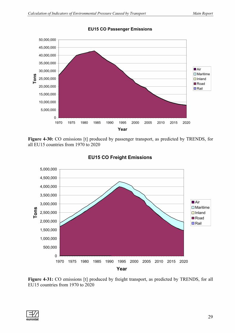
Figures 4-30 through 4-37 present the annual CO, NOx, HC and CO2 emissions produced bypassenger and freight transport for all modes, during the time period 1970-2020. From thesefigures it can be seen that emissions from passenger transport are mostly produced from the roadand air modes, while emissions from the transport of goods are mainly produced by road andmaritime. These results are in agreement with the passenger-kilometre and tonne-kilometre datapresented in the previous section.
eurostat
Calculation of Indicators of Environmental Pressure Caused by Transport Main Report
29
EU15 CO Passenger Emissions
0
5,000,000
10,000,000
15,000,000
20,000,000
25,000,000
30,000,000
35,000,000
40,000,000
45,000,000
50,000,000
1970 1975 1980 1985 1990 1995 2000 2005 2010 2015 2020
Year
Tons
AirMaritimeInlandRoadRail
Figure 4-30: CO emissions [t] produced by passenger transport, as predicted by TRENDS, forall EU15 countries from 1970 to 2020
EU15 CO Freight Emissions
0
500,000
1,000,000
1,500,000
2,000,000
2,500,000
3,000,000
3,500,000
4,000,000
4,500,000
5,000,000
1970 1975 1980 1985 1990 1995 2000 2005 2010 2015 2020
Year
Tons
AirMaritimeInlandRoadRail
Figure 4-31: CO emissions [t] produced by freight transport, as predicted by TRENDS, for allEU15 countries from 1970 to 2020
eurostat

Main Report Calculation of Indicators of Environmental Pressure Caused by Transport
30
EU15 NOx Passenger Emissions
0
500,000
1,000,000
1,500,000
2,000,000
2,500,000
3,000,000
3,500,000
4,000,000
4,500,000
5,000,000
1970 1975 1980 1985 1990 1995 2000 2005 2010 2015 2020
Year
Tons
AirMaritimeInlandRoadRail
Figure 4-32: NOx emissions [t] produced by passenger transport, as predicted by TRENDS, forall EU15 countries from 1970 to 2020
EU15 NOx Freight Emissions
0
1,000,000
2,000,000
3,000,000
4,000,000
5,000,000
6,000,000
7,000,000
8,000,000
1970 1975 1980 1985 1990 1995 2000 2005 2010 2015 2020
Year
Tons
MaritimeInlandRoadRail
Figure 4-33: NOx emissions [t] produced by freight transport, as predicted by TRENDS, for allEU15 countries from 1970 to 2020
eurostat

Calculation of Indicators of Environmental Pressure Caused by Transport Main Report
31
EU15 HC Passenger Emissions
0
1,000,000
2,000,000
3,000,000
4,000,000
5,000,000
6,000,000
1970 1975 1980 1985 1990 1995 2000 2005 2010 2015 2020
Year
Tons
AirMaritimeInlandRoadRail
Figure 4-34: HC emissions [t] produced by passenger transport, as predicted by TRENDS, forall EU15 countries from 1970 to 2020
EU15 HC Freight Emissions
0
100,000
200,000
300,000
400,000
500,000
600,000
700,000
800,000
900,000
1,000,000
1970 1975 1980 1985 1990 1995 2000 2005 2010 2015 2020
Year
Tons
AirMaritimeInlandRoadRail
Figure 4-35: HC emissions [t] produced by freight transport, as predicted by TRENDS, for allEU15 countries from 1970 to 2020
eurostat

Main Report Calculation of Indicators of Environmental Pressure Caused by Transport
32
EU15 CO2 Passenger Emissions
0
100,000,000
200,000,000
300,000,000
400,000,000
500,000,000
600,000,000
700,000,000
800,000,000
900,000,000
1,000,000,000
1970 1975 1980 1985 1990 1995 2000 2005 2010 2015 2020
Year
Tons
AirMaritimeInlandRoadRail
Figure 4-36: CO2 emissions [t] produced by passenger transport, as predicted by TRENDS, forall EU15 countries from 1970 to 2020
EU15 CO2 Freight Emissions
0
100,000,000
200,000,000
300,000,000
400,000,000
500,000,000
600,000,000
700,000,000
800,000,000
1970 1975 1980 1985 1990 1995 2000 2005 2010 2015 2020
Year
Tons
AirMaritimeInlandRoadRail
Figure 4-37: CO2 emissions [t] produced by freight transport, as predicted by TRENDS, for allEU15 countries from 1970 to 2020
4.3.3 CONTRIBUTION OF EACH MODE TO THE TOTAL EU15 EMISSIONS
Figures 4-38 to 4-41 exhibit the contribution of each mode to the total CO, NOx, HC and CO2emissions produced in the EU during the year 1995. From these figures it can be observed that
eurostat

Calculation of Indicators of Environmental Pressure Caused by Transport Main Report
33
road transport is the main source of CO and HC emissions. Road transport is also responsible forthe greatest part of NOx and CO2 emissions. However, air and maritime emissions also present asignificant contribution towards the production of NOx and CO2 emissions in the EU.
EU15 1995 CO Emissions [Tons]
RailRoadInlandMaritimeAir
Figure 4-38: Comparison between the CO emissions [t] predicted by all modes for the year 1995for EU15 countries
EU15 1995 NOx Emissions [Tons]
RailRoadInlandMaritimeAir
Figure 4-39: Comparison between the NOx emissions [t] predicted by all modes for the year1995 for EU15 countries
eurostat

Main Report Calculation of Indicators of Environmental Pressure Caused by Transport
34
EU15 1995 HC Emissions [Tons]
RailRoadInlandMaritimeAir
Figure 4-40: Comparison between the HC emissions [t] predicted by all modes for the year 1995for EU15 countries
EU15 1995 CO2 Emissions [Tons]
RailRoadInlandMaritimeAir
Figure 4-41: Comparison between the CO2 emissions [t] predicted by all modes for the year1995 for EU15 countries
4.3.4 EMISSION FACTORS
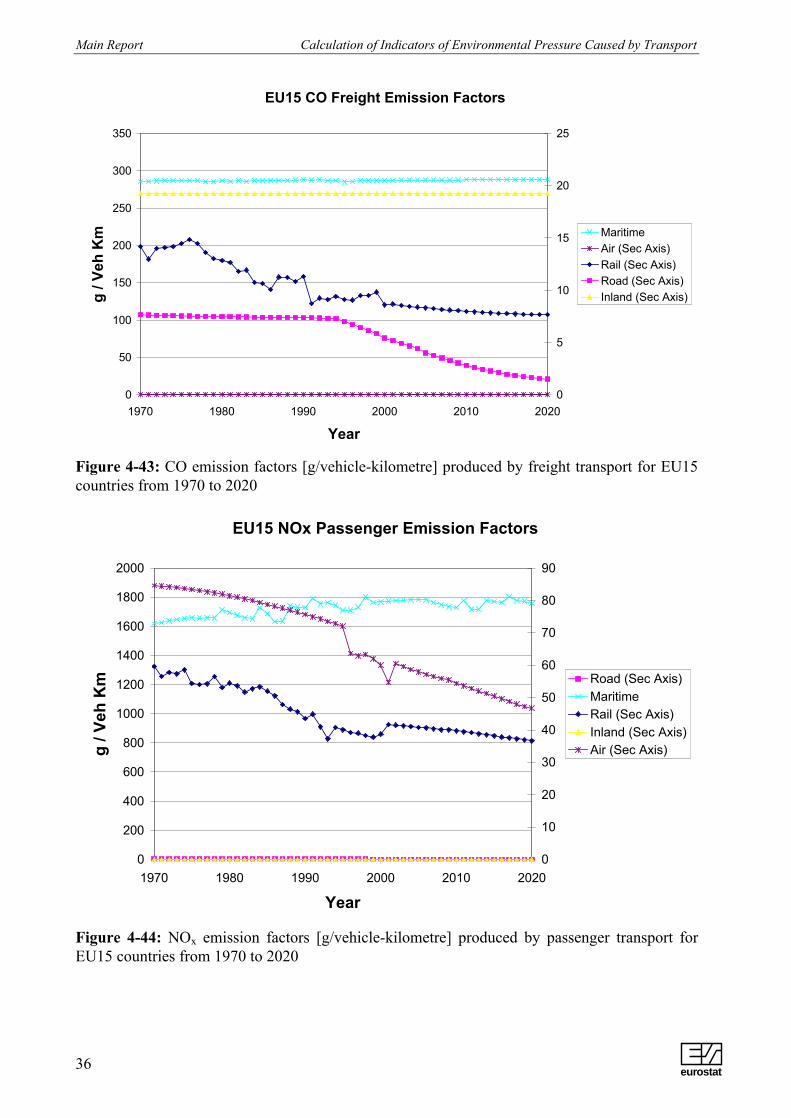
Figures 4-42 to 4-50 present annual emission factors (g/vehicle-kilometre) produced by allmodes for passenger and freight transport from 1970 to 2020.
eurostat

Calculation of Indicators of Environmental Pressure Caused by Transport Main Report
35
From these figures it can be observed that emission factors (g/vehicle-kilometre) produced byroad transport decrease considerably over the years. This tendency is consistent with theobserved decrease in annual road transport emissions (see section 4.2.2) as well as with theincrease of road transport vehicle-kilometres (cf. Figure 4-4).
EU15 CO Passenger Emission Factors
0
20
40
60
80
100
120
140
160
180
1970 1980 1990 2000 2010 2020
Year
g / V
eh K
m
0
5
10
15
20
25
30
35
Inland (Sec Axis)MaritimeRail (Sec Axis)Road (Sec Axis)Air (Sec Axis)
Figure 4-42: CO emission factors [g/vehicle-kilometre] produced by passenger transport forEU15 countries from 1970 to 2020
eurostat
Main Report Calculation of Indicators of Environmental Pressure Caused by Transport
36
EU15 CO Freight Emission Factors
0
50
100
150
200
250
300
350
1970 1980 1990 2000 2010 2020
Year
g / V
eh K
m
0
5
10
15
20
25
MaritimeAir (Sec Axis)Rail (Sec Axis)Road (Sec Axis)Inland (Sec Axis)
Figure 4-43: CO emission factors [g/vehicle-kilometre] produced by freight transport for EU15countries from 1970 to 2020
EU15 NOx Passenger Emission Factors
0
200
400
600
800
1000
1200
1400
1600
1800
2000
1970 1980 1990 2000 2010 2020
Year
g / V
eh K
m
0
10
20
30
40
50
60
70
80
90
Road (Sec Axis)MaritimeRail (Sec Axis)Inland (Sec Axis)Air (Sec Axis)
Figure 4-44: NOx emission factors [g/vehicle-kilometre] produced by passenger transport forEU15 countries from 1970 to 2020
eurostat

Calculation of Indicators of Environmental Pressure Caused by Transport Main Report
37
EU15 NOx Passenger Emission Factors
0
10
20
30
40
50
60
70
80
90
1970 1980 1990 2000 2010 2020
Year
g / V
eh K
m
0
0.5
1
1.5
2
2.5
Rail Air Road (Sec Axis)Inland (Sec Axis)
Figure 4-45: Detail of Figure 5-44, showing NOx emission factors [g/vehicle-kilometre]produced by passenger transport for EU15 countries from 1970 to 2020
EU15 NOx Freight Emission Factors
0
500
1000
1500
2000
2500
3000
3500
1970 1980 1990 2000 2010 2020
Year
g / V
eh K
m
0
10
20
30
40
50
60
70
80
90
InlandMaritimeAirRail (Sec Axis)Road (Sec Axis)
Figure 4-46: NOx emission factors [g/vehicle-kilometre] produced by freight transport for EU15countries from 1970 to 2020
eurostat

Main Report Calculation of Indicators of Environmental Pressure Caused by Transport
38
EU15 HC Passenger Emission Factors
0
10
20
30
40
50
60
1970 1980 1990 2000 2010 2020
Year
g / V
eh K
m
0
1
2
3
4
5
6
7
8
9
10
Inland (Sec Axis)MaritimeRail (Sec Axis)Road (Sec Axis)Air (Sec Axis)
Figure 4-47: HC emission factors [g/vehicle-kilometre] produced by passenger transport forEU15 countries from 1970 to 2020
EU15 HC Freight Emission Factors
0
10
20
30
40
50
60
70
80
90
100
1970 1980 1990 2000 2010 2020
Year
g / V
eh K
m
0
5
10
15
20
25
MaritimeAir (Sec Axis)Rail (Sec Axis)Road (Sec Axis)Inland (Sec Axis)
Figure 4-48: HC emission factors [g/vehicle-kilometre] produced by freight transport for EU15countries from 1970 to 2020
eurostat

Calculation of Indicators of Environmental Pressure Caused by Transport Main Report
39
EU15 CO2 Passenger Emission Factors
0
10000
20000
30000
40000
50000
60000
70000
80000
1970 1980 1990 2000 2010 2020
Year
g / V
eh K
m
205
210
215
220
225
230
235
RailInlandMaritimeAirRoad (Sec Axis)
Figure 4-49: CO2 emission factors [g/vehicle-kilometre] produced by passenger transport forEU15 countries from 1970 to 2020
EU15 CO2 Freight Emission Factors
0
20000
40000
60000
80000
100000
120000
140000
1970 1980 1990 2000 2010 2020
Year
g / V
eh K
m
462
464
466
468
470
472
474
476
478
RailInlandMaritimeAirRoad (Sec Axis)
Figure 4-50: CO2 emission factors [g/vehicle-kilometre] produced by freight transport for EU15countries from 1970 to 2020
eurostat

Main Report Calculation of Indicators of Environmental Pressure Caused by Transport
40
5 TRENDS - AUTO OIL II COMPARISONA comparison was conducted between TRENDS estimates and data produced by the Auto Oil IIstudy (basecase scenario) [10] in order to assess the quality of traffic activity and emission resultspredicted by TRENDS.
The Auto Oil II study provides data for nine EU countries. From these countries, the followingcountries were considered for this comparison: Finland, Germany, Italy, Netherlands and UK.The Auto Oil II database contains traffic activity and air emission data for the years 1990-2020.For that reason, the time period 1990-2020 was selected for this comparison.
Emission results from the Auto Oil II study, are only available for air emissions produced by roadtransport. However, activity data are available for road transport, as well as for waterways andtrains.
5.1 ACTIVITY DATA
5.1.1 ROAD TRANSPORT
Figures 5-1 to 5-5 represent a comparison between TRENDS and Auto Oil II (AOII) vehicle-kilometres produced by passenger road transport for the aforementioned countries. From thesefigures it can be observed that in general, there is a satisfactory agreement between TRENDS andAOII traffic activity data for road transport. The difference between the results produced by thetwo sources is as low as 3-5% in some countries (cf. Figure 5-3). Large deviations can beobserved mostly in future years (2015-2020) and in some cases they reach values as high as 30-40% (cf. Figure 5-4)
Comparison of road veh km produced by passenger transport for Finland
0
10,000
20,000
30,000
40,000
50,000
60,000
70,000
1990
1992
1994
1996
1998
2000
2002
2004
2006
2008
2010
2012
2014
2016
2018
2020
Year
Ann
ual v
eh k
m (m
illio
n)
TRENDS
Auto Oil II
Figure 5-1: Annual road vehicle-kilometres produced by passenger transport for Finland
eurostat

Calculation of Indicators of Environmental Pressure Caused by Transport Main Report
41
Comparison of road veh km produced by passenger transport for Germany
0
100,000
200,000
300,000
400,000
500,000
600,000
700,000
800,000
1990
1992
1994
1996
1998
2000
2002
2004
2006
2008
2010
2012
2014
2016
2018
2020
Year
Ann
ual v
eh k
m (m
illio
n)
TRENDS
Auto Oil II
Figure 5-2: Annual road vehicle-kilometres produced by passenger transport for Germany
Comparison of road veh km produced by passenger transport for Italy
0
100,000
200,000
300,000
400,000
500,000
600,000
700,000
1990
1992
1994
1996
1998
2000
2002
2004
2006
2008
2010
2012
2014
2016
2018
2020
Year
Ann
ual v
eh k
m (m
illio
n)
TRENDS
Auto Oil II
Figure 5-3: Annual road vehicle-kilometres produced by passenger transport for Italy
eurostat

Main Report Calculation of Indicators of Environmental Pressure Caused by Transport
42
Comparison of road veh km produced by passenger transport for Netherlands
0
20,000
40,000
60,000
80,000
100,000
120,000
140,000
1990
1992
1994
1996
1998
2000
2002
2004
2006
2008
2010
2012
2014
2016
2018
2020
Year
Ann
ual v
eh k
m (m
illio
n)
TRENDS
Auto Oil II
Figure 5-4: Annual road vehicle-kilometres produced by passenger transport for Netherlands
Comparison of road veh km produced by passenger transport for UK
0
100,000
200,000
300,000
400,000
500,000
600,000
1990
1992
1994
1996
1998
2000
2002
2004
2006
2008
2010
2012
2014
2016
2018
2020
Year
Ann
ual v
eh k
m (m
illio
n)
TRENDS
Auto Oil II
Figure 5-5: Annual road vehicle-kilometres produced by passenger transport for the UK
eurostat

Calculation of Indicators of Environmental Pressure Caused by Transport Main Report
43
5.1.2 MARITIME
Figures 5-6 to 5-10 present a comparison between TRENDS and AOII vehicle-kilometresproduced by maritime freight transport for the aforementioned countries. From these figures itcan be observed that in most countries (Finland, Germany, UK) there is not great differencebetween the results produced by the two sources. However, there is a significant deviationbetween TRENDS and AOII data in the cases of Italy and Netherlands.
Comparison of maritime veh km produced by freight transport for Finland
0
5
10
15
20
25
30
1990
1992
1994
1996
1998
2000
2002
2004
2006
2008
2010
2012
2014
2016
2018
2020
Year
Ann
ual v
eh k
m (m
illio
n)
TRENDS
Auto Oil II
Figure 5-6: Annual maritime vehicle-kilometres produced by freight transport for Finland
eurostat

Main Report Calculation of Indicators of Environmental Pressure Caused by Transport
44
Comparison of maritime veh km produced by freight transport for Germany
0
50
100
150
200
250
300
350
1990
1992
1994
1996
1998
2000
2002
2004
2006
2008
2010
2012
2014
2016
2018
2020
Year
Ann
ual v
eh k
m (m
illio
n)
TRENDS
Auto Oil II
Figure 5-7: Annual maritime vehicle-kilometres produced by freight transport for Germany
Comparison of maritime veh km produced by freight transport for Italy
0
50
100
150
200
250
1990
1992
1994
1996
1998
2000
2002
2004
2006
2008
2010
2012
2014
2016
2018
2020
Year
Ann
ual v
eh k
m (m
illio
n)
TRENDS
Auto Oil II
Figure 5-8: Annual maritime vehicle-kilometres produced by freight transport for Italy
eurostat

Calculation of Indicators of Environmental Pressure Caused by Transport Main Report
45
Comparison of maritime veh km produced by freight transport for Netherlands
0
50
100
150
200
250
300
1990
1992
1994
1996
1998
2000
2002
2004
2006
2008
2010
2012
2014
2016
2018
2020
Year
Ann
ual v
eh k
m (m
illio
n)
TRENDS
Auto Oil II
Figure 5-9: Annual maritime vehicle-kilometres produced by freight transport for Netherlands
Comparison of maritime veh km produced by freight transport for UK
0
50
100
150
200
250
300
1990
1992
1994
1996
1998
2000
2002
2004
2006
2008
2010
2012
2014
2016
2018
2020
Year
Ann
ual v
eh k
m (m
illio
n)
TRENDS
Auto Oil II
Figure 5-10: Annual maritime vehicle-kilometres produced by freight transport for the UK
eurostat

Main Report Calculation of Indicators of Environmental Pressure Caused by Transport
46
5.1.3 RAILWAYS
Figures 5-11 to 5-15 show TRENDS and AOII vehicle-kilometres produced by passenger railtransport. It should be noted here that AOII results refer to all trains including metro, while theestimates of TRENDS do not include data for metro. From figures 5-11 to 5-15 it can beobserved that in some cases (Finland, Netherlands, UK) the discrepancies between the dataproduced by TRENDS and AOII are within reasonable limits. In the case of Germany and Italyhowever, there is considerable difference between the predictions of the two sources. Thesedifferences indicate that additional comparisons with other sources are required in order to assessthe validity of the results produced by TRENDS. Ultimately, some of the results ofTRENDS/Rail as well as the assumptions behind these results might be reconsidered.
Comparison of rail veh km produced by passenger transport for Finland
0
5
10
15
20
25
30
35
40
45
50
1990
1992
1994
1996
1998
2000
2002
2004
2006
2008
2010
2012
2014
2016
2018
2020
Year
Ann
ual v
eh k
m (m
illio
n)
TRENDS
Auto Oil II
Figure 5-11: Annual rail vehicle-kilometres produced by passenger transport for Finland
eurostat

Calculation of Indicators of Environmental Pressure Caused by Transport Main Report
47
Comparison of rail veh km produced by passenger transport for Germany
0
200
400
600
800
1,000
1,200
1,400
1,600
1,800
1990
1992
1994
1996
1998
2000
2002
2004
2006
2008
2010
2012
2014
2016
2018
2020
Year
Ann
ual v
eh k
m (m
illio
n)
TRENDS
Auto Oil II
Figure 5-12: Annual rail vehicle-kilometres produced by passenger transport for Germany
Comparison of rail veh km produced by passenger transport for Italy
0
50
100
150
200
250
300
350
1990
1992
1994
1996
1998
2000
2002
2004
2006
2008
2010
2012
2014
2016
2018
2020
Year
Ann
ual v
eh k
m (m
illio
n)
TRENDS
Auto Oil II
Figure 5-13: Annual rail vehicle-kilometres produced by passenger transport for Italy
eurostat

Main Report Calculation of Indicators of Environmental Pressure Caused by Transport
48
Comparison of rail veh km produced by passenger transport for Netherlands
0
50
100
150
200
250
1990
1992
1994
1996
1998
2000
2002
2004
2006
2008
2010
2012
2014
2016
2018
2020
Year
Ann
ual v
eh k
m (m
illio
n)
TRENDS
Auto Oil II
Figure 5-14: Annual rail vehicle-kilometres produced by passenger transport for Netherlands
Comparison of rail veh km produced by passenger transport for UK
0
100
200
300
400
500
600
700
800
1990
1992
1994
1996
1998
2000
2002
2004
2006
2008
2010
2012
2014
2016
2018
2020
Year
Ann
ual v
eh k
m (m
illio
n)
TRENDS
Auto Oil II
Figure 5-15: Annual rail vehicle-kilometres produced by passenger transport for UK
eurostat

Calculation of Indicators of Environmental Pressure Caused by Transport Main Report
49
5.2 EMISSION RESULTSFigures 5-16 to 5-40 show a comparison between TRENDS and AOII air emissions produced byroad passenger transport. The comparison was conducted for the years 1990-2020 and emissionresults were produced for the following pollutants: CO, NOx, HC, CO2 and PM.
From these figures it is apparent that in general, road transport emissions predicted by TRENDScorrespond well with the respective emissions produced by the Auto Oil II study. In most cases,the results of TRENDS not only coincide numerically with the results of AOII, but they alsofollow a similar trend during the time interval considered. Significant differences are onlyobserved in PM emissions for Finland and Germany (cf. Figures 5-36 and 5-37). In these cases,PM emissions predicted by TRENDS exceed those produced by AOII.
Comparison of road CO emissions produced by passenger transport for Finland
0
100,000
200,000
300,000
400,000
500,000
600,000
1990
1992
1994
1996
1998
2000
2002
2004
2006
2008
2010
2012
2014
2016
2018
2020
Year
Ann
ual C
O e
mis
sion
s (t)
TRENDS
Auto Oil II
Figure 5-16: Annual CO emissions (t) produced by road transport for Finland
eurostat

Main Report Calculation of Indicators of Environmental Pressure Caused by Transport
50
Comparison of road CO emissions produced by passenger transport for Germany
0
1,000,000
2,000,000
3,000,000
4,000,000
5,000,000
6,000,000
7,000,000
8,000,000
9,000,000
1990
1992
1994
1996
1998
2000
2002
2004
2006
2008
2010
2012
2014
2016
2018
2020
Year
Ann
ual C
O e
mis
sion
s (t)
TRENDS
Auto Oil II
Figure 5-17: Annual CO emissions (t) produced by road transport for Germany
Comparison of road CO emissions produced by passenger transport for Italy
0
1,000,000
2,000,000
3,000,000
4,000,000
5,000,000
6,000,000
1990
1992
1994
1996
1998
2000
2002
2004
2006
2008
2010
2012
2014
2016
2018
2020
Year
Ann
ual C
O e
mis
sion
s (t)
TRENDS
Auto Oil II
Figure 5-18: Annual CO emissions (t) produced by road transport for Italy
eurostat

Calculation of Indicators of Environmental Pressure Caused by Transport Main Report
51
Comparison of road CO emissions produced by passenger transport for Netherlands
0
200,000
400,000
600,000
800,000
1,000,000
1,200,000
1,400,000
1990
1992
1994
1996
1998
2000
2002
2004
2006
2008
2010
2012
2014
2016
2018
2020
Year
Ann
ual C
O e
mis
sion
s (t)
TRENDS
Auto Oil II
Figure 5-19: Annual CO emissions (t) produced by road transport for Netherlands
Comparison of road CO emissions produced by passenger transport for UK
0
1,000,000
2,000,000
3,000,000
4,000,000
5,000,000
6,000,000
7,000,000
8,000,000
1990
1992
1994
1996
1998
2000
2002
2004
2006
2008
2010
2012
2014
2016
2018
2020
Year
Ann
ual C
O e
mis
sion
s (t)
TRENDS
Auto Oil II
Figure 5-20: Annual CO emissions (t) produced by road transport for the UK
eurostat

Main Report Calculation of Indicators of Environmental Pressure Caused by Transport
52
Comparison of road NOx emissions produced by passenger transport for Finland
0
10,000
20,000
30,000
40,000
50,000
60,000
70,000
80,000
90,000
1990
1992
1994
1996
1998
2000
2002
2004
2006
2008
2010
2012
2014
2016
2018
2020
Year
Ann
ual N
Ox
emis
sion
s (t) TRENDS
Auto Oil II
Figure 5-21: Annual NOx emissions (t) produced by road transport for Finland
Comparison of road NOx emissions produced by passenger transport for Germany
0
100,000
200,000
300,000
400,000
500,000
600,000
700,000
800,000
900,000
1,000,000
1990
1992
1994
1996
1998
2000
2002
2004
2006
2008
2010
2012
2014
2016
2018
2020
Year
Ann
ual N
Ox
emis
sion
s (t)
TRENDS
Auto Oil II
Figure 5-22: Annual NOx emissions (t) produced by road transport for Germany
eurostat

Calculation of Indicators of Environmental Pressure Caused by Transport Main Report
53
Comparison of road NOx emissions produced by passenger transport for Italy
0
200,000
400,000
600,000
800,000
1,000,000
1,200,000
1990
1992
1994
1996
1998
2000
2002
2004
2006
2008
2010
2012
2014
2016
2018
2020
Year
Ann
ual N
Ox
emis
sion
s (t) TRENDS
Auto Oil II
Figure 5-23: Annual NOx emissions (t) produced by road transport for Italy
Comparison of road NOx emissions produced by passenger transport for Netherlands
0
20,000
40,000
60,000
80,000
100,000
120,000
140,000
160,000
180,000
200,000
1990
1992
1994
1996
1998
2000
2002
2004
2006
2008
2010
2012
2014
2016
2018
2020
Year
Ann
ual N
Ox
emis
sion
s (t) TRENDS
Auto Oil II
Figure 5-24: Annual NOx emissions (t) produced by road transport for Netherlands
eurostat

Main Report Calculation of Indicators of Environmental Pressure Caused by Transport
54
Comparison of road NOx emissions produced by passenger transport for UK
0
200,000
400,000
600,000
800,000
1,000,000
1,200,000
1,400,000
1990
1992
1994
1996
1998
2000
2002
2004
2006
2008
2010
2012
2014
2016
2018
2020
Year
Ann
ual N
Ox
emis
sion
s (t) TRENDS
Auto Oil II
Figure 5-25: Annual NOx emissions (t) produced by road transport for the UK
Comparison of road HC emissions produced by passenger transport for Finland
0
10,000
20,000
30,000
40,000
50,000
60,000
70,000
80,000
90,000
1990
1992
1994
1996
1998
2000
2002
2004
2006
2008
2010
2012
2014
2016
2018
2020
Year
Ann
ual H
C e
mis
sion
s (t)
TRENDS
Auto Oil II
Figure 5-26: Annual HC emissions (t) produced by road transport for Finland
eurostat

Calculation of Indicators of Environmental Pressure Caused by Transport Main Report
55
Comparison of road HC emissions produced by passenger transport for Germany
0
200,000
400,000
600,000
800,000
1,000,000
1,200,000
1990
1992
1994
1996
1998
2000
2002
2004
2006
2008
2010
2012
2014
2016
2018
2020
Year
Ann
ual H
C e
mis
sion
s (t)
TRENDS
Auto Oil II
Figure 5-27: Annual HC emissions (t) produced by road transport for Germany
Comparison of road HC emissions produced by passenger transport for Italy
0
200,000
400,000
600,000
800,000
1,000,000
1,200,000
1990
1992
1994
1996
1998
2000
2002
2004
2006
2008
2010
2012
2014
2016
2018
2020
Year
Ann
ual H
C e
mis
sion
s (t)
TRENDS
Auto Oil II
Figure 5-28: Annual HC emissions (t) produced by road transport for Italy
eurostat

Main Report Calculation of Indicators of Environmental Pressure Caused by Transport
56
Comparison of road HC emissions produced by passenger transport for Netherlands
0
20,000
40,000
60,000
80,000
100,000
120,000
140,000
160,000
180,000
200,000
1990
1992
1994
1996
1998
2000
2002
2004
2006
2008
2010
2012
2014
2016
2018
2020
Year
Ann
ual H
C e
mis
sion
s (t)
TRENDS
Auto Oil II
Figure 5-29: Annual HC emissions (t) produced by road transport for Netherlands
Comparison of road HC emissions produced by passenger transport for UK
0
200,000
400,000
600,000
800,000
1,000,000
1,200,000
1,400,000
1990
1992
1994
1996
1998
2000
2002
2004
2006
2008
2010
2012
2014
2016
2018
2020
Year
Ann
ual H
C e
mis
sion
s (t)
TRENDS
Auto Oil II
Figure 5-30: Annual HC emissions (t) produced by road transport for the UK
eurostat

Calculation of Indicators of Environmental Pressure Caused by Transport Main Report
57
Comparison of road CO2 emissions produced by passenger transport for Finland
0
2,000,000
4,000,000
6,000,000
8,000,000
10,000,000
12,000,000
1990
1992
1994
1996
1998
2000
2002
2004
2006
2008
2010
2012
2014
2016
2018
2020
Year
Ann
ual C
O2
emis
sion
s (t)
TRENDS
Auto Oil II
Figure 5-31: Annual CO2 emissions (t) produced by road transport for Finland
Comparison of road CO2 emissions produced by passenger transport for Germany
0
20,000,000
40,000,000
60,000,000
80,000,000
100,000,000
120,000,000
140,000,000
160,000,000
1990
1992
1994
1996
1998
2000
2002
2004
2006
2008
2010
2012
2014
2016
2018
2020
Year
Ann
ual C
O2
emis
sion
s (t)
TRENDS
Auto Oil II
Figure 5-32: Annual CO2 emissions (t) produced by road transport for Germany
eurostat

Main Report Calculation of Indicators of Environmental Pressure Caused by Transport
58
Comparison of road CO2 emissions produced by passenger transport for Italy
0
20,000,000
40,000,000
60,000,000
80,000,000
100,000,000
120,000,000
1990
1992
1994
1996
1998
2000
2002
2004
2006
2008
2010
2012
2014
2016
2018
2020
Year
Ann
ual C
O2
emis
sion
s (t)
TRENDS
Auto Oil II
Figure 5-33: Annual CO2 emissions (t) produced by road transport for Italy
Comparison of road CO2 emissions produced by passenger transport for Netherlands
0
2,000,000
4,000,000
6,000,000
8,000,000
10,000,000
12,000,000
14,000,000
16,000,000
18,000,000
20,000,000
1990
1992
1994
1996
1998
2000
2002
2004
2006
2008
2010
2012
2014
2016
2018
2020
Year
Ann
ual C
O2
emis
sion
s (t)
TRENDS
Auto Oil II
Figure 5-34: Annual CO2 emissions (t) produced by road transport for Netherlands
eurostat

Calculation of Indicators of Environmental Pressure Caused by Transport Main Report
59
Comparison of road CO2 emissions produced by passenger transport for UK
0
20,000,000
40,000,000
60,000,000
80,000,000
100,000,000
120,000,000
140,000,000
1990
1992
1994
1996
1998
2000
2002
2004
2006
2008
2010
2012
2014
2016
2018
2020
Year
Ann
ual C
O2
emis
sion
s (t)
TRENDS
Auto Oil II
Figure 5-35: Annual CO2 emissions (t) produced by road transport for the UK
Comparison of road PM emissions produced by passenger transport for Finland
0
200
400
600
800
1,000
1,200
1,400
1,600
1,800
1990
1992
1994
1996
1998
2000
2002
2004
2006
2008
2010
2012
2014
2016
2018
2020
Year
Ann
ual P
M e
mis
sion
s (t)
TRENDS
Auto Oil II
Figure 5-36: Annual PM emissions (t) produced by road transport for Finland
eurostat

Main Report Calculation of Indicators of Environmental Pressure Caused by Transport
60
Comparison of road PM emissions produced by passenger transport for Germany
0
5,000
10,000
15,000
20,000
25,000
30,000
35,000
1990
1992
1994
1996
1998
2000
2002
2004
2006
2008
2010
2012
2014
2016
2018
2020
Year
Ann
ual P
M e
mis
sion
s (t)
TRENDS
Auto Oil II
Figure 5-37: Annual PM emissions (t) produced by road transport for Germany
Comparison of road PM emissions produced by passenger transport for Italy
0
5,000
10,000
15,000
20,000
25,000
1990
1992
1994
1996
1998
2000
2002
2004
2006
2008
2010
2012
2014
2016
2018
2020
Year
Ann
ual P
M e
mis
sion
s (t)
TRENDS
Auto Oil II
Figure 5-38: Annual PM emissions (t) produced by road transport for Italy
eurostat

Calculation of Indicators of Environmental Pressure Caused by Transport Main Report
61
Comparison of road PM emissions produced by passenger transport for Netherlands
0
500
1,000
1,500
2,000
2,500
3,000
3,500
4,000
4,500
1990
1992
1994
1996
1998
2000
2002
2004
2006
2008
2010
2012
2014
2016
2018
2020
Year
Ann
ual P
M e
mis
sion
s (t)
TRENDS
Auto Oil II
Figure 5-39: Annual PM emissions (t) produced by road transport for Netherlands
Comparison of road PM emissions produced by passenger transport for UK
0
2,000
4,000
6,000
8,000
10,000
12,000
14,000
16,000
1990
1992
1994
1996
1998
2000
2002
2004
2006
2008
2010
2012
2014
2016
2018
2020
Year
Ann
ual P
M e
mis
sion
s (t)
TRENDS
Auto Oil II
Figure 5-40: Annual PM emissions (t) produced by road transport for the UK
eurostat

Main Report Calculation of Indicators of Environmental Pressure Caused by Transport
62
6 SPATIAL DISAGGREGATION
6.1 ROAD TRANSPORT
Road transport emissions are normally estimated for three distinct driving modes: urban, ruraland highway driving. For that reason, spatial allocation of emissions was conducted using adifferent method for each type of driving. These methods are outlined below.
6.1.1 HIGHWAY EMISSIONS
The UN-ECE Census of Motor Traffic contains figures of measured traffic volume (annualaverage number of vehicles per day) in most E-roads of Europe for each main vehicle categoryfor the year 1995. Additionally, it provides information on the fraction of vehicle-kilometresdriven in E-roads over the total vehicle-kilometres in each country. In cases where data were notavailable from the UN-ECE Census of Motor Traffic database either the APUR database or othersources were used.
All highway roads were located and distinguished from the rest road types. Information on thetraffic volume was obtained separately for light duty and heavy-duty vehicles. On the basis ofthese data, a file was prepared for each country, which contains all highways and theircorresponding traffic volumes.
With the aid of these data, estimated highway emissions per country were allocated to eachhighway as follows:
• Total highway vehicle-kilometres (a) and emissions (e) for each vehicle category in a countrywere produced by COPERT.
• For each E-road segment, the annual vehicle-kilometres (b) were obtained as: annual averagedaily traffic volume × 365 × length of road segment.
• The fraction (c) of vehicle-kilometres driven in E-roads over total highway vehicle-kilometres was provided by the UN-ECE Census.
• Thus, annual emissions x, in a specific E-road segment can be calculated as follows:
x = e × (b × c / a)
The annual country highway emissions were allocated to the specific highways and the enhancedfiles were introduced in the GIS system, in order to convert the emission values into geographicalinformation. Figure 6-1 illustrates the highways in Italy and Germany.
Figure 6-1: Highways in Italy (left) and Germany (right).
eurostat
Calculation of Indicators of Environmental Pressure Caused by Transport Main Report
63
6.1.2 URBAN EMISSIONS
Assuming that there are no significant differences in vehicle ownership and vehicle use betweenregions of the same country, it is reasonable to allocate the total urban emissions of a country toeach urban area according to its population. As an additional criterion, the GDP of a city orregion can be used to distribute vehicle emissions in urban areas. This method was applied inorder to allocate emissions to all cities of EU15 countries in the GISCO database. According toGISCO, this included all areas with population over 20 000.
6.1.3 RURAL EMISSIONS
With the exception of a few dual carriageways, the rural road network is not available in GISCO.It was therefore proposed to allocate national rural emissions from road transport over the wholenon-urban area of each country (at NUTS II level), using population density and regional GDP ascriteria. These data at NUTS II level are available from New Cronos, so the information existsand can be used directly for this purpose.
6.1.4 PRODUCTION OF GIS MAPS
Emission results were projected on maps by means of the GIS system, for urban and rural areas,as well as for highways. The pollutants considered were the following:
• CO
• NOx
• NMVOC
• CO2
• PM
• CH4
• Pb
Vehicle emissions were distributed in NUTS areas using the following data set:
♦ nuec1mv6 → \nuts NUTS boundaries V6 1 Million, obtained from the GISCO database
In order to allocate vehicle emissions to highways, the following data were used:
♦ rdeu1mv4 → roads, obtained from the APUR database
Vehicle emissions were also projected in cities using the data set:
♦ steugg.e00 → \st Settlements, obtained from the GISCO database
The Lambert Azimuthal projection was used in order to project the data. This projection isrecommended by Eurostat since it is suitable for a large area, preserving as much as possible theshape of the continent. It is a planar projection, which means that map data are projected onto aflat surface. This projection preserves the area of individual polygons while simultaneouslymaintaining a true sense of direction from the centre.
The GISCO Lambert Azimuthal Equal Area projection is characterised by the followingparameters:
Units : meters
Spheroid : sphere
Parameters: Radius of sphere of reference 6378388
eurostat

Main Report Calculation of Indicators of Environmental Pressure Caused by Transport
64
Longitude of centre of projection 09°00’00”
Latitude of centre of projection 48°00’00”
False easting 0.0
False northing 0.0
Examples of the maps produced by the procedure described above are given in Figures 6-2 and6-3, for Germany and Greece respectively.
eurostat

Calculation of Indicators of Environmental Pressure Caused by Transport Main Report
65
#
#
#
#
#
#
#
#
#
##
#
#
##
# ##
##
##
###
## ###
## #
# ###
## ###
#
# ##
### # #### # ## ##
# ## #
#
## ## ####
##
## ##
##### # ## #
## # ## #
## #
### ##
## #
####
### ##
## ## ##
## # ####
####
##
## ###
# ###
# ##
# ##
#### # ## # ###
##
##
# # ## ## ## # ##
# ####
# # # #
# # # ## # # ### #
# ## ## #
# # ### # # # ## ##
## # # ## ## ###
# ### # #### # ##
#### # #
## ## ### # ### ## ## # # # #
# ##
#
#
###
####
#
#
## #
### ##
#
# # ## #
# #
# ###
#
#
##
#
#
#
#
##
##
####
#
# #
# #
#
#
#
#
#
#
#
#
#
#
#
##
# #
#
#
#
#
#
#
#
#
#
#
#
#
##
#
##
##
#
##
# ##
# ## #
#
##
#
#
#
#
#
##
#
##
#
#
#
#
#
#
# #
#
#
##
#
##
#
#
#
#
#
#
#
# #
#
#
##
#
#
##
#
#
#
#
#
#
#
#
##
#
#
#
#
#
# #
#
#
#
#
#
#
#
#
#
#
##
#
#
#
# #
##
#
#
#
#
#
##
#
###
# ##
#
#
##
#
#
#
#
#
#
#
#
#
#
#
##
##
##
#
#
#
#
#
##
#
#
#
#
##
##
#
##
##
#
#
#
#
#
##
#
#
#
#
#
##
#
#
#
##
#
# ##
#
#
##
#
#
#
#
#
##
#
#
#
#
#
#
#
#
#
#
#
##
#
#
##
#
#
#
#
#
#
#
#
#
#
#
##
#
#
#
#
#
#
#
#
#
#
#
#
##
#
#
#
#
#
#
#
#
##
##
#
#
#
#
#
#
#
#
#
#
#
#
##
#
#
#
#
#
#
#
#
#
#
#
#
#
#
#
#
#
#
#
#
#
#
#
#
#
#
#
#
#
#
#
#
#
#
#
#
#
#
#
#
#
#
#
#
#
#
#
#
#
#
#
#
#
#
#
#
#
#
#
#
#
#
#
#
#
#
#
#
#
#
#
#
#
#
#
#
#
#
#
#
#
#
#
#
#
#
#
#
#
#
#
#
#
#
#
#
#
#
#
#
#
#
##
#
#
#
#
#
#
#
#
#
#
#
#
#
#
#
#
#
#
#
#
#
#
#
#
#
#
#
#
#
#
#
#
#
#
#
#
#
#
#
#
#
#
#
#
#
#
#
#
#
#
#
#
#
#
#
#
#
#
#
#
#
#
#
#
#
#
#
100 0 100 200 Miles
NUTS CO tn/year/km²0.1 - 0.330.33 - 0.460.46 - 0.750.75 - 1.51.5 - 163.62
Settlements CO tn/year# 631 - 7635# 7636 - 20964# 20965 - 48119# 48120 - 78821# 78822 - 198334#
Road Emissions CO tn/year/km0 - 5353 - 9797 - 150150 - 209209 - 306 N
EW
S
Figure 6-2:Annual (1995) urban, rural and highway CO emissions for Germany
eurostat

Main Report Calculation of Indicators of Environmental Pressure Caused by Transport
66
#
#
#
#
#
#
#
#
#
#
#
#
##
#
#
#
#
#
#
#
#
#
#
#
#
#
#
#
##
#
#
#
#
#
#
#
#
#
#
#
#
#
#
#
#
#
#
#
#
#
#
#
#
#
#
#
#
100 0 100 200 Miles
NUTS CO tn/year/km²0.170.17 - 0.240.24 - 0.320.32 - 0.510.51 - 15.44
Road Emissions NOx tn/year/km7.846 - 152.396152.396 - 376.31376.31 - 685.376685.376 - 1177.9361177.936 - 2933.088No Data
Settlements CO tn/year# 0 - 2372# 2373 - 5716# 5717 - 14258# 14259 - 65128# 65129 - 279199# N
EW
S
Figure 6-3:Annual (1995) urban, rural and highway CO emissions for Greece
eurostat

Calculation of Indicators of Environmental Pressure Caused by Transport Main Report
67
6.2 MARITIME SHIPPINGThe TRENDS maritime database can provide air pollutant emission results for a type of vessel orthe total amount of traffic per port, country or maritime coastal area. Due to the fact that in thedata provided by EUROSTAT the link between ships and cargo is not maintained, discrepancieswere observed in the results concerning some types of vessels. This does not allow for anyconclusions to be drawn from the results. However, as it was one of the aims of the project tofind a way of representing the results spatially, this was achieved using the existing data.
The GISCO database contains an extensive number of major and minor ports both on inland andcoastal areas. The number of ports to which emissions could be attributed was significantlysmaller for a number of reasons:
• Inland ports were not considered, as they would be a part of inland shipping for which trafficdata exists only on a country level.
• EUROSTAT does not have data for all ports as some countries (i.e. Italy) and a number ofminor ports do not report to them in time (or at all)
• The port-to-MCA distance table is not complete and therefore ports, which are not accountedfor, are also excluded from the calculation.
• In the GISCO database not all ports are provided with a LoCode, which is the only link to theemission results. As a consequence, only 190 out of the 320 ports for which emission resultsexist can actually be represented.
Figure 7-4 displays the SOx emission caused from freight traffic in the year 2000 attributed toEU15 ports. Results can be obtained and represented at a more detailed as well as moreaggregated level. Figure 6-5 shows the SOx emission induced by bulk carriers in the Baltic areafor the same year.
The emissions from maritime shipping can also be attributed to NUTS by spatially joining thePort and NUTS layers. This exercise was only pursued at an experimental level as the amount ofports displayed and the fact that the year was different than the base year 1995 rendered theinformation useless for further aggregation with other modes of transport.
For future successful representation of the results of the detailed TRENDS database, the GISCOdatabase should be updated to include a larger number of LoCodes – at least as many as the Port-to-MCA distance database.
Should actual routes be presented in the GISCO database the emissions could be attributed tolinear sources instead of ports. This would be mostly useful for short sea and national shipping,involving coastal routes within EU boundaries.
eurostat
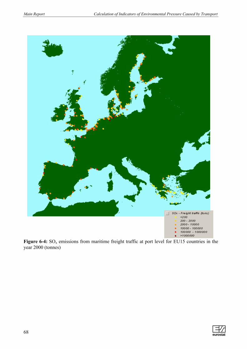
Main Report Calculation of Indicators of Environmental Pressure Caused by Transport
68
Figure 6-4: SOx emissions from maritime freight traffic at port level for EU15 countries in theyear 2000 (tonnes)
eurostat

Calculation of Indicators of Environmental Pressure Caused by Transport Main Report
69
Figure 6-5: SOx emissions from dry bulk carrier traffic for the Baltic area in the year 2000(tonnes)
6.3 INLAND SHIPPINGIn the case of inland shipping, neither the traffic data nor the necessary geographical data for adetailed representation was available. The traffic data provided by EUROSTAT refers to acountry total of tonne-kilometres per year and the results obtained by the simple TRENDS modelare tonnes of pollutants per country per year. Even if the traffic data were available, however, theGISCO database does not include a map of the navigable waterways of EU15 countries so thepollution could not be attributed to linear sources as in the case of railway.
The aim of the GIS part of TRENDS was to sum the pollution from all modes of transport foreach of the individual NUTS region. In this case, the results obtained for inland shipping percountry would have to be divided by the amount of NUTS1 per country before being attributed.However, lack of consistent data to create a base year scenario has lead to this aim beingunattainable, and the representation for inland shipping was kept at country level.
eurostat

Main Report Calculation of Indicators of Environmental Pressure Caused by Transport
70
The results produced for all EU15 countries for a specific year were connected to the NUTS layerusing the country code. In this way all areas within the same country were attributed with thesame value irrespective of their containing navigable waterways.
There was no reason to retain the NUTS segmentation in this situation so shape-merge was usedto produce figure 6-6 which displays the SOx emission from inland shipping in EU15 countriesfor the years 1970, 2000 and 2010 (projection) respectively.
Except for the change in Germany (year 2000) and Sweden (year 2010), no further differencesare observed in the maps, under the present scale scheme, for the years 1970 to 2020.
eurostat

Calculation of Indicators of Environmental Pressure Caused by Transport Main Report
71
Year 1970
Year 2000
Year 2010
Figure 6-6: SOx emissions from inland shipping traffic in the EU15 countries (tonnes)
eurostat

Main Report Calculation of Indicators of Environmental Pressure Caused by Transport
72
6.4 RAILWAYSThe spatial disaggregation of railway emissions was based on the results of the detailed database.
6.4.1 ATTRIBUTING INTRAPLAN-NODES TO GISCO RAILWAY SEGMENTS
The Intraplan [5] traffic database was prepared with the aim to be geographically represented, soa base map was also prepared by Intraplan during the study in the form of a node database.
The node database contains all the important junctions in the rail network, consisting of about1 600 nodes. Each node was defined with a unique number established by the consultants, aname and a set of co-ordinates in the Lambert-Azimuth projection. The co-ordinates weredefined based on the GISCO map for railways and therefore no inconsistency was expected inprojecting data from the two databases together. The problem, however, was that Intraplan used adifferent segmentation and encoding to the one encountered in GISCO without providing acomplete set of co-ordinates for the “nodes” used for the database in their report.
Thus, though the co-ordinates and representation fit, in none of the segmentations present inGISCO are the nodes the same as the ones in Intraplan. What is more, the encoding is completelydifferent so that there can be no manipulation into connecting the two codes. Furthermore,neither INTRAPLAN nor Eurostat were able to provide a link-table when requested, claimingthat the relevant data were no longer present in either their archives. Obviously, an alternativemethod of connecting the databases was required.
After discussions with the GIS team of the Commission, colleagues in Eurostat have attempted tosolve the problem by matching the country code and the two station names (origin, destination)in the emission result tables. In Arc View the two tables were matched on the concatenated“names” with a 95% hit rate. The rest 5% of the entries, still a fair amount, had to be treatedmanually.
These data-points were treated manually due to the name of the station containing characters thatwere not recognised by the database. An effort was made to replace these with English charactersspecific to country groups before matching, but was not successful in all cases, especially sinceerrors existed already.
For example, many problems were created with the Danish links since the special characters æ,ø, å were not taken into account in the substitutions done by Eurostat. Most of these links had tobe treated manually.
Once the connecting table was established, the emission results for each particular link betweentwo nodes could be displayed. The following sets of results were spatially attributed for each ofthe pollutants examined:
− Figure 6-7 : Total emissions from rail traffic activity
− Figure 6-8 : Emission from passenger rail traffic activity – both electric and diesel
− Figure 6-9 : Emission from freight rail traffic activity – both electric and diesel
− Figure 6-10 : Emission from diesel train traffic activity – both passenger and freight
− Figure 6-11 : Emission from electric train traffic activity – both passenger and freight
The possibility for more detailed representation exists, for example by splitting passenger trafficto diesel and electric and even further to locomotives, railcars and high-speed trains for eachengine type.
eurostat

Calculation of Indicators of Environmental Pressure Caused by Transport Main Report
73
Figure 6-7: CO2 emissions from train traffic – both passenger and freight – in EU15 countriesfor the year 1995 (1 000 tonnes)
The above procedure, however, was not successful in connecting the entire Intraplan databaseand the calculated emission results to the GISCO network. In fact, a comparative examination ofthe country totals before and after the connection shows that in most cases a considerable amountof data is lost in the process. The respective fraction based on the results of energy consumptionfor each country is shown in Table 6-1.
Three main reasons are identified for the discrepancies in the data:
1. Despite the effort made, the connecting table may not be complete
2. Intraplan have recorded traffic on ferry links that do not “belong” to a specific country and onlinks between countries that are attributed to a non-EU15 country when summing
3. Intraplan have recorded traffic data for lesser railway links that do not belong to the mainarteries portrayed in the TEN corridors. Traffic on these links is discarded during theconnection process as no station match exists on the main artery layer.
eurostat

Main Report Calculation of Indicators of Environmental Pressure Caused by Transport
74
Figure 6-8: CO2 emission from passenger train traffic in EU15 countries for the year 1995(1 000 tonnes)
Figure 6-9: CO2 emissions from freight train traffic in EU15 countries for the year 1995 (1 000
tonnes)
eurostat

Calculation of Indicators of Environmental Pressure Caused by Transport Main Report
75
Figure 6-10: CO2 emissions attributed to diesel train traffic in EU15 countries for the year 1995(1 000 tonnes)
Figure 6-11: CO2 emissions attributed to electric train traffic in EU15 countries for the year
1995 (1 000 tonnes)
eurostat

Main Report Calculation of Indicators of Environmental Pressure Caused by Transport
76
Table 6-1: Fraction of the actual energy consumption that can be displayed
A more detailed network exists in the GISCO database as well, however, a connection betweenthe two was not possible as, contrary to the attributes of the major arteries, no station names wereincluded in this layer. An attempt was made to spatially join the layers, but the result was notsatisfactory.
In addition to the loss of data discussed above, limitations on the quality of data provided byIntraplan do not allow any conclusions to be drawn on the basis of the presented railway results.For example, the data for freight traffic in Germany, Great Britain, the Netherlands, Sweden andFinland were based on assumptions since no data was supplied by the countries in question.
Whatever the quality of traffic data, however, it is important to observe that the emissionrepresentation follows, by large, the traffic representation in the Intraplan maps. In other words,the procedure of putting the emissions on the map is accurate enough, if provided with reliabledata.
Still some observations can be made. Links with heavy traffic can be acknowledged though thedifference in train energy consumption between the countries and the different types of trainsprevent the relationship from being linear. However, the emission of CO2 is directly related toenergy consumption, while other pollutants are more dependent on other factors, the type ofpower plant for example in the case of SOx.
6.4.2 ATTRIBUTING RAILWAY SEGMENTS TO NUTS REGIONS
As previously mentioned the goal was to attribute emissions from rail traffic to NUTSadministrative regions in order for them to be added up with emission from other transportmodes. In this way, an emission profile was created for each of the administrative regions.
As in the case of attributing the emissions to the railway network the problem was the lack of aconnecting table stating which administrative region the rail traffic link belonged to. Such a tablewas created by spatially joining the NUTS (polygon) and the railway links (arc) layers inArcView with the layer containing railway stations (point) thus creating a link between the two.This action was necessary since a direct spatial join between the two layers did not have asatisfactory effect. The resulting data table had to be further processed for double entries beforeemission values could be attributed.
However, another issue had to be dealt with, as NUTS regions contained more than one railwaylink, or links extended over more than one NUTS region so that the emission values had to besummed or split accordingly. To make sure that emission values were not taken into accountmore than once, the original values were divided by the number of times the respective railwaylink appeared in the connecting table before being attributed to NUTS regions. Consequently,emission values were summed per NUTS region to produce the final data table that would beprojected.
Country Fraction Country Fraction Country FractionAT 0,66 FI 0,91 LU 1,04BE 0,84 FR 0,77 NL 0,82DE 0,78 GR 0,83 PT 0,61DK 0,63 IE 0,71 SE 0,94ES 0,56 IT 0,67 GB 0,80
eurostat

Calculation of Indicators of Environmental Pressure Caused by Transport Main Report
77
This method of transferring emissions from network to NUTS level was very effective as can beseen from Table 6-2 that displays the difference in the country totals calculated on a NUTS andnetwork level. With the exception of Luxembourg the error is not significant given all the otherassumptions involved.
Table 6-2: Ratio between the NUTS and network country totals based on energy consumptionvalues.
Figures 6-12 and 6-13 show the energy consumption and SOx emission over the EU15 NUTSregions respectively. The effect of the fuel and type of power plant used is evident, especially inthe case of countries such as France where a high energy consumption is not translated into highSOx air pollutant emission due to electric trains powered by nuclear stations.
Country Fraction Country Fraction Country FractionAT 1,06 FI 1,02 LU 0,70BE 1,00 FR 0,99 NL 1,03DE 0,99 GR 1,00 PT 1,05DK 1,00 IE 1,00 SE 1,00ES 0,98 IT 1,01 GB 1,00
eurostat

Main Report Calculation of Indicators of Environmental Pressure Caused by Transport
78
Figure 6-12: Total energy consumption by rail traffic activities in the EU15 countries attributedto the NUTS administrative regions – Year 1995
eurostat
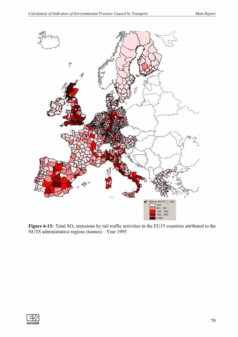
Calculation of Indicators of Environmental Pressure Caused by Transport Main Report
79
Figure 6-13: Total SOx emissions by rail traffic activities in the EU15 countries attributed to theNUTS administrative regions (tonnes) – Year 1995
eurostat

Main Report Calculation of Indicators of Environmental Pressure Caused by Transport
80
7 TEMPORAL DISAGGREGATION – ROAD TRANSPORT
7.1 DATA AVAILABILITYOne of the aims of this project was to attempt to quantify temporal variations of vehicle emissionsand to distribute the annual emissions (for 1995) of EU15 countries on a seasonal basis. Due tolack of relevant data, this procedure was conducted only for the road transport mode.
In order to enable the disaggregation of emissions (via activity data disaggregation) to seasonallevels, appropriate patterns were collected, analysed and consolidated. As Eurostat data onseasonal variation of transport activities were scarce, other sources of information wereinvestigated. Finally, the temporal distribution of vehicle emissions was conducted usingstatistical data from a project conducted by the University of Graz [4]. This project contains astudy of the traffic load for different vehicle and road types, depending on various time-relatedparameters. More specifically, the traffic load of both urban roads and highways was recorded ona weekly and daily basis. The study also discriminated between passenger cars and heavy-dutyvehicles. Weekly variations of the traffic load provided by this source were used in order toproduce the required seasonal variations of vehicle emissions.
7.2 METHODOLOGYFigure 7-1 gives an example of the recorded variations of the weekly traffic load over an entireyear. Each weekly variation in Figure 7-1 is represented as a deviation from an average trafficload.
Seasonal values were determined by calculating the average value of the deviation over the 13weeks that correspond to each season. Since traffic load data were available for several urbanroads the final seasonal variation factors were obtained by averaging over the values of thevarious roads. Finally, CO2, NOx and PM emissions produced by TRENDS for all EU15countries were multiplied with the seasonal deviation factors in order to obtain the requireddistribution of vehicle emissions.
eurostat

Calculation of Indicators of Environmental Pressure Caused by Transport Main Report
81
Figure 7-1: Example of the weekly traffic load variations measured at an urban road over anentire year.
7.3 RESULTSFigures 7-2 to 7-4 show the seasonal variation of CO2, NOx and PM emissions respectively, forGermany and Greece. Figures 7-5 to 7-7 and Figures 7-8 to 7-10 show the seasonal distributionof the aforementioned pollutants in the case of heavy-duty vehicles and highways respectively.The seasonal distribution of CO2, NOx and PM emissions for all EU15 countries is presented inTables A-1 to A-4 of Appendix A.
The large deviation between the annual emissions in Germany and Greece that can be observedfrom these figures is due to the difference in vehicle populations between the two countries.
From Figures 7-2 to 7-10 it is also apparent that the levels of vehicle emissions are higher duringthe summer, which is to be expected since there is an increase in transportation during thesummer holidays.
From Figure 7-4 it can be observed that the yearly PM emissions in Germany are considerablyhigher than the respective emissions in Greece. The difference in annual emissions between thetwo countries is more pronounced in the case of PM emissions than in the case of otheremissions. This is due to the fact that the number of diesel PCs in Greece is significantly lowerthan that of Germany, because according to the Greek legislation, diesel PCs are only allowed foruse as taxis. Since PM emissions are produced almost entirely by diesel vehicles, PM emissionsfor PCs in Greece are extremely low.
eurostat

Main Report Calculation of Indicators of Environmental Pressure Caused by Transport
82
Figure 7-2: Seasonal distribution of annual (1995) CO2 emissions for PCs in Germany andGreece
Figure 7-3: Seasonal distribution of annual (1995) NOx emissions for PCs in Germany andGreece
Comparison of seasonal CO2 emissions for PCs between Germany and Greece
0
5.000
10.000
15.000
20.000
25.000
30.000
35.000
Spring Summer Autumn Winter
CO
2 [1
000
t]
GermanyGreece
Comparison of seasonal NOx emissions for PCs between Germany and Greece
0
20.000
40.000
60.000
80.000
100.000
120.000
140.000
160.000
180.000
200.000
Spring Summer Autumn Winter
NO
x [t] Germany
Greece
eurostat
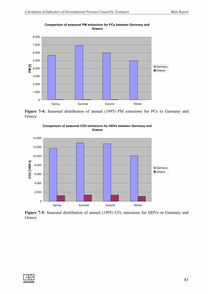
Calculation of Indicators of Environmental Pressure Caused by Transport Main Report
83
Figure 7-4: Seasonal distribution of annual (1995) PM emissions for PCs in Germany andGreece
Figure 7-5: Seasonal distribution of annual (1995) CO2 emissions for HDVs in Germany andGreece
Comparison of seasonal PM emissions for PCs between Germany and Greece
0
1.000
2.000
3.000
4.000
5.000
6.000
7.000
8.000
Spring Summer Autumn Winter
PM [t
]
GermanyGreece
Comparison of seasonal CO2 emissions for HDVs between Germany and Greece
0
2.000
4.000
6.000
8.000
10.000
12.000
14.000
Spring Summer Autumn Winter
CO
2 [1
000
t]
GermanyGreece
eurostat

Main Report Calculation of Indicators of Environmental Pressure Caused by Transport
84
Figure 7-6: Seasonal distribution of annual (1995) NOx emissions for HDVs in Germany andGreece
Figure 7-7: Seasonal distribution of annual (1995) PM emissions for HDVs in Germany andGreece
Comparison of seasonal NOx emissions for HDVs between Germany and Greece
0
20.000
40.000
60.000
80.000
100.000
120.000
140.000
Spring Summer Autumn Winter
NO
x [t] Germany
Greece
Comparison of seasonal PM emissions for HDVs between Germany and Greece
0
2.000
4.000
6.000
8.000
10.000
12.000
14.000
Spring Summer Autumn Winter
PM [t
]
GermanyGreece
eurostat

Calculation of Indicators of Environmental Pressure Caused by Transport Main Report
85
Figure 7-8: Seasonal distribution of annual (1995) CO2 emissions for highways in Germany andGreece
Figure 7-9: Seasonal distribution of annual (1995) NOx emissions for highways in Germany andGreece
Comparison of seasonal CO2 emissions for highways between Germany and Greece
0
2.000
4.000
6.000
8.000
10.000
12.000
14.000
16.000
Spring Summer Autumn Winter
CO
2 [1
000
t]
GermanyGreece
Comparison of seasonal NOx emissions for highways between Germany and Greece
0
20.000
40.000
60.000
80.000
100.000
120.000
140.000
Spring Summer Autumn Winter
NO
x [t] Germany
Greece
eurostat

Main Report Calculation of Indicators of Environmental Pressure Caused by Transport
86
Figure 7-10: Seasonal distribution of annual (1995) PM emissions for highways in Germany andGreece
Comparison of seasonal PM emissions for highways between Germany and Greece
0
1.000
2.000
3.000
4.000
5.000
6.000
Spring Summer Autumn Winter
PM [t
]
GermanyGreece
eurostat

Calculation of Indicators of Environmental Pressure Caused by Transport Main Report
87
8 PROBLEMS AND SHORTCOMINGS OF THE PRESENT SYSTEM
8.1 ROAD TRANSPORT MODULEQuantity and quality of data
• Data on load factors and occupancy rates are scarce (not available for all EU countries, norfor all years; corresponding data for urban-rural-highway driving conditions are notavailable), thus not allowing for an accurate estimation of specific emissions (indicators). Theaccuracy of the data on LF and OR obtained so far is ambiguous
• The input data for some countries are poor. Consistency checks on the basis of fuelconsumption data are required (following the example of COPERT, these checks could beintroduced in the module instead of being performed externally).
• Statistical data for the temporal disaggregation (seasonal, monthly, diurnal profiles) ofemissions are not available
• Waste calculation: Validation of emission factors is still required
Technical issuesThe system is unable to handle the introduction of new technologies (e.g. post Euro V vehicles).In this sense, scenarios based on alternative technologies cannot be simulated.
In addition, scenarios including changes in the vehicle fleet composition and the life timefunction parameters (e.g. scrappage schemes) can only be performed by expert users (either bychanging the LTF parameters, or by introducing vehicle fleet data for specific years)
Geographical coverageThe software was designed to calculate road transport parameters for the EU15 Member Statesonly and does not allow the introduction of new countries. Thus, if new countries are to beincluded (e.g. Candidate countries, cf. ETC/ACC requirements) the structure of the systemrequires significant modifications
Moreover, the module does not calculate EU totals. This function is performed externally,through an Excel-based module
Lack of flexibilityAll output values should be easy to handle. Export facilities for obtaining the data in predefinedformats are required. If TRENDS is to be used as a source of data for ETC/ACC or otheractivities, then the user requirements must be specific from the very beginning. The options ofeither producing one (or more) exports per country and a “total” export for all countries must beavailable.
The software operates only under a specific version of Microsoft Access (Access 97). Moreover,it exhibits occasional failures and errors during the data calculation
The system was designed for expert users only. Changes in the input data are rather complex(although there should be options to allow users to enter other than the “default” values at everystep of the calculation). Minor alterations and additions in the software require radical changes inthe input tables
eurostat

Main Report Calculation of Indicators of Environmental Pressure Caused by Transport
88
8.2 RAILWAY, MARITIME AND INLAND SHIPPING MODULESQuantity of input data
• The traffic data available for all modes is limited to a small number of years
• Projections for future years are not available
Quality of input data
• The data available is more of statistical interest than suitable for calculations
• Discrepancies in the data are very common
Lack of evaluation
• There is very limited information as to the accuracy of the model
Requires expert user
• The management and use of the database requires an experienced user that is familiar withthe data and system limitations
Access has proved unstable and “difficult” as a platform
• Lack of flexibility means that minor changes may require major restructuring in the database
• Software may not run smoothly in all systems
8.3 AIR MODULEQuantity of input data
• Detailed traffic data is only available for IFR flights in Europe from 1996 onward
• Projections for future years are not available in the same degree of detail
Quality of input data
• Data available consist of flight plan information not actual flights, which can lead todiscrepancies mainly due to congestion, changes in schedule etc.
• No information is available on number of passengers or cargo carried per flight
Lack of knowledge on several components
• No information is available on PM10 and PM2.5 emissions
• Only draft estimates are available on components like CH4, NH3, N2O
• Only estimates are available for additional ground emissions like engine start and auxiliarypower unit, which are not covered by the standard LTO cycle
eurostat

Calculation of Indicators of Environmental Pressure Caused by Transport Main Report
89
9 FUTURE DEVELOPMENTSFurther development is aimed at:
Focusing the role of TRENDS on the production of TERM indicators
• The outline of the TRENDS program was designed prior to TERM, with the intention ofproviding indicators related mainly to air pollution and energy consumption. TRENDS isnow regarded as the main production tool for TERM indicators. How could TRENDS bebetter adapted to the needs of TERM? In particular what other TERM indicators could beproduced within TRENDS, and what data-sets would be needed for their calculation?
Improving the efficiency of the software
• The current system is based on MS Access. It has proved difficult to revise coding. Otheralternatives should be investigated and a more appropriate software package should beconsidered in the future.
Expanding or reducing coverage
• TERM is currently being extended to cover non-EU countries. The development of TRENDSshould be considered in order to include the countries of the European Economic Area(Iceland, Liechtenstein, Norway), Switzerland, and the Candidate countries (Bulgaria,Cyprus, Czech Republic, Estonia, Hungary, Lithuania, Latvia, Malta, Poland, Romania,Slovakia, Slovenia and Turkey). A critical factor here is the existence of compatible data.
• TRENDS is linked to a GIS system which provides a regional disaggregation of emissions, aswell as a split between urban, rural and highway areas for one base year. Is it appropriate anduseful for TRENDS to attempt such regional disaggregation? Or should this link bedeveloped?
• The aviation module covers only the years 1996-2001. The calculating tool needs to beexpanded to produce estimates for all years in the time frame 1970-2020. In order to evaluateair emissions for the missing years, additional data from Eurostat or other sources arerequired.
• The TRENDS program currently covers waste from road transport. The development ofTRENDS to cover waste from other modes should be considered.
• Would it be feasible to introduce life-cycle analysis (e.g. as within the STEEDS and ASTRAprogrammes [11]) and calculations of external costs (e.g. as developed within ExternE [12])and by INFRAS [13] based on coefficients derived from other programmes, particularly atEU level?
Data issues: better fitting statistics to methods
• Has the optimum use been made of existing data? Are there other sources which were notexploited? Should Eurostat establish a new data collection?
• How can data be more efficiently pre-processed, either externally or within TRENDS?
• What should be endogenous to TRENDS, and what should be exogenous? What sourcesshould be used for exogenous variables? Possible links to other EU projects should beexplored, especially as regards baseline forecasts of transport activity (cf. Scenes [14]).
eurostat

Main Report Calculation of Indicators of Environmental Pressure Caused by Transport
90
• The modelling of road vehicle turnover uses an engineering approach as used in emissionmodels. It has not been adapted for estimating waste, and does not consider scrappageschemes or imports and exports of used vehicles. It is therefore inadequate for estimatingend-of-life vehicles and waste from this stream. What are the alternatives to the currentmethod?
TAB: Revision of basecase scenario - production of additional scenarios
• The assumptions made for the basecase scenario should be discussed and modificationsshould be made, if required.
• Sensitivity runs are required in order to assess the effect of various input parameters on thetraffic activity and emission results produced.
• Apart from the basecase scenario, additional scenarios should be created, in order to take intoaccount various effects, such as the increase of diesel share in recent years, (see section 4.1)which were not considered in the reference scenario.
eurostat

Calculation of Indicators of Environmental Pressure Caused by Transport Main Report
91
REFERENCES
1) L. Ntziachristos and Z. Samaras, COPERT III: Computer programme to calculate emissionsfrom road transport, Methodology and emission factors (Version 2.1), Technical report No49 (2000)
2) LAT, TUV, KTI, TRAP: Study on Transport-Related Parameters of the European RoadVehicle Stock, 1999
3) N. Kyriakis, Z. Samaras and A. Andrias, MEET: Methodologies for Estimating Air PollutantEmissions from Transport - Road Traffic Composition, Task 2.2 - Deliverable 16, LATReport No 9823, 1998
4) Technical University of Graz, KFZ-Emissionskataster Steiermark, Final report January 1992,Report No 7/92 – Stu 1992 02 18
5) Intraplan, Tetraplan, Transport Flows on the European Railway Network, INRETS (1997)
6) Lloyds Register of Shipping (1994), Register of Ships, 1994-1995, London
7) Corbett JJ, P Fischbeck (1997), Emissions from ships, Science, Vol 278, pp 823-824
8) Sorenson S.C., T. Kalivoda, M. Kudrna and P. Fitzgerald Future non-road emission factorsDTU report, (1998) DEL MEET 25
9) UBA Berlin, Umweltbundesamt, Jahresbericht 1995, Berlin
10) European Commission, Standard and Poor’s DRI and K.U. Leuven, Auto-Oil II Cost-Effectiveness Study, Draft final report, 1999
11) http://www.cordis.lu/transport/src/astra.htm.
12) http://externe.jrc.es.
13) http://www.infras.ch.
14) http://www.iww.uni-karlsruhe.de/SCENES
eurostat

APPENDIX A: SEASONAL DISTRIBUTION OF CO2, NOX AND PM EMISSIONSTable A-1: CO2, NOx and PM vehicle emissions for spring
Table A-2: CO2, NOx and PM vehicle emissions for summer
eurostat

Table A-3: CO2, NOx and PM vehicle emissions for autumn
Table A-4: CO2, NOx and PM vehicle emissions for winter
eurostat


