Calculation of the Optimal Filtering Coefﬁcients and...

UNIVERSIDAD AUTONOMA DE MADRID (UAM)DEPARTAMENTO DEFISICA TEORICA

Calculation of the Optimal Filtering Coefficientsand check of the signal reconstruction for the

ATLAS Electromagnetic Calorimeter

Ph.D. DEA: Carolina Gabaldon RuizSupervisor: Dr. Jose Del Peso Malagon

2

Agradecimientos

Este trabajo no se habrıa podido realizar sin la colaboracion de muchas personas queme han brindado su ayuda, sus conocimientos y su apoyo. Quiero agradecerles a todosellos cuanto han hecho por mı, para que este trabajo salieraadelante de la mejor maneraposible.

En primer lugar, quiero expresar mi agradecimiento a mi tutor Jose del Peso. Gra-cias Jose porque sin ti no hubiera sobrevivido en el CERN, hassabido dirigir mi trabajo enestos dos anos y enfocarlo con exito. He aprendido contigoque si quieres algo lo puedesconseguir, solo tienes que esforzarte.

De igual manera, mi mas sincero agradecimiento al directordel grupo FernardoBarreiro a quien debo el realizar el doctorado en el grupo de Altas Energıas de la Univer-sidad Autonoma de Madrid. Gracias por la confianza que has depositado en mi y por tuinteres por mi trabajo.

A Eduardo le agradezco profundamente su apoyo en los momentos difıciles. Gra-cias por estar siempre dispuesto a ayudarme en el trabajo y enla vida. Ha sido un placercompartir el tiempo de la universidad y de estos dos anos de doctorado contigo.

A toda la gente del grupo de Altas Energıas, gracias por haberme aceptado comoparte del grupo. En particular, muchas gracias a Luis Labarga por haber podido contarcon sus conocimientos de fısica y por las charlas mantenidas. A todos los del laboratorio,por su paciencia conmigo en el campo de la informatica y comoamigos.

Un mencion especial a Pascal Pralavorio que me ha ayudado enel CERN y mehan ensenado realmente ha apreciar la fısica y ha creer quepodriamos realizar un buentrabajo. Gracias por formar un equipo conmigo.

Agradecer hoy y siempre a mi familia, mi madre y mi hermano, los tres formamosun equipo. Mama gracias porque sin ti no habrıa podido empezar, ni terminar la carrera yporque siempre has estado conmigo en los malos y buenos momentos. Y a Nicola porquetiene la facultad de convertir todas las cosas malas en buenas y porque siempre esta a milado.

Contents

1 Introduction 5

2 LHC machine and ATLAS detector 7

2.1 LHC . . . . . . . . . . . . . . . . . . . . . . . . . . . . . . . . . . . . . 7

2.2 The ATLAS experiment . . . . . . . . . . . . . . . . . . . . . . . . . . . 9

2.2.1 Inner Detector . . . . . . . . . . . . . . . . . . . . . . . . . . . 10

2.2.2 The calorimeters . . . . . . . . . . . . . . . . . . . . . . . . . . 11

2.2.3 The muon spectrometer . . . . . . . . . . . . . . . . . . . . . . . 14

3 ATLAS Electromagnetic calorimeter 17

3.1 Performance requirements . . . . . . . . . . . . . . . . . . . . . . . . .17

3.2 Generalities of the EM calorimeter . . . . . . . . . . . . . . . . . .. . . 18

3.3 End-cap specifities . . . . . . . . . . . . . . . . . . . . . . . . . . . . . 20

3.4 Barrel specifities . . . . . . . . . . . . . . . . . . . . . . . . . . . . . . 23

3.5 Segmentation . . . . . . . . . . . . . . . . . . . . . . . . . . . . . . . . 24

3.6 High Voltage . . . . . . . . . . . . . . . . . . . . . . . . . . . . . . . . 25

3.7 Electronics . . . . . . . . . . . . . . . . . . . . . . . . . . . . . . . . . 28

3.8 Some differences between EMEC and EMB . . . . . . . . . . . . . . . .30

4 Signal Reconstruction Algorithms 33

4.1 Optimal filtering method . . . . . . . . . . . . . . . . . . . . . . . . . . 33

4.1.1 Prediction of physics pulse . . . . . . . . . . . . . . . . . . . . . 35

4.2 Computation ofgphys . . . . . . . . . . . . . . . . . . . . . . . . . . . . 39

1

2 CONTENTS

4.3 Parameter extraction algorithm (RTM) . . . . . . . . . . . . . . .. . . . 40

5 Signal reconstruction in the end-caps 45

5.1 Inputs for the end-caps . . . . . . . . . . . . . . . . . . . . . . . . . . . 45

5.1.1 Cell response to a calibration signal . . . . . . . . . . . . . .. . 45

5.1.2 Calibration board parameters . . . . . . . . . . . . . . . . . . . .46

5.1.3 Ion drift time in liquid argon gap . . . . . . . . . . . . . . . . . .47

5.1.4 Electronic chain characteristics . . . . . . . . . . . . . . . .. . . 48

5.1.5 Summary of the inputs . . . . . . . . . . . . . . . . . . . . . . . 52

5.2 Outputs of the method . . . . . . . . . . . . . . . . . . . . . . . . . . . 53

5.2.1 Computation of the pulse shapes and optimal filtering coefficients for physics 53

5.2.2 Estimation of the calibration bias . . . . . . . . . . . . . . . .. 54

5.2.3 Noise reduction with optimal filtering technique . . . .. . . . . . 55

6 Cosmic runs 59

6.1 Origin of cosmic muons . . . . . . . . . . . . . . . . . . . . . . . . . . . 59

6.2 Energy loss due to ionization . . . . . . . . . . . . . . . . . . . . . . .59

6.3 Energy loss by radiation: Bremsstrahlung . . . . . . . . . . . .. . . . . 63

6.4 Calorimeters setup for cosmic runs . . . . . . . . . . . . . . . . . .. . . 64

7 Checking signal reconstruction in|η| < 3.2 with cosmic data 69

7.1 Selection of high energy deposits . . . . . . . . . . . . . . . . . . .. . . 69

7.1.1 Conditions of data taking . . . . . . . . . . . . . . . . . . . . . . 70

7.1.2 Selection criteria . . . . . . . . . . . . . . . . . . . . . . . . . . 71

7.1.3 Map of selected cells . . . . . . . . . . . . . . . . . . . . . . . . 72

7.2 Comparison of predicted physics pulse shapes with data .. . . . . . . . . 73

7.2.1 Method to superimpose predictions and data . . . . . . . . .. . . 73

7.2.2 Quality of the predicted pulse shapes . . . . . . . . . . . . . .. 77

7.2.3 Main systematic uncertainty in the end-cap signal reconstruction . 80

7.2.4 Influence of the ion drift time on the pulse shape description . . . 81

CONTENTS 3

8 Conclusions 85

4 CONTENTS

Chapter 1

Introduction

In the 20th century, particle physics experiments have proven crucial for our understand-ing of nature. Particle accelerators like the Large Hadron Collider (LHC) boost subatomicparticles to nearly the speed of light, before letting them collide. The extreme energy den-sities in these collisions are similar to those that existedjust after the Big Bang, when theuniverse was created. Hence, the LHC results may give some lights on the understandingof the early stages of the Universe.

The particles that are created in the collisions are detected by a particle detector.These detectors are extraordinarily complex, requiring years of research and development.The work of the present ”tesina” is related to one of the general purpose LHC experiments,ATLAS, and in particular, it is about the calibration of the liquid Argon ElectromagneticCalorimeter using cosmic muon data.

The EM calorimeter is installed in the ATLAS cavern since theend of 2006. Beforethe LHC start, the main challenge is to operate coherently its∼ 170000 channels, whichimplies the commission of the associated electronics, the determination of the calibrationconstants, the reconstruction of the signal amplitude froma digital filtering technique(Optimal Filtering Method) and the development of automation algorithms among othertasks.

Many of the physics process to be measured in ATLAS from proton-proton collisionwill have electrons or photons in the final state.Higgs→ γγ, Higgs→ e+e−e+e− orZ′ → e+e− are some examples among them. The measurement of the energy and directionof these final state particles put strict requirements in theconstruction and calibration ofthe Electromagnetic Calorimeter. In particular a very goodsignal reconstruction, at thelevel of 1%, is demanded.

The signal reconstruction method, adopted for the ATLAS Electromagnetic Calorime-ter, is based on an accurate knowledge of the calorimeter cells properties and the elec-

5

6 CHAPTER 1. INTRODUCTION

tronic chain characteristics [11]. It has been checked and tuned in the past using electronsbeams of known energy for the Electromagnetic Barrel (EMB) Calorimeter [12, 14]. Inthis ”tesina” the signal reconstruction method is applied for the first time to the End-CapElectromagnetic Calorimeter (EMEC) and tested using cosmic muon data.

At present, cosmic muons are the only possible real data before the starting of theLHC. They have been used recently for doing some uniformity studies and timing per-formance in the EMB Calorimeter [15]. Other sub-detectors operational in the ATLASpit can be used as trigger for these muons. In particular, in the present work the triggerwas defined by the Hadronic Tile Calorimeter (TileCal), which surrounds the EMB andEMEC calorimeters. In contrast to the EMB calorimeter, the muons entering the EMECare not projective to the nominal ATLAS center (or nominal interaction point). As a con-sequence only muon events with high energy deposits, for instance those which radiate abremsstrahlung photon in their way through the calorimeter, produce a detectable signalin the EMEC. The photon generates an electromagnetic cascade at a certain location in-side the calorimeter with enough energy deposition for the purpose of the present studies.The number of such muons is however a small fraction of the total triggered by the Tile-Cal. These events are selected and analysed in both parts EMBand EMEC for the firsttime.

The EMEC, much less tested so far, will have the main focus in this analysis. How-ever, a detailed comparison between EMEC and EMB is also provided, which is particu-larly important as:(i) the same reconstruction scheme will be applied for the barrel andthe end-cap parts;(ii) the geometry of the latter is more complicated than the former withthe consequence that most electrical parameters vary by a factor 2−3 over the end-capη-coverage, whereas they are almost constant in the barrel part. This requires intensivecross-checks to avoid any systematic bias.

Although the emphasis in this document will be put in the analysis of the cosmicmuon data to check the signal reconstruction method in the EMEC, the work has alsoinvolved the production of all calibration constants for the EMEC, for its more than 60,000cells or channels. In particular all the predicted physics pulse shape and Optimal FilteringCoefficients have been computed and recorded in the Conditional Data Base for use inany physics analysis by any member of ATLAS.

The outline of this ”tesina” is as follows. In Chapter 2 an overview of the ATLASexperiment is given. Chapter 3 recalls the main characteristics and specificities of the EMcalorimeter. Chapter 4 describes the algorithms used to thereconstruction of the signal inthe EM calorimeter. Chapter 5 details the inputs needed for the signal reconstruction andestimates the calibration bias and the noise reduction linked to the method. In Chapter 6some generalities about cosmic muons and the ATLAS setup forthe muon tests are cov-ered. Chapter 7 gives the results of the quality checks performed with the cosmic muondata. Finally, Chapter 8 is dedicated to conclusions.

Chapter 2

LHC machine and ATLAS detector

2.1 LHC

The Large Hadron Collider(LHC) [1] will become CERN’s main accelerator complex.It is currently under construction in the same tunnel that was used for LEP accelerator,which was decommissioned in 2000. The LHC will accelerate two counter-rotating pro-tons beams to an energy of 7 TeV, which will collide head-on atfour points along the ring.The resulting interactions have an unprecedented center ofmass energy of 14 TeV, whichwill allow physicist to study new field of physics. The startup is scheduled for summer2008.

The acceleration of the protons starts at a dedicated linearaccelerator (linac), whichaccelerates bunches of 1011 protons to an energy of 50 Mev. These bunches are thentransferred to the PS Booster (PSB), where the energy is increased to 1.4 GeV. The energyis further increased to 26 GeV by the Proton Synchrotron (PS). The protons are theninjected into the Super Proton Synchrotron (SPS) where theyare accelerated to 450 GeV.Finally, the SPS injects the protons clockwise and counter-clockwise into the LHC ring,where they are accelerated to their final energy of 7 TeV. Morethan 1200 dipole magnetsare installed along the LHC ring to keep the protons on track in the ring. The dipolesprovide a magnetic field of up to 9 Tesla. The main parameters of the LHC acceleratorare given in table 2.1.

Like its center of mass energy, the luminosity of the LHC is also unprecedented fora proton collider. The luminosity is defined as the number of protons that pass by, per unitarea, per unit time. The higher the luminosity, the more proton-proton interactions persecond will occur. At the LHC design luminosity of 1034 cm−2s−1, on average about 27interaction will occur per bunch crossing, with a bunch spacing of 25 ns. Thus the numberof proton-proton interactions per second will be around 109. Such high luminosity is

7

8 CHAPTER 2. LHC MACHINE AND ATLAS DETECTOR

needed because many interesting physics processes at the LHC energy have very smallcross section, 1 pb or less (1 pb=10−36 cm2).

Parameter Value Unit

Circumference 26659 mBeam energy 7 TeV

Injection energy 0.45 TeVDipole field at 450 GeV 0.535 T

Dipole field at 7 TeV 8.33 THelium temperature 1.9 K

Coil aperture 56 mmDistance between apertures194 mm

Luminosity 1034 cm−2s−1

Luminosity lifetime 10 hBunch spacing 25 ns

Particles per bunch 1011

Bunches per beam 2808

Table 2.1:Main LHC parameters

Four detectors are under construction at the points where the beams collide: ALICE,ATLAS,CMS and LHCb. ATLAS and CMS are general purpose detectors, i.e. they aredesigned to cover a wide range of physics. Their primary taskwill be to discover theHiggs particle (if it exist), but they will also explore the physics beyond the Standardmodel, like supersymmetry, extra dimension, and even mini black holes. The ATLASexperiment is described in more detail in the next section.

The LHCb experiment is dedicated to the study of CP-violation in the B-system,itis therefore optimized for the detection of B-mesons. LHC uses a low luminosity beamof about 1032 cm−2s−1, by defocusing the proton beams near the interaction point.Thisis needed because the production and decay vertices of the B-mesons are difficult to re-construct if there is more than one interaction per bunch crossing.

The ALICE experiment focus on the study of the quark-gluon plasma, by measur-ing the particles that are produced in heavy ion collisions.The quark-gluon plasma is ahadronic state where quarks and gluons are not in bound statelike protons anymore, butmove freely in the plasma. It is expected that the extreme energy densities in the heavyion collision is sufficient to create this state of matter fora fraction of a second.

2.2. THE ATLAS EXPERIMENT 9

2.2 The ATLAS experiment

The ATLAS detector is currently under assembly at ’point 1’,the interaction point near theCERN Meyrin site. Like most colliding beam experiments it has approximate cylindricalsymmetry. The detector is organized in a central barrel where the detection elementsform cylindrical layers around the beam pipe, and two end-caps organized in cylindricalwheels. Figure 2.1 gives an overall view of the detector.

Figure 2.1:Overview of the ATLAS detector. The various subsystems havebeen indicated

The cylindrical symmetry makes a polar coordinate system useful. The direction ofthe proton beams is the z-axis, being zero the ATLAS center ornominal interaction pointand positivez values corresponds to the side where the End-Cap A is located. The originfor the azimuthal angle (Φ) points to the center of the LHC ring (x-axis), while the originof the polar angleθ is the positivez-axis. Instead of the polar angleθ, the pseudorapidityη = −log(tan(θ/2)) is used. The pseudorapidity is a convenient quantity because theparticle multiplicity is approximately constant as a function of η. The name comes fromthe fact that the pseudorapidity of a particle in the massless limit is equal to the rapidityy = 1

2logE+pzE−pz

.

ATLAS consist of three subsystems. The inner-most system isthe inner detector,which detects the track of changed particles. The energy of the particles and jets are mea-sured by the calorimeters, which are built around the inner detector. And in the outer-most


part, the muon spectrometer to detect the muons, which scapethe calorimeters. ATLAS is45 meters long and 22 meters high, which makes its volume an order of magnitude largerthan previous collider experiments. This is a direct consequence of the 14 TeV centerof mass energy of the LHC beams. The large volume give the trackers a long level arm,which improve the momentum resolution, particularly at high momenta. Thick calorime-ters are required to fully contain the shower in the calorimeter, and reduce the amount ofpunch-through into the muon chambers to a minimum. Fast electronics are required to”keep up” with the bunch crossing rate, which is also higher than in previous experiments.

A large number of particles is expected to be produced in the proton collisions.Many of those particles are grouped into jets. Since jets often have a large boost, theparticles in a jet are nearly collinear. A detector with fine granularity is required to dis-tinguish particles within a jets. Since the particle flux decreases as a1R2 , the requirementof granularity become less important for the detector elements that are further away fromthe interaction point.

The basic design criteria of the ATLAS detector are:

• Very good electromagnetic calorimeter for electron and photon identification andenergy measurement, complemented by full-coverage hadronic calorimetry for ac-curate jet and missing traverse-energy measurements;

• High-precision muon momentum measurements, with the capability of guaranteeaccurate measurements at high luminosity using the external muon spectrometer;

• Efficient tracking at high luminosity for momentum measurement of highpT lep-tons, electron identification,τ-lepton and heavy-flavor identification, and full event-reconstruction capability.

• Large acceptance in pseudo-rapidity with almost full azimuthal angle coverage ev-erywhere.

• Triggering and measurements of particles at low-pT threshold, providing high effi-cient for most physics processes at LHC.

2.2.1 Inner Detector

The Inner Detector(ID) system [2] covers the acceptance range |η| < 2.5, matching thatof the rest of the ATLAS sub-detectors for precision physics. The ID, thanks to the tracksbending provided by the solenoid magnet, is responsible to measure the momentum of thecharged particles coming from the interaction point. Together with the electromagneticcalorimeter, it provides the identification of electrons and photons. Its tracking capabilityallows to reconstruct secondary vertex from the decay ofτ leptons and b-flavored hadrons.


Figure 2.2:Tridimensional cut-away view of the ATLAS inner detector system

The ATLAS ID tracking system (figure 2.2) is composed of threedifferent subde-tectors layers:

• The Pixel Detector (PD)is a finely segmented silicon detector located in the ra-dial range between 4 and 22cm from the beam line. The PD is composed of 3different layers, located at increasing radio and designedto give 3 space points pertrack. The first pixel layer gives a substantial contribution to the secondary vertexmeasurements, and is designed to be replaceable due to the very hostile radiationenvironment.

• The Semiconductor Tracker (SCT)is a silicon detector located in the radial rangebetween 22 and 56cm. It is divided in barrel and end-cap parts. The barrel uses 4layers of silicon micro-strips to provide precision pointsin space.

• Transition Radiation Tracker(TRT) is based on the use of straw tubes that canoperate at very high rate. The straw tubes are filled with a gasmixtureXe/CO2/O2.The straws are interleaved with polypropylene foils for theidentification of elec-trons through the transition radiation effect.

2.2.2 The calorimeters

The calorimetry system in the ATLAS detector identifies and measures the energy ofparticles (both charged and neutral) and jets. It also detects missing transverse energy bysumming all the measured energy deposit:Emiss

T =√

(∑ETcosφ)2+(∑ETsinφ)2, whereET = Ecell cos(θcell).


The calorimeters contain dense materials (absorber), which cause an incoming par-ticle to initiate a shower. Particles that are created in this shower are detected in the activematerial, which is interleaved with the absorbers. The total signal in the active materialis proportional to the energy of the incoming particle. ATLAS uses two types of activematerial: liquid argon (LAr) and scintillating plastic. Charged particles that traverse theliquid argon create charge by ionization, which is collected on readout electrodes. Thescintillating plastic is doped with fluorescent dye molecules, which emit light when theatoms in the plastic are excited by the crossing of a charged particle. This light is detectedand amplified by photomultiplier tubes. For the absorbers several different types of mate-rial are used, depending on factors like space constraints and ease of manufacturing: lead,iron, copper and tungsten. The location of the calorimetersis shown in figure 2.3. Thepseudorapidity coverage by the whole calorimetry system is|η| ≤ 4.9.

Figure 2.3:Right side’s schematic view of the calorimeter systems in ATLAS.

The electromagnetic calorimeter

The electromagnetic calorimeter [3] identifies electrons and photons and measures theirenergy. It consists of a barrel (0< |η| < 1.475) and two end-caps (1.375< |η| < 3.2 ). Ituses liquid argon as the active medium and lead absorber plates as the passive medium.


The lead plates are folded into an accordion shape. This configuration prevents cracksalongφ, which would degrade the energy resolution. The readout electrodes, made ofcopper and kapton, are installed between the lead plates.

The electrodes are separated from the lead by spacer meshes.The remaining spaceis filled with liquid argon. The argon is cooled by a cryostat system; the barrel part sharesthe same cryostat vessel with the solenoid magnet. The barrel and end-cap modules are di-vided into three longitudinal compartments (samplings). The front compartment is finelysegmented in|η|, which makes a goodγ/π0 ande/π separation possible. The middle com-partment is the deepest, hence contains most of the shower energy generated by incidentelectrons or photons. The last compartment is used to complete the energy measurementof showers for higher energies and for estimations of leakage behind the calorimeter. Inthe following chapter is given a detailed description of theLAr Calorimeter.

The hadronic calorimeter

The hadronic calorimeter [4] is built around the electromagnetic calorimeter. It willmeasure the energy and direction of jets of particles, formed by the hadronization ofquarks and gluons, and by hadronically decayingτ−leptons. The barrel part, called thetile calorimeter, consists of a central barrel (0< |η| < 1.0) and two extended barrels(0.8 < |η| < 1.7). The tile calorimeter uses iron plates as the absorber, which also serveas the return yoke for the solenoid magnet. The active mediumis formed by scintillatorplastic tiles, which are read out on both sides by optical fibers. The tiles are placed radi-ally, normal to the beam line, and are staggered in depth. Cells are formed by groupingtiles together. The calorimeter has three compartments or samplings in depth read outindependently. The readout cells are approximately projective to the interaction point,and have a granularity ofδη×δφ = 0.1×0.1 ( 0.2×0.1 in the third sampling). The totalnumber of channels is about 10,000.

The end-cap hadronic calorimeter uses liquid argon technology, because of its higherradiation tolerance. It uses 25 and 50 mm copper plates as theabsorber material, arrangedin a parallel-plate geometry. The 8.5 mm gaps between the copper plates have three par-allel electrodes, thus dividing the gap into four 1.8 mm drift spaces. Smaller drift spacesrequire a lower voltage (typically 2 kV instead of 4 kV) whichreduces the risk of ionbuild-up and discharge currents. Hadronic showers are muchlonger than electromagneticshowers, and also much wider. Therefore the hadronic calorimeter needs to be muchthicker than the electro-magnetic calorimeter. The total thickness of the calorimeters ismore than 10λ, whereλ is the interaction length (the mean free path of a hadron be-tween two interactions). This is sufficient to stop almost all the particles that are createdin the shower, except muon and neutrinos. However, the calorimeters produce a largebackground for the muon detector, that consists mainly of thermalized slow neutrons andlow-energy photons from the hadronic shower. The Hadronic End-Cap calorimeter is


segmented longitudinally in 4 compartments.

The forward calorimeter

The forward calorimeter (FCAL) is a copper-tungsten calorimeter. It covers the region3.1 < |η| < 4.9. It is split longitudinally into an electromagnetic compartment, and twohadronic compartments. The copper and tungsten have a regular grid of holes that holdthe tube- and rod-shaped electrodes. The space between the tubes and rods is filled withliquid argon. The FCAL is integrated in the same cryostat as the electromagnetic andhadronic end-cap calorimeters.

2.2.3 The muon spectrometer

The muon system [5] is by far the largest subdetector in ATLAS. High−pT muons area signature of interesting physics, therefore the muon trigger and reconstruction is veryimportant. The muon system is designed to achieve a momentumresolution of 10% for 1TeV muons. Fig 2.4 gives an overview of the detector layout.

chamberschambers

chambers

chambers

Cathode stripResistive plate

Thin gap

Monitored drift tube

Figure 2.4:Three-dimensional view of the ATLAS muon spectrometer

The magnet system in the muon detector is completely independent from the inner


detector. It consists of eight superconducting coils in thebarrel, and one eight coils eachtoroid per end-cap. The magnet is an air-core magnet system,i.e. the space between thecoils is left open. Filling this space with iron would enhance the field strength and wouldalso make the field more uniform, but it would also induce multiple scattering that woulddegrade the momentum resolution. The air-core system has anaverage field strength of0.5 T. Four types of detection chambers are used in the muon system: Monitored DriftTube (MDT) chambers, Resistive Plate Chambers (RPCs), ThinGap Chambers (TGCs)and Cathode Strip Chambers (CSCs). The MDT chambers provideprecise muon trackingand momentum measurement. The chambers consist of aluminium tubes with a 30 mmdiameter and a central wire.A muon that crosses a tube will produce ionization clusters inthe gas (Ar/CO2), which will drift to the wire. The distance between the muonand thewire is determined by measuring the drift time of the first cluster that reaches the wireand passes over a threshold. The resolution on the drift distance is around 80µm. In theinner-most ring of the inner-most end-cap layer, CSCs are used instead of MDT chambersbecause of their finer granularity and faster operation. They are multiwire proportionalchambers. The precision coordinate is read out with cathodestrips, the second coordinateis read out using strips which are parallel to the anode wires(orthogonal to the cathodestrips). The spatial resolution on the precision coordinate is around 60µm. The RPCsand TGCs are the muon trigger chambers in ATLAS. Their task isalso to identify thebunch crossing to which a trigger belongs. Their adequate position resolution (about 1cm) and excellent time resolution (about 2 ns) make them wellsuited for this task. TheTGCs are multiwire proportional chambers. The position measurement in these chambersis obtained from the strips and the wires, which are arrangedin groups of 4 to 20 wires.


Chapter 3

ATLAS Electromagnetic calorimeter

In this chapter an overview of the main characteristics of the Electromagnetic (EM)Calorimeter is given, specially those relevant to the research work of this document.

3.1 Performance requirements

For electromagnetic calorimetry some of the general requirements to fulfill the physicsprogram are:

• Rapidity coverage Searches for rare processes require an excellent coverage inpseudorapidity, as well as the measurement of the missing transverse energy of theevent and the reconstruction of jets.

• Excellent energy resolutionTo achieve a 1% mass resolution for theH → γγ andH → 2e+2e− in the range 114< mH < 219 for the standard model Higgs, the sam-pling term should be at the level of 10%/

√

E[GeV] and the constant term shouldbe below 0.7%.

• Electron reconstruction capability from 1GeV to 5TeV. The lower limit comesfrom the need of reconstructing electrons fromb quark decay. The upper one is setby heavy gauge boson decays.

• Excellent γ/ jet, e/ jet, τ/ jet separation, which requires again high transversegranularity and longitudinal segmentation.

• Accurate measurement of the shower position. The photon direction must beaccurately reconstructed for the invariant mass measurement in H → γγ decay. This

17

18 CHAPTER 3. ATLAS ELECTROMAGNETIC CALORIMETER

implies a very good transverse and longitudinal segmentation, with a measurementof the shower direction inθ with an angular resolution of∼ 50mrad√

E(GeV).

• Small impact of NoiseThe impact of noise on the calorimeter performance mustbe as small as possible. At LHC, contributions to the calorimeter resolution fromnoise arise from pile-up and from the electronic noise of thereadout chain. Thesecontributions are particularly important at low energy (E < 20 GeV) where theycan dominate the accuracy of the calorimeter energy and position measurements.Minimization of the pile-up noise requires fast detector response and fast electron-ics; minimization of the electronic noise requires high calorimeter granularity andhigh-performance electronics.

• Resistance to radiationThe EM calorimeters will have to withstand neutron flu-encies of up to 1015 n

cm2 and radiation doses of up to 200 kGy (integrated over tenyears of operation).

• Time resolution The time resolution should be around 100 ps for background re-jection and for the identification of some decay modes with non-pointing photons.

• Linearity It is necessary to obtain a linearity better than 0.1%.

In order to fulfill these requirements precise optimal filtering coefficients (OFC)must be determined, which imply an accurate knowledge of thepulse shape response ofevery calorimeter channel. This will be discussed in next chapters.

3.2 Generalities of the EM calorimeter

The electromagnetic (EM) calorimeter is a sampling calorimeter with lead as absorberor passive material and Liquid ARgon (LAR) as an active material [16]. An accordionshape is given to all plates in order to avoid crack regions due to cables and boards of thereadout. For the sake of clarity a photograph of the accordion shape corresponding to theEMEC inner wheel can be seen in figure 3.1. Particles would be incident from left to righton the figure.

The LAR ionization is collected by electrodes (at high voltage) situated in betweentwo absorbers (at ground); see Figure 3.2. To keep the electrode in the right place, honey-comb spacers are located in between the absorber and the electrode. Hence, the calorime-ter is stacked as a sandwich of absorber, spacer, electrode,spacer, (next absorber), re-peated along the azimuthal direction up to complete the whole coverage.

The EM Calorimeter covers the whole range along the azimuthal (φ) direction andbetween -3.2 and 3.2 along theη direction. It is divided in one barrel (−1.475< η <

3.2. GENERALITIES OF THE EM CALORIMETER 19

Figure 3.1: Accordion shape in EMEC inner wheel

Figure 3.2: Stacked layer. The electrode is placed in between two absorbers.


R

HV

i(t)

Figure 3.3: Picture of an EMEC electrode. The thin electrodehas 3 layers separatedby Kapton isolation: two HV layers on the sides and one signallayer inbetween whichcapture the ionization signal by capacitance coupling..

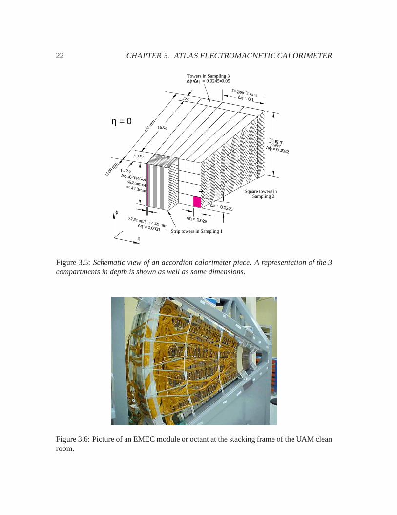
1.475) [17] and two end-caps (−3.2 < η < −1.375 , 1.375< η < 3.2) [18] and is seg-mented in depth in three compartments (see figure 3.5). Thereis also a thin presamplerdetector in front of the calorimeter covering the region|η| < 1.8, which task is to correctfor the energy losses of electrons and photons in the upstream material.

The Argon is kept liquid at a temperature of∼ 89oK through a cryogenic system,being the EM barrel and end-cap calorimeters inside their respective cryostat vessels.

3.3 End-cap specifities

There are two EMEC cylinders in ATLAS located inside the End-cap Cryostat atz∼±350 cm of the nominal interaction point. A picture of one EMECinside the End-Capcryostat can be seen in figure 3.4. Since the EMEC is a cylindrical wheel, the amplitudeof the accordion waves decreases whenη increases (when the radious decreases). Due tomechanical constraints demanded by this accordion shape, asecond independent wheel isneeded to extend the coverage toη = 3.2. Hence, there are two wheels, the outer wheelfrom η = 1.375 toη = 2.5 and the inner wheel fromη = 2.5 to η = 3.2. The lead iscladded by 0.2 mm thick steel to give it enough rigidity. For the outer wheel, the thicknessof the lead plates is 1.7 mm while the LAR gap thickness between the absorber and theelectrode decreases continuously from 2.8 mm (atη = 1.375) to 0.9 mm (atη = 2.5)whenη increases. For the inner wheel, the thickness of the lead plates is 2.2 mm while

3.3. END-CAP SPECIFITIES 21

the LAR gap thickness between the absorber and the electrodedecreases continuouslyfrom 3.1 mm (atη = 2.5) to 1.8 mm (atη = 3.2) whenη increases.

Figure 3.4: Picture of an EMEC wheel inside the End-Cap Cryostat.

To facilitate handling and logistics the EMEC cylinder is divided into 8 octants ormodules (see figure 3.6). The 16 modules have been stacked in the CPPM1 and UAM 2

clean rooms.

One module consists of 96 (32) layers for the outer (inner) wheel stacked one on topof each other. Each layer is a sandwich of absorber, spacer (gap), electrode, spacer (gap).The design is symmetrical inφ and projective to the interaction point inη. In particularthe cells drawn in the electrodes point to the nominal ATLAS interaction point.

1Centre de Physique des Particules de Marseille2Universidad Autonoma de Madrid


∆ϕ = 0.0245

∆η = 0.02537.5mm/8 = 4.69 mm ∆η = 0.0031

∆ϕ=0.0245x4 36.8mmx4 =147.3mm

Trigger Tower

TriggerTower∆ϕ = 0.0982

∆η = 0.1

16X0

4.3X0

2X0

1500

mm

470

mm

η

ϕ

η = 0

Strip towers in Sampling 1

Square towers in Sampling 2

1.7X0

Towers in Sampling 3 ∆ϕ×∆η = 0.0245×0.05

Figure 3.5:Schematic view of an accordion calorimeter piece. A representation of the 3compartments in depth is shown as well as some dimensions.

Figure 3.6: Picture of an EMEC module or octant at the stacking frame of the UAM cleanroom.

3.4. BARREL SPECIFITIES 23

3.4 Barrel specifities

The barrel electromagnetic calorimeter (EMB) is made of twohalf-barrels, centered aroundthe z-axis. One half-barrel covers the region 0< η < 1.475 and the other one the region−1.475< η < 0. The length of each half-barrel is 3.2 m, their inner and outer diametersare 2.8 m and 4 m respectively.

Figure 3.7: Diagram of a half of the EM Barrel.

Figure 3.7 shows a diagram of one half-barrel. The directionof the accordion wavesis indicated pointing to thez axis as well as the calorimeter cells which points to the AT-LAS center or nominal interaction point. The calorimeter isinside the cryostat vesselwhich has two walls, warm and cold, separated with a vacuum gap for temperature isola-tion purposes. The cables pass from inside to outside of the cryostat vessel using specialfeedthrough connectors which keeps the temperature isolation. In the ”warm” part (out-side the cryostat) crates are connected to the feedthroughs, which contains some electron-ics boards: Front End Boards (FEB) and Calibration Boards. It can also be seen in figure3.7 a tube on top of the cryostat through which the cryogenic system injects the liquidArgon.

The size of the LAR gap on each side of the electrode is 2.1 mm, which corresponds


to a total drift time of about 450 ns for an operation voltage of 2000 V. For ease ofconstruction, each half-barrel has been divided into 16 modules, each covering a∆φ =22.5o. A picture of one EMB module is shown in figure 3.8.

Figure 3.8: Picture of an EMB module.

3.5 Segmentation

The EM Calorimeter is segmented into cells along the two angular directions,η andφ,and the longitudinal direction (calorimeter depth). Alongthe calorimeter depth threecompartments are defined, by reading out three regions of theelectrode independently,namely: Front or S1, readout from the calorimeter front side, Middle or S2 and Back orS3, both readout from the calorimeter back side (see figure 3.5).

The granularity alongη is also defined in the electrodes as copper strips using kap-ton as electrical isolator between two strips. The size of such strips depends on the com-partment, being smallest in the S1 to allow for the separation of the two photons fromthe decay of aπ0. A picture of an EMEC electrode (outer wheel) is shown in figure 3.9.The angular variableη increases from right to left of the picture. The copper strips areclearly seen defining the granularity along theη direction. The three compartments indepth, S1, S2 and S3, can be clearly distinguished as the width of the strips changes fromone compartment to another.

The granularity along the azimuthalφ direction is defined by connecting summingboards to the electrode connectors, hence grouping the signal in φ. For example, for theS2 compartment of the EMEC, three consecutive electrodes are connected (are summed)

3.6. HIGH VOLTAGE 25

Figure 3.9: Picture of an EMEC electrode of the outer wheel. The segmentation alongηand the three compartments in depth, S1,S2 and S3, are clearly seen.

to obtain the desired granularity of∆φ = 0.025 radians, while 12 electrodes are connectedfor the S1 compartment of the EMEC given a granularity of∆φ = 0.1 radians in this com-partment. Figure 3.10 shows some summing boards plugged in the electrode connectorsfor the S1 compartment of an EMEC module. Theφ direction goes from bottom to topof the picture, while theη direction increases from left to right. The electrode connectorscan be distinguished in black between two absorbers. The summing boards grouped thesignals of 12 electrodes together in this example.

The electromagnetic calorimeter granularity is detailed in Table 3.1. In total thenumber of cells or channels in the electromagnetic calorimeter is∼ 170000 (101760 inbarrel, 62208 in end-caps and 9344 in presampler).

3.6 High Voltage

The High Voltage (HV) between the electrodes and absorbers is generated by some spe-cial HV units outside the cryostat. The HV thin cables pass through some dedicatedcryostat feedthroughs to reach the HV boards on the calorimeter. A picture of one EMECHV board is shown in figure 3.11. It is plugged into some dedicated connectors of theelectrodes. Theφ direction goes from left to right andη increases from top to bottom inthe figure. There is one column of HV boards alongφ-direction per high voltage value(per high voltage region).

The condition of projectivity to the nominal ATLAS interaction point in the con-


Figure 3.10: Picture the summing boards plugged in the frontface of an EMEC module.

Front (S1) Middle (S2) Back (S3)

|η| ≤ 1.35 0.025/8×0.1 0.025×0.025 0.050×0.025Barrel 1.35≤ |η| ≤ 1.4 0.025/8×0.1 0.025×0.025 –

1.4≤ |η| ≤ 1.475 0.025×0.025 0.075×0.025 –

1.375≤ |η| ≤ 1.425 0.050×0.1 0.050×0.025 –1.425≤ |η| ≤ 1.5 0.025×0.1 0.025×0.025 –1.5≤ |η| ≤ 1.8 0.025/8×0.1 0.025×0.025 0.050×0.025

End-caps 1.8≤ |η| ≤ 2.0 0.025/6×0.1 0.025×0.025 0.050×0.0252.0≤ |η| ≤ 2.4 0.025/4×0.1 0.025×0.025 0.050×0.0252.4≤ |η| ≤ 2.5 0.025×0.1 0.025×0.025 0.050×0.0252.5≤ |η| ≤ 3.2 0.1×0.1 0.1×0.1 –

Table 3.1:Granularity∆η×∆φ for each calorimeter sampling (Front, Middle and Back).

3.6. HIGH VOLTAGE 27

Figure 3.11: Picture of an EMEC HV board

struction of the EMEC makes that the Liquid Argon gap thickness (between absorber andelectrode) decreases continuously whenη increases. The relation between the energycollected by the calorimeter (E) and the liquid Argon gap thickness (g) is [6]:

E ∼ fsg1+bUb (3.1)

whereU is the High Voltage applied on the gaps andfs the sampling fraction3 (which isa function of the gap thickness).

The decrease of the liquid Argon gap thickness whenη increases implies an in-crease of the measured energy withη. This growth may be compensated by decreasingUcontinuously whenη increases. For practical reasons a decreasing stepwise function forU is chosen defining seven HV sectors for the outer wheel and twosectors for the innerwheel. The growth of the measured energy withη inside a HV sector is corrected bysoftware in the reconstruction phase of the signal, keepingthen the required uniformityof the calorimeter signal response.

In contrast, for the EM Barrel Calorimeter this problem doesnot occur and, as aconsequence, the High Voltage between electrodes and absorbers is kept constant, beingthe nominal value 2000 Volts.

The High-Voltage sector definitions, consequence of the end-cap geometry, is givenin Table 3.2.

3The sampling fraction is defined as the energy deposited in the LAR divided by the sum of the energydeposited in the Absorbers and the LAR.


Barrel End-cap Outer W. End-cap Inner W.

HV region 0 1 2 3 4 5 6 7 8 9

η range 0-1.475 1.375-1.5 1.5-1.6 1.6-1.8 1.8-2.0 2.0-2.1 2.1-2.3 2.3-2.5 2.5-2.8 2.8-3.2

HV values 2000 V 2500 V 2300 V 2100 V 1700 V 1500 V 1250 V 1000 V 2300 V 1800 V

Table 3.2:The high voltage regions of the EM calorimeter.

3.7 Electronics

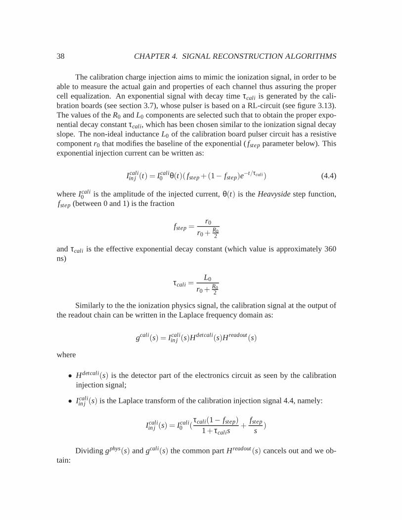
The electric signal from the ionization of the Liquid Argon produced by a charged particlehas a triangular shape, when representing the intensity versus time, with typical durationof several hundreds nano-seconds. This signal pass throughthe electrode readout pathsto the Summing Boards and the Mother Boards on top of them. Long cables connect theMother Boards to the electronics outside the cryostat. A picture of the Summing Boardscan be seen in figure 3.10 and of the Mother Boards in figure 3.12.

Figure 3.12: Picture of one Mother Board of the front side of the EMEC.

A simplified schematic view of the calorimeter readout is shown in figure 3.13.The detector cell is represented by a capacitanceC where a triangular ionization signal(I phys

in j (t)) is generated by the detected particle. Also linked to a cellthere appears aninductanceL due to the electrode, the Summing-Board and a small portion of the Mother-Board. The signal travels through a 25Ω cable in case of a middle or a back cell and a 50Ωcable in case of a front cell. Immediately after the feedthrough of the cryostat the signalenters a Front-End-Board (FEB) and pass through a three gainshaper with gain factors1, 9.3 and 93 corresponding to low, medium and high gain respectively. The measured

3.7. ELECTRONICS 29

shaped signalgphys(t) is sampled by a Switch Capacitor Array (SCA) located in the FEBat a frequency of 40 MHz (equivalent to a period of 25 ns), thatis the nominal bunchcrossing frequency of LHC beams. The samples are digitized by ADCs located in theFEB and the numbers are transmitted to the miniROD and the DAQcomputing system inthe control room (see figure 3.14).

Figure 3.13: Diagram of the EM calorimeter readout inside the detector.

A diagram of one calibration line is also shown in figure 3.13.An exponential signal(I cali

in j (t)) is generated in the Calibration Board playing the role of the triangular ionization

signal (Ip) of physics events. The signalI caliin j pass the feedthrough to get into the cryostat


and travels through a long cable up to the Mother-Board. The calibration signal sees thedetector cell as a capacitance and an inductance as indicated in figure 3.13. The responseto this injection signal continues through the same readoutline as the ionization signal toreach the SCA. The output is again seven samples of the shapedsignalgcali(t) after beingdigitized by the ADC.

The calibration boards allow to set the amplitude of injected currentI caliin j numer-

ically. A DAC unit, included in the calibration board, transforms this number into ananalog amplitude. We will refer to this number as DAC value. The calibration board isequipped with a delay unit, which allows to delay the injection from 0 to 24 ns in steps of1 ns with respect to the leading edge of the 40 MHz clock (tdelay). The calibration pulsegcali(t) is obtained by representing the sample heights as a functionof tdelay. 4. Thesedelay runs were taken inbetween cosmic runs. Delay runs in high (medium, low) gainwith a DAC value of 500 (4000,40000) units are considered forthe signal reconstructionstudies.

3.8 Some differences between EMEC and EMB

Some differences between EMEC and EMB relevant to the study of this document aresummarized in table 3.3.

Barrel End-caps (outer wheel)

Gap (absorber-electrode) (mm) 2.1 3.1 to 0.9Bending angle () 70 to 90 60 to 120

Drift time (ns) 470 600 to 200dE/dX sampling fraction (%) 25 or 28 30 to 14

HV (V) 2000 2500 to 1000

S2 Cell inductanceL (nH) 25 to 35 50 to 20S2 Cell Capacitance at coldC (pF) 1400 or 1900 1200 to 600

Table 3.3:Some geometrical and electrical characteristics of the barrel and end-cap outerwheel EM calorimeter. In the former case, parameters may vary at |η|= 0.8. In the lattercase, the variation is smooth and given for increasing|η| from 0 to 2.5.

4Every sample height is an average over 100 events taken for a given delay

3.8. SOME DIFFERENCES BETWEEN EMEC AND EMB 31

Figure 3.14: Diagram of the EM calorimeter readout


Chapter 4

Signal Reconstruction Algorithms

The ATLAS Liquid Argon electromagnetic calorimeter uses a digital filtering technique,called Optimal Filtering Method, to reconstruct the signalamplitude from samplings ofthe ionization pulse. Some weights, optimal filtering coefficients, are determined fromthe pulse shape and its derivative, such that the weighting sum of the samplings givesthe amplitude of the signal per cell. Each read-out channel can be calibrated by means ofelectronic pulses that mimic the ionization signal produced by an electromagnetic shower.The calibration and the ionization signal are different in shape (exponential/triangular,respectively) and injection point (outside/inside the detector). It is necessary to know theelectrical parameters of every cell in the detector to deduce the ionization signal using thecalibration signal.

This chapter gives a brief description of the Optimal Filtering Method, the detectormodel, the prediction of the ionization signal from the calibration signal and an algorithmto determine the electrical parameters of the calorimeter cell.

4.1 Optimal filtering method

The LAr EMC signal is generated by the drift of the ionizationelectrons in the electricfield provided by the High Voltage (HV) in the LAr gap. The current versus time hasa triangular shape, being the peak proportional to the energy deposited by the electro-magnetic shower. The ionization signal is pre-amplified andthen shaped by aCR−RC2

bipolar filter at the end of the readout chain. The bipolar signal is sampled every 25 ns(the LHC bunch crossing period) and 5 samples are digitized and used in the signal re-construction procedure. For special runs more than 5 samples are digitized and recorded(typically 25 or 32). Figure 4.1 shows a comparison between the original triangular signalgenerated inside the LAr gap and the output signal after passing the readout electronics.

33

34 CHAPTER 4. SIGNAL RECONSTRUCTION ALGORITHMS

It corresponds to a cell of theS2 compartment for medium gain of the bipolar shaper. Themaximum has been normalized to 1. The bipolar shaper is designed such that the max-imum of the triangular signal corresponds to the maximum of the shaped pulse. Hence,the maximum amplitude of the shaped pulse is proportional tothe energy deposited bythe electromagnetic shower in thatS2 cell. The dots correspond to the samples each 25ns.

Figure 4.1: The triangle shape corresponds to the signal as afunction of time just afterthe electrode, and the bell shape corresponds to the signal after crossing the shaper. Dotsrepresent the recorded amplitudes separated by 25 ns.

From these samples two relevant quantities are deduced, using a digital filteringtechnique, namely the signal maximum amplitude (Amax), which is proportional to theenergy deposited in the cell, and the time shift (∆t) of the signal maximum amplitudewith respect to a reference value. The Optimal Filtering (OF) method is a digital filteringtechnique to determine such quantities. The inputs to the method are: i) the covarianceor autocorrelation matrix of the samples, which contains the information of the noise, ii)the pulse shape (gphys), its maximum normalized to one, ii) and its derivative (dgphys/dt).The outputs of the method are some weights or coefficients,ai, bi i = 1, . . . ,n, wheren isthe number of samples, such that:

Amax=n

∑i=1

aiSi (4.1)

∆t =∑n

i=1biSi

Amax(4.2)

beingSi i = 1, . . . ,n the measured samples (pedestal or zero is subtracted).

4.1. OPTIMAL FILTERING METHOD 35

The Optimal Filtering coefficients (OFC),ai , bi i = 1, . . . ,n, are calculated by themethod with the condition to minimize the noise contribution to the signal [19].

Two sources of noise are foreseen in the calorimeter during operation at LHC:

• Thermal (or electronic) noise

The amplitude of the thermal noise depends only upon the characteristics of thedetector and the signal processing circuitry.

• Pile-up (or physics) noise

The minimum bias or soft scattering events will be superimposed to the hard scat-tering process. It is expected to have about 27 minimum bias events per bunchcrossing at nominal LHC luminosity. In addition, events of previous bunch cross-ings will affect the signal of the present crossing, since the ionization time constantof the liquid Argon is several hundred nano-seconds. The overall effect is a smallsignal in the cells, fluctuating from event to event, which can be considered asa noise superimposed to the hard process physics event of interest. The level ofpileup noise depends therefore on the luminosity of the machine and on the size ofthe calorimeter cells.

Since the present work refers to cosmics muon data, only the first source of noiseenters in the analysis. In future, for the analysis of the LHCdata we will need to take thepile-up noise contribution into account as well.

In ATLAS, where the bunch crossings and the readout clock aresynchronous thepulses get always sampled at the same position and one set of OFC is sufficient. However,in the cosmic test environment this is not the case since the cosmic signal is asynchronousto the readout clock. Depending on the phase shift between the clock and the particlearrival, a different fraction of the pulse is sampled. To cope with this situation, multiplesets of OF coefficients are calculated dividing the 25nsregion between two ADC samplesin bins of ∆t ∽ 1 ns. For the present analysis, a set of(ai ,bi), i = 1, . . . ,n coefficientsfor each time phase has been calculated, up to a total of 50 phases in 1ns steps and forhigh gain. Medium and low gains are not used since most of the muons deposit an energylower than 20 GeV in the EM Calorimeter. The fact of duplicating the number of phasesin the analysis, 50 instead of 25, allows to perform cross-checks at different timings andguarantees to cover completely the 25nsregion of interest.

4.1.1 Prediction of physics pulse

As seen in the previous section, the pulse shape of the ionization (or physics) signal isneeded to determine the Optimal Filtering Coefficients for each calorimeter cell. However


L

C

read-out line

r CR-RC2

I ionI cali

Hr.o.

Figure 4.2:Schematic electrical model of a LAr cell with its readout chain and calibrationnetwork. Shapes of calibration and ionization signals are illustrated, as well as the outputpulse.

this shape is unknown and must be predicted either by a complete description of thereadout chain or from the corresponding calibration pulse shape and a few parameters(due to the differences between the ionization signal and the calibration signal). Thesecond procedure has been adopted in this work.

Although the readout path and electronics is the same for physics and calibrationinputs, there are two differences at the injection point, namely:

• the physics input signal is produced inside a gap of the detector, while the calibra-tion input is generated outside the cryostat in a calibration board connected on aFront End Crate. This difference makes the calibration see the calorimeter cell as adifferentrLC circuit.

• the physics input signal has a triangular shape when represented as a function oftime, while the calibration charge injection has an exponential shape.

In figure 4.2 a simplified diagram of the electrical model for aLAr cell is shown.The calorimeter cell is seen as anrLC circuit: the capacitanceC of the LAr gap, aninductanceL which has two contributions, one from the electrode path between the gapand the Summing Board and the other one from the path inside the Summing Board itselfadded to a small portion of Mother Board, and a small resistance r of the total path.The injection point of the ionization (physics) and calibration signals is indicated as well.Clearly these signals see the cellrLC circuit in a different way,rL in parallel withC forphysics injection signal and in serial in the case of calibration. The different shapes ofthe injection current between physics and calibration (triangular and exponential) is alsoshown.

4.1. OPTIMAL FILTERING METHOD 37

The ionization electrons drift in the electric field inside the LAr gap, producing acurrent with amplitude proportional to the released energy. This current has the typicalionization-chamber triangular shape, with a rise time of the order of 1 ns followed by alinear decay for the duration of the maximum drift timetdri f t . Such a signal at the inputof the cell capacitor in time domain is given by:

I physin j (t) = I phys

0 θ(t)θ(tdri f t − t)(1− ttdri f t

) (4.3)

whereθ is theHeavysidefunction andI phys0 is the amplitude of the ionization current. The

drift time tdri f t in a 2 mm gap under a voltage of 2000 V is close to 400 ns. This time is afunction of the pseudorapidity for the EMEC due to the changein the LAr gap and in thevoltage, taking values in the range 200-600 ns.

The output physics signal can be written as:

gphys(t) =

Z +∞

−∞Kp(t− t ′)I phys

in j (t ′)dt′

whereKp contains the information of the readout circuitry.

In the Laplace domain (applying the “Convolution Theorem”), we find:

gphys(s) = I physin j (s)Kp(s)

where:

• Kp(s) can be written as the product of a factorHdet(s), which contains the electron-ics characteristics related to a detector cell (rLC circuit), and a factorHreadout(s),which takes into account the readout chain (common for physics and calibrationsignals);

• I physin j (s) is the injected ionization signal 4.3 in the Laplace frequency domain, that

is:

I physin j (s) = I phys

0 (1

tdri f ts− 1−e−tdri f t s

t2dri f t s

2)

Hence, the output physics signal can be written as:

gphys(s) = I physin j (s)Hdet(s)Hreadout(s)


The calibration charge injection aims to mimic the ionization signal, in order to beable to measure the actual gain and properties of each channel thus assuring the propercell equalization. An exponential signal with decay timeτcali is generated by the cali-bration boards (see section 3.7), whose pulser is based on a RL-circuit (see figure 3.13).The values of theR0 andL0 components are selected such that to obtain the proper expo-nential decay constantτcali, which has been chosen similar to the ionization signal decayslope. The non-ideal inductanceL0 of the calibration board pulser circuit has a resistivecomponentr0 that modifies the baseline of the exponential (fstepparameter below). Thisexponential injection current can be written as:

I caliin j (t) = I cali

0 θ(t)( fstep+(1− fstep)e−t/τcali) (4.4)

whereI cali0 is the amplitude of the injected current,θ(t) is theHeavysidestep function,

fstep(between 0 and 1) is the fraction

fstep=r0

r0+ R02

andτcali is the effective exponential decay constant (which value isapproximately 360ns)

τcali =L0

r0 + R02

Similarly to the the ionization physics signal, the calibration signal at the output ofthe readout chain can be written in the Laplace frequency domain as:

gcali(s) = I caliin j (s)Hdetcali(s)Hreadout(s)

where

• Hdetcali(s) is the detector part of the electronics circuit as seen by thecalibrationinjection signal;

• I caliin j (s) is the Laplace transform of the calibration injection signal 4.4, namely:

I caliin j (s) = I cali

0 (τcali(1− fstep)

1+ τcalis+

fstep

s)

Dividing gphys(s) andgcali(s) the common partHreadout(s) cancels out and we ob-tain:

4.2. COMPUTATION OFGPHYS 39

gphys(s)gcali(s)

=I phys0

I cali0

Hdet(s)Hdetcali(s)

Hence, the physics signal or physics pulse shape can be obtain from the calibrationpulse shape through the following expression in the Laplacefrequency domain:

gphys(s) = gcali(s)I physin j (s)

I caliin j (s)

Hdet(s)Hdetcali(s)

Or in the time domain as:

gphys(t) =

[

gcali ×L−1

(

I physin j (s)

I caliin j (s)

)

×L−1(

Hdet(s)

Hdetcali(s)

)

]

(t) (4.5)

where× means convolution.

The second and third factors in the convolution take into account the differences inthe injection signal and injection point respectively between the physics and the calibra-tion signals.

4.2 Computation ofgphys

For computational purposes the relation 4.5 can be written as:

gphys(t) =

[

gcali ×L−1(

(1+sτcali)(stdri f t −1+e−stdri f t )

stdri f t ( fstep+sτcali)

)

×L−1(

11+s2LC+srC

)]

(t)

=[

gcali×gexp→tri ×gMB→det]

(t) (4.6)

where the two different time-domain convolutions are:

gexp→tri(t) = δ(t)+

[

1− fstep

τcalie− fstep

tτcali − 1− fstep

fstep

(

e− fstep

tτcali −1

)

]

θ(t)

+1− fstep

fstep

(

e− fstep

t−tdri f tτcali

)

θ(t −Td)


gMB→det(t) =2τa

e(τr/(2τ20))tθ(t)

whereτr = rC andτ0 = LC.

The procedure requires the knowledge of the calibration pulsegcali (see chapters3 and 7) and of a set of five parameters, namely two related to the calibration board,τcali and fstep, two related to the cell electrical properties,τ0 andτr , and one related tothe ionization,tdri f t . Their values may depend on the detector conditions, temperature,radiation dose, etc, hence it is important to monitor them ona regular basis. The parametertdri f t has been measured at the beam tests, while the other four parameters can be extractedeither from direct measurements or from the calibration pulse using the algorithm calledResponse Transformation Method (RTM)

4.3 Parameter extraction algorithm (RTM)

The RTM method was developed by the Milan Atlas group to be applied to the Barrel EMcalorimeter [11]. The method consists in the following. We have seen that the responseto a calibration injection pulse can be expressed in the Laplace frequency domain as:

gcali(s) = I caliin j (s)Hdetcali(s)Hreadout(s)

The functionHdetcali(s) describes the effects of the detector cell properties on thein-jected calibration signalI cali

in j (s), whileHreadout(s) is the readout (line+preamplifier+shaper)transfer function.

Let a generic current pulseYin j(s) be injected on the system at the Mother Boardlevel, as it is actually done with the real calibration pulseI cali

in j (s). The responseWout(s) ofthe system to this signal would be:

Wout(s) = Yin j(s) Hdetcali(s) Hreadout(s) =Yin j(s)

I caliin j (s)

I caliin j (s) Hdetcali(s) Hreadout(s) =

=Yin j(s)

I caliin j (s)

gcali(s)

or, in the time domain:

Wout(t) =

[

gcali×L−1

(

Yin j(s)

I caliin j (s)

)]

(t)

4.3. PARAMETER EXTRACTION ALGORITHM (RTM) 41

The dependence on the circuit parameters has cancels out andonly remains the ratiobetween the different injection functions.

The RTM bases its strategy to retrieve parameters on the computation and analysisof what would be the response to a signal different from the ”exponential” calibrationinjection signal. The system response can in fact be sensitive to a particular injectedwaveform, the output showing in some cases easily recognizable characteristics. In thefollowing steps, waveforms will be sought that minimize thesignal tail ofWout(t). Forthis purpose, aχ2-like quantity is built by summing the squares of the values of Wout(t)along the tail, that is:

Q2 = ∑t>ttail

W2out(t)

the tail being defined as the signal portion after the timettail .

In particular, to obtain the calibration board parameters,τcali and fstep, a step func-tion will be chosen forYin j(t), and to extractτ0 a cosine function forYin j(t) is moresuitable.

Extraction of the calibration boards parameters: τcali and fstep

To obtain the calibration pulse parametersτcali and fstep a step function,Yin j(t) = θ(t),is used with unit amplitude. The Laplace transform of the step function isYin j(s) = 1/s.On the other hand, the expression forI cali

in j (s), seen in previous section, can be written, forunit amplitude, as:

I caliin j (s) =

τ′calis+ f ′step

s(1+ τ′calis)

Hence, the ratio between both injection signals is:

Yin j(s)

I caliin j (s)

==1+sτ′cali

sτ′cali + f ′step

andWout can be obtained as:

Wout(s) =1+sτ′cali

sτ′cali + f ′stepgcali(s)

It can be shown that, for the correct valuesτ′cali = τcali and f ′step= fstep of thecalibration board parameters,Wout(t) has the property of going to zero in the tail very


rapidly. This is due to the fact that bothHdet andHreadout functions contain only shorttime constants and do not give rise to a long tail in the waveform.

This null-tail property of the step-response can be used to determine both calibrationboard parameters by minimizing the following quantity:

Q2(τ′cali; f ′step) = ∑t>ttail

W2out(t;τ′cali; f ′step)

The minimization procedure may in principle depend on the tail starting point valuettail . A robust choice ofttail is given byttail = tmin+ 100ns, wheretmin is the minimumof the negative lobe of the shaped signal1. Using this criterion the systematic errorintroduced byttail in the RTM procedure is small.

Extraction of the detector parameters: τ0 and τr

To extractτ0, or equivalentlyω0 = 1/τ0, the response to a monochromatic cosine pulseYin j(t) = θ(t)cos(ωt) is studied, which, in the Laplace frequency domain, has the form:

Yin j(s) =s

s2+ω2

The ratio between both ”cosine-type” and calibration injection signals is:

Yin j(s)

I caliin j (s)

==s

s2+ω2

s(1+sτcali)

sτcali + fstep

andWout can be obtained as:

Wout(s) =s

s2+ω2

s(1+sτcali)

sτcali + fstepgcali(s)

It turns out that the smallest amplitude for this function isobtained whenω = ω0,hence this parameter is obtain by minimizing the following quantity:

Q2(ω) = ∑t>ttail

W2out(t;ω)× (1+(ωτsh)

2)3

(ωτsh)2

1One can look at figure 4.1 to see the negative lobe of the shape signal, although the pulse shape corre-sponds to a ionization signal instead of a calibration step function

4.3. PARAMETER EXTRACTION ALGORITHM (RTM) 43

where the last term introduces a shaper correction in this case, due to the fact that theshaper acts as a band-pass filter suppressing the high frequency components of the injectedsignals.

Finally the parameterτr can be extracted by injectingYin j = I caliin j , however at the

physics injection point. This introduces a correction factor in the output signal, whichdepends onτ′r as follows:

11+sτ′r +s2τ′0

Hence,

Wout(s) =1

1+sτ′r +s2τ′0gcali(s)

If τ′0 6= τ0 or τ′r 6= τr the functionWout(t) will have an oscillating behavior on thetail. We can assume thatτ0 has been obtained before by the RTM method, as described inprevious subsection, or by direct measurements. Hence, thequantity to minimize in orderto obtainτr is defined as:

Q2(τ′r) = ∑t>ttail

(Wout(t;τ′r)−gcali(t))2


Chapter 5

Signal reconstruction in the end-caps

The first section of this chapter synthesizes the present knowledge of the input parametersneeded to compute the optimal filtering coefficients for the end-caps. As a first cross-check, and wherever it is relevant, these inputs are compared to the EM barrel ones.The outputs of the method,i.e. the predicted physics pulse shapes, the optimal filteringcoefficients, the calibration bias and the noise reduction,are discussed in section 5.2.

5.1 Inputs for the end-caps

5.1.1 Cell response to a calibration signal

Typical shapes of cell responses to a same calibration inputare shown in Figure 5.1 (left)for the three EMEC layers. The differences between shapes are explained by the elec-trical characteristics of each layer. Notice that, in the finely segmented part of the frontsampling, 1.5< η < 2.4, the crosstalk between neighbor cells is important, between 3 and5% [21], and has been taken into account by adding the two neighboring cell shapes to thepulsed one. As a global sanity check, the dispersion alongφ of the maximum amplitudeof all calibration shapes is shown to be the same for all layers and exhibits no dependencyas a function ofη (Figure 5.1, right).

45

46 CHAPTER 5. SIGNAL RECONSTRUCTION IN THE END-CAPS

Time (ns)0 200 400 600 800

A (

AD

C)

0

1000

2000

S1

S2

S3

η1.4 1.6 1.8 2 2.2 2.4 2.6 2.8 3 3.2

/mea

nσ

0

0.005

0.01

0.015

0.02

0.025

0.03

0.035

Figure 5.1:Left: Typical calibration pulse shapes atη = 1.8 for an input of 500 DACunits in high gain. Right: Dispersion overφ of the maximum amplitude of all calibrationshapes in high gain, as a function ofη. Front, middle and back cells are represented withred down triangles, black squares and blue up triangles, respectively.

5.1.2 Calibration board parameters

To obtain an efficient calibration, the input signal should be as similar as possible to theionization triangular pulse. Two main parameters,τcali and fstep, are needed to describethis calibration input pulse:

I caliin j (t) = I cali

0 ·θ(t) ·[

(1− fstep)e− t

τcali + fstep

]

(5.1)

whereθ(t) is the unit step function. The exponential decay timeτcali is chosen to mimicthe decay slope of the ionization signal, whilefstep is related to the resistive componentof the inductance in the calibration board [11].

These two parameters need to be known for every calibration board channel. Theycan be extracted from measurements in the production laboratories [22] or can be inferredfrom the cell response to a calibration pulse using the Response Transformation Method(RTM) [11]. Figure 5.2 shows a comparison between the two methods for both parame-ters of one calibration board. Relative systematic shifts of −7% and+15% using RTMcompared to the measured values are observed for extractedτcali and fstep, respectively,which is as expected in very good agreement with what was already reported for the bar-rel. This is probably because RTM gives effective parameters, absorbing for instanceattenuation effects [23, 24]. As not all calibration board measurements were available,the RTM extracted parameters are chosen to be consistent. Notice that choosing the RTMextracted parameters impacts only the absolute energy scale, which can not be tested veryprecisely with cosmic data.

5.1. INPUTS FOR THE END-CAPS 47

Channel0 20 40 60 80 100 120

(n

s)ca

liτ

370

380

390

400

410

420

430

440

450

460

Channel0 20 40 60 80 100 120

step

f

0.065

0.07

0.075

0.08

0.085

0.09

0.095

0.1

Figure 5.2:Comparison ofτcali (left) and fstep (right) extracted by RTM (open symbols)and measured directly (closed symbols) for the 128 channelsof one calibration board.

5.1.3 Ion drift time in liquid argon gap

The ion drift time in liquid argon gap,tdri f t , can be expressed in terms of applied highvoltageU and gap thicknessg [26]:

tdri f t =g

Vdri f t∼ gb+1

Ub (5.2)

whereb∼ 0.4 is a parameter first determined with specific measurements [26] and thencrosschecked with beam tests [27, 28, 29]. As indicated in section 3.2, the complicatedEMEC geometry implies a variation of the gap thickness alongη, which induces a vary-ing drift time despite the change in the high voltage. This isa major difference with thebarrel part, for which the drift time is almost constant around 470 ns forU = 2000 V.

The drift time can be computed using Equation (5.2) or extracted from a fit to thephysic pulse shapes recorded with test-beam data1 [28], with a precision estimated around10%. Figure 5.3 shows the measuredtdri f t , averaged overφ, as a function ofη for allEMEC layers2. They are in good agreement with the predictions extracted from Equa-tion (5.2). Notice that any change on HV setting conditions implies a change of the drifttime in the corresponding region.

1At the beam tests, as events are asynchronous with respect tothe clock, the 5 sample physics pulse ina cell can be averaged within a 1 ns bin by using the phase of each event.

2No measurement was available in the region 1.4< |η|< 1.6, in which the prediction is therefore taken.


η1.4 1.6 1.8 2 2.2 2.4 2.6 2.8 3 3.2

(ns)

drift

t

150

200

250

300

350

400

450

500

550

600

650

Figure 5.3: Drift time as a function ofη for front (red down triangles), middle (blacksquares) and back (blue up triangles) end-cap layers. All points have been averaged overφ.

5.1.4 Electronic chain characteristics

A thorough program of measurements was carried out at cold onall cells of the EMECcalorimeter before installation of the front end electronics to measure their electrical prop-erties as precisely as possible. By means of a Network Analyser [22], a frequency scanwas performed to extract precisely the resonance frequencyof the cell circuitω0 = 2πν0 =1/τ0 = 1/

√LC and the productτr = rC. In both cases, the most precise measurements

were obtained in the second layer (first layer in the inner wheel), where capacitances arehigher. Results are more difficult or impossible to extract in the first and third layers, andthe approximationτ0 = τr = 0 is therefore used in the following for these samplings.

Resonance frequency

Typical examples of end-cap S2 cell responses to a frequencyscan with a NetworkAnalyser are shown in Figure 5.4 (top). The resonance frequency is clearly visible on theleft-hand plot, and is obtained by fitting a parabola around the minimum. The determi-nation of the resonance frequency can be complicated by the presence of reflections nearthe peak, as illustrated in the second column of Figure 5.4 (top). This situation is evenmore pronounced when the resonance frequency is higher,i.e. the capacitance and theinductance are low, as for example at highη in the EMEC outer wheel (fourth columnof Figure 5.4 top). In the last two cases, the resonance frequency is inferred by fittingthe edges of the two minima with straight lines and computingthe intercept point of both


lines. To partly overcome this problem,ω0 is not measured for every cells but averagedoverφ at everyη. Results are shown in Figure 5.5 (closed symbols). Theirη-dependency,qualitatively reproduced by individual measurements ofL andC [30], reflects the decreaseof L andC as a function ofη. This has to be compared to the barrel case, with aω0 vary-ing only between 0.13 and 0.19 GHz [22].

(GHz)ω0.1 0.15 0.2 0.25 0.3

Tran

sfe

r F

un

c. (d

B)

-70

-60

-50

-40

=0.163 GHz0ω

(GHz)ω0.1 0.15 0.2 0.25 0.3

-70

-60

-50

-40

=0.165 GHz0ω

(GHz)ω0.1 0.15 0.2 0.25 0.3

-70

-60

-50

-40

=0.189 GHz0ω

(GHz)ω0.1 0.15 0.2 0.25 0.3

-70

-60

-50

-40

=0.242 GHz0ω

(GHz)ω0.1 0.15 0.2 0.25 0.3

arb

itrary u

nit

s

15

20

=0.173 GHz0ω

(GHz)ω0.1 0.15 0.2 0.25 0.3

15

20

=0.172 GHz0ω

(GHz)ω0.1 0.15 0.2 0.25 0.3

15

20

=0.227 GHz0ω

(GHz)ω0.1 0.15 0.2 0.25 0.3

15

20

=0.242 GHz0ω

Figure 5.4:Typical S2 cell responses in the 100-300 MHz frequency rangeat η = 1.6 (firstrow), η = 1.7 (second row),η = 1.8 (third row) andη = 2.2 (fourth row), as measuredwith a network analyser (top) and with the RTM method (bottom).

Because of the uncertainties in the resonance frequency measurement describedabove, it is desirable to extractω0 with an alternative method,i.e. RTM in this case. Thecorresponding output functions3 are illustrated for the same cells as for the measurementsin Figure 5.4 (bottom). In all cases, comparable results with measurements are obtained,apart in the third column where the resonance frequency is 20% higher. Figure 5.5 showsRTM and measurement results as a function ofη in S2. The agreement is good in theregions with high capacitances (η < 1.7 andη > 2.5), close to the barrel situation4. Thesituation worsens in the regions with lower capacitances,i.e. 1.7 < η < 2.5, where thedisagreement between RTM and measurements can reach up to 10-15%. To study thesystematic effect on energy measurement linked to this disagreement, the two differentω0 sets are considered in the following. Results are presentedin details in section 7.2.3.

3The resonance frequency corresponds to the minimum of the function.4The agreement between measurements and RTM extracted values at combined test-beam was∼ 1%

for S2, well compatible with the precision required [14].


η1.4 1.6 1.8 2 2.2 2.4 2.6 2.8 3 3.2

(GH

z)0ω

0.1

0.12

0.14

0.16

0.18

0.2

0.22

0.24

0.26

0.28

0.3

0.32

Figure 5.5:Cell resonance frequencyω0 obtained with network analyser measurements(closed symbols) and extracted with RTM (open dots), as a function ofη for S2 cells (S1in inner wheel). All points have been averaged overφ.

rC measurement

The productτr = rC can be determined by measuringr andC separately. Thervalues can be extracted from the frequency scan measurements by looking at the pulseamplitude at the resonance frequency [22], whereasC can be taken from direct mea-surements performed after EMEC module stacking [30]. Figure 5.6 shows theτr valuesobtained by this method as a function ofη. As for the resonance frequency, it is desirableto compare these measurements with the values extracted by RTM : a large disagreementis obtained, with measurements lower than RTM values by a factor∼ 5 (Figure 5.6). Thisis because RTM gives effective parameters,i.e. absorb some additional effects not con-sidered in the LAr readout model [25]. Similar observationsare made in the barrel, with afactor between RTM and measurements of∼ 2−3 [32]. However, the impact on the am-plitude determination is very small [11], and the measurements can not be used to predictthe physics shapes, as it generates residual oscillations in the tails [25]. This is illustratedin Figure 5.7 in the end-cap case, and is similar for the barrel. As a consequence, RTMextracted values will be used in the following.


η1.4 1.6 1.8 2 2.2 2.4 2.6 2.8 3 3.2

(ns)

rτ

0

0.5

1

1.5

2

2.5

3

3.5

4

4.5

5

Figure 5.6:Comparison of cellτr computed from the product of the measured r and C(open symbols) and extracted with RTM (closed symbols), as afunction ofη for S2 cells(S1 in inner wheel). All points have been averaged overφ.

Time (ns)0 200 400 600 800

A (

a.u

.)

0

0.5

1

Time (ns)0 200 400 600 800

A (

a.u

.)

0

0.5

1

Figure 5.7:Typical predicted physics pulse shape computed with measuredτr (left) andRTMτr (right) at η = 1.8.


5.1.5 Summary of the inputs

Excepttdri f t , all input parameters for signal reconstruction in the end-caps have been ei-ther directly measured or inferred from calibration systemthrough RTM method. Thechoice made between both has been discussed in the previous sections. The situation isvery similar to the barrel case for the calibration board parametersfstepandτcali, as well asfor τr . It is different forω0 in the regions with a high resonance frequency (1.7< η < 2.5),which renders the measurement difficult. To estimate the impact of a mismeasurement ofthis parameter, two sets of input parameters are considered, which can further serve toestimate the related systematic uncertainties on signal reconstruction (section 7.2.3). Ta-ble 5.1 summarizes the origin of the input parameters used topredict the physics pulseshapes in the end-caps. Theω0 set coming from direct measurements will serve as refer-ence in the following, and therefore used unless otherwise stated.

Outer Wheel Inner WheelParameter S1 S2 S3 S1 S2

fstep RTM RTM RTM RTM RTMτcali RTM RTM RTM RTM RTMtdri f t meas. meas. meas. meas. meas.

τr 0 RTM 0 RTM 0ω0 - Reference 0 meas. 0 meas. 0

ω0 - Set 2 0 RTM 0 RTM 0

Table 5.1: Origin of input parameters used for signal reconstruction in the end-caps.RTM refers to the Response Transformation Method [11], which infers the parametersfrom the cell response to a calibration pulse. Meas. refers to extensive measurementsperformed before the installation of the front end electronics. The twoω0 sets will beused to compute the two sets of optimal filtering coefficientslater tested in the cosmicmuon run analysis (section 7).

5.2. OUTPUTS OF THE METHOD 53

5.2 Outputs of the method

5.2.1 Computation of the pulse shapes and optimal filtering coeffi-cients for physics

All input parameters discussed in section 5.1 enter directly in Equation (4.6) to predict thephysics pulse shape of each EMEC cell. Typical shapes can be seen in Figure 5.8 (left) forthe three EMEC layers. As a first check on the quality of this prediction, the dispersionalongφ of the maximum amplitude is shown as a function ofη for the three layers inFigure 5.8 (right). It is roughly constant below 0.1% for S1 and S3 in the precision region(1.5 < |η| < 2.5). It decreases withη in S2, following theτ0 variation5. Notice thatthe same results are obtained with the twoω0 input sets of Table 5.1. More quantitativechecks of the quality of these predicted shapes are proposedin section 7.2.2 using cosmicdata.

Time (ns)0 200 400 600 800

A (

a.u

.)

0

0.5

1 S1

S2

S3

η1.4 1.6 1.8 2 2.2 2.4 2.6 2.8 3 3.2

/mea

nσ

0

0.001

0.002

0.003

0.004

0.005

0.006

0.007

0.008

0.009

0.01

Figure 5.8:Left: Typical predicted physics shape atη = 1.8 in high gain. Right: Disper-sion overφ of the maximum amplitude of all physics shapes in high gain, as a function ofη. Front, middle and back cells are represented with red down triangles, black squaresand blue up triangles.

From these physics pulse shapes and their derivatives, optimal filtering coefficients(OFC)ai andbi are computed per cell for each gain and for 50 phases by 1 ns step. Thishas been done with 5 or 25 samples and using one of the two inputparameter sets ofTable 5.1. Unless otherwise stated, the case with 5 samples and reference input set is usedin the following.

5It was checked that usingτ0 = τr = 0 in S2, results become similar to S1 and S3.


5.2.2 Estimation of the calibration bias

The difference between physics and calibration shapes induces a different response ampli-tude to a normalized input signal. The resulting bias must betaken into account in orderto correctly convert ADC counts into energy. This is achieved by using the ratio betweenthe maximum amplitudes of physics and calibration pulses, called

MphysMcali

. It is shown in

Figure 5.9 as a function ofη for the 3 EMEC layers in high gain6. The decreasing behav-ior with η reflects at first order the cell inductance variation [30] (mainly visible for S2),and at second order the drift time variation (visible for S1 and S3 where the inductance isassumed to be zero,τ0 = τr = 0).

η1.4 1.6 1.8 2 2.2 2.4 2.6 2.8 3 3.2

cali

/Mph

ysM

0.95

1

1.05

1.1

1.15

Figure 5.9:Bias in the signal reconstruction methodMphysMcali

in front (red down triangles),middle (black squares) and back (blue up triangles) EMEC cells. All points have beenaveraged overφ. High gain and the reference input set of Table 5.1 are used.

A comparison withMphysMcali

values obtained with 2001-2002 test beam analysis [13]is proposed in Figure 5.10 (left). The differences are quiteimportant, at the level of5−8% in the region 1.5 < η < 2.4, reflecting the different conditions of both analysesand data takings : cable lengths, optimal filtering coefficient computations, calibrationand front-end electronics, etc. As a systematic check, it isinteresting to make the samecomparison between the twoω0 input sets of Table 5.1. The agreement is at the percentlevel, as shown in Figure 5.10 (right). Finally, notice thatthe prediction of this bias on thesignal reconstruction method can hardly be checked with commissioning data, since theabsolute muon energy scale is only known at∼ 5% [15]. The uncertainties on

MphysMcali

ratio

6It was checked that the gain has no impact on the ratio.


will later be absorbed in the inter-calibration coefficients extracted with electrons fromZdecay [31].

η1.6 1.8 2 2.2 2.4

Ref

)ca

li/M

ph

ys(M

TB

)ca

li/M

ph

ys(M

1

1.03

1.06

1.09

1.12

1.15

η1.6 1.8 2 2.2 2.4

Ref

)ca

li/M

ph

ys(M

RT

M)

cali

/Mp

hys

(M

0.98

0.99

1

1.01

1.02

Figure 5.10:Ratios ofMphysMcali

in S2 between the present analysis with the reference set and2001-2002 test beam analysis [28] (left) and between the twoω0 input sets of Table 5.1(right).

5.2.3 Noise reduction with optimal filtering technique

The computation of the optimal filtering coefficients (OFC) is performed to minimize thenoise contribution to the signal reconstruction. To check this noise reduction, the OFC areapplied to pedestal runs for different number of samples. The noise level obtained using5 samples in high gain, averaged overφ, is shown in Figure 5.11 for the three EMEClayers as a function ofη. In the precision region 1.5 < η < 2.5, weak variations are ob-served alongη and average noise values of 14, 32 and 27 MeV are measured for the threesamplings, respectively. This agrees nicely with the module test-beam results [27].

The noise reduction obtained with optimal filtering technique increases with thenumber of samples used, as more signal information is available and the noise correlationbetween samples is better accounted for. This is illustrated in Figure 5.12 atη = 1.8 forthe three layers. Reduction factors of 1.5 (1.4) and 2.4 (2.2) are obtained in the second(first) layer using 25 samples compared to 5 and 1, respectively. These results are slightlylower than those obtained in the barrel,∼1.8 (1.8) and∼2.9 (2.6) [15] because of lowercapacitances in the end-cap. Figure 5.13 shows the noise reduction in S2 as a function ofη using 5 (left) and 25 (right) samples with respect to one single sample. Smooth behav-iors are observed in the regions 1.5 < η < 2.5 and 2.5 < η < 3.2. The more pronouncedvariation for 25 samples is at first order a consequence of thedrift time variation (Fig-ure 5.3) : a lower drift time gives a shorter waveform. As a consequence, the number


η1.4 1.6 1.8 2 2.2 2.4 2.6 2.8 3 3.2

Nois

e (M

eV)

0

10

20

30

40

50

60

Figure 5.11:Total noise computed with 5 samples OFC in high gain, averaged overφ andas a function ofη, for front (red down triangles), middle (black squares) andback (blueup triangles) EMEC cells.

of meaningful samples decreases withη, degrading the reduction factor brought by theoptimal filtering technique.

It is interesting to notice that these results on noise can serve as a benchmark tocheck the computation of the physics OFC, and can also point to a wrong latency settingof the read-out [33]. They therefore give confidence on the quality of the data taking set-up and of the autocorrelation matrix and OFC computation. This allows to go further, andperform an analysis of the small signals deposited by cosmicmuons over the completecalorimeter coverage, 0< η < 3.2. This is the subject of the next section.


#samples0 5 10 15 20 25

Nois

e (M

eV)

5

10

15

20

25

30

35

40

45

50

Figure 5.12:Noise as a function of the number of samples used by optimal filtering for thethree EMEC layers in high gain atη = 1.8. Front, middle and back cells are representedwith red down triangles, black squares and blue up triangles.

η1.4 1.6 1.8 2 2.2 2.4 2.6 2.8 3 3.2

(MeV

)5

s /

no

ise

1 s

no

ise

1

1.1

1.2

1.3

1.4

1.5

1.6

1.7

1.8

1.9

2

η1.4 1.6 1.8 2 2.2 2.4 2.6 2.8 3 3.2

(MeV

)25

s /

no

ise

1 s

no

ise

2

2.1

2.2

2.3

2.4

2.5

2.6

2.7

2.8

2.9

3

Figure 5.13:Noise reduction as a function ofη in S2 (resp. S1) of the outer (resp. inner)wheel using 5 samples (left) and 25 samples (right) OFC, compared to one single sample.


Chapter 6

Cosmic runs

6.1 Origin of cosmic muons

Cosmic rays are energetic particles originating from spacethat impinge on Earth’s atmo-sphere. Almost 90% of all the incoming cosmic ray particles are protons, about 9% arehelium nuclei and about 1% are electrons. The sources are theSun, galactic objects likeneutron stars, supernovas, etc, and extragalactic objects. Cosmic rays can have energiesof over 108TeV, far higher than the 7TeV of the LHC.

When cosmic ray particles enter the Earth’s atmosphere theycollide with molecules,mainly oxygen and nitrogen, to produce a cascade of lighter particles, a so-called airshower. The general idea is shown in figure 6.1 which shows a cosmic ray shower pro-duced by a high energy proton of cosmic ray origin striking anatmospheric molecule.The figure is a simplified picture of an air shower for the sake of clarity.

All of the produced particles stay within about one degree ofthe primary particle’spath. Typical particles produced in such collisions are charged mesons, pions and kaons,which may decay into muons. Since muons interact weakly withthe atmosphere, theymay reach the Earth ground, hence they can be used for detector calibration studies as inthe present work. The energy spectrum of cosmics muons is shown in figure 6.2.

The rest of the particles of the air shower are, sooner or later, absorbed by theatmosphere.

6.2 Energy loss due to ionization

Let us consider a heavy particle, with chargeze, massM and velocityv traversing a blockof matter. Let us assume that at a distanceb of the incident particle direction an atomic

59

60 CHAPTER 6. COSMIC RUNS

Figure 6.1: Interaction of a cosmic proton with an air molecule.

Figure 6.2: Muon flux as a function of the muon energy

6.2. ENERGY LOSS DUE TO IONIZATION 61

electron is found. One can use a semi-classical approximation assuming the electron to befree and at rest during the time the interaction takes place.One usually further assumesthat the direction of the incident particle is not changed asit is much heavier than theatomic electron.

General case: the Bethe-Bloch formula

Within these approximations, Bohr obtained expressions for energy loss of heavy particles(α particles of heavy nuclei), which were found to properly describe experimental data.For lighter particles like protons a disagreement with experiment was found, becausequantum effects were not taken into account. The correct quantum-mechanical calculationwas first performed by Bethe and Bloch, obtaining this formula:

−(dEdx

)ioniz = 2πNar2emec

2ρZA

z2

β2

[

ln

(

2meγ2v2Wmax

I2

)

−2β2]

where:

E : incident particle energyx : path lengthNa : Avogadro’s number (6.022×1023mol−1)re : classical electron radius (2.817×10−13cm)me : electron massρ : density of absorbing materialA : atomic weight of absorbing materialZ : atomic number of absorbing materialz : charge of incident particle in units ofeβ : v/c of the incident particle

γ : 1/√

(1−β)Wmax : maximum energy transfer in a single collisionI : mean excitation potential

In practice, two more corrections are needed, the so called density effect and theshell effect [7]:

− (dEdx

)ioniz = 2πNar2emec

2ρZA

z2

β2

[

ln

(

2meγ2v2Wmax

I2

)

−2β2−δ−2ζZ

]

(6.1)

where:


• δ: density effect correction, which arises from the fact thatthe electric field of theparticle also tends to polarize the atoms along its path.

• ζ: shell effect correction, which accounts for effects when the velocity of the inci-dent particle is comparable or smaller than the orbital velocity of the bound elec-trons.

Figure 6.3: Ionization energy loss per unit of length in liquid hydrogen, gaseous helium,carbon, iron and lead.

The maximum energy transfer occurs in head on collisions between the incidentparticle and the atomic electron has the expression:

Wmax=2mec2(βγ)2

1+2s√

1+(βγ)2+s2

with s= me/M.

A semi-empirical formula can be used for the excitation potential, namely:IZ = 12+ 7

ZeV Z< 13IZ = 9.76+58.8 Z−1.19eV Z≥ 13

6.3. ENERGY LOSS BY RADIATION: BREMSSTRAHLUNG 63

which gives a reasonable approximation for most cases.

The energy loss per unit length depends on the energy of the incident particle. It ex-hibits a sharp fall off, proportional to 1/β2 for low β values, it reaches a minimum knownas the ionization minimum (aroundβγ = 3), and finally shows a logarithmic increase (rel-ativistic rise) leading to a plateau (the Fermi plateau), see figure 6.3. For energies biggerthan the ionization minimum, each particle shows a characteristic curve. It can be used toidentify particles in this energy range.

Cosmic muons lose energy in the EM calorimeter primarily through ionization. Themean energy loss (E) is given by equation 6.1, henceE is proportional to the path length(x) crossed by the muon. Event by event this energy is subjectedto stochastic fluctuationsdescribed by a Landau distribution. This function is not symmetric exhibiting a charac-teristic tail at high energy losses, hence the mean value of the distribution differs from theMost Probable Value (MPV). In practice, the MPV is more relevant than the mean value,for example for calibration studies, since the tail is oftendifficult to define with enoughprecision. It can be shown that the MPV is related to the path length through an relationof the typeMPV ∼ x(a+ lnx), although the logarithm is usually much smaller than theterma, hence may be neglected in those cases. In addition, the ratio ω/MPV, whereω isthe full width at half maximum of the Landau distribution, decreases whenx increases.

6.3 Energy loss by radiation: Bremsstrahlung

If a charged particle is decelerated in the Coulomb field of a nucleus a fraction of itskinetic energy will be emitted in form of real photons (bremsstrahlung). The electron andpositron are the only particles for which energy loss by bremsstrahlung is significantlyimportant, see figure 6.4 for a diagrammatic representation.

In fact the semi-classical calculation for the bremsstrahlung cross-section for anygiven particle of massM reads [8]:

(

dσdk

)

rad≃ 5e2

~cz4Z2

(mecMv

)2 r2e

kln

(

Mv2γ2

k

)

with k the energy of the produced photon.

It can be seen that the dependence of the previous cross section with the particlemassM is (neglecting the logarithm term):

(

dσdk

)

rad∝ M−2

Thus, the bremsstrahlung cross-section for a muon,Mµ =105.7 MeV, is approxi-


Figure 6.4: Feynman diagram for bremsstrahlung.

mately 44000 times smaller than that for an electron,me =0.51 MeV. Despite of this factbremsstrahlung of muons has been observed in the ATLAS EM calorimeter; actually theseare the type of events mostly used in the present analysis.

We can also note in the formula that the cross-section is proportional toZ2, i.e. tothe atomic number squared of the traversed material. This explains the use of highZmaterials ( Fe, Cu, Pb, U) as absorbers in sampling calorimeters, in order to get a biggerenergy loss by radiation. Finally, the cross-section becomes very large as the radiatedphoton becomes very soft (k very small).

Up to now we have only dealt with the interaction of the incident particle with thenuclear Coulomb field. One has to take into account the screening effect due to the atomicelectrons, which changes the cross section formula slightly. Details can be found in [9].

6.4 Calorimeters setup for cosmic runs

In 2006, ATLAS entered the ”in situ” commissioning phase. The primary goal of thisphase is to verify the detector operation and performance using cosmic muons. All AT-LAS sub-detectors are presently in the last stage of installation in the cavern at Point1 of the LHC accelerator. After the installation of each sub-detector, extensive testing(commissioning) has been performed.

6.4. CALORIMETERS SETUP FOR COSMIC RUNS 65

In the first phase of the commissioning, the proper functionality of the detectors hasbeen verified in a stand-alone mode. In the next phase, the different sub-detectors wereintegrated into the common data acquisition, monitoring, detector control and safety AT-LAS system frameworks. The process of integrating more and more sub-systems has beenongoing since summer 2006 when the first common partition between the Liquid Argon(LAr) barrel electromagnetic (EMB) calorimeter and the hadronic Tile barrel calorime-ter was created. At the beginning of 2007, the End-Cap A electromagnetic calorimeter(EMEC A) and the extended barrel part at 0.8 < η < 1.7 for the Tile calorimeter (seechapter 2) were incorporated to this partition.

The analysis of cosmic muon events is the only way to test the EM calorimeter insitu with physics signals before LHC collisions. During thesummer 2007, the situationfor Barrel and End-Cap-A liquid Argon calorimeters was stable and the cosmic data weretaken nearly every weekend. An example of a cosmic muon eventcrossing the barrelATLAS calorimeters is given in figure 6.5. The energy deposited in the Hadronic TileCalorimeter (in blue) and the Electromagnetic Calorimeter(in white) can be well distin-guished. There is a clear matching of the different cells with energy deposits, being aprojective muon crossing the center of the ATLAS detector.

Figure 6.5: Display of a cosmic muon crossing the ATLAS Barrel Calorimeters, obtainusing the Atlantis display program. The Hadronic Tile Calorimeter is represented in blue,while the Electromagnetic Calorimeter appears in white color.

A dedicated trigger using only Tile calorimeter signals wasconfigured to detect cos-mic muons in the electromagnetic calorimeter. In the following chapter, the data taking


conditions for cosmic runs used in this analysis will be explained in more detailed. How-ever, it is important to understand the complicated situation for the end-cap part respectto the barrel one. Figure 6.6 shows the Tile towers1 that were included in the trigger forthe data taking. The Hadronic Tile Calorimeter is represented in green in the figure, whilethe Electromagnetic Calorimeter (Barrel + two End-Caps A and C) is in brown. The besttrigger situation for detecting muons in the end-cap A side would be using EBA top andbottom as a trigger. However these muons are not projective to the ATLAS center, whichmeans they do not cross the EMEC cells along the cell depth, hence the average energydeposited by ionization is too tiny to be detected. Only Landau fluctuations could makea small fraction of events to leave a measurable signal, useful for the analysis. On theother hand, bremsstrahlung photons, of sufficient energy, emitted by cosmic muons canbe detected since the photon initiates an electromagnetic cascade in the EMEC, ”light-ing” several cells in the same event. As seen in previous section, the probability for thebremsstrahlung process in muons is tiny, due to its large mass. Hence the number of muonevents selected for calibration of the EMEC is small. One of these events can be seen inthe Atlantis display of figure 6.7. Both top and bottom EBA Tile towers are triggeredand a small spot in the EMEC is seen, which corresponds to the small electromagneticcascade created by the bremsstrahlung photon.

Figure 6.6: Tile trigger setup and logic of the top-bottom coincidence. The extendedbarrel part EBC was not available for the runs analysed in this analysis.

1One trigger tower is the sum of all Tile cells in a region of∆η×∆φ = 0.1×0.1

6.4. CALORIMETERS SETUP FOR COSMIC RUNS 67

Figure 6.7: Cosmic muon event displayed using the Atlantis program crossing the EMEC-A wheel. The Hadronic Calorimeter is in red, while the Electromagnetic Calorimeter isin green. The muon cross from top to bottom depositing energyin both top and bottomEBA Tile towers and in the EMEC-A (small spot in grey).


Chapter 7

Checking signal reconstruction in|η| < 3.2 with cosmic data

The first cosmic muon data were registered in the ATLAS cavernin August 2006 by theEM barrel calorimeter, in the regions equipped with front-end electronics. First studiesfocused on these regions (6% of the barrel) and concentratedon projective muon sam-ples [15]. Since March 2007, one end-cap wheel1 and the whole barrel are fully oper-ational and take data regularly. Focusing on some dedicatedcosmic muon runs (takenduring ”muon” weeks called M3 and M4 afterwards), it is therefore possible to perform afirst study on the almost complete calorimeter coverage−1.4 < η < 3.2. This is particu-larly suitable to perform anin situ test of the signal reconstruction presented in chapter 5.Even with the limited available statistics (∼ 150000 triggered events), the selection of thefew % of events with catastrophic high energy deposits (section 7.1) represents a uniqueopportunity to perform a first check of the signal reconstruction quality in a coherent wayfor both barrel and end-cap parts (section 7.2). Finally, section 7.2.3 estimates the im-pact of the resonance frequency uncertainties on the signalamplitude reconstruction inthe end-cap.

7.1 Selection of high energy deposits

Selecting projective muons imposes by default a barrel-restricted analysis. However, con-sidering only events where a hard enough bremsstrahlung photon deposits its energy inthe EM calorimeter can allow to perform an analysis in the complete coverage|η| < 3.2 :in this case, the photon induces an electromagnetic shower,detected more easily and

1Thez> 0 side, called ECA wheel. The other side, called ECC wheel, can be integrated in the analysessince M5 period,i.e. beginning of November.

69

70CHAPTER 7. CHECKING SIGNAL RECONSTRUCTION IN|η|< 3.2WITH COSMIC DATA

independently of the incident muon projectivity. Moreover, this selects ”electron-like”energies, of the order of the GeV, which are well suited to test the signal reconstructionprocedure.

7.1.1 Conditions of data taking

Since the ATLAS muon trigger was not available on the full coverage (especially in theend-caps) at the time of data taking, a dedicated trigger, using only Tile calorimeter sig-nals, was configured to detect cosmic muons. The available Tile towers,∆η × ∆φ =0.1×0.1, were asked for a top-bottom coincidence [34] to form the trigger for each datataking period, as shown in Figure 6.6. The compromise between noise and a too lowtrigger rate results in a∼ 1 GeV threshold per tower and a∼ 50% muon purity of thetriggered events [15].

The main concern in the present analysis is related to the available statistics. Thisissue is strongly correlated with the trigger set-up. Therefore, even if data are takennearly every week-end over the whole calorimeter since spring 2007, only runs with sta-ble enough data taking conditions are selected for this analysis (Table 7.1). All data werecollected in high gain and∼ 150000 triggered events are available. It should be noticedthat, contrarily to the end-caps, the barrel did not operateunder nominal HV but used areduced value of 1600 V to be better protected from unstable conditions in the cavern. Asa consequence, the optimal filtering coefficients were recomputed and the factor convert-ing ADC to MeV was divided by 0.919 [15].

Date # of runs Tile Trigger Triggered # of cells with E> 500 MeVin 2007 (Run #) (Figure 6.6) Evts (×103) (Analysed evts)

Barrel End-cap

29/06-07/07 5 (14066→14848) EBA 11.2 0 (0%) 490 (100%)06/10-09/10 6 (23381→24609) LBA, LBC, EBA 71.4 1276 (52%) 593 (100%)14/10-16/10 6 (24847→24874) LBA, LBC, EBA 66.3 1775 (42%) 373 (68%)

Total 17 – 148.9 3051 (44%) 1456 (86%)

Table 7.1: Characteristics of cosmic runs used in the analysis: run #, trigger set-up,statistics and number of cells with E> 500 MeV (see text for more details). For technicalreasons (castor access) and lower statistical limitations, only half of the statistics hasbeen reanalysed for the barrel, whereas almost the completestatistics has been analysedfor the end-cap.

7.1. SELECTION OF HIGH ENERGY DEPOSITS 71

7.1.2 Selection criteria

Unless stated otherwise, the energy is reconstructed with 5samples OFC2. The conver-sion factor from ADC counts to MeV, presented in Figure 7.1, is computed by factorisingthe cell gain,

MphysMcali

, the injected current from the calibration and the samplingfraction. Agood agreement is obtained with the foreseen values [35].

η-1 -0.5 0 0.5 1 1.5 2 2.5 3

F (A

DC -

MeV

)

0

5

10

15

20

25 Barrel End-Cap

Figure 7.1:ADC to MeV conversion factor, F(ADC-MeV), as a function ofη for front(red down triangles), middle (black squares) and back (blueup triangles) cells. All pointshave been averaged overφ. High gain and the reference input set of Table 5.1 are used.

To minimize the fluctuations in the signal reconstruction, the energy deposited percell should be well above the noise. On the contrary, for statistical reasons, the presentanalysis can not be performed if the threshold on the energy is too high, and a good com-promise is found by requiringE > 500 MeV. At this stage, the OFC phase of each cellshould be known,i.e. the iterative process to determine∆t in Equation (4.2) should haveconverged (|∆t|< 1ns). Thanks to the ”high” energy cut, more than 99% of the cells fulfillthis condition. Failing cases are mainly due to a badly adjusted latency (maximum of thepulse in the first sample).

One of the main difficulty of this analysis is to reject the cells wrongly selectedas high energetic cells due to high noise or incorrect pedestal subtraction. A simple androbust criterion to tag this fake cells is to impose that a given cell is selected only once perrun, reflecting the very low probability that randomly produced bremsstrahlung photonsdeposit their energy in the same cell twice per run. As only high gain is available, cells

2The same calibration constants (pedestal, autocorrelation matrix, ramp) are used for all runs.


with more than 2500 ADC counts3 after pedestal subtraction are also rejected to avoidsaturation effects. After this selection,∼1500 cells are selected in the end-cap and∼3000in the barrel (Table 7.1).

7.1.3 Map of selected cells

The mapping of the selected cells is presented in Figure 7.2 in the front-end electronicboards (FEB) coordinates, and Figure 7.3 in theη−φ plane for each layer. In both barreland end-cap, the statistics is almost equally spread in eachFEB slot corresponding to thesecond layer4. The increase in top and bottom regions5, due to the down-going cosmicdirection, is clearly visible.

0

10

20

30

40

50

60

70

FT number0 2 4 6 8 10 12 14 16 18 20 22 24 26 28 30 32

FE

B S

lot

0123456789

101112131415

Barrel C

0

10

20

30

40

50

60

70

FT number0 2 4 6 8 10 12 14 16 18 20 22 24 26 28 30 32

0123456789

101112131415

Barrel A

0

5

10

15

20

25

30

35

40

45

FT number0 2 4 6 8 10 12 14 16 18 20 22 24

123456789

10111213141516

End-cap A

Figure 7.2:FEB slot - Feedthrough (FT) number mapping of high energeticcells in thebarrel C (left), A (middle) and end-cap A (right). Crosses indicates the unplugged elec-tronics in the barrel and empty slots or HEC/FCAL slots in theend-cap.

The energy distribution of the selected cells is shown in Figure 7.4 for the threelayers of the barrel (left) and the end-cap (right). In the barrel, 80% of the statistics isconcentrated in S2, the rest being shared between S1 and S3. In the end-cap, S2 cellsrepresent only 2/3rd of the statistics, because of the non-projective situation(the photonsees the cell size in theη−φ plane and not the cell depth). The average energies of alldistributions are around 1.5 GeV. It can be noticed that, given the smallη size of S1 cells,

3This corresponds roughly to 6 GeV in S1, 35 GeV in S2 and 17 GeV in S3. (CHECK)4FEB slot≥ 11(10) in the barrel (standard end-cap) crates. In special (HEC) crate FT 2, 9, 15, 21 (3,

10, 16, 22) it corresponds to slot number 3, 4, 10, 11, 14, 15 (2).5FT 5-10 (4-8) and 21-26 (17-20) for top and bottom in the barrel (end-cap).

7.2. COMPARISON OF PREDICTED PHYSICS PULSE SHAPES WITH DATA73

η-1 -0.5 0 0.5 1 1.5 2 2.5 3

η-1 -0.5 0 0.5 1 1.5 2 2.5 3

oc

ta

nt n

um

be

rφ

0

1

2

3

4

5

6

7

8

0

0.5

1

1.5

2

2.5

3Barrel End-cap

0

2

4

6

8

10

12

14

η-1 -0.5 0 0.5 1 1.5 2 2.5 3

0

1

2

3

4

5

6

7

8Barrel End-cap

0

1

2

3

4

5

6

η-1 -0.5 0 0.5 1 1.5 2 2.5

0

1

2

3

4

5

6

7

8Barrel End-cap

Figure 7.3:η−φ map of high energetic cells in S1 (left), S2 (middle) and S3 (right) for|η| < 3.2. Crosses indicates the unplugged electronics in the barreland empty slots orHEC/FCAL slots in the end-cap.

the selection generally involves a group of cells per event,rather than isolated cells likein S2 or S3, as seen in Figure 7.3. This is illustrated in Figure 7.5, where a high energeticshower (E> 200 GeV) illuminates more than 50 S1 cells atη ∼ 1.8.

7.2 Comparison of predicted physics pulse shapes withdata

This section presents the first check of the signal reconstruction performed over the fullcalorimeter coverage. The method is first explained, and thepulse shape predictions arethen systematically and quantitatively compared to the cosmic data. Finally, a focus ismade on the drift time impact.

7.2.1 Method to superimpose predictions and data

To compare the predicted physics pulse shapes (normalized to one) with the data forall selected cells, the first step is to multiply the prediction by the maximum amplitudecomputed for each cell. Because of different FEB timings andasynchronous muon arrivaltimes, a global time shift is then determined for each cell byminimizing the followingχ2


0 1 2 3 4 5 6 7 8 9 10

# o

f c

ell

s E

>5

00

Me

V

1

10

210

310| <1.4ηBarrel, |

0 1 2 3 4 5 6 7 8 9 101

10

210

310 <3.2ηEnd-Cap,1.5<

Figure 7.4:Energy distribution of selected cells in the barrel (left) and in the end-cap(right). S1, S2 and S3 cells are represented with red dotted,black full and blue dashedhistograms.

cellη80

90100

110120

130140

cell

φ

40

41

42

43

44

E(G

eV

)

0

1

2

3

4

5

6

7

8

9

Figure 7.5:η-φ mapping of a high energy shower (>200 GeV) in S1 atη ∼ 1.8. In thisevent 56 cells are above 500 MeV and 18 above the saturation threshold (∼6 GeV).


through an iteration by steps of 25 ns :

χ2 =n

∑i=1

(

Adatai −Amax∗gphys

i

σnoise

)2

(7.1)

wheren is the number of samples considered,Adatai is the amplitude of each samplei in

ADC counts for data,Amax is the maximum amplitude defined in Equation (4.6) andgphysi

the predicted physics pulse shape defined in Equation (4.2).Finally, σnoisecorresponds tothe noise for a single sample in ADC counts6.

After this time adjustment, data and predictions can be compared. Figure 7.6 showstypical physics shapes for each sampling (S1, S2 and S3 from top to bottom) in the barrel(left) and in the end-cap (right). For 5 sample pulse shapes,the predictions agree nicelywith the data in the raising and falling edges of the pulses. More quantitative conclusionsare drawn in section 7.2.2. For 25 samples, apart from the systematic bias observed aroundthe maximum, a fair agreement is visible in the falling edge and in the undershoot, exceptfor the highest sample numbers, which was already reported in [15]. A more quantitativediscussion on these points is proposed in section 7.2.4.

6Approximately, 9/3/6 ADC counts in S1/S2/S3 for|η|< 2.5 and 6/5 ADC counts in S1/S2 for|η|> 2.5.


Time(ns)0 100 200 300 400 500 600 700 800

A(A

DC

)

0

500

1000

1500

2000

=0.23ηBarrel S1,

=3.89 GeV5E=3.78 GeV25E

Time (ns)0 100 200 300 400 500 600 700 800

A (

AD

C)

-400

-200

0

200

400

600

800

1000

1200

1400

1600

=1.74ηEnd-cap S1,

=3.38 GeV5E=3.20 GeV25E

Time(ns)0 100 200 300 400 500 600 700 800

A(A

DC

)

-500

0

500

1000

1500

2000

=-0.04ηBarrel S2,

=17.45 GeV5E=16.97 GeV25E

Time (ns)0 100 200 300 400 500 600 700 800

A (

AD

C)

-200

0

200

400

600

800

1000

1200

1400

1600=1.46ηEnd-cap S2,

=14.56 GeV5E=13.93 GeV25E

Time(ns)0 100 200 300 400 500 600 700 800

A(A

DC

)

-200

0

200

400

600

800

1000 =-0.025ηBarrel S3,

=6.65 GeV5E=6.33 GeV25E

Time (ns)0 100 200 300 400 500 600 700 800

A (

AD

C)

-200

0

200

400

600

800=1.58ηEnd-cap S3,

=6.61 GeV5E=6.18 GeV25E

Figure 7.6:Typical cell response in high gain to high energy deposits inthe barrel (left)and end-cap (right) layers (S1, S2 and S3 from top to bottom).The blue (resp. black)curves correspond to the predicted pulse shapes using 5 (resp. 25) samples.


7.2.2 Quality of the predicted pulse shapes

Theχ2 proposed in Equation (7.1) can also be used to perform a systematic quantitativecomparison between data and pulse shape predictions over the full η coverage. By con-struction, this estimator of the prediction quality depends on the square of the energy.To allow a comparison between barrel and end-cap, whose energy spectra per layer aredifferent (Figure 7.4), it is divided by the square of the reconstructed amplitude,Amax

2.Moreover, only 5 samples (n= 5) are considered, as this is what will be used to reconstructthe energy in ATLAS. The comparison with 25 samples will be presented in section 7.2.4.

Results for this estimator of the data/prediction comparison, χ2/Amax2, are shown

in Figure 7.7 as a function of the energy for the three layers in the barrel (left) and in theend-cap (right). It is fitted by the following simple function, which allows a very goodmodeling in all layers of the barrel and end-cap parts :

χ2

nsamples×Amax2 =

p0

E2 + p1 (7.2)

The first term, dominating at low energy, is due to the gaussian noise fluctuation foreach sample. It is hardly visible in S1, as the noise in this sampling is lower and alreadynegligible for a 500 MeV energy deposit. The second term, dominating at high energywhere the noise contribution can be neglected, reflects the quality of the predicted shapeas compared with the data. The results are only slightly better in the barrel compared tothe end-cap. This is the first proof of the quality of an ATLAS-like signal reconstructionin the end-caps, despite its challenging aspect. This is also illustrated in Figure 7.8, whichshows the pulse shape prediction qualityχ2/Amax

2 as a function ofη between 0 and 3.2for the three samplings7. These results are obtained by applying a lower energy cut (0.5,1.5 and 1.2 GeV in S1, S2 and S3 respectively), to minimize thenoise contribution, andan upper cut (2500 ADC counts) to avoid high gain saturation.Again, a smooth behavioris obtained with only slight differences between barrel andend-cap. This assesses thecoherence of the signal reconstruction quality, using 5 samples as foreseen in ATLAS,over the complete calorimeter coverage 0< η < 3.2.

It is finally worth mentioning that the computation of theχ2 proposed in Equa-tion (7.1) will be performedon-lineabove a given energy threshold in the Read-Out Drivermodules [36], to control the quality of the signal reconstruction in all cells. This will beuseful to mask the most problematic channels, as it was done in this analysis : a fewcells exhibiting a too largeχ2 have been removed from Figures 7.7 and 7.8. The reasonsleading to these bad physics shape data will be investigated.

7The absolute values of the quality estimator depend on the injection resistors, which are differentbetween samplings.


E(GeV)0.6 0.8 1 1.2 1.4 1.6 1.8 2 2.2 2.4

2 ma

x A×

sa

mp

les

n

2χ

0

0.01

0.02

0.03

0.04

0.05

0.06-310×

/ ndf 2χ 1.4e+01 / 10

p0 5.6e-07± 3.4e-06

p1 7.8e-07± 2.0e-05

<1.4ηS1 Barrel,

E(GeV)0.6 0.8 1 1.2 1.4 1.6 1.8 2 2.2 2.4

2 ma

x A×

sa

mp

les

n

2χ

0

0.01

0.02

0.03

0.04

0.05

0.06-310×

/ ndf 2χ 8.7e+00 / 10

p0 7.8e-07± 3.2e-06

p1 1.1e-06± 2.4e-05

<3.2ηS1 End-cap, 1.5<

E(GeV)0.5 1 1.5 2 2.5 3 3.5 4

2 max

A× sam

ple

sn

2χ

0

0.1

0.2

0.3

0.4

0.5

0.6-310×

/ ndf 2χ 1.6e+01 / 12

p0 4.3e-06± 1.5e-04

p1 2.7e-06± 9.8e-05

<1.4ηS2 Barrel,

E(GeV)0.5 1 1.5 2 2.5 3 3.5 4

2 max

A× sam

ple

sn

2χ

0

0.1

0.2

0.3

0.4

0.5

0.6-310×

/ ndf 2χ 3.0e+00 / 5

p0 8.1e-06± 1.1e-04

p1 7.5e-06± 1.2e-04

<3.2ηS2 End-cap, 1.5<

E(GeV)0.5 1 1.5 2 2.5 3 3.5 4

2 max

A× sam

ple

sn

2χ

0

0.05

0.1

0.15

0.2-310×

/ ndf 2χ 2.4e+00 / 6

p0 2.6e-06± 2.7e-05

p1 2.4e-06± 4.5e-05

<1.4ηS3 Barrel,

E(GeV)0.5 1 1.5 2 2.5 3 3.5 4

2 max

A× sam

ple

sn

2χ

0

0.05

0.1

0.15

0.2-310×

/ ndf 2χ 3.7e+00 / 6

p0 4.0e-06± 2.7e-05

p1 3.2e-06± 7.1e-05

<3.2ηS3 End-cap, 1.5<

Figure 7.7:Estimatorχ2/Amax2 of the quality of the predicted physics pulse shape as a

function of the energy for the barrel (left) and the end-cap (right) in S1, S2 and S3 (top tobottom). 5 samples and high gain are used. The function used for the fit corresponds toEquation (7.2).


|η|0 0.5 1 1.5 2 2.5

2 max

A× sa

mpl

esn

2 χ

0

0.01

0.02

0.03

0.04

0.05

0.06-310× 517 S1 cells in 0.5<E<6 GeV

Barrel End-cap

|η|0 0.5 1 1.5 2 2.5 3

2 max

A× sa

mpl

esn

2 χ

0

0.05

0.1

0.15

0.2

0.25

0.3

0.35

0.4-310× 831 S2 cells in 1.5<E<35 GeV

Barrel End-cap

|η|0 0.5 1 1.5 2 2.5 3

2 max

A× sa

mpl

esn

2 χ

0

0.02

0.04

0.06

0.08

0.1

0.12

0.14

-310× 195 S3 cells in 1.2<E<17 GeV

Barrel End-cap

Figure 7.8:Estimatorχ2/Amax2 of the quality of the predicted physics pulse shape as a

function of|η| for S1 (left), S2 (center) and S3 (right). 5 samples and high gain are used.


7.2.3 Main systematic uncertainty in the end-cap signal reconstruc-tion

The main uncertainty from the input parameters concerns theresonance frequency valuesω0, for which the disagreement between different measurementmethods can reach up to10-15% (section 5.1.4). To estimate quantitatively the impact of this uncertainty on theenergy reconstruction, two sets of optimal filtering coefficients have been built (referenceset and set 2 of Table 5.1). The relative difference between energies reconstructed withthese two sets is shown in Figure 7.9(a) as a function of the relativeω0 difference. A lin-ear dependence is fitted, with an energy bias around 0.05% perpercent ofω0 variation8.At maximum (15% uncertainty onω0), the related systematic uncertainty on the energyis of the order of 0.5%.

set2ωrefω-set2ω-0.15 -0.1 -0.05 0 0.05 0.1 0.15

se

t2E

ref

-Es

et2

E

-0.01

-0.005

0

0.005

0.01

0.015

0.02 / ndf 2χ 6.749 / 8

p0 6.300e-05± 5.563e-05

p1 0.00134± 0.04295

(a)

E(GeV)0.5 1 1.5 2 2.5 3 3.5 4

2 ma

x A×

sa

mp

les

n

2χ

0

0.1

0.2

0.3

0.4

0.5

0.6-310×

/ ndf 2χ 3.3e+00 / 5

p0 1.2e-05± 1.3e-04

p1 9.2e-06± 1.3e-04

(b)

Figure 7.9:(Left): relative difference between energies reconstructed with the two sets ofoptimal filtering coefficients, as a function of the relativedifference between their inputresonance frequencies. A linear fit is superimposed. (Right): Estimatorχ2/Amax

2 of thequality of the predicted physics pulse shape for S2 in the end-cap, as a function of theenergy, for the two sets of optimal filtering coefficients (closed symbols for reference setand open symbols for set 2). The fit is performed on the data from the second set.

Trying to use cosmic data to discriminate between both sets of OFC for the end-caps, the study comparing data and pulse shape predictions presented in section 7.2.2has been done using both sets ofω0 values. The estimator of the pulse shape predic-tion quality,χ2/Amax

2, is shown for S2 in Figure 7.9(b) as a function of the energy for

8This is in good agreement with [11], which reported a∼ 0.05% amplitude variation for a 1%ω0

variation in the barrel.


both sets. No significant differences are found within the available statistics, which istoo low to perform aη-dependent analysis. HighpT isolated electrons from LHC datawill be mandatory to go further and improve theω0 knowledge below 5%, reducing thesystematic error on the energy to less than 0.2%.

7.2.4 Influence of the ion drift time on the pulse shape description

Time (ns)0 100 200 300 400 500 600 700 800

A (

AD

C)

-50

0

50

100

150

200=1.44η=592 ns , driftt

Time (ns)0 100 200 300 400 500 600 700 800

A (

AD

C)

-50

0

50

100

150

200=1.74η=489 ns , driftt

Time (ns)0 100 200 300 400 500 600 700 800

A (

AD

C)

-50

0

50

100

150

200=1.91η=398 ns , driftt

Time (ns)0 100 200 300 400 500 600 700 800

A (

AD

C)

-50

0

50

100

150

200=2.31η=290 ns , driftt

Figure 7.10:Typical S2 cell responses in high gain to high energy deposits in the end-capat differentη values. The black curves correspond to the predicted pulse shapes using 25samples. For eachη, the ion drift time, reflected in the undershoot duration, isindicated.

The previous sections focused on the quality of the pulse shape prediction with 5samples, that will be used to reconstruct the energy in ATLAS. The inspection of the pulsepart between the 5th and the 25th samples, including the negative undershoot, allows to


go one step further, as it permits to investigate in more details the quality of the inputparameters needed to predict the shape. For instance, the undershoot duration is directlylinked to the drift time. This is illustrated in Figure 7.10,where typical cell responses aresuperimposed to the 25 samples predicted pulse shapes. For increasingη, the reductionof the undershoot duration due to the steep decrease of the ion drift time (Figure 5.3) isclearly visible.

As a consequence, the description of the part of the pulse shape after the 5th sam-ple is more difficult, especially in the end-cap. This is alsoclearly seen in Figure 7.10,where the undershoot prediction is systematically below the data. This induces a biason the amplitude reconstruction when a large number of samples is used9. To quantifythis bias, Figure 7.11 (left) shows the relative differencebetween energies reconstructedwith 25 or 5 samples in the barrel (open symbols) and in the end-cap (closed symbols).As expected, the bias is independent on the energy. It is around −3% in the barrel, ingood agreement with what has already been reported in [15]. This is almost double in theend-cap, reflecting the difficulty to keep completely under control the steep variations ofthe signal reconstruction input parameters over theη-coverage (section 5). This is alsoseen in Figure 7.11 (right) that shows the bias from pulse shape residuals as a function ofη. Flat in the barrel, as expected, the bias is reduced for increasingη in the end-cap outerand inner wheels. This reflects the decrease of the undershoot duration, which lowers itsimpact on the reconstructed energy.

As discussed above, a precise determination of the drift time variation alongη couldimprove the pulse pulse shape description between the 5th and the 25th samples. In theend-cap, the previous measurements were obtained by fitting125 ns physics pulse shapein electron beam tests with a∼ 10% precision (section 5.1.3). It is therefore interestingto extract the drift time from cosmic data looking at the 800 ns shapes. This can be doneeither by measuring the undershoot duration, or its relative height amplitude.

The undershoot duration is estimated by computing the difference between the timeof the first sample with negative amplitude (or the sample with absolute amplitude below-2σ of the noise) and the first sample with positive amplitude after the undershoot (orthe sample with absolute amplitude above−2σ of the noise). The latter may not existfor cells with high drift time values or for prediction with 25 samples (see Figure 7.6),and 32 samples are therefore used for this exercise. However, the measurement with datais spoiled by the low statistics of events with high enough energies and the associatedtime jitter, preventing an accurate determination of the drift time. The latter can also be

9By construction, positive and negative areas of the pulse are equal.


(GeV)25E0.5 1 1.5 2 2.5 3 3.5 4

25

E5

-E2

5E

-0.1

-0.08

-0.06

-0.04

-0.02

0

|η|0 0.5 1 1.5 2 2.5 3

25

E5

-E2

5E

-0.08

-0.07

-0.06

-0.05

-0.04

-0.03

-0.02

-0.01

0Barrel Endcap

Figure 7.11:Relative energy difference between reconstruction with 25and 5 samples inS2 as a function of the energy reconstructed with 25 samples (left) and as a function ofη (right). In the left plot, open (closed) symbols represent barrel (end-cap), and p0 is theresult of a fit with a constant value.

correlated to the relative height amplitude of the undershoot r :

r =

AOFC5smax + |1n

n

∑i=1

Aimin|

AOFC5smax

(7.3)

wheren = 5 is the number of samples used to estimate the average of the undershootheight10. Figure 7.12 showsr as a function of the input drift time in the end-cap andin the barrel, as obtained with data and with the predicted physics pulse shapes. Thebarrelr value is higher than for the end-cap, reflecting the shape difference in the fallingedge (between the 5th and the 9th samples) observed in Figure 7.6, which is linked todifferent capacitance values and signal cable lengths. In the end-cap, a linear behaviorbetweenr and the input drift time is observed, both for data and predictions. Data derivedr values are systematically lower than those from the pulse shape prediction. This suggeststhat the input drift time has been systematically underestimated, as already inferred fromFigure 7.10. However, the statistics is too poor to deconvolute all second order effects(electric field variation withη, LC dependence, non-projectivity of energy deposits, . . . )and extract an enough accurate measurement usable for the signal reconstruction.

10The sampleA1min is located 50 ns after the first sample with negative amplitude.


(ns)driftt350 400 450 500 550 600

max

A

>|m

in+|

<Am

axA

r =

1.14

1.16

1.18

1.2

1.22

1.24

1.26Prediction EndCap

Prediction Barrel

Data EndCap, E>1.5 GeV

Data Barrel, E>1.5 GeV

Figure 7.12:Relative height amplitude of the undershoot r (see text) as afunction of theinput drift time in S2 for the barrel and the end-cap. Values derived from data and frompredicted physics pulse shapes are shown. To lower the noisecontribution, an energy cutE > 1 GeV (section 7.2) is applied.

Chapter 8

Conclusions

As part of the calibration procedure of the ATLAS Electromagnetic Calorimeter, OptimalFiltering Coefficients have been computed for all channels of the End-Cap Electromag-netic Calorimeter (EMEC), to be used in any physics analysisto obtain the energy incalorimeter cells. This computation needs the knowledge ofthe response pulse shape toionization (physics).

This shape has been predicted from the calibration pulse shape, using the RTMmethod to determine some electrical properties of the calibration system and of the calorime-ter cells. This is the first time this procedure is applied to the EMEC. The quality of theprediction has been checked using cosmic muon data.

For the first time, a complete analysis of cosmic muons has been performed for thewhole EM Calorimeter, barrel and End-Caps, selecting thosemuons with high energydeposits. A good agreement between the predicted pulses andthe muon data pulses havebeen found for the 4500 cells analysed in the whole EM Calorimeter, almost 1500 of themin the EMEC.

This is the first proof of the quality of an ATLAS-like signal reconstruction in theend-caps, despite its challenging aspect (more complicated geometry andη-dependenceelectrical parameters), and gives confidence that the energy reconstruction is in good con-trol over the complete calorimeter coverage−3.2 < η < 3.2.

85

86 CHAPTER 8. CONCLUSIONS

Bibliography

[1] P. Lefevre and T. Pettersson,The Large Hadron Collider: conceptual design, CERN-AC-95-05-LHC, 1995.

[2] ATLAS/Inner Detector Collaboration,Inner Detector Technical Design Report,CERN/LHCC 97-16, 1997.

[3] ATLAS/Liquid Argon Calorimeter Collaboration,Liquid Argon Calorimeter Tech-nical Design Report, CERN/LHCC 96-41, 1996.

[4] ATLAS/Tile Calorimeter Collaboration,Tile Calorimeter Technical Design Report,CERN/LHCC 96-42, 1996.

[5] ATLAS/Muon Spectrometer Collaboration,Muon Spectrometer Technical DesignReport, CERN/LHCC 98-14, 1998.

[6] O. Martin, E. Monnier, S. Tisserant;Update of some Geometrical Parameters forthe ATLAS EM End-Cap Calorimeter, ALTAS-LARG-NO-47 (1996)

[7] Donald H. Perkins,Introduction to High Energy Physics, 4th Edition, 349-351.

[8] Davis J. Griffiths,Introduction to Electrodynamics, 3rd edition, pages 463-464 .

[9] William R. Leo, Techniques for Nuclear and Particle Physics Experiments, Pub-lished 1994, Springer.

[10] W.-M. Yao et al.,Review of Particle Physics, J. Phys. G33,1 (2006).

[11] D. Banfi, M. Delmastro and M. Fanti,Cell response equalization of the ATLAS elec-tromagnetic calorimeter without the direct knowledge of the ionization signals, SN-ATLAS-2005-054, J. Inst1 (2006) P08001.

[12] M. Aharroucheet al., Energy linearity and resolution of the ATLAS electromagneticbarrel calorimeter in an electron test-beam, Nucl. Inst. Meth.A 568 (2006) 601.

87

88 BIBLIOGRAPHY

[13] J. Colaset al., Response Uniformity of the ATLAS Liquid Argon ElectromagneticCalorimeter, Nucl. Inst. Meth.A 582 (2007) 429, arXiv:0709.1094 [physics].

[14] M. Aleksaet al., ATLAS Combined Testbeam : Computation and Validation of theElectronic Calibration Constants for the ElectromagneticCalorimeter, ATLAS noteATL-LARG-PUB-2006-003.D. Goldin and M. Delmastro,On the feasibility of predicting the ATLAS EMCalorimeter ionization signals using the Time ConvolutionMethod at the LHC sam-pling rate, ATLAS note ATL-LARG-PUB-2007-004.

[15] M. Cooke, P.S. Mangeard, M. Plamondonet al., In situ commissioning of the ATLASelectromagnetic calorimeter with cosmic muons, ATLAS note ATL-LARG-PUB-2007-013.

[16] The ATLAS Collaboration,Liquid Argon Calorimeter, Technical Design Report,CERN/LHCC/96-41.

[17] B. Aubert et al., Construction, assembly and tests of the ATLAS electromagneticbarrel calorimeter, Nucl. Inst. Meth.A 558 (2006) 388.

[18] M. Aleksa et al., Construction, assembly and tests of the ATLAS electromagneticend-cap calorimeter, submitted to J. Inst.

[19] W.E. Cleland et E.G. Stern,Signal processing considerations for liquid ionizationcalorimeter in a high rate environment, Nucl. Inst. Meth.A 338 (1994) 467.

[20] C. Collardet al., Prediction of signal amplitude and shape for the ATLAS electro-magnetic calorimeter, ATL-LARG-PUB-2007-010.

[21] F. Hubautet al., Crosstalk in production modules of the Electromagnetic EndcapCalorimeter, ATLAS note ATL-LARG-2003-012.

[22] S. Baffioni et al., Electrical Measurements on the ATLAS electromagnetic barrelcalorimeter, ATLAS note ATL-LARG-PUB-2007-005.

[23] Lydia Fayard,Hardware measurements of Rcal and LC in barrel, presentation atEM calibration workshop, Annecy, october 2007.

[24] J. Colas,Calibration and non ideal calibration cables, presentation at EM electron-ics calibration, BNL, May 2007.

[25] Marco Delmastro,How to compute optimal filtering coefficients, presentation at EMcalibration workshop, Annecy, October 2007.

BIBLIOGRAPHY 89

[26] C. de La Taille and L. SerinTemperature dependance of the ATLAS electromagneticcalorimeter signal. Preliminary drift time measurement, ATLAS note LARG-NO-29.

[27] B. Aubertet al., Performance of the ATLAS Electromagnetic Calorimeter EndcapModule 0, Nucl. Inst. Meth.A 500 (2003) 178.

[28] F. Hubaut and C. Serfon,Response uniformity of the ATLAS electromagnetic endcapcalorimeter, ATLAS note ATL-LARG-2004-015.

[29] C. Oliver and J. del Peso,Outer Wheel Uniformity of the Electromagnetic EndCapCalorimeter, ATLAS note ATL-LARG-PUB-2005-002.

[30] P. Barrillon et al.,Electrical tests for the validation of the electromagneticend-capcalorimeter modules, ATLAS note ATL-LARG-2003-004.

[31] F. Djama,Using Z0 → e+e− for Electromagnetic Calorimeter Calibration, ATLAS-2004-008.

[32] Lydia Fayard,Comparison between different ionisation pulse predictions, presenta-tion at EM electronics calibration meeting, LAr Week, November 2005.

[33] C. Gabaldon,Check OFC using Pedestal runs, presentation at BP3C meeting,30/08/2007.

[34] K. Anderson, J. Pilcher, H. Sanders, F. Tang, and R. Teuscher,Stand-alone Cos-mic Ray Trigger Electronics for the ATLAS Tile Calorimeter, Proceedings, 10thWorkshop on Electronics for LHC and Future Experiments, September 13-17, 2004,Boston, USA.

[35] W. Lamplet al., Digitization of LAr calorimeter for CSC simulations, ATLAS noteATL-LARG-PUB-2007-011.

[36] J. Banet al., ATLAS liquid argon calorimeter back end electronics, J. Inst2 (2007)P06002.

[37] Marco Delmastro,Quality factor analysis and digital filtering optimization, EMelectronics calibration meeting, LAr Week, December 2007.

Date post:	10-Sep-2018
Category:	Documents
Upload:	tranthu
View:	219 times
Download:	0 times

Calculation of the Optimal Filtering Coefﬁcients and...

Documents