TEHNIČKI GLASNIK 14, 4(2020), 493-498 493

ISSN 1846-6168 (Print), ISSN 1848-5588 (Online) Preliminary communication https://doi.org/10.31803/tg-20200811175336

Calculation of the Plastic Metal Flow in the Cold Extrusion Technology by Finite Volume Method

Hazim Bašić*, Ismet Demirdžić, Samir Muzaferija

Abstract: This paper presents an application of the finite volume method to ideal plastic metal flow in extrusion technology. Governing equations for the mass and momentum balance are used in an integral form. Solution domains in the cases considered are discretized with a Cartesian numerical mesh with computational points placed at the center of each control volume. After discretization of the governing equations, the resulting system of nonlinear algebraic equations is solved by an iterative procedure, using a segregated algorithm approach. Resulting stress fields are obtained from the Levy-Mises equations. The experimental results and numerical calculations are in good agreement. Keywords: cold extrusion; finite volume method; ideal plasticity 1 INTRODUCTION

Extrusion processes in the metal forming by plastic deformation belong to the widespread production technology. One of the important parameters of this process is the working pressure, i.e. deformation force that determines the shape and dimensions of the extrusion tool and characteristics of the machine on which the technology will be performed. Also, a more complete knowledge of metal flow in these processes allows better design of tooling, especially in the extrusion of rods through the dies with complex cross sections.

In order to obtain a high-production rate with acceptable quality, many process parameters must be controlled. The plastic flow is conditioned by the properties of the extruded material, the geometry of the tool and the condition of the workpiece-tool contact surfaces (friction). The paper discusses the flow of ideally plastic material at plain-strain extrusion. Forward extrusion is a forming process in which a workpieces pushed through a die whose exit diameter is smaller than that of the work piece.

Two different approaches, namely the “flow approach” (flow formulation) and “solid approach”, have emerged for the simulation of metal forming processes using different numerical methods [1, 2], mainly the finite element method (FEM), [1, 3-5] and recently the finite volume method (FVM) [6-9].

Thirty years ago, Demirdžić et al. [6, 7] proposed the first application of the cell-centered finite volume method, in its modern form, to solid mechanics. This original method was applied to the simulation of thermal deformations in welded workpieces on a 2-D structured quadrilateral grid. Small strains and rotations were assumed and the material behavior was described by the so called Duhamel-Neumann form of Hooke’s law [6].

This cell-centered approach takes its name from the dependent variable, in this case velocities, residing at the cell centers (control volume centroids). Calculations performed in this paper were done with Comet software (Version 1.052) [8].

2 MATHEMATICAL MODEL 2.1 Governing Equations

The theory of plastic flow in the problems of bulk metal forming uses point velocities as dependent variables instead of displacements. The approach to problem solving according to this theory is analogous to the approach in fluid mechanics. The cold extrusion processes, which are considered in this paper, assuming a quasi-stationary (steady-state) flow, are also solved according to this theory and must satisfy the following basic conservation equations:

Mass balance equation (continuity equation) [7]:

d d 0j jV S

V u n St

ρ ρ∂+ =

∂ ∫ ∫ (1)

Momentum balance equation [7]:

d d d di i j j ij j biV S S V

u V u u n S n S f Vt

ρ ρ σ ρ∂+ = +

∂ ∫ ∫ ∫ ∫ (2)

Eq. (1) and (2) are valid for an arbitrary part of a continuum of volume V bounded by the surface S. Here t is the time, ρ is the density, uj is the velocity vector, σij is the stress tensor and fbi is the resultant body force. 2.2 Constitutive Relations

According to the theory of plastic flow, the deviators of

stress tensors and strain rate tensors are coaxial. The components of stress tensor are determined by the Levy-Mises equations [1]:

.

∂

∂+

∂∂

+=i

j

j

iijij x

uxuµσδσ (3)

where σ is the mean stress (pressure), while the viscosity µ can be calculated as [1]:

Hazim Bašić et al.: Calculation of the Plastic Metal Flow in the Cold Extrusion Technology by Finite Volume Method

494 TECHNICAL JOURNAL 14, 4(2020), 493-498

13σµε

=

(4)

Whence it follows that the Levy-Mises equations hold for

0≠ε otherwise the material behaves like a rigid body. The effective stress σ and effective strain-rate ε are

defined by equations [1]:

{ }123

2 ij ijσ σ σ′ ′= (5)

{ }122

3 ij ijε ε ε= (6)

where: ijσ ′ is deviatory stress and ijε strain-rate tensor with components [1]:

∂

∂+

∂∂

=i

j

j

iij x

uxu

21ε (7)

The viscosity µ is in the general case a function of the

degree and rate of deformation and temperature, i.e. ),,( θεεµµ = . Using the assumption of ideal plasticity and

the fact that cold forming is considered, viscosity becomes only a function of the strain rate gradient. The initial viscosity µp at which the plastic flow begins is determined by the uniaxial tensile experiment (σz = σy = 0, xyz εεε 5,0−== ).

In this case, Eq. (5) and Eq. (6) become: xσ σ= and

xεε = , so the viscosity at the beginning of plastic flow in the direction of x-axis will be [1]:

x

Y

εσ

µ3

1p = (8)

where σY is the yield stress, while the strain rate ,hux =εis equal to the ratio of the ram speed u, m/s, and workpiece high h. The value of the viscosity calculated according to Eq. (8) is also the upper limit that the viscosity can reach in the calculation. Areas in the deformed material where the viscosity is above this limiting value were considered in the calculation as rigid (stagnation) zones.

By entering the constitutive relation (3) into the momentum equation (2), a closed system of equations is obtained, which in the general 3D case consists of four equations with four unknown functions (u, v, w and σ) of spatial coordinates and, for nonstationary cases, time. 2.3 The Finite Volume Discretization

In order to solve the defined system of equations, it is necessary to discretize time, spatial domain and the equations themselves. The general case of discretization of Eq. (1) and

Eq. (2) is described in [7]. Two – dimensional discretization is considered in this paper.

With the assumption of incompressibility of the extruded material, as well as the previously introduced assumption of stationarity of the process, the first terms on the left side of Eq. (1) and Eq. (2) become zero. Also, the effect of body forces, that are present only in so-called high-speed metal forming, is neglected.

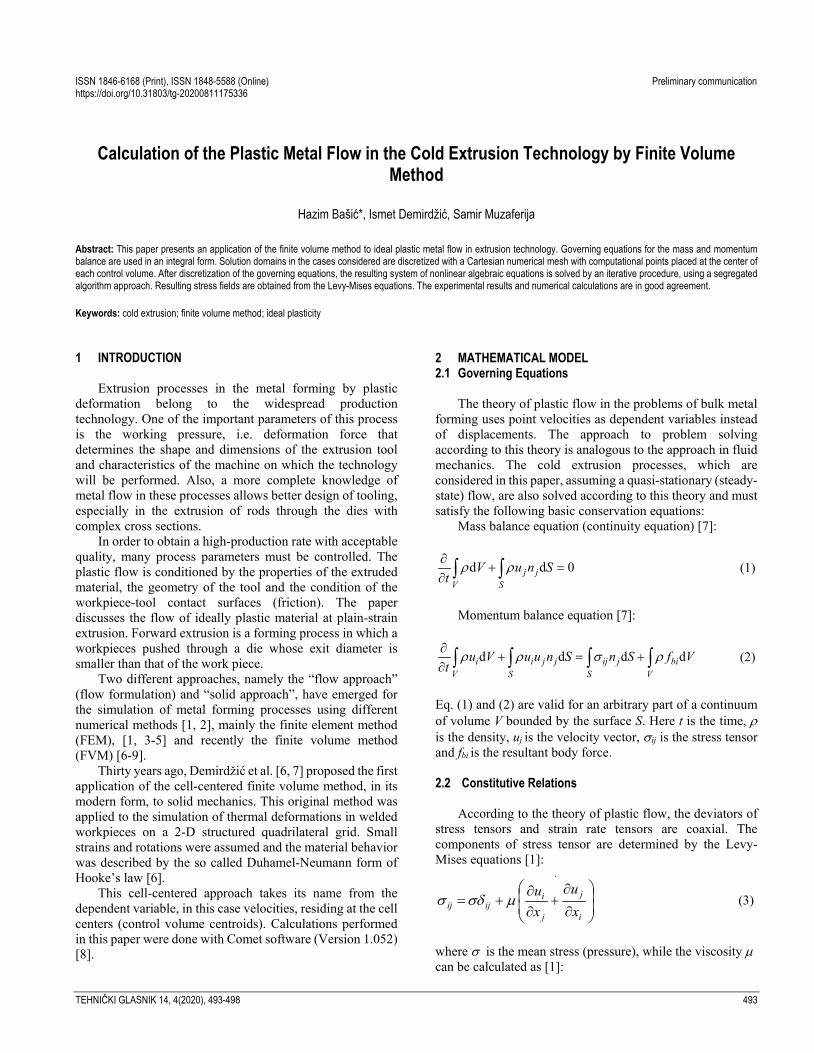
The two-dimensional spatial domain (the domain of solution) is sub-divided into a finite number (N) of contiguous control volumes (CV) or cells of volume V bounded by the surface S consisting of a number of cell faces of the area Sk. The solution domain is discretized by a rectangular numerical grid, example on Fig. 1.

Figure 1 Example of the 2D domain discretization

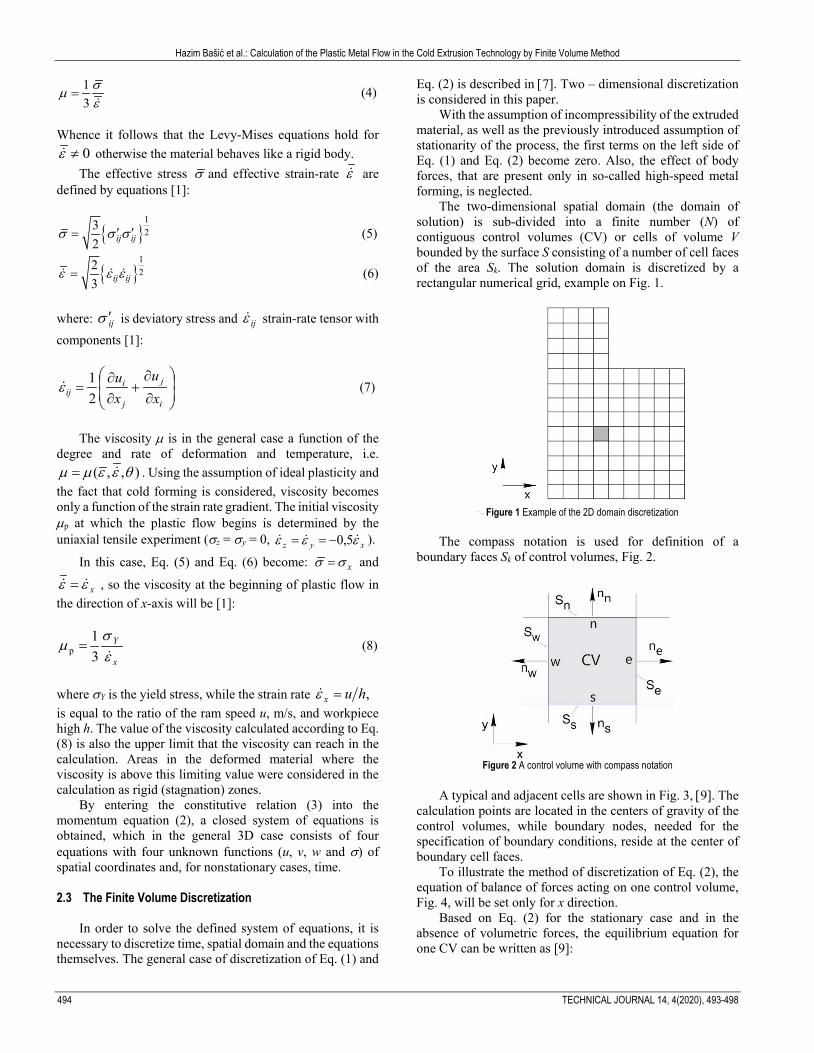
The compass notation is used for definition of a

boundary faces Sk of control volumes, Fig. 2.

Figure 2 A control volume with compass notation

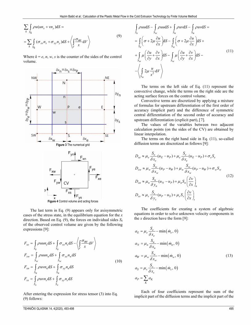
A typical and adjacent cells are shown in Fig. 3, [9]. The

calculation points are located in the centers of gravity of the control volumes, while boundary nodes, needed for the specification of boundary conditions, reside at the center of boundary cell faces.

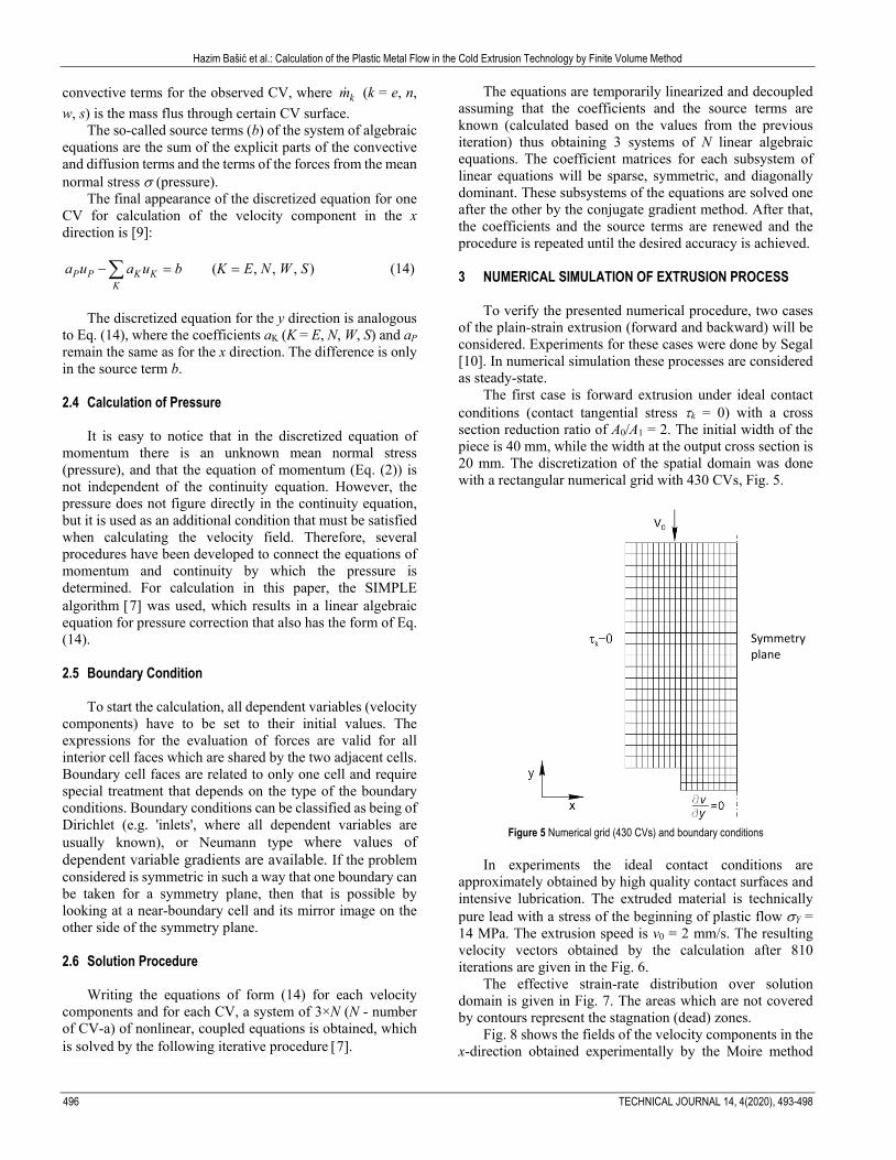
To illustrate the method of discretization of Eq. (2), the equation of balance of forces acting on one control volume, Fig. 4, will be set only for x direction.

Based on Eq. (2) for the stationary case and in the absence of volumetric forces, the equilibrium equation for one CV can be written as [9]:

Hazim Bašić et al.: Calculation of the Plastic Metal Flow in the Cold Extrusion Technology by Finite Volume Method

TEHNIČKI GLASNIK 14, 4(2020), 493-498 495

( )d

( )d d

x yk Sk

xx x xy yk S Vk

u un vn S

n n S Vxθθ

ρ

σσ σ

+ =

= + +

∑ ∫

∑ ∫ ∫ (9)

Where k = e, n, w, s is the counter of the sides of the control volume.

Figure 3 The numerical grid

Figure 4 Control volume and acting forces

The last term in Eq. (9) appears only for axisymmetric

cases of the stress state, in the equilibrium equation for the x direction. Based on Eq. (9), the forces on individual sides Sk of the observed control volume are given by the following expressions [9]:

d d d

d d

d d

d d

xe e xx eS S Ve e

xw w xx wS Sw w

xn n xy nS Sn n

xs s xy sS Ss s

F uun S n S Vx

F uun S n S

F uvn S n S

F uvn S n S

θθσρ σ

ρ σ

ρ σ

ρ σ

= + −

= +

= +

= +

∫ ∫ ∫

∫ ∫

∫ ∫

∫ ∫

(10)

After entering the expression for stress tensor (3) into Eq. (9) follows:

2

d d d d

2 d 2 d

d d

2 d

S S S Se w n n

S Se w

S Sw w

Sw

uu S uu S uv S uv S

u uS Sx x

u v u vS Sy x y x

u Vx

ρ ρ ρ ρ

σ µ σ µ

µ µ

µ

− + − =

∂ ∂ = + − + + ∂ ∂

∂ ∂ ∂ ∂+ + − + − ∂ ∂ ∂ ∂

−

∫ ∫ ∫ ∫

∫ ∫

∫ ∫

∫

(11)

The terms on the left side of Eq. (11) represent the

convective change, while the terms on the right side are the acting surface forces on the control volume.

Convective terms are discretized by applying a mixture of formulas for upstream differentiation of the first order of accuracy (implicit part) and the difference of symmetric central differentiation of the second order of accuracy and upstream differentiation (explicit part), [7].

The values of the variables between two adjacent calculation points (on the sides of the CV) are obtained by linear interpolation.

The terms on the right hand side in Eq. (11), so-called diffusion terms are discretized as follows [9]:

( ) ( )

( ) ( )

( )

( )

e exe e E P e E P e e

e e

w wxw w P W w P W w w

w w

nxn n N P n n

n n

sxs s P S s s

s s

S SD u u u u S

x xS S

D u u u u Sx x

S vD u u Sy x

S vD u u Sy x

µ µ σδ δ

µ µ σδ δ

µ µδ

µ µδ

≈ − + − +

≈ − + − +

∂ ≈ − + ∂ ∂ ≈ − + ∂

(12)

The coefficients for creating a system of algebraic

equations in order to solve unknown velocity components in the x direction have the form [9]:

( )

( )

( )

( )

min , 0

min , 0

min , 0

min , 0

eE e e

e

nN n n

n

wW w w

w

sS s s

s

P KK

Sa m

xS

a mxS

a mx

Sa m

xa a

µδ

µδ

µδ

µδ

= −

= −

= −

= −

= ∑

(13)

Each of four coefficients represent the sum of the

implicit part of the diffusion terms and the implicit part of the

Hazim Bašić et al.: Calculation of the Plastic Metal Flow in the Cold Extrusion Technology by Finite Volume Method

496 TECHNICAL JOURNAL 14, 4(2020), 493-498

convective terms for the observed CV, where km (k = e, n, w, s) is the mass flus through certain CV surface.

The so-called source terms (b) of the system of algebraic equations are the sum of the explicit parts of the convective and diffusion terms and the terms of the forces from the mean normal stress σ (pressure).

The final appearance of the discretized equation for one CV for calculation of the velocity component in the x direction is [9]:

( , , , )P P K KK

a u a u b K E N W S− = =∑ (14)

The discretized equation for the y direction is analogous

to Eq. (14), where the coefficients aK (K = E, N, W, S) and aP remain the same as for the x direction. The difference is only in the source term b.

2.4 Calculation of Pressure

It is easy to notice that in the discretized equation of momentum there is an unknown mean normal stress (pressure), and that the equation of momentum (Eq. (2)) is not independent of the continuity equation. However, the pressure does not figure directly in the continuity equation, but it is used as an additional condition that must be satisfied when calculating the velocity field. Therefore, several procedures have been developed to connect the equations of momentum and continuity by which the pressure is determined. For calculation in this paper, the SIMPLE algorithm [7] was used, which results in a linear algebraic equation for pressure correction that also has the form of Eq. (14). 2.5 Boundary Condition To start the calculation, all dependent variables (velocity components) have to be set to their initial values. The expressions for the evaluation of forces are valid for all interior cell faces which are shared by the two adjacent cells. Boundary cell faces are related to only one cell and require special treatment that depends on the type of the boundary conditions. Boundary conditions can be classified as being of Dirichlet (e.g. 'inlets', where all dependent variables are usually known), or Neumann type where values of dependent variable gradients are available. If the problem considered is symmetric in such a way that one boundary can be taken for a symmetry plane, then that is possible by looking at a near-boundary cell and its mirror image on the other side of the symmetry plane. 2.6 Solution Procedure Writing the equations of form (14) for each velocity components and for each CV, a system of 3×N (N - number of CV-a) of nonlinear, coupled equations is obtained, which is solved by the following iterative procedure [7].

The equations are temporarily linearized and decoupled assuming that the coefficients and the source terms are known (calculated based on the values from the previous iteration) thus obtaining 3 systems of N linear algebraic equations. The coefficient matrices for each subsystem of linear equations will be sparse, symmetric, and diagonally dominant. These subsystems of the equations are solved one after the other by the conjugate gradient method. After that, the coefficients and the source terms are renewed and the procedure is repeated until the desired accuracy is achieved. 3 NUMERICAL SIMULATION OF EXTRUSION PROCESS

To verify the presented numerical procedure, two cases of the plain-strain extrusion (forward and backward) will be considered. Experiments for these cases were done by Segal [10]. In numerical simulation these processes are considered as steady-state.

The first case is forward extrusion under ideal contact conditions (contact tangential stress τk = 0) with a cross section reduction ratio of A0/A1 = 2. The initial width of the piece is 40 mm, while the width at the output cross section is 20 mm. The discretization of the spatial domain was done with a rectangular numerical grid with 430 CVs, Fig. 5.

Figure 5 Numerical grid (430 CVs) and boundary conditions

In experiments the ideal contact conditions are

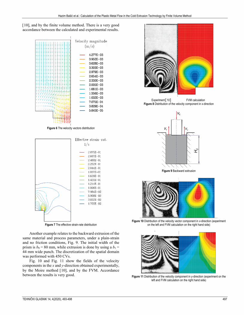
approximately obtained by high quality contact surfaces and intensive lubrication. The extruded material is technically pure lead with a stress of the beginning of plastic flow σY = 14 MPa. The extrusion speed is v0 = 2 mm/s. The resulting velocity vectors obtained by the calculation after 810 iterations are given in the Fig. 6.

The effective strain-rate distribution over solution domain is given in Fig. 7. The areas which are not covered by contours represent the stagnation (dead) zones.

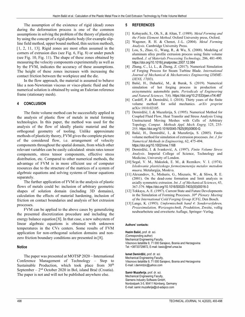
Fig. 8 shows the fields of the velocity components in the x-direction obtained experimentally by the Moire method

Symmetry plane

Hazim Bašić et al.: Calculation of the Plastic Metal Flow in the Cold Extrusion Technology by Finite Volume Method

TEHNIČKI GLASNIK 14, 4(2020), 493-498 497

[10], and by the finite volume method. There is a very good accordance between the calculated and experimental results.

Figure 6 The velocity vectors distribution

Figure 7 The effective strain-rate distribution

Another example relates to the backward extrusion of the

same material and process parameters, under a plain-strain and no friction conditions, Fig. 9. The initial width of the prism is b0 = 80 mm, while extrusion is done by using a b1 = 44 mm wide punch. The discretization of the spatial domain was performed with 450 CVs.

Fig. 10 and Fig. 11 show the fields of the velocity components in the x and y-direction obtained experimentally, by the Moire method [10], and by the FVM. Accordance between the results is very good.

Experiment [10] FVM calculation

Figure 8 Distribution of the velocity component in x-direction

Figure 9 Backward extrusion

Figure 10 Distribution of the velocity vector component in x-direction (experiment

on the left and FVM calculation on the right hand side)

Figure 11 Distribution of the velocity component in y-direction (experiment on the

left and FVM calculation on the right hand side)

Hazim Bašić et al.: Calculation of the Plastic Metal Flow in the Cold Extrusion Technology by Finite Volume Method

498 TECHNICAL JOURNAL 14, 4(2020), 493-498

The assumption of the existence of rigid (dead) zones during the deformation process is one of the common assumptions in solving the problem of the theory of plasticity by using the concept of a rigid-plastic body (for example slip-line field method, upper bound method, thin section method), [1, 2, 11, 13]. Rigid zones are most often assumed in the corners of extrusion dies (see Fig. 6, Fig. 8) or under punch (see Fig. 10, Fig. 11). The shape of these zones obtained by measuring the velocity components experimentally as well as by the FVM, indicates the accuracy of these assumptions. The height of these zones increases with increasing the contact friction between the workpiece and the die.

In the flow approach, the material is assumed to behave like a non-Newtonian viscous or visco-plastic fluid and the numerical solution is obtained by using an Eulerian reference frame (stationary mesh).

4 CONCLUSION

The finite volume method can be successfully applied in the analysis of plastic flow of metals in metal forming technologies. In this paper, the method was used for the analysis of the flow of ideally plastic material and the orthogonal geometry of tooling. Unlike approximate methods of plasticity theory, FVM gives the complete picture of the considered flow, i.e. arrangement of velocity components throughout the spatial domain, from which other relevant variables can be easily calculated: strain rates tensor components, stress tensor components, effective stress distribution, etc. Compared to other numerical methods, the advantage of FVM is in more efficient use of computer resources due to the structure of the matrices of a system of algebraic equations and solving systems of linear equations separately.

The further application of FVM in the analysis of plastic flows of metals could be: inclusion of arbitrary geometric shapes of solution domain (including 3D domains), calculation the effects of material hardening, inclusion of friction on contact boundaries and analysis of hot extrusion processes.

FVM can be applied to the above cases by generalizing the presented discretization procedure and including the energy balance equation [8]. In that case, a new subsystem of linear algebraic equations is obtained with unknown temperatures in the CVs centers. Some results of FVM application for non-orthogonal solution domains and non-zero friction boundary conditions are presented in [8].

Notice

The paper was presented at MOTSP 2020 – International Conference Management of Technology – Step to Sustainable Production, which took place from 30th September – 2nd October 2020 in Bol, island Brač (Croatia). The paper is not and will not be published anywhere else.

5 REFERENCES

[1] Kobayashi, S., Oh, S., & Altan, T. (1989). Metal Forming and the Finite Element Method. Oxford University press, Oxford.

[2] Wagoner, R. H. & Chenot, J.-L. (2004). Metal Forming Analysis. Cambridge University Press.

[3] Lou, S., Zhao, G., Wang, R., & Wu, X. (2008). Modeling of aluminum alloy profile extrusion process using finite volume method. J. of Materials Processing Technology, 206, 481-490. https://doi.org/10.1016/j.jmatprotec.2007.12.084

[4] Zhang, C., Li, L., & Zheng, Z. (2017). Numerical Simulation of Forging Process for Steam Turbine Blade. International Journal of Mechanical & Mechatronics Engineering IJMME-IJENS, 17(03).

[5] Bašić, H., Duharkić, M., & Burak, S. (2019). Numerical simulation of hot forging process in production of axisymmetric automobile parts. Periodicals of Engineering and Natural Sciences, 7(4). https://doi.org/10.21533/pen.v7i4.487

[6] Cardiff, P. & Demirdžić, I. (2018). Thirty years of the finite volume method for solid mechanics. arXiv preprint arXiv:1810.02105.

[7] Demirdžić, I. & Muzaferija, S. (1995). Numerical Method for Coupled Fluid Flow, Heat Transfer and Stress Analysis Using Unstructured Moving Meshes with Cells of Arbitrary Topology. Comput. Methods Appl. Mech. Engrg. 125, 235-255. https://doi.org/10.1016/0045-7825(95)00800-G

[8] Bašić, H., Demirdžić, I., & Muzaferija, S. (2005). Finite volume method for simulation of extrusion processes. Int. J. for Numerical Methods in Engineering, 62, 475-494. https://doi.org/10.1002/nme.1168

[9] Demirdžić, I. & Ivanković, A. (1997). Finite Volume Stress Analysis. Imperial College of Science, Technology and Medicine, University of London.

[10] Segal, V. M., Makušok, E. M., & Reznikov, V. I. (1974). Isledovanie plastičeskogo formoizmenenija metalov metodom muara, Metalurgija, Moskva.

[11] Alexandrov, S., Mishuris, G., Miszuris, W., & Sliwa, R. E. (2001). On the dead-zone formation and limit analysis in axially symmetric extrusion. Int. J. of Mechanical Sciences, 43, 367-379. https://doi.org/10.1016/S0020-7403(00)00016-3

[12] Tekkaya, A. E. (1997). Current State and Future Developments in the Simulation of Forming Processes. 30th Plenary Meeting of the International Cold Forging Group ICFG, Den Bosch.

[13] Lange, K. (1993). Umformtechnik band 4: Sonderverfahren, Prozesimulation, Werzeugtechnik, Produktion, Zweite, vollig neubearbeitete und erweiterte Auflage, Springer–Verlag.

Authors’ contacts:

Hazim Bašić, prof. dr. sci. (Corresponding author) Mechanical Engineering Faculty, Vilsonovo šetalište 9, 71 000 Sarajevo, Bosnia and Herzegovina Tel: +38733729872, E-mail: basic@mef.unsa.ba

Ismet Demirdžić, prof. dr. sci. Mechanical Engineering Faculty, Vilsonovo šetalište 9, 71 000 Sarajevo, Bosnia and Herzegovina E-mail: i.demirdzic@yahoo.com

Samir Muzaferija, prof. dr. sci. Mechanical Engineering Faculty, Siemens Industry Software GmbH, Nordostpark 3-5, 90411 Nürnberg, Germany E-mail: samir.muzaferija@cd-adapco.com