arXiv:hep-ph/0303146v1 18 Mar 2003 Calculation of fluxes of charged particles and neutrinos from atmospheric showers V.Plyaskin ∗ Institute of Theoretical and Experimental Physics, Moscow,Russia March 18, 2003. Abstract The results on the fluxes of charged particles and neutrinos from a 3-dimensional (3D) simulation of atmospheric showers are presented. An agreement of calculated fluxes with data on charged particles from the AMS and CAPRICE detectors is demonstrated. Predictions on neutrino fluxes at different experimental sites are compared with results from other calculations. 1 Introduction The interpretation of the data on atmospheric neutrinos from different experiments [1, 2, 3] relies on calculations of neutrino fluxes. The many calculations made in recent years [4, 5, 6, 7, 8, 9, 10, 11, 12] have been done using approaches invoking different models of the Earth’s magnetic field, different primary spectra of cosmic rays and methods of tracing them in the Earth’s magnetic field, as well as various models of production of secondaries in the inelastic interactions and the way the Earth’s magnetic field is influencing (or not) the propagation of these secondaries in the atmosphere. (For a review see [13]). In view of fundamental importance of results of calculations for the interpretations of the atmospheric neutrino anomaly, it is acknowledged that a comprehensive simulation of atmospheric showers is needed. However, because of big computing power required to perform this task, most calculations resort to some, presumably well argumented simpli- fications. In the previous work [10] 1 an attempt has been made to avoid these simplifica- tions. The calculations were based on the recent data from the AMS experiment [14] and * E-mail address: [email protected]1 A technical error in normalization of neutrino fluxes in Phys.Lett.B 516 is corrected for in hep-ph/0103286 v3. 1
Transcript
arX
iv:h
ep-p
h/03
0314
6v1
18
Mar
200
3
Calculation of fluxes of charged particlesand neutrinos from atmospheric showers
V.Plyaskin∗
Institute of Theoretical and Experimental Physics,
Moscow,Russia
March 18, 2003.
Abstract
The results on the fluxes of charged particles and neutrinos from a 3-dimensional(3D) simulation of atmospheric showers are presented. An agreement of calculatedfluxes with data on charged particles from the AMS and CAPRICE detectors isdemonstrated. Predictions on neutrino fluxes at different experimental sites arecompared with results from other calculations.
1 Introduction
The interpretation of the data on atmospheric neutrinos from different experiments [1, 2, 3]relies on calculations of neutrino fluxes. The many calculations made in recent years[4, 5, 6, 7, 8, 9, 10, 11, 12] have been done using approaches invoking different models ofthe Earth’s magnetic field, different primary spectra of cosmic rays and methods of tracingthem in the Earth’s magnetic field, as well as various models of production of secondariesin the inelastic interactions and the way the Earth’s magnetic field is influencing (or not)the propagation of these secondaries in the atmosphere. (For a review see [13]).
In view of fundamental importance of results of calculations for the interpretations ofthe atmospheric neutrino anomaly, it is acknowledged that a comprehensive simulationof atmospheric showers is needed. However, because of big computing power required toperform this task, most calculations resort to some, presumably well argumented simpli-fications. In the previous work [10]1 an attempt has been made to avoid these simplifica-tions. The calculations were based on the recent data from the AMS experiment [14] and
demonstrated a good agreement with experimental results in terms of fluxes of chargedsecondaries produced in atmospheric showers [14, 15].
The present study follows the same approach with some changes. Firstly, the rigidityrange of generated primary cosmic rays is extended from 100 to 500 GV. Secondly, thecontribution from helium nuclei is simulated directly in He interactions with atmosphereand not using the results from proton interactions. Finally, the statistics of this study isabout 3.5 times bigger and corresponds to ∼ 2.2 ps exposure.
2 Description of the model
The calculation is based on the GEANT3/GHEISHA package [16] adapted to the scaleof cosmic ray travel and interactions. The Earth is modeled to be a sphere of 6378.14 kmradius of a uniform density of 5.22 g/cm3. The atomic and nuclear properties of the Earthare taken to be those of Ge - the closest in density (5.32 g/cm3) element. The Earth’satmosphere is modeled by 1 km thick variable density layers of air extending up to 71 kmfrom the Earth’s surface. The density change with altitude is calculated using StandardAtmosphere Calculator [17]. The Earth’s magnetic field for the year 1998 is calculatedaccording to World Magnetic Field Model (WMM-2000) [18] with 6 degrees of sphericalharmonics.
The flux of primary protons and helium nuclei in the Solar system is parametrizedon the basis of the AMS data [14]. At the rigidities below several GV the spectrum iscorrected for the solar activity according to the 11 year solar cycle [19]. Isotropicallyemitted from a sphere of 10 Earth’s radii, the primary cosmic particles with kinematicparameters compatible with those reaching the Earth are traced in the magnetic fielduntil they interact with the atmosphere. The production of secondaries resulting frominteractions of He nuclei is treated using the superposition approximation [20]. Theleading primary and the secondary particles produced in the interactions are traced inthe magnetic field until they go below 0.125 GeV/c.
3 Comparison with experimental data
All results in this study are obtained directly without any renormalization. To comparethe calculated fluxes of charged particles with the AMS measurements [14] the overallfluxes produced in the simulation are restricted to the AMS acceptance during the zenithfacing flight period. Fig.1 shows the spectra of protons for different positions of AMSwith respect to the magnetic equator. As in the previous study the result of simulationcorrectly reproduces the spectra of both primary and secondary protons.
2
Protons in AMS
10-4
10-3
10-2
10-1
1
10-1
1 10 102
Flu
x (m
2 sr
s M
eV)-1
Kinetic Energy (GeV)
a)
10-4
10-3
10-2
10-1
1
10-1
1 10 102
Flu
x (m
2 sr
s M
eV)-1
Kinetic Energy (GeV)
b)
10-4
10-3
10-2
10-1
1
10-1
1 10 102
Flu
x (m
2 sr
s M
eV)-1
Kinetic Energy (GeV)
c)
10-4
10-3
10-2
10-1
1
10-1
1 10 102
Flu
x (m
2 sr
s M
eV)-1
Kinetic Energy (GeV)
d)
Figure 1: Proton flux in AMS at different magnetic latitudes (|ΘM |). Solid line - fluxfrom the top, dashed line - flux from the bottom. a) |ΘM | <0.2 rad, b) 0.2< |ΘM | <0.5rad, c) 0.5< |ΘM | <0.8 rad, c) 0.8< |ΘM | <1.1 rad. The dots are the AMS measurements[14].
3
Positron flux in AMS
10-4
10-3
10-2
10-1
1
10-1
1
Flu
x (m
2 sr
s M
eV)-1
Energy (GeV)
a)
10-4
10-3
10-2
10-1
1
10-1
1
Flu
x (m
2 sr
s M
eV)-1
Energy (GeV)
b)
10-4
10-3
10-2
10-1
1
10-1
1
Flu
x (m
2 sr
s M
eV)-1
Energy (GeV)
c)
10-4
10-3
10-2
10-1
1
10-1
1
Flu
x (m
2 sr
s M
eV)-1
Energy (GeV)
d)
Figure 2: Secondary positron flux in AMS at different magnetic latitudes (|ΘM |). Solidline - flux from the top, dashed line - flux from the bottom. a) |ΘM | <0.3 rad, b)0.3< |ΘM | <0.6 rad, c) 0.6< |ΘM | <0.8 rad, c) 0.8< |ΘM | <1.1 rad. The dots are theAMS measurements [14]. The enhancement at higher energies of the measured flux athigh magnetic latitude is due to primary cosmic positrons detected in the lower magneticcutoff region.
4
Electron flux in AMS
10-4
10-3
10-2
10-1
10-1
1
Flu
x (m
2 sr
s M
eV)-1
Energy (GeV)
a)
10-4
10-3
10-2
10-1
10-1
1
Flu
x (m
2 sr
s M
eV)-1
Energy (GeV)
b)
10-4
10-3
10-2
10-1
10-1
1
Flu
x (m
2 sr
s M
eV)-1
Energy (GeV)
c)
10-4
10-3
10-2
10-1
10-1
1
Flu
x (m
2 sr
s M
eV)-1
Energy (GeV)
d)
Figure 3: Secondary electron flux in AMS at different magnetic latitudes (|ΘM |). Solidline - flux from the top, dashed line - flux from the bottom. a) |ΘM | <0.3 rad, b)0.3< |ΘM | <0.6 rad, c) 0.6< |ΘM | <0.8 rad, d) 0.8< |ΘM | <1.1 rad. The dots are theAMS measurements [14]. The enhancement at higher energies of the measured flux athigh magnetic latitude is due to primary cosmic electrons detected in the lower magneticcutoff region.
5
Positron/electron flux ratio in AMS
0
0.5
1
1.5
2
2.5
3
3.5
4
4.5
5
0 0.1 0.2 0.3 0.4 0.5 0.6 0.7 0.8 0.9 1
e+/e
-
|ΘM|
Figure 4: Calculated dependence on magnetic latitude of positron/electron flux ratio.The dots are the AMS measurements [14].
6
Vertical muons at the sea level
10-1
1
10
10-1
1 10
dN/d
p µ(m
2 sr
s G
eV/c
)
pµ(GeV/c)
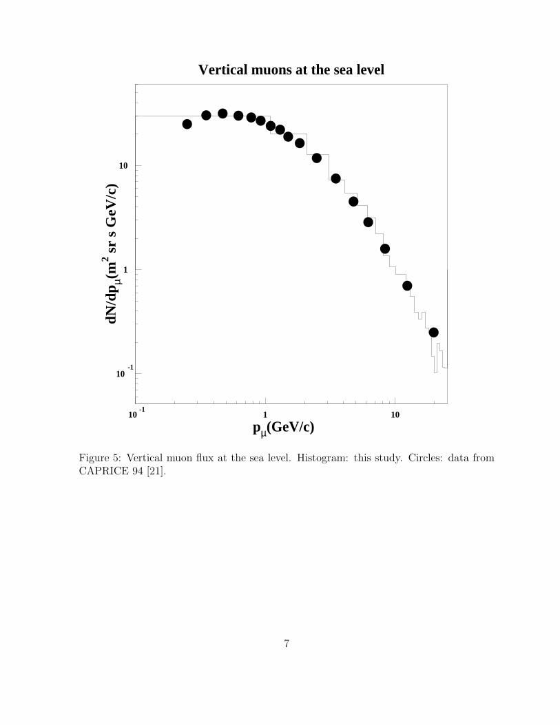
Figure 5: Vertical muon flux at the sea level. Histogram: this study. Circles: data fromCAPRICE 94 [21].
7
The simulated positron and electron spectra shown in Figs.2 and 3 are in good agree-ment with those obtained in the AMS experiment [14] allowing for still insufficient statis-tics of spiraling positrons and electrons in the equator region, where the spiraling sec-ondaries dominate. For detailed discussion of the behaviour of the secondaries see [10].The measured relative rate of secondary leptons and their dependence on the magneticlatitude is well reproduced by the simulation (Fig.4).
The histogram in Fig.5 shows the flux of cosmic muons within the acceptance of theCAPRICE 94 experiment. The calculated flux is in good agreement with the measuredone reported in [21].
A good agreement between the predictions of fluxes of charged secondaries provided bythis calculation and the measurements is a strong indication that the fluxes of neutrino,which are produced in the same decays as the charged particles (see Fig.16) are simulatedcorrectly.
4 Atmospheric neutrino fluxes
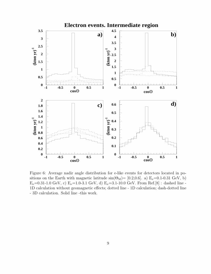
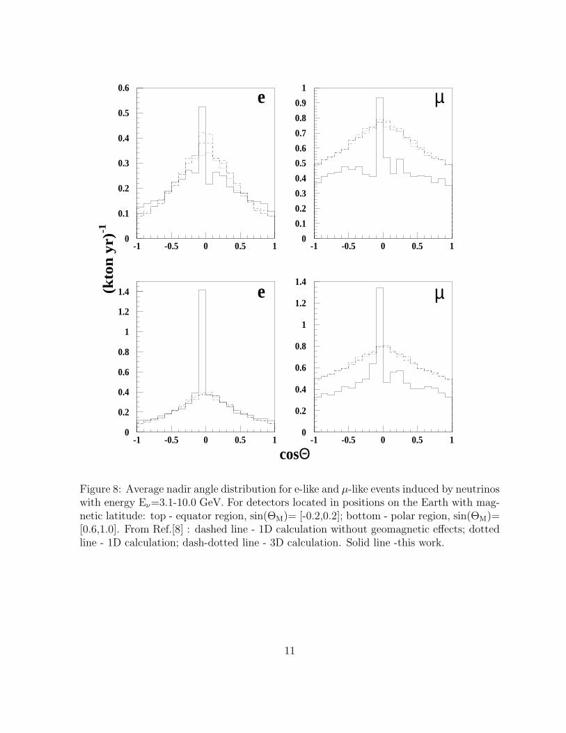
Figs.6,7,8 show the angular distributions of neutrino event rate in different regions ac-cording to the geomagnetic latitude calculated using the neutrino fluxes obtained in thiswork. These distributions are the result of convolution of neutrino fluxes with the neu-trino cross sections [22],[23],[24] and do not include detector related effects. The actualamount of detected neutrinos from those produced just under the Earth’s surface, which ismodeled as a simple sphere, depends on the actual detector position (depth underground,surrounding landscape). Compared to [8] the event rates from this work, given in Figs.6,7for the magnetic latitude region with sin(ΘM)= [0.2,0.6], are systematically higher forvery low, Eν=0.1-0.31 GeV, energy neutrinos, and are similar in the energy range ofEν=0.31-1.0 GeV. For higher energies of Eν=1.0-3.1 GeV this work predicts event rateswhich are at the level of 0.7-0.8 of the 3D calculation result of [8]. The important differ-ence with previous calculations is clearly visible in the highest neutrino energy range ofEν=3.1-10.0 GeV. On the one hand the angular distributions and the absolute event ratesfor e-like events are practically the same for all types of calculations. On the other handthe integral event rate for µ-like events is only about 0.6 of those predicted in [8] and theangular distribution of this events, apart form the angular region close to the horizontaldirection, is much flatter. This tendency is typical for high energy neutrino events at allmagnetic latitude regions (see Fig.8).
The neutrino flux at different experimental sites is calculated for the area ±12o in lati-tude and longitude with the center at (35o N, 142oE); (48o N, 98o W ) and (42o N, 13oE)and the depth underground of 520 (2700 mwe), 700 and 750 m for Kamioka, Soudan andGran Sasso sites correspondingly. Fig.9 shows the averaged over all directions differentialenergy spectra of different neutrinos and antineutrinos at the Kamioka site. The spectrafor Soudan and Gran Sasso sites are presented in Figs.10 and 11 correspondingly.
8
Electron events. Intermediate region
0
0.5
1
1.5
2
2.5
3
3.5
-1 -0.5 0 0.5 1
(kto
n yr
)-1
cosΘ
a)
0
0.5
1
1.5
2
2.5
3
3.5
4
4.5
-1 -0.5 0 0.5 1
(kto
n yr
)-1
cosΘ
b)
0
0.2
0.4
0.6
0.8
1
1.2
1.4
1.6
1.8
2
-1 -0.5 0 0.5 1
(kto
n yr
)-1
cosΘ
c)
0
0.1
0.2
0.3
0.4
0.5
0.6
-1 -0.5 0 0.5 1
(kto
n yr
)-1
cosΘ
d)
Figure 6: Average nadir angle distribution for e-like events for detectors located in po-sitions on the Earth with magnetic latitude sin(ΘM)= [0.2,0.6]. a) Eν=0.1-0.31 GeV, b)Eν=0.31-1.0 GeV, c) Eν=1.0-3.1 GeV, d) Eν=3.1-10.0 GeV. From Ref.[8] : dashed line -1D calculation without geomagnetic effects; dotted line - 1D calculation; dash-dotted line- 3D calculation. Solid line -this work.
9
Muon events. Intermediate region
0
1
2
3
4
5
6
7
-1 -0.5 0 0.5 1
(kto
n yr
)-1
cosΘ
a)
0
1
2
3
4
5
6
7
8
-1 -0.5 0 0.5 1
(kto
n yr
)-1
cosΘ
b)
0
0.5
1
1.5
2
2.5
3
-1 -0.5 0 0.5 1
(kto
n yr
)-1
cosΘ
c)
0
0.2
0.4
0.6
0.8
1
-1 -0.5 0 0.5 1
(kto
n yr
)-1
cosΘ
d)
Figure 7: Average nadir angle distribution for µ-like events for detectors located in po-sitions on the Earth with magnetic latitude sin(ΘM)= [0.2,0.6]. a) Eν=0.1-0.31 GeV, b)Eν=0.31-1.0 GeV, c) Eν=1.0-3.1 GeV, d) Eν=3.1-10.0 GeV. From Ref.[8] : dashed line -1D calculation without geomagnetic effects; dotted line - 1D calculation; dash-dotted line- 3D calculation. Solid line -this work.
10
0
0.1
0.2
0.3
0.4
0.5
0.6
-1 -0.5 0 0.5 1
(kto
n y
r)-1
e
0
0.1
0.2
0.3
0.4
0.5
0.6
0.7
0.8
0.9
1
-1 -0.5 0 0.5 1
µ
0
0.2
0.4
0.6
0.8
1
1.2
1.4
-1 -0.5 0 0.5 1
e
0
0.2
0.4
0.6
0.8
1
1.2
1.4
-1 -0.5 0 0.5 1
cosΘ
µ
Figure 8: Average nadir angle distribution for e-like and µ-like events induced by neutrinoswith energy Eν=3.1-10.0 GeV. For detectors located in positions on the Earth with mag-netic latitude: top - equator region, sin(ΘM)= [-0.2,0.2]; bottom - polar region, sin(ΘM)=[0.6,1.0]. From Ref.[8] : dashed line - 1D calculation without geomagnetic effects; dottedline - 1D calculation; dash-dotted line - 3D calculation. Solid line -this work.
11
Neutrinos at the Kamioka site
1
10
10 2
10 3
10 4
10-2
10-1
1
Flu
x (m
2 sr
s G
eV)-1
Energy (GeV)
a)
1
10
10 2
10 3
10 4
10-2
10-1
1
Flu
x (m
2 sr
s G
eV)-1
Energy (GeV)
b)
1
10
10 2
10 3
10 4
10-2
10-1
1
Flu
x (m
2 sr
s G
eV)-1
Energy (GeV)
c)
1
10
10 2
10 3
10 4
10-2
10-1
1
Flu
x (m
2 sr
s G
eV)-1
Energy (GeV)
d)
Figure 9: Differential energy spectra of atmospheric neutrino (averaged over all directions)at the Kamioka site. a) νe, b) ν̄e, c) νµ, d) ν̄µ. Asterisks from Ref. [7], open circles fromRef. [5], triangles from Ref. [6], stars from Ref.[9]. Histograms - this work.
12
Neutrinos at the Soudan site
10
10 2
10 3
10 4
10-2
10-1
1
Flu
x (m
2 sr
s G
eV)-1
Energy (GeV)
a)
10
10 2
10 3
10 4
10-2
10-1
1
Flu
x (m
2 sr
s G
eV)-1
Energy (GeV)
b)
10
10 2
10 3
10 4
10-2
10-1
1
Flu
x (m
2 sr
s G
eV)-1
Energy (GeV)
c)
10
10 2
10 3
10 4
10-2
10-1
1
Flu
x (m
2 sr
s G
eV)-1
Energy (GeV)
d)
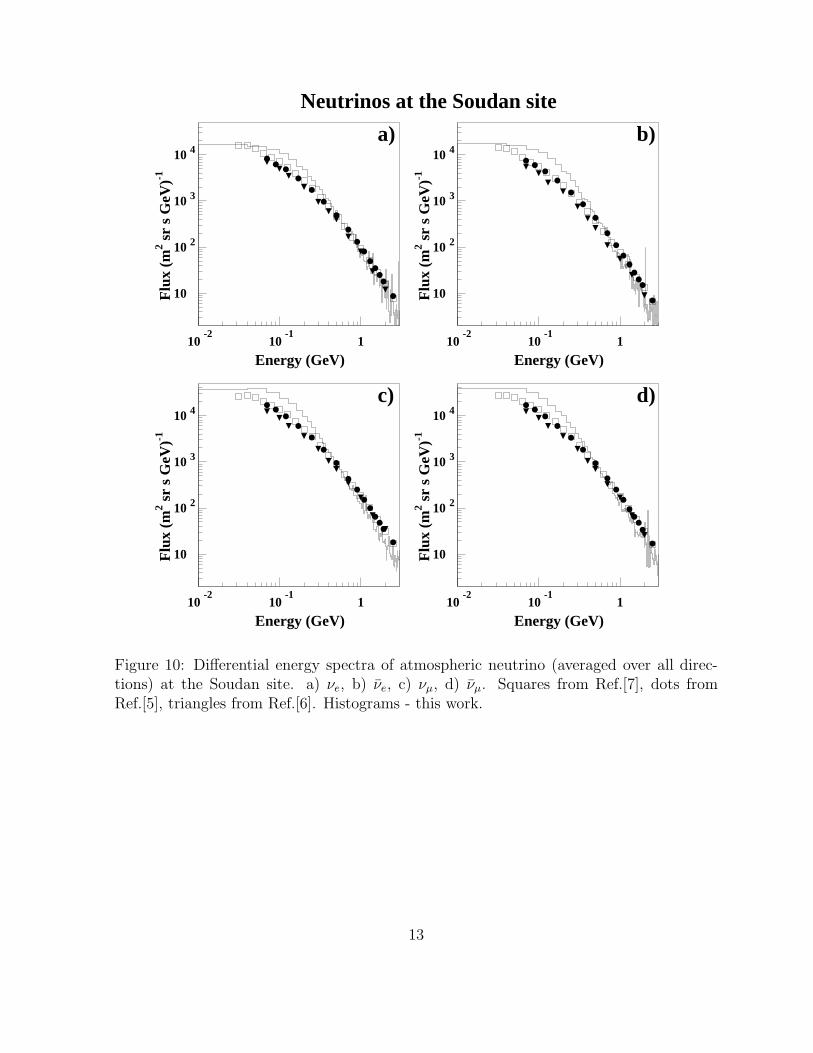
Figure 10: Differential energy spectra of atmospheric neutrino (averaged over all direc-tions) at the Soudan site. a) νe, b) ν̄e, c) νµ, d) ν̄µ. Squares from Ref.[7], dots fromRef.[5], triangles from Ref.[6]. Histograms - this work.
13
Neutrinos at the Gran Sasso site
1
10
10 2
10 3
10 4
10-2
10-1
1
Flu
x (m
2 sr
s G
eV)-1
Energy (GeV)
a)
1
10
10 2
10 3
10 4
10-2
10-1
1
Flu
x (m
2 sr
s G
eV)-1
Energy (GeV)
b)
1
10
10 2
10 3
10 4
10-2
10-1
1
Flu
x (m
2 sr
s G
eV)-1
Energy (GeV)
c)
1
10
10 2
10 3
10 4
10-2
10-1
1
Flu
x (m
2 sr
s G
eV)-1
Energy (GeV)
d)
Figure 11: Differential energy spectra of atmospheric neutrino (averaged over all direc-tions) at the Gran Sasso site. a) νe, b) ν̄e c) νµ, d) ν̄µ. Dots from Ref.[5]. Histograms -this work.
14
0
0.5
1
1.5
2
2.5
3
3.5
4
4.5
5
0 1 2 3
Flu
x (
KH
z m
-2 s
r-1
)
φ(rad)
0
1
2
3
4
5
6
7
0 1 2 30
2
4
6
8
10
0 1 2 3
0.4
0.5
0.6
0.7
0.8
0.9
1
1.1
1.2
-2 -1 0
Do
wn
/up
flu
x r
ati
o
log10
E(GeV)
0.6
0.8
1
1.2
1.4
1.6
1.8
2
-2 -1 00.5
0.6
0.7
0.8
0.9
1
1.1
1.2
1.3
-2 -1 0
1.6
1.8
2
2.2
2.4
2.6
2.8
-1 -0.5 0 0.5 1
νµ/ν
e f
lux
ra
tio
cosΘ
1.6
1.8
2
2.2
2.4
2.6
2.8
-1 -0.5 0 0.5 1
1.6
1.8
2
2.2
2.4
2.6
2.8
-1 -0.5 0 0.5 1
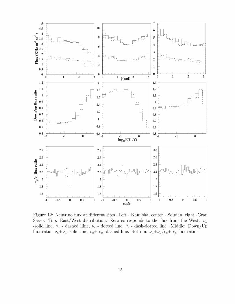
Figure 12: Neutrino flux at different sites. Left - Kamioka, center - Soudan, right -GranSasso. Top: East/West distribution. Zero corresponds to the flux from the West. νµ-solid line, ν̄µ - dashed lilne, νe - dotted line, ν̄e - dash-dotted line. Middle: Down/Upflux ratio. νµ+ν̄µ -solid line, νe+ ν̄e -dashed line. Bottom: νµ+ν̄µ/νe+ ν̄e flux ratio.
15
10-2
10-1
1
-1 -0.5 0 0.5 1
10-1
1
-1 -0.5 0 0.5 1
10-2
10-1
1
10
-1 -0.5 0 0.5 1
Flu
x (K
Hz
m-2
sr-1
)
10-1
1
10
-1 -0.5 0 0.5 1
10-2
10-1
1
10
-1 -0.5 0 0.5 1
10-1
1
10
-1 -0.5 0 0.5 1
cosΘ
Figure 13: Angular dependence of neutrino flux at different sites. Top - Kamioka, middle- Soudan, bottom - Gran Sasso. Left column - νe+ ν̄e, right column - νµ+ν̄µ. Neutrinoenergy: Dotted line - 0.1< Eν <0.31 GeV; dashed line - 0.31< Eν <1.0 GeV; solid line -Eν >1.0 GeV.
16
ν µ/ν e f
lux
rati
o
cosΘ
Figure 14: Angular dependence of νµ+ν̄µ / νe+ν̄e flux ratio at different sites. Neutrinoenergy: left column 0.1< Eν <0.31 GeV; central column 0.31< Eν <1.0 GeV; rightcolumn Eν >1.0 GeV. Top raw - Kamioka site; middle raw - Soudan site; bottom raw -Gran Sasso site. The error bars give statistical errors.
17
In comparison with predictions of previous calculations made for this sites [5, 6, 7, 9]there is an excess of low energy and a deficit of high energy neutrinos. The same tendencyis reported in [11]. The extent of these differences depends on the given site and is notthe same for different kinds of neutrino.
From Fig.12 one can see that there is a considerable difference both in East/Westand down/up asymmetry of the fluxes at different sites. At the same time the ratio ofmuon(νµ + ν̄µ) to electron(νe + ν̄e) neutrino fluxes, dominated by low energy neutrinos,appears to be constant at all sites and independent on the direction of neutrinos withrespect to the surface of the Earth. The situation is much different if one considersdifferent neutrino energy intervals (Fig.13). As it is shown in Fig.14 the muon/electronneutrino flux ratio is constant only for low energy neutrinos. With the increase of neutrinoenergy the ratio behaves differently at different sites, although there is a clear tendencytowards smaller values of muon/electron neutrino flux ratio for directions approachinghorizontal. This effect, reported in our previous work [10] is confirmed by the presenthigher statistics calculations.
5 Discussion
The neutrino fluxes predicted in this work for different locations have the energy spectra,relative intensity and angular distributions different from those obtained by other authors.There are several points in calculations which can explain these differences.
5.1 Primary cosmic ray flux
It is recognized, that the primary cosmic ray spectrum is a major source of uncertaintyin calculations of atmospheric neutrino fluxes. As it was demonstrated in section 3, theprimary proton flux calculated using the forward tracing method fits well the AMS data.In this section we present the results on primary proton flux at different magnetic latitudesobtained using the backward tracing method commonly used as a standard procedure inatmospheric neutrino flux calculations. In this study the protons with the interstellarrigidity spectra are isotropically emitted from a sphere situated at the the top of theatmosphere at 70 km from the Earth’s surface and are traced following the backwardpath of a particle with the same rigidity but of the opposite charge. Only particles back-traced to a large distance (10 Earth’s radii) are considered as following an ”allowed”trajectory.
The flux of primary protons with ”allowed” trajectories passing through a detectionplane from the top hemisphere is shown in Fig.15 for different magnetic latitude regions.The detection sphere is assumed to be at 400 km, corresponding to the AMS flight altitude.
18
0.001
0.002
0.003
0.004
0.005
0.006
0.007
10-1
1 10 102
Flu
x (m
2 sr
s M
eV)-1
Kinetic Energy (GeV)
a)
0.001
0.002
0.003
0.004
0.005
0.006
0.007
0.008
0.009
0.01
10-1
1 10 102
Flu
x (m
2 sr
s M
eV)-1
Kinetic Energy (GeV)
b)
0.01
0.02
0.03
0.04
0.05
0.06
0.07
0.08
10-1
1 10 102
Flu
x (m
2 sr
s M
eV)-1
Kinetic Energy (GeV)
c)
0.1
0.2
0.3
0.4
0.5
0.6
0.7
0.8
10-1
1 10 102
Flu
x (m
2 sr
s M
eV)-1
Kinetic Energy (GeV)
d)
Figure 15: Proton flux in AMS at different magnetic latitudes (|ΘM |). Solid line - backtracing, dashed line - forward tracing. a) |ΘM | <0.2 rad, b) 0.2< |ΘM | <0.5 rad, c)0.5< |ΘM | <0.8 rad, c) 0.8< |ΘM | <1.1 rad. The dots are the AMS measurements [14].
19
A comparison with AMS measurements (see Fig.15) shows that the cutoff value atdifferent magnetic latitudes is predicted correctly for both backward and forward tracing.However, at variance with predictions obtained with forward tracing, the flux of ”allowed”backtraced protons approaches the measured values only above 40 GeV and is far belowelsewhere [25]. For protons responsible for production of low energy neutrinos it is about 2times less then in the experiment. This deficit in primary flux intensity could be a reasonfor the lower fluxes and, consequently event rates, predicted for low energy neutrinos inprevious calculations as compared with the present one.
e- e+
e-
π-
µ-
µ-
νe
π-π+
π+
µ+
µ+
PP
Atmosphere
West East
νe
νe
–
–
–
–
–
–
νµ νµ
νµ
νµνµ
νµ
e+
νe
νµ νµ
Earth
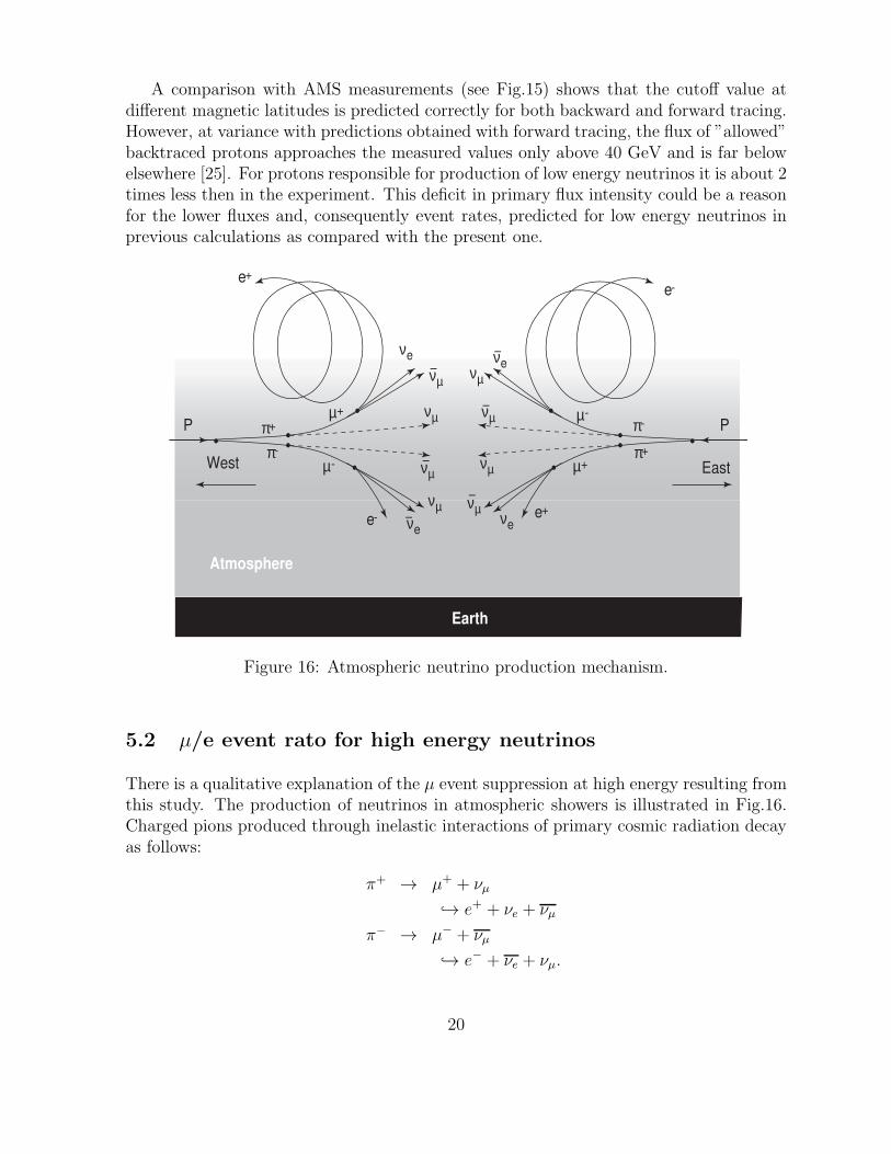
Figure 16: Atmospheric neutrino production mechanism.
5.2 µ/e event rato for high energy neutrinos
There is a qualitative explanation of the µ event suppression at high energy resulting fromthis study. The production of neutrinos in atmospheric showers is illustrated in Fig.16.Charged pions produced through inelastic interactions of primary cosmic radiation decayas follows:
π+ → µ+ + νµ
→֒ e+ + νe + νµ
π− → µ− + νµ
→֒ e− + νe + νµ.
20
Due to the Earth’s magnetic field a charged particle is deflected before decay from itsinitial direction. The deflection, ∆Θ, is practically independent of the particle momentum,p,
∆Θ =L
R∼ γ
p=
√p2 +m2
mp≃ const
m,
where L is the decay path length and R is the radius of curvature of the particle track inthe magnetic field.
For pions the mean decay length is short (cτπ=7.8 m) and, consequently, the meandeflection is very small (∆Θπ ≃ 0.4 mrad). For muons the mean decay length is about100 times longer (cτµ=658.6 m) resulting in a mean muon deflection before decay, ∆Θµ ≃3o. Albeit relatively small, this deflection is sufficient to direct most of neutrinos fromatmospheric muon decays towards the ground, even allowing for the Earth’s sphericalshape.
Thus, the neutrinos from π+ → µ+νµ and π− → µ−ν̄µ decays of pions producedin the atmosphere and going nearly parallel to horizon never reach the surface of theEarth. On the other hand (a half of) neutrinos from muon decays are emitted towardsthe Earth. Assuming equal flux from the East and the West, which is the case for highenergy neutrinos produced by high energy cosmic rays, one gets for the nearly horizontalflux: νµ and ν̄e from the West and ν̄µ and νe from the East (see Fig.16), and for the muonto electron event ratio:
µ
e=
νµ + ν̄µ
ν̄e + νe= 1.
All neutrinos from the vertical direction reach the Earth’s surface. This gives for theevent ratio:
µ
e=
(νµ + ν̄µ) + (ν̄µ + νµ)
ν̄e + νe= 2
in agreement with results of the present calculations.
5.3 Hadronic interaction models
Different groups use different models to simulate production of secondaries in the atmo-spheric showers. Independent of the method used, all models are eventually fine tunedusing as much available experimental data as possible. The GHEISHA code of simulationof hadronic interactions used in this study is not an exception.
There is a certain amount of criticism of GHEISHA in connection with neutrino fluxcalculations [11, 12, 26] based on direct model tests presented in [27, 28].
The inability of GHEISHA to predict the properties of residual nuclear fragmentsand the related problems with momentum/energy conservation may be of importance
21
in calorimetry, but have no pertinence to the secondaries responsible for production ofcharged leptons and neutrinos in the energy range considered in this study.
The results of [27] are relevant for proton interactions with relatively heavy (A>27)nuclei at proton energies Elab <1 GeV i.e. the region of energies too low to affect atmo-spheric neutrino fluxes.
In [28] the interactions of pions with several nuclei are studied. It is acknowledgedthat as far as secondary pion multiplicity and Feynman x distributions are concernedGHEISHA behaves well up to the pion energies as high as 100 GeV. At the same timethere are some deviations from experimental data, especially for heavy nuclei, in transversemomenta and rapidity distributions of the secondaries. These deviations can not seriouslyinfluence the results of atmospheric shower simulations.
An atmospheric shower is developing in the medium of rapidly changing density. Aparticle arriving vertically with respect to the Earth’s surface pass through an equiva-lent of one nuclear interaction length when it reaches an altitude of about 17 km. Theequivalent of second interaction length is attained at about 13 km. At these altitudes thedensity of atmosphere is 1/10 and 1/5 of air density at the ground level respectively. Thiscorresponds to nuclear interaction length of about 13 km and 3.5 km respectively. A pionof energy as high as 20 GeV has a mean decay length of only about 1 km. Consequently,charged pions produced in atmospheric showers mostly decay in flight and do not interactwith atmosphere. For the neutrino fluxes, it means that the effect of inaccuracy in angulardistributions of secondary pions reported in [28] is washed out by the change in directionof pions in the Earth’s magnetic field and the subsequent pion decay.
6 Conclusions
Our calculations are based on the up-to-date data on the cosmic ray fluxes measured by theAMS detector [14]. The atmospheric showers are simulated with as little simplificationsas possible at all stages of primary and secondary particle travel and interaction with theatmosphere. The difference in angular distributions of the ratios of fluxes of different kindsof neutrino at different sites and their dependence on the neutrino energy reported in [10]is confirmed on the basis of higher statistics. The angular distributions and the neutrinoevent rates obtained in this study suggest a possibility to describe the experimental resultson the high energy atmospheric neutrino fluxes [2, 3] without evoking muon neutrinooscillations.
The good agreement between charged secondary particle spectra produced in this cal-culation and experimental data from AMS [14] and CAPRICE [21] supports the viabilityof the result on atmospheric neutrino fluxes.
Acknowlegements. I’m grateful to Prof.Yu.Galaktionov for very useful and stimu-lating discussions.
22
References
[1] IMB collaboration, D.Casper et al, Phys. Rev. Lett. 66, 2561 (1991); R.Becker-Szendyet al, Phys. Rev. D 46, 3720 (1992);
Kamiokande collaboration, K.S.Hirata et al, Phys. Lett. B 205, 416 (1988); Phys.Lett. B 289, 146 (1992);
Y.Fukuda et al, Phys. Lett. B 335, 237 (1994);
Super-Kamiokande collaboration, Y.Fukuda et al, Phys. Rev. Lett. 81, 1562 (1998);
Super-Kamiokande collaboration, T.Futagami et al, Phys. Rev. Lett. 82, 5194 (1999);
Soudan collaboration, W.W.M.Allison et al, Phys. Lett. B 434, 137 (1999).
[2] Super-Kamiokande collaboration,S. Hatakeyama, et al, Phys.Rev.Lett. 81 2016(1998)
[3] MACRO collaboration, Phys. Lett. B 434, 451 (1998); Phys.Lett.B 478, 5 (2000).
[4] L.V.Volkova, Yad.Fiz. 31, 1510 (1980) also in Sov.J.Nucl.Phys. 31, 784 (1980);
A.V.Butkevich, L.G.Dedenko and I.M.Zheleznykh, Yad.Fiz. 50, 142 (1989) also inSov.J.Nucl.Phys. 50, 90 (1989);
G.Barr,T.K.Gaisser and T.Stanev,Phys. Rev. D 38, 85 (1989);
M.Honda et al, Phys. Lett. B 248, 193 (1990);
P.Lipari, Astroparticle Physics 1, 195 (1993);
V.Agraval et al, Phys. Rev. D 53, 1314 (1996);
P.Lipari,T.K.Gaisser and T.Stanev, Phys. Rev. D 58, 3003 (1998).
P.Lipari, hep-ph/0003013 (2000);
G.Battistoni et al, Astroparticle Physics 12, 315 (2000);
M.Honda et al, Phys.Rev.D 64 053011 (2001)
V.Naumov, hep-ph/0201310 v1 (2002);
Y.Liu et al. astro-ph/00211632 v1 (2002).
J.Tserkovnyak et al ,Astropart.Phys.18, 449 (2003).
[5] G.Barr,T.K.Gaisser and T.Stanev, Phys. Rev. D 39, 3532 (1989).
[6] E.V.Bugaev and V.A.Naumov, Phys. Lett. B 232, 391 (1989).
[7] M.Honda et al, Phys. Rev. D 52, 4985 (1995).
[8] P.Lipari, Astropart. Phys. 14, 153 (2000).
[9] G.Fiorentini et al, Phys. Lett. B 510, 173 (2001) .
23
[10] V.Plyaskin, Phys.Lett. B 516, 213 (2001) and hep-ph/0103286 v3 (2002).
[11] G.Battistoni et al. hep-ph/0307035 v1 (2002).
[14] AMS collaboration, Phys. Lett. B 472, 215 (2000);
AMS collaboration, Phys. Lett. B 484, 10 (2000);
AMS collaboration, Phys.Rep. 366, 331 (2002).
[15] O.C.Allkofer et al. Phys. Lett. B36, 425 (1971); B.C.Rastin,J.Phys. G10, 1609 (1984).
[16] GEANT 3, CERN DD/EE/84-1, Revised, 1987
[17] US Standard Atmosphere. see e.g. S.E.Forsythe, Smithsonian phusical ta-bles.(Smithsonian Institution press.Washington,DC, 1969)
[18] S.MacMillan et al, Journal of Geomagnetism and Geoelectricity, 49, 229 (1997);J.M.Quinn et al, Journal of Geomagnetism and Geoelectricity, 49, 245 (1997);


![arXiv:1208.1171v1 [astro-ph.EP] 6 Aug 20122 Cosmic rays at the sea level Muons are the dominant component of charged particles at sea level. The integral fluxes of particles arriving](https://static.documents.pub/doc/80x56/607a54bbaa44ac22705cb6df/arxiv12081171v1-astro-phep-6-aug-2012-2-cosmic-rays-at-the-sea-level-muons.jpg)


