33
28-Oct-11 1 Lecture 14 Power Engineering - Egill Benedikt Hreinsson Calculations of Capacitance for Transposed Bundled Conductor Transmission Lines
28-Oct-11
1Lecture 14 Power Engineering - Egill Benedikt Hreinsson
Calculations of Capacitance for Transposed Bundled Conductor
Transmission Lines
28-Oct-11
2Lecture 14 Power Engineering - Egill Benedikt Hreinsson
Multi-conductor Lines. An example with a 2 conductor bundle
h1
h1
+q1/2 +q1/2D13
D23
D'23
D'13
D'12
D12h2
h2
h3
h3
+q2/2 +q2/2
+q3/2 +q3/2
-q1/2 -q1/2
-q2/2 -q2/2
-q3/2 -q3/2
1 1 2,1,
12
1 1 1 1ln ln ln2 2 2 2a I
q q qVr d Dπε
⎧ ⎫= + + +⎨ ⎬
⎩ ⎭
1 1,2,
1 1 1ln ln2 2 2a I
q qVr dπε
⎧ ⎫= + +⎨ ⎬⎩ ⎭
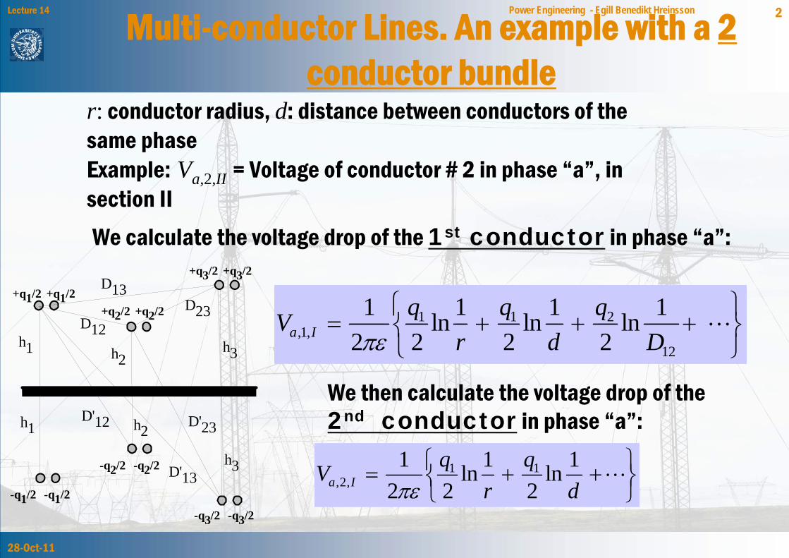
r: conductor radius, d: distance between conductors of the same phaseExample: Va,2,II = Voltage of conductor # 2 in phase “a”, in section IIWe calculate the voltage drop of the 1st conductor in phase “a”:
We then calculate the voltage drop of the 2nd conductor in phase “a”:
28-Oct-11
3Lecture 14 Power Engineering - Egill Benedikt Hreinsson
Multi-conductor Lines (2)
h1
h1
+q1/2 +q1/2D13
D23
D'23
D'13
D'12
D12h2
h2
h3
h3
+q2/2 +q2/2
+q3/2 +q3/2
-q1/2 -q1/2
-q2/2 -q2/2
-q3/2 -q3/2
,1, ,2,, 2
a II a IIa II
V VV
+=
,1, ,2,, 2
a III a IIIa III
V VV
+=
,1, ,2,, 2
a I a Ia I
V VV
+=
, , ,
3a I a II a III
a
V V VV
+ +=
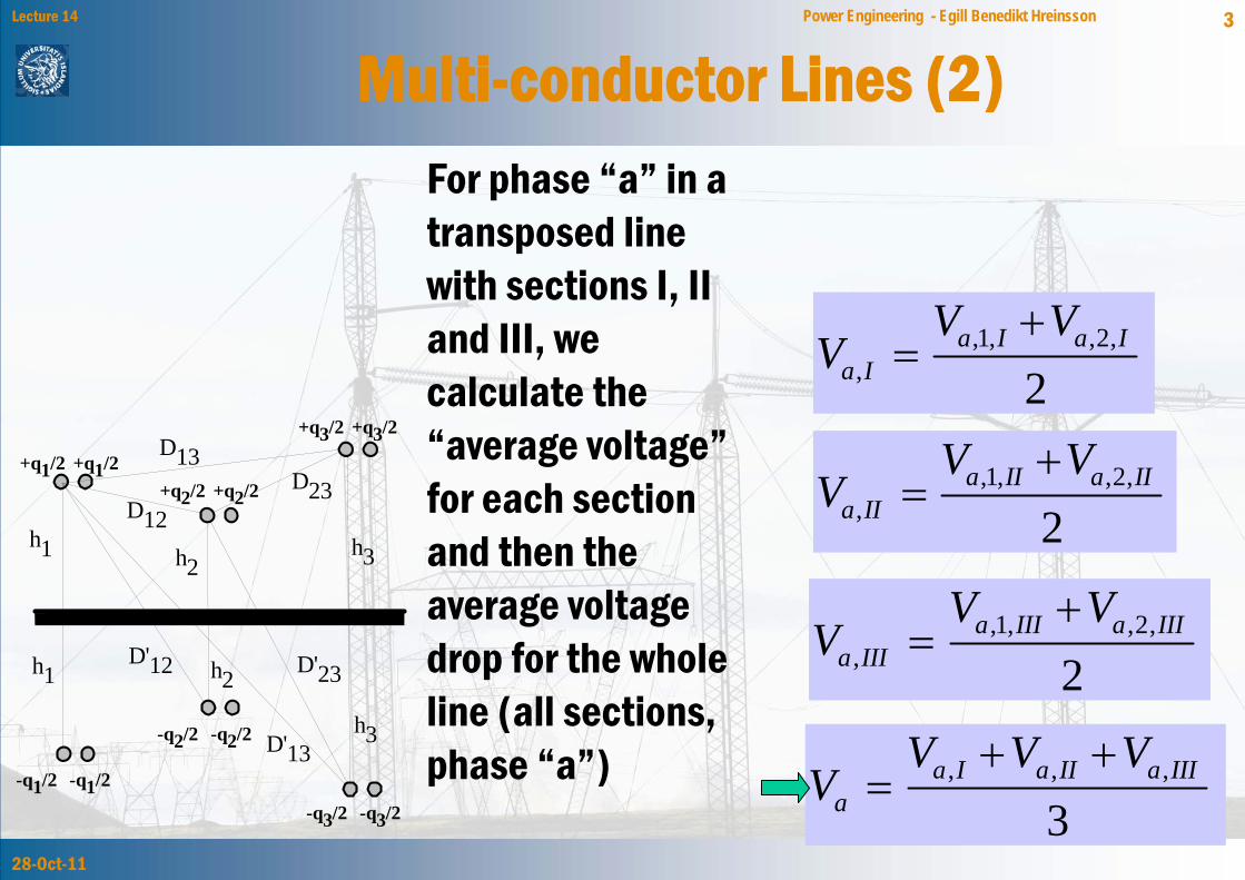
For phase “a” in a transposed line with sections I, II and III, we calculate the “average voltage”for each section and then the average voltage drop for the whole line (all sections, phase “a”)

28-Oct-11
4Lecture 14 Power Engineering - Egill Benedikt HreinssonGeometric Mean of Heights - Bundled Conductors
ha hb
DaDb
+qi/2 +qi/2
-qi/2 -qi/2
Phase # "i"
Image of phase # "i"
422
babai
DDhhh ⋅⋅⋅=
We get a combination of factor with logarithms that for instance lead to roots as follows

28-Oct-11
5Lecture 14 Power Engineering - Egill Benedikt Hreinsson
Geometric Mean Distances to Images
Da
D'a
Db
D'b
Dc
D'c
Dd
D'd
+qi/2+qi/2
-qj/2 -qj/2
phase # "i"
Image of phase # "j"
+qj/2 +qj/2
phase # "j"
4dcbaij DDDDD ⋅⋅⋅=
4dcbaij DDDDD ′⋅′⋅′⋅′=′
Similarly for a combination of distances between phases These lead to roots as follows:

28-Oct-11
6Lecture 14 Power Engineering - Egill Benedikt Hreinsson
Effective Radius - Bundled Conductors
24 32R r d d d R r d R r d= ⋅ ⋅ ⋅ = ⋅ = ⋅
d
d
-qj/4-qj/4
A phase with 4 conductors
A phase with 3 conductors
A phase with 2 conductors
-qj/4-qj/4 d
dd
-qj/3
-qj/3
-qj/3d
-qj/2 -qj/2 -qj
R r=
Radius of each conductor = rThe effective radius of each
conductor bundle = R. Compare with the GMR
A phase with 1 conductor

28-Oct-11
7Lecture 14 Power Engineering - Egill Benedikt Hreinsson
Summary of capacitance calculations
22ln
'
rCh D
R D
πε=
⎛ ⎞⋅⎜ ⎟⎝ ⎠
312 23 31D D D D= 3
12 23 31' ' ' 'D D D D=
31 2 3h h h h=
24 32R r d d d R r d R r d= ⋅ ⋅ ⋅ = ⋅ = ⋅
2
lnrC
DR
πε=With earth’s
influence:Without earth’s influence:

28-Oct-11
8Lecture 14 Power Engineering - Egill Benedikt Hreinsson
Capacitance - Inductance Relation
28-Oct-11
9Lecture 14 Power Engineering - Egill Benedikt Hreinsson
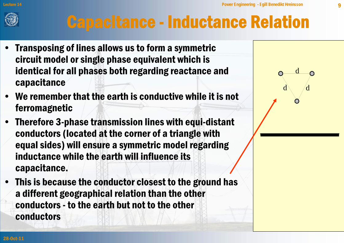
Capacitance - Inductance Relation• Transposing of lines allows us to form a symmetric
circuit model or single phase equivalent which is identical for all phases both regarding reactance and capacitance
• We remember that the earth is conductive while it is not ferromagnetic
• Therefore 3-phase transmission lines with equi-distant conductors (located at the corner of a triangle with equal sides) will ensure a symmetric model regarding inductance while the earth will influence its capacitance.
• This is because the conductor closest to the ground has a different geographical relation than the other conductors - to the earth but not to the other conductors
d
dd
28-Oct-11
10Lecture 14 Power Engineering - Egill Benedikt Hreinsson
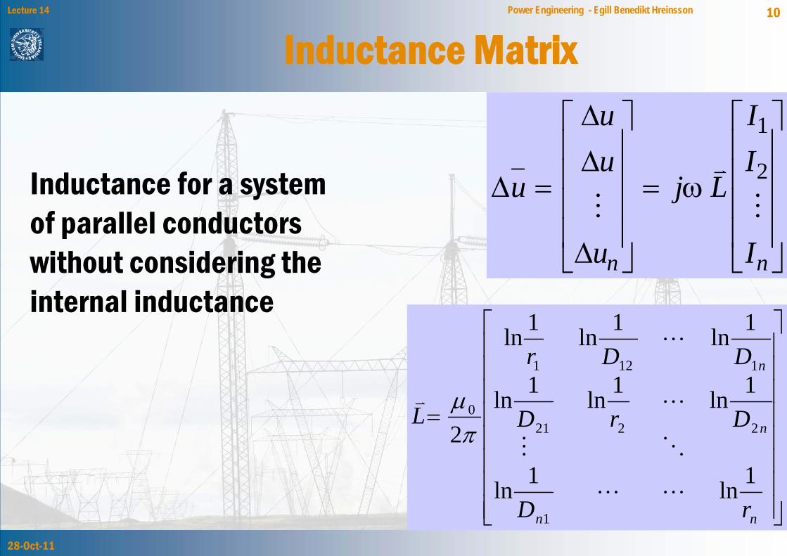
Inductance Matrix
Δ
ΔΔ
Δ
u
uu
u
j L
II
In n
=
⎡
⎣
⎢⎢⎢⎢
⎤
⎦
⎥⎥⎥⎥
=
⎡
⎣
⎢⎢⎢⎢
⎤
⎦
⎥⎥⎥⎥
ω
1
2
⎥⎥⎥⎥⎥⎥⎥⎥
⎦
⎤
⎢⎢⎢⎢⎢⎢⎢⎢
⎣
⎡
=
nn
n
n
rD
DrD
DDr
L
1ln1ln
1ln1ln1ln
1ln1ln1ln
2
1
2221
1121
0
πμ
Inductance for a system of parallel conductors without considering the internal inductance

28-Oct-11
11Lecture 14 Power Engineering - Egill Benedikt Hreinsson
Capacitance Matrix - Beta Matrix
1
1
111−=
⎥⎥⎥
⎦
⎤
⎢⎢⎢
⎣
⎡= β
nnn
n
CC
CCC
⎥⎥⎥
⎦
⎤
⎢⎢⎢
⎣
⎡== −
nnn
n
Cββ
βββ
1
1111
We can now compare the previous matrices regarding both inductance and capacitance. In both cases these matrices can not exist physically, although mathematically there is no problem. This is because each element in these matrices is a logarithm of a factor which has a dimension of m !!
28-Oct-11
12Lecture 14 Power Engineering - Egill Benedikt Hreinsson
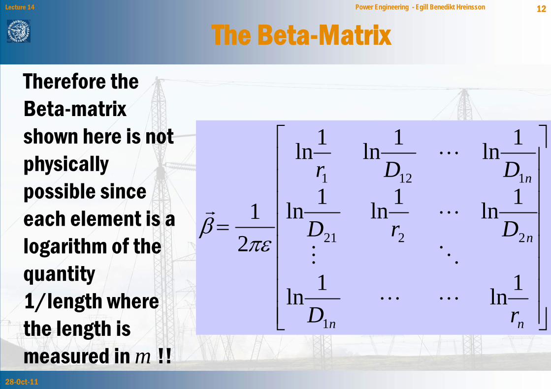
The Beta-Matrix
⎥⎥⎥⎥⎥⎥⎥⎥
⎦
⎤
⎢⎢⎢⎢⎢⎢⎢⎢
⎣
⎡
=
nn
n
n
rD
DrD
DDr
1ln1ln
1ln1ln1ln
1ln1ln1ln
21
1
2221
1121
πεβ
Therefore the Beta-matrix shown here is not physically possible since each element is a logarithm of the quantity 1/length where the length is measured in m !!

28-Oct-11
13Lecture 14 Power Engineering - Egill Benedikt Hreinsson
Capacitance - Inductance
1 2/ 2L C πε
μ π−= ⋅
2
1L C E Ec
με= ⋅ =
We now consider the product of these 2 matrices shown to the right. The result is that the product of the capacitance matrix and the inductance matrixis constant for a system of thin conductors
1 0
0 1is the unit matrixE
⎛ ⎞⎜ ⎟= ⎜ ⎟⎜ ⎟⎝ ⎠
…
28-Oct-11
14Lecture 14 Power Engineering - Egill Benedikt Hreinsson
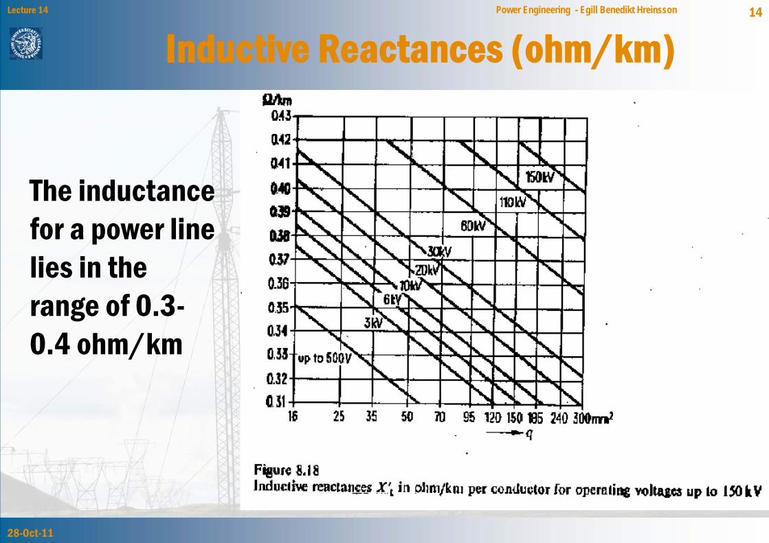
Inductive Reactances (ohm/km)
The inductance for a power line lies in the range of 0.3-0.4 ohm/km
28-Oct-11
15Lecture 14 Power Engineering - Egill Benedikt Hreinsson
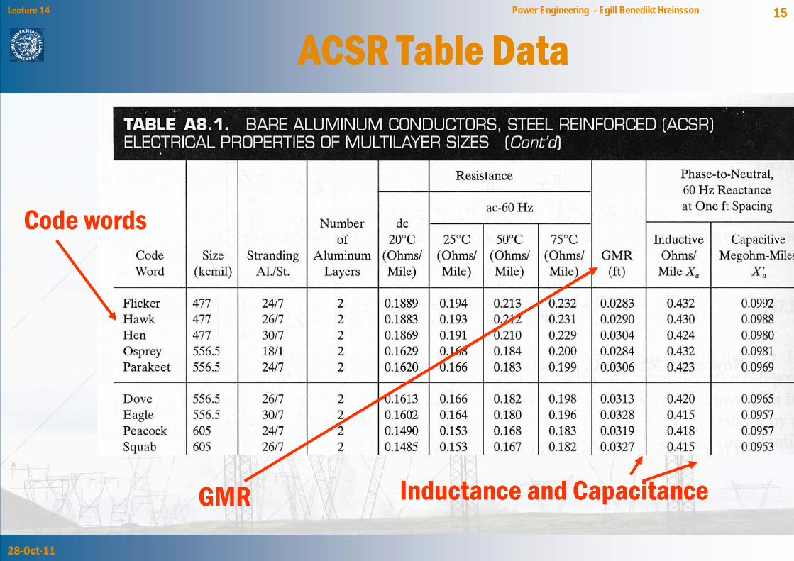
ACSR Table Data
Inductance and Capacitance GMR
Code words

28-Oct-11
16Lecture 14 Power Engineering - Egill Benedikt HreinssonTypical values of overhead linecharacteristics at 50 Hz
Typically for voltages below 60 kV line charging may be ignored. For extra high voltages (400 kV+) line charging must be carefully analyzed

28-Oct-11
17Lecture 14 Power Engineering - Egill Benedikt HreinssonTypical values for underground cablecharacteristics at 50 Hz
For underground cables SIL exceeds the thermal rating which means that underground cable connections are always net producers of reactive power

28-Oct-11
18Lecture 14 Power Engineering - Egill Benedikt Hreinsson
Capacitances (nF/km)

28-Oct-11
19Lecture 14 Power Engineering - Egill Benedikt Hreinsson
28-Oct-11
Additional Transmission topics• Ground wires: Transmission lines are usually
protected from lightning strikes with a ground wire. This topmost wire (or wires) helps to attenuate the transient voltages/currents that arise during a lighting strike. The ground wire is typically grounded at each pole.
• Corona discharge: Due to high electric fields around lines, the air molecules become ionized. This causes a crackling sound and may cause the line to glow!

28-Oct-11
20Lecture 14 Power Engineering - Egill Benedikt Hreinsson
Resistance of transmission linesand transmission real losses

28-Oct-11
21Lecture 14 Power Engineering - Egill Benedikt Hreinsson
Factor Influencing Line Resistance
• Skin effect (0-5%)• Temperature• Conductor winding (Spiraling effect ) (0-5%)
dcRAρ ⋅
=
Because ac current tends to flow towards the surface of a conductor, the resistance of a line at 60 Hz is slightly higher than at dc.Resistivity and hence line resistance increase as conductor temperature increases (changes is about 8% between 25°C and 50°C)
28-Oct-11
22Lecture 14 Power Engineering - Egill Benedikt Hreinsson
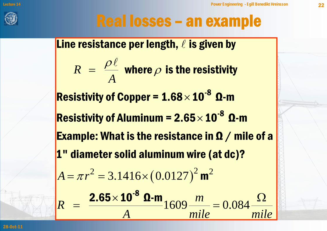
Real losses – an example
-8
-8
Line resistance per length, is given by
where is the resistivity
Resistivity of Copper = 1.68 10 Ω-m
Resistivity of Aluminum = 2.65 10 Ω-mExample: What is the resistance in Ω / mile of a
RAρ ρ=
×
×
( )22 23.1416 0.0127
1609 0.084-8
1" diameter solid aluminum wire (at dc)?
m
2.65 10 Ω-m
A r
mRA mile mile
π= = ×
× Ω= =
28-Oct-11
23Lecture 14 Power Engineering - Egill Benedikt Hreinsson
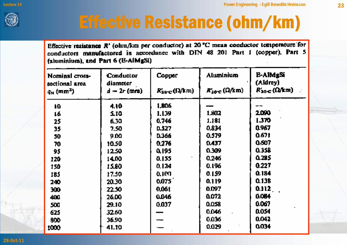
Effective Resistance (ohm/km)

28-Oct-11
24Lecture 14 Power Engineering - Egill Benedikt Hreinsson
Circuit models for short transmission lines
Transmission Capacity

28-Oct-11
25Lecture 14 Power Engineering - Egill Benedikt Hreinsson
One phase equivalent model for a short line
C/2
R+jXi j
C/2
28-Oct-11
26Lecture 14 Power Engineering - Egill Benedikt Hreinsson
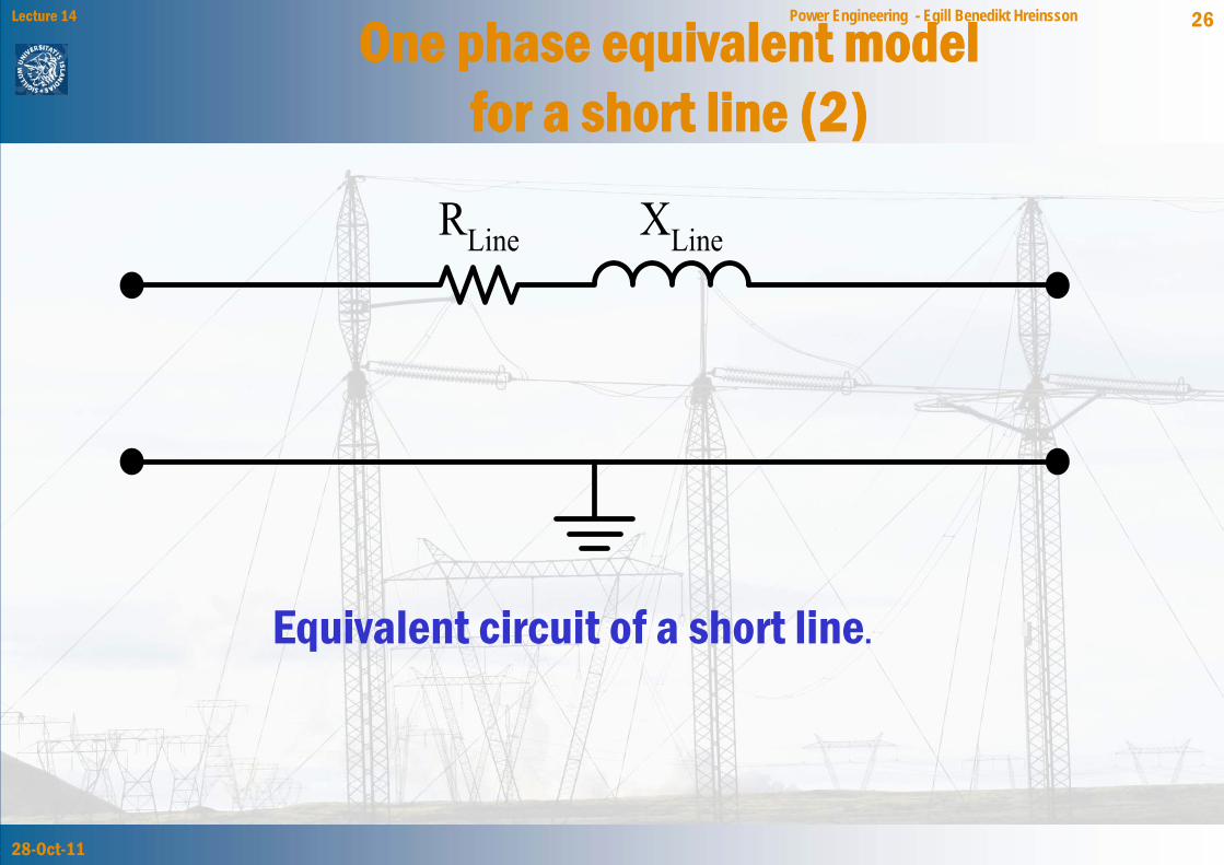
Equivalent circuit of a short line.
One phase equivalent model for a short line (2)

28-Oct-11
27Lecture 14 Power Engineering - Egill Benedikt Hreinsson
One phase equivalent model for a long line
Sendingend
Receivingend
···
Equivalent circuit for a long transmission line.

28-Oct-11
28Lecture 14 Power Engineering - Egill Benedikt Hreinsson
One phase equivalent model for a long line (3)
Sendingend
Receivingend
···
Equivalent circuit for a long transmission line.
•Series L draws reactive power•QL=wLI2 – decreases V along line
•Line charging C generatesreactive power
•QC=wCV2 – increases V along line

28-Oct-11
29Lecture 14 Power Engineering - Egill Benedikt Hreinsson
Voltage balance along the line• QL << QC
– Light load – voltage increases along line• QL >> QC
– Heavy load – voltage decreases
V1
V(x)
x
Light
Heavy
What happens if: QL = QC ?
28-Oct-11
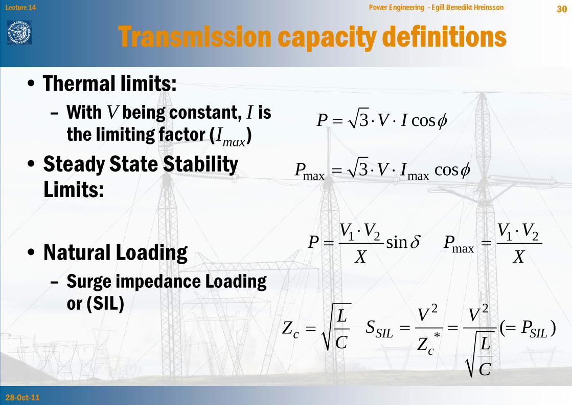
30Lecture 14 Power Engineering - Egill Benedikt Hreinsson
Transmission capacity definitions• Thermal limits:
– With V being constant, I is the limiting factor (Imax)
• Steady State Stability Limits:
• Natural Loading – Surge impedance Loading
or (SIL)
1 2 sinV VPX
δ⋅
=
3 cosP V I φ= ⋅ ⋅
1 2max
V VPX⋅
=
cLZC
=2 2
* ( )SIL SILc
V VS PLZC
= = =
max max3 cosP V I φ= ⋅ ⋅

28-Oct-11
31Lecture 14 Power Engineering - Egill Benedikt Hreinsson
Surge Impedance Loading (SIL)
• SIL is reached, when the generated reactive power equals the consumed power in the high voltage line.
• SIL is not maximum loading but a “characteristic loading”
2 2consumed LQ X I L Iω= =
2 22
1generatedc
V VQ C V
X Cω
ω= = =
2 2
generated consumedQ Q
L I C Vω ω
=
=
c
XLZC C
ω= =
22
2 cV L Z
CI= =

28-Oct-11
32Lecture 14 Power Engineering - Egill Benedikt Hreinsson
Surge Impedance Loading• Surge Impedance:
– Also called characteristic impedance. this is the impedance with which you can insert a surge the sending end of the line and not get any reflection back at the receiving end.
• X is the reactance of the line
– (in Ohm/km or in Ohm)• B is the succeptance of the
line – (in Siemens/km or in
Siemens)
Surge impedance
Receiving end
Sending end
c
XL XZC C B
ω= = = (≅ 250 – 400 ohm)
C/2
R+jXi j
C/2
28-Oct-11
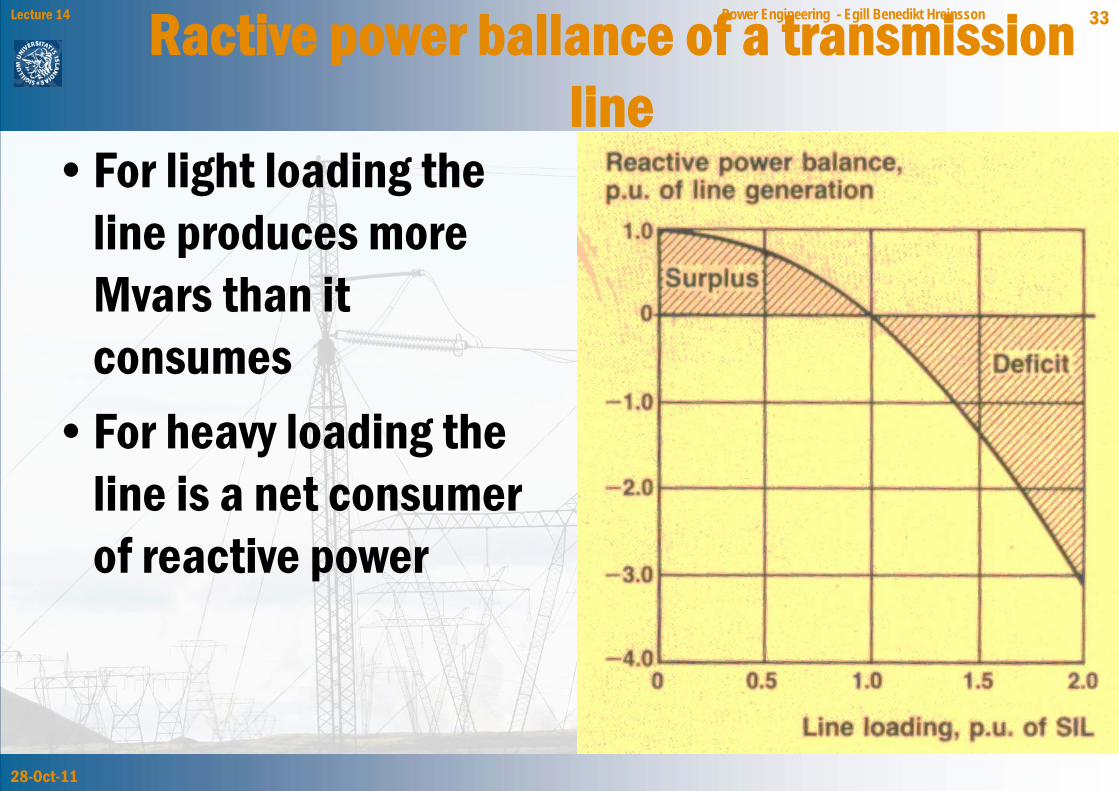
33Lecture 14 Power Engineering - Egill Benedikt HreinssonRactive power ballance of a transmission line
•For light loading the line produces more Mvars than it consumes
•For heavy loading the line is a net consumer of reactive power


