Calculus II Workbook Note to Students: This workbook contains examples and exercises that will be referred to regularly during class. Please purchase or print out the rest of the workbook before our next class and bring it to class with you every day. Please note that you will need extra loose leaf paper to do some of the exercises in this workbook. 1. To Purchase the Workbook. Go to the Copy Corner on the ground floor of the Student Union during their business hours (Monday - Thursday, 8:30 a.m. to 6:30 p.m. or Friday, 8:30 a.m. to 4:30 p.m.). Ask for a copy of the Math 211 Workbook. The copying charge will probably be between $5.00 and $10.00. 2. To Print Out the Workbook. Go to the web address below http://www.sonoma.edu/users/l/lahme/m211/ and click on the link “Math 211 Workbook”, which will open the file containing the workbook as a .pdf file. BE FOREWARNED THAT THERE ARE LOTS OF PICTURES AND MATH FONTS IN THE WORKBOOK, SO SOME PRINTERS MAY NOT BE ABLE TO HANDLE THE JOB OF PRINTING THIS ITEM, ESPECIALLY IF THEY ARE OLD, SLOW, OR NOT INTENDED FOR HEAVY DUTY JOBS. If you do choose to try to print it, please leave yourself enough time to purchase the workbook before Thursday’s class in case your printing attempt is unsuccessful.
Transcript
Calculus II Workbook
Note to Students: This workbook contains examples and exercises that
will be referred to regularly during class. Please purchase or print out the rest
of the workbook before our next class and bring it to class with you every
day. Please note that you will need extra loose leaf paper to do some of the
exercises in this workbook.
1. To Purchase the Workbook. Go to the Copy Corner on the ground floor of the Student Unionduring their business hours (Monday - Thursday, 8:30 a.m. to 6:30 p.m. or Friday, 8:30 a.m. to 4:30p.m.). Ask for a copy of the Math 211 Workbook. The copying charge will probably be between $5.00and $10.00.
2. To Print Out the Workbook. Go to the web address below
http://www.sonoma.edu/users/l/lahme/m211/
and click on the link “Math 211 Workbook”, which will open the file containing the workbook as a.pdf file. BE FOREWARNED THAT THERE ARE LOTS OF PICTURES AND MATH FONTSIN THE WORKBOOK, SO SOME PRINTERS MAY NOT BE ABLE TO HANDLE THE JOB OFPRINTING THIS ITEM, ESPECIALLY IF THEY ARE OLD, SLOW, OR NOT INTENDED FORHEAVY DUTY JOBS. If you do choose to try to print it, please leave yourself enough time to purchasethe workbook before Thursday’s class in case your printing attempt is unsuccessful.
Section 5.5 – The Substitution Rule (Review from Calculus I)
The Substitution Rule. Under “nice” conditions (see formulas 4 and 5 in the text for the precisestatement of the conditions), we can choose u = g(x) to obtain the following formulas:
1.
∫
f(g(x))g′(x) dx =
∫
f(u) du
2.
∫ b
a
f(g(x))g′(x) dx =
∫ u(b)
u(a)
f(u) du
Comments on the Substitution Rule:
1. When making a substitution, the goal is to transform an existing integral into an easier integral that we canthen evaluate.
2. While there is no set method that will always work when it comes to choosing your u, here are someguidelines that will often work:
(a) Choose “u” so that “du” appears somewhere in your integrand.
(b) Choose “u” to be the “inside” portion of some composite function.
Example. Calculate
∫
x sin(x2 + 5) dx.
Exercises
For problems 1-9, evaluate each of the following integrals. Keep in mind that using a substitution may not work onsome problems.
1.
∫
sinx cos2 xdx
2.
∫ 3
1
e1/x
x2dx
3.
∫
1
1 + 4x2dx
4.
∫
tanxdx
5.
∫
x√1 − x
dx
6.
∫ 4
1
2x − 3
x2dx
7.
∫ 2
0
ex
ex + 1dx
8.
∫ 2
0
ex + 1
exdx
9.
∫
ax dx Hint: ax = ex ln a
Math 211 Workbook 4
Section 5.6 – Integration by Parts
Recall the Product Rule for differentiation:
d
dx[u(x)v(x)] =
Integration by Parts Formula.
Examples:
1.
∫
x cosxdx
Math 211 Workbook 5
2.
∫
x lnxdx
Notes on Integration by Parts:
1. “u” and “dv” together must give everything inside your original integral. The “dv” part will containthe differential from your original integral.
2. If possible, we choose u and dv so that the integral∫
v du can be evaluated directly. Otherwise, we tryto choose u and dv so that
∫
v du is simpler than the integral we started with.
3. General Rule. Choose dv to be the largest portion of the original integral that you can find anantiderivative for. This rule won’t always work, but will help guide you to a good choice in many cases.
Exercises
Evaluate each of the following integrals.
1.
∫
xex dx
2.
∫
x2e2x dx
3.
∫ e
1
lnxdx
4.
∫
x5ex3
dx
5.
∫
arcsinxdx
6.
∫
ex sinxdx
Math 211 Workbook 6Section 5.7 – Other Integration Techniques
Example 1. Calculate
∫
sin3 xdx.
Example 2. Calculate
∫
cos5 x sin2 xdx.
Example 3. Calculate
∫
sin2 xdx.
Math 211 Workbook 7
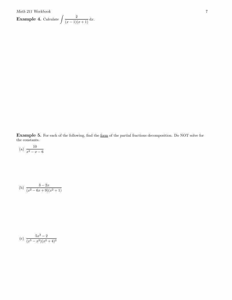
Example 4. Calculate
∫
2
(x − 1)(x + 1)dx.
Example 5. For each of the following, find the form of the partial fractions decomposition. Do NOT solve forthe constants.
(a)10
x2 − x − 6
(b)3 − 2x
(x2 − 6x + 9)(x2 + 1)
(c)5x3 − 2
(x5 − x3)(x2 + 4)2
Math 211 Workbook 8
Section 5.7 Information
Integrating Powers of Sine and Cosine:∫
cosm x sinn xdx
Case 1. If m is odd, “steal” a power from cosx and let u = sin x.
Case 2. If n is odd, “steal” a power from sinx and let u = cosx.
Case 3. If both m and n are even, you will need to use the identity sin2 x = 12 (1 − cos(2x)) and/or the
identity cos2 x = 12 (1 + cos(2x)).
Partial Fractions for Integrating Rational Functions.∫
P (x)
Q(x)dx,
where P (x) and Q(x) are polynomials.
Case 1. P (x) has lower degree than Q(x). In this case, formulate your partial fractions decomposition assuggested below.
Type of Factor in Q(x) Corresponding Term(s) in Partial Fraction Decomposition
Linear: mx + nA
mx + n
Repeated
Linear: (mx + n)k A1
mx + n+
A2
(mx + n)2+ · · · + Ak
(mx + n)k
Irreducible
Quadratic: mx2 + nx + rAx + B
mx2 + nx + r
Repeated Irreducible
Quadratic: (mx2 + nx + r)k A1x + B1
mx2 + nx + r+
A2x + B2
(mx2 + nx + r)2+ · · · + Akx + Bk
(mx2 + nx + r)k
Case 2. P (x) has equal or greater degree than Q(x). In this case, long division must be used first, and thenCase 1 must be applied to the remainder term.
Exercises
1. Calculate each of the following:
(a)
∫
cos9 x sin3 xdx
(b)
∫
2x2 + 4x − 9
x3 + 9xdx
(c)
∫
14x2 − 17x + 1
x(2x − 1)2dx
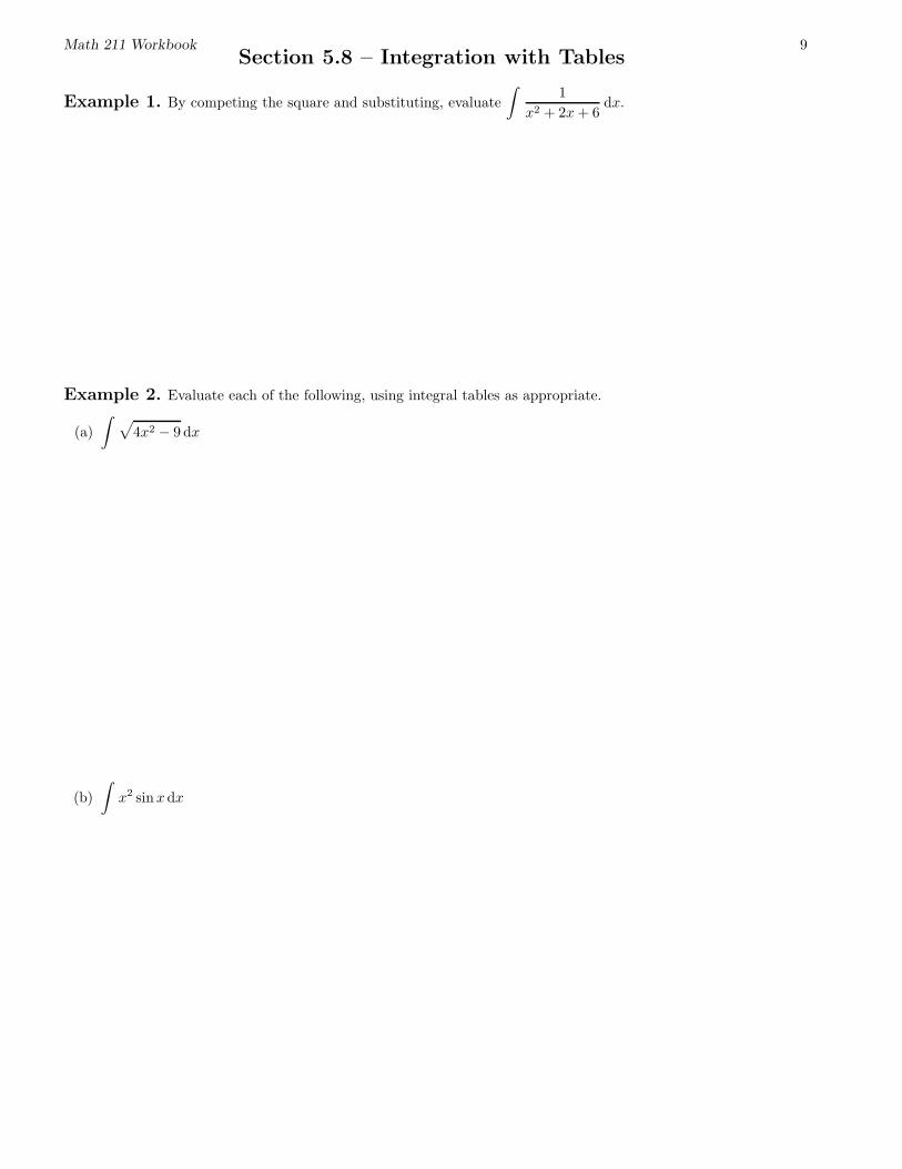
Math 211 Workbook 9Section 5.8 – Integration with Tables
Example 1. By competing the square and substituting, evaluate
∫
1
x2 + 2x + 6dx.
Example 2. Evaluate each of the following, using integral tables as appropriate.
(a)
∫
√
4x2 − 9 dx
(b)
∫
x2 sin xdx
Math 211 Workbook 10
Examples and Exercises
1. Evaluate each of the following, using integral tables where appropriate.
(a)
∫
cos3(4x) dx
(b)
∫
e5x sin(3x) dx
(c)
∫
ex√
1 + 2ex dx
(d)
∫
√
11 − 6x − x2 dx
(e)
∫
3x3 + x2 + 30x + 13
x2 + 9dx
Math 211 Workbook 11
Section 5.9 – Numerical Integration
1. The Trapezoidal Rule
∆x = width of one subdivisionn = number of subdivisions
=ba= x0 x1 x2 n−1x xxn
Tn = approximation of
∫ b
a
f(x) dx using n subdivisions
=
2. The Midpoint Rule
∆x = width of one subdivisionn = number of subdivisions
=ba= x0 x1 x2 n−1x xxn
Mn =
Math 211 Workbook 12
Error Bound Theorems
Let f(x) be an integrable function on [a, b], and let |f ′′(x)| ≤ K on [a, b]. The chart below gives the maximum
possible error in the approximation of
∫ b
a
f(x) dx using various numerical integration techniques.
Approximation Method Maximum Possible Error
Trapezoid RuleK(b − a)3
12n2
Midpoint RuleK(b − a)3
24n2
Examples and Exercises
1. Let f(x) = e−x2
.
(a) Use the Midpoint Rule and the Trapezoidal Rule, both with n = 4, to find two estimates of
∫ 1
0
e−x2
dx.
Math 211 Workbook 13
(b) Use the graph of f ′′(x) given to the right to find the max-imum possible error in your estimates from part (a).
f ′′(x)
0.2 0.4 0.6 0.8 1
-3
-2.5
-2
-1.5
-1
-0.5
0.5
1
(c) How large must n be taken in the Midpoint Rule to guarantee an error of less than 0.000001 from thetrue value of the integral?
2. Given to the right is the graph of a function g(x) (solidgraph) and g′′(x) (dotted graph). Use the Trapezoidal rule
with n = 4 to estimate the value of
∫ 2
0
g(x) dx. What is
the maximum possible error in your estimate? 0.5 1 1.5 2
-3
-2
-1
1
2
Math 211 Workbook 14
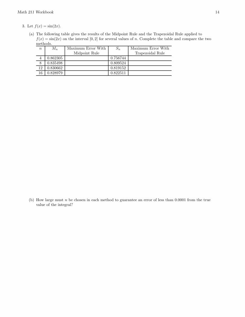
3. Let f(x) = sin(2x).
(a) The following table gives the results of the Midpoint Rule and the Trapezoidal Rule applied tof(x) = sin(2x) on the interval [0, 2] for several values of n. Complete the table and compare the twomethods.
n Mn Maximum Error With Sn Maximum Error WithMidpoint Rule Trapezoidal Rule
(b) How large must n be chosen in each method to guarantee an error of less than 0.0001 from the truevalue of the integral?
Math 211 Workbook 15
Section 6.1 – Area Between Curves
Goal. Find the area between the functions y = f(x) and y = g(x) on the interval a ≤ x ≤ b.
y=g(x)
a bx x xx = =x0 1 2 3 n
y=f(x)
y=g(x)
a b
y=f(x)
Example 1. Find the area bounded between y =√
x and y = x2
8 .
Math 211 Workbook 16
Example 2. Find the area between y = sin x and y = cosx on the interval [0, π2 ].
Example 3. Find the area of the region bounded by the curves x = 1−y4
and x = y3 − y (see diagram to the right).
x
y
Math 211 Workbook 17
Example 4. Consider the region bounded by the curvesy2 = 2x+6 and x− y = 1 shown to the right. Set up inte-grals that represent the area of this region in two differentways: (1) Integrate in the x-direction, (2) Integrate in they-direction. Then, calculate the area of the region.
-4 -3 -2 -1 1 2 3 4 5 6
-5
-4
-3
-2
-1
1
2
3
4
5
Math 211 Workbook 18
Section 6.2 – Volume
Preliminary Example. Colonel Armstrong is a 1300 year old Redwoodtree whose trunk is 300 feet tall. Every 60 feet, a diameter measurement ofColonel Armstrong has been taken (see diagram to right). Use this informa-tion to estimate the volume of wood in Colonel Armstrong’s trunk.
9ft
300 ft
8ft
8ft
10 ft
12 ft
14 ft
Math 211 Workbook 19
Example 1. Find the volume of the solid region generated by rotating the curve y = sin x about the x-axis onthe interval [0, π].
Example 2. Find the volume of the solid region generated by rotating the region bounded by y = 2, x = 0, andy = 3
√x about the x-axis.
Math 211 Workbook 20
Example 3. Set up, but DO NOT EVALUATE, an integral that gives the volume of the solid region generatedby rotating the region bounded between y = x and y = x2 about the line x = 2.
Exercises
1. Consider the figure given to the right. For each of thefollowing, set up, but do not evaluate, an integral thatrepresents the volume obtained when the specified regionis rotated around the given axis.
3
(8,2)
(0,0)
(0,2)
(8,0)x=4y
y=x1/3
R
RR
1
2
(a) R1 about the x-axis.
(b) R1 about the y-axis.
(c) R2 about the x-axis.
(d) R2 about the y-axis.
(e) R2 about the line x = 9.
(f) R3 about the line y = 3.
2. Find the volume of a pyramid whose base is a square withside L and whose height is h. This solid region is pictured(on its side) to the right. Notice that a suggestive slice hasbeen drawn in for you.
Physical Situation An object is taken out of an oven and placed in a room wherethe temperature is 75◦F. Let T (t) represent the temperature of theobject, in ◦F, after t minutes.
Modeling Differential EquationdT
dt= k(75 − T ), where k > 0 is a constant.
Description of the Physical Law Modeledby the Differential Equation
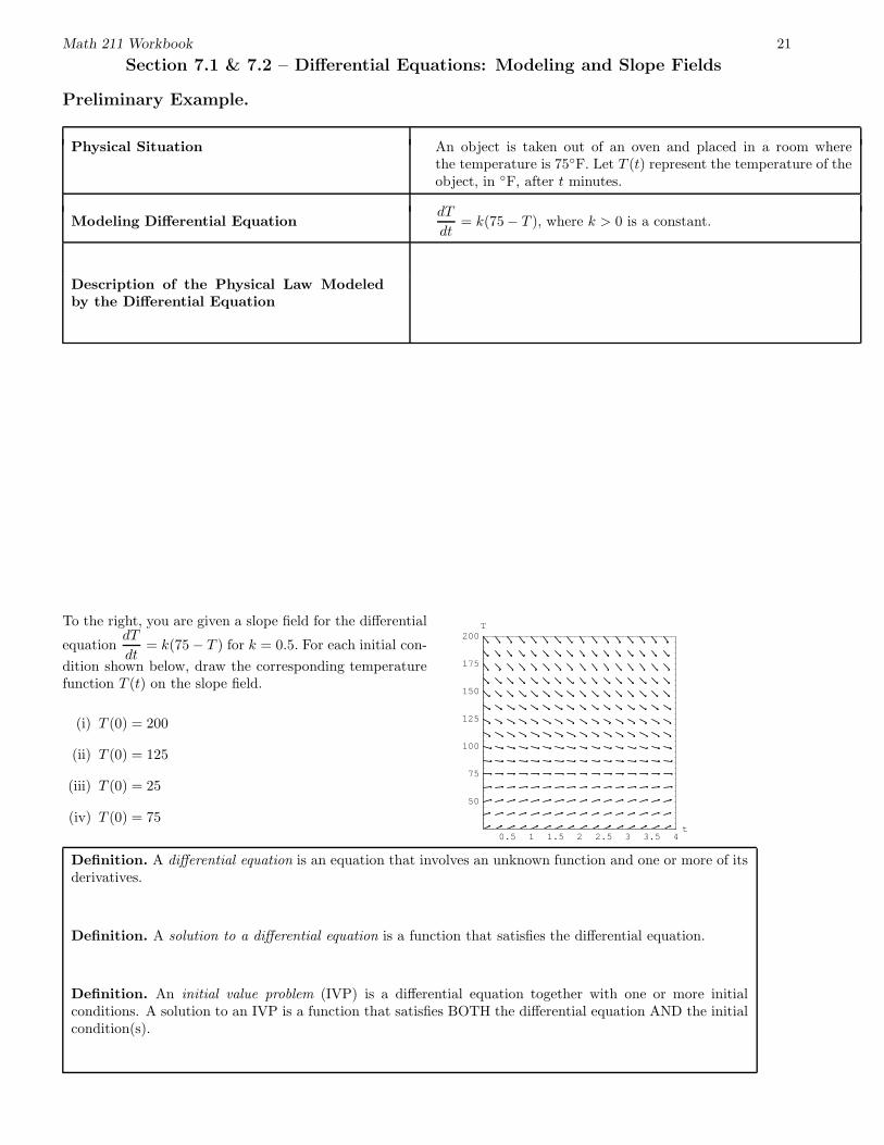
To the right, you are given a slope field for the differential
equationdT
dt= k(75 − T ) for k = 0.5. For each initial con-
dition shown below, draw the corresponding temperaturefunction T (t) on the slope field.
(i) T (0) = 200
(ii) T (0) = 125
(iii) T (0) = 25
(iv) T (0) = 750.5 1 1.5 2 2.5 3 3.5 4
50
75
100
125
150
175
200
t
T
Definition. A differential equation is an equation that involves an unknown function and one or more of itsderivatives.
Definition. A solution to a differential equation is a function that satisfies the differential equation.
Definition. An initial value problem (IVP) is a differential equation together with one or more initialconditions. A solution to an IVP is a function that satisfies BOTH the differential equation AND the initialcondition(s).
Math 211 Workbook 22
Example 1. Let y(t) represent the percentage of a particular task that has been learned after t months. Then ycan be modeled using the differential equation dy
dt = k(100 − y), where k is a positive constant.
(a) The slope field to the right represents the differential equa-tion given above with k = 0.2. Draw in the solutions to thefollowing initial value problems:
(i) dydt = 0.2(100− y), y(0) = 20
(ii) dydt = 0.2(100− y), y(0) = 60
(b) Who learns faster at the beginning, a person who starts outknowing 20% of a task or a person who starts out knowing60% of a task? Explain.
2 4 6 8 10 12
20
40
60
80
100
t
y
(c) Explain, in the context of this situation, what the modeling differential equation dydt = k(100 − y) is saying.
Example 2. Let P (t) represent the population of a bacteria colony after t hours. Assume that this population ismodeled by the differential equation dP
dt = 0.3P, whose slope field is given below
(a) Draw in the solutions to the following initial value prob-lems:
(i) dPdt = 0.3P, P (0) = 100
(ii) dPdt = 0.3P, P (0) = 200
(b) Estimate the amount of time it takes for the population ofa bacteria colony to double if it starts with 200 bacteria.
1 2 3 4 5 6
100
200
300
400
500
t
y
Math 211 Workbook 23
(c) For each of the following functions, use the slope field to guess whether the function could be a solution to thedifferential equation dP
dt = 0.3P. Then, use algebra and calculus to confirm your guesses.
(i) P = e0.3t
(ii) P = 100e0.3t
(iii) P = t + 100
(iv) P = e0.3t+4
(v) P = 0
(vi) P = 200 sin t
Exercises
1. Let k and C be any constants. Consider the differential equations given below:
(I)dx
dt= 2x (II) x′′ = −x
For each of the functions given below, decide whether the function is a solution to (I), to (II), or to both (I)and (II).
(a) x = Ce2t (b) x = 2 cos t (c) x = 3 cos t − 4 sin t (d) x = 0
Math 211 Workbook 24
2. (a) Show that all members of the family y =1√
c − x2are solutions of the differential equation y′ = xy3.
(b) Use part (a) to find a formula for the solution to the ini-tial value problem y′ = xy3, y(0) = 2. Then, sketch yoursolution on the slope field shown to the right.
-0.75-0.5-0.25 0 0.25 0.5 0.75 1
0.5
1
1.5
2
2.5
3
3.5
4
t
y
Figure 1. Slope field for y′ = xy3
3. (a) Show that all members of the family y = x3 +c
x2are solutions of the differential equation xy′ = 5x3−2y.
(b) Find the solution to the initial value problem xy′ = 5x3 − 2y, y(1) = 5.
4. For what nonzero values of k does the function y = ekt solve the differential equation y′′ − y′ − 6y = 0?
5. (Taken from Stewart) A population is modeled by the differential equationdP
dt= 1.2P
(
1 − P
4200
)
.
(a) For what values of P is the population increasing?
(b) For what values of P is the population decreasing?
6. Below, you are given 8 differential equations. Match each differential equation with the appropriate directionfield (given on the next page). Then, complete parts (a)–(c) below.
(I) y′ = 1 (II) y′ = y (III) y′ = x − y (IV) y′ = cos(x)
(a) For each of the direction fields, draw in the solution that satisfies the initial condition y(0) = 1.
(b) Can you guess a formula for any of the solutions you drew in for part (a)? Check to see if you’re right!
Definition. A constant solution to a differential equation is called an equilibrium solution. Graphically,an equilibrium solution is a horizontal line, that is, a solution of the form y = c for some constant c.
7. Use the above definition of equilibrium solution to answer the following:
(a) Does the differential equation from the Preliminary Example a few pages ago have any equilibriumsolutions? If so, what are they?
(b) Does the differential equation from Example 2 (preceding the exercises) have any equilibrium solutions?If so, what are they?
(c) Does the differential equation from Exercise 5 above have any equilibrium solutions? If so, what arethey?
(d) Which of the differential equations from Exercise 6 above have an equilibrium solution? For those thatdo, what are the equilibrium solutions?
Math 211 Workbook 25
-3 -2 -1 0 1 2 3
-3
-2
-1
0
1
2
3
x
y
-3 -2 -1 0 1 2 3
-3
-2
-1
0
1
2
3
x
y
-3 -2 -1 0 1 2 3
-3
-2
-1
0
1
2
3
x
y
-3 -2 -1 0 1 2 3
-3
-2
-1
0
1
2
3
x
y
-3 -2 -1 0 1 2 3
-3
-2
-1
0
1
2
3
x
y
-3 -2 -1 0 1 2 3
-3
-2
-1
0
1
2
3
x
y
-3 -2 -1 0 1 2 3
-3
-2
-1
0
1
2
3
x
y
-3 -2 -1 0 1 2 3
-3
-2
-1
0
1
2
3
x
y
Math 211 Workbook 26
Euler’s Method
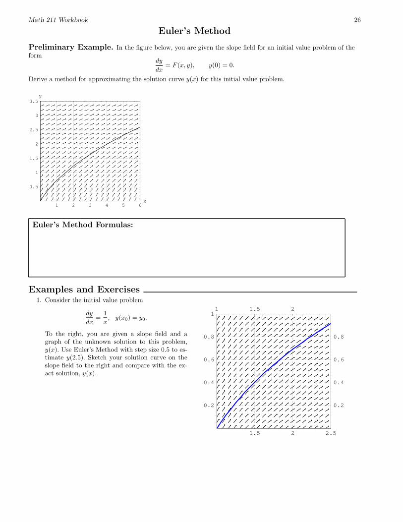
Preliminary Example. In the figure below, you are given the slope field for an initial value problem of theform
dy
dx= F (x, y), y(0) = 0.
Derive a method for approximating the solution curve y(x) for this initial value problem.
1 2 3 4 5 6
0.5
1
1.5
2
2.5
3
3.5
x
y
Euler’s Method Formulas:
Examples and Exercises1. Consider the initial value problem
dy
dx=
1
x, y(x0) = y0.
To the right, you are given a slope field and agraph of the unknown solution to this problem,y(x). Use Euler’s Method with step size 0.5 to es-timate y(2.5). Sketch your solution curve on theslope field to the right and compare with the ex-act solution, y(x).
1.5 2 2.5
0.2
0.4
0.6
0.8
11 1.5 2
0.2
0.4
0.6
0.8
Math 211 Workbook 27
2. The slope field for the differential equation
y′ − y = x
is shown to the right. Use Euler’s method to ap-proximate solution curves to the following initialvalue problems:
(a) y′ − y = x, y(−1) = 0
(b) y′ − y = x, y(−1) = 0.5
Use a step size of 0.5 in both cases.
-1.5 -1 -0.5 0 0.5 1 1.5 2
-1.5
-1
-0.5
0
0.5
1
1.5
2
x
y
Math 211 Workbook 28
Section 7.3 – Separable Equations
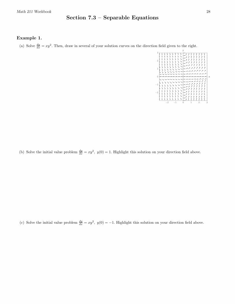
Example 1.
(a) Solve dydx = xy2. Then, draw in several of your solution curves on the direction field given to the right.
-2 -1 0 1 2 3
-2
-1
0
1
2
3
x
y
(b) Solve the initial value problem dydx = xy2, y(0) = 1. Highlight this solution on your direction field above.
(c) Solve the initial value problem dydx = xy2, y(0) = −1. Highlight this solution on your direction field above.
Math 211 Workbook 29
Example 2. For each of the following, you are given a differential equation, a slope field, and an initial valueproblem. First, solve the differential equation and draw in several of your solution curves. Then, solve the initialvalue problem and highlight this particular solution curve.
(i) dydx = y
(ii) dydx = y, y(0) = 2
-2 -1 0 1 2 3
-2
-1
0
1
2
3
x
y
(i) dydx = 1/y
(ii) dydx = 1/y, y(0) = 1
-2 -1 0 1 2 3
-2
-1
0
1
2
3
x
y
Math 211 Workbook 30
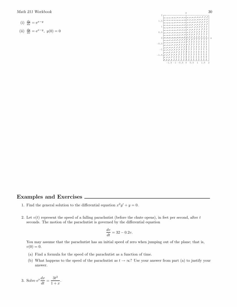
(i) dydx = ex−y
(ii) dydx = ex−y, y(0) = 0
-1.5 -1 -0.5 0 0.5 1 1.5 2
-1.5
-1
-0.5
0
0.5
1
1.5
2
x
y
Examples and Exercises
1. Find the general solution to the differential equation x2y′ + y = 0.
2. Let v(t) represent the speed of a falling parachutist (before the chute opens), in feet per second, after tseconds. The motion of the parachutist is governed by the differential equation
dv
dt= 32 − 0.2v.
You may assume that the parachutist has an initial speed of zero when jumping out of the plane; that is,v(0) = 0.
(a) Find a formula for the speed of the parachutist as a function of time.
(b) What happens to the speed of the parachutist as t → ∞? Use your answer from part (a) to justify youranswer.
3. Solve ex dx
dt=
3t2
1 + x.
Math 211 Workbook 31
Section 7.4 – Exponential Growth and Decay
Preliminary Example. A quantity that obeys the law of natural growth (or decay) behaves in the followingway: the rate at which the quantity grows (or decays) is proportional to the amount of the quantity present at anygiven time. If y(t) represents the amount of such a quantity present at time t, write down a modeling differentialequation for y.
Some quantities that obey the law of natural growth (or decay)
Example 1. A bacteria colony starts with 700 bacteria and grows at a rate proportional to its size. After 4hours there are 2100 bacteria.
(a) Find an expression for the number of bacteria after t hours.
(b) How many bacteria are there after 3 hours?
Math 211 Workbook 32
(c) How fast is the population growing after 3 hours?
Definition. The half-life of a radioactive substance is the amount of time that it takes for
Examples and Exercises
1. A 2-pound loaf of Wonderr bread has a half life of 6 months.
(a) How much bread is left after 3 months?
(b) How long until only 0.2 pound remains?
2. What is the half life of a radioactive substance that decays to 70% of its original mass in 20 years?
3. (Taken from Stewart) Newton’s Law of Cooling states that the rate of cooling of an object is proportional tothe temperature difference between the object and its surroundings. Suppose that a roast turkey is taken froman oven when its temperature has reached 185◦F and is placed on a table in a room where the temperature is75◦F. If u(t) is the temperature of the turkey after t minutes, then Newton’s Law of Cooling implies that
du
dt= k(u − 75).
(a) If the temperature of the turkey is 150◦F after half an hour, what is the temperature after 45 minutes?
(b) When will the turkey have cooled to 100◦F?
4. Show that the half life a radioactive substance is given by − ln 2/k, where k is the constant in the governingdifferential equation dq/dt = kq.
Math 211 Workbook 33
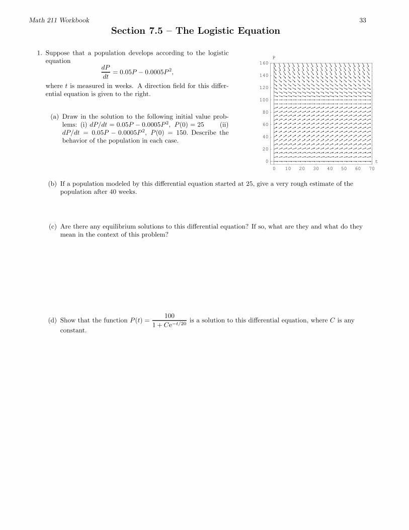
Section 7.5 – The Logistic Equation
1. Suppose that a population develops according to the logisticequation
dP
dt= 0.05P − 0.0005P 2,
where t is measured in weeks. A direction field for this differ-ential equation is given to the right.
(a) Draw in the solution to the following initial value prob-lems: (i) dP/dt = 0.05P − 0.0005P 2, P (0) = 25 (ii)dP/dt = 0.05P − 0.0005P 2, P (0) = 150. Describe thebehavior of the population in each case.
0 10 20 30 40 50 60 70
0
20
40
60
80
100
120
140
160
t
P
(b) If a population modeled by this differential equation started at 25, give a very rough estimate of thepopulation after 40 weeks.
(c) Are there any equilibrium solutions to this differential equation? If so, what are they and what do theymean in the context of this problem?
(d) Show that the function P (t) =100
1 + Ce−t/20is a solution to this differential equation, where C is any
constant.
Math 211 Workbook 34
(e) Use the result of part (d) to find exact solutions to the initial value problems from part (a) and an exactanswer to the question asked in part (b).
Definition. A differential equation that can be written in the form
dP
dt= kP
(
1 − P
K
)
,
where k and K are constants, is called a logistic differential equation.
Notes.
1. Logistic differential equations are often used to model population growth. The constant K is called thecarrying capacity of the population.
2. Using separation of variables, it can be shown that the general solution to the above logistic differential
equation is given by P (t) =K
1 + Ae−kt, where A is any constant. See our text, pp. 538-539, for details.
Math 211 Workbook 35
Section 5.10 – Improper Integrals
Preliminary Example. To theright, you are given the graphs ofy = 1/x4 and y = 1/x. Calculate the
“improper integrals”
∫
∞
1
1
x4dx and
∫
∞
1
1
xdx.
1
Figure 1. Graph of y = 1/x4
1
Figure 2. Graph of y = 1/x
Types of Improper Integrals
Improper Integral Definition Picture
∫
∞
a
f(x) dx =
a
∫ b
−∞
f(x) dx =
b
Math 211 Workbook 36
Improper Integral Definition Picture
∫
∞
−∞
f(x) dx =
∫ b
a
f(x) dx =
a b
∫ b
a
f(x) dx =
a b
∫ b
a
f(x) dx =
ca b
Definition. We say that an improper integral if all of the defining limitsexist and are finite. If any of the involved limits is infinite or does not exist, we say that the improper integral
.
Comparison Theorem. Suppose that f and g are contin-uous functions with f(x) ≥ g(x) ≥ 0 for x ≥ a.
1. If is convergent, then
is convergent.
2. If is divergent, then
is divergent. a
f(x)g(x)
Math 211 Workbook 37
Example 1. Consider the integral
∫ 1
−1
13√
x4dx.
(a) Explain why the above integral is improper.
(b) Determine whether or not this integral converges. If it does converge, find its value.
Example 2. Determine whether or not
∫ 1
0
x lnxdx converges. If it does converge, find its value.
Math 211 Workbook 38
Examples and Exercises
1. Determine whether or not
∫
∞
1
lnx
x2dx converges. If it does converge, find its value.
2. Use the Comparison Theorem to determine whether or not the integral
∫
∞
1
1
x4 + 1dx converges.
Note: On a problem like #2 above where you’re being asked to use a theorem to justify a conclusion, youare, in effect, being asked to write a proof. This means that explanations must be written in clear, completesentences in order to receive credit. On such a problem, it is your job to convince the reader that yourargument makes sense, and not the reader’s job to figure out what you mean.
3. Use the relevant facts in the following theorem to answer each of the questions that follow. Justify youranswers with complete explanations, using the note following exercise 2 above as a guideline.
Theorem.
(A)
∫
∞
1
1
xpdx is convergent if p > 1 and divergent if p ≤ 1.
(B)
∫
∞
1
1
erxdx is convergent if r > 0 and divergent if r ≤ 0.
(a) Does
∫
∞
2
1√x − 1
dx converge or diverge?
(b) Does
∫
∞
1
1
x + x6dx converge or diverge?
(c) Does
∫
∞
2
e−x2
dx converge or diverge?
4. Is the solution to the problem below correct or incorrect? Explain.
Problem. Determine whether
∫
∞
2
1√x + 1
dx converges or diverges.
Solution. Since for all x ≥ 1, the denominator of1√
x + 1is bigger than the denominator of
1√x
. This means that
0 ≤ 1√x + 1
≤ 1√x
for all x ≥ 1.
Therefore, since
∫
∞
2
1√x
dx diverges by fact (i) from the previous page,
∫
∞
2
1√x + 1
dx must
also diverge by the Comparison Theorem.
Math 211 Workbook 39
Sequences and Series – An Introduction
Example. The Cantor Set is obtained by starting with the interval [0, 1], then removing the numbers in(1/3, 2/3) (i.e. removing the “middle third” of the interval), then removing the middle third of the two remainingintervals, and continuing this process indefinitely (see diagram below).
0
C0
C1
C2
C3
1
1. For each integer n ≥ 0, let
an = the number of “black intervals” in Cn
bn = the total length of the pieces that are removed at the nth stage of building the Cantor Set
Fill in the table below, and find formulas for an and bn.
n 0 1 2 3 4
an
bn
Math 211 Workbook 40
0
C0
C1
C2
C3
12. Recall from the previous page that bn = the total length of the pieces that are removed at the nth stage of
building the Cantor Set. How would we calculate the total length that is removed during all stages of buildingthe Cantor Set?
Math 211 Workbook 41
Section 8.1 – Sequences
Definition. A sequence is an infinite list of numbers written in a definite order:
a1, a2, a3, . . . , an, . . . = {an}∞n=1 .
We say that a sequence converges to L or has the limit L if we can make the term an arbitrarily close to Lby taking n sufficiently large. If the sequence {an}∞n=1 converges to L, we write lim
n→∞
an = L.
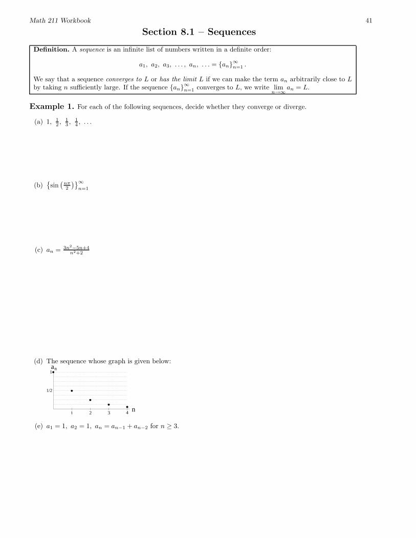
Example 1. For each of the following sequences, decide whether they converge or diverge.
(a) 1, 12 , 1
3 , 14 , . . .
(b){
sin(
nπ2
)}
∞
n=1
(c) an = 3n2−5n+4
n2+2
(d) The sequence whose graph is given below:
3
an
n
1/2
1
1 2 4
(e) a1 = 1, a2 = 1, an = an−1 + an−2 for n ≥ 3.
Math 211 Workbook 42
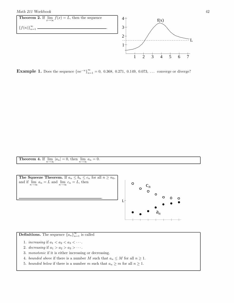
Theorem 2. If limx→∞
f(x) = L, then the sequence
{f(n)}∞n=1 .
4
L
1 2 3 4 5 6 7
f(x)
1
2
3
Example 1. Does the sequence {ne−n}∞n=1 = 0, 0.368, 0.271, 0.149, 0.073, . . . converge or diverge?
Theorem 4. If limn→∞
|an| = 0, then limn→∞
an = 0.
The Squeeze Theorem. If an ≤ bn ≤ cn for all n ≥ n0,and if lim
n→∞
an = L and limn→∞
cn = L, then
.
n
L
an
c
Definitions. The sequence {an}∞n=1 is called
1. increasing if a1 < a2 < a3 < · · · .2. decreasing if a1 > a2 > a3 > · · · .3. monotonic if it is either increasing or decreasing.
4. bounded above if there is a number M such that an ≤ M for all n ≥ 1.
5. bounded below if there is a number m such that an ≥ m for all n ≥ 1.
Math 211 Workbook 43
Theorem 6. The sequence {rn}∞n=1 is convergent if −1 < r ≤ 1 and divergent for all other values of r.
limn→∞
rn =
{
0 if −1 < r < 11 if r = 1
.
Theorem 7 (Monotonic Sequence Theorem). Every bounded, monotonic sequence is convergent.
Examples and Exercises
1. Use the Squeeze Theorem to show that the following sequences converge.
(a)
{
cosn√n
}
∞
n=1
(b)
{
3n
n!
}
∞
n=1
2. Which of the sequences from Example 1 (on the 1st page of this handout) are monotonic? bounded above?bounded below?
3. Does the sequence 0.19, 0.1919, 0.191919, . . . , converge?
Math 211 Workbook 44
Section 8.2 – Series
Preliminary Example. What is the value of the infinite sum
∞∑
n=1
1
2n?
Example 1. Let an =n
n + 1. Discuss the convergence of {an}∞n=1 and
∑
∞
n=1 an.
Math 211 Workbook 45
Example 2. Below, you are given some partial sums of the series
∞∑
n=1
1
n, which is called the harmonic series.
Does this series converge?n 10 20 30 40 50 60 70sn 2.93 3.60 3.99 4.28 4.50 4.68 4.83
Examples and Exercises
1. Each of the following is a geometric series. For each series, decide whether or not it converges, and if it does,find the sum.
(a)
∞∑
n=0
2n+1
3n(b)
∞∑
n=1
1
2·(
4
3
)n
(c) 1 − 1
3+
1
9− 1
27+
1
81− · · ·
2. For each value of an in parts (a)-(d) below, do the following.
(i) Decide whether or not the sequence {an}∞n=1 converges.
(ii) Decide whether or not the series∑
∞
n=1 an is geometric.
(iii) Decide whether or not the series∑
∞
n=1 an converges, and find the sum of the series if it is convergent.
(a) an = (−2)n−1
(b) an =n2
3n2 + 9n + 2
(c) an =3n + 2n−1
4n
(d) an =1
n(n + 1)
Math 211 Workbook 46
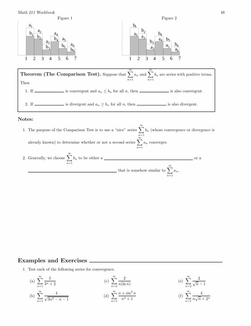
Section 8.3 – The Integral and Comparison Tests
Consider the series
∞∑
n=1
an, where an = f(n) and f is continuous, positive, and decreasing.
f(x)
4321 5 6 7
f(x)
4321 5 6 7
Theorem (The Integral Test). Suppose f is continuous, positive, and decreasing on [1,∞), and letan = f(n).
1. If diverges, then diverges.
2. If converges, then converges.
Example 1. Does
∞∑
n=1
1
2n + 3converge?
Math 211 Workbook 47
Example 2. For what values of p does the series
∞∑
n=1
1
npconverge?
Theorem (p-series test for convergence). The series
∞∑
n=1
1
npconverges if and
diverges if .
Math 211 Workbook 48
Figure 1
6
4321 5 6 7
aa
a
bb
ba
ba
bb
1
1
2
2
3
3
4
4
5a
5 6
Figure 2
b
4321 5 6 7
1
1
2
2
3
3
4
4
5
5 6
6
a
b
ab
ab
ba
ab
a
Theorem (The Comparison Test). Suppose that
∞∑
n=1
an and
∞∑
n=1
bn are series with positive terms.
Then
1. If is convergent and an ≤ bn for all n, then is also convergent.
2. If is divergent and an ≥ bn for all n, then is also divergent.
Notes:
1. The purpose of the Comparison Test is to use a “nice” series
∞∑
n=1
bn (whose convergence or divergence is
already known) to determine whether or not a second series
∞∑
n=1
an converges.
2. Generally, we choose∞∑
n=1
bn to be either a or a
that is somehow similar to
∞∑
n=1
an.
Examples and Exercises
1. Test each of the following series for convergence.
(a)
∞∑
n=1
5
3n + 2
(b)
∞∑
n=1
4√3n2 − n − 1
(c)
∞∑
n=2
2
n(lnn)
(d)
∞∑
n=1
n + sin2 n
n3 + 1
(e)
∞∑
n=2
2√n − 1
(f)
∞∑
n=1
4
n√
n + 2n
Math 211 Workbook 49
Section 8.4 – Other Convergence Tests
Preliminary Example. Let bn > 0 for all n. Consider the “alternating” series∞∑
n=1
(−1)n−1bn =
−b
0
b
b
1
2
3
4
5
b
−b
Example 1. Show that the series
∞∑
n=1
(−1)n−1
nconverges, and then estimate the value of the sum accurate to
within 0.1 of its true value.
Math 211 Workbook 50
Example 2. Which of the following series converge absolutely? Justify your answers.
(a)
∞∑
n=1
(−1)n−1
n2(b)
∞∑
n=1
(−1)n−1
n
Example 3. Use the Ratio Test to test each of the following series for convergence.
(a)
∞∑
n=1
(−1)nn2
n!(b)
∞∑
n=1
3n
n2n
Math 211 Workbook 51
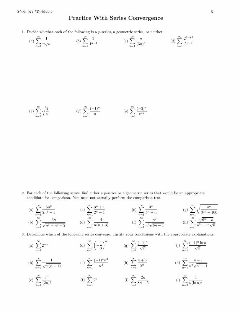
Practice With Series Convergence
1. Decide whether each of the following is a p-series, a geometric series, or neither.
(a)
∞∑
n=1
1
n√
n(b)
∞∑
n=1
3
4n−1(c)
∞∑
n=1
n
(3n)5(d)
∞∑
n=1
22n+1
5n−1
(e)
∞∑
n=1
√
2
n(f)
∞∑
n=1
(−1)n
n(g)
∞∑
n=1
(−2)n
e2n
2. For each of the following series, find either a p-series or a geometric series that would be an appropriatecandidate for comparison. You need not actually perform the comparison test.
(a)
∞∑
n=1
5n2
2n3 − 1
(b)∞∑
n=1
3n√n5 + n4 + 2
(c)
∞∑
n=1
3n + 1
2n − 1
(d)∞∑
n=1
4
n(n + 3)
(e)
∞∑
n=1
3n
5n + n
(f)∞∑
n=1
n2
n2√
6n − 1
(g)
∞∑
n=1
√
4n
32n + 100
(h)∞∑
n=1
√6n − n
42n + n√
n
3. Determine which of the following series converge. Justify your conclusions with the appropriate explanations.
(a)∞∑
n=1
2−n
(b)
∞∑
n=2
1√
n(n − 1)
(c)
∞∑
n=1
3n
(2n)!
(d)∞∑
n=1
(
−1
3
)n
(e)
∞∑
n=1
(−1)nn3
n2
(f)
∞∑
n=1
2n
(g)∞∑
n=1
(−1)n
√n
(h)
∞∑
n=1
n + 5
5n
(i)
∞∑
n=1
2n
8n − 5
(j)∞∑
n=1
(−1)n lnn√n
(k)
∞∑
n=1
n − 1
n2√
n3 + 1
(l)
∞∑
n=2
1
n(lnn)2
Math 211 Workbook 52
4. Suppose we know that 0 ≤ bn ≤ 1/n ≤ an and that 0 ≤ cn ≤ 1/n2 ≤ dn for all n.
(a) Which of the series
∞∑
n=1
an,
∞∑
n=1
bn,
∞∑
n=1
cn, and
∞∑
n=1
dn definitely converge? Justify your answer.
(b) Which of the series
∞∑
n=1
an,
∞∑
n=1
bn,
∞∑
n=1
cn, and
∞∑
n=1
dn definitely diverge? Justify your answer.
Math 211 Workbook 53
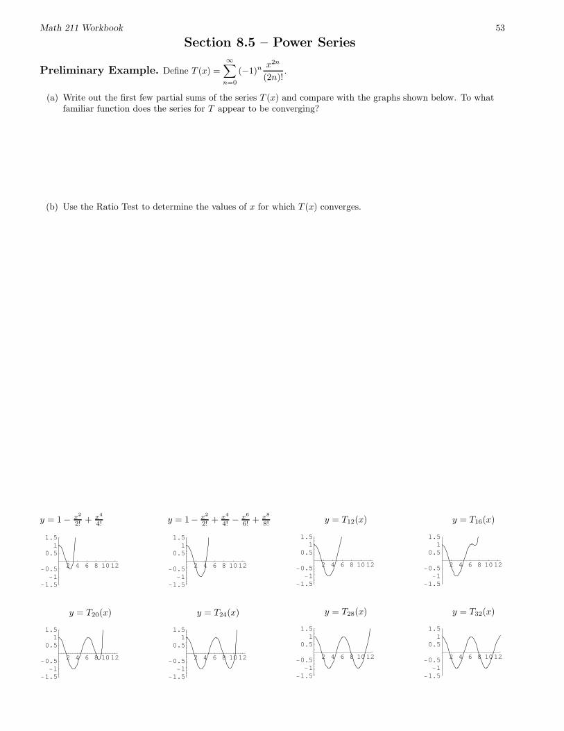
Section 8.5 – Power Series
Preliminary Example. Define T (x) =
∞∑
n=0
(−1)n x2n
(2n)!.
(a) Write out the first few partial sums of the series T (x) and compare with the graphs shown below. To whatfamiliar function does the series for T appear to be converging?
(b) Use the Ratio Test to determine the values of x for which T (x) converges.
y = 1 − x2
2! + x4
4!
2 4 6 8 1012
-1.5-1
-0.5
0.51
1.5
y = T20(x)
2 4 6 8 1012
-1.5-1
-0.5
0.51
1.5
y = 1− x2
2! + x4
4! − x6
6! + x8
8!
2 4 6 8 1012
-1.5-1
-0.5
0.51
1.5
y = T24(x)
2 4 6 8 1012
-1.5-1
-0.5
0.51
1.5
y = T12(x)
2 4 6 8 1012
-1.5-1
-0.5
0.51
1.5
y = T28(x)
2 4 6 8 1012
-1.5-1
-0.5
0.51
1.5
y = T16(x)
2 4 6 8 1012
-1.5-1
-0.5
0.51
1.5
y = T32(x)
2 4 6 8 1012
-1.5-1
-0.5
0.51
1.5
Math 211 Workbook 54
Definition. A power series is a series of the form
In this formula, x is a variable, a is a constant, and the cn’s are coefficients.
Notes:
1. We say that the above power series is centered at a. If a = 0, then the power series has the following specialform:
2. Given a power series, we seek to determine the values of the variable x for which it converges.
Example 1. Investigate the convergence of
∞∑
n=1
xn
2nat x = 0, x = 1, and x = 2.
Math 211 Workbook 55
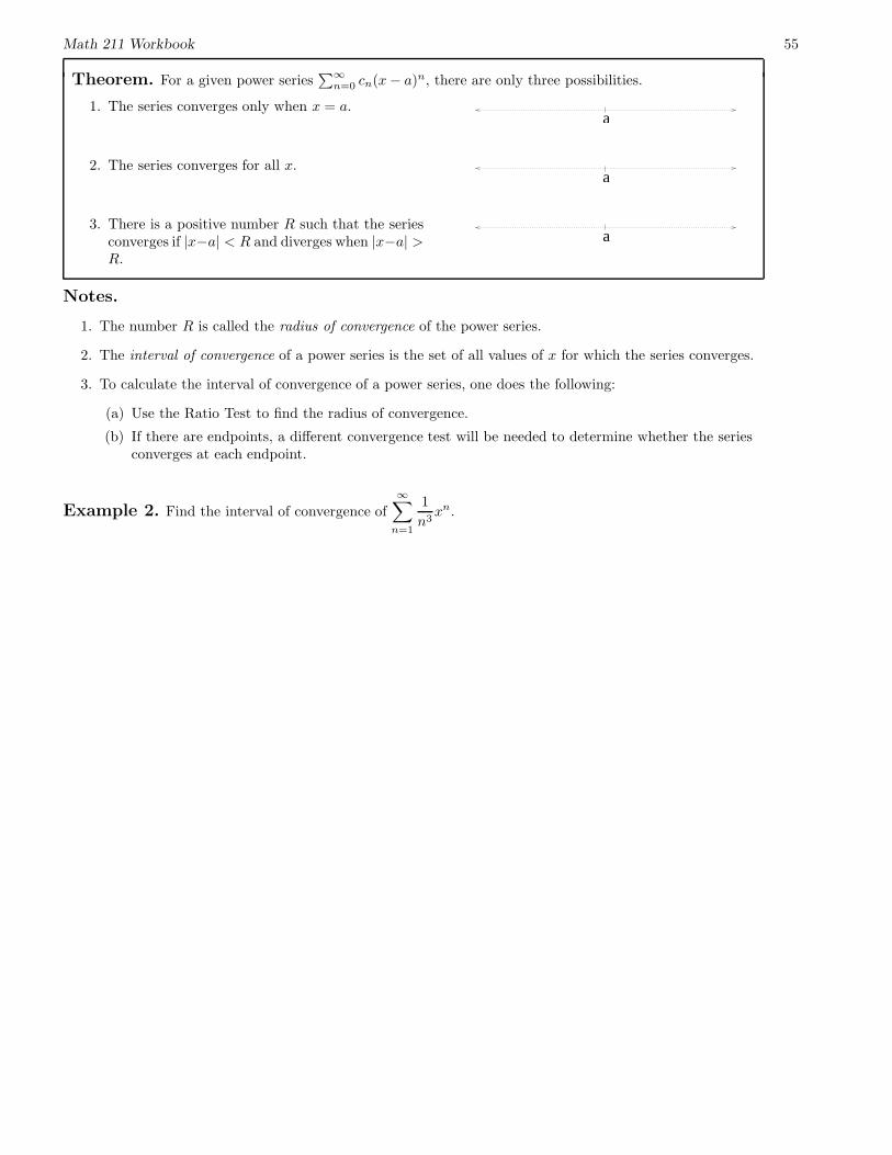
Theorem. For a given power series∑
∞
n=0 cn(x − a)n, there are only three possibilities.
1. The series converges only when x = a.a
2. The series converges for all x.a
3. There is a positive number R such that the seriesconverges if |x−a| < R and diverges when |x−a| >R.
a
Notes.
1. The number R is called the radius of convergence of the power series.
2. The interval of convergence of a power series is the set of all values of x for which the series converges.
3. To calculate the interval of convergence of a power series, one does the following:
(a) Use the Ratio Test to find the radius of convergence.
(b) If there are endpoints, a different convergence test will be needed to determine whether the seriesconverges at each endpoint.
Example 2. Find the interval of convergence of∞∑
n=1
1
n3xn.
Math 211 Workbook 56
Example 3. Find the interval of convergence of
∞∑
n=1
(2x − 3)n
√n
.
Examples and Exercises
1. Find the radius of convergence and the interval of convergence of the following power series.
(a)
∞∑
n=1
(−x)n3n
n!(b)
∞∑
n=1
n!(x − 1)n
Math 211 Workbook 57
Section 8.7 – Taylor and MacLaurin Series
Main Goal. Given a function f(x), find a power series such thatf(x) = c0 + c1(x − a) + c2(x − a)2 + c3(x − a)3 + c4(x − a)4 + · · · , where a is some real number.
Definition. Let f(x) be a function. Then the Taylor Series for f(x) centered at a is given by the formula
T (x) = f(a) +f ′(a)
1!(x − a) +
f ′′(a)
2!(x − a)2 +
f ′′′(a)
3!(x − a)3 + · · ·
=
∞∑
n=0
f (n)(a)
n!(x − a)n.
The sum of the 1st n terms of the series, Tn(x), is called the nth degree Taylor Polynomial of f(x); that is,
Tn(x) = f(a) +f ′(a)
1!(x − a) + · · · + f (n)(a)
n!(x − a)n.
Note. When the series is centered at a = 0, the Taylor series for f(x) is often called the Maclaurin series for f(x),and it has the following form:
Math 211 Workbook 58
Example 1. Build the Taylor series for f(x) = e−x centered at x = 0.
Useful Facts. Let f(x) be a function, and let
f(x) = Tn(x) + Rn(x).
1. Roughly speaking, if the remainder term Rn(x) approaches zero as n approaches infinity, then thefollowing nice things happen:
(a) The sequence T1(x), T2(x), T3(x), . . . of Taylor Polynomials converges to .This means that we can make use of the approximation
(∗) f(x) ≈ .
The closer x is to a, and the larger n is, the better the approximation will be.
(b) The Taylor Series T (x) converges to the function f(x).
2. To find the maximum possible error in the approximation (*), we look at |Rn(x)|, the absolute valueof the remainder term. It can be proven that
|Rn(x)| =
∣
∣
∣
∣
f (n+1)(z)
(n + 1)!(x − a)n+1
∣
∣
∣
∣
, where z is between a and x.
We can therefore find the maximum possible error by finding the maximum possible value of |Rn(x)|.
Math 211 Workbook 59
Example 2. Build Taylor Series for the following functions, centered at the given value of a.
(a) f(x) = sin x, a = 0 (b) g(x) = lnx, a = 1
Example 3. Use T1, T3, and T5 from Example 2 to approximate sin 1. What is the maximum possible error inyour approximation of sin 1 using T5?
Math 211 Workbook 60
Example 4. Use your Taylor series for lnx (from Example 2) to approximate ln(1.5) accurate to within 0.01 ofits true value.
Examples and Exercises
1. (a) Find the Maclaurin Series for f(x) = cosx.
(b) Use T0, T2, and T4 to find three different approximations of the value of cos(2). Use the Remainder termto find a maximum possible error for each of your approximations.
(c) Use you Maclaurin Series to estimate the value of cos(2) accurate to within 0.01 of the true value.
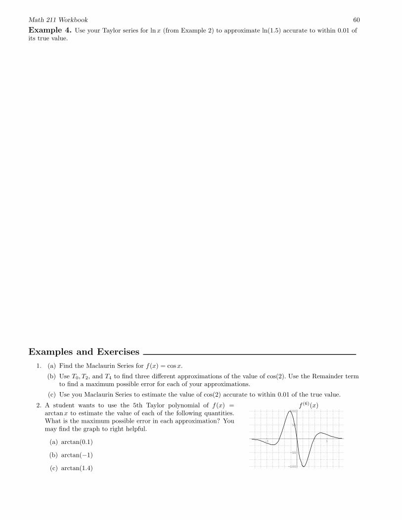
2. A student wants to use the 5th Taylor polynomial of f(x) =arctanx to estimate the value of each of the following quantities.What is the maximum possible error in each approximation? Youmay find the graph to right helpful.
(a) arctan(0.1)
(b) arctan(−1)
(c) arctan(1.4)
f (6)(x)
-1 1
-100
-50
50
100
Math 211 Workbook 61
Section 8.6 – Representation of Functions Using Power Series
Some Common Power Series
Power Series Valid For
ex = 1 + x +x2
2!+
x3
3!+
x4
4!+ · · · −∞ < x < ∞
cosx = 1 − x2
2!+
x4
4!− x6
6!+
x8
8!− · · · −∞ < x < ∞
sinx = x − x3
3!+
x5
5!− x7
7!+
x9
9!− · · · −∞ < x < ∞
1
1 − x= 1 + x + x2 + x3 + x4 + · · · −1 < x < 1
ln(1 + x) = x − x2
2+
x3
3− x4
4+
x5
5− · · · −1 < x ≤ 1
Example 1. Find a power series for f(x) = e−x2
centered at x = 0.
Example 2. Find a power series for1
1 − 5xabout x = 0. What is the radius of convergence?
Math 211 Workbook 62
Example 3. Find a power series expansion for arctanx about x = 0. What is the radius of convergence?
Examples and Exercises
1. Find a power series for each of the following (centered at x = 1 for part (c), and centered at x = 0 for allothers). What is the radius of convergence in each case?
(a)1
x − 5(b)
x
x − 5(c) ln x (d)
x
(1 − x)2
2. Use a power series to approximate
∫ 1
0
e−x2
dx to within 0.01 of its true value.
Math 211 Workbook 63
Series Overview: Some Series Definitions, Facts, and Convergence Tests
Defininition. We define the infinite series∑
∞
n=1 an to be the limit of the sequence {sn}∞n=1 of partial
sums, wheresn = a1 + a2 + a3 + · · · + an.
Therefore,
∞∑
n=1
an = limn→∞
sn =
Note. If limn→∞
sn = s, where s is a finite number, we write∑
∞
n=1 an = s, and we say that the series
to s.
Theorem (Test for Divergence).
If limn→∞
an 6= 0, then the series
∞∑
n=1
an .
Theorem (Geometric Series). Let a and r be constant. The series
a + ar + ar2 + ar3 + · · · =
∞∑
n=1
arn−1
is called a geometric series with common ratio r. We have the following facts:
1.
∞∑
n=1
arn−1 = if −1 < r < 1.
2.
∞∑
n=1
arn−1 if |r| ≥ 1.
Note:
Theorem. Suppose that∑
∞
n=1 an and∑
∞
n=1 bn converge. Then we have
1.∑
∞
n=1 (an + bn) =∑
∞
n=1 an +∑
∞
n=1 bn.
2.∑
∞
n=1 (an − bn) =∑
∞
n=1 an − ∑
∞
n=1 bn.
3. If c is constant, then∑
∞
n=1 (can) = c∑
∞
n=1 an.
Math 211 Workbook 64
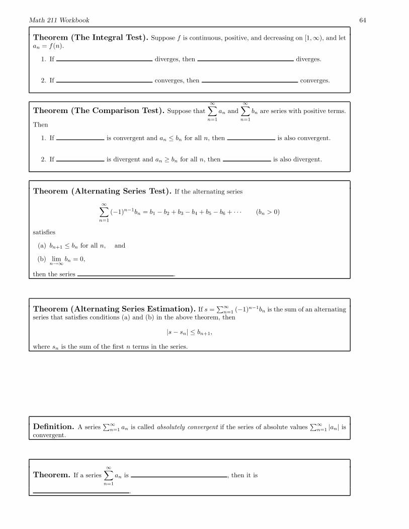
Theorem (The Integral Test). Suppose f is continuous, positive, and decreasing on [1,∞), and letan = f(n).
1. If diverges, then diverges.
2. If converges, then converges.
Theorem (The Comparison Test). Suppose that
∞∑
n=1
an and
∞∑
n=1
bn are series with positive terms.
Then
1. If is convergent and an ≤ bn for all n, then is also convergent.
2. If is divergent and an ≥ bn for all n, then is also divergent.
Theorem (Alternating Series Test). If the alternating series
n=1 (−1)n−1bn is the sum of an alternatingseries that satisfies conditions (a) and (b) in the above theorem, then
|s − sn| ≤ bn+1,
where sn is the sum of the first n terms in the series.
Definition. A series∑
∞
n=1 an is called absolutely convergent if the series of absolute values∑
∞
n=1 |an| isconvergent.
Theorem. If a series
∞∑
n=1
an is , then it is
.
Math 211 Workbook 65
Theorem (The Ratio Test).
(a) If limn→∞
∣
∣
∣
∣
an+1
an
∣
∣
∣
∣
= L < 1, then the series∞∑
n=1
an is absolutely convergent (and therefore convergent).
(b) If limn→∞
∣
∣
∣
∣
an+1
an
∣
∣
∣
∣
= L > 1, or limn→∞
∣
∣
∣
∣
an+1
an
∣
∣
∣
∣
= ∞, then the series∞∑
n=1
an diverges.
Definition. Let f(x) be a function. Then the Taylor Series for f(x) centered at a is given by the formula
T (x) = f(a) +f ′(a)
1!(x − a) +
f ′′(a)
2!(x − a)2 +
f ′′′(a)
3!(x − a)3 + · · ·
=
∞∑
n=0
f (n)(a)
n!(x − a)n.
The sum of the 1st n terms of the series, Tn(x), is called the nth degree Taylor Polynomial of f(x); that is,
Tn(x) = f(a) +f ′(a)
1!(x − a) + · · · + f (n)(a)
n!(x − a)n.
Useful Facts. Let f(x) be a function, and let
f(x) = Tn(x) + Rn(x).
1. Roughly speaking, if the remainder term Rn(x) approaches zero as n approaches infinity, then thefollowing nice things happen:
(a) The sequence T1(x), T2(x), T3(x), . . . of Taylor Polynomials converges to .This means that we can make use of the approximation
(∗) f(x) ≈ .
The closer x is to a, and the larger n is, the better the approximation will be.
(b) The Taylor Series T (x) converges to the function f(x).
2. To find the maximum possible error in the approximation (*), we look at |Rn(x)|, the absolute valueof the remainder term. It can be proven that
|Rn(x)| =
∣
∣
∣
∣
f (n+1)(z)
(n + 1)!(x − a)n+1
∣
∣
∣
∣
, where z is between a and x.
We can therefore find the maximum possible error by finding the maximum possible value of |Rn(x)|.
Math 211 Workbook 66
Section 6.4 – The Average Value of a Function
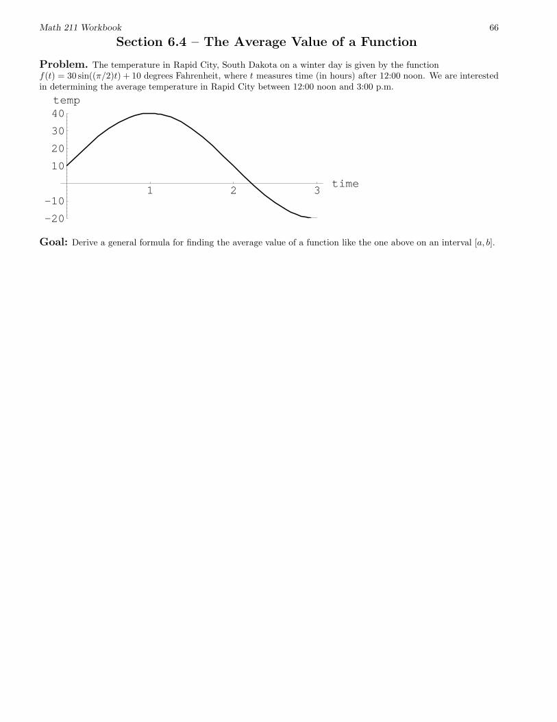
Problem. The temperature in Rapid City, South Dakota on a winter day is given by the functionf(t) = 30 sin((π/2)t) + 10 degrees Fahrenheit, where t measures time (in hours) after 12:00 noon. We are interestedin determining the average temperature in Rapid City between 12:00 noon and 3:00 p.m.
1 2 3time
-20
-10
10
20
30
40temp
Goal: Derive a general formula for finding the average value of a function like the one above on an interval [a, b].
Math 211 Workbook 67
1. Use your formula to find the average temperature in Rapid City between 12:00 noon and 3:00 p.m. on theday described on the previous page.
2. Consider the function f(x) = 4 − x2 on the interval [0, 2].
(a) Compute the average value of f(x) on [0, 2].
(b) Find c in [0, 2] such that favg = f(c).
(c) Sketch the graph of f and a rectangle whose area is the same as the area under the graph of f.
Math 211 Workbook 68
Section 6.5 – Applications to Physics and Engineering
Some Preliminary Facts:
Quantity English Unit Metric Unit
Mass
Force
Work
Example 1. What is the weight of 1 kilogram of iron?
Example 2. A 45-meter rope with a mass of 30 kg is dangling over the edge of a cliff. Ignoring friction, howmuch work is needed to pull the rope up to the top of the cliff?
(a) Explain what is wrong with the following solution to the above problem.
Work = (Force)· (Distance) = (294 N)(45 m) = 13230 Joules
Math 211 Workbook 69
(b) Give a correct solution to this problem.
Math 211 Workbook 70
Example 3. A water tank in the shape of a right circular cone of height1 meter and top radius of 0.5 meters has a column of water that has aheight of 0.5 meters. Find the work that must be done to empty the tankby pumping the water over the top edge. (Note: Water has a density of1000 kg per m3.)
0.5 m
0.5 m
1 m
Hooke’s Law. The force, f(x), needed to maintain a spring stretched x units beyond its natural lengthis proportional to x: f(x) = kx. The constant k is called the spring constant and depends on the resistanceof the spring that is being used.
of Spring
x0
Natural Length
Math 211 Workbook 71
Example 4. A spring requires a force of 50 Newtons to keep it stretched from its natural length of 15 cm to alength of 20 cm.
(a) How much force is required to keep this spring stretched to a length of 25 cm?
(b) Suppose we want to calculate the work necessary to stretch this spring from a length of 25 cm to 30 cm. Isthe solution shown below correct? Explain.
Force = 100 N
Distance = 0.05 m
Therefore,
Work = (100)(0.05) = 5 Joules.
(c) Give a correct solution to the problem posed in part (b) above.
(d) Write down a general formula for finding the work required to stretch a spring.
Math 211 Workbook 72
Exercises
1. A rope that is 20 meters long and weighs 10 Newtons per meter is hanging over the edge of a steep sea cliff sothat its bottom edge barely reaches the ground.
(a) How much work is done in pulling the rope to the top of the cliff?
(b) A surfer of mass 85 kg is stranded by high surf on a beach beneath the same cliff. How much work wouldbe required to rescue the surfer by pulling him up over the edge of the cliff (assuming that he is firmlyattached to the bottom end of the rope)?
2. (Adapted from Stewart) A circular swimming pool has a diameter of 8 meters, and the sides of the pool are 4meters high.
(a) If the pool is initially full of water, how much work is done in pumping the water out over the side? (Usethe fact that water weighs 9800 Newtons per cubic meter).
(b) If the pool is initally half full of water, how much work is done in pumping the water out over the side?
(c) Explain why your answer to part (b) is not half of your answer to part (a).
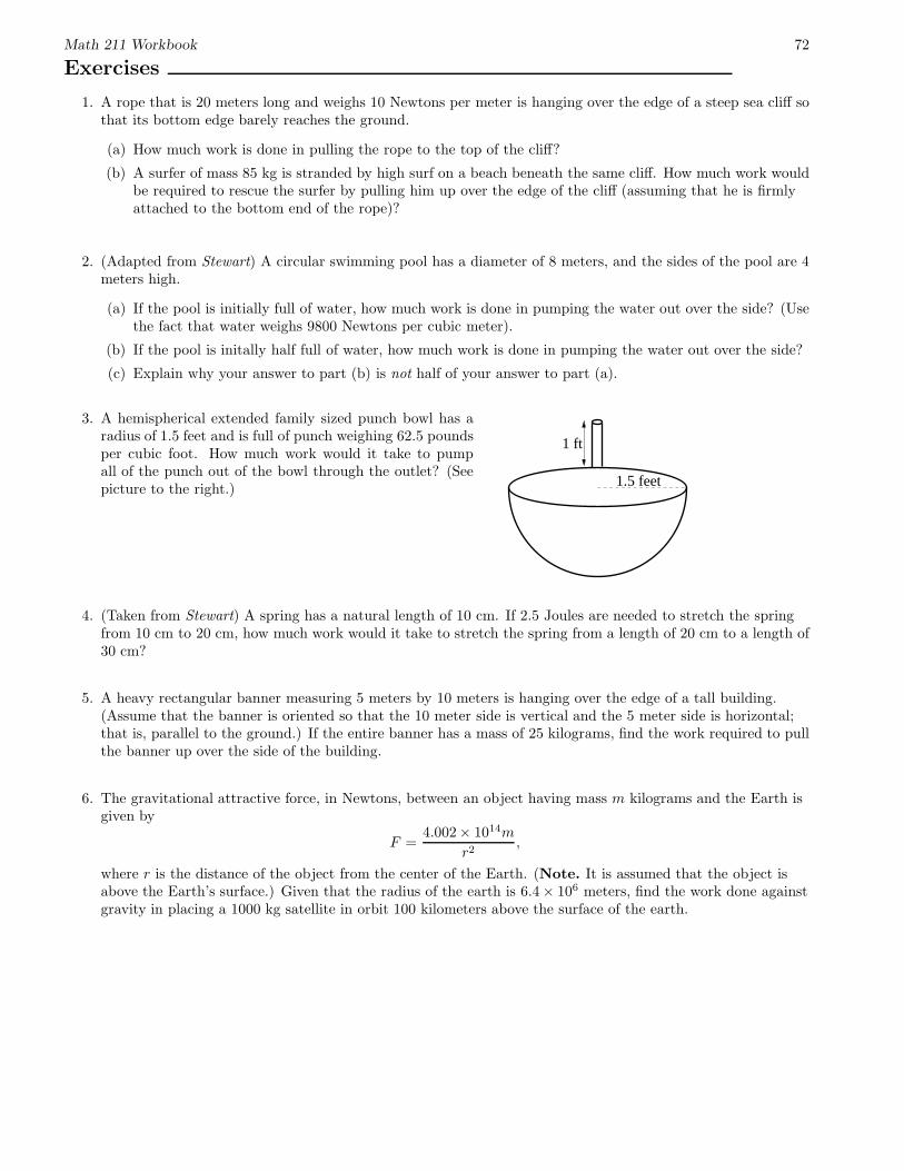
3. A hemispherical extended family sized punch bowl has aradius of 1.5 feet and is full of punch weighing 62.5 poundsper cubic foot. How much work would it take to pumpall of the punch out of the bowl through the outlet? (Seepicture to the right.)
1 ft
1.5 feet
4. (Taken from Stewart) A spring has a natural length of 10 cm. If 2.5 Joules are needed to stretch the springfrom 10 cm to 20 cm, how much work would it take to stretch the spring from a length of 20 cm to a length of30 cm?
5. A heavy rectangular banner measuring 5 meters by 10 meters is hanging over the edge of a tall building.(Assume that the banner is oriented so that the 10 meter side is vertical and the 5 meter side is horizontal;that is, parallel to the ground.) If the entire banner has a mass of 25 kilograms, find the work required to pullthe banner up over the side of the building.
6. The gravitational attractive force, in Newtons, between an object having mass m kilograms and the Earth isgiven by
F =4.002× 10¹⁴m
r2,
where r is the distance of the object from the center of the Earth. (Note. It is assumed that the object isabove the Earth’s surface.) Given that the radius of the earth is 6.4 × 10⁶ meters, find the work done againstgravity in placing a 1000 kg satellite in orbit 100 kilometers above the surface of the earth.
Math 211 Workbook 73
Functions of Two Variables: An Introduction
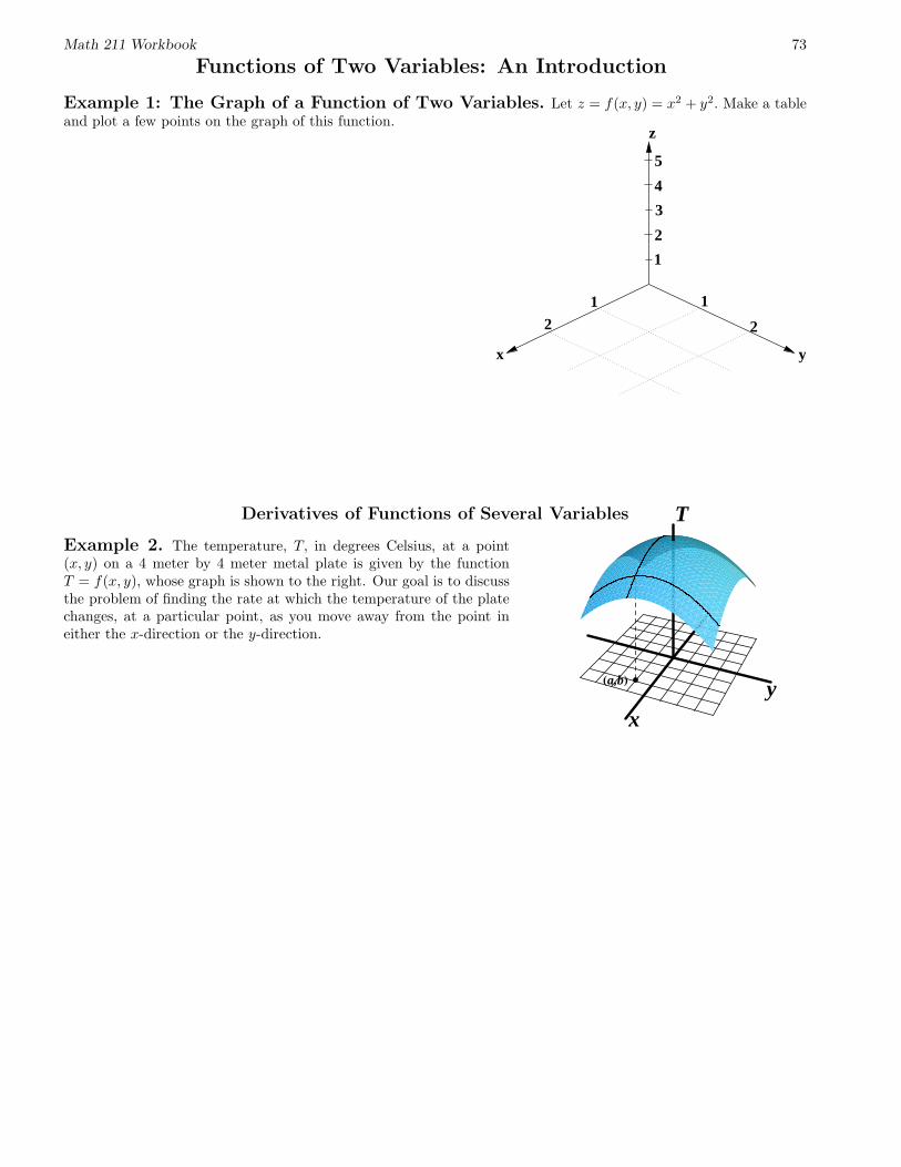
Example 1: The Graph of a Function of Two Variables. Let z = f(x, y) = x2 + y2. Make a tableand plot a few points on the graph of this function.
2
1
2
3
4
5
x
z
y
12
1
Derivatives of Functions of Several Variables
Example 2. The temperature, T, in degrees Celsius, at a point(x, y) on a 4 meter by 4 meter metal plate is given by the functionT = f(x, y), whose graph is shown to the right. Our goal is to discussthe problem of finding the rate at which the temperature of the platechanges, at a particular point, as you move away from the point ineither the x-direction or the y-direction.
Ha,bL
xy
T
Math 211 Workbook 74
Partial Derivatives of f With Respect to x and y
Let z = f(x, y). Then for all points at which the limits exist, we define the partial derivatives at thepoint (a, b) by
fx(a, b) = Rate of change of f with respect to x at (a, b) = limh→0
f(a + h, b) − f(a, b)
h,
fy(a, b) = Rate of change of f with respect to y at (a, b) = limh→0
f(a, b + h) − f(a, b)
h.
If we let a and b vary, we have the partial derivative functions fx(x, y) and fy(x, y).
Some Alternate Notations for Partial Derivatives
Again, let z = f(x, y). Then
fx =
fy =
(fx)x =
(fy)y =
(fx)y =
(fy)x =
Examples and Exercises
1. For each of the following functions, find the first partial derivatives with respect to both independentvariables.
(a) f(x, y) = yexy (b) f(x, y) =x
x2 + y2
Math 211 Workbook 75
(c) f(s, t) = sin s cos(st) (d) f(x, t) = (x + t2)4
2. For each of the following functions, find the following first and second partial derivatives: fx, fy, fxx, fyy,and fxy.
(a) f(x, y) = ex2+y2
(b) f(x, y) = x2 + xy + y2 (c) f(x, y) = x ln y
Math 211 Workbook 76
3. Given to the right is the graph of the function f(x, y) =12ye−x/2 on the domain 0 ≤ x ≤ 4 and 0 ≤ y ≤ 4.
(a) Use the graph to the right to rank the follow-ing quantities in order from smallest to largest:fx(3, 2), fx(1, 2), fy(3, 2), fy(1, 2), 0
x
y
z
(b) Use algebra to calculate the numerical values of the four derivatives from part (a) and confirm that youranswer to part (a) is correct.
Math 211 Workbook 77
Maximum and Minimum Values of Functions of Two Variables
Definitions. Let z = f(x, y) be a function of two variables.
1. We say that f(x, y) has an absolute maximum at (a, b) if f(a, b) ≥ f(x, y) for all (x, y) on the entiregraph of f.
2. We say that f(x, y) has an absolute minimum at (a, b) if f(a, b) ≤ f(x, y) for all (x, y) on the entiregraph of f.
3. We say that f(x, y) has a local maximum at (a, b) if f(a, b) ≥ f(x, y) for all (x, y) near (a, b). In thiscase, f(a, b) is called a local maximum value of f.
4. We say that f(x, y) has a local minimum at (a, b) if f(a, b) ≤ f(x, y) for all (x, y) near (a, b). In thiscase, f(a, b) is called a local minimum value of f.
5. A point (a, b) is called a critical point of f if fx(a, b) = fy(a, b) = 0.
Exercise. For each of the following functions z = f(x, y), label the points on the graph where it appears that fhas a maximum or a minimum value (indicate which type) or a critical point.
Theorem.
Question 1. At a critical point, how do we tell if we have a local maximum, a local minimum, or neither?
Math 211 Workbook 78
Theorem (Second Derivative Test). Suppose the second partial derivatives of f are continuouson a disk with center (a, b), and suppose that (a, b) is a critical point of f. (Recall that to be a “criticalpoint,” both derivatives fx and fy must equal zero at that point.) Let
D = D(a, b) = fxx(a, b)fyy(a, b) − [fxy(a, b)]2.
(a) If D > 0 and fxx(a, b) > 0, then f(a, b) is a local minimum.
(b) If D > 0 and fxx(a, b) < 0, then f(a, b) is a local maximum.
(c) If D < 0, then f(a, b) is not a local maximum or minimum.
Note 1. If D = 0, then the above test gives no information.
Note 2. If f has a critical point at (a, b) but there is no local maximum or local minimum value at (a, b), then wecall (a, b) a saddle point of f.
Question 2. How do we find the absolute maximum and minimum values of a function?
To find the absolute maximum and minimum values of a continuous function f on a closed, bounded set D:
1. Find the values of f at the of f in D.
2. Find the maximum and minimum values of f on the of D.
3. The largest of the values from steps 1 and 2 is the absolute maximum value; the smallest of thesevalues is the absolute minimum value.
Examples and Exercises1. Find all local maxima, local minima, or saddle points of for each of the following functions.
2. Find the absolute maximum and absolute minimum value of f(x, y) =x2+y2−3x−xy+3 on the closed triangular region with vertices (0, 0), (3, 0),and (3, 3) (see diagram to the right).
z
H3, 3L
H3, 0L
x
3. (Taken from Stewart) A cardboard box in the shape of a rectangular prism withouta lid is to have a volume of 32,000 cm3. Find the dimensions that minimize theamount of cardboard used. It may be helpful to follow the outline provided below.
(a) Summarize your given information by filling in the blank:
xyz = .
y
z
x
(b) Let the variable “A” represent the total surface area of the box. Write down a formula for A in terms ofthe lengths of the sides of the box. Remember that the box has no top!
(c) Using the equation from part (a) above, rewrite your formula for A so that A is a function of only x andy.
(d) Now, use the techniques of this section to minimize the function A. What should x, y, and z be so thatthe amount of cardboard used in making the box is a minimum?