Calibrating Environmental Engineering Models and Uncertainty Analysis David Ruppert Background The team The research problem The Model Environmental model Modeling the noise Likelihood Methodology Overview Locating mode Experimental Design RBF approximation MCMC sampling Case Study Chemical spill model Monte Carlo Summary and Future Research Calibrating Environmental Engineering Models and Uncertainty Analysis David Ruppert Cornell University Oct 14, 2008
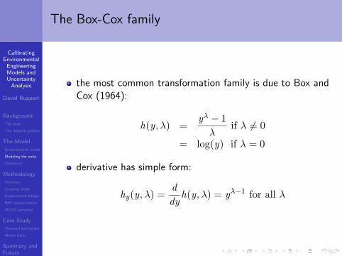
the most common transformation family is due to Box andCox (1964):
h(y, λ) =yλ − 1
λif λ 6= 0
= log(y) if λ = 0
derivative has simple form:
hy(y, λ) =ddy h(y, λ) = yλ−1 for all λ
CalibratingEnvironmental
EngineeringModels andUncertainty
Analysis
David Ruppert
BackgroundThe team
The research problem
The ModelEnvironmental model
Modeling the noise
Likelihood
MethodologyOverview
Locating mode
Experimental Design
RBF approximation
MCMC sampling
Case StudyChemical spill model
Monte Carlo
Summary andFutureResearch
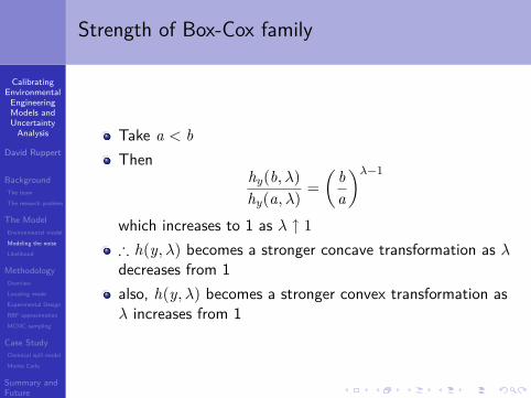
Strength of Box-Cox family
Take a < bThen
hy(b, λ)hy(a, λ)
=(
ba
)λ−1
which increases to 1 as λ ↑ 1∴ h(y, λ) becomes a stronger concave transformation as λdecreases from 1also, h(y, λ) becomes a stronger convex transformation asλ increases from 1
CalibratingEnvironmental
EngineeringModels andUncertainty
Analysis
David Ruppert
BackgroundThe team
The research problem
The ModelEnvironmental model
Modeling the noise
Likelihood
MethodologyOverview
Locating mode
Experimental Design
RBF approximation
MCMC sampling
Case StudyChemical spill model
Monte Carlo
Summary andFutureResearch
Strength of Box-Cox family, cont.
−1.0 −0.5 0.0 0.5 1.0 1.5 2.0
0.5
1.0
1.5
2.0
Example: b/a = 2
λλ
Der
ivat
ive
ratio
convex
concave
CalibratingEnvironmental
EngineeringModels andUncertainty
Analysis
David Ruppert
BackgroundThe team
The research problem
The ModelEnvironmental model
Modeling the noise
Likelihood
MethodologyOverview
Locating mode
Experimental Design
RBF approximation
MCMC sampling
Case StudyChemical spill model
Monte Carlo
Summary andFutureResearch
Technical problem with Box-Cox family
With the Box-Cox familydoes not map (0,∞) onto (−∞,∞), except for λ = 0so transformed response has a truncated normaldistributionthis makes Bayesian inference more complex
CalibratingEnvironmental
EngineeringModels andUncertainty
Analysis
David Ruppert
BackgroundThe team
The research problem
The ModelEnvironmental model
Modeling the noise
Likelihood
MethodologyOverview
Locating mode
Experimental Design
RBF approximation
MCMC sampling
Case StudyChemical spill model
Monte Carlo
Summary andFutureResearch
COIL transformation family
COnvex combination of Identity and Log (COIL) family:
hC (y, λ) = λy + (1 − λ) log(y), 0 ≤ λ ≤ 1.
We restrict λ to [0, 1), since hC (·, 1) does not map (0,∞)to (−∞,∞)COIL can approximate Box-CoxThe inverse h−1
C (·, λ) does not have a closed formevaluate by interpolation (fast)
Another family that could be used:
hC (y, λ, ε) = εy(λ) + (1 − ε) log(y)
CalibratingEnvironmental
EngineeringModels andUncertainty
Analysis
David Ruppert
BackgroundThe team
The research problem
The ModelEnvironmental model
Modeling the noise
Likelihood
MethodologyOverview
Locating mode
Experimental Design
RBF approximation
MCMC sampling
Case StudyChemical spill model
Monte Carlo
Summary andFutureResearch
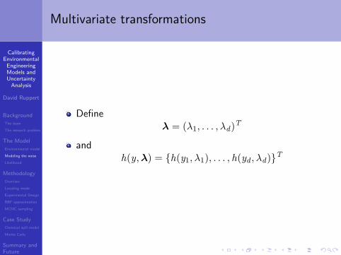
Multivariate transformations
Defineλ = (λ1, . . . , λd)T
andh(y,λ) = {h(y1, λ1), . . . , h(yd , λd)}T
CalibratingEnvironmental
EngineeringModels andUncertainty
Analysis
David Ruppert
BackgroundThe team
The research problem
The ModelEnvironmental model
Modeling the noise
Likelihood
MethodologyOverview
Locating mode
Experimental Design
RBF approximation
MCMC sampling
Case StudyChemical spill model
Monte Carlo
Summary andFutureResearch
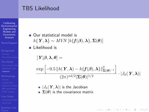
TBS Likelihood
Our statistical model ish{Y ,λ} ∼ MVN [h{f (β),λ},Σ(θ)]Likelihood is
[Y |β,λ,θ] =
exp[−0.5 ‖h(Y ,λ)− h{f (β),λ}‖2
Σ(θ)−1
](2π)nd/2|Σ(θ)|1/2 · |Jh(Y ,λ)|
|Jh(Y ,λ)| is the JacobianΣ(θ) is the covariance matrix
CalibratingEnvironmental
EngineeringModels andUncertainty
Analysis
David Ruppert
BackgroundThe team
The research problem
The ModelEnvironmental model
Modeling the noise
Likelihood
MethodologyOverview
Locating mode
Experimental Design
RBF approximation
MCMC sampling
Case StudyChemical spill model
Monte Carlo
Summary andFutureResearch
Overview of Methodology
Goal:Approximate the posterior density accurately with as fewexpensive likelihood evaluations as possible
There are four steps:1 Locate the region(s) of high posterior density2 Find an “experimental design” that covers the region of
high posterior densitythe likelihood is evaluated on this design
3 Use function evaluations from Steps 1 and 2 toapproximate the posterior
4 MCMC and standard Bayesian analysis using theapproximate posterior density
CalibratingEnvironmental
EngineeringModels andUncertainty
Analysis
David Ruppert
BackgroundThe team
The research problem
The ModelEnvironmental model
Modeling the noise
Likelihood
MethodologyOverview
Locating mode
Experimental Design
RBF approximation
MCMC sampling
Case StudyChemical spill model
Monte Carlo
Summary andFutureResearch
Removing nuisance parameters
The posterior density is
[β,λ,θ|Y ] =[β,λ,θ, Y ]∫
[β,λ,θ, Y ] dβ dλ dθ,
where [β,λ,θ, Y ] = [Y |β,λ,θ] · [β,λ,θ]
Interest focuses on
[β|Y ] =∫
[β,λ,θ|Y ] dλ dθ
CalibratingEnvironmental
EngineeringModels andUncertainty
Analysis
David Ruppert
BackgroundThe team
The research problem
The ModelEnvironmental model
Modeling the noise
Likelihood
MethodologyOverview
Locating mode
Experimental Design
RBF approximation
MCMC sampling
Case StudyChemical spill model
Monte Carlo
Summary andFutureResearch
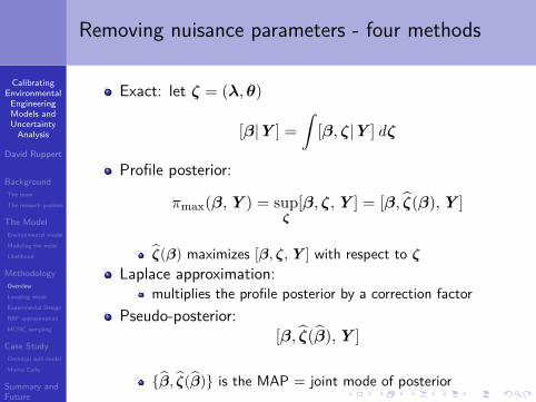
Removing nuisance parameters - four methods
Exact: let ζ = (λ,θ)
[β|Y ] =∫
[β, ζ|Y ] dζ
Profile posterior:
πmax(β, Y ) = supζ
[β, ζ, Y ] = [β, ζ(β), Y ]
ζ(β) maximizes [β, ζ, Y ] with respect to ζ
Laplace approximation:multiplies the profile posterior by a correction factor
Pseudo-posterior:[β, ζ(β), Y ]
{β, ζ(β)} is the MAP = joint mode of posterior
CalibratingEnvironmental
EngineeringModels andUncertainty
Analysis
David Ruppert
BackgroundThe team
The research problem
The ModelEnvironmental model
Modeling the noise
Likelihood
MethodologyOverview
Locating mode
Experimental Design
RBF approximation
MCMC sampling
Case StudyChemical spill model
Monte Carlo
Summary andFutureResearch
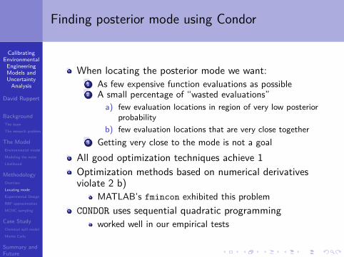
Finding posterior mode using Condor
When locating the posterior mode we want:1 As few expensive function evaluations as possible2 A small percentage of “wasted evaluations”
a) few evaluation locations in region of very low posteriorprobability
b) few evaluation locations that are very close together3 Getting very close to the mode is not a goal
All good optimization techniques achieve 1Optimization methods based on numerical derivativesviolate 2 b)
MATLAB’s fmincon exhibited this problemCONDOR uses sequential quadratic programming
worked well in our empirical tests
CalibratingEnvironmental
EngineeringModels andUncertainty
Analysis
David Ruppert
BackgroundThe team
The research problem
The ModelEnvironmental model
Modeling the noise
Likelihood
MethodologyOverview
Locating mode
Experimental Design
RBF approximation
MCMC sampling
Case StudyChemical spill model
Monte Carlo
Summary andFutureResearch
Further function evaluations needed
Goal:approximate posterior on CR(α) = {β : [β, Y ] > κ(α)}
Function evaluations in optimization stage insufficient toapproximate posterior accurately
CalibratingEnvironmental
EngineeringModels andUncertainty
Analysis
David Ruppert
BackgroundThe team
The research problem
The ModelEnvironmental model
Modeling the noise
Likelihood
MethodologyOverview
Locating mode
Experimental Design
RBF approximation
MCMC sampling
Case StudyChemical spill model
Monte Carlo
Summary andFutureResearch
Constructing the experimental design
1 Normal approximation to posteriorrequires a small number of additional function evaluations
2
CR(α) ={
β : (β − β)T[I
ββ]−1
(β − β) ≤ χ2p,1−α
}3 Space-filling design on CR(α)4 Remove points not in CR(α′) for α′ < α
E.g., α = 0.1 and α′ = 0.01
CalibratingEnvironmental
EngineeringModels andUncertainty
Analysis
David Ruppert
BackgroundThe team
The research problem
The ModelEnvironmental model
Modeling the noise
Likelihood
MethodologyOverview
Locating mode
Experimental Design
RBF approximation
MCMC sampling
Case StudyChemical spill model
Monte Carlo
Summary andFutureResearch
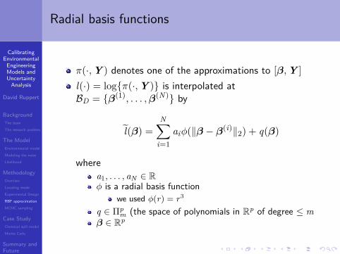
Radial basis functions
π(·, Y ) denotes one of the approximations to [β, Y ]l(·) = log{π(·, Y )} is interpolated atBD = {β(1), . . . ,β(N)} by
l(β) =N∑
i=1aiφ(‖β − β(i)‖2) + q(β)
wherea1, . . . , aN ∈ Rφ is a radial basis function
we used φ(r) = r3
q ∈ Πpm (the space of polynomials in Rp of degree ≤ m
β ∈ Rp
CalibratingEnvironmental
EngineeringModels andUncertainty
Analysis
David Ruppert
BackgroundThe team
The research problem
The ModelEnvironmental model
Modeling the noise
Likelihood
MethodologyOverview
Locating mode
Experimental Design
RBF approximation
MCMC sampling
Case StudyChemical spill model
Monte Carlo
Summary andFutureResearch
Autoregressive Metropolis-Hastings algorithm
draw MCMC sample from π(·, Y ) = exp{l(·)}restrict sample to CR(α′)
Metropolis-Hastings candidate:βc = µ + ρ(β(t) − µ) + et
et ’s are i.i.d. from density gif the candidate is accepted, then β(t+1) = βc
otherwise, β(t+1) = β(t)
CalibratingEnvironmental
EngineeringModels andUncertainty
Analysis
David Ruppert
BackgroundThe team
The research problem
The ModelEnvironmental model
Modeling the noise
Likelihood
MethodologyOverview
Locating mode
Experimental Design
RBF approximation
MCMC sampling
Case StudyChemical spill model
Monte Carlo
Summary andFutureResearch
Applications in Environmental Engineering
not enough statisticians are working on environmentalengineering problemsenvironmental engineers often use ad hoc and inefficientstatistical methodsmodern statistical techniques such as variance functions,transformations, spatial-temporal models potentially offersubstantial improvementsstatisticians and environmental engineers will both benefitfrom collaboration
CalibratingEnvironmental
EngineeringModels andUncertainty
Analysis
David Ruppert
BackgroundThe team
The research problem
The ModelEnvironmental model
Modeling the noise
Likelihood
MethodologyOverview
Locating mode
Experimental Design
RBF approximation
MCMC sampling
Case StudyChemical spill model
Monte Carlo
Summary andFutureResearch
GLUE
GLUE = Generalized Likelihood Uncertainty Estimationwidely usedconsidered state-of-the-art by many environmentalengineersreplaces the likelihood function of iid normal errors withan arbitrary objective functionshows no appreciation of maximum likelihood as a generalmethodobjective function is not based on the data-generatingprobability model
CalibratingEnvironmental
EngineeringModels andUncertainty
Analysis
David Ruppert
BackgroundThe team
The research problem
The ModelEnvironmental model
Modeling the noise
Likelihood
MethodologyOverview
Locating mode
Experimental Design
RBF approximation
MCMC sampling
Case StudyChemical spill model
Monte Carlo
Summary andFutureResearch
Synthetic data example: Chemical spill
To test algorithm:use computationally inexpensive functionthen approximate and exact result can be compared
chemical accident caused spill at two locations on a longchannel
mass M spill at location 0 at time 0mass M spill at location L and time τ
diffusion coefficient is dparameter vector is β = (m, d, l, τ)T
want estimate of average concentration at end of channell is of special interestneed assessments of uncertainty as well
CalibratingEnvironmental
EngineeringModels andUncertainty
Analysis
David Ruppert
BackgroundThe team
The research problem
The ModelEnvironmental model
Modeling the noise
Likelihood
MethodologyOverview
Locating mode
Experimental Design
RBF approximation
MCMC sampling
Case StudyChemical spill model
Monte Carlo
Summary andFutureResearch
Chemical spill model
Model is:
C(s, t; M , D, L, τ) =M
√4πDt
exp�−s2
4Dt
�
+Mp
4πD(t − τ)exp
�−(s − L)2
4D(t − τ)
�· I(τ < t)
CalibratingEnvironmental
EngineeringModels andUncertainty
Analysis
David Ruppert
BackgroundThe team
The research problem
The ModelEnvironmental model
Modeling the noise
Likelihood
MethodologyOverview
Locating mode
Experimental Design
RBF approximation
MCMC sampling
Case StudyChemical spill model
Monte Carlo
Summary andFutureResearch
Details of simulation
assume data is collected at spatial location 0 (0.5) 2.5 andtimes 0.3 (0.3) 60 (5 time 200 observations)assume that a major goal is to estimate averageconcentration of time interval [40, 140] at the end of thechannel (s = 3), specifically
F(β) =20∑
i=0f {(3, 40 + 5i),β}
requires additional function evaluations (but not muchmore computation)
CalibratingEnvironmental
EngineeringModels andUncertainty
Analysis
David Ruppert
BackgroundThe team
The research problem
The ModelEnvironmental model
Modeling the noise
Likelihood
MethodologyOverview
Locating mode
Experimental Design
RBF approximation
MCMC sampling
Case StudyChemical spill model
Monte Carlo
Summary andFutureResearch
Details, continued
λ = 0.333 in COIL familyone chemical speciesσ can be integrated out of the posterior analytically
CalibratingEnvironmental
EngineeringModels andUncertainty
Analysis
David Ruppert
BackgroundThe team
The research problem
The ModelEnvironmental model
Modeling the noise
Likelihood
MethodologyOverview
Locating mode
Experimental Design
RBF approximation
MCMC sampling
Case StudyChemical spill model
Monte Carlo
Summary andFutureResearch
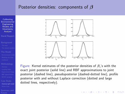
Posterior densities: components of β
9.8 10 10.2 10.40
1
2
3
4
5
β1
0.065 0.0675 0.07 0.0725 0.0750
100
200
300
400
β2
0.94 0.96 0.98 1 1.02 1.04 1.060
5
10
15
20
25
30
β3
30.1 30.12 30.14 30.16 30.18 30.20
10
20
30
40
β4
Figure: Kernel estimates of the posterior densities of βi ’s with theexact joint posterior (solid line) and RBF approximations to jointposterior (dashed line), pseudoposterior (dashed-dotted line), profileposterior with and without Laplace correction (dotted and largedotted lines, respectively).
CalibratingEnvironmental
EngineeringModels andUncertainty
Analysis
David Ruppert
BackgroundThe team
The research problem
The ModelEnvironmental model
Modeling the noise
Likelihood
MethodologyOverview
Locating mode
Experimental Design
RBF approximation
MCMC sampling
Case StudyChemical spill model
Monte Carlo
Summary andFutureResearch
Posterior densities: F(β)
124 125 126 127 128 129 130 131 132 133 1340
0.05
0.1
0.15
0.2
0.25
0.3
0.35
F(β)
Figure: Kernel smoothed density estimates for the posterior of F(β).
CalibratingEnvironmental
EngineeringModels andUncertainty
Analysis
David Ruppert
BackgroundThe team
The research problem
The ModelEnvironmental model
Modeling the noise
Likelihood
MethodologyOverview
Locating mode
Experimental Design
RBF approximation
MCMC sampling
Case StudyChemical spill model
Monte Carlo
Summary andFutureResearch
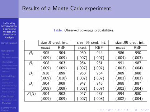
Results of a Monte Carlo experiment
MC mean ratio of C.I. lengthstrue exact RBF size .9 size .95 size .99
implemented a Bayesian method of uncertainty analysissubstantially reduced the number of evaluations of thecomputationally expensive environmental model by ameta-model based on RBF’s
CalibratingEnvironmental
EngineeringModels andUncertainty
Analysis
David Ruppert
BackgroundThe team
The research problem
The ModelEnvironmental model
Modeling the noise
Likelihood
MethodologyOverview
Locating mode
Experimental Design
RBF approximation
MCMC sampling
Case StudyChemical spill model
Monte Carlo
Summary andFutureResearch
Current and Future Work
watershed modelingCannonsville Reservoir in N.Y.
multivariate observations, e.g., several chemical speciesmultimodal posterior densitydesign: replacing local quadratic approximation by radialbasis approximation
CalibratingEnvironmental
EngineeringModels andUncertainty
Analysis
David Ruppert
BackgroundThe team
The research problem
The ModelEnvironmental model
Modeling the noise
Likelihood
MethodologyOverview
Locating mode
Experimental Design
RBF approximation
MCMC sampling
Case StudyChemical spill model
Monte Carlo
Summary andFutureResearch
Current and Future Work
automatic tuning of MCMCother transformation familiesvariance functions
as in Carroll and Ruppert, Transformations and Weightingin Regression
CalibratingEnvironmental
EngineeringModels andUncertainty
Analysis
David Ruppert
BackgroundThe team
The research problem
The ModelEnvironmental model
Modeling the noise
Likelihood
MethodologyOverview
Locating mode
Experimental Design
RBF approximation
MCMC sampling
Case StudyChemical spill model
Monte Carlo
Summary andFutureResearch
Reference
Bliznyuk, N., Ruppert, D., Shoemaker, C., Regis, R., Wild,S., and Mugunthan, P. (2008) Bayesian Calibration andUncertainty Analysis of Computationally Expensive ModelsUsing Optimization and Radial Basis FunctionApproximation, JCGS, 17, 270–294.