The IEE Measurement, Sensors, Instrumentation and NDT m Professional Network

m

Calibration of Automatic Network Analysers

Ian Instone, Agilent Technologies

0 The IEE Printed and published by the IEE, Michael Faraday House, Six Hills Way,

Stevenage, Herts SG12AY, UK

12/1

Calibration of Automatic Network Analysers

Ian Instone

Agilent Technologies UK Limited

INTRODUCTION

Network analysers are very complex instruments so it is important to define terms such as calibration to avoid confusion. The two dictionary definitions of calibration which can be applied to network analysers are “to mark (a gauge) with a scale of readings”‘, and “to correlate the readings of (an instrument etc.) with a standard”* to find the calibre o?. Unfortunately neither of these expressions defines the term calibration as it is applied to network analysers, instead they relate better to verification which is the process where the network analysers measurements are compared with those perfonned in a higher level laboratory and is described in the next paper.

DEFINITION OF CALIBRATION

Calibration in the network analyser sense is the process by which the errors within the instrument are compensated for whereas verification checks that the resultant corrections have been properly assessed and applied. The extent of calibration used will depend upon the desired measurement accuracy and the type of network analyser employed. To a large extent the available time will influence the type of calibration. There are two basic types of network analyser, both of them having their own advantages and limitations.

SCALAR NETWORK ANALYSERS

The scalar network analyser usually consists of a source, display/processor and a transducer. Earlier scalar network analysers rarely included a receiver, instead they normally employ wide band diode detectors which have the advantage of being able to make measurements over a very wide frequency range at high speed. Because this type operates over such a wide range the noise floor usually limits their low amplitude response to around -70 dBm. Diode detectors do not have a linear response to amplitude SO the displayiprocessor will also include a table of corrections (within the memory) which are applied to the measured values before being dispIayed. A very useful application of the scalar network analyser is its ability to characterise the transmission properties of mixers where the incident signal will be at a different frequency to the output signal. Filters might need to be selected to reject any unwanted signals generated by the mixer.

Figure I : Photograph oJa typical wideband detector based scalar network analyser and accessories.

More modem scalar network analysers are based on spectrum analysers (with one or more inputs) with a tracking generator (or two) included. With the rapidly decreasing costs of electronic equipment both the sources and receiver sections of these instruments are usually synthesised. A scalar network analyser of this design will be similar in complexity to it’s vector cousin, although it will lack many of the useful features (due to it being unable to measure the phase component of any signal). It will often have the advantage that it can be used as a stand-alone source or spectrum analyser, in some cases making it a more cost-effective solution.

Figure 2: Photograph of a high performance spectrum analyser based scalar network analyser which uses LI high performance external source as the tracking generator.

1212

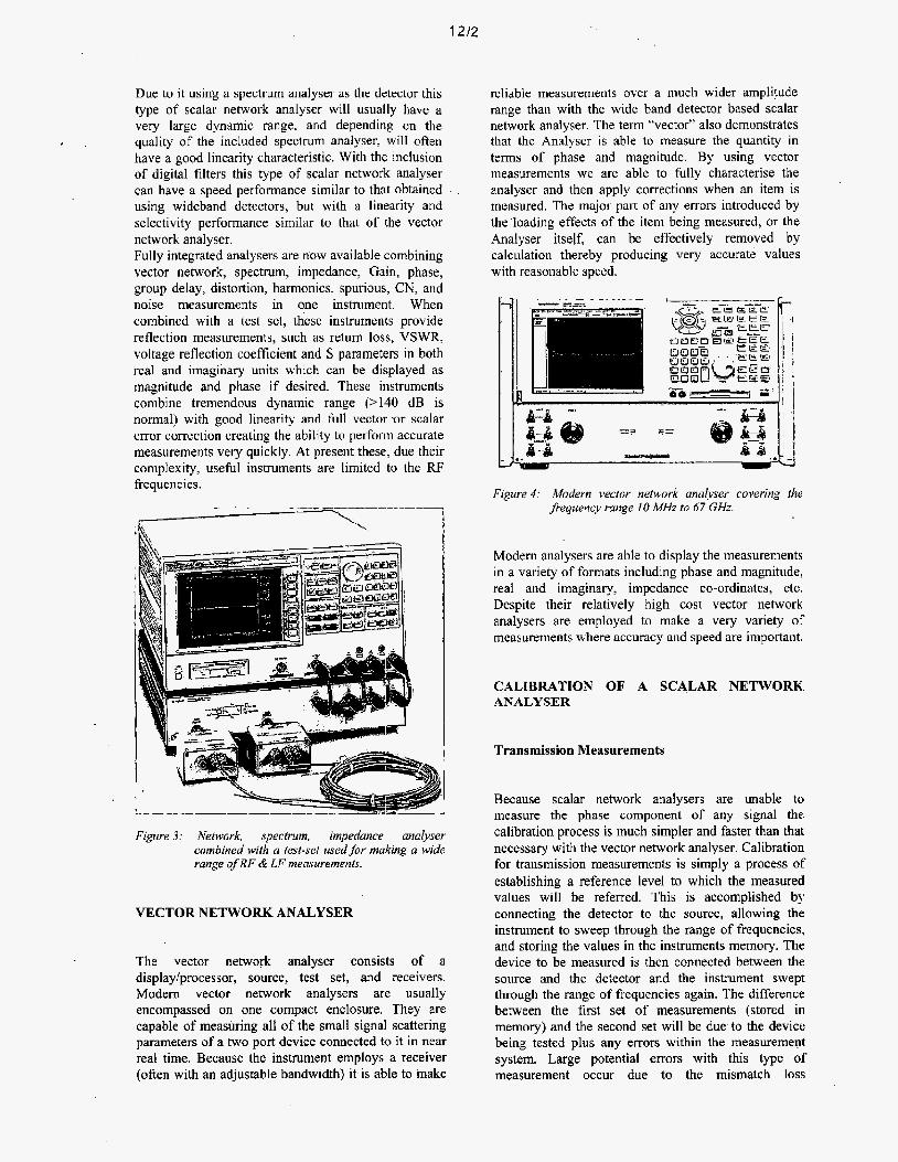
Due to it using a spectrum analyser as the detector this type of scalar network analyser will usually have a very large dynamic range, and depending on the quality of the included spectrum analyser, will often have a good linearity characteristic. With the inclusion of digital filters this type of scalar network analyser can have a speed performance similar to that obtained . using wideband detectors, but with a linearity and selectivity performance similar to that of the vector network analyser. Fully integrated analysers are now available combining vector network, spectrum, impedance, Gain, phase, group delay, distortion, harmonics. spurious, CN, and noise measurements in one instrument. When combined with a test set, these instruments provide reflection measurements, such as retum loss, VSWR, voltage reflection coefficient and S parameters in both real and imaginary units which can be displayed as magnitude and phase if desired. These instruments combine tremendous dynamic range (>140 dB is norma1) with good linearity and full vector -or scalar error correction creating the ability to perform accurate measurements very quickly. At present these, due their complexity, useful instruments are limited to the RF frequencies.

I . . - .- . - _l____l__ --

Figure 3: Nehvork, spectrum, impedance analyser combined with a test-sei used for making a wide range of RF & LF measurements.

VECTOR NETWORK ANALYSER

The vector network analyser consists of a display/processor, source, test set, and receivers. Modem vector network analysers are usually encompassed on one compact enclosure. They are capable of measuring all of the small signal scattering parameters of a two port device connected to it in near real time, Because the instrument employs a receiver (often with an adjustable bandwidth) it is able to make

reliable measurements over a much wider amplitude range than with the wide band detector based scalar network analyser. The term “vector” also demonstrates that the Analyser is able to measure the quantity in terms of phase and magnitude. By using vector measurements we are able to fully characterise the analyser and then apply corrections when an item is measured. The major part of any errors introduced by the ‘loading effects of the item being measured, or the Analyser itself, can be effectively removed by calculation thereby producing very accurate values with reasonable speed.

Figure 4: Modern vector network analyser covering the frequency range 10 MHz io 67 GHz.

Modern analysers are able to display the measurements in a variety of formats including phase and magnitude, real and imaginary, impedance co-ordinates, etc. Despite their relatively high cost vector network analysers are employed to make a very variety of measurements where accuracy and speed are important.

CALIBRATION OF A SCALAR NETWORK ANALYSER

Transmission Measurements

Because scalar network analysers are unable to measure the phase component of any signal the calibration process is much simpler and faster than that necessary with the vector network analyser. Calibration for transmission measurements is simply a process of establishing a reference level to which the measured values will be referred. This is accomplished by connecting the detector to the source, allowing the instrument to sweep through the range of frequencies, and storing the values in the instruments memory. The device to be measured is then connected between the source and the detector and the instrument swept through the range of frequencies again. The difference between the first set of measurements (stored in memory) and the second set will be due to the device being tested plus any errors within the measurement system. Large potential errors with this type of measurement occur due to the mismatch loss

12i3

uncertainties where the detector is connected to the source, and where the device being measured is connected to the source and detector. These uncertainties can be reduced by performing measurements through well matched attenuators or couplers, but it is still likely that the mismatch Ioss uncertainties will dominate the uncertainty budget. In addition, where attenuators or couplers are used their value has to be chosen very carefully. High value attenuators often have the best match and provide the best isolation against re-reflections and mismatch effects, but they also allow less of the signal to pass through, therefore reducing the effective dynamic range of the measurement, It is usually not practical to increase the source power as the higher power attenuators required to improve the match at the insertion point are often a poorer match than their lower power counterparts. Another alternative is to use a second detector and a power splitter. The ratio of the power appearing at the output ports of the power splitter is recorded (in the analysers memory) and the device to be measured connected between one output port and its’ detector. The measurements are performed again and the difference between the first and the second measurements will be due to the device being tested. Using this configuration and by connecting an appropriate attenuator between the reference detector and the power splitter, and then, perhaps by using an amplifier increasing the signal generators amplitude between the first and second measurement it is possible to make measurements using the analyser over a much wider amplitude range than it is specified. Spectrum analyser based instruments will enable a wider variety of attenuators or couplers to be used in the matching process as this type of analyser has a much wider dynamic range which copes with the additional losses much better.

Reflection Measurements

Calibrating prior to making reflection measurements follows a similar process of setting a reference and performing measurements relative to it. The input port of the bridge is connected to the generator and a short circuit connected to the bridges test port. The generator is swept through the range of desired frequencies and the values stored in the scalar network analysers memory. The short circuit is then replaced with an open circuit and the source is swept again through the range of desired frequencies and the values stored again in the analysers memory. The mean of these two sets of measurements is used as a reference and all measured values of reflection referred to it. It is important that the open circuit and short circuit are exactIy 180” apart throughout the frequency range or further errors will be present in the measurement. Because an open circuit will always have a capacitance term associated with it and a short circuit effectively shunts any capacitance it is not normally possible to satisfy this requirement over

the entire frequency range. The resultant errors are normally included as contributions to the uncertainty budget, having the most effect on the bridges source match estimate. As with transmission measurements, compromises are often made to ensure that the best quality measurement is performed without compromising speed or cost etc. For instance it is good practise to include a power splitter at the input to the bridge and connect a detector to the other output port of the power splitter. The scalar network analyser is then set to measure the ratio of the bridge over the detectors output. The power splitter and detector perform three functions:

They measure and compensate for any variations in the generators output power which may not have bqen compensated for with the generators automatic level control. When the directional bridge output port is loaded with different impedance devices connected to it (such as the short and open circuits and device being tested) it may cause the generators output amplitude to change This phenomena is almost eliminated by this arrangement. The mismatch looking into the directional bridges test port is a contribution to the measurement uncertainties, if it can be improved the uncertainties will reduce. A typical microwave generator has a fairly poor mismatch, where as power splitters have a fairly good mismatch in comparison, The mismatch of the generator or power splitter is transmitted through the bridge and will have an effect upon the resultant measurement uncertainties. When used in this configuration the effective output match of the power splitter is at its‘ best, therefore transferring the best measurement conditions through the bridge. -

Unfortunately, as with transmission measurements, there is a down side. Every power splitter has loss and inserting more loss into the measuring system will reduce the dynamic range thereby increasing the noise floor. Power splitters and detectors also cost money and each item will have a maintenance cost associated with it so including additional items in the measurements will increase costs. Inserting a good quality attenuator between the directional bridge and the source will also improve the “effective source match”. To be effective the attenuator will need to have at least 20 dB transmission loss so it will not be suitable for most wideband detector systems. This method could be the most cost effective for the spectrum analyser based system.. A reasonably high value of attenuator will perform exactly the same function as’the power splitter above but at a fraction of the cost.

1214

PROBLEMS ASSOCIATED WITH. SCALAR NETWORK ANALYSER MEASUREMENTS

The scalar network analyser . measurement system consists of a microwave generator, detector (or a bridge and detector) and a scalar network analyser. The

. scalar network analyser is very similar to an oscilloscope in construction and operation. It has an input for the x scale and several inputs for the detectors which display on the y axis. The timebase or x axis is usuaIly derived from the sweep output of the signal generator. Modem scalar network analysers also have a digital connection to the signal generator so that the display can be annotated with the start & stop frequencies, enabling easier control of the instruments. In addition the digital connection is often used to connect to printers, plotters and disk drives to provide a permanent record of the test results. It can also be used to connect a computer so that the entire measurement process, presentation and archival of results can be automated. The biggest problem with any measurement system employing diode type detectors is that they have different responses depending upon the applied power level. At low powers (< -30 dBm) they typically have a response proportional to the square of the applied power. As the power level increases their response becomes closer to a linear response. The designers of the early scalar network analysers tried to compensate for this effect by having active feedback loops in the conditioning amplifiers in the Analyser, more modem instruments compensate for these . effects digitally. Another problem is the limited dynamic range when compared to network analyser with a tuned front end. The diode detector often has a very wide frequency response (10 MHz to 26.5 GHz is common and 10 MHz to 50 MHz is becoming more popular) which results in its ability to detect and add many very small signals across its’ operating spectrum. Where each of these signals might have a very small amplitude when they are all combined they effectively produce a noise floor of around -70 dBm, At this level the random component in the measurements is usually too large for sensible measurements to be performed so scalar network analyser measurements are often limited to -60 dBm. At the higher powers the detectors might suffer from being over loaded so most diode detectors are limited to a maximum input power of about +16 d5m.

CALIBRATION OF A VECTOR NETWORK ANALYSER

The vector network analyser as the name suggests also has the capability to measure the relative phase of the signals. The measurement system employs several receivers (usually 3 or 4) to make the measurements as fast as possible without the need for extensive switching of the signals. On modern instruments the “resolution bandwidth‘.’ is switch-able allowing the

user to make compromises between accuracy and speed. A process known as “accuracy enhancement” is usually employed to reduce the errors in measurement due to the network analyser. Expressed simply, accuracy enhancement is the process whereby the network analyser is characterised using known standards so the errors within the measurement removed mathematically. Each device which is used for this characterisation is manufactured to be excellent. for only one parameter or purpose (e.g. a short should have 100 % reflection, or a load should have 100 % absorption) so it is a lot easier to manufacture these: “simple” devices than the perfect couplers which might otherwise be required. A potential confusion in terms often occurs, the term “calibration” when applied to vector network analysers is usually intended to describe the “accuracy enhancement” process. The following pages are taken from the Agilent Technologies 8722ES operating manual4 and the Hewlett-Packard HP8753A operating manual5 and describe in some detail the process of ‘‘uccuracy enhancement’’.

ACCURACY ENHANCEMENT

What Causes Measurement Errors?

Network analysis measurement errors can be separated into systematic, random, and drift errors. Correctable systematic errors are the repeatable errors that the system can measure. These are errors due to mismatch and leakage in the test setup, isolation between the reference and test signal paths, and system frequency response. The system cannot measure and correct for the non-repeatable random and drift errors. These errors affect both reflection and transmission measurements. Random errors are measurement variations due to noise and connector repeatability. Drift errors include frequency drift, temperature drift, and other physical changes in the test setup between calibration and measurement. The resulting measurement is the vector sum of the test device response plus all error terms. The precise effect of each error term depends upon its magnitude and phase relationship to the actual test device response. In most high frequency measurements the systematic errors are the most significant source of measurement uncertainty. Since each of these errors can be characterized, their effects can be effectively removed to obtain a corrected value for the test device response. For the purpose of vector accuracy enhancement, these uncertainties are quantified as directivity, source match, load match, isolation (crosstalk), and frequency response (tracking). The description of each of these systematic errors follows. Random and drift errors cannot be precisely quantified, so they must be treated as producing a cumulative uncertainly in the measured data.

Directivity

1215

Source Match

Normally a device that can separate the reverse from the forward travelling waves (a directional bridge or coupler) is used to detect the signal reflected from the test device. Ideally the coupler wouId completely separate the incident and reflected signals, and only the reflected signal would appear at the coupled output

1 1

Coupled output

r i I

Coupler Output Incident

Figure 5: Diagrammatic represen falion of an ideal directional coupler or directional bridge

However, an actual coupler is not perfect. A small amount o f the incident signal appears at the coupled output due to leakage as well as reflection from the termination in the coupled arm. Also, reflections from the coupler output connector appear at the coupled output, adding uncertainty to the signal reflected from the device.

Coupled Output

Reflected L l Figure 6: Diagrammafic represenfation of an actual

directional coupler or directional bridge showing the various error paths.

The figure of merit for how well a coupler separates forward and reverse waves is directivity. The greater the directivity of the device, the better the signal separation. System directivity is the vector sum of all leakage signals appearing at the analyzer receiver input. The error contributed by directivity is independent of the characteristics of the test device and it usually produces the major ambiguity in measurements of tow reflection devices.

Source match is defined as the vector sum of signals appearing at the analyzer receiver input due to the impedance mismatch at the test device looking back into the source, as well as to adapter and cable mismatches and losses. In a reflection measurement, the. source match error signal is caused by some of the reflected signal from the test device being reflected from the source back toward the test device and re- reflected from the test device.

hflectrd * - - -)------A

from the I Rsflsctcd source -- Incident

Figure 7: Diagrammatic representation of the constituent parts in iheformaiion of source match

In a transmission measurement, the source match error signal is caused by reflection from the test device that is re-reflected from the source. The error contributed by source match is dependent on the relationship between the actual input impedance of the test device and the equivalent match of the source. It is a factor in both transmission and reflection measurements. Source match is a particular problem in measurements .where there is a large impedance mismatch at the measurement plane. (For example, reflection devices such as filters with stop bands.)

Load Match

Load match error results from an imperfect match at the output of the test device. It is caused by impedance mismatches between the test device output port and port 2 of the measurement system. Some of the transmitted signal is reflected from port 2 back to the test device. A portion of this wave may be re-reflected to port 2, or part may be transmitted through the device in the reverse direction to appear at port 1. If the test device has low insertion loss (for example a filter pass band), the signal reflected from port 2 and re-reflected from the source causes a significant error because the test device does not attenuate the signal significantly on each reflection. The error contributed by load match is dependent on the relationship between the actual output impedance of the test device and the effective match of the retum port @ort 2). It is a factor in all transmission measurements and in reflection measurements of two-port devices.

1216

11

incidant Power (I)

R '11M = T

Reflected

CHARACTERIZING MICROWAVE SYSTEMATIC ERRORS

'11A

Figure 8: Diagrammatic representation of the constituent parts in the formation of load match.

The interaction between load match and source match is less significant when the test device insertion loss is greater than about 6 dB. However, source match and load match still interact with the input and output matches of the DUT, which contributes to transmission measurement errors. (These errors are largest for devices with highly reflective ports.)

Isolation (Crosstalk)

Leakage of energy between analyzer signal paths contributes to error in a transmission measurement, much like directivity does in a reflection measurement. Isolation is the vector sum of signals appearing at the analyzer samplers due to crosstalk between the reference and test signal paths. This includes signal leakage within the test set and in both the RF and IF sections of the receiver. The error contributed by isolation depends on the characteristics of the test device. lsolation is a factor in high-loss transmission measurements. However, analyzer system isolation is more than sufficient for most measurements, and

. correction for it may be unnecessary. For measuring devices with high dynamic range, accuracy enhancement can provide improvements in isolation that are limited only by the noise floor. Generally, the isolation falls below the noise floor, therefore, when performing an isofation calibration you should use a noise reduction function such as averaging or reduce the IF bandwidth.

Frequency Response (Tracking)

This is the vector sum of all test setup variations in which magnitude and phase change as a function of frequency. This includes variations contributed by signal-separation devices, test cables, adapters, and variations between the reference and test signal paths. This error is a factor in both transmission and reflection measurements.

One-Port Error Model

In a measurement of the reflection coefficient (magnitude and phase) of a test device, the measured data differs from the actual, no matter how carefully the measurement is made. Directivity, source match, and reflection signal path frequency response (tracking) are the major sources of error.

I I - U- mi0

Figure 9: Sources of error in rejleciion measurement.

To characterize the errors, the reflection coefficient is measured by first separating the incident signal (I) from the reflected signal (R), then taking the ratio of the two values. Ideally, (R) consists only of the signal reflected by the test device (SI IA, for SI, actual).

I 9 -

I

Figure IO: Reflection coeflcienr model.

However, all of the incident signal does not always reach the unknown. Some ,of (I) may appear at the measurement system input due to leakage through the test set or through a signal separation device. Also, some of (I) may be reflected by imperfect adapters between a signal separation device and the measurement plane. The vector sum of the leakage and the miscellaneous reflections is the effective directivity, EDF. Understandably, the measurement is distorted when the directivity signal combines with the actual reflected signal from the unknown, Si]*.

I217

I 1 Unknown

Figure I1 : Effective directiviw (EDF) model.

Since the measurement system test port is never exactly the characteristic impedance (50 ohms), some of the reflected signal bounces off the test port, or other impedance transitions further down the line, and back to the unknown, adding to the original incident signal ’ (I). This effect causes the magnitude and phase o f the incident signal to vary as a hnction of StlA and frequency. Levelling the source to produce a constant incident signal (I) reduces this error, but since the source cannot be exactly levelled at the test device input, levelling cannot eliminate all power variations. This re-reflection effect and the resultant ’incident power variation are caused by the source match error, ESF.

e

I >

R % EDF

e W Unknown

Figure 12: Source match (EsF) model.

Frequency response (tracking) error is caused by variations in magnitude and phase flatness versus frequency between the test and reference signal paths. These are due mainly to coupler roll off, imperfectly matched samplers, and differences in length and loss between the incident and test signal paths. The vector sum of these variations is the reflection signal path tracking error, ERF

Figure 13: Reflection Tracking (ERF) model.

These three errors are mathematicatly related to the actual data, SllA, and measured data, SIIM,.by the following equation:

If the value of these three “E” errors and the measured test device response were known for each frequency, this equation could be solved for S l l A to obtain the actual test device response. Because each of these errors changes with frequency, their values must be known at each test frequency. These values are found by measuring the system at the measurement plane using three independent standards whose S l l is known at all frequencies. The first standard applied is a “perfect load,” which assumes S I I = 0 and essentially measures directiviG. “Perfect load” implies a reflection-less termination at the measurement plane. All incident energy is absorbed. With S l l ~ = 0 the equation can be solved for EDF, the directivity term. In practice, of course, the “perfect load” is difficult to achieve, although very good broadband loads are available in the compatible calibration kits.

- - ~ .- .- _- Figure 14: ‘‘Pefect load” termination model.

Since the measured value for directivity is the vector sum of the actual directivity plus the actual reflection coefficient of the “perfect” load,” any reflection from the termination represents an error. System effective directivity becomes the actual reflection coefficient of the near “perfect load”.

1218

A c t u o l D i r e c t i v i t y Emfore C o r r e c t i o n

D i k e c t i v i t y A f t e r Cor r sc t Ion (nA- D, - -rL)

Meoaurad , D i r e c t i v i t y Bsfare C o r r a c t i o n (0,)

Figure 15: Vecfor diagram showing how effective directivity (EDF) is resolved.

In general, any termination having a return loss value greater than the uncorrected system directivity reduces reflection measurement uncertainty.

Figure 16: Network analyser display with a sliding load on porr 1 (S,d and a lowband load connected to porr 2 (&d.

Next, a short circuit termination whose response is known to a very high degree is used to establish another condition. The open circuit gives the third independent condition. In order to accurately model the phase variation with frequency due to fringing capacitance from the open connector, a specially designed shielded open circuit is used for this step. (The open circuit capacitance i s different with each connector type.).

(-t 1 (Em) ' l i t4 E DF + I--EsF(-I)

Figure 17: Short circuit termination model.

Now the values for EDF, directivity, ELF, source match, and ERF, reflection frequency response, are computed and stored.

lin M% 1m.0 r r i u

Figure 18: Network analyser display with short circlrits connected to both parts (SI, and S2d

T t + S l l p d f c

I

Figure 19: Open circuit terminaiion model.

This completes the calibration procedure for one port devices.

1219

Figure 20: Network analyser display with open circuiis connected to both ports ($11 and S,3.

ONE PORT DEVICE MEASUREMENT

The unknown one port device is measured to obtain values for the measured response, SLIM, at each frequency.

Figure 21: Flow diagram representing the individual constituents of an S,I reflection measurement.

This is the one port error model equation ‘solved for S1IA. Since the three errors and S l l M are now known for each test frequency, SI can be computed using the following equation:

(SI IM - Em)

E , , ( s , , M - E m ) + E , s114 =

For reflection measurements ‘on two-port devices, the same technique can be applied, but the test device output port must be terminated in the system characteristic impedance. This termination should have as low a reflection coefficient as the load used to determine directivity. The additional reflection error caused by an improper termination at the test device’s output port is not usually incorporated into the one-port error model.

TWO PORT ERROR MODEL

The error model for measurement of the transmission coefficients (magnitude and phase) of a two-port device is derived in a similar manner. The potential sources of error are frequency response (tracking), source match, load match, and isolation as shown in the figure below. On a two port network analyser these errors are effectively removed using the full two-port error model.

UFASUREMENT ERRORS

Unlrnan

Figure22: Major sources of error in transmission measurements of a two port device.

The transmission coefficient is measured by taking the ratio of the incident signal (I) and the transmitted signal (T). Refer to Figure 7-35. Ideally, (I) consists only of power delivered by the source, and (T) consists only of power emerging at the test device output.

Figure 23: Constituent parts of lhe transmission coeflcienf model.

As in the reflection model, source match can cause the incident signal to vary as a function of test device SI Also, since the test setup transmission return port is never exactly the characteristic impedance, some of the transmitted signal is reflected from the test set port 2, and from other mismatches between the test device output and the receiver input, to return to the test device. A portion of this signal may be re-reflected at port 2, thus affecting S21M, or part may be transmitted through the device in the reverse direction to appear at port 1, thus -affecting SIIM. This error term, which causes the magnitude and phase of the transmitted

12/10

signal to vary as a function of match, EL^.

is called load

W R T WRT

Figure 24: Load match error model.

The measured value, SZIM, consists of signal components that vary as a function of the relationship between ESF and SilA as well as EL^ and SZ~A, so the input and output reflection coefficients of the test device must be measured and stored for use in the error-correction computation. Thus, the test setup is calibrated as described for reflection to establish the directivity, EDF, source match, ESF, and reflection frequency response, ERF, terms for reflection measurements on both ports. Now that a calibrated port is available for reflection measurements, the thru is connected and load match, ELF, is determined by measuring the reflection coefficient of the thru connection. Transmission signal path frequency response i s then measured with the thm connected. The data is corrected for source and load match effects, then stored as transmission frequency response, ETF.

NOTE: It is very important that the exact electrical length of t h e thru be known. Most calibration kits assume a zero length thru. For some connection types such as Type-N, this implies one male and one female port. I f the test system requires a non-zero length thru, for example, one with two male test ports, the exact electrical delay of the thru adapter must be used to modify the built-in calibration kit definition of the thru.

Isolation, EXF, represents the part of the incident signal that appears at the receiver without actually passing through the test device. Isolation is measured with the test set in the transmission configuration and with terminations installed at the points where the test device will be connected. Since isolation can be lower than the noise floor, it is best to increase averaging by at least a factor of four during the isolation portion of

. the calibration.

NOTE: If the leakage (isolation) falls below the noise floor, it is best to increase averaging before calibration. If it is not possible to increase the averaging it will be better to omit the isolation measurement.

1 I I

I I

I I PORT PORT

I 2

I I

Figure 25: Isolation error model.

Thus there are two sets of error terms, forward and reverse, with each set consisting of six error terms, as follows:

k . Directivily, EDF (forward) and EDR (reverse)

> . Isolation, EXF and EXR

> . Source Match, ESF and ESR

P . Load Match, ELF and ELR

> . Transmission Tracking, ETF and ETR

R . Reflection Tracking, Ew and ERR

lin Mx3 100.0 nu,

Figure 26: Typical network anaiyser display during the isolafion mensuremenf.

Network analyser's equipped witb s-parameter test sets can measure both . the forward and reverse characteristics of the test device without you having to manually remove and physically reverse the device. A full two-port error model illustrated below. This illustration depicts how the analyzer effectively removes both the forward and reverse error terms for transmission and reflection measurements.

I 12/11

H

Figure 28: Full iwopori error model.

\

I

Figure 27: Typical network analyser displq during the “through ‘I measurement. A full two-port error model equations for all four S-

uarameters of a two-port device is shown above. Note that the mathematics for this comprehensive model [shown below) use all forward and reverse error terms and measured values. Thus, to perform full error- correction for any one parameter, all four S-parameters must be measured.

Figure 28: (below) Maihema!ical represenidion of the f i l l two port error model algoriihms.

12/12

. TRL CALIBRATION

TRL Terminology

Notice that the letters TRL, L E , LRM, etc. are often interchanged, depending on the, standards used. For

, example, "LRL" indicates that two lines and a reflect standard are used; indicates that a reflection and match standards are used. All of these refer to the same basic method. TRL* calibration is a modified form of TRL caIibration. It is adapted for a receiver with three samplers instead of four samplers. The TRL* calibration is not as accurate as the TRL calibration because it cannot isolate the source match from the load match, so it assumes load match and source match are equal.

How TRL,*ILRL* calibration works

The TRLLRL calibration used in the network analyzer relies on the characteristic impedance o f simple transmission lines rather than on a set of discrete impedance standards. Since transmission lines are relatively easy to fabricate (in a microstrip, or co-axial, for example), the impedance of these lines can be determined from the physical dimensions and substrate's dielectric constant.

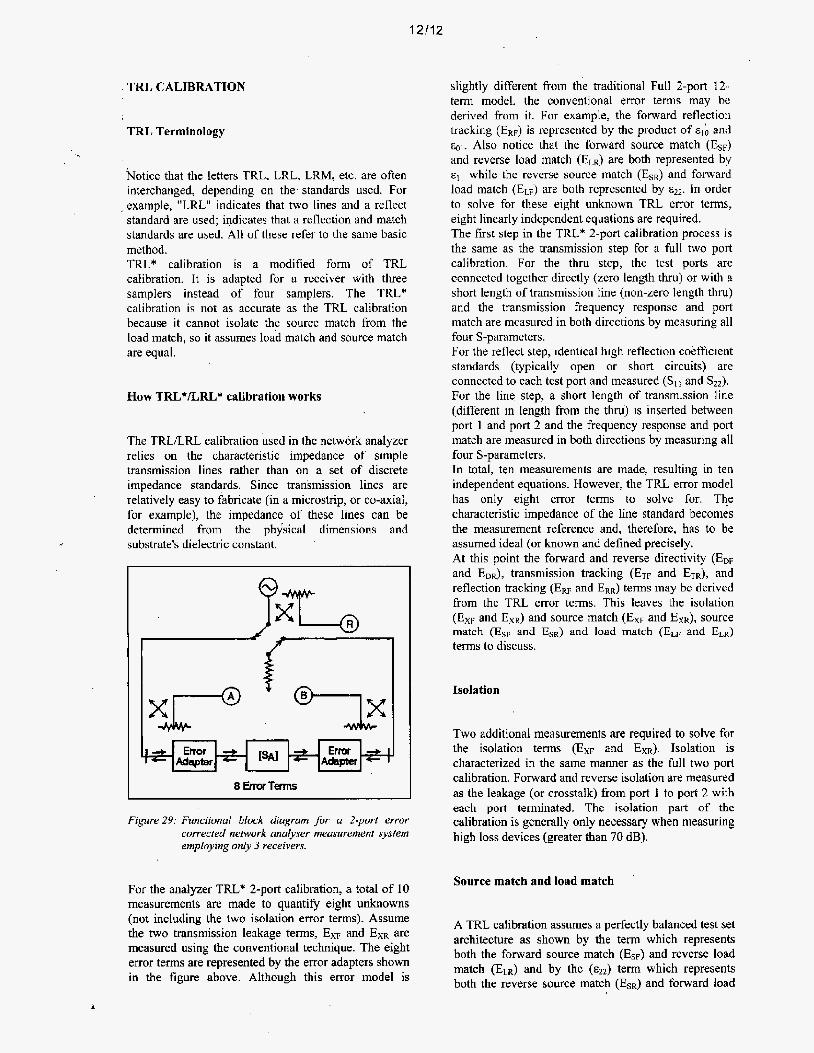
Figure29: Funcfional block diagram for a 2-port error corrected network analyser measurement system employing only 3 receivers.

For the analyzer TRL* 2-port calibration, a total of 10 measurements are made to quantify eight unknowns (not including the two isolation error terms). Assume the two transmission leakage terms, EXF and EXR are measured using the conventional technique. The eight error terms are represented by the error adapters shown in the figure above. Although this error model is

slightly different from the traditional Full 2-port 12- term model, the conventional error terms may be derived from it. For example, the forward reflection tracking (ERF) is represented by the product of E , ; and

Also notice that the forward source match (EsF) and reverse load match (ELR) are both represented by E , , while the reverse source match (ESR) and forward load match (ELF) are both represented by In order to solve for these eight unknown TRL error terms, eight linearly independent equations are required. The first step in the TRL' 2-port calibration process is the same as the transmission step for a fu l l two port calibration. For the thru step, the test ports are connected together directly (zero length thru) or with a short length of transmission line (non-zero length thru) and the transmission frequency response and port match are measured in both directions by measuring all four S-parameters. For the reflect step, identical high reflection coefficient standards (typically open or short circuits) are connected to each test port and measured (St1 and Szz). For the line step, a short length of transmission line (different in length from the thru) is inserted between port 1 and port 2 and the frequency response and port match are measured in both directions by measuring all four S-parameters. In total, ten measurements are made, resulting in ten independent equations. However, the TRL error model has only eight error terms to solve for. The characteristic impedance of the line standard becomes the measurement reference and, therefore, has to be assumed ideal (or known and defined precisely. At this point the forward and reverse directivity (EDF and EDR), transmission tracking (ETF and ETR), and reflection tracking (Ew and ERR) terms may be derived from the TRL error terms. This leaves the isolation (EXF and E X R ) and source match (EXF and EX& source match (ESF and ESR) and load match (ELF and ELR) terms to discuss.

Isolation

Two additional measurements are required to solve for the isolation terms (EXF and ExR). Isolation is characterized in the same manner as the ful l two port calibration. Forward and reverse isolation are measured as the leakage (or crosstalk) from port I to port 2 with each port terminated. The isolation part of the calibration is generally only necessary when measuring high loss devices (greater than 70 dB).

Source match and load match '

A TRL calibration assumes a perfectly balanced test set architecture as shown by the term which represents both the fonvard source match (ESF) and reverse load match (ELR) and by the (ez2) term which represents both the reverse source match (EsR) and forward load

4

12/13

match (ELF). However, in any switching test set, the source and load match terms are not equal because the transfer switch presents a different terminating impedance as it is changed between port 1 and port 2. In network analysers based on a three-sampler receiver architecture, it is not possible to differentiate the source match from the load match terms. The terminating impedance of the switch is assumed to be the same in either direction. Therefore, the test port mismatch cannot be fully corrected. An assumption is made that:

forward source match (ESF) = reverse load match (ELR) =ell

reverse source match (ESR) = forward load match (ELF) =

For a fixture, TRL* can eliminate the effects of the fixture's loss and length, but does not completely remove the effects due to the mismatch of the fixture.

NOTE: Because the technique relies on the characteristic impedance of transmission lines, the mathematically equivalent method (far line- reflect-match) may be substituted for TRL. Since a well matched termination is, in essence, an infinitely long transmission line, it is well suited far low frequency calibrations. Achieving a long line standard for low frequencies is often physically impossible.

Most of the latest network analysers are equipped with 4 receiver test-sets. In this configuration they are able to implement the full TRL algorithm.

True TRLLRL

Implementation of TRL calibration with a network analyser which employs 4 receivers requires a total of fourteen measurements to quantify ten unknowns as opposed to only a total of twelve measurements for TRL*. (Both include the two isolation error terms.) Because of the four-samplerheceiver architecture, additional correction of the source match and load match terms is achieved by measuring the ratio of the two "reference" receivers during the thru and line steps. These measurements characterize the impedance of the switch and associated hardware in both the forward and reverse measurement configurations. They are then used to modify the corresponding source and load match terms (for both forward and reverse). The four receiver configuration with TRL calibration establishes a higher performance calibration method over TRL*, because all significant error terms are systematically reduced. With TRL*, the source and load match terms are essentially that of the raw, "uncorrected" performance of the hardware where as with TRL the source and load match terms are reduced in line with the quality of calibration kit components used.

'

The TRC Calibration Procedure

When building a set of standards the following requirements satisfied:

THRU

THRU (Non Zero Length)

REFLECT

LINE/ MATCH (L"E)

LINE/ MATCH (MATCH)

for each of these standard types must be

No loss. Impedance (Z,) need not be known. s21 = SI2 = 1 L O " s,, = s 2 2 = 0

Zo of the thru must be the same as the line. Attenuation of the thru need not be known .If the thru is used to set the reference plane, the insertion phase or electrical length must be well-known and specified.

Reflection coefficient r magnitude is optimally 1 .O, but need not be known. Phase of l- must known and specified to within *!h wavelength or 90". r must be identical on both ports. If the reflect is used to set the reference plane, the phase response must be well known and specified.

Z O of the line establishes the impedance of the measurement. (i.e. Sit = S12 = 0) Insertion phase of the line must be different to the thru. Difference between Thru & line must be >20" & < 160". Attenuation need not be known. Insertion phase to be known.

Zo of the match establishes the reference impedance of the measurement. r must be identical on both ports.

When calibrating a network analyser, the actual calibration standards must have known physical characteristics. For the reflect standard, these characteristics include the offset in electrical delay (seconds) and the loss (ohmskcond of delay). The characteristic impedance, Zo is not used in the calculations in that it is determined by the line standard. The reflection coefficient magnitude should optimally be 1.0, but need not be known since the same reflection coefficient magnitude must be applied to both ports. The thru standard may be a zero-length or known length of transmission line. The value of length must be converted to electrical delay, just like that done for the reflect standard. The loss term must also be specified. The line standard must meet specific frequency related criteria, in conjunction with the length used by the thru standard. In particular, the insertion phase of the line must not be the same as the thru. The optimal line length is !A wavelength (90 degrees) relative to a zero

12/14

length thru at the frequency of interest,.and between 20 and 160 degrees of phase difference over the frequency range of interest. .(Note: these phase values can be AN x 180 degrees where N is an integer.). If two lines are used the difference in electrical length of the two lines should meet these optimal conditions. Measurement uncertainty will increase significantly

’ when the insertion phase nears zero or is an integer multiple o f 180 degrees, and this condition is not recommended. For a transmission media that exhibits linear phase over the frequency range of interest, the following expression can be used to determine a suitable line length of one-quarter wavelength at the frequency (which equals the sum of the start frequency and stop frequency divided by 2):

Electrical lenglh (em) = (Line zero iengfh THRU)

(I 5000 x V F ) Electrical length (cm) = f i ( M Z ) + f i (mz)

Where: fi = 1000 MHz & = 2000MHz VF = Velocity Factor = 1

(in this example)

Thus the length to initially check is 5 cm.

Next, use the following to verify the insertion phase at f; andf2 (1000 MBz and 2000 MHz):

(360x f X I ) Phase (deg) = V

Where: f = fiequency(MHz) 1 = length of line (cm) v = velocity

= speed of light x velocity factor

which can be reduced to the following:

0.012 x f ( M H z ) x I(“ Phase(deg rees)upprox =

VF

So for an airline (velocity factor is approximately 1) at 1000 MHz, the insertion phase is 60 degrees for a 5 cm line; it is i20 degrees at 2000 MHz. This line would be suitable as a line standard. Where the standard is fabricated in other mediums (microstrip for instance) the velocity factor is significant. For example, if the dielectric constant for a substrate is 10, and the corresponding “effective” dielectric constant for microstrip is 6.5, then the “effective” velocity factor equals 0.39 (1 + 46.5). Using the above a potential problem using TRL becomes evident. The lengths of airline required at low frequencies become so long that they are difficult to fabricate.

DATA BASED CALIBRATIONS

Traditionally the calibration standards used in any network analyser calibration routine have been defined in terms of the way in which their parameters vary in relation to the measurement frequency, for instance the open circuit would be defined in terms of capacitance. Three or four frequency terms would be employed,J; f,f and sometimesf. Open circuits would be defined in a similar manner, in terms of inductance. As correction algorithms progressed some standards were defined in terms of both capacitance and inductance. Loads were usually considered as perfect. These definitions are usually excellent providing that it is possible to define the standards using smooth curves. As processors and particularly memory have become cheaper another method of defining the calibration standards has become available, the data-based calibration. Each standard is measured across the frequency range of interest using the best equipment and techniques available. These measured values are entered into the network analyser’s database and used in .the correction algorithm’s. At frequencies where data is not available the network analyser uses interpolation, thus if measurements are made at more frequencies on the standards, the resulting network analyser measurements will become more accurate. Electronic calibration units, where the standards are in one enclosure and a switch matrix employed to apply them to the network analyser, often use a data-based calibration routine. The accuracy available from the data-based calibration employing the electronic calibration units approaches the best available from TRL calibrations, but without needing the same level of skiIled operator.

.

’ The Oxford Reference Dictionary, J.M. Hawkins, 1989 The Oxford Reference Dictionary, J.M. Hawkins, 1989 The Oxford Reference Dictionary, J.M. Hawkins, 1989 87 19ET/20ET/22ET, 87 19ES/20ES/22ES Network Analysers User’s Guide Agilent Technologies, Inc. 2000

’ HP8753A Network Analyser Operating and Programming Reference - 08753-90015 Hewlett-Packard Company. 1986 Now Agilent Technologies, Inc.