CALIBRATION OF THE SR4500 TIME-OF-FLIGHT CAMERA FOR OUTDOOR MOBILESURVEYING APPLICATIONS: A CASE STUDY

C. Heinkele∗, M. Labbe, V. Muzet, P. Charbonnier

Cerema Est, Laboratoire de Strasbourg, 11 rue Jean Mentelin, B.P. 9, 67035 Strasbourg, France{Christophe.Heinkele,Valerie.Muzet,Pierre.charbonnier}@cerema.fr, marionlabbe@free.fr

Commission V, WG V/3

KEY WORDS: SR4500, ToF Cameras, Calibration, Outdoor dynamic acquisitions

ABSTRACT:

3D-cameras based on Time-of-Flight (ToF) technology have recently raised up to a commercial level of development. In this contribu-tion, we investigate the outdoor calibration and measurement capabilities of the SR4500 ToF camera. The proposed calibration methodcombines up-to-date techniques with robust estimation. First, intrinsic camera parameters are estimated, which allows converting ra-dial distances into orthogonal ones. The latter are then calibrated using successive acquisitions of a plane at different camera positions,measured by tacheometric techniques. This distance calibration step estimates two coefficient matrices for each pixel, using linearregression. Experimental assessments carried out with a 3D laser-cloud after converting all the data in a common basis show that theobtained precision is twice better than with the constructor default calibration, with a full-frame accuracy of about 4 cm. Moreover,estimating the internal calibration in sunny and warm outdoor conditions yields almost the same coefficients as indoors. Finally, a testshows the feasibility of dynamic outdoor acquisitions and measurements.

1. INTRODUCTION

In this contribution, we study the metrological performance (setupand calibration) and the measurement capacities of a recent Time-of-Flight (ToF) camera, namely the SR4500, in the context ofoutdoor mobile surveying applications.

Range cameras have become considerably popular in the last de-cades, thanks to their ability to simultaneously acquire a rangemap and an intensity matrix, at a low cost and video frame rate.Thanks to the progress of technologies, they have raised up toa commercial level of development and are now routinely usedin many applications, such as robotics, medicine, automobile orvideo gaming. Nowadays, industrial 3D cameras offer a cheap al-ternative, albeit less accurate, to laser scanners for short-range 3Dsurveying in controlled environments. However, the recent appli-cation of range cameras to outdoor 3D surveying at longer ranges(Chiabrando and Rinaudo, 2013, Lachat et al., 2015) raises thequestion of their metrological capabilities.

Range cameras based on ToF technologies have recently encoun-tered an increasing attention, see e.g. (Piatti et al., 2013). Sev-eral industrial sensors were developed since the seminal work of(Lange, 2000), see e.g. (Piatti and Rinaudo, 2012) for a survey.In this contribution, we consider a phase modulated (or indirectToF) camera, namely the SR4500 (Fig. 1), launched in 2014 andmanufactured by Mesa Imaging (recently acquired by the Hep-tagon company). The sensor operates in the close infrared. It isan in-pixel photomixing device (Pancheri and Stoppa, 2013), i.e.it operates a demodulation of the received optical signal for eachpixel.

While the former versions of the camera were limited to 5 meters,the SR4500 has the advantage of measuring up to 10 m, depend-ing on the acquisition frequency (frequencies may be set between15 and 30 MHz). The integration time may be set in the range[0.3-25.8] ms. Its resolution is 176×144 pixels, for a field of

∗Corresponding author

Figure 1. Picture of the SR4500 ToF camera

view of 69◦×55◦. A sample acquisition is shown on Fig. 2. Thescene is taken in a technical hall, with an optical bench and a testvehicle. Its depth varies from 0 to 10 m. The left image showsthe depth map (in false colors), where the depth gradient alongthe bench is clearly visible, along with some noisy pixels. Thecenter image is the intensity image in the infrared which is, ofcourse, slightly different from the rightmost photograph.

(a) (b) (c)

Figure 2. Sample acquisition of an indoor scene by the SR4500ToF camera. (a) Distance matrix (b) amplitude matrix, in theclose infrared (c) Photograph of the scene taken by an externalcamera

We have chosen the SR4500 camera because it is well suited toour research activity, that aims at developing tools for outdoor

The International Archives of the Photogrammetry, Remote Sensing and Spatial Information Sciences, Volume XLI-B5, 2016 XXIII ISPRS Congress, 12–19 July 2016, Prague, Czech Republic

This contribution has been peer-reviewed. doi:10.5194/isprsarchives-XLI-B5-469-2016

469

mobile surveying applications. More specifically, we want to sur-vey objects (e.g. traffic signs) in urban road scenes, at a [3-8] mdistance range, using dynamic acquisitions. In such a context,short integration times (typically less than 10 ms) are required,at the price of more noisy acquisitions, which implies applyingrobust data processing methods.

In this paper, we first propose an introduction to the SR4500 cam-era and its behaviour (Sec. 2). It is clear that raw measurementsare not accurate enough so a calibration is needed. In the lit-erature, several publications report works on the calibration andmetrological assessment of ToF cameras (in particular, of previ-ous versions of SR cameras), see e.g. (Kahlmann et al., 2006,Jaakkola et al., 2008, Robbins et al., 2008, Chiabrando et al.,2009, Lefloch et al., 2013). Inspired by these papers, we intro-duce in Sec. 3 a two-step calibration methodology. Sec. 4 is dedi-cated to an experimental assessment of this method in laboratoryand outdoor conditions. Finally, Sec. 5 is a feasibility study ofdynamic outdoor acquisitions and measurements.

2. BEHAVIOUR OF THE SR4500 CAMERA

2.1 Measurement principle

The SR4500 processes each pixel using the continuous wave in-tensity modulation method, which is based on the correlation be-tween the emitted signal and the received one (Lange, 2000). Theemitted light being sinusoidal, with a fixed frequency f , the cor-relation function can be written, at τ = 2πft, as (Lefloch et al.,2013):

cτ = A0 +A

2cos(τ + ϕ) (1)

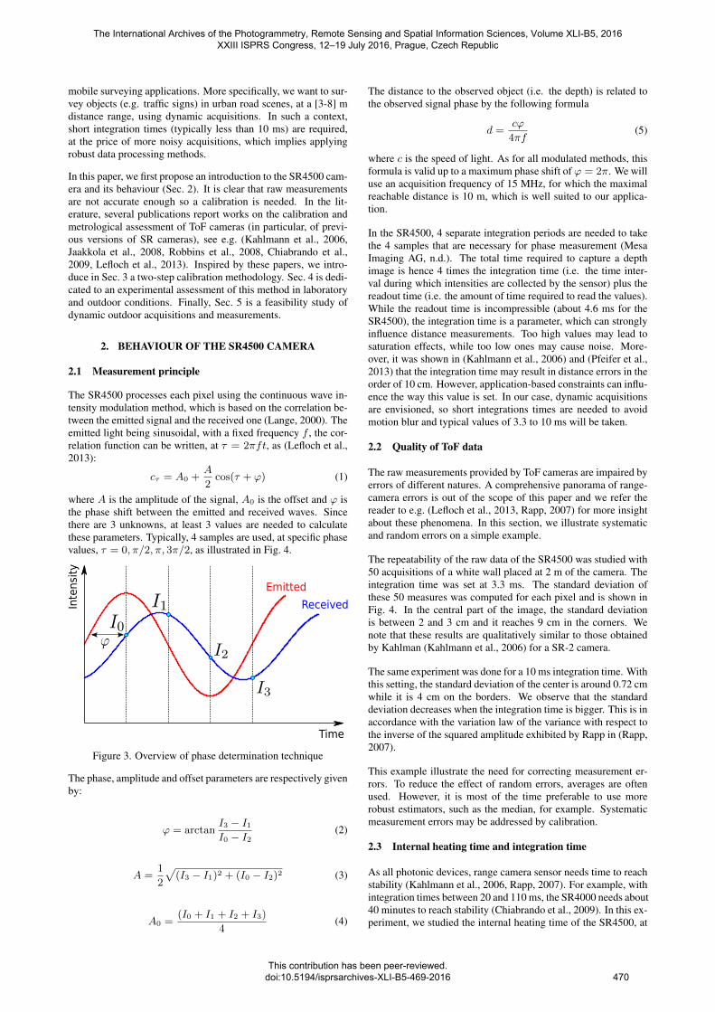
where A is the amplitude of the signal, A0 is the offset and ϕ isthe phase shift between the emitted and received waves. Sincethere are 3 unknowns, at least 3 values are needed to calculatethese parameters. Typically, 4 samples are used, at specific phasevalues, τ = 0, π/2, π, 3π/2, as illustrated in Fig. 4.

Emitted

Time

Intensity

Received

Figure 3. Overview of phase determination technique

The phase, amplitude and offset parameters are respectively givenby:

ϕ = arctanI3 − I1I0 − I2

(2)

A =1

2

√(I3 − I1)2 + (I0 − I2)2 (3)

A0 =(I0 + I1 + I2 + I3)

4(4)

The distance to the observed object (i.e. the depth) is related tothe observed signal phase by the following formula

d =cϕ

4πf(5)

where c is the speed of light. As for all modulated methods, thisformula is valid up to a maximum phase shift of ϕ = 2π. We willuse an acquisition frequency of 15 MHz, for which the maximalreachable distance is 10 m, which is well suited to our applica-tion.

In the SR4500, 4 separate integration periods are needed to takethe 4 samples that are necessary for phase measurement (MesaImaging AG, n.d.). The total time required to capture a depthimage is hence 4 times the integration time (i.e. the time inter-val during which intensities are collected by the sensor) plus thereadout time (i.e. the amount of time required to read the values).While the readout time is incompressible (about 4.6 ms for theSR4500), the integration time is a parameter, which can stronglyinfluence distance measurements. Too high values may lead tosaturation effects, while too low ones may cause noise. More-over, it was shown in (Kahlmann et al., 2006) and (Pfeifer et al.,2013) that the integration time may result in distance errors in theorder of 10 cm. However, application-based constraints can influ-ence the way this value is set. In our case, dynamic acquisitionsare envisioned, so short integrations times are needed to avoidmotion blur and typical values of 3.3 to 10 ms will be taken.

2.2 Quality of ToF data

The raw measurements provided by ToF cameras are impaired byerrors of different natures. A comprehensive panorama of range-camera errors is out of the scope of this paper and we refer thereader to e.g. (Lefloch et al., 2013, Rapp, 2007) for more insightabout these phenomena. In this section, we illustrate systematicand random errors on a simple example.

The repeatability of the raw data of the SR4500 was studied with50 acquisitions of a white wall placed at 2 m of the camera. Theintegration time was set at 3.3 ms. The standard deviation ofthese 50 measures was computed for each pixel and is shown inFig. 4. In the central part of the image, the standard deviationis between 2 and 3 cm and it reaches 9 cm in the corners. Wenote that these results are qualitatively similar to those obtainedby Kahlman (Kahlmann et al., 2006) for a SR-2 camera.

The same experiment was done for a 10 ms integration time. Withthis setting, the standard deviation of the center is around 0.72 cmwhile it is 4 cm on the borders. We observe that the standarddeviation decreases when the integration time is bigger. This is inaccordance with the variation law of the variance with respect tothe inverse of the squared amplitude exhibited by Rapp in (Rapp,2007).

This example illustrate the need for correcting measurement er-rors. To reduce the effect of random errors, averages are oftenused. However, it is most of the time preferable to use morerobust estimators, such as the median, for example. Systematicmeasurement errors may be addressed by calibration.

2.3 Internal heating time and integration time

As all photonic devices, range camera sensor needs time to reachstability (Kahlmann et al., 2006, Rapp, 2007). For example, withintegration times between 20 and 110 ms, the SR4000 needs about40 minutes to reach stability (Chiabrando et al., 2009). In this ex-periment, we studied the internal heating time of the SR4500, at

The International Archives of the Photogrammetry, Remote Sensing and Spatial Information Sciences, Volume XLI-B5, 2016 XXIII ISPRS Congress, 12–19 July 2016, Prague, Czech Republic

This contribution has been peer-reviewed. doi:10.5194/isprsarchives-XLI-B5-469-2016

470

Figure 4. Standard deviation (m) of 50 acquisitions (sight dis-tance of 2 m, integration time of 3.3 ms)

20 40 60 80

3.2

3.3

3.4

3.5

Time (min)

Mea

sure

ddi

stan

ce(m

)

3.3 ms5.3 ms10 ms20 ms

Real distance

20 40 60 80

1.5

2

2.5

3·10−2

Time (min)

Stan

dard

devi

atio

n(m

)

Figure 5. Evolution of the measured distance (left) and standarddeviation (right) with time for different acquisition times

a sight distance of 3.5 m for 4 different integration time: 3.3, 5.3,10 and 20 ms. For each integration time, 50 acquisitions weretaken every 5 min and we studied the raw data given by the Mesasoftware. The median and the standard deviation are presentedfor the central part of the image (30×24 pixels) in Fig. 5. Themeasured distance almost corresponds to the real distance at 3.3and 5.5 ms while there is an important distance offset at 10 and20 ms. Since the default value of the Mesa SR4500 integrationtime is 3.3 ms (Mesa Imaging AG, n.d.), it seems that the defaultcalibration corresponds to this setting. For the longest integrationtimes of our study (10 and 20 ms), during the first 20 minutes ofheating, the variation of the measured distance reaches 4 cm. Atan acquisition time of 3.3 ms, there is less variation of the mediandistance but the standard deviation needs more time to reach sta-bility (40 to 60 minutes). Hence, a heating time of 40 min at leastwas systematically respected in all our experiments.

This experiment confirms the need for a correction of distances.Clearly, this calibration must be adapted to each integration timesetting.

3. CALIBRATION METHODOLOGY

Sources of systematic error are many in range imaging, see e.g.(Lefloch et al., 2013). In such a context, substantial gains in pre-cision are accessible using calibration techniques. In this section,

Figure 6. Transforming a radial distance into an orthogonal dis-tance, following (Rapp et al., 2008)

Figure 7. Photographs of the calibration checkerboard installedindoors (a) and outdoors (c); corresponding amplitude imagesoutput by the SR4500 indoors (b) and outdoors(d)

we recall the basis ideas of the two calibration procedures we use.The first one, internal, or lateral (Lindner and Kolb, 2006), cali-bration aims at transforming the radial distance provided by therange camera into an orthogonal distance, or depth. The secondone, distance or depth calibration, is used to adjust the outputs toreference measurements.

3.1 Internal calibration

As for ordinary cameras, the internal calibration of range cam-eras relies on the determination of the intrinsic parameters of thedevice. These camera-specific parameters are, in particular, thefocal length f , the optical image center (cx, cy), the pixel sizeand the distortion coefficients. Once these parameters are esti-mated, it is possible to compensate for distortions caused by thesensor lens, but also to convert any radial distance Drad into anorthogonal oneDorth using the pin-hole model, as described e.g.in (Rapp et al., 2008), see Fig. 6. The transformation is governedby the following relationship:

Dorth = Drad. cos

(arctan

(√x2p + y2pf

))(6)

where (xp, yp) are the coordinate of the point in the image plane.

Among the multiple available calibration packages, we have cho-sen Bouguet’s Matlabr calibration toolbox (Bouguet, 1999). Sev-eral views of a specially designed calibration checkerboard (seeFig. 7), whose dimensions (3×2.4 m) are well suited to our ap-plication, are taken. More specifically, the corresponding ampli-tude matrices provided by the SR4500 are used as data inputs.In practice we do not use all the parameters output by Bouguet’s

The International Archives of the Photogrammetry, Remote Sensing and Spatial Information Sciences, Volume XLI-B5, 2016 XXIII ISPRS Congress, 12–19 July 2016, Prague, Czech Republic

This contribution has been peer-reviewed. doi:10.5194/isprsarchives-XLI-B5-469-2016

471

calibration routine. For example, we found that the focal distancewas almost the same along both axes, and that the skew angleand tangential distortion coefficients could be neglected. More-over, we consider a fourth-order radial distortion model, due tothe negligible influence of the sixth order.

3.2 Distance calibration

The second step consists of the calibration of the orthogonal dis-tances obtained from eq. (6). Successive images of a plane sur-face are taken with the SR4500 at different distances, as illus-trated on Fig. 8. These reference distances are measured with avery accurate system (such as laser scanners, tacheometers (Chiabrandoet al., 2009) or linear positionner tables (Rapp, 2007)).

Figure 8. Scheme of the distance calibration method: referencedistances are drawn in blue and SR4500 outputs are in red

In this work, we perform a per-pixel linear calibration. In otherwords, a linear regression is computed for each pixel, to adjustthe data given by the camera to the reference distances. The out-put of the procedure is hence a pair of 25344-element matrices:one for the slopes and one for the offsets. Other techniques mightbe used, such as lookup tables (Kahlmann et al., 2006), but lin-ear adjustment is more storage-efficient, as noticed in (Lindnerand Kolb, 2006). While more sophisticated models, involving B-spline global correction (Lindner and Kolb, 2006) or polynomialregression (Schiller et al., 2008), might be envisioned, we foundthat the linear model was a good compromise between accuracyand complexity for our applications.

4. EXPERIMENTAL CALIBRATIONS

In this section, we propose an experimental assessment of thecalibration methodology in both indoor and outdoor conditions.

4.1 Internal calibration

The calibration checkerboard has been used indoors and outdoors.In the indoor setting it is fixed on a wall and the camera is placedon a tripod; outdoors, it is laid on the floor and the SR4500 isattached to a forklift as depicted on Fig. 9. Figure 10 shows theposition and orientation of the views taken in both situations.

Table 1 shows a comparison of the intrinsic parameters obtainedin both configurations. Although the uncertainties provided byBouguet’s toolbox significatively increased outdoors, the differ-ences of the computed parameters are quite small.

Despite the experimental conditions were not perfect (in partic-ular, the ground is not really plane), this experiment shows thefeasibility of an internal calibration outdoors, which might be ofa great interest for future applications.

Figure 9. The SR4500 is fixed on a forklift for outdoor internalcalibration

Figure 10. Orientation of the camera during indoor calibration(top) and outdoor calibration (bottom)

Indoor calibration Outdoor calibrationvalues uncertainties values uncertainties

fx 10.09 0.09 10.08 0.18fy 10.09 0.08 10.08 0.19cx 3.61 0.12 3.62 0.11cy 2.65 0.11 2.72 0.17

Table 1. Comparison of the SR4500 intrinsic parameters in mmbetween indoor and outdoor calibration

The International Archives of the Photogrammetry, Remote Sensing and Spatial Information Sciences, Volume XLI-B5, 2016 XXIII ISPRS Congress, 12–19 July 2016, Prague, Czech Republic

This contribution has been peer-reviewed. doi:10.5194/isprsarchives-XLI-B5-469-2016

472

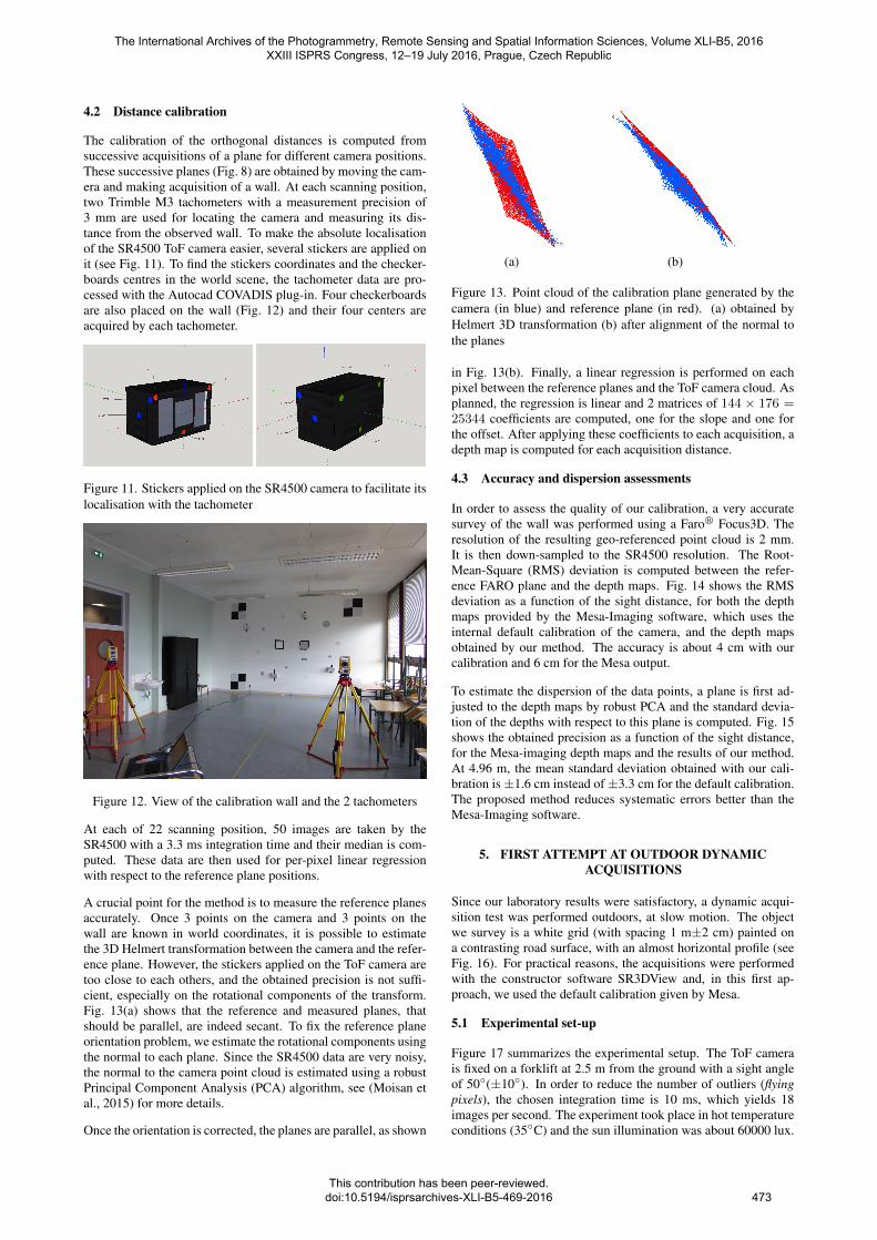
4.2 Distance calibration

The calibration of the orthogonal distances is computed fromsuccessive acquisitions of a plane for different camera positions.These successive planes (Fig. 8) are obtained by moving the cam-era and making acquisition of a wall. At each scanning position,two Trimble M3 tachometers with a measurement precision of3 mm are used for locating the camera and measuring its dis-tance from the observed wall. To make the absolute localisationof the SR4500 ToF camera easier, several stickers are applied onit (see Fig. 11). To find the stickers coordinates and the checker-boards centres in the world scene, the tachometer data are pro-cessed with the Autocad COVADIS plug-in. Four checkerboardsare also placed on the wall (Fig. 12) and their four centers areacquired by each tachometer.

Figure 11. Stickers applied on the SR4500 camera to facilitate itslocalisation with the tachometer

Figure 12. View of the calibration wall and the 2 tachometers

At each of 22 scanning position, 50 images are taken by theSR4500 with a 3.3 ms integration time and their median is com-puted. These data are then used for per-pixel linear regressionwith respect to the reference plane positions.

A crucial point for the method is to measure the reference planesaccurately. Once 3 points on the camera and 3 points on thewall are known in world coordinates, it is possible to estimatethe 3D Helmert transformation between the camera and the refer-ence plane. However, the stickers applied on the ToF camera aretoo close to each others, and the obtained precision is not suffi-cient, especially on the rotational components of the transform.Fig. 13(a) shows that the reference and measured planes, thatshould be parallel, are indeed secant. To fix the reference planeorientation problem, we estimate the rotational components usingthe normal to each plane. Since the SR4500 data are very noisy,the normal to the camera point cloud is estimated using a robustPrincipal Component Analysis (PCA) algorithm, see (Moisan etal., 2015) for more details.

Once the orientation is corrected, the planes are parallel, as shown

(a) (b)

Figure 13. Point cloud of the calibration plane generated by thecamera (in blue) and reference plane (in red). (a) obtained byHelmert 3D transformation (b) after alignment of the normal tothe planes

in Fig. 13(b). Finally, a linear regression is performed on eachpixel between the reference planes and the ToF camera cloud. Asplanned, the regression is linear and 2 matrices of 144 × 176 =25344 coefficients are computed, one for the slope and one forthe offset. After applying these coefficients to each acquisition, adepth map is computed for each acquisition distance.

4.3 Accuracy and dispersion assessments

In order to assess the quality of our calibration, a very accuratesurvey of the wall was performed using a Faror Focus3D. Theresolution of the resulting geo-referenced point cloud is 2 mm.It is then down-sampled to the SR4500 resolution. The Root-Mean-Square (RMS) deviation is computed between the refer-ence FARO plane and the depth maps. Fig. 14 shows the RMSdeviation as a function of the sight distance, for both the depthmaps provided by the Mesa-Imaging software, which uses theinternal default calibration of the camera, and the depth mapsobtained by our method. The accuracy is about 4 cm with ourcalibration and 6 cm for the Mesa output.

To estimate the dispersion of the data points, a plane is first ad-justed to the depth maps by robust PCA and the standard devia-tion of the depths with respect to this plane is computed. Fig. 15shows the obtained precision as a function of the sight distance,for the Mesa-imaging depth maps and the results of our method.At 4.96 m, the mean standard deviation obtained with our cali-bration is±1.6 cm instead of±3.3 cm for the default calibration.The proposed method reduces systematic errors better than theMesa-Imaging software.

5. FIRST ATTEMPT AT OUTDOOR DYNAMICACQUISITIONS

Since our laboratory results were satisfactory, a dynamic acqui-sition test was performed outdoors, at slow motion. The objectwe survey is a white grid (with spacing 1 m±2 cm) painted ona contrasting road surface, with an almost horizontal profile (seeFig. 16). For practical reasons, the acquisitions were performedwith the constructor software SR3DView and, in this first ap-proach, we used the default calibration given by Mesa.

5.1 Experimental set-up

Figure 17 summarizes the experimental setup. The ToF camerais fixed on a forklift at 2.5 m from the ground with a sight angleof 50◦(±10◦). In order to reduce the number of outliers (flyingpixels), the chosen integration time is 10 ms, which yields 18images per second. The experiment took place in hot temperatureconditions (35◦C) and the sun illumination was about 60000 lux.

The International Archives of the Photogrammetry, Remote Sensing and Spatial Information Sciences, Volume XLI-B5, 2016 XXIII ISPRS Congress, 12–19 July 2016, Prague, Czech Republic

This contribution has been peer-reviewed. doi:10.5194/isprsarchives-XLI-B5-469-2016

473

5 6 7 8 90

2

4

6

·10−2

Sight distance (m)

RM

Sde

viat

ion

(m)

(a)

5 6 7 8 90

2

4

6

·10−2

Sight distance (m)

RM

Sde

viat

ion

(m)

(b)

Figure 14. RMS deviation (accuracy) at different observation dis-tances (a) between the depth maps obtained by Mesa-Imagingsoftware and the Faro plane, (b) between the corrected depths ob-tained with our distance calibration and the FARO plane

0 2 4 6 80

2

4

6·10−2

Sight distance (m)

Stan

dard

devi

atio

n(m

)

(a)

0 2 4 6 80

2

4

6·10−2

Sight distance (m)

Stan

dard

devi

atio

n(m

)

(b)

Figure 15. Standard deviation (precision) at different observationdistances for (a) the Mesa-Imaging software (b) our calibrationmethod

The image recording was done while the forklift moved at about4 km.h−1.

Figure 16. Picture of the surface of interest

Figure 17. Sketch of the experimental outdoor set-up in dynamic

5.2 Points cloud processing

The point clouds provided by the camera are very noisy, as can beseen on Fig. 18. However, they can be easily enhanced by takingadvantage of prior information about the scene and accountingfor the amplitude image. Indeed, most flying pixels correspondto low amplitudes, so they can be eliminated by a simple thresh-old. The remaining outliers are filtered out after fitting the groundplane using robust PCA.

Figure 18. Point cloud of one acquisition of the grid. Point colorsdepict the amplitude signal. Outliers pixels are mostly located ona plane above the road

Then, a manual registration is performed using correspondancesbetween grid corners in successive amplitude images. This yieldsa rough initial global model, which is refined by successive appli-cations of the Iterative Closest Points (ICP) algorithm (Besl andMcKay, 1992). A sample result is shown in Fig. 19. Note thatmost treatments are done manually for the moment because onlya dozen of clouds have to be merged. With bigger scenes or moreimages, we should develop an automatic procedure.

The International Archives of the Photogrammetry, Remote Sensing and Spatial Information Sciences, Volume XLI-B5, 2016 XXIII ISPRS Congress, 12–19 July 2016, Prague, Czech Republic

This contribution has been peer-reviewed. doi:10.5194/isprsarchives-XLI-B5-469-2016

474

Figure 19. Full grid point cloud reconstructed by successive ICP

To assess the feasibility of dimensional measurements in theseconditions we calculate the size of the grid marking. Since thecontrast between the marking and the asphalt is important, thescalar information of the amplitude image output by the ToF cam-era can be used. The marking is segmented using an arbitrarythreshold. Then, rectangles are adjusted in 3D using some se-lected points, see 20. Their sizes can be compared with the phys-ical size of the marking, as shown on Tab. 2 (the theoretical sizeis 19×81 cm).

Figure 20. Extraction of several rectangles (successively coloredin violet, green, blue, orange, pink and black) from the SR4500point cloud that correspond to the marking

Colour Width (cm)×length (cm)violet 16×81green 20×81blue 21×87

orange 21×79pink 20×85black 18×79

Table 2. Measured size of marking extracted from the localplanes represented in colours on figure 20

With this methodology, the precision of marking sizes is around2 cm, which corresponds to the precisions of the grid. Since thedata were taken at low speed, under a high sun illumination, andwithout specific calibration, these results are promising.

6. CONCLUSION

In this paper, we first presented the two calibration steps of theSR4500 ToF camera. The internal calibration was done indoorsand outdoors, whereas the distance calibration was performedonly indoors. Our experimental full-frame assessments show anaccuracy of about 4 cm with a precision of 1.6 cm at 5 m.

This study reveals a very good behaviour of the SR4500 outdoors,even in hot temperature conditions and high illumination level.

The internal camera parameters estimated in these sunny condi-tions are similar to those obtained indoors. A perspective of thepresent work could be to perform a distance calibration outdoorswith a scanner laser acquisition of the whole scene at each cameraposition. With this setup, the reference could be more accurateand better accuracies may be expected.

Finally, the experiments show the feasibility of using the SR4500ToF Camera outdoors even for dynamic applications, albeit thespeed was limited in our experiments. Up to now, the ToF Cameracloud are processed manually. Further experiments in dynamicconditions will need more automated processes.

REFERENCES

Besl, P. and McKay, N. D., 1992. A method for registration of3-D shapes. IEEE Transactions on Pattern Analysis and MachineIntelligence, 14(2), pp. 239–256.

Bouguet, J.-Y., 1999. Camera Calibration Toolbox for Matlab,http://www.vision.caltech.edu/bouguetj/calib doc/index.html.Accessed April 2016.

Chiabrando, F. and Rinaudo, F., 2013. TOF Cameras for Archi-tectural Surveys. In: F. Remondino and D. Stoppa (eds), TOFRange-Imaging Cameras, Springer Berlin Heidelberg, Berlin,Heidelberg, pp. 139–164.

Chiabrando, F., Chiabrando, R., Piatti, D. and Rinaudo, F., 2009.Sensors for 3D imaging: metric evaluation and calibration fora CCD/CMOS time-of-flight camera. Sensors, 9, pp. 10080–10096.

Jaakkola, A., Kaasalainen, S., Hyyppa, J., Akujarvi, A. and Niit-tymaki, H., 2008. Radiometric calibration of intensity images ofswissranger SR-3000 range camera. The photogrammetric jour-nal of Finland, 21(1), pp. 16–25.

Kahlmann, T., Remondino, F. and Ingensand, H., 2006. Calibra-tion for increased accuracy of the range imaging camera Swis-sranger. In: H.-G. Maas and D. Schneider (eds), Proceedingsof the ISPRS Commission V Symposium ’Image Engineering andVision Metrology’, IAPRS Volume XXXVI, Part 5, Dresden, Ger-many, pp. 136–141.

Lachat, E., Macher, H., Mittet, M.-a., Landes, T. and Grussen-meyer, P., 2015. First Experiences With Kinect V2 Sensor forClose Range 3D Modelling. ISPRS - International Archives ofthe Photogrammetry, Remote Sensing and Spatial InformationSciences, XL-5/W4(February), pp. 93–100.

Lange, R., 2000. 3D time-of-flight distance measurement withcustom solid-state image sensors in CMOS/CCD-technology.PhD thesis, Siegen.

Lefloch, D., Nair, R., Lenzen, F., Schaefer, H., Streeter, L., Cree,M. J., Koch, R. and Kolb, A., 2013. Time-of-Flight and DepthImaging. Sensors, Algorithms, and Applications. Vol. 8200,Springer Berlin Heidelberg, chapter Technical Foundation andCalibration Methods for Time-of-Flight Cameras, pp. 3–24.

Lindner, M. and Kolb, A., 2006. Lateral and Depth Calibra-tion of PMD-Distance Sensors. Advances in Visual Computing,4292(4292/2006), pp. 524–533.

Mesa Imaging AG, n.d. SR4000/SR4500 User Manual.Technoparkstrasse 1, 8005 Zurich. Version 3.0.

The International Archives of the Photogrammetry, Remote Sensing and Spatial Information Sciences, Volume XLI-B5, 2016 XXIII ISPRS Congress, 12–19 July 2016, Prague, Czech Republic

This contribution has been peer-reviewed. doi:10.5194/isprsarchives-XLI-B5-469-2016

475

Moisan, E., Charbonnier, P., Foucher, P., Grussenmeyer, P.,Guillemin, S. and Koehl, M., 2015. Adjustment of sonar andlaser acquisition data for building the 3D reference model of acanal tunnel. Sensors, 15(12), pp. 31180–31204. Special IssueSensors and Techniques for 3D Object Modeling in UnderwaterEnvironments.

Pancheri, L. and Stoppa, D., 2013. TOF Cameras for Architec-tural Surveys. In: F. Remondino and D. Stoppa (eds), Sensorsbased on in-pixel photomixing devices, Springer Berlin Heidel-berg, Berlin, Heidelberg, pp. 69–90.

Pfeifer, N., Lichti, D., Bohm, J. and Karel, W., 2013. 3D Cam-eras: Errors, Calibration and Orientation. In: F. Remondino andD. Stoppa (eds), TOF Range-Imaging Cameras, Springer BerlinHeidelberg, pp. 117–138.

Piatti, D. and Rinaudo, F., 2012. SR-4000 and camcube3.0 timeof flight (ToF) cameras: Tests and comparison. Remote Sensing,4, pp. 1069–1089.

Piatti, D., Remondino, F. and Stoppa, D., 2013. TOF Camerasfor Architectural Surveys. In: F. Remondino and D. Stoppa (eds),State-of-the art of TOF Range-Imaging sensors, Springer BerlinHeidelberg, Berlin, Heidelberg, pp. 1–10.

Rapp, H., 2007. Experimental and theoretical investigation ofcorrelating TOF-camera systems. Thesis in physics, Insitut f urWissenschaftliches Rechnen (IWR), University of Heidelberg,Germany.

Rapp, H., Frank, M., Hamprecht, F. and Jahne, B., 2008. A theo-retical and experimental investigation of the systematic errors andstatistical uncertainties of Time-Of-Flight-cameras. InternationalJournal of Intelligent Systems Technologies and Applications, 5,pp. 402–413.

Robbins, S., Schroeder, B., Murawski, B., Heckman, N. and Le-ung, J., 2008. Photogrammetric calibration of the swissranger 3Drange imaging sensor. In: Proceedings of SPIE, Vol. 7003number700320, SPIE Digital Library.

Schiller, I., Beder, C., and Koch, R., 2008. Calibration of aPMD camera using a planar calibration object together with amulti-camera setup. In: The International Archives of the Pho-togrammetry, Remote Sensing and Spatial Information Sciences,Vol. XXXVII. Part B3a, ISPRS, Beijing, China, pp. 297–302.

The International Archives of the Photogrammetry, Remote Sensing and Spatial Information Sciences, Volume XLI-B5, 2016 XXIII ISPRS Congress, 12–19 July 2016, Prague, Czech Republic

This contribution has been peer-reviewed. doi:10.5194/isprsarchives-XLI-B5-469-2016

476