RD-R148 589 DETAILED OCEANIC CRUSTAL MODELING(U) CALIFORNIA INST OF 1/2TECH PASADENA SEISMOLOGICAL LAB D V HELNBERGER87 NOV 84 N8BS14-76-C-870BUNCLSSIFIED F/G 8/i NL
mEEEEmhmhmhhEEhEEEEEElhhEEEElhEElhlhhhlhEEIIIIIEEEEEIIEElllEEEEEEElhIEhhEEEEEE/hEEI
-64--
1112
[.-
11111L2 1.0 6 2
_L_
• .°.
MICROCOPY RESOLUTION TEST CHART
NATIONAL BUREAU OF STANDARDS 1963 A
4.
-"4O~
-a
AJ.5 ' ,-....' ,-k.. '.,. .. .J ' '. .'..'_- . .* .. .- - .' .. • ".•.". . ".' . .". . ..J'
00LDco FINAL TECHNICAL REPORT
1 February 1981 - 31 May 1984
DETAILED OCEANIC CRUSTAL MODELING
Contract N.. N00014-76-C-1070
SELECTL.0 j,
ACA IOR I IN TT T FaF H UA(-'
p..-
*' **
FINAL TECHNICAL REPORT
I February 1981 - 31 May 1984
p .
Name of Contractor California Institute of Technology
Contract No: N00014-76-C-1070
Effective Date of Contract: February 1, 1981
Contract Expiration Date: May 31, 1984
Total Amount of Contract: $240,000
Title of Work: Detailed Oceanic Crustal Modeling
Program Director: J. M. McKisicProgram Director of Ocean Acoustics ProgramScientific Office, Code 4250 AOffice of Naval ResearchArlington, VA 22217
(202) 696-4204
Principal Investigator: Donald V. HeImberger
(818) 356-6998
' DT'":': S E L!': "
'%-.
- DEC 1 4 1984
This 4Qcume ~ ha Ao potfr public Iw find sale; itsdisvibuhia is mliie
Seismological LaboratoryDivision of Geological and Planetary Sciences
California Institute of Technology
Pasadena, CA 91125
=--
0 % . • . . . - . . . . -.- - - - - - - - -, . . . . . . . . . .
TABLE OF CONTENTS
,'C
I. Summary .........................................1
II. Long Period Wave Propagation in Laterally
Varying Structure .............................. 2
III. Upper Mantle Shear Structure Beneath the
Northwest Atlantic Ocean ...................... 39
IV. Applications of the Transmitted Kirchhoff-
Helmholtz Method to Transmitted Body Waves
and Possible Structural Effects at NTS ........ 82
-..',.
-'C
AccesSion For
NTIS GRA&IDTIC TAB
=" ," U:15nmouned--
--'..:iC2 t ' fl. -Z
.'. B,"C4
.Distribution/. .Availability Codes
0 *-Avaiil and/oris
5.Dist SPealisJ
% %, 0 '' ., o •C.%
./
, ; .;-' ' -..- ":". . .. - ,. " , ",- .% -/-.f.,..*.'- .',s/C ,: .''' :.',p. "s s'C -. . , -
I. SummaryThe research performed under this contract can be divided into 3 main
topics: changes in existing methods, Cagniard de-Hoop and WKHJ, which enableconstruction of synthetics for mixed path situations; use of long period SH waveswith source in the Northwest Atlantic and receivers on the northeast coast ofNorth America to derive an oceanic upper mantle shear velocity model; and atechnique based on evaluating the Kirchoff-Helmholtz integral for predicting theeffect of near source or near receiver structure complexity on far field p waves.
In Section 11 we assess the fact that recent models of upper mantle struc-ture based on long period body waves (WWSSN) suggest large horizontal gra-dients, especially in shear velocities. Some changes in existing methods arerequired to construct synthetics for mixed path situations. This is accomplishedby allowing locally dipping structure and making some modifications to general-ized ray theory. Local ray parameters are expressed in terms of a global refer-ence which allows a de-Hoop contour to be constructed for each generalized ray
,.'. with the usual application of the Cagniard de-Hoop technique. Several usefulapproximations of ray expansions and WKBJ theory are presented. Comparisonsof the synthetics produced by these two basic techniques with known solutionsdemonstrates their reliability and limitations.
In Section III. we have modeled the SH motion from earthquakes in thenorthwest Atlantic ocean to derive an oceanic upper mantle shear velocitymodel. The signals were recorded on long-period WWSSN and Canadian networkstations on the east coast of North America. This data indicates a fast (4.75km/sec) lid of about 100 km thickness in the older western Atlantic. Given the
,, lid structure, the waveforms and traveltimes from the more distant data puttight constraints on the shear velocities at greater depths. The velocity below
.-.* ~.200 krn was found to be indistinguishable from a model of the East Pacific Rise(Grand and Helmberger, 1983) found using the same technique. We find theCanadian shield to be faster than both the old northwestern Atlantic and theyoung East Pacific Rise to about 400 km depth. No variations below 400 km arenecessary to explain the data.
In Section IV. we extend the Kirchhoff-He[mholtz integral method to calcu-• -. late acoustic potentials which transmit through three dimensional warped boun-
daries. We specify the potentials on an arbitrary surface with Snell's law andplane-wave transmission coefficients and numerically integrate their contribu-tions at a receiver via the scalar integral representation theorem. The methodis appropriate for modeling precritical transmitted potentials. Results from test
* models compare well with optical solutions for transmissions through a fiatinterface.
-- N-
S.• .
V'*
.,',
,55- . ::''' .''''.:.... '.' .:.:.:.'.? ' ., ... .. ...: ........ . . :. .: ..- . .:... . ..."..- , .,- : : .,
* II.Long Period Wave Propagation in Laterally Varying Structure
Donald V. Heimberger, Gladys Engen and Steve Grand
'S J%
-2a-
ABSTRACT
Recent models of upper mantle structure based on long
period body waves (WWSSN) suggest large horizontal gradients,
especially in shear velocities. Some changes in existing methods
are required to construct synthetics for mixed path situations.
This is accomplished by allowing locally dipping structure and
making some modifications to generalized ray theory. Local ray
parameters are expressed in terms of a global reference which
allows a deHoop contour to be constructed for each generalized
ray with the usual application of the Cagniard-deHoop technique.
Several useful approximations of ray expansions and WKBJ theory
are presented. Comparisons of the synthetics produced by these
two basic techniques with known solutions demonstrates their reli-
ability and limitations.
1. Introduction
**.Considerable progress has been made recently in speeding-up the syn-
thesizing of seismograms with the introduction of WKBJ and Gaussian beam
.,.. methods, see Chapman (1976) and Cerveny et al. (1983). These methods have
proven highly useful in generalizations to laterally varying structure, especially
S"at high frequency, see for example Frazer and Phinney (1980). However, in the
construction of longer periods (long period WWSSN seismograms) we many times
are interested in more complete solutions, since the beginning portion of sur-
face waves become important, see Grand and Helmberger (1984b). A complete
set of ray parameter contributions is required to construct seismograms in this
,"0
% % % %
-3-
situation. In particular, one needs to consider ray paths leaving the source hor-
izontally, a case where the WKHJ method breaks down. We can avoid this prob-
lem by applying a mixture of generalized ray theory, GRT, and WKBJ or Disk rays
-, as defined by Wiggins (1976).
A simple example of this procedure is given in Fig. 1 where we show
schematically how to construct the step response for a smooth velocity model
*approximated by a stack of homogeneous layers. We suppose that a velocity
model can be chosen s'ach that the step response remains a step at all receiver
positions. The simulation of this step can be achieved by summing the response
from three energy paths; namely, the direct, the reflected from just below the
source or reference plane, and the diving WKBJ contribution. All three paths
contain a product of the transmission coefficients above the source. The WKBJ
path includes the transmission coefficients across the reference plane, taken as
the interface below the source. We have included a diagram of the G(t) vs. p
curve in Fig. 1 for reference as it clearly shows that the diving path contributes
.1 little except at the larger distances. At the nearest distance, position 1, the
direct ray dominates. The reflected path contributes some as critical angle is
approached. At still larger distances, position 3. a head wave along the bottom
of the reference interface develops followed by the critically reflected pulse.
Note that the WKBJ path turns on at the start of the headwave. At large ranges,
the WKBJ path becomes increasingly dominant. Note the interesting interaction
of the reflected plus the direct rays where the high frequency energy turns
S, around first. This frequency dependent behavior forces the use of Airy functions
or some higher order expansion near the turning point. In practice, this step
simulated by summing these three energy paths does not quite generate a step
as we discuss next.
V
% % % % % %
-4-
* .- In testing the accuracy of the above procedure it is quite useful to generate
the step response for models for which the answer is known. Thus, we begin with
a homogeneous fluid whole space with a point source excitation yielding a step
response at all positions with 1/(distance) decay. We next impose a spherical
,. coordinate system with many thin shells of constant velocity. Applying the clas-
sical earth-flattening approximation we obtain a model with a smooth velocity
-" increase in depth, see Heimberger (1973). The synthetics generated in Fig. 2
are from such a model with the exact step responses indicated by the dotted
lines in the bottom panel. This panel also displays the response after summing
the complete set of generalized rays; direct plus rays reflected upward from all
the interfaces below the source. Chapman (1976) showed that the sum of these
rays should approach a step for the diving energy portion of the response as the
layer thicknesses approach zero. However, the amplitude will be (i/ 3) larger
than the exact answer because of the neglect of multiple ray interactions with
the discrete layering. The GRT response at the largest distance shows the most
roughness for times near the direct arrival when the interaction with the
reflection from just below the source is the most severe. Similar complexity
occurs with the hybrid method except that the diving energy is smoother with
WKBJ. Short period synthetics generated from these step responses become
quite dirty and simple geometric ray theory yields cleaner results. However, for
long period studies the advantage of being able to include the radiation pattern... appropriate for earthquake sources, or shear dislocations, far outweighs the
disadvantage of the noise generated by the hybrid method. For example, con-
- .sider the SH-radiation from a dip-slip event where the up-going radiation has
opposite polarity from the down-going energy, see HeImberger (1973). In short,
the sum as displayed in Fig. 2 becomes more interesting when the direct ray
trace has opposite sign from the other two.
.%V e
.".• #.e...'''._.*"-:%e -" - . - "*". • -".' - . ..- _%'J '..''°°_'_% % %'%- "% ,'. ' " / 2 . " , , ' ' % .' ' ',. '
-5-
We could probably improve the response at the time the three energy paths
interface the most vigorously by including a few more GR's and/or by lowering
the reference boundary for the WKBJ contribution. However, we are particularly
interested in more realistic earth models with a crust-over-mantle structure
where the moho or low velocity zone serve as natural reference boundaries.
Thus, we propose using GR's to compute the start of the Love waves, and WKBJ to
generate the responses returning from deeper structure. This approach proved
effective in studying the structure and evolution of the lithosphere for an old
oceanic plate, Grand and Helmberger (1984b). It would be advantageous to
treat the obvious lateral variation encountered in such studies. Although the
real world is truly three dimensional in nature, some useful progress can be
made by examining profiles of data along paths of symmetry where two-
dimensional idealizations are appropriate. We will address such models in this
paper.
Our strategy is similar to Wiggins (1976) in that we will use a combination of
GRT and DRT to generate synthetics and justify the latter by demonstrated accu-
racy.
Review of Ray interactions with nonplanar structure
. Boundary value problems involving complicated geometry have a long
rather unrewarding history; thus, we will jump directly to approximate solutions
and test their validity against finite-difference calculations and other more well
known results. Before addressing the dipping layer problem it is instructive to
examine the flat-layered case and emphasize the geometric interpretation of
generalized ray theory. This proves particularly useful for constructing general-
izations to more complicated situations since the most progress in understand-
ing these problems is at high frequency. Both line and point sources will beIj4.
~-5-
discussed since the former is easier to understand theoretically but the latter is
necessary for studying the Earth.
Line source and Planar Model
The solution of the scalar wave equation assuming line source excitation for
generalized rays as given by Gilbert and Knopoff (1961) is
$L(r.z .t) = H(t -t,/ (t 2 -t 2) / 2 ()
where t, = RI a.R 2 = z2 + r 2 , and a = velocity.
.L is defined as the displacement potential with the index L used to remind
ourselves of the line excitation. A high frequency approximation of (1) is
tL a H(t-t.)/ (t-t)'2-47 (2)
,. and the motion decays with distance as the %/7. The solution to the interface
problem setup displayed in Fig. 3a is
((Tz,t) = n ( T(p)) (3)
where
t =p(dI + d2) + h 1r + h2772 (4)
* .%
,,
T (p) = Transmission coefficient
, The symbol (Im) indicates the imaginary part of the complex product of the
functions of ray parameter, see Helmberger (1983) for example, The ray param-
eter appropriate for the direct arrival path, p., can be obtained by
j-,-,%
% .N
4...~~-ONP I..*%% ****5..j* p --
7-7 " .-. "-,"7....*". . . . . . . . . . . . . . . . . . . . . .
%-.
'p
dt h 1p. hp.-'.(p. ) = 0, andd,= d2 (5)dp ??1 ?72
But with
O sine1 sine 2 (= a2
and, therefore,
cosOe cose 2• ?] = - , r2 -
a 1 a2
* '~ we see that the ray goes from the source to the receiver. And
S I + +sine 2 + cs--2 (7)a1 Uz I [a 2 a2 J
= R a + R 2 1a2
For times greater than t,, we must solve t for complex p such that the ima-
ginary parts ofpdI and ?7hI cancel, etc.
The behavior near p. can be approximated by noting that
, t + dt d 2 t )2/2
4p P- + T(P - p.
and solving for..
2( t'.) d2t• ( (p _p 0) 2 = 2(t cit/ }
Thus,
t . - / 2 -'T ( B )cit dp 2
Note that from (4)
.'.%:! ...:. .,.: - .-... .*: :.:.:.: 4:-.- .* . .: . :.:::':: :-: "-*. : : : * "*::" :::":"-::::::::: - : " - .". ' :''
!'." -8-
d. d2t -hi h2T 1 a' 2 (9)
p 2
It is convenient to condense the various factors containing p, into
,w 'SAP.)=- 2t (10)
which we call the spreading factor. Thus,
S=rh, + 7712 a l 1-1/2ii
We note that by differentiating Snell's law we obtain
-'--cosG 1 cosO2-d( 1 =-1( 2al a 2
Substituting this expression into SL we obtain
SL T - cose, =/ (12)
dO, + R 2 dOE cos-2
If R 2 = 0, we obtain the whole space spreading again where (R~dO,) is just the
S--width of the ray tube described in Fig. 3a. A correction for the change in direc-
,-. tion is required as the tube crosses the interface, namely
(cosE,/cosOE).
Thus, the denominator of (12) is again the width of the ray tube at the receiver,
Le in Fig. 3a. Substituting into (3) we obtain
4- a SLH(t -to)Re(T(Po))/(t -t.)' / 2 (13)"a,.
where R. indicates the real part operator.
._.." 9-~ ~ % .'%
-9-
point source and Planar Model
The point source solution for the same pro .ern setup, Fig. 3b, is
.(rzt) = T(p) dp (14).- ,'," h dt
" and applying the same first motion approximation we obtain a slightly more
complicated spreading factor namely,
r 77 dp 2
fN,sinE), + R2sinG2, - 1/ 2 L(6sinO, (16)
and note that by letting R 2 = Owe obtain
Sp = 1/ R (17)
In terms of area, we note that
sine~d~d~ P/2,0SP sin{Bld ld4 I
-".- cose,'-"-(Rlsin(9ld + R~sin92d1P)(R~cdO1 + R~dEO2 )
which can be interpreted as the incremental element of area at the sourcedivided by Lhe projected area at the receiver or simply,
sp : 1/ (19)
A'
'"-
4%
'N2
Thus, the first motion behavior becomes, -.-
,Sp H(t -t)Re(T(p))
More complicated solutions to multi-layered models in terms of ray summations
will be discussed later.
Locallu 2Wpinq Structure
Although CRT for parallel interfaces has been well developed the
modifications for nonplanar structure or smoothly varying interfaces has not.
Some of the difficulties encountered for the simple wedge problem have been
discussed by Hudson (1963). Hong and Helniberger (1977) constructed a solu-
tion in terms of generalized rays for this problem anti defined a method of ray
path construction compatible with the usual Cagniard-de Hoop formalism. We
..
will consider the direct arrival interacting with two dipping interfaces as al
example application. The problem setup is displayed in Figure 4a with the
response given by
t"= Im T 12(P 1) T2 3 (P 2 ) L d (21)
where p and p2 are defined by the local ray parameter, namely
sinG1 sinG2
Pi P2
and are no longer equal. However,
sinG, sinG'2
%a, a2
-- ~~~~~~ % %.. .. .....- %**
4*[,,r .. .. . * ...-
7.~ ~ ti -. -
where
2G= E2 + e,
with E, defining the change of the slope of interface (1) relative to the previous
reference at 91. Performing the derivatives discussed in the previous section we
obtain
": L() = [d cosG, cosO2 cosO2 CS /
cose + cos cos0
which is similar to (12) and has the same interpretation. The travel time is
-/ defined by
t = (pid, + i7-) (22)" ,=1
with the definitions of d, and h given in Fig. 4a as the projection of the
geometric path onto the local Cartesian coordinates. The arrival time can be
determined as before with
dt
* defining
4
etc. Thus,w
m -d, =0 (23)
with
l~o-*% ,% %) %•. % P o V .% . .% % % . %,• -
-12-
sine,, ______
Pm =and 1 '7m - IT
am am
and the dt- 0 condition leads to a ray going from the source to the receiver.d~pm
The first-motion approximation becomes
'DL a Re(T 12(P. T23 (p.,) H77-- SL (24)(t t,)1/ 2S
Spreading for the point source solution becomes slightly more complicated
than in the flat case, but allowing
Of,!~ [ , 41/2 (25)P ~=P1
Y results in Sp defined by
Sp~ ~\//L1 d 2 t 112(6
r 71 dp 2
reducing to
-(kAI)11 2 ,
at the direct arrival time. The details of this result have been given previously
by Hong and Helmberger (1978). Thus, the point source solution for the
geometry given in Fig. 4b becomes
$pz±9~-*M [r(p )1 1~ L)u2 (27)
where
I(P) =T 12(PI)T 3(P 2)
V V'h
..... r = - . . - r,- -W =. -. - ,-
-13-
Numerical evaluation of (27) yields the geometric result but, also, retains longer
period inforniatiori since (dp,'dt) can be evaluated along the deHoop contour in
the usual manner.
Manyu layers. WKBJ. and Radiation Rat terns
Following the results of the previous sectLion, and inserting the radiation
v pattern for the simple SH motions from a dislocation source, see Helmberger
and Malone (1975) the displacements can be written
v~~zE)t)A N r . 2dv~~zOt)=47rp, sinA dtj j(28
where
=0 '4'(t)J (29)
and
+j ~(t) SJ-( 2p ) C. I (P (30)* . 'dt
and the summation of n rays is required. The various symbols are defined below:
ev(rzot) = displacement on free surface
M= moment
p, density
anD(t) edislocation history
D(t) far-field time function
'-
A1(G,A,6) = cos29cosx\sin6 - 1/2sin2Gsin~sin26,
A2(9.6)= -sin EOcosXcos6 -'cos~sinAcos 26,
E a strike from the end of the fault plane
. 0 4 =rnS
t' whr
.-.'. -14--
, = rake angle
6 = dip angle
r = distance between source and receiver
p = ray parameter-1/2
- .." '
A = epicentral distance in radians
s -i] = correction for earth flattening
= shear velocity
and where the vertical radiation patterns are given by
SHI P5'-..
M +1 z>hSH 2 = 2 = -1 z<h
77 = -1/
The correction for point source spreading is defined by
"1/2
C = (31)
,-.-s This solution is similar to the flat case and we can, obviously, construct the div-
• •ing ray response for a smoothly varying structure by summing the primary rays
as discussed in Fig. 2. We can then use this result to check the disk ray solution
which can be obtained by replacing (30) by
', = SHj-(p) 14p)E(6p/6t) (32)
e""p
- .% V
% % %% %WN " -N
-15-
where the sum is taken over the p (t) curve as described by Wiggins (1976).
For a simple turning ray problem
I -,
"- (33)6t r -r(p)
where r(p) is distance reached by a ray defined by p, see Fig. 5. Substituting
(33) into (32) and evaluating (29) yields a simple step response, as discussed by
"--" Chapman (1976). Essentially, (33) has a simple square-root singularity at r =
r(p), and rays that hit the surface near the receiver dominate the behavior.
Since p varies along the path, we must define which p to use in the eva]uation of
, /(32). The proper choice is the starting p at the source as outlined in the previ-
ous section. Note that for the case of an up-going direct ray the two methods
_ can be interpreted in a similar manner. Only one ray is involv d in both, and
applying the first-motion approximation of (30) yields (32) where the extra (2) is
produced by the double valued nature of expression (33). Thus, the application
of WKBJ theory to the locally dipping problem appears to be essentially the same
,a as for the uniform layered problem. We trace the ray through a stack of layers
down to the turning region, turn it around analytically, and follow it to the sur-
face obeying Snell's law. The special treatment at the turning point removes the
._-- nonlinear ray parameter effects of the homogeneous layered parameterization
as is well known. The C, factor can be assumed to be one for most applications
of gentle dipping structure, as discussed in the next section and was omitted
from (32).
The approach followed here is similar to that followed by Wiggins (1976) in
that the main justification for expression (33) is that it yields results cumpar-
able to GRT. A theoretical justification of applying WKBJ to laterally varying
structure is given by Chapman and Drummond (1982).
iS a
,i ('*. - ,- *..w.v..* -=
,:.:, - <.:,-... ,S--.. ..:. V
-16-
3. Applications
In this section we will briefly outline possible applications of these approxi-"Sq
mate solutions to seismological problems. First, the direct or up-going energy
problem is discussed when motions in the sloping layers of a sedimentary basin
are excited by a line-source. In this form Finite Difference calculations can be
,.. *used to check the accuracy of the GRT results. Next, the point source excitation
-.-- of Love waves is considered in the presence of sloping structure followed by
models of growing Lithosphere. Finally, we construct synthetics for laterally
varying upper mantle models and confirm the usefulness of WKBJ at long
-. periods.
Local seismograms
One of many complexities associated with strong motion seismology is the
noticeably long duration of high frequency P-waves observed in sedimentary
basins. These waves are generally polarized onto the vertical component due to
the strong velocity gradients near the surface. The latter portion of these
observed motions are generally depleted at lower frequency. Thus, one might
conclude that there are propagational waveguides that preferentially prolong
high frequency motions. Non-planar surface layering appears to have this pro-
perty. This calculation will be done with SH-waves since this type of motion is
studied throughout the remainder of this paper, but we would expect that P-
waves would behave in a similar manner.
A single low velocity layer which grows with distance between the source
and receiver is assumed with a line source of SH motion situated at a depth of
5.5 km. The response build-up as a function of the number of multiples is
displayed in Fig. 6. The square-root singularity indicated in expression (13) is
apparent for the direct arrival. Note that after one bounce the reflection from
%J.. . . . .%
' S . .~*j.'''.'S~ .*. ---. ''
-17-
the lower interface becomes complex because of the local ray parameter effect
and a head wave and post-critical angle reflection develops. After two bounces,
the time separation between the head wave onset and reflection times becomes
less and the reflected spike increases in strength. After many bounces the ray
can no longer reach critical angle and still fit into the waveguide. Thus, (R )(
becomes small since the reflection coefficient (R) becomes less than one. The
drop-off in amplitude of the multiples occurs abruptly at this time on the
record.
The corresponding point source response displayed in Fig. 7 can be
obtained from expression (29). Neglecting the C, factor produces a similar
response with a slight reduction in later arrivals, roughly 13% for the last arrival.
Thus, point source amplitudes can be approximated quite well by scaling line
source results by the square-root of the distance factor similar to the flat case.
Note that the Cagniard-de Hoop technique proves particularly useful in tracing
these rays and evaluating their individual contributions. However, as mentioned
earlier, this series of rays does not necessarily converge to the exact solution
and some demonstration of accuracy is required. This was attempted earlier by
Hong and Helmberger (1976) but not very convincingly. A much more rigorous
comparison is presently being conducted by Vidale et al (1984) with respect to
* using line-source numerics to construct point-source synthetics. Preliminary
iresuts of the comparison of the two techniques for this single model is displayed
in Fig. 8. The top trace is the broadband result displayed in Fig. 6., with a
* -filtered response in the middle for comparison with finite-difference results on
the bottom. The highest frequencies have been removed in this comparison due
to computational expense but the existence of strong high frequency multiples
4 #is striking. Since the finite-difference calculation can be performed on any arbi-
trary two-dimensional structure we have extended the thin layer directly above
9-%
O.
the source to the left as a flat thin layer avoiding the wedge effect which is obvi-
ously omitted in the ray solution. Comparison with and without the wedge and
many other complexities involving double-couple solutions constructed by line-
to-point source operators are discussed in Vidale et al (1984). We will suppose
throughout the remainder of this paper that the generalized ray modifications
* .'. discussed in the previous section are sufficiently accurate to test the WKBJ syn-
thetics.
Love waves at Regional Distances
Another interesting application of the above technique is in the develop-
ment of Love waves and the effects of traveling across oceanic-to-continental
transitions. This problem was encountered in a recent paper by Grand and
Helmberger (1984b) when the so-called G-phase, the name applied to the impul-
sive Love waves associated with oceanic paths, interferes with mantle arrivals.
Apparently, this situation occurs for well developed Lithospheres associated with
older plates over-lying slower upper-mantle velocity models. The beginning por-
tions of the G-phase as recorded slightly inland develop longer periods than
observed at Island stations. Their period and arrival times are compatible with
the model presented in Fig. 9a. A dipping model with arrival times compatible
with the fiat model is presented in Fig. 9b along with tlhg comparison of step
responses given on the right. Note that the first 30 sec of motion are neariy
identical. The higher frequency portions of the Love wave become less pro-
nounced in the dipping case but the general appearance is similar to the pure-
oceanic case, see Grand and Helmberger (1984b).
It appears that as the Lithosphere ages it gets thicker, for example, see
Forsyth (1975). A preliminary model of predicted Love waves for this situation is
given in Fig. 10, also included are synthetics for a fast and slow mantle. The long
-.
V.-
-19-
period nature of the synthetics from the dipping model is similar to the slow
model as we might expect. However, there is considerable roughness at the
start of the Love waves caused by the mixed paths involving both the crust and
lid.
Observationally, we see upper-mantle arrivals starting near these ranges.
Thus, the diving energy must be added to these synthetics following the strategy
discussed earlier. This can be accomplished by summing GR's or by applying
WKBJ.
QUrtpe-mnctle models
In this section we investigate effects of lateral variation in upper mantle
models, as displayed in Fig. 11. We have chosen a particularly simple case with
no low velocity zone to simplify the comparison of GRT with WKBJ synthetics. A
further simplification is made by allowing the two models to be connected in a
linear fashion as displayed in the middle column.
Following the WKBJ approach we first illuminate the model by tracking a set
of rays from the source towards prospective receivers. These rays reach the
surface at r(p) in time T(p). The travel time at a particular receiver, r, can be
written t(p) = p r + T(p) - p r (p). Note that p changes in each layer but they are
all functions of the beginning p. Thus, we can construct the t versus p curves as
displayed in Fig. 12 for reversed profiles. The largest ray parameter, pn,, is .26
which corresponds to the crustal velocity of 3.9. Next, we perform the numeri-
cal derivative (6p/6t) of these curves. Note that there will be a large trunca-
tion phase at the near stations at Pm. This can be avoided by including the
product of the transmission coefficients, TC's, across the Moho, the reference
interface discussed earlier, since TC(pm,) is small. Thus, the product of the
TC's with (6p/dt) has a relatively smooth behavior. The head wave along the
wav along th%
- 20 -
Moho is added in by including the reflected generalized ray. By performing the
convolution indicated in expression (29) we derive step responses from (t vs. p )
curves displayed in Fig. 12. These results are shown in Fig. 13. Short period
synthetics are included to emphasize the rapid decay of amplitude at the tripli-
cation tips. Eliminating the truncation phase discu-sed here can also be
achieved by a modification of the Gaussian beam technique as developed by
Madariaga and Papadimnitriou (1984).
The synthetics at the smallest ranges are completely controlled by the shal-
low structure and the local model. Thus, the first arrival from the Fast-to-Slow
synthetics have a shorter travel time which causes the triplication from the 400
krn discontinuity to arrive later than in the reverse profile.
"' A more detailed plot of the Slow-to-Fast profile is displayed in Fig. 14 along
with the GRT responses for comparison. The synthetics are appropriate for the
WWSSN long period system. A typical strike-slip source was assumed with a tri-
angular time history of (1, 1, 1 secs) and a t= 3, see Grand and Helmberger
(1984a).
Note that there is a distinct change in the latter portion of the WKBJ step
responses between 17 and 180. This is caused by omitting the head waves from
along the top of the model for distances beyond 170. However, no apparent
change in the synthetics occurs at this range suggesting that the long period
drift is outside the pass-band of the operators used in generating these synthet-
ics. The high-frequency spikes so apparent in the GRT step responses are like-
wise removed by the convolution operators.
The 400 km discontinuity is treated slightly differently in the two methods
which leads to some shifts in the triplication position. In GRT, the 400 kn
discontinuity is generally treated as a sharp jump in velocity since this leads to
%? ~ the best results when compared against reflectivity, see Burdick and Orcutt
eW-,' w % 4. -t, " -. "- " ' ; .W ' .' " ,, '. ,., , - - - -,%'. % % -%% -. %
-~ %-JI
%7.7
-21-
(1978). On the other hand, WKBJ requires a smooth transition, 3 km transition in
_ this particular case, such that the (p vs. t ) curve is smooth. Thus, the sharp
spikes occurring in the GRT step responses near 140 are precritical angle
h.-" ~ reflections from the 400 km discontinuity. Similarly, the triplication seems to
extend to greater distances in the GRT results. Note that the most severe
mismatch occurs near this range. At larger ranges the two methods agree quite
well, especially the synthetic waveforms. In fact, the synthetic waveforms agree
at all distances with the maximum deviation in amplitude of about 25%. And,
since these synthetic waveforms are used to interpret observations which can
seldom be modeled as well as the agreement between these two methods, we can
* consider the WKB modifications successful. For more precision involving sharp
boundaries we suggest breaking the p integration into a combination of WKB for
'V the smooth portion of the model and a generalized ray for the reflecting inter-
face, for example see Given (1984).
Conclusions
In this paper we presented a hybrid procedure of generating complete
• "" seismograms in laterally varying structure by applying a mixture of GRT and
DRT. First, we reviewed the modifications of GRT required for dipping structure
in terms of local coordinates and ray parameter concepts for line and point
source theory. Solutions calculated by this approach not only agree with
geometric results, but also agree with longer period motions such as computed
• .with finite-difference methods. Using the correspondence between CRT and DRT,
disk ray theory, we can express the latter in relatively simple form, essentially
applying a square-root of distance correction to line source spreading. Com-
parisons between GRT and DRT synthetics of diving energy paths agree reason-
.6 ably well. Thus, we can construct nearly complete seismograms with a
.S'=
"-Z" - 22 -
combination of GRT and DRT with the former used to handle the shallow struc-
ture. Some useful demonstrations of the methods are given for crustal and
upper-mantle models.
Acknowledgements
This work was supported in part by Office of Naval Research Contract 14-76-
C-1070 and by National Science Foundation Grant EAR811-6023. Contribution
4155, Division of Geological and Planetary Sciences, California Institute of Tech-
nology, Pasadena, California 91125.
,"
--
-..
'.11
4O
-;%
10 %
I V . . . . . -... ,. -. ..... u"
-~ .h ~
4.-..-
24
-. 4.
.~ :-
000,
4..-
4.%~
*%q* ','
4.4...
C-,0 W
TCI~
* NV V
4.?.p
4..-.
.1*
4',,.-. 4..1~
.4.
4.-,.
44
________________4.
4.-'.
a,U -,
U 41 E '-
41 _
h. a,
(J~ (3
'A4.A
6*
4..-
.4
0~~
* ~4~,**. . . ~ -. -. ."*{ -.;.--.~ N.
* * -. ~ **4.*~'*~ 4' *' .4..v V
26
r(a) Line Source
.. ..: .. , / 8
A (b) Point Source
R3~ 8.
p.h.
Sd
4..
,,. . . " 4- ..,
Z Z
E----r \ #'.-. .- -
~-
~ 9 9
' ~ V99 .- \
~..9
9.-.-% 9.' *
~.
.9.'...
-. 9
* 9
28
'-V...
'.9.99
V..9.
9.-.
9.-.
.9.
.9
9'-
* 9 '.9
9'-
/5 sec
V. 2
'--9
t~.* -. 9.
-9
9' 99
tS'~j-J
~% 9'
~9* .
-@~.9. '9
2-~9'
9.
'A
9-
F9'.
-~ V ~ 9 9
~
IV * Vh . IN IV 1.2'.1 ;F t -F *Z?" . -, . *'r --. . -
29
Point Source Step Response
.283
with Cs
5 sec.277
without CS
1%.% 6' %~ N - 4;4y .
O" 30
Broadband
Filtered
Finite
Difference
5sec
S.°*i°.
.. V ''- Filtered, *.
• -- Dffeenc
I. N * *5! . , .
, , b m , , n , ; , ; |.!. ,.. ¢,'L'=,, [a- a',' ' _-.,.. _.,'. . ... . . . . .. . . ..-. . ~ a;~'a ~ - T .*.-*** 7** - 7
31
V.o
N-( a() .94
19T5km _/14.5-:.-)9=3.7 p2.8 4,
,7.< 8=4.75 p=3.4
,: , 5km 7km (b) .36ID.A7R -nA
* I32jkm \N" 1
I4- 45 sec
am'.
'a
'O
..-
'p 1
~ -~ -32
Trove1 time, Sec
250 295 340 -38!5 430
k m
-Dipping model
* -. 5
-3.5/4.5
h=K39 km
S..- B51300
4h,
h4 2
1400
'5' h 4 5
1500 "5
4.5 t
-4.5
"I
* 34
-~FAST- TO- SLOW
* 0 Shallow
P
N Deep
600 00 270. 00 3540. 00 410. 00 490. 00 550. 00 620.00 690. 00 A60. 00 830.00 900.00
TI ME
$ SLOW - TO -FAST
0 - -- -Shallow
P
Deep
0260000 270. 00 3140. 00 4'10. 00 480.00 550. 00 6'20. 00 690.00 760.00 860.00 900.00TI ME
.. -°
35'S
* FAST-TO- SLOW SLOW-TO- FAST,6, deg
1516
17
19..... 20
21a.-" 22
----- 2324
. . . ....... .. .2 5
264 STEP STEP
15
I7 -- ,__________
A 18
22 ----.-4.. t- 2
232425v.. 26 ^/
;.-.
g-a,2rr
% "
s.c
lop
36
K'-*Step Responses SyntheticsL, deg
2622 .9 .. 75J
2.5 23 .7
2.42.0 J\.82 .7
2. 18 2 81 .83 sec
-r -2.4 .9 .83 .949 13
21 J .61 1.014
1.1 .2 1.4167 18 17
1.1- -/ 121 7 1 7 1782
1.4 .4 19
1.3 1.2 20.8
1.3 11 21 4965
.80.99 22.42 .51
.64 .92 23.3.4.57 .8 4.25 .30
8 0 2 4 1 .2 455 .r- 65 25 .26
.55 .57 26.2.5
.51 51 22 .24
.74 9 jr287.22 .23
S 29 .2' 2
WKS GRT WKB GIRT
0I 11
%"
L%,
37
References
Burdick, L. J., J. A. Orcutt (1979). A comparison of the generalized ray and. reflectivity methods of waveform synthesis, Geophys. J., 58, 261.
Cerveny, V., M. M. Popov and I. Psencik (1982). Computation of seismic wave"-, _ fields in inhomogeneous media, Gaussian beam approach, Geophys. J., 70,
109-128.
Chapman, C. H. (1976). A first-motion alternative to geometrical ray theory,Geophys. Res. Letts., 3, 153-156.
Chapman, C. H. and R. Drummond (1982). Body-wave seismograms in inho-mogeneous media using Maslov Asymptotic Theory, BSSA, 72, 277-318.
Forsyth, D. W. (1975). The early structural evolution and anisotropy of theoceanic upper-mantle, Geophys. J., R. astr. Soc., 43, 103-162.
* Frazer, L. N. and R. A. Phinney (1980). The theory of finite frequency syn-thetic seismograms in inhomogeneous elastic media, Geophys. J., R. astr.
7 Soc., 63, 691-717.
Gilbert, F. and L. Knopott (1961). The directivity problem for a buried linesource, Geophysics, 26, 626-634.
Given, 5. (1964). Inversion of body-wave seismograms for upper mantlestructure. Ph.D. Thesis, California Institute of Technology, Pasadena, Cal-ifornia 91125.
Grand, S. P. and D. V. Helmberger (1984a). Upper mantle shear structure ofNorth America, Geophys. J., R. astr. Soc., 76, 399-438,
Grand, S. P. and D. V. lielmberger (I-984b). Upper mantle shear structurebeneath the northwest Atlantic Ocean, J. Geoph. Res., in press.
Helmberger, D. V. (1973). Numerical seismograms of long-period body wavesfrom seventeen to forty degrees, BSSA, 63, 633-646.
0Helmberger, D. V. (1983). Theory and Application of Synthetic Seismograms.
- •Proceedings of the International School of Physics, Cource LXXXV, editedby H. Kanamori and E. Baschi, North Holland press.
Helmberger, D. and S. Malone (1975). Modeling local earthquakes as shear* dislocations in a layered half space, J. Geoph. Res., 50, 4881-488B.
Hong, T. L. and D. V. Helmberger (1977). Generalized ray theory for dippingstructure, BSSA, 67, 995-1008.
Hong, T. L. and D. V. Helmberger (1978). Glorified optics and wave propaga-tion in nonplanar structure, BSSA, 68, 1313-1330.
Hudson, J. A. (1963). SH waves in a wedged-shaped medium, Geophys. J., R.astr. Soc., 7, 517-546.
%eJ,.
<S
38
Madariaga. R. and P. Papadimitriou (1984). Gaussian Beam Modeling ofUpper Mantle Phases, submitted to Anales Geophysicae.
Vidale, J., D. V. Helmberger and R. W. Clayton (1984). Finite-DifferenceSeismogram for SH-waves, to be submitted to BSSA.
Wiggins, R. A. (1976). Body wave amplitude calculations, 11, Geophys. J, R.astr. Soc., 46, 1-10.
,'
-..
% •'-
.*
-'p
'-I ,2' -" ," ,'o"""*t-.-- o,-", ,"."-¢% . , - ¢'' ''"-.".",,".'"-" - . . - ..- ''". "."."."- -. . . ,
39
III. Upper Mantle Shear Structure Beneath the Northwest Atlantic
Stephen P. Grand and Donald V. Helmberger
% -
-
"i ° •
r °"
a/
" 40
Abstract
We have modeled the SH motion from earthquakes in the
northwest Atlantic ocean to derive an oceanic upper mantle shear
velocity model. The signals were recorded on long-period WWSSN and
Canadian network stations on the east coast of North America. The
travel times and vaveforms of seismograms, in the distance range 110 to
160, were used to constrain the lid structure. This data indicates a
fast (4.75 km/sec) lid of about 100 km thickness in the older western
Atlantic. From 160 to 280 the S waves pass through triplications due to
velocity Jumps near 400 km and 660 km. The branches from both
discontinuities are visible in the S wave data. These arrivals were
modeled using synthetic seismograms to obtain accurate travel times.
The two triplications are also apparent in SS data from 300 to 500. The
k triplication curves derived from the S waves agree with the SS data.
Given the lid structure, the waveforms and traveltimes from the more
distant data put tight constraints on the shear velocities at greater
depths. The velocity below 200 km was found to be indistinguishable
• from a model of the East Pacific Rise (Grand and Helmberger, 1983) found
using the same technique. This Is in contrast to the Canadian shield
model found in the same paper. We find the Canadian shield to be faster
than both the old northwestern Atlantic and the young East Pacific Rise
-. to about 400 km depth. No variations below 400 km are necessary to
explain the data.
VA,
- '% ,I . .*I . ,% 0 -
is.
41
Introduction
Upper mantle shear velocity has been shown in numerous studies to
vary significantly under different tectonic provinces. The sensitivity
of shear velocity to temperature makes the study of lateral variation in
shear structure an important tool in determining the thermal state of
the earth. There has been debate, however, on the depth extent of shear
heterogeneity between different tectonic regimes. Jordan (1981) has
proposed that old cratons have deep roots, from 400 km to 650 km in
depth. This idea is based largely on the differences in time of ScS
multiples in different regions (Sipkin and Jordan 1976,1980). Anderson
(1979), on the contrary, states that continental roots extend no deeper
than about 150 km to 200 km. Okal and Anderson (1975) and Anderson
(1979) claim that the ScS data and surface wave data are incompatible
with the 'deep root' hypothesis of Jordan. It will take detailed
studies of the upper mantle beneath several cratons and many oceanic
areas before generalizations about the deep structure of continents and'w.
* oceans can be stated with certainty.
Grand and Helmberger (1983), paper 1, studied the upper mantle
under North America and part of the East Pacific Rise using S and SS
bodywave phases in the distance range 100 to 600. They showed that
using the travel-times and waveforms of S and SS one could constrain the
shear structure to 800 km depth with a resolution of about 1% over
2 %
42
100 km. This technique provides better resolution, at depth, than
conventional surface wave dispersion studies due to the fact that the
wavelengths of energy sampling deeper structure do not increase
substantially. In this paper we have studied the western part of the
North Atlantic ocean using essentially the same technique of modeling S
"- . and SS phases. The area studied has oceanic crust ranging in age from 0
to 150 m.y. (Sclater & Parsons, 1981). Thus we have an opportunity to
compare the upper mantle structure of an active ridge, old ocean,
tectonic continent and stable craton derived from a single method.
The data from the Atlantic ocean show features very similar to the
data from the East Pacific Rise and the Canadian shield.
Discontinuities near 400 km and 660 km produce triplication branches
which are visible in both the S and SS waves. Using the times from
these branches we have derived an average model for the older part of
the Atlantic (70 to 150 m.y.) near North America. The model, listed in
table 1, and shown in figure I with the previously derived models from
paper 1, has a high velocity lid about 100 km thick. Below the lid, the
velocity decreases to 200 km depth at which depth it has the same
velocity as that derived for the East Pacific Rise in paper 1. Below
200 km we find no difference in structure between the old Atlantic and
the young East Pacific regions.
...
• . eJ
%" %°"
S' ° ." ,. . .% _ _ _. . -. % . , , =% . ,o . .. .% % ' % % ,° -. . . _
. ',.7.'.".", ,**.,,J***¢ . ' - . %. . " "_.'e' ' h ,%,J "'' ., , :. -- ''' ,"' : ' . .. :Q "
I' -..*~. **** ~ * • - -. .. - * % .. ...-. -.- .. . . .
43
Technique
To determine the upper mantle shear velocity beneath the Atlantic,
we modeled the SH motion from Atlantic earthquakes recorded on long
period WWSSN (World Wide Standard Seismic Network) and CSN (Canadian
Seismic Network) stations in eastern North America. The approach is to
match the travel times and waveforms of nearin data, using synthetic
seismograms, to constrain the shallow structure. As one looks at
seismograms at further distances, deeper structure is sampled. Using
synthetic seismograms we can analyze what from depth individual arrivals
come and thus, adjust the model appropriately when discrepancies between
the synthetics and data appear. The starting model was taken as the
East Pacific Rise model (TNA) found in paper 1. Changes to it were made
S-from the top downward until the Atlantic data was satisfied. The
resolution of this trial and error approach was investigated by Given
(1983). He developed a formal inversion for structure, using S wave
"-. travel times and waveforms, and applied it to data from the East Pacific
* Rise and western North America. The resulting model was very similar to
TNA, which was derived by a trial and error technique thus we feel
confident in the conclusions of our modeling.
The earthquakes used are listed in table 2. Figure 2 shows the
locations of the events and stations relative to oceanic crustal age
(Jordan 1981). The events were selected on the basis of the quality of
p:N"lip .0 "'_ -eY
'S.- 44
the SH signals from them. The stations used were nearly naturally
rotated and thus data with strong SV energy was apparent. Due to the
problem of shear-coupled PL interference, discussed in
Helmberger & Engen (1974), we rejected any station which had a high SV
to SH ratio at the arrival time of S or SS. The events on the
Mid-Atlantic Ridge had teleseismic SH waves similar to those from
stike-slip earthquakes, thus we assumed the mechanism to be strike-slip
for them. Event 1, near Bermuda, was studied by Stewart and Helmberger
.r. (1981), and event 2, by Molnar and Sykes (1967). The focal mechanisms
of the two events were thrust but they still produced simple SH waves to
some stations.
-- The data fall in the range 110 to 520 and sample ocean of varying
4., age. From 110 to 300, the S waves travel wholly in the upper mantle and
the triplications are obvious in the data. Data at these distances came
from events 1 and 2, and, as can be seen on the map, their paths were
totally in ocean older than 100 m. y.. Data from 270 to 52c came from
the events near the Mid-Atlantic Ridge. We used the SS waveforms and
SS-S times at these ranges to determine the structure. SS goes through
__ VV"the same triplication as S at nearer distances as discussed in paper 1.
These earthquakes are in much younger ocean than those used for S,
however, their midpoints are all within ocean older than 100 m. y..
Using SS-S times should decrease the contamination of the data by the
initial propagation through younger structure.
To derive an upper mantle structure which would reproduce the
,.p
,I:~K . ..... ., *.. : . .. . ~.~
=. , , , i,., '
\ '- . _'.-.r- _ -- .-. ' ''' . ..L''' h' - h . ._ .. .. . if.
4 45
relatively complicated seismograms used, we constructed synthetic
seismograms. Synthetics enable one to model interfering signals and,
also, to intuitively understand them. The procedure used to calculate
the synthetics is well established. One assumes a seismogram consists
of a series of linear operators representing the different factors in a
record (Helmberger & Burdick, 1978). We can write a seismogram Y(t) as
Y(t)=S(t)*I(t)*A(t)*M(t)
where S(t) is the source, I(t) is the instrument response, A(t) is
an attenuation operator and M(t) is the Green's function for wave
propagation through the mantle.
The source function was constructed by fitting the teleseismic S
waveforms. A trapezoidal time function was convolved with an operator
representing the S,sS interaction, dependent on focal mechanism
(Langston & Helmberger, 1975). The depth and time function are adjusted
to fit the teleseismic data. All the events used in this study are
, shallow and produced simple teleseismic SH waves. The details of the
source are not too important as the arrivals we modeled are generally
well separated.
The attenuation operator was taken from Futterman (1962) and
Carpenter (1965). The amount of attenuation is parameterized by the
value of t ,the travel-time divided by the average Q along the ray
path. It is generally believed that Q is lower in the upper few hundred
-..
.. A
.
46
km than below. For this reason, we attenuated SS arrivals more than S
arrivals. A t of 4 was used for S and a t of 7 for SS waves. These
values are rather arbitrary but are fairly close to values computed from
published Q models such as PREM (Dzeiwonski & Anderson, 1981).
Improvements in Q structure will help the synthetic to data amplitude
'V fits but should not affect the relative timings of different arrivals
significantly.
The Green's functions, for upper mantle propagation, were computed
using two techniques. Preliminary modeling of the data was done using
the WKBJ method of Chapman (1978) and Wiggins (1976). This method is
very inexpensive and useful in the modeling process. There are
situations, however, where it does a poor job, such as energy from
shadow zones and interactions with sharp discontinuities. Therefore,
after deriving a model fitting the traveltimes of the most obvious
arrivals with the WKBJ synthetics, we used a Cagniard-de Hoop code
(Helmberger, 1973) to model, in more detail, our data. Comparisons of
synthetics by the two methods are given in paper 1 for two upper mantle
models.
The Cagniard-de Hoop synthetic is generated by adding the responses
of generalized rays through a stack of homogeneous layers. A limitation
e.. of the technique is that for SS, or other multiple bounce phases, a
large number of rays are needed to compute the response. At different
distances we empirically found which rays were necessary by
' progressively adding more rays until the synthetics did not change
F.N9.
** 4 ~4 .* . %~** .~4.' .-
47
appreciably. The rays used in different situations will be mentioned in
the following. Comparisons of Cagniard-de Hoop with the reflectivity
method (Burdick & Orcutt, 1978) have been positive and thus we feel this
approach is valid.
Lid Structure-p.'.
To investigate the upper mantle below 200 km a good estimate of the
upper 200 km is necessary since all the data used to look at deeper
structure will be contaminated by the more shallow structure. The upper
* part of the model was found by fitting the traveltimes and waveforms of
the SH motion at closein distances (110 to 160). For a continental
structure, at these ranges, there are well separated arrivals from the
mantle. Depending on the structure, they can be from above or below the
lid. These separate arrivals (S,SS,SSS etc.) were modeled in paper 1
to determine the average shallow structure beneath the Canadian shield
and western North America. The reason the arrivals are well separated
at these ranges is due to the thick crust above the mantle. Each time a
phase comes to the surface it must travel through the much slower crust
and, thus, multiple bounce phases, such as SS and SSS, fall rapidly
behind the direct arrival S wave. In an oceanic structure the crust is
much thinner and thus the separation of multiple bounce arrivals is much
.- JIN
48
"V
less in time. In figure 3 we illustrate this effect using the
Cagniard-de Hoop generalized ray technique. We show the effect of
adding successive multi-bounce arrivals for two simple structures. To
represent an oceanic structure, we used a 7 km thick layer of velocity
3.7 km/sec over a half-space with velocity 4.75 km/sec. The continental.Pj.
synthetics are for a 30 km layer, of velocity 3.7 km/sec over the same
half-space. The rays used are shown to the left of the synthetic step
responses. The seismograms are calculated at a distance of 80 The
front of the records are due to multiple bounce head waves while the
high frequency later arrivals are reflections. Each multiple bounce ray
V is very similar in the two structures, however, the difference in
*crustal thickness changes the time separation of the arrivals and, thus,
the interference. This produces the vastly different dispersion in the
two structures. The final panel is the response after convolving with a
- long-period WWSSN instrument and a 6 sec trapezoidal time function.
Obviously, the oceanic data, at nearin distances, will have a very
different appearance than the continental data just due to the crust.
Large sets -of multiply reflected crustal rays must be used to model
oceanic records at upper mantle distances. In terms of modes, this can
be understood by the fact that the fundamental Love mode, from 20 to 60
sec travels at mantle velocities and not crustal velocities, as in the
continent. This phenomena was pointed out by Thatcher and Brune (1969)
in their discussion of the interference of higher mode Love waves witha.
the fundamental at periods less than 60 sec for oceans.
Inspite of the fact that we cannot model nearin data as distinct
. .' . ... "
49
mantle arrivals, the waveforms still contain much information. Figure 4
illustrates how we might use data at nearin distances, say 120.
Figure 4a shows the effect of changing crustal thickness. The
synthetics were computed summing rays with up to 40 multiples in the
crustal layer. A strike-slip source is at 5 km depth. With changing
crustal thickness the arrival time of the first downswing stays the
same. This is basically headwave energy with only a few free surface
reflections. The later swings, in the waveform, change dramatically
with crustal thickness differences of only a few kilometers. The signal
is higher frequency with thinner crust due to the fact that the later
arrivals in the wavetrain have bounced many times in the crust.
Changing the crustal thickness changes the time separation of the
multiply reflected arrivals and this becomes more important in the back
of the waveform where the reflections are more numerous. Changing
crustal velocity will have the same effect. A slower crust would be
equivalent to a thicker crust.
Figure 4b shows the effect of changing lid velocity but keeping the
crust constant. The waveforms are not changed significantly but the
absolute travel-time changes by 12 sec with a change in lid velocity
from 4.6 km/sec to 4.8 km/sec. In figure 4c we have added a further
variation by putting a lower velocity half-space below the lid. In this*6case, all the crustal reverberations were used along with rays which
have reflected from the bottom of the lid up to 4 times. The reflection
coefficient at the lid half-space boundary is the opposite sign of that
bat the crust lid boundary. Thus, for a thin lid, the lid rays cancel
4%
'O 50
the front of the waveform. The thicker lids have little effect at 120
because the rays arriving at the station from deeper depths are steeper
and thus the reflection coefficients are fairly small. The thicker lids
will affect the Love wave at further distances.
We approached the data at nearin distances in the following way.
First, the crustal thickness was adjusted to match in time the
successive peaks and troughs in the wavetrain. The crustal velocity was
kept fixed at 3.7 km/sec. Next the lid velocity was modified to match
the absolute travel-time of the first downswing. There is some tradeoff
here between the lid thickness and the lid velocity. However, as can be
seen in figure 4, there is a difference between a high velocity thin lid
and a low velocity thicker lid. The separation of the first two
downswings is different in the two cases since lid velocity basically
shifts the whole waveform but lid thickness controls only the front of
the signal. The lid models found in this way are obviously very crude
but they should constrain the main features of the very shallow mantle
and allow us to investigate deeper structure.
..
Figure 5 shows the two nearest seismograms used in the study. The.%W.
later arrivals at BEC were too large to recover. These seismograms both
recorded almost pure SH motion with paths totally in ocean older than
100 m. y.. The dispersion of the signal at SJG required a crustal
thickness of 9.5 km. This is thicker than normal oceanic crust, though
it could be that we used too high a crustal velocity. A low velocity,
'7. low Q layer at the surface would decrease the amplitude of the back of
[W ."
°-..
---- . . . ..
-'. 51-'o-
the wavegroup, since the signal there is due to more surface reflections
than the front. It would also decrease the average crustal velocity.
Officer et al. (1952) report an average 2 km thick sediment layer south
of Bermuda from a refraction survey. Another cause of this could be
that we used the wrong depth for the source. The source depth for the
synthetics is 5 km but the event could be deeper. For the long periods
this will have no effect but the shorter periods could be changed
slightly. To match the timing of the first arrival a lid velocity of
4.75 km/sec was needed. The separation of the first downswings requires
a lid thickness of at least 80 km. At these distances a thicker lid
would appear about the same. Primary rays from below the lid are not
noticeable.
In figure 6 we show further data at regional distances. These
stations are within continents and the transition from oceanic to
continental crust has an obvious affect on the waveforms. The overall
period of these signals is much longer than the SJG record from the same
event. From the previous discussion, this is what one would expect for
an increase in crustal thickness. We used a crust of 19.5 km, with the
same velocity as before, to model these records. This was found
-. empirically to fit the overall dispersion of the data. How the actual
ocean-continent transition affects the Love wave is not clear but since
the crustal thickness does not change the arrival time by much, using an
" average thickness for the crust is probably sufficient. Note that the
-•arrival times are well fit for this data set using the same model as in
the previous figure. Since we have fit data in three directions, from
. .. .- /., .- ;- .- : ..- ,', .. ).':...;...'-.,.. .... ..-. . .* * .,.-.- , ..'.€ . .- ?.p. ...--... - :
52
F.'
the same event, with the same model, it appears the event was not
greatly mislocated, nor is there a large directional anisotropy. The
arrows, in the figure, indicate the reflected arrival from the 400 km
discontinuity. It can also be seen in the data at about the right time.
The data, in the previous figures, constrain the lid to have a high
| velocity (4.75 km/sec) and a thickness of at least 80 km. The timing of
the 400 km reflection indicates the velocities below the lid must be
significantly lower than those found in the shield in paper 1. Further
evidence for the thick lid will be presented later in relation to the SS
data.
6.
Structure below the lid
-. Figure 7 shows the travel-time curve for the Atlantic model. The
*previous data basically established the AB branch to 160, this is energy
from the lid. The two seismograms at 16.3 and 16.80 showed an arrival
corresponding to the cusp labeled C, a reflection from the 405 km
* discontinuity. The dashed lines refer to diffracted energy or tunnelled
% I% energy through the lid. There are several more seismograms from events
1 and 2 which sample deeper than the lid. Figure 8 shows a small
profile to the north of these events. Again, most of the paths are
through old ocean but the receivers are on continental crust. In the
0*LAC% r.
4. .4-
' . 53
synthetics we again used an 'average' crustal thickness of 19.5 km. The
crustal arrivals, or Love waves, arrive just after the branch labeled B.
Errors in our crustal approximation should not affect the measurements
A _. of the mantle arrivals which determine the triplication curve. The
mechanism appropriate for event 2 was used in the synthetics. This is
inappropriate for the record at SCH from event 1 causing some of the
misfit there, though there are obvious arrivals in the record
corresponding to those in the synthetic at the right time. With respect
*, to figure 7, we can follow the three branches over several degrees.
Branch F is from below the 660 km discontinuity, branch D is a wide
angle reflection from the 660 and branch B is the wide angle reflection
from the 405 km discontinuity. The model derived from East Pacific Rise
*data in paper 1, which we used below 200 km, fits the timing of all the
branches very well. Differences of 1% over 200 km at any depth range
would be noticeable in the relative timings of these phases.
In figure 9, two records from this profile are shown compared to
-. synthetics computed from the Atlantic model and a modified Atlantic
- . model. The modified model is the same as the Atlantic model except from
225 to 400 km depth, where we have substituted the velocities found
beneath the Canadian shield at those depths. The SCH synthetics were
done using the appropriate source for event 1, also the Love wave was
not included as this station is much further inland than the others and
.. the Love wave arrives later. This figure illustrates the sensitivity of
the arrival time of branch B to the structure from 200 to 400 km. The
arrows indicate the arrival from the 400 km discontinuity in the data
-- -- -,
V ... .'.
*54
and synthetics. The modified model is too fast by about 5 sec. The
velocity could be decreased from 100 to 200 km to compensate for this
but the observations of branch C at 160 and in the SS data (shown later)
limit the amount one can modify the structure. Note that the 660
triplication is hardly changed at all by the modification.
From this small data set we can conclude several things. With the
constraint of a high velocity lid, the velocity from 200 to 400 km must
be substantially the same as beneath the East Pacific Rise. Also, the
structure below 400 km appears to be identical to both the Canadian
shield and the East Pacific Rise.
Observations of SS
..'A'
Events 3 through 9 are further from the stations than the previous
data, but they can still be used for studying the upper mantle. Events
3,4 and 5, in particular, have paths to east coast stations through
ocean mostly older than 100 m. y.. These events produced data in the
* range 27 to 530, thus the SS phases from these earthquakes are goingS"through the same triplications as S waves from 13.5 to 26.50. As
S"discussed in paper 1, SS data in this range can be very useful in
, modeling the mantle. The S wave bottoms below 800 km where the
%L %%
° % % " ° % ° .. . . . ° ° ° . % *. . ° % % , - . ° % .' ° . . ° " * ".%° %",°% °°%°%%%
55
structure is fairly well known. The source and receiver structure is
the same for both S and SS, thus the S wave serves as a useful absolute
time marker for the SS phase which travels through the heterogeneous
upper mantle.
Figure 10 illustrates the synthetic construction of seismograms in
this range. These seismograms were computed using the Cagniard-de Hoop
technique. The first column shows the results of just adding in primary
S rays. The triplication branches are labeled on the diagram. The
backbranch due to the 660 discontinuity can be followed to near 320.
The 400 backbranch is seen to about 300 but there is a small arrival
continuing to greater distances. This more distant phase is not
actually from the 400 km discontinuity but is due to rays coming just
out of the shadow zone, bottoming near 250 km depth, which travel to
large distances because of the high velocity thick lid. If there is a
low Q layer below the lid this arrival could be more attenuated. In the
second column we have added what we call the Love rays. These are
. ,multiples in the lid and crust. For this example, a 19.5 km crust was
. used, as the following data are all from continental stations. Rays
-" with 25 reflections in the crust and up to 4 reflections from the bottom
of the lid were used. One multiple within the lid was also found to be
necessary. One can see that this energy drastically changes the
appearence of the seismograms near the 400 km backbranch time. As
stated before, this arrival does not interfere with upper mantle
arrivals in continental areas. Finally, in the third column, we have
added SS rays from below the lid. The major effect of these rays is
A. %. %~
*i 56
seen from 37 to 40. The SS B branch from the 400 km discontinuity can
be seen clearly. Even at 400 it is well behind the Love wave.
The Love wave, at these distances, again provides information on
the thickness of the lid. In figure 11 we have computed just the Love
rays at a distance of 400. The crust is fixed at 19.5 km and the lid
velocity is 4.75 km/sec, as was found before. We have varied the lid
thickness from 50 to 110 km. Again, the rays reflecting from the bottom
of the lid are negative relative to those of the crustal rays. The
thinner lids have stronger reflections from this boundary and thus there
is more destructive interference of the front of the Love wave. Figure
11 shows the response of a WWSS instrument, convolved with a 5 sec
trapezoidal time function, to the Love rays. The arrival time of the
- first large upswing is very sensitive to the lid thickness. The front
of the Love wave from 27 to 400 should, then, put constraints on the
lid. The other arrivals, at these distances, will constrain the deeper
structure.
Figure 12 shows the data in the range discussed above with the sameJ .;
synthetics as were derived in figure 10. The traveltime lines in
figure 10 are again reproduced in this figure on the data and
synthetics. The stations, listed next to the seismograms recorded by
".N them, are of varying distances from the ocean. We used a 19.5 km thick
. crust as an approximation to the actually more complicated situation.
This thickness seems to satisfy the dispersion of the later part of the
Love waves recorded at these stations and should not affect the mantle
j.4
%A
57
arrivals too much. All the arrivals pointed out in the previous
discussion of the synthetics can be seen in the data. The arrival time
and amplitude decay of the 660 km discontinuity, branch D, is modeled
extremely well. The structure near 600 km was derived from a totally
different area so that this fit is quite surprising. This indicates
that heterogeneity below 400 km from the East Pacific Rise to the
Canadian shield to the old northwest Atlantic is extremely small.
Velocity differences of 1% from 400 to 600 km would change the
-synthetics significantly at these ranges.
From 38 to 400 the B branch of the 400 km discontinuity is visible
in the data, as an SS arrival. It can be identified by the higher4-.
frequency content than the preceding Love wave pulse and its moveout
from the S wave. Data beyond 400 confirm our identification of the SS B
branch. Note, also, that the timing is consistent with the arrival at
160, figure 6, which we modeled as the 400 km reflection. The midpoints
of these paths are in ocean older than l00 m. y..
The part of this section showing the most variability in the data
is indicated by the line labeled B. The arrivals just following this
line are due to rays from several depths as was illustrated in
figure 10. The front part of this waveform is due to S rays, and
- crustal multiples of tfiem, coming from below the lid. This arrival is
most sensitive to the velocity from 150 to 350 km. The late time of
4,. this phase, in the data, indicate low velocities at this depth range.
Just following this energy is the start of the Love wave which travels
.7 58
i*J
at near the lid velocity. The t!me of this wave group indicates a thick
fast lid as discussed earlier. This energy, however, varies by several
seconds from station to station but in an understandable way. Comparing
the records at ATL from events 3 and 9 one can see that the Love pulse
is faster from event 3. From the map, in figure 2, it is seen that the
path from event 3 is 3/4 ocean older than 100 m.y. whereas the path
from event 9 is only about 1/2 ocean that old. Past studies, such as
that by Mitchel & Yu (1980), have documented the growth in thickness and
velocity of the lid with age in the Pacific. We are probably seeing
this phenomenon here. Our model is an average of a varying lid in the
older Atlantic. Event 3, at ATL, has a faster Love wave than our model
predicts indicating the lid is probably even thicker than 100 km in the
older ocean, while the paths from these events are probably through a
a . thinner, lower velocity lid. Never the less, a 100 km, 4.75 km/sec lid
does a fair job over these paths, as it did for the data at nearin
distances.
4,.
In figure 13 further SS data is presented from distances beyond
* 400. The stations used for this profile are well inland but again the
midpoints are within old ocean. The large distances used here and the
fact that the stations are so far inland eliminate contamination by the
* Love wave. At SRA long period Love wave energy is apparent but it is
behind the SS wave and does not present a problem. Since the Love wave
is not important here, and the SS phase at these distances is dominated
by structure well below the lid, we computed the synthetics in this
figure using the more efficient WKBJ technique. No Love wave is
[ a .*,/*° °, -.-° f.# "- . .- +. . . w. '.,'=.,. ' **.. .- ,, .-. "• °. ,,.. '. " % . . " ' - " , -+
+ " +" -,"%, ,%W ,,P!.,~~~~~~~~~~~~~~~~~~~~~~~$O .,I.., -& , . %',., .,.S..A. . ,, + +,.+. +,. . + ,
59
computed. In this range SS passes through the same triplications as S
from 20 to 260. The branches from the travel-time curve in figure 7 are
labeled on the synthetics and the data. The data at 41 and 430 arereproduced many times from other events and at other stations. At 410
two arrivals are present, the first is from the 400 km discontinuity
(branch C), the second from the 660 km discontinuity (branch E). At 430
they are crossing producing a large simple SS wave. Near 460 the back
branch of the 400 km discontinuity begins to separate out and can be
followed to 530 . The 660 back branch begins to separate from energy
below 660 km near 480 and it too can be followed to 530 This data just
* confirms the previous conclusions but also illustrates the compatiblity
of S and SS wave modeling. Many regions which are inacessible to an S
wave upper mantle study can be sampled with SS.
Discussion
The model derived in this study was based on several assumptions.
The lid was assumed to be a homogeneous high velocity layer. Structuree4 . in the lid is certainly possible but our technique of calculating
" synthetics prohibited using more than a couple of layers due to the
number of rays needed. We have concentrated on fitting long period
data, > 20 sec, which should not be too sensitive to the fine structure
V V %
- 60
of the lid. A high gradient in the lid would necessitate a thicker lid
as the shadow would be moved to nearer distances. Thus, our lid is just
V.° an approximation to a more complicated structure which could be thicker.
The velocities just below the lid are difficult to determine due to
the extensive shadow zone caused by the lid. We used the same structure
below 200 km as was found beneath the East Pacific Rise in paper 1, but
there is some tradeoff between the velocity from 100 to 200 km and the
velocity from 200 to 400 km. On the other hand, decreasing the velocity
in the Atlantic model just below the lid to values found beneath the
*. V.East Pacific Rise would allow only a slight increase in velocity from
S200 to 400 ki. Models, such as PREM (Dzeiwonski & Anderson, 1981), with
large velocity jumps near 200 km and. corresponding low gradients to
400 km can not satisfy our data. The back branch from the 400 km
discontinuity is too fast in these models. Thus we feel confident in
the conclusion that the shear velocity from 200 to 400 km beneath the
old Atlantic is far closer to the velocities beneath the East Pacific
*> Rise than beneath the Canadian shield.
It is interesting to compare our results to other studies of the
upper mantle. Sipkin and Jordan (1976,1980) have measured ScS and
multiple ScS times, attributing their variations to upper mantle
heterogeneity. For the shield model (SNA), with a 35 km thick crust,
ScS is 4 sec faster than that predicted by the Jeffreys-Bullen model.
S,"The rise model, TNA, is 6.2 seconds slower and the Atlantic model is
just about the same as the Jeffreys-Bullen prediction. For the two
'%%
61
oceanic models we used a 9 km crust. The shield model fits the mean of
the measurements by Sipkin and Jordan (1976) for Precambrian shields,
though they have a 2 sec scatter for those measurements. Their oceanic
data fall between -1 and 8 second residuals. These are mostly
measurements in the Pacific ocean with varying oceanic age. Our two
oceanic models bracket their data fairly well. Thus the two studies
seem compatible as far as generalizing our results to similar tectonic
provinces on other parts of the earth.
Figure 14 shows the fundamental Rayleigh wave phase velocity
dispersion curves for the three models derived using S and SS.
Corrections due to analestacity were included assuming that our bodywave
models are appropriate for a period of 10 sec. The Q structure was
taken from PREM (Dzeiwonski & Anderson,1981). The P velocity for the
shield was taken from Given & Helmberger (1981) and for the East Pacific
Rise from Walck (1983). The Atlantic P model is a modified version of
Walck's, with a lid corresponding to the shear wave Atlantic model and
the same velocities below 200 km. Again a crust of 35 km was used for
the shield model and one of 9 km for the two oceanic models. Data from
several regional surface wave studies is included on the* curves. The
Weilandt & Knopoff study (1982) is for a path along the East Pacific
Rise and agrees very well with the dispersion predicted by TNA at all
periods but the shortest. The longer period study by Kanamori (1970) is
for an average ocean and agrees with the long period results for the ATL
model. Finally, the Okal study (1978), looked at paths across North
America. The measured phase velocities are lower than those predicted
Kx
o'1
.'4
62
by our shield model but the Okal paths include significant portions of
the slower western part of North America. The long period studies agree
well with our results. There are 4% differences in phase velocity at
150 sec decreasing to 1.5% differences at 270 sec for the three tectonic
regions. At the shorter periods (<120 sec) the agreement with other
studies is worse. In particular, the results of Mitchel & Yu (1980) for
old ocean are much lower than ours. Similarly, the Brune & Dorman
(1963) study of the Canadian shield found lower velocities than our
shield model predicted. This could be due to anisotropy, as recently
discussed by Anderson & Regan (1983), or actual lower values of Q, than
we used, at shallow depths. The Mitchel & Yu study was for the Pacific
ocean and could indicate a real difference between the old Atlantic and
old Pacific. In conclusion, the long period Rayleigh wave dispersion
predicted by our models agrees well with other studies in other areas of
the earth, indicating good agreement with our deeper structure. The
shorter periods show large variations which could be due to a number of
causes.
0
Conclusion
We have modeled the waveforms and traveltimes of SH wave motion in
the older portions of the northwest Atlantic to investigate the upper
, "a -, , .. .. . . - . . - . - . - , .. , . . _,,, , , . ,: : -. . . . .. , . ,: , ,, .
*O 63
mantle. The old Atlantic has a thick high velocity lid beneath which
the structure is very similar to that found near the East Pacific Rise
in a similar study. Using the same technique, the Canadian shield was
found to have significantly higher velocity than both oceanic areas to
about 400 km depth. The bottom of the lid does not appear to be the
depth at which the craton and oceans become indistinct.
*Below 400 km the model derived for the Canadian shield and East
Pacific Rise fit the Atlantic data quite well. Thus we feel
heterogeneity at these depths is very small throughout North America and
its surrounding oceans. The agreement with very long period surface
wave studies elsewhere suggest the model below 400 km is a pretty good
average for the earth.
.4
-
%. .f. . - - .' -. 4 .'.
it %
,p. V
64
Acknowledgements
We would like to thank Cindy Arvensen for helping with the data
processing and Luciana Astiz, Bradford Hager and Don Anderson for
constructive reviews. This research was supported by NSF grant
EAR-8306411 and ONR grant 14-76-C-1070. Contribution 4017, Division of
Goelogical and Planetary Sciences, California Institute of Technology,
Pasadena, California.
0%
.WL
D"°i
" .*U
65
References
Anderson, D. L., The deep structure of continents, J. Geophys. Res.,84,7555-7560, 1979.
Brune, J.&J. Dorman, Seismic waves and earth structure in the Canadianshield, Bull. Seism. Soc. Am.,53, 167-210, 1963.
Burdick, L. J. &J. A. Orcutt, A comparison of generalized ray andreflectivity methods of waveform synthesis,Geophys. J. R. astr. Soc., 58, 261-278, 1978.
Chapman, C. H., A new method for computing synthetic Seismograms,Geophys. J. R. astr. Soc., 54, 481-518, 1978.
Carpenter, E. W., Absorption of elastic waves - an operator for aconstant Q mechanism, A. W. R. E. Rep. 0-43/66, 1966.
Dzeiwonski, A. M. &D. L. Anderson, Preliminary reference Earth model,Phys. Earth Planet. Inter., 25, 297-356, 1981.
Futterman, W. I., Dispersive body waves, J. Geophys. Res., 67,5279-5291, 1962.
A Given, J. W., Inversion of body-wave Seismograms for upper mantlestructure, Ph. D. Thesis, California Institute of Technology,Pasadena, 154 pp., 1983.
Given, J. W. & D. V. Helmberger, Upper mantle structure of northwesternEurasia, J. Geophys. Res., 85, 7183-7194, 1981.
*Grand, S. P. & D. V. Helmberger, Upper mantle shear structure of NorthAmerica, submitted to Geophys. J. R. astr. Soc.
Helmberger, D. V., Numerical Seismograms of long-period body waves fromseventeen to forty degrees, Bull. Seism. Soc. Am., 63, 633-646,1973.
Helmberger, D. V. & L. J. Burdick, Synthetic Seismograms, Ann.Rev. Earth planet. Sci., 7, 417-442, 1979.
Helmberger, D. V. & G. R. Engen, Upper mantle shear structure,J. Geophys. Res., 79, 4017-4028, 1974.
Jordan, T. J., Continents as a chemical boundary layer,Phil. Trans. R. Soc. Lond., 301, 359-373, 1981.
; N"
%p *!? .. *
6O 66
Jordan, T. J., Global tectonic regionalization for Seismological dataanalysis, Bull. Seis. Soc. Am., 71, 1131-1141, 1981.
Kanamori, H., Velocity and Q of mantle waves, Phys. EarthPlanet. Inter., 2, 259-275, 1970.
Langston, C. A. & D. V. Helmberger, A procedure for modelling shallowdislocation sources, Geophys. J. R. astr. Soc., 42, 117-130, 1975.
Mitchel, B. J. & G. Yu, Surface wave dispersion, regionalized velocitymodels, and anisotropy of the Pacific crust and upper mantle,Geophys. J. R. astr. Soc., 63, 497-514, 1980.
Molnar, P. & L. R. Sykes, Tectonics of the Caribbean and MiddleAmerican region from Seismicity and focal mechanisms,Bull. Geol. Soc. Am., 80, 1639-1684, 1969.
Officer, C. B.,M. Ewing & P. C. Wuenschel, Seismic refractionmeasurements in the Atlantic ocean part 4: Bermuda Rise and NaresBasin, Bull. Geol. Soc. Am., 63, 777-808, 1952.
Okal, E. A., Observed very long-period Rayleigh-wave phase velocitiesacross the Canadian shield, Geophys. J. R. astr. Soc., 53,663-668, 1978.
Okal, E. A. & D. L. Anderson, A study of lateral heterogeneities in the
upper mantle by multiple ScS travel-time residuals,Geophys. Res. Lett., 2, 313-316, 1975.
Sclater, J. G. & B. Parsons, Oceans and continents: similarities anddifferences in the mechanisms of heat loss, J. Geophys. Res., 86,11,535-11,552, 1981.
'-i Sipkin, S. A. & T. H. Jordan, Lateral heterogeneity of the upper mantledetermined from the travel times of multiple ScS, J. Geophys. Res.,81, 6307-6320, 1976.
6. Stewart, G. S. & D. V. Helmberger, The Bermuda earthquake of March 24,1978: a significant oceanic intraplate event, J. Geophys. Res.,86, 7027-7036, 1981.
Thatcher W. & J. N. Brune, Higher mode interference and observedanomalous Love wave phase velocities, J. Geophys. Res., 74,
F' 6603-6611, 1969.
Walck, M. C. , The P-wave upper mantle structure beneath an activespreading center: the Gulf of California, submitted toGeophys. J. R. astr. Soc.
6 Wielandt, E. & L. Knopoff, Dispersion of very long-period Rayleighwaves along the East Pacific Rise: Evidence for S wave anomalies
2. to 450 km depth, J. Geophys. Res., 87, 8631-8641, 1982.Wiggins, R. A., Body wave amplitude calculations- 2 ,
o. , , wave
G ph . 3.R. astr. Soc., 46, -0, 1976.
Gephs J.
a'..
',''
"..-
.
a.. .'N.... *
'i.'t°o,. . , ",: t' . , . .""''.,,,.,."
" ".".".,"/'" . , .•.. "" ". "2. •.". .. ",","" " ''';2'.2' ..£ ,
o"'-ra -J - .- -% o '*" . ° - * " # ". '4." - " %- ° '.% % o . " . . . *'. . - - .-
-. ~~~~~~~~~~ .. .~ . . . .- .. ~ , ~ - b .*
! %'-.
68
..,.'
Table 1
* Atlantic Model
Depth,km Velocitykm/sec Depth,km Velocity,km/sec
0.0 3.7 450.0 5.09
9.0 3.7 475.0 5.135
10.0 4.75 500.0 5.19
25.0 4.75 525.0 5.24
50.0 4.75 550.0 5.29
75.0 4.75 575.0 5.345
100.0 4.75 600.0 5.395
125.0 4.54 625.0 5.445
150.0 4.49 659.0 5.50
175.0 4.47 660.0 5.91
200.0 4.46 675.0 5.98
225.0 4.46 700.0 6.05
250.0 4.48 725.0 6.13
". 275.0 4.51 750.0 6.20
300.0 4.57 775.0 6.22
325.0 4.63 800.0 6.24
350.0 4.68 825.0 6.26
375.0 4.73 850.0 6.275
405.0 4.78 875.0 6.29
406.0 5.00 900.0 6.305
* 425.0 5.05 925.0 6.32
'(a
° --
• °. "p *-*.' . a .* * ~ .
69
TABLE 2
Event Date Location Origin Time
- 1 Mar. 24, 1978 29.90 N 67.3 0W 00h 42m 37.7s2 Nov. 3 ,1966 19.20N 67.9 0W 16h 24m 31.3s3 Nov. 18, 1970 35.20N 35.7 0W 12h 23m 18.Os4 May 17, 1964 35.2 0N 35.9°W 19h 26m 20.6s5 Mar. 28, 1976 33.80N 38.60W 20h 19m 45.6s6 Mar. 26, 1980 23.90N 45.60W 20h 43m 37.9s7 Oct. 20, 1972 20.60N 29.7 0W 4h 33m 4 8.9s8 Jun. 2, 1965 15.9 0N 46.7°W 20h 40m 23.5s9 Jun. 19, 1970 15.40N 45.90W 14h 25m 18.4s
,re
"-*
,.
4-,
- h *, *7,37. - .-7 .7 ,
70
Figure Captions
.% Figure 1. Velocity model ATL derived in this study compared toprofiles of the Canadian shield (SNA) and the tectonic western NorthAmerica (TNA).
Figure 2. Stations and events used in the study. The age of theoceanic crust in the region is also indicated.
Figure 3. The step responses after summing various sets of rays intwo simple structures. The final panel is the response of a long-periodWWSSN instrument to the Green's function above it.
Figure 4. Step responses at 120 for various simple models. To theleft are the structures used, in the middle, the step response, and tothe right the long-period WWSS instrument response with a time functionand attenuation. The dashed line indicates the same reference time.
Figure 5. Data and synthetics for two oceanic paths at nearinstations. The timing is absolute. The data is a above the appropriatesynthetic.
V Figure 6. Data and synthetics for the Bermuda event to continental
stations. The 400 km reflection is marked by an arrow. The timing isabsolute.
Figure 7. Triplication curve for the Atlantic model. Dashed linesrepresent diffracted or tunnelled energy.
Figure 8. A short profile of S waves in the old Atlantic with asynthetic profile to the right. The triplication branches correspondingto figure 7 are indicated.
Figure 9. A comparison of the fits of the Atlantic model to datawith a modified Atlantic model. The modified model has shieldvelocities from 200 km to 400 km and this changes the 400 km back-branchsignificantly as indicated by the arrows.
Figure 10. The construction of synthetic seismograms from 260 to400. The first column shows the effect of just the S rays, the middlehas crustal and lid multiples added and the right column has deeper SSrays added. The triplication branches are in reference to figure 7.
Figure 11. A sensitivity study on the effect of lid thickness onthe front of the fundamental Love wave. Just lid and crustal multiplesare computed for various lid thicknesses.
Figure 12. Data and synthetic comparison from 260 to 400. Thesynthetics are from figure 10, several triplication branches from figure7 are indicated.
Figure 13. Data and synthetic comparison from 41o to 53 o. The SS
h- SS
71
phase is passing through the triplications as indicated by thetravel-time lines. The first arrival S wave is a useful time marker.
Figure 14. Fundamental Rayleigh wave dispersion curves appropriatefor the Atlantic model from this study, the shield, and tectonic modelsfound in paper 1 are compared with data obtained from the literature.
[.~ .%."
[~ .'.
%J.
I* ."~
'.
'C.'S
'6 72
Velocity, km/sec4 5 6
0
TNAATLSNA
200
ES400
00
6004-
I
0'.. 800
IL
.- '-. .- , 4-- - - -, ., -.... . - ' .. r * > ; : ? : Z ' *'
- ----
Rays Used Oceanic Step Responses Continental Step Responses45 sec
30 multiples
Ampi. Ampi.123 210
with 30 multiples
-S. ,iO
9o-_
75
Effect of Lid Thickness
(C)9 9km 3.7 km/sec m.40km 4.7 km/sec 0.328
4.5km/secAA I[0.2
9km 3.7 km/sec80 km 4.7 km/sec 03174.5 km/sec
9km 3.7 km/sec I120 k m 4.7 km/sc IIRII 0.30 9I4.5 km/sec
, ,_ _ _ _ _ _ _ _ __-_ _ _ _ _ __._ _ _ _ _ _ _ _ _ _
S.%
*%,-:iV
S.
-..-. -
',O 78
t-ft
,t.,.I Fi*
SS Distance (degrees)24 32 40 48 56 64 72
.. -ft I I I I I I I I ' I I I I
440 220
400 -00
~360- B -180
:320- E D -160 X
S280- - 140 I
,240- 120Cn-
CO:- 2A - B0
:e160-A8
120 6012 16 20 24 28 32 36
S Distance (degrees)
a.,%
-0,-S
* -.--.. t
79
ATL Model
SCH (1)p ~ 24.90
ModifiedATL Model
Time, sec0 45 90
ATL Model
*OTT (2)N' 27.00
Modif iedATL Model
t~t
-'!.-
.r \
1
4S Rays S. Love Rays S SS +Love RaysTime, sec
0 90 180 0 90 180 0 9 8I~~~9 180
III
26-
28
30-
C'D B
034
36-
0. 1
% 4
CSS
82
IV. Applications of the Transmitted Kirchhoff-Hlelm~holtz Method
to Transmitted Body Waves and Possible Structural Effects at NTS
Patricia Scott
and
Donald V. Helmberger
w1-% -, R"
~4"1
0
W4 -,
-0*
-p
,.
%*.-
SO_
83
ABSTRACT
We extend the Kirchhoff-Helmboltz integral method to calcu-
late acoustic potentials which transmit through three dimensional
warped boundaries. We specify the potentials on an arbitrary sur-
face with Snell's law and plane-wave transmission coefficients and
numerically integrate their contributions at a receiver via the
scalar integral representation theorem. The method is appropri-
ate for modeling precritical transmitted potentials. Results from
test models compare well with optical solutions for transmissions
through a flat interface. We model the effect of several idealised
crust-mantle boundary structures on teleseismic P-waves gen-
erated by explosion sources. The structures are all upwarps and
are designed to produce travel time residuals as a function of delta
and azimuth which have the same magnitude as residuals observed
for NTS tests within Pahute Mesa. These structures consistently
cause complicated low amplitude waveforms which arrive early and
simple high amplitude waveforms which arrive late. Thus they
cause systematic amplitude variations with azimuth, delta, and
source location. The magnitude of this variation is less than or
equal to 2)j. This factor is somewhat less than the observed ab
amplitude variation with azimuth of Pahute Mesa tests; however it
is approximately the same magnitude as the observed ab variation
at a given station as a function of test location within the mesa.
'4
6 84
I. Introduction
Despite dramatic improvements in the level of sophistication of data
analysis, seismologists still cannot deterministically predict many observed
amplitude and travel time anomalies of body waves. One hypothesis to explain
these anomalies is the presence of non-planar velocity discontinuities such as
sedimentary basins, mountains, and faults near the source or receiver. In order
for us to assess the importance of this hypothesis, we need a technique for
predicting the impact of near source and/or near receiver structural complex-
ity on far-field waves. In this paper, we present such a method based on the
numerical evaluation of the Kircbhoff-Helmholtz integral with use of modified
tangent plane boundary conditions. This method calculates the response of a
wave which is transmitted through a warped boundary between two acoustic
media. It contrasts from Scott and Helmberger (1983) where the reflections
-" •from a warped boundary are calculated. In this paper we briefly describe the
formalism of Kirchhoff-Helmholtz method for the transmitted case. Then, as an
_ example of the method, we model the observed azimuthal amplitude and travel
time anomalies of short period P waves from NTS blasts as a result of a geologic
S. structure at the Moho.
II. Formalism
0 The method in this work is based on the numerical evaluation of the
Kirchhoff-Helmholtz integral equation. The formalism differs slightly from that
presented in Scott and Helmberger (1983). In that paper we discussed the
6reflected wave solution; however, here, we state the Kirchhoff-Helmholtz solution
for a transmitted potential. We also qualitatively discuss the assumptions
• ,
- --. e ,.. _ .. u. ' : j , : -I _. , . "- .- 7 ; + . . . . . J * . . ' , .'! " . . .r_ "
85
involved in its use.
We wish to calculate a transmitted potential joZ at point Lin a homogeneous
body V2 resulting from an incident source potential located at point x, in a'
homogeneous body V1 . The boundary between the two bodies is 8OV. The sound
speeds and densities of V, and V2 are a, and a 2 and P, and P2 respectively.
From the scalar integral representation theorem, we write the solution for V2 at
a pointioff the boundary 81'. within V2 , and at a time t as
~P(f-t )= f [ G2(-.t )'yI. .t ) - 0LT-_t)" _Q(.U ,)] . 2)dS . (1)
av
Here * denotes convolution and , denotes a vector dot product. G2 is the funda-
* ... mental singular solution of the scalar wave equation.
2 1 X (2
a~2'
In addition _2 is the outward pointing normal of V2. ( and Eg.L are the poten-
p " tial and its normal derivative on the surface OV in V2 . We display the geometry
in Figure 1(a) for this problem.
* Equation (1) is exact for the initial conditions that VCO) and 2(FO) equal
zero throughout V2. The derivation can be found in Mao and Pao (1971) or Strat-
ton (1941). To obtain equation (1), one requires that 8V is a reasonably smooth
surface.
We now specify G2 and . For a homogeneous medium, it is sufficient to use
,.t 6 (t -r 2 ) 72 (3)• 1Za 2
,."
9,-/.
.. . p*MO__R ~* S. - -*
S86
S.S°
If the incident field in V, results from an isotropic point source at x, then S is
approximated by
Tf (t-TI) I- (4)
Here T is the acoustic plane wave transmission coefficient for a fiat interface and
is dependent on the local incidence angle at each point. f (t) is the time func-
tion of the incident source function. The function in equation (4) approximates
. well if the incident source field is of sufficiently high frequency such that every
. point on the surface transmits the incident pulse as though there were an
infinite plane tangent to the surface at that point. Then the amplitude and the
phase on the surface can be described locally by plane wave transmission
coefficients and Snell's law. The value of the potential at one point is indepen-
dent of the values at other points. Hence the contributions of diffractions and
multiple scattering to the potential are neglected.
We now estimate the normal derivatives 1 and a-G2
__ f -(t -,r) 8O'rOn 2 i-LI OTL 8 (5)
a G2 -6(t -r 2 ) 2(), n2 4irLL- .l On 2
The dot over the functions in (5) and (8) signifies time derivative. We approxi-
mate the normal derivatives by assuming the amplitudes of G2 and i vary slowly
on the surface relative to the phase. Hence we can discard the terms
-6(t-T) (and f(t-7)-( T 7 Substitution of equations47r n 2 f (tL On2 Al-I.Zti / (_7i7
9j"
87
(3). (4), (5) and (6) into equation (I) yields
0= l f(-TT) (7)r,r "On2 On2
where r=lz- ,. the distance from the surface to the receiver, and r.=z-z_,
the distance from the source to the surface. We note that the discarded parts of" normal derivatives are proportional to and 1 For problems computed
in this study, the distance from the source to the surface averages 40 kilome-
ters and the distance from the surface to the receiver averages 20,000 kilome-
ters. The -and 1 terms are 6.25x10- and 3 .1xlO-9. respectively, and
r, r2 rr2
are small relative to the term 1-in equation (7), which is 1.25xI0 - . We there-
fore discard these terms with confidence.
To estimate i- and .- we recall that the gradient of the phase is
parallel to the normal of the wavefront and has units of slowness. Thus,
'8..2 cos 2 (9)
where cosa, is the cosine of the angle between the normal to the refracted wave-
front and the normal to the surface n2. It is equal to
cosa, = (1- a-2-sin?9i) (10)
%%'%I..
, 88
" where e,, is the local incident angle calculated by
_' c o s e i = .l s ( 1 1 )Cole --2
cos0 2 is the cosine of the angle between the normal fla and a ray connecting the
surface and the receiver. Thus
.7 eo5e 2 IL2 ~ (12),
Figure 1(b) shows a detailed picture of these angles. Substitution of the cosine
factors (10) and (12) yields
S( T cosI - cose .) dS.. (13)r. rtr 2 rrl
The method for the calculation of equation (13) is discussed in Scott and
Helmberger (1953). We simply calculate the integral as a summation of single
point evaluations of the integrand. This method of integration requires that the
-elements which comprise the surface be small in length compared to the
" incident source wavelength. As in Scott and Helmberger (1983) we obtain the
numerical ramp response from this integration and convolve it with the analyti-
N :cal third derivative of a Haskell isotropic source. Thus we obtain 2. the time
/5*. derivative of the potential.
These calculations are appropriate for precritical transmissions in a linear
'.4 acoustic media. We do not allow the transmission coefficient to be complex.
When the incident angle 9O exceeds the critical angle, t equals zero. This boun-
dary value is consistent with geometric ray theory, but is not a realistica.e
'..
9 - '.",' . •.." '. ... ".-... - : r ' '. -. i ' " ",," " , ' '
S89
shadowing function. Rather we expect it and -~-to vary smoothly across theOn2
shadow boundary if the surface is reasonably smooth. However, we argue that.
under the circumstances considered here, the postcritical incidence portions of
the integral contribute to the summed response of the transmitted potential at
times much later than the specular portions and .therefore, are unimpurtani.
* As a check of the method, we compute the transmitted response of a wave
propagating through a planar boundary separating two volumes of different
sound speeds. We then compare the numerical maximum amplitude with that
obtained from the following first motion formula:
= TLI~t(14)
Here L is the spreading coefficient (Langston, 1977; Hong. 1978)
_11 22 z1 2 2~
L;) +?~, + Z277v1J) (15)
where z, and 2 2 are the vertical distances of the source and receiver respec-
tively from the boundary. 77, is
where p,, is the ray parameter.
Figure 2 shows examples of this comparison. We have computed transmit-
ted potentials for an incident isotropic source which is the first derivative of a
Haskell source with parameters (B=2. K=10). The velocity and density modeluoa oo
4P.z.',
90
We show two Kirchhoff synthetics in Figure 2(a) to demonstrate the nature
of truncation phases which can contaminate the synthetics. These phases arrive
approximately 3N seconds after the first arrival in both synthetic A and syn-
thetic B and they are artifacts of the technique. In synthetic A. the phase is a
result of the finiteness of the grid. A diagram to the left of the synthetic shows
this effect. The grid is a square with a length of 150 kilometers. The suurce is
500 kilometers above the cent .r of t - grid and the receiver is 1000 kilometers
below the source. From this diagram, we observe that the edge interferes at a
time t2=L - - L. The geometric ray arrives at a time tj=L*- +L-. Hencea a12 a, I al
the truncation phase arrives 3.6 seconds later than the first arrival in synthetic
-A.
In synthetic B. the phase is a result of the shadowing function. We use the
same grid to calculate synthetic B as for synthetic A; however the source is 167
kilometers above the interface. For this velocity model, the local angle between
the incident ray and the normal to the surface exceeds critical when the dis-
tance from the center of the grid exceeds 50 kilometers. 4 on the surface is 0
beyond this distance. This abrupt change in boundary conditions introduces a
- truncation phase into the synthetic. From the diagram to the left of synthetic,
we see that this phase arrives 4 seconds later than the geomeLric arrival. The
truncation phase in synthetic A caused by grid finiteness does not constitute a
-- problem. If it contaminates the phase of interest, we can enlarge the grid
appropriately. However, the truncation phase in synthetic B caused by the
boundary conditions fundamentally restricts the source-receiver geometries we
can investigate.
i ,, 1.' .' ,% , .. , . ,% .- €,-e - . .. . . .,, , , ..
91
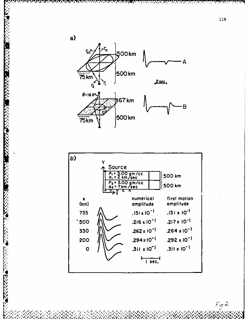
1Figure 2(b) shows a profile of Kirchhoff synthetics for a source 500 kilome-
ters above the interface and five receivers 500 kilometers below the interface.
The horizontal distance, x. of the receivers ranges from 0 kilometers, directly
-underneath the source, to 755 kilometers. The two columns next to the synthet-
ics contain the numerical peak amplitudes and the predicted amplitude from
.'4'-.. equation (15). The agreement is good. We cannot calculate a response past x =
755 kilometers because a truncation phase resulting from the boundary condi-
tions on the interface starts to interfere with the direct arrival. We must always
take care to avoid such contamination.
Ill. NTS Structure (An Example of Near-Source Effects)
We now apply the method by modeling the effects of idealised Moho struc-
tures on transmitted teleseismic P waves generated by nuclear tests in Pahute
Mesa, Nevada Test Site. We wish to ascertain whether focusing-defocusing by
structure on the Moho explains the unusual behavior of amplitudes from these
tests.
We review these anomalous observations of short period P waves from
*Pahute Mesa. Figure 3 is a plot of 1200 ab amplitude measi. 'ements from 25
tests within Pahute Mesa as a function of station location from Lay et al..
(1963a). The ab amplitudes are measured from the first peak to the first trough.
They are corrected for geometric spreading, the instrument gain at 1 second
and event size, following a procedure developed by Butler (1984). The ampli-
tudes are relative to a masLer event which minimises the overall scatter of the
data.
. . . ....... .... .... .._,,.. .'
AD-RA48 589 DETAILED OCEANIC CRUSTAL MODELING(U) CALIFORNIA INST OF 2/2TECH PASADENA SEISMOLOGICAL LAB D V HELMBERGER87 NOV 84 N88814-76-C-i@70
UNCLASSIFIED F/G 8/1@ NL
mEmmmmmmmEmmmmmmmmllmmmmmmmmmmmmEmEoE
92
The data has two important features. First, the relative amplitudes range
from .13 at station TRI to 5.1 at station SHK. This variation is nearly a factor of
40. Most stations between the azimuths 0' and 60' have significantly lower
amplitudes than those between 60' and 1200. Secondly, the relative amplitudes
at a given station vary by a factor of 2) as a function of event location within the
mesa. The latter variation clearly originates from a near- source mechanism
because the events are separated by. at most. 15 kilometers.
If one calculates the mean relative amplitude at each station, then the
overall amplitude variation with azimuth reduces to a factor of 12 (Lay et al..
1983a). The next two figures suggest that this large amplitude scatter is also
caused by a near-source mechanism. Figure 4. from Lay et al., (1983a), show,
the azimuthal pattern of relative amplitudes for GREELEY, an event within the
mesa, and FAULTLESS, an event 100 kilometers outside the mesa. Although both
" ~. events have comparable yields, their azimuthal patterns differ substantially.
This difference is particularly obvious between 0* and 90* . Figure 5 displays
plots from Lay et al., (1983b) which enhance the difference between patterns of5.--A- events in the mesa and events outside the mesa. These plots are ratios of ampli-
tudes of three events outside the mesa (FAULTLESS. PILEDRIVER, and BILBY)
divided by the average mesa amplitudes. These ratios are an approximate
measure of a near-source anomaly if the FAULTLESS, PILEDRrVER. and BILBY
O patterns are only influenced by path and receiver effects and are, therefore,
constant as a function of azimuth. Furthermore, the path and receiver effects
must be characterised by multiplicative factors. Because the ratio patterns for
all three events are similar, these assumptions are probably true. Therefore the
factor of 13 variation of these ratios between 00 and 120 is roughly an estimate
-p.
S.%% %%N- '-S.SP 6 % %
, . .93
of the near-source anomaly at the mesa.
To see if this amplitude variation correlates with waveform changes, we plot
in Figure 6 several seismograms at stations between 30' and 100* which
recorded both FAULTLESS and GREELEY. The top and bottom seismograms are
recordings of FAULTLESS and GREELEY, respectively, with their absolute ab
amplitudes in millicrons, corrected for instrument gain only. There is no obvi-
ous waveform differences in the GREELEY records which correlate with the
.dramatic ab amplitude changes. Furthermore we do not see any obvious
difference in frequency content and/or complexity between low stations and
high stations for either event. However there are some systematic differences
between GREELEY and FAULTLESS seismograms. A shoulder occurs 2 to :1
seconds after the first arrival on GREELEY records (e.g. STU, PTO, MAL. STJ, OTT.
CEO, and ATL). Lay has also seen these arrivals for other mesa events (Lay et
al.,1983b). No such arrival is apparent on the FAULTLESS seismograms. Also the
width of the first pulse of GREELEY seismograms is narrower than those of
-U. FAULTLESS seismograms at a few stations (e.g. SJG. ATL, BLA. CEO, SCP, and
STU). Both phenomena, though, occur throughout the azimuthal range and do
not correlate with the ab amplitude changes.
The data demonstrates that near-source anomalies cause a variation of 2k
of relative ab amplitudes at a given station as a function of event location within
. the mesa. Moreover, near-source anomalies also cause part of the large ab
- amplitude variation with azimuth (or station location) from mesa events. We
cannot completely eliniinate conitaminatio of the azimuthal pattern by path
and near-receiver effects. Certainly near-receiver effects can be as large as
those observed for the Pahute mesa tests (Butler,1984). Yet the similarity of
94
the ratio patterns of FAUL T LESS. BILBY. and PILEDRIVER suggests that the pat-
tern for mesa tests, seen in Figure 3, is dominated by a near-source mechanism.
Finally the variation or relative ab amplitudes with azimuth does not correlate
with any obvious waveform changes for a typical mesa event. GREELEY. There is
no definitive evidence to determine whether ab variations correlate with travel-
time residuals.
* 4 In this paper we assume that all the observed amplitude anomalies result
from near-source mechanisms. We then test the hypothesis that structure on
the Moho, consistent with travel-time residuals, focuses or defocuses P-waves
enough to produce the magnitude of the amplitude anomaly. There are alterna-
tive near-source explanations for these anomalies. In addilion, to the focusing-
defocusing hypothesis, workers (Lay. et al., 1983; Wallace et al.. 1953 ) postulate
that the movement of faults associated with nuclear blasts causes a superposi-
tion of distributed or point double-couple sources with the isotropic bomb
source. The amplitude anomalies are, then, the radiation pattern caused by a
double-couple source. Longer period studies of Love/Rayleigh ratios, Pnl, P and
S waves (Aki and Tsai, 1972; Wallace et aL., 1983; Nuttli, 1969) generated by these
blasts support the latter hypothesis. However, we speculate that, as the fre-
*.'. quency content of the signal increases, the role of lateral near-source structure44,
in distorting amplitudes becomes more important. From travel time residual
studies (Minster et al., 1981; Spence, 1974) workers have deduced that there is a
high velocity zone directly beneath the Silent Canyon Caldera in the mesa whichVe
extends down to 100 kilometers. Such a velocity structure may cause ampli-
O tudes which deviate from those predicted by a spherically symmetric Earth
model.
-, - . . V
ITXA
95
To investigate how geology can affect amplitudes, we presume that the
apparent velocity variations deduced from the travel time residuals are a man-
ifestation of Moho topography. We exclude from consideration the impact of the
Silent Canyon volcanics on transmitted P waves because both Spence and Min-
ster correct the residuals statically for these low velocity rocks; thus the resi-
dual patterns are not a result of the caldera. In any case, we cannot readily
model a feature so close to the source. If we place a strong velocity discon-
- tinuity ,such as that between volcanic and granitic rocks, closer than 10 kilome-
ters to the source, we generate a truncation phase which interferes with the
transmitted P phase.
We describe the Earth with a two layer crust-mantle velocity model. Thr
velocity of the upper layer is 6.5 kn/sec and that of the lower layer is B km/sec.
The depth of the interface is 45 kilometers. The receivers are located at dis-
tances such that the L-amplitude decay corresponds to spreading at telese-R
ismic distances between 60* and 70* for a JB Earth (Langston and Eelmberger.
1975).
The number of ways to distort the Moho is infinite. We, therefore, restrict
ourselves to a few three dimensional topographies where the maximum height of
the anomaly is 10 kilometers and the maximum width is approximately 25
kilometers. The choice of these values, is based on both the Minster et al. (1981)
and Spence (1974) studies. They find an advance of f.25-.4 seconds for nearly
vertical rays from shots within the caldera. As these rays become shallow, this
advance lessens or disappears completely. From crude calculations, we esti-
mate that 10 kilometers of upward relief on the Moho will produce the required
timing anomalies of these i'ays. Furthermore, we confine the relief laterally so.
. .,. % . p% % . p . ,.* . .%° %, % . . ,
* 96
that rays exiting the mesa at shallow angles are unaffected by the structure. We
recognize that these structures are extreme. However, if we cannot produce the
observed amplitude anomalies with these topographies, we can discard struc-
ture on the Moho as the dominant cause of these anomalies.
Of the infinite number of structures, we arbitrarily select four examples
with height c = 10 kilometers and width w = 25 kilometers. These topographies
are described by simple analytical formulas and are convenient to use. The
topographies with their labels are as follows:
Z Z Z,.. + -(cos(2r((r-w/2)/w))-1) ifr - -2 2
Z Z=.. if r > -T (7
Exponential :Z =Zc. - ce 2 (17a)
S'- Z = Z..n - c if r!5
plug.: Z = Z... + !_-(cos(2r((r--- 5)/w))-1) if E-<r5 !E-+ 5 (17b)
' ""Z = Z,,n if r> x-+ 5
21 99 1r(1c'-'." Sinc :Z =Z,,o, - c sinc [ 2191] 1c
H ere r = v(z -xz ), + (y,) and is the horizontal distance of each point on the
surface from the midpoints of the grid (Zc.y). Zon is the baseline level of the
Moho and is 45 kilometers for all the calculations. The values of the constants in
the exponential and the sinc bumps confine the anomaly's width to approxi-
*" mately 25 kilometers. A schematic cross section of each topography is shown in
Figure 7. All the structures are symmetric with azimuth.
" % ".,.-0 .' ''' , ' , - '"," . . '' .'. " . "@ ° " , 4 " ,', .,€ " @ J '€ € 4 ' '" . *' ..* ," , , . . .. .,. -.. ,.. ., . , ., ,' ,.' • ,•S. , , , ' ; , .. . , , ,
' 97
* Initially an isotropic source is directly above the center of the structure;
thus, the transmitted potential is only a function of x and z. The source is 45
kilometers above the baseline of the Moho. The transmitted potential is calcu-
lated at receivers which are 20,000 kilometers below the source. The horizontal
distance of the receivers from the center of the topography ranges from 0 to
7.000 kilometers. Figure 7 shows the transmitted potential and the peak ampli-
tude as a function of x in increments of 1.000 kilometers for each of the four
topographies. In addition, the responses for a wave which transmits through a
planar boundary are displayed in the first column. The corresponding take-off
angle for the fiat boundary synthetics are to the left of the column. By compar-
ing these synthetics with those in the other columns, we can determine huw
much distortion of the waveform is caused by each structure. The synthetics in
Figures 7 and 10 do not include a Q and instrument operator or a reflected pP
phase. Although these effects are important, we want to examine amplitude and
waveform distortions caused by structure with a simple input pulse. The ringing
caused by an instrument or pP may mask the presence of multiple arrivals
caused by the topography.
All the structures cause intriguing changes in the waveforms and arrival
times of the synthetics. The waveform features originate from timing changes
caused by each topography. Each point of the Kirchhoff synthetic originates
from elements which are illuminated by the source and, in turn, illuminate the
receiver at a total travel time, =Tri+r 2 . We can associate, with each element of
":". the grid, a value of total travel time. o(z.y). The total travel time function on
A' the surface depends on the source location, the receiver location, and the sur-
face geometry. Figure 8 shows examples of this function. Here we calculate.-'.
% %
%%? %
98
'(z.yO) for elements which make up a flat interface 8(a), an upwarped interface
B(b). a plug B(c). and a sinc function B(d). In each example the source is directly
above the center of the structure and is 45 kilometers above the baseline of the
interface. The receiver is 20.000 kilometers directly below the source. The con-
tours of constant total travel time are projected onto the topography (top
figure in 8(a),(b).(c), and (d)). We also display these contours as a function of x
r and y (bottom figure in 8(a),(b).(c). and (d)). The contours are circles because
of the particular source-receiver geometry. For the sake of brevity, we only
show that portion of the grid which contributes to the initial second of each Kir-
N4 chhoff synthetic. The synthetics which correspond to these total travel time
functions are also shown (middle figure in 8(a).(b),(c),and (d)). These figuies
show how structure on the interface distorts the total travel time contours and,
as a result, produces multiple arrivals in the synthetic.
We examine this effect in detail. The contours are in intervals of .125
seconds as are the tick marks below the synthetics in Figure B. The geometric
arrival time occurs at the center of the contour plot. Thus, by counting the con-
tours. we can estimate the cumulative area of the surface which contributes to
the synthetic at a given time. We deduce, from Figure 8, that, approximately,
A (t a S -I
A(t) is the amplitude of the response at time t. S is the total area of the surface
which contributes to the response at time t. For example, the initial .375
seconds of the synthetic from a flat interface results from a rapid increase in
V~e the cumulative area of the surface which is illuminated between t=.125 and
t=.25 seconds. After t=.25 seconds, the area of the surface is illuminated at a
%%_
99
constant rate. Thus, the resultant synthetic can be viewed as a convolution of
the source time function with a step function which starts between t=.125 and
.25 seconds.
We quantify this statement by following an approach developed by Hilter-
man (1975) and Haddon and Buchen (1981). The symmetry of the source-
receiver geometry and the surface geometry allows us to recast the integral
(13) as a one dimensional integration with respect to total travel time, a. If the
'..•transmission coefficient varies slowly over the surface, then
7Tfo( "z•(19)
where
dfl1 = dS
and
C osf32dO,1 rO0 dS.
-, and 62 are the time derivatives of modified solid angles. f0, is a modified solid
angle with vertex at the source subtended by the surface S. and 0 2 as a modified
solid angle with vertex at the receiver subtended by S.
We now examine the origins of the multiple arrivals in the potentials which
propagate through interfaces with structure. For example, the amplitude and
*frequency content of synthetics from the upwarp (column 3 of Figure 7) are
controlled by the interference of two pulses. The travel time contours in Figure
S.%,%
%
.I~- -. a-
100
7.
8(b) for the upwarp differ considerably from those of a flat interface 8(a). Far
less of the upwarped surface is illuminated within .25 seconds of the geometric
arrival time. Furthermore, the upwarp topography causes subtle changes of the
width between travel time contours. There are two locations where this change
occurs: 1) at the top of the upwarp and 2) at the edge of the upwarp. The first
pulse in this synthetic originates from the elements in the first location while
the second pulse originates from the second location. Because the ring of ele-
ments which contribute to the second pulse has a larger area than that of ele-
ments which contribute to the first pulse, the second pulse is larger than the
- first pulse.
As the receivers move away from the center, the maximum amplitude-
-decrease as a result of the interference of the two pulses. We destroy the sym-
-- metry of the surface illumination by moving the receivers horizontally. The
llumination of elements, which initially was simultaneous, now occurs at slightly
different times and causes destructive interference; this destructive interfer-
ence causes a reduction in peak amplitudes and the broadening of the pulse
widths for both phases. Moreover, as the receiver moves out laterally, the
planar part of the boundary becomes more important in controlling the ampli-
tude of the transmitted pulse. Hence the amplitudes, travel times, and the
waveforms of distorted pulses approaches those of a pulse which has propagated
through a flat boundary. This phenomena is present in almost all the top syn-
thetics in Figure 7.I, Other intriguing features are present in the synthetics shown in Figure 7.
The potentials transmitted through the sinc and exponential bumps shown in
columns 3 and 5 have an apparent delay which is nut seen in the other
..- ,'...a ..
% %",a''b' : . ._, , ;¢,L' .;,.'. ," ".' :"'.-',.-."..",.":"'' .' .,v...., . - ..
III F
101
synthetics. These two topographies drop in height near the peak more rapidly
than does the upwarp topography. Consequently. fewer elements are
illuminated and contribute to the transmitted potential at times near the
geometric arrival time. This is illustrated for the sinc topography in Figure 8(d).
Hence, the amplitude near the geometric arrival time is lower than amplitudes
at later times.
The opposite is true for the synthetics of waves which are transmitted
through a plug. They are displayed in column 4 of Figure 7. The topography and
travel time contours for the bottom synthetic from this column are shown in
Figure B(c). This figure shows that more elements are illuminated and contri-
bute to the response near the geometric arrival time for this topography than
'p for the upwarp, sinc, and exponential topographies. The resultant synthetic is'.
made up of two pulses of equal size. Each pulse has the amplitude and shape of a
wave which has transmitted through a planar interface. The plug is essentially
comprised of two planar interfaces, one at z = 45 kilometers and the other at z
,. - 35 kilometers. The edges of the plug have been tapered to avoid a shadowing
problem. While the difference in the interface depths does not alter the ampli-
tudes of the pulses, it does change the arrival times. This slight separation in
arrival time causes the observed interference pattern. As the receiver moves
out laterally, the timing between the two pulses changes. The pulse width of the
first arrival narrows while the width of the second one broadens. By transmit-
ting a wave through such a structure, we vary the maximum amplitude of the
synthetics by a factor of 2 .
We confirm that these structures are approximately producing the correct
travel time anomalies. We plot the residuals, in addition to the peak amplitudes
•.4
9?. 102
-. , of the synthetics, as a function of distance to discern any systematic relation-
-" ship between the two parameters. We also plot the amplitude of the first pulse if
the synthetic is made up of multiple arrivals. This amplitude is measured from
the start of the synthetic to the first peak. The plots are displayed in Figure 9.
The travel time "residuals" are defined by the difference between the arrival
times of transmissions through a bumpy surface and the times of transmissions
through a flat surface. Where there is an apparent delay in the synthetics such
as in those from the exponential and sinc bumps, we measure the arrival time at
the start of the upswing. The amplitudes are uncorrected for geometric spread-
ing. The change of amplitude from spreading, seen in the synthetics in column 1,
is negligible in the distance range of interest; hence no correction is necessary
The "residuals" in Figure 9 produced by these structures behave in a
predictable fashion. The transmitted potentials which propagate vertically to
stations between 0 to 4,000 kilometers experience the most advance. The
exceptions to this behavior are residuals from the sinc and exponential synthet-
ics. We know there is some energy arriving at these nearly vertical stations with
.3 second advance from the previous discussion. However, because the energy is
so small relative to later pulses, these synthetics appear to have delays.
When the paths of the potentials become shallower, we see that the advance
disappears. The planar part of the interface begins affecting the travel times
and waveforms. The arrival times of the transmissions through the bumps
approach those of transmissions through a flat interface. The exception to this
advance of .3 seconds which is constant as a function of horizontal distance.
This behavior results from the constant. height of the plug across the entire
a'.
ON4 % % S ./ f- a. . .. ,-, ' %
- . ..'. > . , . WF . V . ', 'Pe *' J ',.'. 7 ' . " '-"- " " " ,; . . - '- - -" "-" - - - ' -
" "
103
width of the bump.
What is the relationship between the travel time anomalies and the ampli-
tude anomalies? We predict that as the magnitude of the travel time anomalies
decreases the magnitude of the amplitude anomalies decreases also. The ampli-
tudes, as well as the arrival times, will be controlled by the planar part of the
surface. This relationship is observable in Figure 9. The amplitudes, except in
one case, start to approach the value of .002 tt distances ranging from 5,000 to
7,000 kilometers. The exception is the maximum and first pulse amplitudes of
* the synthetics from the plug topography. These values appear to systematically
decrease with distance. However these values do approach the planar ampli-
tudes at distances beyond 7000 kilometers.
Furthermore. waves which arrive earlier than is predicted by planar calcu-
lations also have lower amplitudes than is predicted. Contrarily, the synthetics
from the sinc topography arrive late and have anomalously high amplitudes.
Indeed, the pattern of residual variation is precisely mimicked by the pattern of
amplitude variation for this structure. The mimicking of amplitude and travel
-" time anomalies also occurs for synthetics from the exponential bumps.
This mimicking does not occur for synthetics from the upwarp and plug
topographies. Each of these synthetics consists of multiple arrivals. Thus, if we
L%.10% take the maximum amplitude as a measure of amplitude anomaly and compare-
with travel time anomalies, we do not see an obvious correlation between the two
parameters. The travel time is perturbed by a relatively small part of the sur-
face. The maximum amplitude is perturbed by a much larger part of the sur-
face. It is a less local property of the topography. If a broader band source
time function interacts with the surface, the amplitude anomaly would change
io---
104
but not the travel time anomaly. To improve the correlation, we measure the
amplitude of the first pulse of the synthetic if it is different from the maximum
amplitude. These values are shown in Figure 9 by the open circles and triangles
for the upwarp and plug synthetics. We do not improve the visual correlation
significantly.
The modeling of a symmetric structure demonstrates that such a structure
on the 1koho, consistent with travel time residuals, causes a factor of 2X in max-
imum amplitude variation as a function of distance. The variation of amplitudes
of first pulses is somewhat less. Neither variation is as large as the observations
of amplitude changes between stations for a given test at NTS. Furthermore.
where there is a large amplitude variation, there is significant waveform distor-
-.-- tion of the synthetics. Also, the bumps generally cause low amplitudes. We note
that the mesa data set has both anomalously high and low amplitudes. The low
amplitude synthetics arrive early. However, any relationship between amplitude
anomalies and travel time anomalies is dependent on frequency because the
effect of a structure on a wave is dependent on frequency.
- The modeling to this point produces anomalies which are dependent only on
distance because the structures are symmetric. We now introduce asymmetry
into the problem by allowing the source to move off the center of a symmetric
upwarp. We do these calculations because observed travel time and amplitude'0
anomalies are presented as a function of azimuth. Yet we do not know if these
anomalies arise from azimuthal or delta heterogeneities. Additionally, there is
an observed variation of amplitude at a given station with a change in source,0
position in the mesa. If we change the source position across a sample struc-
ture, can we reproduce the factor of 2) seen in Figure 3? We also wish to. $i,,.-9-_
Xr N4
105
'I'
examine whether there is any systematic relationshin between amplitude and
. ;travel time anomalies as a function of azimuth as we have done previously with
these parameters as a function of distance.
The modeling experiment is similar to the previous one. The receivers are
1000 to 7000 kilometers horizontally away from the center of the topography
and 20.000 kilometers below the source. The sources are 45 kilometers above
the baseline of the Mohu. To produce the azimuthal anomalies in the synthetics.
we move the source off the center of the upwarp in one direction in increments
'P, of two kilometers. The responses are calculated for seven distances at five
*' different azimuths. We select the topography upwarp for this experiment. The
choice of topography is somewhat arbitrary; however, we make this particular
choice because this topography causes substantial variation in amplitudes as a
function of distance.. If this topography fails to produce much azimuthal varia-
tion, then the other topographies will fail to do so, also.
Figure 10 shows our results. A cross section of the source-receiver
configuration and the geometry of the upwarp is in the center of the figure. In
addition, a topographic map of the center portion of the grid is displayed. The
contours are in kilometers and the maximum height of the bump is 10 kilome-
ters. The topography map also shows the source locations and the azimuthal
lines along which the calculations are done. The resulting waveforms and max-
imum amplitudes surround these diagrams. Each group of 28 waveforms is cal-
,- '.culated for the corresponding azimuth. The groups are made up of four columns
of synthetics corresponding to calculations done with the source location desig-
nated at the top of each column. Sources A. B. C, and D are, respectively, 2, 4, 6-5%
and 6 kilometers from the center. The rows correspond to calculations done at
-5,',',.... - ,,'--. ",;. '.''" ; * .. .,..' -_. " ,-.. ' :' .. ""*.*w '***.-..' ' '....;..,".' ', ;- '.'''',''' ,,,,'"l',..'% "'
O: 106
the horizontal distances next to the row. In Figures 11, 12, and 13 we plot the
travel time residuals, peak amplitudes, and first pulse amplitudes obtained from
these synthetics as a function of azimuth for each distance.
There is a change in overall complexity of the synthetics as a function of
azimuth. The waveforms from the group at 0 =00 are simple and impulsive with
relatively high amplitudes. Only the stations at 1.000 or 2.000 kilometers have
multiple arrivals. As we rotate counter-clockwise around the structure, a
greater number of the synthetics in each group have multiple arrivals, and con-
0 sequently, low amplitudes. Synthetics at e= 1351 and 1800 all have multiple
arrivals. The reason for this trend is the same as in the previous modeling study.
As the sources move in the direction of a line along e= 00. a greater proportioI
of the elements which constitute the planar part of the grid contribute to the
potentials calculated in the direction of this line. Hence, synthetics of this line
become more impulsive as the source migrates from position A to position D. In
contrast the synthetics at e= 135" and IB0 0 remain complex. The elements
which contribute to these potentials are largely from the non-planar part of the
boundary.
60 We examine the maximum amplitudes, first pulse amplitudes, and travel
time residuals in Figures 11, 12, and 13 for systematics as a function of distance
or azimuth. The behavior of maximum amplitude with distance and azimuth is
-, the most variable of the three parameters. The maximum amplitudes as a func-
tion of azimuth do not correlate very well with the travel time residuals. The
rapid change of this parameter with azimuth and source position reflects the
6sensitivity of maximum amplitudes to slight changes in relative timing between
,>-' the two arrivals which make up the synthetics. The least variation of maximum
M".N
',:-:....'':.'.:''., '#,..'-',,..,sf 3 'w ' .,.'. :,' .:'":.:. ,: ::.'..':; n&; -:,',...,.N''';:.j;A, . ;
107
amplitudes with distance and azimuth occurs at synthetics calculated with
source position A. the closest source to the center of the symmetric source. We
increase this variation with azimuth and distance when we remove the source
further away from the center to positions B. C. and D.
The maximum amplitudes at 1 = 135* for source positions B. C. and D are
lower than the amplitudes at other azimuths. This trend is a result of I) the
degree to which the planar part of the grid contributes to the response and 2)
the degree of symmetry of the source and receiver locations with respect to the
structure. Stations along e = 01 and 0 = 1 0B are in positions of symmetry withI
respect to the sources. Elements on either side of a line which divides the grid
contribute simultaneously to the responses at these stations and ,consequently.
cause higher maximum amplitudes. Stations along 9 = 90* and 09= 45* are not
symmetrically positioned with respect to the source; however, the planar part of
boundary largely contributes to these responses; thus, they have high maximum
amplitudes. But receivers along e = 135* are placed asymmetrically which
causes elements to illuminate at different times; in addition, these elements are
*i largely in the perturbed part of the boundary. These two factors combine to
produce the overall lower maximum amplitudes of receivers at 6 = 135 ° .
Although we do not discern any relationship between the maximum ampli-
tudes and the travel time residuals as a function of azimuth, we see a correla-
tion between the first pulse amplitudes and the travel time residuals. Synthet-
ics which have a constant first amplitude as a function of azimuth also have
approximately constant travel time residuals. When the travel Linite oidvances
increase as a function of azimuth, the first amplitudes decrcase with azimuth.
Thus, early synthetics have lower first amplitudes than the later synthetics. The
a~~~F F F ** *
* -"*.*'*'° . 'S. * . . . '_- .*
-.0 108
trend of early arrivals with low amplitudes and late arrivals with high amplitudes
holds true for all azimuths, distances, and source positions.
The travel time residuals decrease as a function of distance at aU azimuths
except for e= 1350 and e = 160* for sources C and D. At these azimuths, the
residuals increase as the distance increases. Clearly if we pull the source off the
center far enough, the shallower rays will interact with the upwarped part of the
topography while the steeper rays interact with the fiat part of the grid.
-, As the source moves off the center, the range of variation of first ampli-
tudes and travel time residuals as a function of azimuth exceeds the range of
these parameters as a function of distance; that is. the trends of these parame-
ters are stronger in azimuth than in distance. Thus, stronger variation of travel
time and amplitude anomaly with azimuth than with distance may be an indica-
tor of lateral variation with azimuth, as well as with distance, despite an uneven
station distribution of the existing data set.
What conclusions can be drawn from this modeling experiment? Firstly, we
create a variation of 2X of first amplitudes as a function of azimuth and source
* position. The change of amplitude with source position is largest at
-= 0 and 45 o and is the least at e = "180. However, the variation at 0* and 45 o
is created at the cost of considerable distortion of the waveform. This feature of
low amplitude waveforms with complex or broadened pulses and high amplitudes
waveforms with simple narrow pulses is not apparent in the mesa data set.
Secondly, we create a trend in the first pulse amplitudes with azimuth.
* Specifirally we cause high amplitudes at e= 0* . 1350 , and 1800. If the source
moves far enough away from upwarp, it causes no amplitude anomalies. How-
ever structure can produce a systematic azimuthal trend in amplitudes. But we
A" -LA
109
must be cautious about pushing this interpretation too far. The azimuthal trend
is an artifact of the moveout of the source in one direction with respect to the
lines of receivers. If we were to distribute sources all over the upwarp and then
calculate the averages of the first amplitudes at each azimuth for all the
sources, we would undoubtedly eliminate any trend with azimuth. Thus, the sta-
bility of the amplitude pattern of all mesa events with azimuth location is not
easily explained by structure on the Moho or any unusual velocity plug unless
the sources are fortuitously located to one side of the heterogeneity.
* Thirdly, we see a visual correlation between travel time residuals and ampU-
.% Ludes of first pulses, but do not see any between residuals and peak amplitudes.
This correlation may be diagnostic of structure as opposed to tectonic release.
* Discussion and Conclusions
The previous two modeling experiments show that a structure on the Moho
which causes travel time residuals compatible with the Minster et al., (1981) and
the Spence (1974) studies can produce variations of 2)j of amplitudes as a func-
tion of delta, azimuth, and source position. The variation is created at the cost
-* of considerable distortion of the waveform. Furthermore the travel time residu-
als correlate with first pulse amplitudes but not with peak amplitudes. To see
whether these initial results are relevant to the Pahute Mesa waveform data, we
-• must now include a pP phase, a Q operator and a short period instrument opera-
tor in a few Kirchhoff synthetics.
V" We choose two sets of five Kirchhoff-Helmholtz synthetics calculated at 4000
* kilometers previously for the azimuthal study. The two sets correspond to the
source positions A and D at five azimuths. This choice represents two extremes
p
:. % 0
110
of source positions relative to a structure and may give us a reasonable idea of
what to expect in amplitude and waveform variation as test sites move within the
mesa.
We put pP into the Kirchhoff-Helmholtz synthetics by convolving these syn-
thetics with a boxcar function of unit height and a width corresponding to the
pP-P lag time. This convoluLion yields the impulse response of P and pP if the
incident source is a modified Haskell function rather than its time derivative.
We justify this simple model of pP by assuming that the reflection coefficient of
this phase is -1. Lay et al. (1983a) estimates the reflection coefficient as .96 for
pP. We further argue that pP interacts with the same part of the surface as does
P. This assumption is good for the shallow depths of the mesa tests which rangt
from .5 to 1.4 kilometers. The width of the boxcar is .85 seconds; this estimate of
the pP - P lag time is taken from Lay et al. (1983). A short period instrument and
a Futterman Q operator is also convolved into these synthetics. We use a Haskell
function with parameters (D = 2.K = 10) while Lay et al. (1983a) use slightly
F, different values (B = 1.K = 8).
* Figure 14 displays the results of the convolutions. The first column con-
tains the initial Kirchhoff-lielmholtz synthetics with peak amplitudes taken from
Figure 10. The second column show these synthetics convolved with a AWSSN
short period instrument and a boxcar. We introduce additional complexity into
the waveform but do not change the range of peak amplitudes significantly when
-- we include an instrument and pP. The complexity of the waveform caused by
structure is masked by the dominant interference between P and pP.
% We next convolve these synthetics with Futterman Q operators with a t* of
%e .5 and 1. The waveforms and their ab amplitudes are displayed in columns 3 and%%d% %
%9-
"°""."e " • • " " " " ,'-" " , *, -. ..*.'. ", " . .~." "" ... " ."%," ". *. '""" ' " " --2' , ",-4 '.e ,., ,.,., ,.e• o%° • %° 'o• .. % ., o .. . - o " % -. . . o , . . ° - ,• o -, -- " w ! - , ,-.
" " 111
4. The ab amplitudes are plotted as function of azimuth for both sources and to
values In Figure 15. We remove the complexity of the waveform for both sources
with the two to values. However there are some observable differences in the
*- .- first and third peaks of the waveforms as a function of azimuth. The first peak
widens as azimuth increases. The third peak becomes smaller and disappears
altogether. Moreover. Figure 15 shows a variation of ab amplitudes with azimuth
-, of 2)j for source D if t° is .5. However, when t° is 1. this variation reduces to a
factor of 1.7. We also obtain a variation of 2X of ab amplitudes with respect to
source position if t° is .5. This occurs at 9 = 0* and e= 450; however the
"-$ difference between ab amplitudes for the two sources decreases as the azimuth
increases.
Thus we cannot predict the observed ab amplitude variation with azimuth
or station location if we use a structure on the Moho 10 kilometers high and
approximately 25 kilometers wide. If the factors of 12 or 40. seen in Figures 3.
4, and 5, are measures of a purely near-source phenomena, then one requires a
structure several hundred kilometers in scale on a boundary to match these fac-
tors. This structure would distort the waveform considerably. Yet there is no
obvious evidence in the observed seismograms for a correlation between low
J amplitudes and complicated and/or broadened waveforms or high amplitudes
and simple, impulsive waveforms. We speculate that. rather than a large struc-
ture on a single boundary, a small velocity or density perturbation along a
several hundred kilometer ray path may produce the desired amplitude change.
iA_ However we cannot test this speculdtion with our method.
* On the other hand, we predict a factor of 2X in ab variation with source
location if to is .5 . This variation is not accompanied by any significant
-' % N
A. - A*** % ~ ~~' V * % A % p~
112
pp'-
waveform distortion. Although we only produce a factor of 2f at two azimuths,
this is an artifact of the source moveout across the structure. If sources were
uniformly distributed over the structure, we would cause this same magnitude
of variation at all the azimuths. Furthermore. no source would be systematically
higher in ab amplitudes than another source at all the azimuths. Unfortunately
Figure 3 does not show systematics with respect to source location. The data
should be examined for such trends.
Also the travel time residuals do not correlate with the ab patterns. The
, convolution with two t* values demonstrates the frequency dependence of the
. 'phenomena. If t* is larger than 1, we will produce a flat pattern of ab amplitudes
with azimuth but the travel time residuals will not change. Thus we do not
expect a systematic relationship between travel time and ampLitude anomalies
because the ab amplitudes are sensitive to Q but the travel times are relatively
stable. This is an unfortunate result because such a correlation would be diag-
nostic of structure as opposed to tectonic release. As yet, there has been no
study which definitively demonstrates a relationship. In addition the data sets
-. of amplitude and travel time measurements do not have a one-to-one correspon-
0dence. Lay et al. (1983a) measure the ab amplitudes off of short period W SSN
instruments while Minster et al. (1981) and Spence (1974) use culled travel time
measurements from the ISC catalogs. We clearly need a study which compares
- the travel time and amplitude from the same seismogram.
The largest overall variation in ab amplitude with azimuth in Figure 15
occurs because of differences in t* values. Yet there are no noticeable changes
in the waveform. Thus the ab amplitudes are far more sensitive than waveforms
to Q differences. Perhaps, a lateral variation of Q with path can produce the
- % %A&.
113
extreme scatter of ab amplitudes for both tests inside and outside the mesa.
However it cannot explain the diferences in patterns between these different
test site areas. If the near-mesa anomalies are ,indeed, at least a factor of 10,
then structure on the Moho which is compatible with travel time residuals can-
not produce these large variations of amplitude with azimuth. However such a
structure could explain the observed variation of ab amplitudes with source
position at a given station.
,... .. . . ., . .. ,.,, .. , . .. ,-..,. .. .-.=.=.:, '. ,.''..'.,.,''.' .'.,'
'S" 114
References
Aki. K. and Y.-B. Tsai (1972), "Mechanism of Love-wave excitation by explosivesources". J. Geophys. Res.. 77, 1452-1475.
Butler, R. (1984). "Azimuth, Energy, Q and Temperatures: Variation on P waveamplitudes in the United States", Review of Geophysics and Space Phy-sics, 22. 1-36.
- Haddon, R. and P. Buchen (1981). "Use of the Kirchhoff"s formula for bodywave calculations in the Earth". Geophys. J. R. astr. Soc., 67. 587-599.
.' Hilterman. F. (1975). "Amplitudes of seismic waves - A quick look". Geophys.,40, 745-762.
Hong. T. L. (1978). Elastic WavJe Propaigation in Irregular Structures.(Thesis, California Institute of Technology).
Langston, C. and D. V. Helmberger (1975). "A procedure for modelling shallowdislocation sources", Geophys. J. R. astr. Soc.. 4.2, 117-130.
Langston, C. (1977), "The effect of planar dipping structure on source andreceiver responses for constant ray parameter", Bull. Seism. Soc. Am.,67. 1029-1050.
Lay. T., T. C. Wallace. and D. V. Helmberger (1983a), "The effects of tectonicrelease on short-period P waves from NTS explosions", Bull. Seism. Soc.Am.. 74, 819-842
Lay, T., L. J. Burdick, D. V. Helmberger, and C. G. Arvesen (1993b), " Estimat-ing seismic yield and defining distinct test sites using complete waveforminformation", Woodward-Clyde Report, WCCP-R-84-01.
Minster. J. B., J. M. Savino, W. L Rodi, T. H. Jordan, and J. F. Masso (1981).-a- "Three-Dimensional velocity structure of the crust and upper mantle
beneath the Nevada test site", Systems, Science, and Software Report,SSS-R-O 1-5138.
Nuttli, 0. W. (1969). "Travel times and amplitudes of S waves from nuclearexplosions in Nevada", Bull. Seism. Soc. Am., 59, 385-398.
Scott, P., and D. V. Helmberger (1983). "Applications of the Kirchhoff-Helmholtz integral to problems in seismology". Geophys. J. R. astr. Soc.,
" 72.237-254.
Spence. W. (1974). "P-wave residual differences and inferences on an upper% mantle source for the Silent Canyon volcanic centre, Southern Great
Basin. Nevada", Geophys. J. R. astr. Soc., 38. 505-523.
Stratton, J. A. (1941). Electromagnetic Theory, First Edition, McGraw-FillBook Company. Inc.. New York
Wallace, T. C., D. V. HeImberger, and C. R. Engen (1933). "Evidence of tectonicrelease from underground nuclear explosions in long-period P waves",
r . ~'IF~DV a* '~. P . W,%,.' ~~%
. * ,,ir - .*. . . . - -.-
' "116
Figure Captions
la. The geometry of the Kirchhoff-Helmholtz calculations for transmissionacross two acoustic media with sound speeds a, and a 2 and densi-ties p, and P2. The source is in V, at x and the receiver is in V2 at
*lb. A close up of a piece of the boundary which displays the angles.
2a. Two synthetics and the grid geometry used to compute them. Synthetic A iscontaminated by a truncation phase which originates from theedge of the grid. Synthetic B is contaminated by a phase whichoriginates from the abrupt change in boundary conditions. Thegrid next to synthetic B is gray when V = 0 on the boundary.
2b. A comparison between Kirchhoff-F.elmholtz and first motion solutions. Theinput source is the first derivative of a modified Haskell functionwith parameters (B=2.K=10). The maximum dimensionless ampli-tude of the source input function is 45.1 .
3. The short period P wave ab amplitude data set for 25 Pahute Mesa eventsplotted as a function of station location. The amplitudes arecorrected for event size, geometric spreading and instrument gainat 1 second and are plotted relative to a master event (from Lay etal.. I 983a).
4. The relative ab amplitudes of GREELEY and FAULTLESS as a function of sta-. t~ion location (from Lay et al., 1983a).
5. Ratios of relative ab amplitudes of FAULTLESS. PILEDRIVER. and BILBYdivided by the average relative ab amplitudes of the mesa events(from Lay et al.. 1983b).
8. Seismograms from FAULTLESS (top record) and GREELEY (bottom record)displayed in order of increasing azimuth in the range of 300 to100*. Also shown are the absolute ab amplitudes in millimicrons.corrected only for instrument gain at I second.
7. Transmitted potentials from sources 35 kilometers above the center of the.. structure. The cross sections of the structures upwarp, exponen-
tial. plug and sinc are above the synthetics. For comparisonpotentials which propagate through a flat boundary are shown inthe first column. The potentials are from receivers which are20,000 kilometers below the source and which vary from 0 to 7000
5%, kilometers horizontally away from the source. All amplitudes are
. . . ... . ..'e d ,a'W2w' w v'w, ,'W' " ," ";". -.- -w .. " :.e'.,:" ,'',.', ... ". ",", ", ,,",,',.." ."". ". .,".w e .,". ". ., € , "V,'w ,..:;"Stu- ,
-* 117
multiplied by .01.
8. Travel time contours for a source 35 kilometers directly above the structureand receivers 20,000 kilometers directly below the source. Thefour structures are a) a plane . b) an upwarp, c) a plug, and d) asine function. The contours are projected onto the topographiesand flat grids. The synthetics which correspond to each traveltime projection are in between the two projections. The contourinterval is .125 seconds as are the tick marks of the synthetics.The geometric arrival time is the center of the contours.
9. Plots of peak amplitudes, amplitudes of first pulses, and travel time residualsas a function of distance from synthetics in Figure 7. The differentsymbols correspond to different topographies and are at the bot-tom of the figure. Where first pulse amplitudes are different frompeak amplitudes, the values of first pulse amplitudes are plottedwith open symbols and the peak amplitudes are plotted with closedsymbols. The dotted line corresponds to the peak amplitudes fromsynthetics which propagate through a planar interface.
10. Synthetics from the topography upwarp calculated for four source positions,five azimuths and seven distances. The topography map and cross
. section with source positions are in the center. The contour inter-val is 1 kilometer. The distances. angles, and azimuths of thereceivers are also shown.
11. Travel time residuals for source locations A. B. C. and D plotted as a functionof azimuth and distance.
12. Peak amplitudes for source locations A. B. C, and D plotted as a function ofazimuth and distance.
13. Amplitudes of the first pulse for source locations A. B. C. and D plotted as afunction of azimuth and distance.
14. Kirchhoff-Helmholtz responses (first column) convolved with a boxcar of" width .85 seconds and a short period WWSSN instrument (second
-. column) and a Q operator with t" values of .5 (third column) and Ie. (fourth column). Responses are from a distance of 4000 kilome-
ters. azimuth range of 0* to 1800 and source locations A and D.
15. ab amplitudes from synthetics in Figure 14 plotted as a function of azimuthfor both source locations A and D and both t values.
- %o
-. %
i' 119
a)
pro, 00 km
OOkm75km 2 sec1
r r
-167 km0 -~km
75km 0kV: b)
YA. Source
'" l " km/sec 1500 kmPaz 3.00gm/ccat= z 7kin/sec 1500 km
x numerical first motion(kin) amplitude amplitude755 *A .15Ix 10 " 1 .151 x 10- 1
500 .216 x 10"1 .217x I0- 1
330 .262x 101 .264 x 10
200 .294x10" .292x10
.311 x 10 .311 x 101
I sec,
6
11." .."." .... .. ..."- "',. .% ''."""'","' "."" " v" '"..% '.,',_',.,1, '" J- ° """" % % "" ° " ""% %% % " ""° " ""1% % " "" " '%% % %" %"" "'
• = '% "-- % -- l -I - - - ., * ,
:. ' .' .- . " ._ , '_ , . ( ' '. ' .- : ' ,' - . './ :. , . ," ., . .. .. '-'. ... ,. .. .. :,.,- ,% t.- . ,? '--
'6 122
CL Faultless /Avg
> 1. *s
W 0.5 00-0
00
Piledriver / AvgCLE .o--- -- ------------------------------------------- 9 -----------
@3 0. 0 0
~0.5
CL Bilby /Avg
E 2.0 09 ------------- - --- ---- --- ----- --- - - -- -- ---
00
S0.5
0.0 60.0 120.0 160.0 240.0 300.0 360.0
%
124
(D - 0) *. Cj~
ccl
CD In l-- w~ w~ 0' 0
N co K
o 0 N - (
0. 0
00 0 (0 o o N o
0 0 000 0 000
ft w 0 In n N
(r.- K) 0 O' r-~0
-r V 'oe ro~ * *Nil
126
,. o first pulse A first pulse
- peak amplitude A peak amplitude
.3A
=_Jl .:2. _ .2 ....... .. ....... ....... A ................. .....
S0 0 0 0 002
06
-. 2
•-,,.. Distance (xlI0 kin)
11 I
4A
A"-' "m s in c 9 u p w rp:-: - g ussin A toperplug
OU ,** *
127
m m mCC= 4= 4= CD
m
*L u9wC?
0 =4 DCC= 4 = = = C n
fn fn *0q Nocn ci
<
E C5 CD U,*zc
*~ CID,
* , 'T V '
128
ResidualsAzimuth
00 900 1800 000 900 1800
S-02 ~ 02' -
- 0 . 3 . . ~.
-Oo2 .........
V.)
QO3 9010 1800 QO900 1800
CD 4.,\6 D
-0.2 -0.2
-0.3L4;2=2000 6 = 600
3 3000 7 =7000
1-
z %
-JW
129
Peak Amplitudes
Source AB0.2- 0.21
is7
4' 010.
(km) 2 4=400
2=2000 6=60003=3000 7=7000
I I I ICL 00 900 1800 00 900 1800E
-0 7 CaQ 0.2's-. 0.2
, F/*2
0 01
06
oa
130
* Amplitudes of First Arrival
Source A 7 00B
0.2- (kin) 0.2 5=5000
3 30007-.0,
2~0.17-5%
~r00900 1800 00 900 1800
0
(5I6i0 .7 56 D
0.2 7 u \ .
0..2
-4E
.42
00900 1800 00 900 1800
Azimuth
131
Source A(peakl (peak) .5 ab 1.0 aamop) ,amep (a°mp) ampl
Az. x O"3 X O-4 xlO x10-5
00 .82 1.01 2.90 1.17
'.450 .79 ]L .99 2.81J 1.17
90 .78 .87 2.91 1.17
135 ° .97 ) 1.18 3.53 1.25
180 ° 1.10 J 1.44 3.90 1.31
Source D 5 sec
00 2.23 2.61 6.40 1.82
450 1.99 2.34 5.92 1.71
900 1.20 1.43 4.14 1.30
135' .59 .76 2.85 1.15
1800 1.27 4 1.78 4.09 1 .24
J. J* /Pe/
132
7-O SOURCE A* SOURCE D
-t =.5::: --- t* =I-
5-
"""In
'o
c3
0
2.--"
- - -..- --
0o 900 1800azimuth
.- '.I' .'- , ,I ' ~~~~~ V.i ,- -. V - ' ' V' " -- ' % " "'J- %.'L % N,' % I I' .,.. %I I *F -. % -. 1. -
Z or . 5 e 4
* ECURIT', CA-SSIFICATION OF THIS PAGE
REPORT DOCUMENTATION PAGEI I -EPORT SECURITY CLASSIFICA1 ION 1b. HESTRICTIVE MARKINGS
21 SECL;RIT CLASSIFICATION AUTHORITY 3. OiSTRIBUTIONjAVAILABILITy OF REPORT
Seismological Laboratory-b. DECLASSIFICATION,DOWNGRAOING SCHEDULE California Institute of Technology____Pasadena, CA 91125
4 PERFICRMING ORGANIZATION REPORT NUMBERIS) 5. MONITORING ORGANIZAT;ON REPORT NUMBER(S)
N00014-76-C-1070
16a. NAME OF PERFORMING ORGANIZATION 6. OFFICE SYMBOL 7a.1 NAME OF MONITORING ORGANIZATION
California Institute of ,faippiicable, Office of Naval ResearchTechnology Resident Representative
uc. AODDRESS iLll' atae and 1IP CoJdeI 7b. ADDRESS '.ty. - Lote and 1IP Co')e
1201 E. Calif. Blvd. 1030 E. Green St.* Pasadena, CA 91125 Pasadena, CA 91106
- a NAME OF FUNOING,SPONSORING 8b. OFFICE SYMBOL 9. PROCUREMENT INSTRUMENT IDENTIFICATION NUMBER_RGANIZATION (d(applicoble)
Office of Naval Research NR 083-399
dc ACORESS .(%N, .itat' and ZiP Co&cI 10 SOURCE OF FUNDING NOS
800 N. Quincy St. PROGRAM PROJECT TASK vNORK UNIT
Arlington, VA 22217 ELEMENT NO. "J0 NO. NO.
-. " 1 1 ", TL: Inc,,a'&l" 3 Cur1I L~das41 aCa{I~onI
Detailed Oceanic Crustal Modeling12 PERSONAL AUTHOR(S)
Dr. D. V. Helmberger,ja. r P OF REPORT 13b. TIME COVE~RED 14CATE OF REPORT V, 'to.. L 1. AG CUN
.inal Report FROM -/18J 7o VL3I/84 1984 November 76 3 .PPLEME'JTARY NOTATION
.7 CCSATI CODES 18. SUBJECT TERMS IConflnue fin rcverqe If ncessa-' and identify by biocie numberl
",ELO RCUP SUB. GR.
19 ABSTRACT I 'ntmue ui everse f necessary and dentity by bfti number,
The research performed under this contract can be divided into 3 main
topics: changes in existing methods, Cagniard de-Hoop and WKBJ, which enableconstruction of synthetics for mixed path situations; use of long period SHwaves with source in the Northwest Atlantic and receivers on the northeastcoast of North America to derive an oceanic upper mantle shear velocity model;and a technique based on evaluating the Kirchoff-Helmholtz integral forpredicting the effect of near source or near receiver structure complexity onfar field p waves.
* 4.'In Section II we assess the fact that recent models of upper mantle
'. Jstructure based on long period body waves (WWSSN) suggest large horizontalgradients, especially in shear velocities. Some changes in existing methods
- L p .STRAI;T -CL'l 'I
* '.:.~..--=D Nt,~ ~ A j~ PT - 4CCLSERS
WI I 1 S a (- -
. Dr. D. V. Helmberger (818) 356-6998
-.D FORM 1473, .3 APR -C " o OF I. A. 7: S ";._ a.- _
" -"'..a r -., or.",,IS PAGE
-- % .6 % . %m %~
SECURITY CLASSIFICATION OF THIS PAGE
are required to construct synthetics for mixed path situations. This isaccomplished by allowing locally dipping structure and making somemodifications to generalized ray theory. Local ray parameters are expressedin terms of a global reference which allos a de-Hoop contour to beconstructed for each generalized ray witi the usual application of theCagniard de-Hoop technique. Several useful approximations of ray expansionsand WKBJ theory are presented. Comparisons of the synthetics produced bythese two basic techniques with known solutions demonstrates their reliabilityand limitations.
In Section III, we have modeled the SH motion from earthquakes in thenorthwest Atlantic ocean to derive an oceanic upper mantle shear velocitymodel. The signals were recorded on long-period WWSSN and Canadian networkstationsl on the east coast of North America. This data indicates a fast (4.75km/sec) lid of about 100 km thickness in the older western Atlantic. Giventhe lid structure, the waveforms and traveltimes from the more distant dataput tight constraints on the shear velocities at greater depths. The velocitybelow 200 km was found to be indistinguishable from a model of the EastPacific Rise (Grand and Helmberger, 1983) found using the same technique. Wefind the Canadian shield to be faster than both the old northwestern Atlanticand the young East Pacific Rise to about 400 km depth. No variations below400 km are necessary to explain the data.
In Section IV, we extend the Kirchhoff-Helmholtz integral method to
calculate acoustic potentials which transmit through three dimensional warpedboundaries. We specify the potentials on an arbitrary surface with Snell's
law and plan-wave transmission coefficients and numerically integrate theircontributions at a receiver via the scalar integral representation theorem.The method is appropriate for modeling precritical transmitted potentials.Results from test models compare well with optical solutions for transmissionsthrough a flat interface.
.1*
7'N.
N."
~% %% % -,,
,,...'5 "~