65
California Independent System Operator Corporation California ISO Q2 2013 Report on Market Issues and Performance August 21, 2013 Prepared by: Department of Market Monitoring

California Independent System Operator Corporation
California ISO
Q2 2013 Report on Market Issues and Performance
August 21, 2013
Prepared by: Department of Market Monitoring


Department of Market Monitoring – California ISO August 2013
Quarterly Report on Market Issues and Performance iii
Table of Contents
Executive summary ...................................................................................................................... 1
1 Market performance ........................................................................................................... 7
1.1 Energy market performance .................................................................................................................... 7 1.2 Real-time price variability ...................................................................................................................... 11 1.3 Congestion ............................................................................................................................................. 14
1.3.1 Congestion impacts of individual constraints................................................................................ 14 1.3.2 Congestion impact on average prices ........................................................................................... 18
1.4 Real-time imbalance offset costs ........................................................................................................... 22 1.5 Bid cost recovery payments ................................................................................................................... 23 1.6 Flexible ramping constraint performance ............................................................................................. 24
2 Convergence bidding ......................................................................................................... 29
2.1 Convergence bidding trends .................................................................................................................. 30 2.2 Convergence bidding revenues ............................................................................................................. 37
3 Special Issues .................................................................................................................... 41
3.1 Greenhouse gas cap-and-trade program ............................................................................................... 41 3.2 Pay-for-performance (mileage) ............................................................................................................. 48 3.3 Performance of new local market power mitigation procedures .......................................................... 57


Department of Market Monitoring – California ISO August 2013
Quarterly Report on Market Issues and Performance 1
Executive summary
This report provides an overview of general market performance during the second quarter of 2013 (April – June) by the Department of Market Monitoring (DMM). Key trends in market performance include the following:
Electricity market prices in the first half of 2013 have been about 70 percent higher than during the same period in 2012 for several reasons:
o Gas prices have risen about 50 percent since the unusually low gas prices that occurred in 2012. This accounts for most of the increase in prices in the first half of 2013.
o Most of the rest of the increase in electricity market prices in the first half of 2013 can be attributed to implementation of the state’s greenhouse gas cap-and-trade program. DMM estimates day-ahead market prices in the second quarter were about $6/MWh higher with implementation of this program.1
o Other factors causing upward pressure on electricity market prices include a decrease in hydro-electric generation (around 25 percent in the second quarter) and a small increase in load (about 1.5 percent at peak).
Average real-time system energy prices were systematically lower than day-ahead prices, despite increased volumes of cleared virtual supply bids. The absence of positive real-time price spikes and the increased frequency of negative real-time prices due to higher levels of intermittent generation contributed to lower real-time prices.
Average hour-ahead prices in May and June were notably higher than both day-ahead and real-time system energy prices due to a small number of hours with extremely high hour-ahead prices.
Congestion continued to impact overall energy prices, raising day-ahead prices in the Southern California Edison area by around 5 percent while lowering them in other areas. Most of this price impact was driven by congestion on the constraint that limits the amount of load within the SCE area that can be met by flows into this area.
Real-time congestion imbalance offset charges were notably higher compared to the first quarter. This was primarily due to large costs incurred on just six days due to loop flows and forced outages, including wildfires and other special system conditions.
Overall bid cost recovery payments increased due to increases in unit commitment through minimum online constraints and exceptional dispatches. Many exceptional dispatch commitments were issued as part of the ISO’s regular pre-summer testing of thermal resources that had not been online for several months prior to the summer.
1 This $6/MWh price impact is highly consistent with the cost of carbon emission credits and the efficiency of gas units typically setting prices in the day-ahead market during this period. The impact of higher wholesale prices on retail electric rates will depend on policies adopted by the CPUC and other state entities. Under a 2012 CPUC decision, revenue from carbon emission allowances sold at auction will be used to offset impacts on retail costs. More detailed information on this issue is provided in Section 3.1 of this report.
Department of Market Monitoring – California ISO August 2013
Quarterly Report on Market Issues and Performance 2
The amount of convergence (or virtual) bids clearing the market continued to increase and reached its highest level since April 2011. Real-time prices were generally lower than the day-ahead prices, which increased convergence bidding revenues from virtual supply positions.
Total payments for flexible ramping resources in the second quarter were around $7 million, down from about $10 million in the first quarter. Although these payments were lower than the previous quarter, they were still notably higher than 2012 payments. This overall increase in the first half of the year is the result of a combination of higher procurement requirements during some periods of the day for the flexible ramping constraint set by the ISO, the frequency of this constraint binding and shadow prices when this constraint binds.
The volume of imports bid in and clearing the market increased in the first half of 2013 compared to the first half of 2012 by 7 and 13 percent, respectively. This suggests that overall imports have not decreased as a result of the state’s greenhouse gas cap-and-trade program.
The ISO implemented the pay-for-performance product (also known as mileage) on June 1, 2013. The product is directional as mileage up and mileage down are separate products and is procured in both the day-ahead and real-time markets along with other ancillary services. June mileage payments totaled approximately $64,000, about 3 percent of payments for regulation reserves.
The ISO implemented enhancements to local market power mitigation procedures in the real-time market on May 1, 2013. The new real-time procedure dynamically evaluates transmission congestion and competitiveness based on projected system and market conditions about 35 to 75 minutes before each 5-minute market run. DMM’s analysis shows that while the new real-time procedure is much more accurate than the prior approach, differences often exist between projections of congestion during the pre-market mitigation runs and the actual 5-minute market runs. In practice, these differences in projected and actual real-time congestion have not had a significant impact on bid mitigation or the degree of protection against local market power. DMM is working with the ISO to better understand the causes for these differences.
Energy market performance
This section provides a more detailed summary of energy market performance during the second quarter.
Price levels remain higher in 2013 compared to 2012. Average system energy prices in the ISO markets continued to stay higher in the second quarter compared to price levels in 2012 (see Figure E.1). This increase is primarily the result of an almost 50 percent increase in regional natural gas prices. Most of the remainder of the increase in prices can be attributed to compliance costs associated with the state’s cap-and-trade program. DMM estimates that the cap-and-trade program has added about $6/MWh to the system energy price in the first half of 2013. Other factors causing upward pressure on electricity market prices were a decrease in hydro-electric generation (around 25 percent in the second quarter) and a small increase in load (about 1.5 percent at peak).
Increased divergence between average day-ahead and real-time system energy prices. Average system energy prices in the real-time market (excluding congestion) were systematically lower than average prices in the day-ahead market (see Figure E.1). The price divergence was due in part to substantial amounts of wind and solar energy in the real-time market that was not scheduled in the day-ahead. Energy from units committed after the day-ahead market through the residual unit commitment process and exceptional dispatches due to pre-summer testing also contributed to this divergence.

Department of Market Monitoring – California ISO August 2013
Quarterly Report on Market Issues and Performance 3
Increased divergence between day-ahead and hour-ahead system energy prices. Average system energy prices in the hour-ahead market were higher than day-ahead prices in May and June, as seen in Figure E.1. These differences occurred due to a relatively small number of hours with extremely high hour-ahead prices.
Figure E.1 Average monthly system marginal energy prices (all hours)
Congestion continued to influence day-ahead and real-time prices. Congestion within the ISO system continued to impact overall prices in the second quarter in the day-ahead and real-time markets. Congestion affected day-ahead market prices by about 1 to 5 percent and real-time market prices by 2 to 3 percent. For the quarter, congestion caused Southern California Edison and San Diego Gas & Electric prices to increase and Pacific Gas and Electric prices to decrease on average. Import limitations into Southern California Edison primarily contributed to these congestion patterns.
Congestion had larger impacts on prices in the day-ahead market than the real-time market. For the second quarter, the price impact of congestion in all hours in the day-ahead market was larger than in the real-time market. In previous quarters, congestion had a larger overall impact in the real-time market. Congestion typically occurs more frequently in the day-ahead, but with lower congestion prices, while congestion in the real-time market often has a larger price effect in the intervals when a constraint is binding. However, the overall price impact of congestion depends on both the frequency of congestion and the magnitude of the price effect.
Real-time congestion imbalance offset costs increased. Real-time congestion imbalance offset costs totaled about $41 million in the second quarter (see Figure E.2). This is up significantly from about $5 million in the first quarter. More than half of these offset costs occurred on only six days due to loop flows and forced outages, including wildfires and other special system conditions. While real-time congestion imbalance offset costs increased notably, real-time energy imbalance offset costs were about $15 million, a value relatively consistent with the previous quarter.
$0
$10
$20
$30
$40
$50
Apr May Jun Jul Aug Sep Oct Nov Dec Jan Feb Mar Apr May Jun
2012 2013
Pri
ce (
$/M
Wh
)
Day-ahead Hour-ahead Real-time

Department of Market Monitoring – California ISO August 2013
Quarterly Report on Market Issues and Performance 4
Figure E.2 Real-time imbalance offset costs
Bid cost recovery payments increased. Bid cost recovery payments totaled around $33 million in the second quarter, compared to $21 million in the first quarter. Increases in minimum online commitments and exceptional dispatch commitments for pre-summer testing and other reasons caused higher day-ahead and real-time bid cost recovery payments, totaling around $26 million. Residual unit commitment bid cost recovery remained high at about $7 million due to a combination of factors, including ISO operator adjustments to the system or regional residual unit commitment requirements and increases to cleared virtual supply positions. Operators adjust the requirement to account for load forecast uncertainty and patterns of variable resource output.
Flexible ramping constraint performance. The flexible ramping constraint is designed to help mitigate short-term deviations in load and supply between the real-time commitment and dispatch models (e.g., load and wind forecast variations and deviations between generation schedules and output). The constraint procures ramping capacity in the 15-minute real-time pre-dispatch that is subsequently made available for use in the 5-minute real-time dispatch. The total payments to generators for the flexible ramping constraint were around $7 million, compared to around $10 million in the previous quarter. By comparison, payments for spinning reserve totaled about $6 million for the same period. The ISO operators continued to keep the flexible ramping requirement high more consistently during the ramping periods of the day in the second quarter.
Convergence bidding
Convergence bidding also provides a mechanism for participants to hedge or speculate based on potential price differences of congestion at different locations or in system energy prices between the day-ahead and real-time markets. Convergence bidding was first implemented in February 2011. On November 2011, convergence bidding was temporarily suspended on inter-tie nodes. On May 2, 2013,
-$10
$0
$10
$20
$30
$40
$50
$60
$70
Apr May Jun Jul Aug Sep Oct Nov Dec Jan Feb Mar Apr May Jun
2012 2013
Tota
l co
st (
$ m
illio
ns)
Real-time congestion imbalance offset cost
Real-time energy imbalance offset cost

Department of Market Monitoring – California ISO August 2013
Quarterly Report on Market Issues and Performance 5
the FERC made this decision permanent under certain conditions.2 Convergence bidding activity was marked by several key trends in the second quarter.
Amount of cleared convergence bids reached its highest values since April 2011. Average hourly cleared volumes increased to 4,150 MW in the second quarter from 3,425 MW in the first quarter (see Figure E.3). Even with these high levels of cleared convergence bids, price divergence remained between the day-ahead and real-time markets (see Figure E.1).
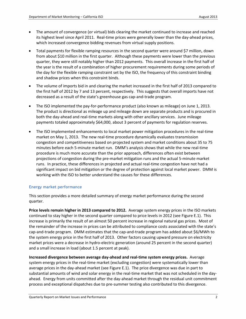
Figure E.3 Monthly average virtual bids offered and cleared
Continued convergence bidding designed to take advantage of congestion. Market participants can hedge (or speculate) on potential congestion between points within the ISO system by placing an equal amount of virtual demand and supply bids at different internal locations during the same hour. This type of offsetting virtual position at internal locations accounted for an average of about 1,420 MW per hour of virtual demand offset by over 1,420 MW of virtual supply at other locations in the second quarter, up from 1,240 MW in the first quarter. These offsetting bids represented over 68 percent of all cleared bids in the second quarter.
Increased net revenues associated with virtual supply positions. In total, convergence bidders were paid almost $14 million in net revenues in the second quarter, compared to about $3 million in net
2 See 137 FERC ¶ 61,157 (2011) accepting and temporarily suspending convergence bidding at the inter-ties subject to the
outcome of a technical conference and a further commission order. See 143 FERC ¶ 61,157 (2013) conditionally accepting elimination of inter-tie convergence bidding. In the May 2013 order, FERC indicated that the ISO should address within a year the issue of structural separation between the hour-ahead and real-time markets or explain why it has not done so before it reevaluates the efficiency of convergence bidding on inter-ties. More information can also be found under FERC docket number ER11-4580-000.
-6,000
-4,000
-2,000
0
2,000
4,000
6,000
Apr May Jun Jul Aug Sep Oct Nov Dec Jan Feb Mar Apr May Jun
2012 2013
Ave
rage
ho
url
y m
ega
wat
ts
Virtual supply (cleared) Virtual supply (offered) Virtual demand (cleared)
Virtual demand (offered) Net virtual (cleared)

Department of Market Monitoring – California ISO August 2013
Quarterly Report on Market Issues and Performance 6
losses in the first quarter. Virtual demand accounted for a loss of around -$18.5 million, while virtual supply generated net revenues of about $32.3 million. This trend reflects that during the second quarter virtual supply positions profited from day-ahead prices that were systematically higher than real-time prices.
Special issues
Effect of cap-and-trade on ISO markets. Resources in the ISO market became subject to the state’s greenhouse gas cap-and-trade program in January 2013. The greenhouse gas allowance cost, a measure of the opportunity cost of emitting one metric ton of greenhouse gas, has been stable in the second quarter, varying between $13.50/mtCO2e and $15/mtCO2e and averaging around $14.59/mtCO2e, slightly above the average value for the first quarter, $14.55/mtCO2e.3 DMM estimates that these greenhouse gas compliance costs have increased the average wholesale electricity price by about $6/MWh. This is highly consistent with the additional emissions costs for gas units typically setting prices in the ISO market. In addition, both cleared imports and import bid quantities increased in the first half of 2013 compared to the first half of 2012 by 7 and 13 percent, respectively. This suggests that imports have not decreased as a result of the program.
Implementation of the pay-for-performance (mileage) product. In June, the ISO implemented the pay-for-performance product, often referred to as mileage, to complement the existing frequency regulation markets. In the first month of operation, mileage was a small part of the regulation market settlement. Implementation of the program was fairly smooth, and June mileage payments totaled approximately $64,000, about 3 percent of payments for regulation reserves. The ISO has a benchmark of 50 percent accuracy that a resource must meet to continue to be a regulation resource. On average, the performance accuracy was 53 percent for mileage down and 40 percent for mileage up in June.
Enhancements to the real-time local market power mitigation procedure. The new local market power mitigation procedure dynamically evaluates competitiveness based on actual system and market conditions. One of the main enhancements was the improved mitigation trigger. DMM’s analysis shows that in June and early July, the mitigation run accurately predicted congestion on a constraint 49 percent of the time in the real-time market, while the prediction accuracy was 84 percent in the day-ahead market. Much of the prediction error in the real-time market was due to the differences in model inputs between the 15-minute real-time pre-dispatch mitigation run and the 5-minute market run. This is because the mitigation processes for the 15-minute real-time pre-dispatch run roughly 35 to 75 minutes before the 5-minute market runs. In practice, these differences in projected and actual real-time congestion have not had a significant impact on bid mitigation since only a very few resources have bids actually mitigated, due to very competitive bidding in the market. In addition, since the pre-market mitigation runs tend to project congestion more frequently than actual congestion that occurs in real time, the procedures provide a high degree of protection against local market power. DMM is working with the ISO to better understand the causes for the differences in projected versus actual real-time congestion.
3 mtCO2e stands for metric tons of carbon dioxide equivalent, a standard emissions measurement.

Department of Market Monitoring – California ISO August 2013
Quarterly Report on Market Issues and Performance 7
1 Market performance
This section highlights key performance indicators of the markets in the second quarter:
Systemically higher day-ahead prices than real-time prices, in both peak and off-peak hours.
High average hour-ahead prices that exceeded average real-time prices in all three months.
Decreased frequency of high real-time price spikes.
Increased frequency of negative real-time prices and over-generation.
Continued differences in congestion between the day-ahead and real-time markets.
Increased real-time imbalance costs from historically low levels, driven by higher congestion imbalance offset costs.
Increases in overall bid cost recovery payments due to increased levels of minimum online commitments and exceptional dispatches due to pre-summer testing.
1.1 Energy market performance
This section assesses the efficiency of the energy market based on an analysis of the system energy component of day-ahead, hour-ahead and real-time market prices. Price convergence between these markets may help promote efficient commitment of internal and external generating resources.
Average real-time price levels decreased compared to day-ahead and hour-ahead prices during the quarter. Figure 1.1 and Figure 1.2 show monthly system marginal energy prices for peak and off-peak periods, respectively.
On a monthly average basis, peak hour-ahead prices were about $6/MWh lower than day-ahead prices in April, but were higher in May and June by about $8/MWh. These higher values for the peak hours are a result of a relatively small number of hours (e.g., 30 to 40) with extremely high hour-ahead prices. When these prices are excluded, the results indicate a greater convergence between the day-ahead and hour-ahead prices. Off-peak hour-ahead prices were about $6/MWh lower than day-ahead for the entire period.
Average system prices in the 5-minute real-time market were lower than the day-ahead prices by about $5/MWh during peak and off-peak periods. Factors contributing to the price differences between the day-ahead and real-time markets are modeling differences between the day-ahead and real-time markets, decreased flexibility as a result of hydro-electric generation, and increased real-time generation from variable generation including wind and solar resources.
Average system prices in the 5-minute real-time market were less than the hour-ahead prices on average about $9/MWh in peak hours while the difference in off-peak hours was minimal. The largest average difference was $15/MWh and occurred during the peak hours in June.

Department of Market Monitoring – California ISO August 2013
Quarterly Report on Market Issues and Performance 8
Figure 1.1 Average monthly on-peak prices – system marginal energy price
Figure 1.2 Average monthly off-peak – system marginal energy price
$0
$10
$20
$30
$40
$50
$60
Apr May Jun Jul Aug Sep Oct Nov Dec Jan Feb Mar Apr May Jun
2012 2013
Pri
ce (
$/M
Wh
)
Day-ahead Hour-ahead Real-time
$0
$10
$20
$30
$40
$50
$60
Apr May Jun Jul Aug Sep Oct Nov Dec Jan Feb Mar Apr May Jun
2012 2013
Pri
ce (
$/M
Wh
)
Day-ahead Hour-ahead Real-time

Department of Market Monitoring – California ISO August 2013
Quarterly Report on Market Issues and Performance 9
Figure 1.1 and Figure 1.2 show price divergence among average day-ahead, hour-ahead and real-time prices during the second quarter. The systematic difference in the renewable energy schedules between the day-ahead and real-time markets is one of the factors contributing to the relatively low real-time prices. On average, real-time wind generation was 760 MW higher than day-ahead schedules, reaching above 2,000 MW in some hours. On average, real-time solar generation in peak hours was around 260 MW higher than the day-ahead schedules, reaching up to 900 MW in some hours.
Post day-ahead residual unit commitments and exceptional dispatch commitments also contributed to relatively low real-time prices. Energy from residual unit commitments averaged around 50 MW, reaching up to 250 MW in some hours.4 Energy from exceptional dispatch commitments averaged around 75 MW, reaching above 500 MW in some hours.
Figure 1.3 and Figure 1.4 further illustrate that systematic differences between prices remained in the second quarter. Figure 1.3 shows average hourly prices for the second quarter. Hour-ahead prices were considerably higher than day-ahead prices in eight hours, hours ending 14 through 21. The maximum price difference was nearly $54/MWh and the average for these hours was $27/MWh. Real-time prices were higher than hour-ahead prices in seven hours, averaging almost $2/MWh higher in these hours. Day-ahead prices exceeded real-time prices in 22 hours and in the 2 remaining hours the price difference was within $1/MWh. The average price difference was nearly $5/MWh in the hours where day-ahead prices exceeded real-time prices.
Figure 1.4 highlights the magnitude of price differences for all hours in the hour-ahead and real-time markets based on a simple average of price differences in these markets. Based on the simple average (green line), price divergence was consistently in a downward direction with negative $5/MWh for the quarter. In June, the negative price difference was greater than $9/MWh.
Also shown in Figure 1.4, the average absolute price difference between the hour-ahead and real-time markets (gold line) shows that the price trend was upward, with May experiencing the highest level of absolute price divergence since December 2012 at over $20/MWh.5 The absolute average price differences for the quarter were about $17/MWh, up from $12/MWh in the previous quarter.
4 More than half of the capacity committed by the residual unit commitment was from long-start units.
5 By taking the absolute value, the direction of the difference is eliminated and only the magnitude of the difference remains. Mathematically, this measure will always exceed the simple average of price differences shown in Figure 1.4 if both negative as well as positive price differences occur. If the magnitude decreases, price convergence would be improving. If the magnitude increases, price convergence would be getting worse. DMM does not anticipate that the average absolute price convergence should be zero. This metric is considered secondary to the simple average metrics and helps to further interpret price convergence.

Department of Market Monitoring – California ISO August 2013
Quarterly Report on Market Issues and Performance 10
Figure 1.3 Hourly comparison of system marginal energy prices (April – June)
Figure 1.4 Difference in monthly hour-ahead and real-time prices based on simple average and absolute average of price differences (system marginal energy, all hours)
$0
$20
$40
$60
$80
$100
$120
1 2 3 4 5 6 7 8 9 10 11 12 13 14 15 16 17 18 19 20 21 22 23 24
Pri
ce (
$/M
Wh
)
Day-ahead Hour-ahead Real-time
-$10
-$5
$0
$5
$10
$15
$20
$25
Apr May Jun Jul Aug Sep Oct Nov Dec Jan Feb Mar Apr May Jun
2012 2013
Pri
ce (
$/M
Wh
)
Average of real-time price minus hour-ahead priceAverage of absolute real-time price minus hour-ahead price

Department of Market Monitoring – California ISO August 2013
Quarterly Report on Market Issues and Performance 11
1.2 Real-time price variability
Real-time market prices historically have been very variable, which is highlighted in this section along with reasons why the variability occurs.
Figure 1.5 shows on average a slight decrease in the frequency of price spikes that occur in each investor-owned utility area in the real-time market in the second quarter, from an average of 0.7 percent in the first quarter to about 0.6 percent in the second quarter. A dramatic reduction in the frequency of all categories of real-time price spikes occurred in June, with an average of only 0.1 percent of all intervals with price spikes.
As in the previous two quarters, the ISO continued to increase the flexible ramping constraint requirements during the evening ramping hours. Also, the ISO implemented an enhancement in December 2012 that limits the ability of load adjustments made by the ISO operators to create market infeasibilities. Following the trend of the first quarter, the total frequency of price spikes was downward, with the exception of price spikes within the $250/MWh to $500/MWh category in May. The greatest portion of the price spikes in this category were related to congestion on SCE_PCT_IMP_BG, 7820_TL 230S_OVERLOAD_NG and PATH15_BG.
Figure 1.5 Frequency of price spikes (all LAP areas)
The number of power balance constraint relaxation intervals resulting from insufficient upward ramping capacity decreased significantly in the second quarter compared to the previous quarter, as seen in Figure 1.6. This decrease is likely related to the increased procurement of ramping capacity associated with the flexible ramping constraint. Unlike previous quarters, extreme congestion played only a minor role in instances of insufficient upward ramping in the second quarter.
0.0%
0.2%
0.4%
0.6%
0.8%
1.0%
1.2%
1.4%
1.6%
1.8%
Apr May Jun Jul Aug Sep Oct Nov Dec Jan Feb Mar Apr May Jun
2012 2013
Pe
rce
nt
of
real
-tim
e in
terv
als
$250 to $500 $500 to $750 $750 to $1000 $1000 to LMP

Department of Market Monitoring – California ISO August 2013
Quarterly Report on Market Issues and Performance 12
Power balance relaxations can occur in the presence of congestion. In the second quarter, around 30 percent of the upward ramping capacity relaxations shown in Figure 1.6 resulted from extreme regional congestion, compared to about 60 percent in the first quarter. Sometimes extreme congestion on constraints within the ISO system can limit the availability of significant amounts of supply. This can cause system-wide limitations in upward ramping capacity, and thus cause relaxations in the power balance constraint. In these cases, the cost of relaxing the system power balance constraint is less expensive than the cost of relaxing the internal constraint. Therefore, the system power balance constraint is relaxed to deal with upward ramping limitations in the congested portion of the ISO system.6
There was an increase in the number of real-time power balance constraint relaxations from insufficiencies of dispatchable decremental energy in the second quarter relative to the first quarter, as shown in Figure 1.7.7 Increased real-time generation from variable resources, seasonal increases in hydro-electric generation and low shoulder period loads increased the number of instances where insufficient downward ramping capacity was available in the market compared to the previous quarter. Almost all of these constraint relaxations resulted from system-wide over-generation conditions.
Figure 1.6 Relaxation of power balance constraint because of insufficient upward ramping capacity
6 This is primarily true for large regional constraints. For very small local constraints, the opposite is true. In the case of local constraints, the cost of relaxing the local constraint is less expensive than the cost of relaxing the system power balance constraint. Thus, the local constraint is relaxed instead of the power balance constraint.
7 When these downward ramping limitations occur, the real-time system energy price is set by a penalty parameter equal to -$35/MWh, just below the bid floor of -$30/MWh.
0.0%
0.5%
1.0%
1.5%
2.0%
0
50
100
150
200
Apr May Jun Jul Aug Sep Oct Nov Dec Jan Feb Mar Apr May Jun
2012 2013
Pe
rce
nt
of
inte
rval
s
Co
un
t o
f in
terv
als
Insufficient upward ramping capacity due to transmission constraint
Insufficient upward ramping capacity due to system energy shortage
Percent of intervals with insufficient upward ramping capacity

Department of Market Monitoring – California ISO August 2013
Quarterly Report on Market Issues and Performance 13
Figure 1.7 Relaxation of power balance constraint because of insufficient downward ramping capacity
Figure 1.8 Factors causing high real-time prices
0%
1%
2%
3%
4%
0
100
200
300
400
Apr May Jun Jul Aug Sep Oct Nov Dec Jan Feb Mar Apr May Jun
2012 2013
Pe
rce
nt
of
inte
rval
s
Co
un
t o
f in
terv
als
5-minute intervals with insufficient downward ramping capacity
Percent of intervals with insufficient downward ramping capacity
0.0%
0.5%
1.0%
1.5%
Apr May Jun Jul Aug Sep Oct Nov Dec Jan Feb Mar Apr May Jun
2012 2013
Inte
rval
s w
ith
pir
ce n
ear
or
abo
ve b
id c
ap
System power balance constraint Power balance and congestion
Congestion High priced bid
Other

Department of Market Monitoring – California ISO August 2013
Quarterly Report on Market Issues and Performance 14
Around 73 percent of high real-time prices were caused by congestion or a combination of power balance constraint relaxations and congestion in the second quarter. About 57 percent of these instances can be attributed to congestion alone, while about 21 percent were a result of system-wide power balance relaxations. High priced bids resulted in only 5 percent of the high prices. Figure 1.8 highlights the different factors driving high real-time prices at a regional level. The prices in this figure include all intervals in which the real-time price for a load aggregation point was approaching the bid cap.8
1.3 Congestion
Congestion within the ISO system in the second quarter affected overall prices less in the day-ahead and real-time markets than in the first quarter. However, congestion continued to have a significant impact on the market, particularly into the Southern California Edison area. Much of the congestion was related to adjustments of the flows on the SCE percent import branch group constraint (SCE_PCT_IMP_BG), outages and retirement of San Onofre Nuclear Generating Station (SONGS) units 2 and 3, and other generation and transmission events.
The impact of congestion on any constraint on each pricing node in the ISO system can be calculated by summing the product of the shadow price of that constraint and the shift factor for that node relative to the congested constraint. This calculation can be done for individual nodes, as well as groups of nodes that represent different load aggregation points or local capacity areas.
Often, congestion on constraints in Southern California increases prices within the Southern California Edison and San Diego Gas and Electric areas, but decreases prices in the Pacific Gas and Electric area. This is the inverse of congestion in Northern California. The price impacts on individual constraints can differ between the day-ahead and real-time markets, as seen in the following sections.
1.3.1 Congestion impacts of individual constraints
Day-ahead congestion
Congestion in the day-ahead market generally occurred more frequently than the real-time market. Table 1.1 provides information related to the frequency and magnitude of day-ahead market congestion.
The most congested constraint in the ISO system was the constraint limiting imports into the SCE area (SCE_PCT_IMP_BG). This constraint was congested in about 51 percent of the hours in the second quarter, down from 71 percent in the previous quarter. When congestion occurred on this constraint, prices in the SCE area increased about $4.29/MWh and decreased for SDG&E and PG&E areas about $3.65/MWh. This constraint was directly affected by the SONGS outages and retirement.
The second most congested constraint in the SCE area was the BARRE-LEWIS_NG. This constraint increased prices in the SCE and SDG&E areas by $1.29/MWh and $0.91/MWh respectively, while decreasing prices in the PG&E area by $1.06/MWh. This constraint was also directly affected by the SONGS outages and retirement.
8 The analysis behind this figure reviews price spikes above $700/MWh.

Department of Market Monitoring – California ISO August 2013
Quarterly Report on Market Issues and Performance 15
The San Diego area had the greatest instances of significant congestion. Many of these constraints were related to the Barre-Lewis nomogram which protects the Barre-Lewis 220 kV line for a contingency on the Barre-VillaPark 220 kV line and the Serrano transformer flowgate which protects the Serrano 500/220 kV transformer for a contingency on the parallel transformer. In addition, the 7820_TL 230S_OVERLOAD_NG constraint, which protects the Imperial Valley-El Centro 230 kV line for a loss of the Imperial Valley-North Gila 500 kV line, was binding in almost 14 percent of the hours. It increased prices in the SDG&E area by $7.69/MWh, while it decreased prices in the PG&E area by $1.01/MWh.
In the PG&E area, the most congested constraint was the Path 15 branch group (Path15_BG). This constraint occurred mainly due to forced outages, planned maintenance, variable resource deviation and unscheduled flows on the California-Oregon Intertie (COI). Congestion on this branch group occurred in nearly 10 percent of hours in the south-to-north direction. During these hours, prices in the PG&E area increased by about $1.60/MWh and prices in the SCE and SDG&E areas decreased by about $1.32/MWh.
Table 1.1 Impact of congestion on day-ahead prices by load aggregation point in congested hours
Area Constraint Q1 Q2 PG&E SCE SDG&E PG&E SCE SDG&E
PG&E PATH15_BG 7.7% 9.8% $1.68 -$1.43 -$1.43 $1.60 -$1.32 -$1.32
30875_MC CALL _230_30880_HENTAP2 _230_BR_1 _1 1.9% $0.57 -$0.45 -$0.45
30735_METCALF _230_30042_METCALF _500_XF_13 1.3% $2.26 -$1.92 -$1.92
LOSBANOSNORTH_BG 1.2% $2.74 -$2.09 -$2.09
SCE SCE_PCT_IMP_BG 71.2% 51.2% -$3.93 $4.85 -$3.89 -$3.66 $4.29 -$3.63
BARRE-LEWIS_NG 23.9% 5.3% -$1.32 $1.84 $0.21 -$1.06 $1.29 $0.91
PATH26_BG 1.1% -$1.83 $1.47 $1.47
SLIC 2088287_BARRE-LEWIS_NG 0.7% -$1.28 $2.13
SDG&E 7820_TL 230S_OVERLOAD_NG 13.6% -$1.01 $7.69
22768_SOUTHBAY_69.0_22604_OTAY _69.0_BR_2 _1 5.5% $0.96
SOUTHLUGO_RV_BG 0.4% 3.3% -$3.24 $2.47 $4.42 -$5.15 $3.56 $5.43
SDGE_PCT_UF_IMP_BG 2.2% -$0.76 -$0.76 $7.58
24016_BARRE _230_24044_ELLIS _230_BR_1 _1 1.7% -$2.46 -$0.67 $15.70
SLIC 2122013 BARRE-ELLIS-230S_NG 1.6% -$0.46 $4.91
24016_BARRE _230_24044_ELLIS _230_BR_4 _1 1.6% -$0.45 $2.17
7830_SXCYN_CHILLS_NG 0.1% 1.3% $0.56 $9.51
24138_SERRANO _500_24137_SERRANO _230_XF_2 _P 0.9% -$3.53 $1.88 $7.28
24138_SERRANO _500_24137_SERRANO _230_XF_1 _P 0.8% -$3.02 $1.67 $6.02
24016_BARRE _230_24044_ELLIS _230_BR_3 _1 0.7% -$0.47 $2.34
SLIC 2077347 TL50003_NG 0.6% $6.05
SLIC 2067610 TL50001_NG 0.6% $12.23
SLIC 2122013 Barre-Ellis DLO 0.6% -$2.54 $15.20
SLIC 2111709_IV500North_BUS_NG 0.5% $20.93
SLIC 2122013 Barre-Ellis DLO_20 0.4% -$1.97 $12.42
22192_DOUBLTTP_138_22300_FRIARS _138_BR_1 _1 3.4% 0.2% $4.27 $6.81
IVALLYBANK_XFBG 2.6% $0.84
SLIC 2051445 TL23050_NG 2.3% $6.31
SLIC 2090466 and 2090467 SOL 2.3% $15.29
SLIC 2112931 EL CENTRO BK1_NG 1.2% $5.05
MIGUEL_BKs_MXFLW_NG 0.4% -$1.04 $11.65
24138_SERRANO _500_24137_SERRANO _230_XF_3 0.4% -$17.48 $41.61
SLIC 2094078 IV Bank81_NG 0.2% -$3.54 $24.91
Q1Frequency Q2

Department of Market Monitoring – California ISO August 2013
Quarterly Report on Market Issues and Performance 16
As shown in Table 1.1, congestion on other constraints significantly affected prices during hours when congestion occurred. However, with the exception of the SCE_PCT_IMP_BG, the 7820_TL 230S_OVERLOAD_NG and the PATH15_BG, internal congestion occurred infrequently, and typically had a minimal impact on overall day-ahead energy prices.
Real-time congestion
Congestion in the real-time market differs from the day-ahead market in that real-time congestion occurs less frequently overall, but often with a larger price effect in the intervals when it occurs. Table 1.2 shows the frequency and magnitude of congestion in the fourth quarter.
Three out of the top five most frequently congested constraints in the first quarter were in the PG&E area. The most frequently congested constraint, PATH15_S-N, was binding in 4.5 percent of all intervals. This constraint increased prices by about $17.53/MWh in the PG&E area and decreased prices in SCE and SDG&E areas by $14.29/MWh. This constraint was influenced by maintenance outages on the Los Banos – Gates (500 kV) and Midway - Los Banos (500 kV) lines, variable resources and unscheduled flows on COI.
The second most congested constraint in the quarter was in the San Diego area, the 7820_TL 230S_OVERLOAD_NG, with congestion in nearly 3 percent of the hours. This constraint alone increased the prices in the SDG&E area by $34.48/MWh in congested hours, while prices in the PG&E area decreased by about $1.75/MWh. This constraint protects the Imperial Valley-El Centro 230 kV line for a loss of the Imperial Valley-North Gila 500 kV line in the north-to-south direction.9
Prices in the San Diego area were affected by multiple constraints. A few Barre-Lewis nomograms drove the prices in the SDG&E area up by about $20/MWh, while decreasing the PG&E and SCE prices by $3/MWh and $1/MWh, respectively. The other remaining constraints in the SDG&E area were binding in less than 0.5 percent of the intervals, but had significant price impact on the SDG&E area prices when they were binding. These constraints include the Serrano transformer, the Sycamore-Canyon and the Hoodoo-Wash nomograms, and the South of Lugo and SCIT branch groups.
Southern California Edison prices were most influenced by the SCE_PCT_IMP_BG (about 2 percent of intervals). This constraint increased prices in the SCE area by about $58/MWh and decreased both the PG&E and SDG&E area prices by nearly $48/MWh. Congestion on the SCE_PCT_IMP_BG was directly affected by the SONGS outages and retirement, variable resource output, generation outages and derates.
9 Prior to summer 2013, the Hoodoowash-North Gila 500 kV line flowgate was congested frequently due to heavy east-to-west flows into the Pacific Southwest. Following infrastructure improvements, congestion on the Hoodoowash-North Gila constraint was reduced significantly and the 7820_TL 230S_OVERLOAD_NG became the next binding constraint.

Department of Market Monitoring – California ISO August 2013
Quarterly Report on Market Issues and Performance 17
Table 1.2 Impact of congestion on real-time prices by load aggregation point in congested intervals
Overall, congestion occurred more frequently in the day-ahead market compared to the real-time market, as shown by a comparison of Table 1.1 and Table 1.2. However, in general, when congestion occurs, its impact on prices is larger in the real-time market than the day-ahead market. Differences in congestion in the day-ahead and real-time markets occur as system conditions change, as virtual bids liquidate, and as constraints are sometimes adjusted in real-time to make market flows consistent with actual flows and to provide a reliability margin.
For instance, the SCE_PCT_IMP_BG was binding in roughly 51 percent of the hours in the day-ahead market compared to around 2 percent of intervals in the real-time market. While this constraint increased day-ahead prices in the SCE area by nearly $4/MWh, it increased prices by over $58/MWh in the real-time market. A similar pattern can also be seen with the 7820_TL 230S_OVERLOAD_NG constraint.
Area Constraint Q1 Q2 PG&E SCE SDG&E PG&E SCE SDG&E
PG&E PATH15_S-N 2.1% 4.5% $52.05 -$43.98 -$43.98 $17.53 -$14.29 -$14.29
TRACY500_BG 2.3% -$9.51 $7.42 $7.42
30735_METCALF _230_30042_METCALF _500_XF_13 2.2% $29.35 -$31.17 -$31.17
6110_TM_BNK_FLO_TMS_DLO_NG 1.2% $7.51 -$3.80 -$3.80
LBN_S-N 0.9% $28.13 -$23.22 -$23.22
30735_METCALF _230_30750_MOSSLD _230_BR_1 _1 0.6% $23.95 -$23.75 -$23.75
30055_GATES1 _500_30900_GATES _230_XF_11_P 0.2% $7.58 -$6.64 -$6.64
T-135 VICTVLUGO_PVDV_NG 0.1% 0.0% $33.40 -$38.73 $1.06 -$1.57
SCE SCE_PCT_IMP_BG 10.0% 2.2% -$33.78 $41.04 -$33.48 -$47.91 $58.30 -$47.41
PATH26_N-S 2.0% 1.2% -$23.96 $19.63 $19.63 -$72.06 $58.65 $58.65
24155_VINCENT _230_24091_MESA CAL_230_BR_1 _1 0.4% -$11.16 $9.31 $8.74
BARRE-LEWIS_NG 5.4% 0.2% -$8.62 $5.60 -$6.64 -$5.70 $5.30 $1.97
PATH15_N-S 0.0% -$56.37 $47.06 $47.06
SDG&E 7820_TL 230S_OVERLOAD_NG 0.4% 2.6% $29.90 -$1.75 $34.48
SLIC 2122013 Barre-Ellis DLO_16 0.6% -$3.44 -$0.90 $23.02
SLIC 2122013 Barre-Ellis DLO_17 0.6% -$4.49 -$1.25 $29.85
SLIC 2122013 Barre-Ellis DLO_21 0.5% -$2.20 $14.49
SLIC 2077347 TL50003_NG 0.5% $0.83 $54.19
SOUTH_OF_LUGO 0.4% -$20.66 $16.05 $22.56
24138_SERRANO _500_24137_SERRANO _230_XF_2 _P 0.1% 0.4% -$37.04 $92.29 -$23.63 $14.79 $51.60
24016_BARRE _230_24044_ELLIS _230_BR_1 _1 0.4% -$1.52 -$0.55 $9.86
7830_SXCYN_CHILLS_NG 0.3% $19.99
SOUTHLUGO_RV_BG 0.0% 0.2% -$2.45 $1.74 $3.24 -$157.14 $110.45 $160.42
22342_HDWSH _500_22536_N.GILA _500_BR_1 _1 0.2% -$8.74 $55.06
SLIC 2126995 SONGS_NG1 0.1% -$47.35 $441.78
SDGE_PCT_UF_IMP_BG 0.1% -$13.32 -$13.32 $141.64
30060_MIDWAY _500_24156_VINCENT _500_BR_2 _2 0.0% 0.0% -$320.31 $267.35 $267.35 -$0.84 $0.72 $0.73
IVALLYBANK_XFBG 3.1% $2.55
7830_TL 230S_IV-SX-OUT_NG 0.5% $51.47
22464_MIGUEL _230_22468_MIGUEL _500_XF_81 0.4% -$2.22 -$5.25 $15.46
SLIC 2090466 and 2090467 SOL 0.3% $30.74
SLIC 2051445 TL23050_NG 0.2% $46.55
SLIC 2112931 EL CENTRO BK1_NG 0.2% $49.40
24138_SERRANO _500_24137_SERRANO _230_XF_3 0.1% -$32.00 $80.19
Frequency Q1 Q2

Department of Market Monitoring – California ISO August 2013
Quarterly Report on Market Issues and Performance 18
1.3.2 Congestion impact on average prices
This section provides an assessment of differences on overall average prices in the day-ahead and real-time markets caused by congestion between different areas of the ISO system. Unlike the analysis provided in the previous section, this assessment is made based on the average congestion component of the price as a percent of the total price during all congested and non-congested hours. This approach shows the impact of congestion taking into account the frequency that congestion occurs as well as the magnitude of the impact that congestion has when it occurs.10 The price impact of congestion in all hours in the second quarter was larger in the day-ahead market than the real-time market.11
Day-ahead price impacts
Table 1.3 shows the overall impact of day-ahead congestion on average prices in each load area in the second quarter by constraint.
The SCE_PCT_IMP_BG increased day-ahead prices in the SCE area above system average prices by $2.20/MWh or 4.8 percent, down from $3.45/MWh (7.5 percent) in the previous quarter. Prices decreased by about $1.86/MWh (4.5 percent) in PG&E and SDG&E areas. This constraint is designed to ensure that enough generation is available to balance demand from units within the SCE area in the event of a severe under-frequency event that would result in the SCE area being separated from the rest of the interconnection.
In the SDG&E area, the 7820_TL 230S_OVERLOAD_NG increased prices by $1.05/MWh or 2.3 percent and decreased PG&E area prices by $0.03/MWh or 0.06 percent with no significant price impact on SCE area prices.
The day-ahead prices in the PG&E area were driven by the PATH15_BG, which increased prices by $0.16/MWh or around 0.37 percent. This was associated with a planned outage on the Los Banos – Gates and Midway - Los Banos 500 kV lines.
The overall impact of congestion on day-ahead prices in the PG&E area decreased prices by about $2.07/MWh or about 4.9 percent from the system average. This occurred because prices in the PG&E area were lower when congestion occurred on the constraints limiting flows into the SCE and SDG&E areas.
10
In addition, this approach identifies price differences caused by congestion without including price differences that result from variations in transmission losses at different locations.
11 As mentioned before, congestion in the real-time market often has a larger price effect in intervals when it occurs. However, the overall price impact of congestion depends on the frequency of congestion along with the magnitude of the price effect.

Department of Market Monitoring – California ISO August 2013
Quarterly Report on Market Issues and Performance 19
Table 1.3 Impact of congestion on overall day-ahead prices
Real-time price impacts
Table 1.4 shows the overall impact of real-time congestion on average prices in each load area in the second quarter by constraint.
Congestion drove prices in the SCE area above system average prices by about $1.04/MWh or 2.7 percent. Most of this increase was due to limits on the percentage of load in the SCE area that can be met by total flows on all transmission paths into the SCE area (SCE_PCT_IMP_BG). Another major driver of congestion was the Path 26 N-S constraint, which increased prices in the SCE area by $0.68/MWh (1.75 percent).
Prices in the San Diego area were impacted the most by congestion associated with the SCE_PCT_IMP_BG, PATH15_S-N and PATH26_N-S constraints. The SCE_PCT_IMP_BG and PATH15_S-N constraints drove SDG&E prices down while PATH26_N-S drove prices up. These three constraints drove San Diego area prices below the system average by nearly 2.5 percent or about $1/MWh.
The overall impact of congestion on prices in the PG&E area was to decrease prices from the system average by about $0.71/MWh or about 2 percent. Prices in the PG&E area are lowered when congestion occurs on the constraints that limit flows in the north-to-south direction (e.g., PATH26_N-S) and on constraints limiting flows into the SCE (e.g., SCE_PCT_IMP_BG) and SDG&E areas. Congestion on the Path15_S-N constraint was influenced by the Los Banos – Gates and Midway – Los Banos 500 kV line outages, compensating injections, variable resources and flows on the California-Oregon Inter-tie (COI). This constraint increased prices by $0.78/MWh (2 percent) during the first quarter in the PG&E area.
Constraint $/MWh Percent $/MWh Percent $/MWh Percent
SCE_PCT_IMP_BG -$1.88 -4.47% $2.20 4.82% -$1.86 -4.14%
7820_TL 230S_OVERLOAD_NG -$0.03 -0.06% $1.05 2.34%
SOUTHLUGO_RV_BG -$0.17 -0.41% $0.12 0.26% $0.18 0.41%
PATH15_BG $0.16 0.37% -$0.13 -0.28% -$0.13 -0.29%
24016_BARRE _230_24044_ELLIS _230_BR_1 _1 -$0.04 -0.10% -$0.01 -0.02% $0.27 0.59%
SDGE_PCT_UF_IMP_BG -$0.02 -0.04% -$0.02 -0.04% $0.17 0.37%
BARRE-LEWIS_NG -$0.06 -0.14% $0.07 0.15% $0.00 0.01%
7830_SXCYN_CHILLS_NG $0.13 0.28%
24138_SERRANO _500_24137_SERRANO _230_XF_2 _P -$0.03 -0.07% $0.02 0.04% $0.06 0.14%
SLIC 2122013 Barre-El l i s DLO -$0.02 -0.04% $0.09 0.20%
SLIC 2111709_IV500North_BUS_NG $0.10 0.21%
24138_SERRANO _500_24137_SERRANO _230_XF_1 _P -$0.03 -0.06% $0.01 0.03% $0.05 0.11%
SLIC 2122013 BARRE-ELLIS-230S_NG -$0.01 -0.02% $0.08 0.18%
LOSBANOSNORTH_BG $0.03 0.08% -$0.03 -0.06% -$0.03 -0.06%
30735_METCALF _230_30042_METCALF _500_XF_13 $0.03 0.07% -$0.03 -0.05% -$0.03 -0.06%
SLIC 2067610 TL50001_NG $0.07 0.16%
22768_SOUTHBAY_69.0_22604_OTAY _69.0_BR_2 _1 $0.05 0.12%
SLIC 2122013 Barre-El l i s DLO_20 -$0.01 -0.02% $0.05 0.10%
24016_BARRE _230_24044_ELLIS _230_BR_4 _1 -$0.01 -0.02% $0.03 0.08%
SLIC 2077347 TL50003_NG $0.04 0.09%
30875_MC CALL _230_30880_HENTAP2 _230_BR_1 _1 $0.01 0.03% -$0.01 -0.02% -$0.01 -0.02%
Other -$0.02 -0.04% -$0.01 -0.03% $0.06 0.14%
Total -$2.07 -4.9% $2.19 4.8% $0.43 1.0%
PG&E SCE SDG&E

Department of Market Monitoring – California ISO August 2013
Quarterly Report on Market Issues and Performance 20
Table 1.4 Impact of congestion on overall real-time prices
Overall, real-time congestion occurred less frequently than day-ahead congestion. In contrast to the first quarter, its overall price impact was smaller than what occurred in the day-ahead market. As mentioned earlier, the differences in congestion can be attributed to differences in market conditions as well as changes associated with conforming line limits to make market flows reflect actual flows as well as to provide a reliability margin.
Congestion price difference between the day-ahead, hour-ahead and real-time markets
This section compares the congestion price differences between the day-ahead, hour-ahead and real-time markets as a simple and absolute average over time. In terms of both the simple and absolute averages, congestion differences have reduced somewhat between the day-ahead and real-time markets in the second quarter compared to the previous quarter, as the frequency and impact of
Constraint $/MWh Percent $/MWh Percent $/MWh Percent
SCE_PCT_IMP_BG -$1.03 -2.75% $1.25 3.22% -$1.02 -2.58%
PATH26_N-S -$0.84 -2.24% $0.68 1.75% $0.68 1.72%
PATH15_S-N $0.78 2.08% -$0.64 -1.63% -$0.64 -1.61%
30735_METCALF _230_30042_METCALF _500_XF_13 $0.64 1.70% -$0.68 -1.74% -$0.68 -1.71%
SOUTHLUGO_RV_BG -$0.36 -0.96% $0.25 0.65% $0.37 0.93%
7820_TL 230S_OVERLOAD_NG $0.00 0.00% $0.88 2.23%
LBN_S-N $0.26 0.69% -$0.21 -0.55% -$0.21 -0.54%
TRACY500_BG -$0.22 -0.59% $0.17 0.44% $0.17 0.43%
30735_METCALF _230_30750_MOSSLD _230_BR_1 _1 $0.13 0.35% -$0.13 -0.34% -$0.13 -0.33%
SLIC 2126995 SONGS_NG1 -$0.04 -0.10% $0.35 0.89%
24138_SERRANO _500_24137_SERRANO _230_XF_2 _P -$0.09 -0.25% $0.06 0.15% $0.21 0.52%
SLIC 2077347 TL50003_NG $0.00 0.00% $0.26 0.66%
SOUTH_OF_LUGO -$0.09 -0.24% $0.07 0.18% $0.10 0.25%
SLIC 2122013 Barre-Ellis DLO_17 -$0.03 -0.07% -$0.01 -0.01% $0.18 0.45%
SLIC 2122013 Barre-Ellis DLO_16 -$0.02 -0.06% $0.00 -0.01% $0.14 0.37%
6110_TM_BNK_FLO_TMS_DLO_NG $0.09 0.24% -$0.02 -0.04% -$0.02 -0.04%
22342_HDWSH _500_22536_N.GILA _500_BR_1 _1 -$0.02 -0.04% $0.11 0.27%
24155_VINCENT _230_24091_MESA CAL_230_BR_1 _1 -$0.04 -0.12% $0.04 0.10% $0.04 0.09%
SCIT_BG -$0.04 -0.10% $0.04 0.09% $0.04 0.10%
SDGE_PCT_UF_IMP_BG -$0.01 -0.02% -$0.01 -0.02% $0.08 0.19%
SLIC 2122013 Barre-Ellis DLO_21 -$0.01 -0.03% $0.07 0.18%
7830_SXCYN_CHILLS_NG $0.06 0.14%
24016_BARRE _230_24044_ELLIS _230_BR_1 _1 -$0.01 -0.02% $0.00 -0.01% $0.04 0.10%
30055_GATES1 _500_30900_GATES _230_XF_11_P $0.02 0.04% -$0.01 -0.03% -$0.01 -0.03%
30735_METCALF _230_30042_METCALF _500_XF_12 $0.01 0.03% -$0.01 -0.03% -$0.01 -0.03%
SLIC 2122013 Barre-Ellis DLO_19 $0.00 -0.01% $0.03 0.08%
30875_MC CALL _230_30880_HENTAP2 _230_BR_1 _1 $0.01 0.03% -$0.01 -0.03% -$0.01 -0.03%
SLIC 2127305_PVDV-ELDLG_NG $0.01 0.03% -$0.02 -0.06%
24016_BARRE _230_24044_ELLIS _230_BR_3 _1 $0.00 -0.01% $0.02 0.05%
POTRERO_MSL -$0.01 -0.02% $0.01 0.02% -$0.01 -0.02%
BARRE-LEWIS_NG -$0.01 -0.03% $0.01 0.02% $0.00 0.00%
Other $0.21 0.57% $0.19 0.49% $0.10 0.26%
Total -$0.71 -1.9% $1.04 2.7% $1.16 2.9%
PG&E SCE SDG&E

Department of Market Monitoring – California ISO August 2013
Quarterly Report on Market Issues and Performance 21
congestion decreased. However, congestion differences increased between day-ahead and hour-ahead markets as hour-ahead prices increased significantly during peak hours in the second quarter.
Figure 1.9 shows the monthly average and absolute congestion price differences between the day-ahead and real-time markets since April 2011 for each load area. Figure 1.10 shows the monthly average and absolute congestion price difference between the day-ahead and hour-ahead markets by load area for the same period.
With the exception of SDG&E congestion in early 2011, which had short periods of congestion differences, the simple average (dashed line) and absolute average (solid line) price divergence between the day-ahead and the other markets was relatively small in 2011. This trend continued into the first part of 2012. However, beginning in February 2012 and continuing through the rest of the year, day-ahead market congestion differed significantly from both real-time and hour-ahead congestion with the simple average and even more so with the absolute average. Except for April, in 2013 the San Diego area congestion has, in absolute terms, moved in-line with the other areas. This is primarily due to the nature of the congestion in the second quarter, which was mostly impacted by the SCE_PCT_IMP_BG constraint and less so by constraints specific to San Diego.
As shown in Figure 1.9, in April 2013 the absolute difference in load area prices between the day-ahead market and the real-time market was around $9/MWh while the average difference was within a couple dollars. Figure 1.10 shows day-ahead and hour-ahead market price differences between the load areas increased in absolute terms. The average difference was positive in the SCE area, but negative in SDG&E and PG&E areas. In June 2013, these load area price differences for the SCE area averaged about $11/MWh, while they were -$5/MWh for the SDG&E and PG&E areas.
Figure 1.9 Monthly average and absolute congestion price differences between the day-ahead and real-time markets
-$10
$0
$10
$20
$30
$40
Ap
r
May Jun
Jul
Au
g
Sep
Oct
No
v
De
c
Jan
Feb
Mar
Ap
r
May Jun
Jul
Au
g
Sep
Oct
No
v
De
c
Jan
Feb
Mar
Ap
r
May Jun
2011 2012 2013
Pri
ce (
$/M
Wh
)
Average absolute real-time congestion price minus day-ahead price - SDG&E
Average absolute real-time congestion price minus day-ahead price - PG&E
Average absolute real-time congestion price minus day-ahead price - SCE
Average real-time congestion price minus day-ahead price - SDG&E
Average real-time congestion price minus day-ahead price - PG&E
Average real-time congestion price minus day-ahead price - SCE

Department of Market Monitoring – California ISO August 2013
Quarterly Report on Market Issues and Performance 22
Figure 1.10 Monthly average and absolute congestion price differences between the day-ahead and hour-ahead markets
1.4 Real-time imbalance offset costs
Real-time imbalance offset costs totaled about $56 million in the second quarter, an increase over the historically low value of $21 million in the first quarter. This was also slightly above the average quarterly offset cost for 2011 and 2012 of about $50 million. Congestion offset costs accounted for approximately 70 percent of the total imbalance costs during this quarter, totaling about $41 million. The remaining $15 million were incurred through energy imbalance offset costs, which remained relatively consistent with previous periods.
High real-time congestion offset costs on six days were due to loop flows and forced outages, including wildfires. Other special system conditions account for 35 percent of total real-time imbalance offset costs.12 In contrast, much of the congestion related uplift costs in the summer and fall of 2012 were related to more systematic and predictable congestion patterns stemming from unscheduled flows and market modeling differences. In part, the ISO’s efforts to address systematic modeling differences between the day-ahead and real-time markets, including better alignment of day-ahead and real-time transmission limits and modification of the constraint relaxation parameter, contributed to reducing real-time imbalance costs compared to the summer of 2012. Even so, the possibility of high real-time imbalance offset costs continues to exist.
12
This includes a day in late June when the congestion offset cost was notably high during periods of operator adjustments to the load in the hour-ahead market.
-$10
$0
$10
$20
$30
$40
Ap
r
May Jun
Jul
Au
g
Sep
Oct
No
v
De
c
Jan
Feb
Mar
Ap
r
May Jun
Jul
Au
g
Sep
Oct
No
v
De
c
Jan
Feb
Mar
Ap
r
May Jun
2011 2012 2013
Pri
ce (
$/M
Wh
)
Average absolute hour-ahead congestion price minus day-ahead price - SDG&E
Average absolute hour-ahead congestion price minus day-ahead price - PG&E
Average absolute hour-ahead congestion price minus day-ahead price - SCE
Average hour-ahead congestion price minus day-ahead price - SDG&E
Average hour-ahead congestion price minus day-ahead price - PG&E
Average hour-ahead congestion price minus day-ahead price - SCE

Department of Market Monitoring – California ISO August 2013
Quarterly Report on Market Issues and Performance 23
Figure 1.11 Real-time imbalance offset costs
1.5 Bid cost recovery payments
Bid cost recovery payments are designed to ensure that generators receive enough market revenues to cover the cost of all their bids when dispatched by the ISO.13 Bid cost recovery payments totaled around $33 million in the second quarter, compared to $21 million in the first quarter (see Figure 1.12 for a monthly breakdown).
Increases in minimum online commitments and exceptional dispatch commitments for summer testing and other reasons caused higher day-ahead and real-time bid cost recovery payments, totaling around $26 million. The real-time portion of bid cost recovery payments was significantly higher in the second quarter, reaching around $15 million. Around half of the real-time commitment costs resulted from unit commitments through exceptional dispatches due to pre-summer testing.
The month of May experienced much higher day-ahead bid cost recovery payments than the previous months, about $7 million. These payments can be attributed to minimum online commitments and unit testing for the summer during this period.14
13
Bid cost recovery covers the bids for start-up, minimum load, ancillary services, residual unit commitment availability, and day-ahead and real-time energy.
14 Some of the payments related to commitment costs due to unit testing may be subject to adjustment based on tariff clarification.
-$10
$0
$10
$20
$30
$40
$50
$60
$70
Apr May Jun Jul Aug Sep Oct Nov Dec Jan Feb Mar Apr May Jun
2012 2013
Tota
l co
st (
$ m
illio
ns)
Real-time congestion imbalance offset cost
Real-time energy imbalance offset cost

Department of Market Monitoring – California ISO August 2013
Quarterly Report on Market Issues and Performance 24
Figure 1.12 Monthly bid cost recovery payments
As in the previous quarter, the residual unit commitment portion of the bid cost recovery payments continued to be high, particularly in June. The residual unit commitment portion of the payments was almost $7 million in the second quarter, which was consistent with the last two quarters, but substantially higher than in previous periods.
The high bid cost recovery payments for residual unit commitment costs mainly resulted from increased scheduled virtual supply and operator adjustments to the residual unit commitment requirements due to load forecast and variable resource generation uncertainty. Unlike previous quarters, the net virtual position was virtual supply in the majority of hours (see Section 2.1). When the market clears net virtual supply, the residual unit commitment process will replace the virtual supply with physical resources not committed in the day-ahead market.
Overall, the ISO continues its efforts to decrease the amount of exceptionally dispatched energy in real-time. As a result, ISO operators have continued making adjustments to the system or regional residual unit commitment requirements to mitigate potential contingencies. These changes were concentrated in the late afternoon and early evening hours during the steep ramping period in real time. Frequently, units were committed in the residual unit commitment process to meet these system needs. However, these units were uneconomic in real time, requiring recovery of their bid costs.
1.6 Flexible ramping constraint performance
This section highlights the performance of the flexible ramping constraint over the last quarter. The key takeaways include the following:
$0
$5
$10
$15
$20
Apr May Jun Jul Aug Sep Oct Nov Dec Jan Feb Mar Apr May Jun
2012 2013
$ (
mill
ion
s)
Real-time
Residual unit commitment
Day-ahead

Department of Market Monitoring – California ISO August 2013
Quarterly Report on Market Issues and Performance 25
Flexible ramping costs were around $7 million, down from around $10 million in the first quarter of 2013 but still higher relative to the average quarterly costs in 2012 ($5 million).15 Overall, these costs have increased substantially in 2013 compared to the previous year. For the sake of comparison, spinning reserve costs were around $6 million in the first quarter.
The ISO operators continued to increase the flexible ramping requirement more consistently during the morning and evening ramping periods of the day in the second quarter, averaging over 600 MW during some ramping hours. This caused both the procurement level and flexible ramping shadow prices to stay high. This pattern was similar to the flexible ramping requirements in the previous quarter.
Overall, more than half of the flexible ramping capacity was procured in the northern part of the state, which can be stranded when congestion occurs in the southern part of the state.
Background
In December 2011, the ISO began enforcing the flexible ramping constraint in the upward ramping direction in the 15-minute real-time pre-dispatch and the 5-minute real-time dispatch markets. The constraint is only applied to internal generation and proxy demand response resources and not to external resources. The default requirement is currently set to around 300 MW, but is frequently adjusted up to 900 MW.
If there is sufficient capacity already online, the ISO does not commit additional resources in the system, which often leads to a low (or often zero) shadow price for the procured flexible ramping capacity. During intervals when there is not enough 15-minute dispatchable capacity available among the committed units, the ISO can commit additional resources (mostly short-start units) for energy to free up capacity from the existing set of resources. Units committed to meet the flexible ramping requirement can be eligible for bid cost recovery payments in real-time.16 A procurement shortfall of flexible ramping capacity will occur where there is a shortage of available supply bids to meet the flexible ramping requirement or when there is energy scarcity in the 15-minute real-time pre-dispatch.17
Payments to the generators
The total payments for flexible ramping resources in the second quarter were around $7 million, down from about $10 million in the first quarter. These costs in the first two quarters of 2013 were the highest since flexible ramping was implemented in December 2011.18 For the sake of comparison, costs for spinning reserves totaled about $6 million in the first quarter.
15
In November 2012, the ISO implemented changes to the settlement rules for the flexible ramping constraint. These changes have been incorporated in the revenue calculations. See the following document for further details: http://www.caiso.com/Documents/October242012Amendment-ImplementFlexibleRampingConstraint-DocketNoER12-50-000.pdf.
16 Further detailed information on the flexible ramping constraint implementation and related activities can be found here: http://www.caiso.com/informed/Pages/StakeholderProcesses/CompletedStakeholderProcesses/FlexibleRampingConstraint.aspx.
17 The penalty price associated with procurement shortfalls is set to just under $250.
18 There are also secondary costs, such as those related to bid cost recovery payments to cover the commitment costs of the units committed by the constraint and additional ancillary services payments. Assessment of these costs are complex and beyond the scope of this analysis.

Department of Market Monitoring – California ISO August 2013
Quarterly Report on Market Issues and Performance 26
Table 1.5 provides a review of the monthly flexible ramping constraint activity in the 15-minute real-time market since the beginning of 2012. The table highlights the following:
The frequency of intervals where the flexible ramping constraint was binding was around 12 percent, down from 17 percent in the previous quarter.
The frequency of procurement shortfalls was 1.6 percent of all 15-minute intervals in the second quarter, down from 2.4 percent in the previous quarter.
The total payments to generators for the flexible ramping constraint were around $7 million, compared to around $10 million in the previous quarter.
The average shadow price that occurred when the flexible ramping constraint was binding was about $57/MWh, down from $61/MWh in the previous quarter.
Most payments for ramping capacity occurred during the evening peak hours. In addition, most payments were for natural gas-fired resources. Figure 1.14 shows the hourly flexible ramping payment distribution during the second quarter broken down by technology type. As shown in the graph, the highest payment periods were during hours ending 17 through 21 and hour ending 7. Natural gas-fired capacity accounted for about 61 percent of these payments with hydro-electric capacity accounting for 35 percent.
Table 1.5 Flexible ramping constraint monthly summary
Year Month
Total payments to
generators ($ millions)
15-minute intervals
constraint was
binding (%)
15-minute intervals
with procurement
shortfall (%)
Average shadow price
when binding
($/MWh)
2012 Jan $2.45 17% 1.0% $38.44
2012 Feb $1.46 8% 1.3% $77.37
2012 Mar $1.90 12% 1.0% $42.75
2012 Apr $3.37 22% 1.5% $39.86
2012 May $4.11 23% 6.0% $79.48
2012 Jun $1.49 13% 2.3% $52.18
2012 Jul $1.01 8% 1.4% $47.94
2012 Aug $0.77 7% 1.2% $34.81
2012 Sep $1.03 13% 0.8% $32.54
2012 Oct $0.95 9% 1.0% $39.19
2012 Nov $0.33 4% 0.5% $53.34
2012 Dec $1.58 9% 1.6% $61.84
2013 Jan $1.62 14% 2.2% $59.46
2013 Feb $3.45 19% 2.0% $60.46
2013 Mar $4.85 19% 3.1% $63.06
2013 Apr $2.51 15% 1.6% $53.21
2013 May $2.73 13% 2.0% $59.98
2013 Jun $1.95 9% 1.3% $59.18

Department of Market Monitoring – California ISO August 2013
Quarterly Report on Market Issues and Performance 27
Figure 1.13 Hourly flexible ramping constraint payments to generators (April – June)
Figure 1.14 Hourly average flexible ramping requirement values (April– June)
0%
4%
8%
12%
16%
$0.0
$0.4
$0.8
$1.2
$1.6
1 2 3 4 5 6 7 8 9 10 11 12 13 14 15 16 17 18 19 20 21 22 23 24
Pe
rce
nt
of
15
-min
ute
inte
rval
s
con
stra
int
was
bin
dn
ing
Ho
url
y p
aym
en
ts (
$ m
illio
ns)
Gas-combined cycle
Gas-combustion turbine
Gas-steam turbine
Other
Hydro
Percentage of intervals binding
0
300
600
900
1,200
1 2 3 4 5 6 7 8 9 10 11 12 13 14 15 16 17 18 19 20 21 22 23 24
Fle
xib
le r
amp
ing
req
uir
em
en
t (M
W)
Minimum ramping requirement Average ramping requirement
Maximum ramping requirement

Department of Market Monitoring – California ISO August 2013
Quarterly Report on Market Issues and Performance 28
The ISO is working to decrease the frequency and volume of exceptional dispatch. As a result, ISO operators used other market tools to deal with reliability concerns. Accordingly, the operators started to increase the flexible ramping requirement more frequently to let the market procure more system ramping resources in real time.
Figure 1.14 shows the hourly average flexible ramping requirement values in the second quarter. The hourly ramping requirement ranged from a minimum of 0 MW to a maximum of 900 MW. On average, the requirement was set to around 300 MW in the early morning hours and above 600 MW in the morning and evening load-ramping hours. This pattern was similar to the flexible ramping requirements in the previous quarter.
Real-time use of flexible ramping capacity
A useful measure to determine effectiveness of the flexible ramping constraint at procuring ramping capacity when needed is to determine how much of the ramping is used in real time. DMM uses the ISO’s methodology along with settlement data to calculate the flexible ramping capacity utilization. The metric determines how much of the procured flexible ramping capacity in the 15-minute real-time pre-dispatch was used in the 5-minute real-time dispatch. The utilization is a function of prevailing system conditions, including load and generation levels.
The average utilization of procured flexible ramping ranged from 16 percent in the early morning to 47 percent in the late evening. This pattern was similar to the overall pattern in 2012 and the first quarter.

Department of Market Monitoring – California ISO August 2013
Quarterly Report on Market Issues and Performance 29
2 Convergence bidding
Virtual bidding is a part of the Federal Energy Regulatory Commission’s standard market design and is in place at all other ISOs with day-ahead energy markets. In the California ISO markets, virtual bidding is formally referred to as convergence bidding. The ISO implemented convergence bidding in the day-ahead market on February 1, 2011. Virtual bidding on inter-ties was temporarily suspended on November 28, 2011.19 On May 2, 2013, FERC issued an order conditionally accepting elimination of the convergence bidding on inter-ties.20
When convergence bids are profitable, they may increase market efficiency by improving day-ahead unit commitment and scheduling. Convergence bidding also provides a mechanism for participants to hedge or speculate against price differences in the two following circumstances:
price differences between the day-ahead and real-time markets; and
congestion at different locations.
Unlike the previous quarter, participants engaged in convergence bidding received more money from the ISO markets than what they paid into the ISO markets in the second quarter. Total net revenues for convergence bidding positions during this quarter were around $14 million. Most of these revenues resulted from offsetting virtual demand and supply bids at different internal locations designed to profit from higher anticipated congestion between these locations in real-time. This type of offsetting internal bids represented over 68 percent of all accepted virtual bids in the second quarter, down from 73 percent in the previous quarter.
Trading volume has reached its highest level since April 2011. Total hourly trading volumes increased to 4,150 MW in the second quarter from 3,425 MW in the first quarter. Internal virtual supply averaged around 2,350 MW while virtual demand averaged around 1,800 MW during each hour of the quarter. Thus, the average hourly net virtual position in the second quarter was 550 MW of virtual supply, a change from 225 MW of virtual demand in the previous quarter.
Net virtual demand within the ISO may help to increase market efficiency by increasing the efficiency of day-ahead unit commitment and scheduling, and reducing real-time prices. For the quarter, the net revenues for the net virtual demand positions were negative. Net revenues from virtual supply increased dramatically as prices were systematically higher in the day-ahead market than the real-time market, as shown in Section 1.1. Even with the increased volumes of virtual supply in all hours in June, prices in the day-ahead continued to be systematically higher than the real-time and price convergence between the two markets has been limited.
19
See 137 FERC ¶ 61,157 (2011) accepting and temporarily suspending convergence bidding at the inter-ties subject to the outcome of a technical conference and a further commission order. More information can also be found under FERC docket number ER11-4580-000.
20 See 143 FERC ¶ 61,157 (2013) conditionally accepting elimination of inter-tie convergence bidding. In the order, FERC indicated that the ISO should address within a year the issue of structural separation between the hour-ahead and real-time markets or explain why it has not done so before it reevaluates the efficiency of convergence bidding on inter-ties.

Department of Market Monitoring – California ISO August 2013
Quarterly Report on Market Issues and Performance 30
Background
Convergence bidding allows participants to place purely financial bids for supply or demand in the day-ahead energy market. These virtual supply and demand bids are treated similar to physical supply and demand in the day-ahead market. However, all virtual bids clearing the day-ahead market are removed from the hour-ahead and real-time markets, which are dispatched based only on physical supply and demand. Virtual bids accepted in the day-ahead market are liquidated financially in the real-time market as follows:
Participants with virtual demand bids accepted in the day-ahead market pay the day-ahead price for this virtual demand. Virtual demand at points within the ISO is then paid the real-time price for these bids.
Participants with accepted virtual supply bids are paid the day-ahead price for this virtual supply. Virtual supply at points within the ISO is then charged the real-time price.
Thus, virtual bidding allows participants to profit from any difference between day-ahead and real-time prices. In theory, as participants take advantage of opportunities to profit through convergence bids, this activity should tend to make prices in these different markets closer as illustrated by the following:
If prices in the real-time market tend to be higher than day-ahead market prices, convergence bidders will seek to arbitrage this price difference by placing virtual demand bids. Virtual demand will raise load in the day-ahead market and thereby increase prices. This increase in load and prices could also lead to the commitment of additional physical generating units in the day-ahead market, which in turn could tend to reduce average real-time prices. In this scenario, virtual demand could help improve price convergence by increasing day-ahead prices and reducing real-time prices.
If real-time market prices tend to be lower than day-ahead market prices, convergence bidders will seek to profit by placing virtual supply bids. Virtual supply will tend to lower day-ahead prices by increasing supply in the day-ahead market. This increase in virtual supply and decrease in day-ahead prices could also reduce the amount of physical supply committed and scheduled in the day-ahead market.21 This would tend to increase average real-time prices. In this scenario, virtual supply could help improve price convergence by reducing day-ahead prices and increasing real-time prices.
However, the degree to which convergence bidding has actually increased market efficiency by improving unit commitment and dispatches has not been assessed.
2.1 Convergence bidding trends
Trading volume has reached its highest level since April 2011. Total hourly trading volumes increased to 4,150 MW in the second quarter from 3,425 MW in the first quarter.
21
This will not create a reliability issue as the residual unit commitment process occurs after the integrated forward market run. The residual unit commitment process removes convergence bids and re-solves the market to the ISO forecasted load. If additional units are needed, the residual unit commitment process will commit more resources.
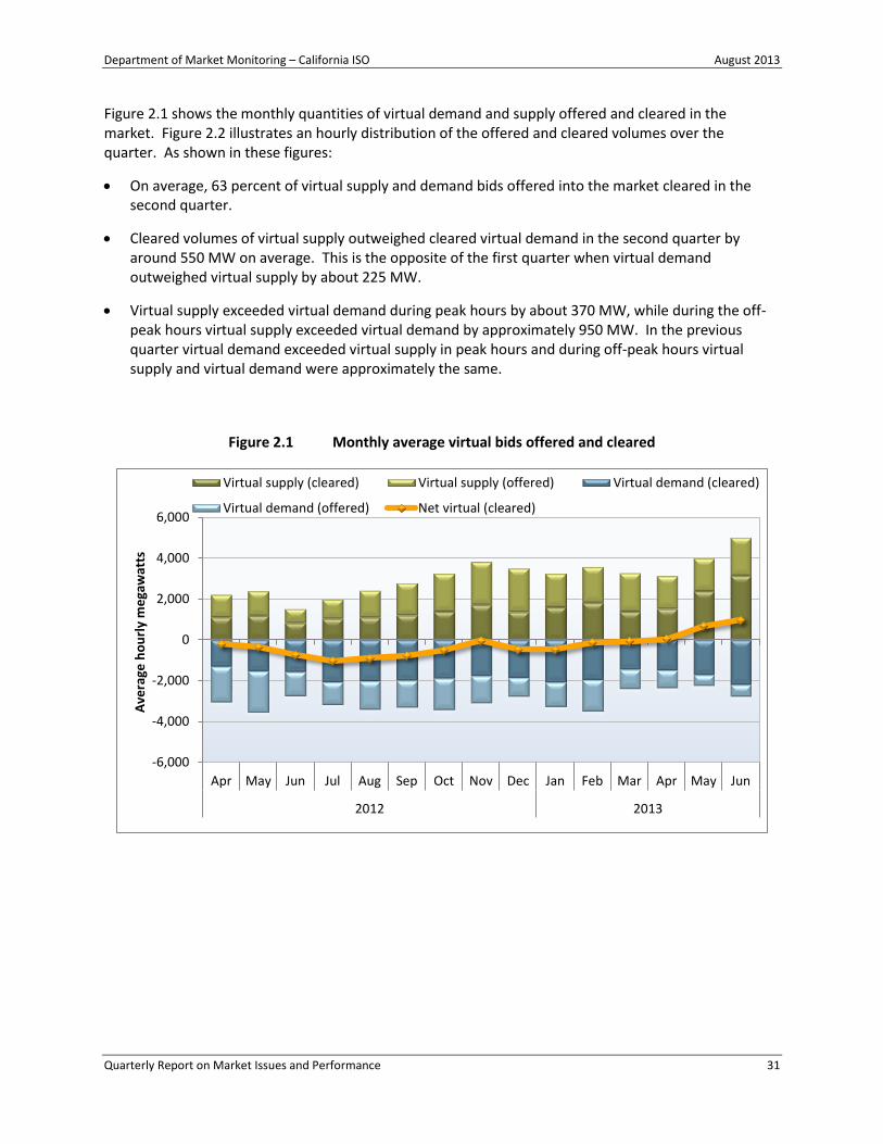
Department of Market Monitoring – California ISO August 2013
Quarterly Report on Market Issues and Performance 31
Figure 2.1 shows the monthly quantities of virtual demand and supply offered and cleared in the market. Figure 2.2 illustrates an hourly distribution of the offered and cleared volumes over the quarter. As shown in these figures:
On average, 63 percent of virtual supply and demand bids offered into the market cleared in the second quarter.
Cleared volumes of virtual supply outweighed cleared virtual demand in the second quarter by around 550 MW on average. This is the opposite of the first quarter when virtual demand outweighed virtual supply by about 225 MW.
Virtual supply exceeded virtual demand during peak hours by about 370 MW, while during the off- peak hours virtual supply exceeded virtual demand by approximately 950 MW. In the previous quarter virtual demand exceeded virtual supply in peak hours and during off-peak hours virtual supply and virtual demand were approximately the same.
Figure 2.1 Monthly average virtual bids offered and cleared
-6,000
-4,000
-2,000
0
2,000
4,000
6,000
Apr May Jun Jul Aug Sep Oct Nov Dec Jan Feb Mar Apr May Jun
2012 2013
Ave
rage
ho
url
y m
ega
wat
ts
Virtual supply (cleared) Virtual supply (offered) Virtual demand (cleared)
Virtual demand (offered) Net virtual (cleared)

Department of Market Monitoring – California ISO August 2013
Quarterly Report on Market Issues and Performance 32
Figure 2.2 Hourly offered and cleared virtual activity (April – June)
Consistency of price differences and volumes
Convergence bidding is designed to bring together day-ahead and real-time prices when the net market virtual position is directionally consistent (and profitable) with the price difference between the two markets. Net convergence bidding volumes were not consistent with price differences in the first quarter of 2013. However, in the second quarter, net convergence bidding volumes were increasingly more consistent with price differences between the day-ahead and real-time markets, with all 24 hours in June consistent with price differences.
Figure 2.3 compares cleared convergence bidding volumes with the volume weighted average price differences at which these virtual bids were settled. The difference between day-ahead and real-time prices shown in this figure represents the average price difference weighted by the amount of virtual bids clearing at different internal locations.
When the red line is positive, it indicates that the weighted average price charged for internal virtual demand in the day-ahead market was higher than the weighted average real-time price paid for this virtual demand. When positive, it indicates that a virtual demand strategy was not profitable and, thus, was directionally inconsistent with weighted average price differences.
Compared to the previous quarter, the overall virtual demand volumes continued to be inconsistent with weighted average price difference for the hours in which virtual demand cleared the market in each month.
During months when the yellow line is positive, this indicates that the weighted average price paid for internal virtual supply in the day-ahead market was higher than the weighted average real-time price
-7,000
-5,000
-3,000
-1,000
1,000
3,000
5,000
7,000
1 2 3 4 5 6 7 8 9 10 11 12 13 14 15 16 17 18 19 20 21 22 23 24
MW
Virtual demand (offered) Virtual demand (cleared)
Virtual supply (offered) Virtual supply (cleared)
Net virtual (cleared)
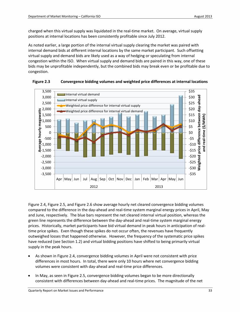
Department of Market Monitoring – California ISO August 2013
Quarterly Report on Market Issues and Performance 33
charged when this virtual supply was liquidated in the real-time market. On average, virtual supply positions at internal locations has been consistently profitable since July 2012.
As noted earlier, a large portion of the internal virtual supply clearing the market was paired with internal demand bids at different internal locations by the same market participant. Such offsetting virtual supply and demand bids are likely used as a way of hedging or speculating from internal congestion within the ISO. When virtual supply and demand bids are paired in this way, one of these bids may be unprofitable independently, but the combined bids may break even or be profitable due to congestion.
Figure 2.3 Convergence bidding volumes and weighted price differences at internal locations
Figure 2.4, Figure 2.5, and Figure 2.6 show average hourly net cleared convergence bidding volumes compared to the difference in the day-ahead and real-time system marginal energy prices in April, May and June, respectively. The blue bars represent the net cleared internal virtual position, whereas the green line represents the difference between the day-ahead and real-time system marginal energy prices. Historically, market participants have bid virtual demand in peak hours in anticipation of real-time price spikes. Even though these spikes do not occur often, the revenues have frequently outweighed losses that happened otherwise. However, the frequency of the systematic price spikes have reduced (see Section 1.2) and virtual bidding positions have shifted to being primarily virtual supply in the peak hours.
As shown in Figure 2.4, convergence bidding volumes in April were not consistent with price differences in most hours. In total, there were only 10 hours where net convergence bidding volumes were consistent with day-ahead and real-time price differences.
In May, as seen in Figure 2.5, convergence bidding volumes began to be more directionally consistent with differences between day-ahead and real-time prices. The magnitude of the net
-$35
-$30
-$25
-$20
-$15
-$10
-$5
$0
$5
$10
$15
$20
$25
$30
$35
-3,500
-3,000
-2,500
-2,000
-1,500
-1,000
-500
0
500
1,000
1,500
2,000
2,500
3,000
3,500
Apr May Jun Jul Aug Sep Oct Nov Dec Jan Feb Mar Apr May Jun
2012 2013
We
igh
ted
pri
ce d
iffe
ren
ce b
etw
ee
n d
ay-a
he
ad
and
re
al-t
ime
($
/MW
h)
Ave
rage
ho
url
y m
ega
wat
ts
Internal virtual demand
Internal virtual supply
Weighted price difference for internal virtual supply
Weighted price difference for internal virtual demand

Department of Market Monitoring – California ISO August 2013
Quarterly Report on Market Issues and Performance 34
virtual supply increased significantly as compared to the previous month. Compared to April, almost twice as many hours (18) were directionally consistent with day-ahead and real-time differences.
Figure 2.6 illustrates improved consistency for net virtual positions in June. In all 24 hours, net convergence bidding volumes were consistent with day-ahead and real-time price differences.
Figure 2.4 Hourly convergence bidding volumes and prices – April
-2,500
-2,000
-1,500
-1,000
-500
0
500
1,000
1,500
2,000
2,500
-$50
-$40
-$30
-$20
-$10
$0
$10
$20
$30
$40
$50
1 2 3 4 5 6 7 8 9 10 11 12 13 14 15 16 17 18 19 20 21 22 23 24
Ne
t vi
rtu
als
wit
hin
ISO
<-
-- D
em
and
Su
pp
ly -
-->
Day
-ah
ead
min
us
real
-tim
e p
rice
Net virtuals (internal supply - internal demand)
Day-ahead minus real-time system marginal price
Net positions are consistent with price differences in 10 hours

Department of Market Monitoring – California ISO August 2013
Quarterly Report on Market Issues and Performance 35
Figure 2.5 Hourly convergence bidding volumes and prices – May
Figure 2.6 Hourly convergence bidding volumes and prices – June
-2,500
-2,000
-1,500
-1,000
-500
0
500
1,000
1,500
2,000
2,500
-$50
-$40
-$30
-$20
-$10
$0
$10
$20
$30
$40
$50
1 2 3 4 5 6 7 8 9 10 11 12 13 14 15 16 17 18 19 20 21 22 23 24
Ne
t vi
rtu
als
wit
hin
ISO
<-
-- D
em
and
Su
pp
ly -
-->
Day
-ah
ead
min
us
real
-tim
e p
rice
Net virtuals (internal supply - internal demand)
Day-ahead minus real-time system marginal price
Net positions are consistent with price differences in 18 hours
-2,500
-2,000
-1,500
-1,000
-500
0
500
1,000
1,500
2,000
2,500
-$50
-$40
-$30
-$20
-$10
$0
$10
$20
$30
$40
$50
1 2 3 4 5 6 7 8 9 10 11 12 13 14 15 16 17 18 19 20 21 22 23 24
Ne
t vi
rtu
als
wit
hin
ISO
<-
-- D
em
and
Su
pp
ly -
-->
Day
-ah
ead
min
us
real
-tim
e p
rice
Net virtuals (internal supply - internal demand)
Day-ahead minus real-time system marginal price
Net positions are consistent with price differences in all 24 hours

Department of Market Monitoring – California ISO August 2013
Quarterly Report on Market Issues and Performance 36
Offsetting virtual supply and demand bids at internal points
Market participants can also hedge congestion costs or earn revenues associated with differences in congestion between different points within the ISO system by placing virtual demand and supply bids at different internal locations during the same hour. These virtual demand and supply bids offset each other in terms of system energy. However, the combination of these offsetting bids can be profitable if there are differences in congestion in the day-ahead and real-time market between these two locations.
The majority of cleared virtual bids in the second quarter were related to these offsetting bids. However, the amount of non-offsetting internal supply increased dramatically since the first quarter. Figure 2.7 shows the average hourly volume of offsetting virtual supply and demand positions at internal locations. The dark blue and dark green bars represent the average hourly overlap between internal demand and internal supply by the same participants. The light green bars represent the remaining portion of internal virtual supply that was not offset by internal virtual demand by the same participants. The light blue bars represent the remaining portion of internal virtual demand that was not offset by internal virtual supply by the same participants.
As shown in Figure 2.7, offsetting virtual positions at internal locations accounted for an average of about 1,420 MW of virtual demand offset by 1,420 MW of virtual supply in each hour of the second quarter. These offsetting bids represent over 68 percent of all cleared internal virtual bids in the second quarter, down from 73 percent of bids in the previous quarter. This suggests that virtual bidding continues to be used to hedge or profit from internal congestion.
Figure 2.7 Average hourly offsetting virtual supply and demand positions by same participants
-3,500
-2,500
-1,500
-500
500
1,500
2,500
3,500
Apr May Jun Jul Aug Sep Oct Nov Dec Jan Feb Mar Apr May Jun
2012 2013
Ave
rage
ho
url
y m
ega
wat
ts
Internal supply offsetting internal demand
Internal demand offsetting internal supply
Non-offsetting internal demand
Non-offsetting internal supply
Vir
tual
su
pp
ly
Vir
tual
de
man
d
Department of Market Monitoring – California ISO August 2013
Quarterly Report on Market Issues and Performance 37
2.2 Convergence bidding revenues
This section highlights sources of net revenues (or payments) received (or paid) by convergence bidders. Unlike the previous quarter, participants engaged in convergence bidding received more money from the ISO markets than what they paid into the ISO markets in the second quarter. This resulted in positive net revenues of about $14 million, with most of the positive revenues associated with virtual supply bids.
Figure 2.8 shows total monthly net revenues for cleared virtual supply and demand. This figure shows the following:
Virtual supply revenues were consistently profitable in every month of the first and second quarters. These revenues were attributed to the higher frequency of negative real-time prices accompanied by congestion and higher convergence bidding volumes.
Virtual demand was unprofitable in every month of the quarter. In total, virtual demand accounted for approximately $18.5 million in net payments to the ISO markets.
Total net revenues paid to virtual bidders increased from the previous quarter. This change was driven by gains on virtual supply positions. Revenues on virtual supply positions increased substantially as virtual bidding volumes increased.
In the second quarter, net revenues paid to convergence bidding entities totaled around $14 million. Virtual demand accounted for around a loss of $18.5 million, while virtual supply generated net revenues of about $32.3 million. This trend reflects that virtual supply positions were paid day-ahead prices that were higher than the real-time prices they received in the second quarter.
Figure 2.8 Total monthly net revenues paid from convergence bidding
-$10
-$5
$0
$5
$10
$15
$20
Apr May Jun Jul Aug Sep Oct Nov Dec Jan Feb Mar Apr May Jun
2012 2013
Tota
l ne
t re
ven
ue
s p
aid
($
mill
ion
s)
Virtual supply net revenue
Virtual demand net revenue
Total net revenues paid

Department of Market Monitoring – California ISO August 2013
Quarterly Report on Market Issues and Performance 38
Net revenues at internal scheduling points
In the second quarter, the cleared share of virtual demand accounted for about 73 percent of bid-in virtual demand at internal locations, up from 53 percent in the previous quarter. Virtual demand bids at internal nodes are profitable when real-time prices spike in the 5-minute real-time market. Almost all net revenues paid for these internal virtual demand positions have resulted from a relatively small portion of intervals when the system power balance constraint becomes binding because of insufficient upward ramping capacity or with congestion. Virtual supply bids are profitable when real-time prices drop below day-ahead prices. Historically, this has happened during off-peak hours when over-generation can drive the real-time prices down. However, in the second quarter, virtual supply positions were increasingly profitable during peak hours.
Figure 2.9 compares total net revenues paid out for internal virtual bids during hours when the power balance constraint was relaxed because of short-term shortages of upward ramping capacity with the overall net revenues of internal virtual bids during all other hours. As shown in Figure 2.9:
Although upward ramping capacity was insufficient in under 0.5 percent of the hours in the quarter, these hours accounted for all net revenues paid for internal virtual demand. Revenues paid for virtual demand during these brief but extreme price spikes can be high enough to outweigh losses when the day-ahead price exceeds the real-time market price. However as with the first quarter, second quarter revenues paid out during these periods were not sufficient to offset virtual demand losses in other periods.
Total net revenues were around $14 million. Virtual demand net revenues were around $6 million during intervals of insufficient upward ramp. Virtual revenues in all other intervals were around $8 million, driven by positive revenues of about $32 million in virtual supply and negative revenues of $24 million in virtual demand in the second quarter.
Figure 2.9 Net revenues paid for convergence bids at internal scheduling points during hours with energy power balance constraint violations due to shortages of upward ramping
-2%
-1%
0%
1%
2%
-$24
-$18
-$12
-$6
$0
$6
$12
$18
$24
Jan Feb Mar Apr May Jun Jul Aug Sep Oct Nov Dec Jan Feb Mar Apr May Jun
2012 2013
Pe
rce
nt
of
ho
urs
wit
h in
suff
icie
nt
up
war
d
ram
p
Tota
l ne
t re
ven
ue
s p
aid
($
mill
ion
s)
Virtual demand revenues in hours with insufficient upward ramp
Revenues in all other hours and virtual positions
Percent of hours with insufficient upward ramp

Department of Market Monitoring – California ISO August 2013
Quarterly Report on Market Issues and Performance 39
Real-time price spikes are typically associated with brief shortages of ramping capacity. Virtual demand at internal scheduling points can potentially result in additional capacity being committed and available in the real-time market. In practice, however, the impact of internal virtual demand on real-time price spikes appears to have been limited by a number of factors:
As discussed in prior sections of this chapter, the impact of virtual internal demand in the day-ahead market was offset significantly by virtual supply.
Any additional capacity potentially made available by convergence bidding may not be enough to address the short-term ramping limitations in the real-time market.
Also, in the event of over-generation, real-time prices can be negative, but rarely fall below the bid floor of -$30/MWh. This diminishes the risk of market participants losing substantial money by bidding virtual demand as well as reduces the potential benefits to virtual supply bids at internal nodes.
Net revenues and volumes by participant type
DMM’s analysis finds that most convergence bidding activity is conducted by entities engaging in pure financial trading that do not serve load or transact physical supply. These entities accounted for $5.8 million (42 percent) of the total convergence bidding settlements in the second quarter and a vast majority of both gains and losses.
Table 2.1 compares the distribution of convergence bidding volumes and revenues among different groups of convergence bidding participants. The trading volumes show cleared virtual positions along with the corresponding revenues in millions of dollars.
DMM has defined financial entities as speculators who own no physical power and participate in only the convergence bidding and congestion revenue rights markets. Physical generation and load are represented by participants that primarily participate in the ISO as physical generators and load-serving entities, respectively. Marketers include participants on the inter-ties and participants whose portfolios are not primarily focused on physical or financial participation in the ISO market.
As shown in Table 2.1, financial participants represent the largest segment of the virtual market, accounting for about 73 percent of volumes and about 42 percent of settlement dollars. Marketers represent about 14 percent of the trading volumes and 22 percent of the settlement dollars. Generation owners and load-serving entities represent a small segment of the virtual market in terms of volumes (about 13 percent); however, they have a significant percent of settlements (approximately 35 percent). Physical participant positions in aggregate were profitable due to revenues from virtual supply positions and have increased in both percentage of net revenues and volume compared to the first quarter.

Department of Market Monitoring – California ISO August 2013
Quarterly Report on Market Issues and Performance 40
Table 2.1 Convergence bidding volumes and revenues by participant type (April – June)
Trading entities Average hourly megawatts Revenues ($ millions)
Virtual demand
Virtual supply
Total Virtual
demand Virtual supply
Total
Financial 375 377 752 -$15.4 $21.2 $5.8
Marketer 53 96 149 -$2.7 $5.8 $3.1
Physical generation 20 65 84 -$0.4 $2.8 $2.4
Physical load 0 50 50 $0.0 $2.5 $2.5
Total 448 588 1,036 -$18.5 $32.3 $13.8

Department of Market Monitoring – California ISO August 2013
Quarterly Report on Market Issues and Performance 41
3 Special Issues
3.1 Greenhouse gas cap-and-trade program
Generating resources became subject to California’s greenhouse gas cap-and-trade program compliance requirements starting on January 1, 2013. This section highlights the impact of these requirements in the first and second quarters. These highlights include the following:
The cost of greenhouse gas emissions permits has been stable, averaging $14.55/mtCO2e for the first quarter and $14.59/MtCO2e for the second quarter.22
Imports do not appear to have decreased in response to implementation of the cap-and-trade program. In fact, import schedules and bid-in volumes increased in the first half of 2013 compared to the first half of 2012.
Based on statistical analysis of changes in day-ahead market energy prices following the cap-and-trade implementation, DMM estimates that average wholesale prices are about $6/MWh or about 15 percent higher in the first half of 2013 due to cap-and-trade compliance costs. This is also consistent with the emissions costs for gas units typically setting prices in the ISO market.
Background
California Assembly Bill 32 (AB 32), the Global Warming Solutions Act of 2006, directs the California Air Resources Board (CARB) to develop regulation to reduce greenhouse gas emissions to 1990 levels by 2020. The cap-and-trade program is one of a suite of regulatory measures adopted by CARB to achieve this goal.
The cap-and-trade program covers major sources of greenhouse gas emissions including power plants.23 The program includes an enforceable emissions cap that will decline over time. California will directly distribute and auction allowances, which are tradable permits equal to the emissions allowed under the cap.
The impact of higher wholesale prices on retail electric rates will depend on policies adopted by the CPUC and other state entities. As part of the cap-and-trade program, the CARB allocated allowances to the state’s electric distribution utilities to help compensate electricity customers for the costs that will be incurred under cap and trade. The investor-owned electric utilities are required to sell all of their allowances at CARB’s quarterly auctions, and the proceeds from the auction are to be used for the
22
mtCO2e stands for metric tons of carbon dioxide equivalent, a standard emissions measurement. 23
The cap-and-trade program covers major sources of greenhouse gas emissions in California such as refineries, power plants, industrial facilities, and transportation fuels. For the electricity sector, the covered entity is the first deliverer of electricity. The first deliverer is defined in the regulation as the operator of an in-state electricity generator, or an electricity importer. The compliance obligation for first deliverers is based on the emissions that are a result of the electricity they place on the grid. The threshold for inclusion in the program for electricity generated from an in-state facility, and for imported electricity from a specified source, is 25,000 metric tons of annual greenhouse gas emissions. For imported electricity from unspecified sources, there is no threshold and all emissions are covered.

Department of Market Monitoring – California ISO August 2013
Quarterly Report on Market Issues and Performance 42
benefit of retail ratepayers, consistent with the goals of AB 32. Under a 2012 CPUC decision, revenue from carbon emission allowances sold at auction will be used to offset impacts on retail costs.24
One allowance represents one metric ton of CO2e. Sources under the cap are required to surrender allowances and offsets equal to their emissions at the end of each compliance period, with a partial annual surrender in the interim years. Electric generation resources emitting more than 25,000 metric tons of greenhouse gas annually, either within California or as imports into California, are covered under the first phase of the cap-and-trade program, which started on January 1, 2012, with enforceable compliance obligations beginning with emissions during 2013.
AB 32 requires CARB to minimize leakage, which is a reduction in greenhouse gas emissions within California that is offset by an increase in greenhouse gas emissions outside of California. The cap-and-trade program limits leakage in part by prohibiting resource shuffling, or substituting imports of lower gas emitting resources for imports actually sourced from higher emitting resources to avoid the cost of allowances. Proposed cap-and-trade regulation changes that incorporate resource shuffling definitions into the regulation and clarify resource shuffling safe harbors were released in draft form in July and are scheduled for CARB’s Board consideration in October of this year.25 The proposed rule changes would also permanently eliminate a temporarily waived requirement that market participants attest each year that they have not engaged in resource shuffling.26
Generators and importers that are covered by the regulations are required to submit allowances covering 30 percent of emissions in each year and the remainder of their emissions in the final year of each three year compliance period. In addition to allowances, covered generators and importers may submit emissions offsets to cover up to 8 percent of their emissions. The total cap on emissions is set to decline 2 percent annually through 2014 and then about 3 percent annually through 2020.
Allowances are available at quarterly auctions held by the Air Resources Board and may also be traded bilaterally. In addition, financial derivatives based on allowance prices are traded on public exchanges such as the InterContinental Exchange (ICE). Allowances are associated with a specific year, which is known as the vintage. Allowances are bankable, meaning that an allowance may be submitted for compliance in years subsequent to the vintage of the allowance.27 Borrowing of allowances is not
24
Pursuant to CPUC decision Docket #R.11-03-012, the investor-owned utilities will distribute this revenue to emissions-intensive and trade-exposed businesses, to small businesses, and to residential ratepayers to mitigate carbon costs. Remaining revenues will be given to residential customers as an equal semi-annual bill credit. See http://docs.cpuc.ca.gov/PublishedDocs/Published/G000/M039/K594/39594673.PDF.
25 The proposed regulation changes are posted here: http://www.arb.ca.gov/cc/capandtrade/meetings/071813/ct_reg_2013_discussion_draft.pdf. A presentation describing the proposed cap-and-trade program regulation changes is available here: http://www.arb.ca.gov/cc/capandtrade/meetings/071813/workshoppresentation.pdf. Also, see CARB Regulatory Guidance document: What is Resource Shuffling, dated November 2012 http://www.arb.ca.gov/cc/capandtrade/guidance/appendix_a.pdf.
26 See proposed regulation cited above and the letter from the CARB Chairman Mary Nichols to Commissioner Moeller of the Federal Energy Regulatory Commission dated August 16, 2012: http://www.arb.ca.gov/newsrel/images/2012/response.pdf.
27 For example, a vintage 2013 allowance may be used for compliance during either the first (2013-2014), second (2015-2017), or third (2018-2020) compliance periods.

Department of Market Monitoring – California ISO August 2013
Quarterly Report on Market Issues and Performance 43
allowed, meaning that permits for future years cannot satisfy compliance requirements in an earlier year.28
The cap-and-trade program affects wholesale electricity market prices in two ways. First, market participants covered by the program will presumably increase bids to account for the incremental cost of greenhouse gas allowances. Second, the ISO amended its tariff, effective January 1, 2013, to include greenhouse gas compliance cost in the calculation of each of the following:
Resource commitment costs (start-up and minimum load costs);
Default energy bids, which are bids used in the automated local market power mitigation process; and
Generated bids (bids generated on behalf of resource adequacy resources and as otherwise specified in the ISO tariff).29
The ISO uses a calculated greenhouse gas allowance index price as a daily measure of the cost of greenhouse gas allowances. The ISO greenhouse gas allowance price is calculated as the average of two market based indices.30 Daily values of the ISO greenhouse gas allowance index are plotted in Figure 3.1.
After rising to over $16/mtCO2e in the first week of 2013, the ISO greenhouse gas allowance index prices dropped and were fairly constant, varying between $13.50/mtCO2e and $15/mtCO2e. The average value of the index was $14.59/mtCO2e in the second quarter, slightly above the average value for the first quarter: $14.55/mtCO2e.
28
The proposed cap-and-trade regulation changes add an exception to allow limited borrowing for true-up allowances, allowances allocated for production changes or allowance allocation not properly accounted for in prior allocations. http://www.arb.ca.gov/cc/capandtrade/meetings/071813/ct_reg_2013_discussion_draft.pdf.
29 Details on each of the calculations may be found in the ISO Business Practice Manual for Market Instruments, Appendix K: http://bpmcm.caiso.com/BPM Document Library/Market Instruments/BPM_for_Market_Instruments_v26_clean.doc.
30 The indices are ICE and ARGUS Air Daily. As the ISO noted in a market notice issued on May 8, the ICE index is a settlement price but the ARGUS price was updated from a settlement price to a volume weighted price in mid-April of this year. For more information, see the ISO notice: http://www.caiso.com/Documents/GreenhouseGasAllowancePriceSourcesRevisedMay8_2013.htm.

Department of Market Monitoring – California ISO August 2013
Quarterly Report on Market Issues and Performance 44
Figure 3.1 ISO's greenhouse gas allowance price index
Effects in import levels and participation
Nearly 30 percent of ISO load was served by imports from outside the ISO system in 2012, with most of these imports coming from outside California.31 Prior to the implementation of the cap-and-trade program, stakeholders and regulators were concerned that certain rules related to resource shuffling would result in reduced imports into California as some participants would elect to no longer import.32 Ultimately, while the mix of participants that import power into California has changed slightly in 2013, the levels of imports have increased in the first half of 2013, compared to the first half of 2012.33
Figure 3.2 shows the amount of megawatts bid in at inter-ties and cleared in the day-ahead market in the first half of 2012 and 2013.34 Percentages in the boxes in Figure 3.2 highlight the percentage change in total volume of import bids offered each month in 2013 compared to the same month in 2012. In the first half, the total amount of import megawatts offered to the market increased for each month in 2013 compared to the first half of 2012. Overall, import megawatts offered increased by 13 percent in the first half of 2013 compared to the first half of 2012.
31 See the DMM 2012 Annual Report on Market Issues and Performance, Section 1.2 on supply conditions:
http://www.caiso.com/Documents/2012AnnualReport-MarketIssue-Performance.pdf. 32
See the August 6 letter from FERC Commissioner Moeller to Governor Brown: http://www.ferc.gov/about/com-mem/moeller/moeller-08-06-12.pdf.
33 There were a small number of participants, specifically, public entities, and their associated imports into California, which explicitly stopped importing as a result of the program. However, new market entrants have begun to import into California and include a mix of public entities and private companies. In total, the new entrant imports exceeded the quantity of megawatts that were associated with the participants that are no longer importing into California.
34 This analysis excludes imports from dynamic system units and wheels.
$12.00
$12.50
$13.00
$13.50
$14.00
$14.50
$15.00
$15.50
$16.00
$16.50
$17.00
Jan Feb Mar Apr May Jun
Gre
en
ho
use
gas
allo
wan
ce p
rice
ind
ex
($/m
tCO
2e
)

Department of Market Monitoring – California ISO August 2013
Quarterly Report on Market Issues and Performance 45
As shown by the darker bars in Figure 3.2, the volume of import bids that cleared the market also increased each of the first four months of 2013 compared to 2012. In May and June the volume of import bids clearing the market dropped slightly compared to 2012 though the overall bid-in import volumes were higher. Overall, import megawatts cleared in the market during the first six months of 2013 increased by 7 percent compared to 2012.
Figure 3.2 Inter-tie imports offered and cleared in the day-ahead market
Bid prices for imports have increased notably in the first six months of 2013 compared to 2012. However, DMM attributes most of this increase to the increase in gas prices, which have risen by about 50 percent over this period. Given the significant change in gas prices over this period, DMM has not sought to quantify the portion of higher import bid prices that may be attributable to greenhouse gas allowance costs.
Changes in market prices
Greenhouse gas compliance costs are expected to increase wholesale electricity costs as both market participant bids and the ISO’s own calculation of default energy bids, resource commitment costs and generated bids increase to reflect the additional incremental variable cost of greenhouse gas compliance.
DMM has adopted a statistical approach to estimate the impact of greenhouse gas costs on day-ahead market prices during the first and second quarters of greenhouse gas compliance. This approach relies on the comparison of market data before cap-and-trade implementation with data from the first half of
0
2,000
4,000
6,000
8,000
10,000
12,000
14,000
2012 2013 2012 2013 2012 2013 2012 2013 2012 2013 2012 2013
Jan Feb Mar Apr May June
Ave
rage
ho
url
y m
ega
wat
ts
Imports cleared Imports offered (not cleared) Imports cleared Imports offered (not cleared)
+31 % +18 % +12 %
+9 % +8 % +5 %

Department of Market Monitoring – California ISO August 2013
Quarterly Report on Market Issues and Performance 46
2013.35 DMM used a similar model in the first quarter, but improved upon it to control for exogenous differences in generation availability (wind, for example) and other factors.36 The improved model allows us to broaden the time period of analysis to include the second quarter of 2013.
The energy price DMM chose to analyze was the day-ahead system marginal energy cost.37 DMM chose to analyze changes in this value to limit the effects of transmission congestion when trying to isolate the effect of the greenhouse gas costs. While the system marginal energy cost does not eliminate transmission congestion effects, it can act as a reasonable benchmark for system prices.38
DMM estimates the impact of greenhouse gas compliance on wholesale energy prices by estimating average daily system energy prices as a linear function of a measure of greenhouse gas compliance cost, gas price indices, indicator variables for holidays, Saturday, and Sunday, and a non-linear function of expected load, scheduled generation availability for fuel types that we assume to be exogenous (hydro, wind, solar, geo-thermal, and nuclear), and imports (as modeled by exogenous gas price indices).39
35
As demonstrated in Figure 3.1, the ISO’s estimated greenhouse gas compliance cost does not exhibit sufficient variation to determine the impact based on minor fluctuations in this value alone.
36 A summary of our earlier analysis is available in the Quarterly Report on Market Issues and Performance for Q1 2013: http://www.caiso.com/Documents/2013FirstQuarterReport-MarketIssues_Performance-May2013.pdf.
37 This is the energy component of each of the locational marginal prices within the ISO system and excludes both congestion and transmission loss related costs.
38 For further discussion on the system marginal energy price, please see Appendix C of the ISO tariff: http://www.caiso.com/Documents/CombinedConformedTariff_Mar20_2013.pdf.
39 If import supply is elastic, imports may be endogenous. That is, scheduled imports may themselves be a function of electricity prices. Including an endogenous variable in the regression could bias our results, so DMM has used an instrumental variable approach to estimate the impact of greenhouse gas emission costs in a consistent manner. A useful set of instruments has two properties. First, the set should be a powerful predictor of the endogenous factor: imports. Second, the instruments should not be endogenous themselves. For this analysis, DMM uses daily gas price indices for multiple hubs outside of the ISO to instrument import levels. DMM’s model is estimated using two stage least squares estimated with the ivreg() function of the AER package (Christian Kleiber and Achim Zeileis (2008). Applied Econometrics with R. New York: Springer-Verlag. ISBN 978-0-387-77316-2. http://CRAN.R-project.org/package=AER.) available in R (R Core Team (2013). R: A language and environment for statistical computing. R Foundation for Statistical Computing, Vienna, Austria. http://www.R-project.org/.)

Department of Market Monitoring – California ISO August 2013
Quarterly Report on Market Issues and Performance 47
Using this model, DMM estimates that in the first six months of 2013 the impact of greenhouse gas compliance was about $6/MWh or $0.40 per dollar of the allowance price.40 Although rough, our model predicts the average ISO day-ahead system energy prices fairly well, explaining approximately 92 percent of the variation in this measure in both models.41 This analysis may be refined as further data becomes available.
The statistical approach outlined above produces estimates that are highly consistent with expectations of the impact of greenhouse gas compliance costs on wholesale electricity costs during a period when market prices are being set close to the marginal operating cost of relatively efficient units. For example, given an average emission cost of $14.59/mtCO2e, an additional cost of $6.21/MWh represents the emission cost of a gas-fired unit with a heat rate of 8,000 Btu/kWh.42
Figure 3.3 illustrates average monthly implied heat rates with and without an adjustment for greenhouse gas compliance costs. The implied heat rate is a standard measure of the maximum heat rate that would be profitable to operate given electricity prices and fuel costs, ignoring all non-fuel costs. The implied heat rate is calculated by dividing the electricity price, in this case the hourly day-ahead system marginal energy price, by fuel price. Because natural gas is often on the margin in the ISO market, we use a weighted average of daily natural gas prices.43
DMM calculates the implied heat rate adjusted for greenhouse gas compliance costs by subtracting our estimate of the greenhouse gas compliance cost price impact derived above from the energy price and then dividing the result by the gas price index. This analysis shows that changes in gas prices and greenhouse gas compliance costs account for almost all of the electricity price increase between the first six months of 2012 and 2013.
40
Two alternative greenhouse gas measures are used. The first is an indicator variable equal to 1 in the greenhouse gas compliance period and 0 before that period. In this case, the coefficient estimate (β1 in the equation above) may be interpreted as the estimated average impact of greenhouse gas compliance on electricity prices ($/MWh). The second greenhouse gas measure is the ISO’s index of the greenhouse gas allowance value, set equal to zero before the compliance period. In this case, the coefficient estimate may be interpreted as the estimated impact of greenhouse gas compliance per allowance cost ($/MWh divided by $/mtCO2e). DMM’s regression results are based on values from January 2012 through June 2013 to limit bias introduced by factors not yet included in the model. Load is the ISO’s hourly day-ahead forecast of ISO load. We assume that the load forecast, which is based on weather indices and historical time series data, is not price responsive in the short-term, which allows us to estimate this model using ordinary least squares, rather than as a system of demand and supply equations. We also assume that the greenhouse gas allowance index price is exogenous rather than endogenously determined by electricity prices. Resource specific day-ahead schedules are summed by fuel type to calculate the wind, geothermal, nuclear, solar, hydro, and imports. As discussed in footnote 39 imports are estimated as a linear function of the remaining exogenous independent variables and instrumented by multiple gas price indices outside of California.
41 In the first case, R
2 = 0.9234 and the adjusted R
2 = 0.9200. In the second case, R
2 = 0.9236 and the adjusted R
2 = 0.9203.
42 $14.59/mtCO2e x 0.053165 mtCO2/MMBtu x 8,000 Btu/kWh = $6.21/MWh
43 For this calculation, DMM is using a weighted average of three regional gas price indices (weights are given in parentheses): PGE2 (0.4), SCE1 (0.5), and SCE2 (0.1). These gas price indices are used by the ISO in calculating default energy bids and other market calculations.
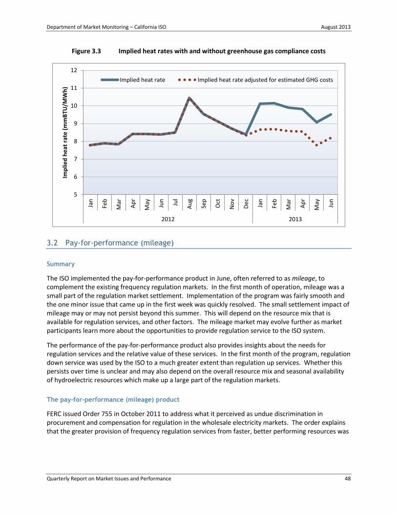
Department of Market Monitoring – California ISO August 2013
Quarterly Report on Market Issues and Performance 48
Figure 3.3 Implied heat rates with and without greenhouse gas compliance costs
3.2 Pay-for-performance (mileage)
Summary
The ISO implemented the pay-for-performance product in June, often referred to as mileage, to complement the existing frequency regulation markets. In the first month of operation, mileage was a small part of the regulation market settlement. Implementation of the program was fairly smooth and the one minor issue that came up in the first week was quickly resolved. The small settlement impact of mileage may or may not persist beyond this summer. This will depend on the resource mix that is available for regulation services, and other factors. The mileage market may evolve further as market participants learn more about the opportunities to provide regulation service to the ISO system.
The performance of the pay-for-performance product also provides insights about the needs for regulation services and the relative value of these services. In the first month of the program, regulation down service was used by the ISO to a much greater extent than regulation up services. Whether this persists over time is unclear and may also depend on the overall resource mix and seasonal availability of hydroelectric resources which make up a large part of the regulation markets.
The pay-for-performance (mileage) product
FERC issued Order 755 in October 2011 to address what it perceived as undue discrimination in procurement and compensation for regulation in the wholesale electricity markets. The order explains that the greater provision of frequency regulation services from faster, better performing resources was
5
6
7
8
9
10
11
12
Jan
Feb
Mar
Ap
r
May Jun
Jul
Au
g
Sep
Oct
No
v
De
c
Jan
Feb
Mar
Ap
r
May Jun
2012 2013
Imp
lied
he
at r
ate
(m
mB
TU/M
Wh
)
Implied heat rate Implied heat rate adjusted for estimated GHG costs

Department of Market Monitoring – California ISO August 2013
Quarterly Report on Market Issues and Performance 49
not recognized in the RTO and ISO markets. To remedy this situation, the FERC ordered that each ISO or RTO institutes a market-based system that compensates regulation performance.44
The ISO implemented the pay-for-performance product on June 1, 2013. The product is directional, meaning that mileage up and mileage down are separate services. These services are procured in both the day-ahead and real-time markets along with other ancillary services.
The term mileage refers to the amount of movement that a resource performs while providing regulation service to the ISO system. Energy deployments of regulation service are measured across four-second intervals. Previously, units were compensated for regulation capacity and then also paid the market price for the real-time net energy they provided while performing regulation services on ten-minute intervals. As Automatic Generation Control (AGC) signals are sent every four seconds, the compensation of regulation capacity and energy over the settlement period does not reflect the quality of the regulation service that the generator provides in responding to the control signal.
Resources that sell mileage in the ISO market under the new program receive a payment for available regulation capacity in a similar manner as before, but also receive a payment for the amount of up and down movement they actually deliver. Thus, mileage is a measure of the service that is derived from resources providing regulation capacity.
While units submit separate offer prices for regulation capacity and mileage, the mileage product is procured from the set of resources that have also sold regulation capacity. The joint procurement results in the market preferring to procure regulation from units that can move quickly and follow the regulation signal accurately. Resources that are eligible to provide regulation can bid into the mileage market at a price ranging from $0 to $50 per megawatt of mileage, where each megawatt of mileage represents one megawatt of regulation service provided in a given direction.
Any resource should be able to provide a quantity of mileage at least equal to its regulation capacity. In other words, if a resource provides 10 MW of regulation, it must be able to change its output by at least 10 MW.45 Since mileage is measured over an hour, and can consist of both up and down movement, it is also possible that a regulation resource may provide significantly more total movement in an hour than is indicated by its regulation capacity.
The amount of mileage a unit may sell is determined by the resource’s history of accurately following AGC signals and its ramp rate. Resources do not respond perfectly to the AGC signal, so the amount of mileage that is instructed is not the same as what is delivered. Settlements are based on the adjusted mileage, with corrections for measured accuracy.
The total system requirement for mileage for each trading hour is determined using a rolling average of the amount of instructed mileage in that hour over the last seven days scaled by the amount of regulation procured in each hour. A historical measure is used because it is not possible to know in advance how much movement will be required of the regulating resources. This means that the amount of mileage procured in the market is an estimate of the system need for that hour and will differ from the amount of mileage that is actually provided. There are no constraints or bounds that relate the
44
For further detail, see 18 C.F.R. § 35.28(g)(3) http://www.ferc.gov/whats-new/comm-meet/2011/102011/E-28.pdf. 45
As part of the pay-for-performance design, the definition of regulation capacity available from a given resource was standardized to be equal to the amount that the resource can ramp in ten minutes.

Department of Market Monitoring – California ISO August 2013
Quarterly Report on Market Issues and Performance 50
market results to actual mileage provision other than the amount of regulation reserve capacity procured from each resource.
Mileage market performance
Mileage prices were low in both directions in June averaging $0.16 for mileage down and $0.03 for mileage up in the day-ahead market. Real-time prices were similarly low, averaging $0.09 for mileage down and $0.03 for mileage up. Estimated mileage payments were $11,300 for mileage up and $52,400 for mileage down.
Peak prices for mileage up generally corresponded to peak levels of quantity demanded. Peak prices for mileage down appeared to be driven by other factors, with higher prices potentially driven by lower gross available supply that is characteristic during certain times of the day. Mileage prices and quantities are divided into directional categories which correspond with regulation. The system needs for regulation services in either direction vary throughout the day.
Figure 3.4 shows the average hourly levels of adjusted upward mileage in June as well as the average mileage up price and regulation up price in each hour from the day-ahead market.46 System needs for regulation up service in the form of mileage peaked in hour ending 7 at about 677 MW of mileage up. The price peak for mileage occurred in the same hour at about $0.13 per megawatt of service. At that time the average price of regulation up capacity was about $0.67 per megawatt, which is close to the daily low. Peak average prices for regulation up capacity come at hour ending 17 at a price of more than $16/MW. At that time, the average price for mileage up was less than $0.01.
The divergence in price over the day between regulation up capacity and mileage up reflects that regulation up capacity is co-optimized with energy and mileage up is not. The regulation price can, therefore, be affected by opportunity costs of energy production, which do not factor directly into the mileage up price.
The peak in adjusted upward mileage at hour ending 7 is about double the average hourly adjusted mileage. While quantities vary from day to day, this value does not appear to be driven by a single incident or outlier. Instead, it appears that regulation service in the upward direction is commonly needed in that time period in larger quantities than other hours. This may be a trend that varies seasonally.
Figure 3.5 shows the monthly average of adjusted mileage down throughout the day, as well as the averages of the mileage down prices and the price of regulation down reserves from the day-ahead market. Downward mileage was most valuable in the early morning, as evidenced by the higher prices, up to $0.70 in hours ending 2, 5, 6, and 7. Even though prices were high in those hours, the quantities of mileage down were small at those times, averaging from 350 MW to just under 900 MW, compared to an average of over 1,200 MW per hour for the whole day.
Adjusted mileage down quantity peaked at hour ending 22 with an average of 1,913 MW of adjusted mileage. For that hour, the average price was about $0.10 per MW of mileage. The value of regulation
46
Adjusted mileage is the instructed mileage corrected for resource under-response. It does not exactly represent service rendered to the system, but is indicative of regulation service demands. The term actual mileage throughout the document also means the same.

Department of Market Monitoring – California ISO August 2013
Quarterly Report on Market Issues and Performance 51
down service in the early morning may be related to scarcity. During this period, many resources were already ramped down to lower output levels and were not able to provide further decremental energy.
Figure 3.4 Mileage up price and adjusted quantity
Figure 3.5 Mileage down price and adjusted quantity
$0
$2
$4
$6
$8
$10
$12
$14
$16
$18
0
100
200
300
400
500
600
700
800
900
1 2 3 4 5 6 7 8 9 10 11 12 13 14 15 16 17 18 19 20 21 22 23 24
Pri
ce (
$/M
W)
Mile
age
up
(M
W)
Trade hour
Adjusted mileage
Mileage up price
Regulation up price
$0
$1
$2
$3
$4
$5
$6
0
400
800
1,200
1,600
2,000
2,400
1 2 3 4 5 6 7 8 9 10 11 12 13 14 15 16 17 18 19 20 21 22 23 24
Pri
ce (
$/M
W)
Mile
age
do
wn
(M
W)
Trade hour
Adjusted mileage
Mileage down price
Regulation down price
Department of Market Monitoring – California ISO August 2013
Quarterly Report on Market Issues and Performance 52
As shown in Figure 3.5, system regulation down needs roughly correspond to load. The exception to this general trend is that the late-night downward ramp also requires high amounts of regulation down service. Meanwhile, the need for regulation service in the downward direction has not been closely correlated to the mileage down price.
Significant amounts of regulation were procured in both directions throughout the day and even at times when mileage prices were at or near zero on average. One of the conditions that allowed for frequent zero prices was a robust supply of zero price mileage bids available to the ISO market. In order to be procured, these mileage bids must be tied to regulation bids that also clear the market. This supply of zero price bids is one of the factors that kept the cost of mileage low in the month of June.
Figure 3.6 shows the quantities of mileage up that were required by the market, procured by the market, and the adjusted quantity that represents system instructions to resources. Upward mileage is often procured at a zero price, which allows the system to procure more than the market requirement without penalty. This can be seen in the graph during all hours, where the average procured mileage was above the requirement.
Adjusted mileage up and required mileage up follow a similar pattern throughout the day. Required mileage is actually a rolling seven day average of instructed mileage, and adjusted mileage is corrected for resource response of instructed mileage. The differences in these two numbers are due to resource response and to slightly different sampling.47 The sampling difference is significant because the sample is drawn from only 30 days of data.
The price of mileage down is less frequently near zero when compared to mileage up. This can be seen in Figure 3.7 where the procured quantity of mileage down was very close to the required quantity, on average, through much of the day. The mileage down price was $0 most frequently during hours ending 14 through 20, and over-procurement of mileage down was most often seen at those times. The pattern of requirement and procurement throughout the day is similar to the pattern of adjusted mileage down.
The system need for mileage down was generally greater than the need for mileage up in June. Downward services are used about three times as much as upward services and could be the result of seasonal effects. In contrast to regulation service needs, required quantities of regulation capacity are often at or near the same level in either direction. When they do separate, the required quantity of regulation up is usually the higher of the two. However, monitoring mileage use may help inform the ISO in setting regulation reserve requirements at different times of the day and year.
47
The requirement starts with seven days of data at day one and places less weight on the last seven days of the month in return.

Department of Market Monitoring – California ISO August 2013
Quarterly Report on Market Issues and Performance 53
Figure 3.6 Mileage up quantity required, procured, and adjusted
Figure 3.7 Mileage down quantity required, procured, and adjusted
0
100
200
300
400
500
600
700
800
900
1,000
1 2 3 4 5 6 7 8 9 10 11 12 13 14 15 16 17 18 19 20 21 22 23 24
Mile
age
up
(M
W)
Trade hour
Market mileage up requirement (MW)
Adjusted mileage up (MW)
Procured mileage up (MW)
0
500
1,000
1,500
2,000
2,500
3,000
1 2 3 4 5 6 7 8 9 10 11 12 13 14 15 16 17 18 19 20 21 22 23 24
Mile
age
do
wn
(M
W)
Trade hour
Market mileage down requirement (MW)
Adjusted mileage down (MW)
Procured mileage down (MW)

Department of Market Monitoring – California ISO August 2013
Quarterly Report on Market Issues and Performance 54
Performance accuracy
An important part of FERC order 755 and of the ISO’s pay-for-performance regulation program is the measurement of resource accuracy. The ISO has a benchmark of 50 percent accuracy that a resource must meet to continue to be a regulation resource. However, in the first month of the mileage program the system-wide accuracy was near or below this standard. On average, the performance accuracy was 53 percent for mileage down and 40 percent for mileage up in June. This number is a simple average of the measured accuracies for each 15-minute interval. Using an average weighted by the amount of instruction, the system accuracy for mileage down in June was 64 percent and 55 percent for mileage up.
Accuracy is measured for each resource by comparing the resource’s output to the AGC signal instructions at each four-second interval. All intervals where the AGC signal instructs the resource to move at least 0.1 MW or 0.1 percent of the resource’s regulation capacity will count towards the accuracy calculation. This means that accuracy is only being counted when the AGC signal is asking the resource to make a real change in output. One result of this exception is that the minor variations that a resource may exhibit when it is holding steady and not being asked for movement will not result in a decreased accuracy rating. Accuracy calculations are made for each 15-minute interval by aggregating data from all of the relevant four second intervals.
Table 3.1 categorizes resources that sold mileage by technology type and shows the average accuracy, weighted by instructed mileage, for each type of resource. Gas powered combined cycle generators were the most accurate as a class but are slightly slower in ramping than hydro resources that are used more by the AGC system. Steam turbines are rarely used and slower in ramping than the other types, and were the least accurate.48 The reason that the market buys more regulation service from hydro rather than the more accurate gas combined cycles is most likely related to energy bids and timing. Hydro resources have run limitations, but are more often available during off-peak hours. Combined cycles may be offline or operating at their minimum at these times and so cannot provide downward regulation services.
Table 3.1 Mileage performance accuracy by technology type
48
Pump storage hydro and gas combustion turbines made up less than 0.02 percent of market procurements of regulation service and so are excluded from this table.
Up Down Up Down Up Down
Gas-powered combined cycle 20 61% 71% 42% 60% 21% 22% 1,750
Hydroelectric 22 56% 63% 40% 52% 71% 76% 2,113
Gas-powered steam turbine 7 26% 49% 18% 40% 7% 2% 1,063
Total system 21 55% 64% 40% 53% 6,087
Technology type
Accuracy using weighted
average
Accuracy using
simple averageAverage ramp
rate (MW/min)
Share of total
instructions
Regulation
capacity
(MW)

Department of Market Monitoring – California ISO August 2013
Quarterly Report on Market Issues and Performance 55
Table 3.1 indicates that the system level average is below the standard of 50 percent accuracy for mileage up and is only marginally above the standard for mileage down.49 The table also shows the marked difference when accuracy is weighted by the amount of instructed mileage for each resource. Weighting allows for a more accurate picture of the relationship between mileage requested and mileage received. Weighting also minimizes the accuracy impacts of intervals with instructions that represent small deviations from a unit’s dispatch point.
There are two issues regarding the accuracy calculation used by the ISO. The first is the difference between the simple averages and the weighted averages in Table 3.1. This difference suggests that the simple averages understate the amount of mileage that the system receives relative to the amount it instructs by placing equal emphasis on periods of small needs and periods of large needs. The second relates to the difference between accuracy and precision, or repeatability. While the mileage instructed by the system differs from actual delivery, it may differ in a knowable, predictable way.
DMM has examined system level mileage performance by comparing mileage instructed and mileage received using statistical regression analysis. The results yield regression coefficients far below one, indicating the ISO system receives less regulation service than it asks for. However, the correlation between mileage instructed and mileage received varied from 85 percent to 97 percent. These results suggest that the system instructs more mileage than is needed but the relationship between instruction and delivery is consistent over time. Variation in service that would be explained by randomness or factors outside of the AGC system is relatively small.
Possible explanations have been posed for the low accuracy figures, including the AGC system not properly accounting for resource characteristics, telemetry issues, and time lag in resource response to AGC signals possibly being different than what the system expects. The ISO plans to investigate this under-response, or over-instruction, in the near future.
One of the primary areas of concern surrounding regulation performance accuracy is that of resource disqualification. Currently, the ISO’s business practice manual states that resources that fail the minimum performance threshold of 50 percent accuracy using a simple average of 15 minute accuracy measurements over a calendar month will receive notification of the need to recertify the resource to provide that regulation service within 90 days or face disqualification from the ability to provide that service. In June, 42 of the 49 resources that sold regulation up to the ISO fell short of this threshold.
Recertifying (or disqualifying) these resources could significantly shift the market for regulation up to a set of resources that may or may not perform better. Such a shift would potentially yield a subset of resources that meet the performance criteria, as well as an increase in the cost of regulation up service. If the correct accuracy criteria are used, this would likely move the regulation market to those resources that provide the quickest and most accurate response and likely improve the ISO’s regulation market performance. If the weighted average is appropriate, however, using the simple average to disqualify resources would lead to unnecessary cost increases and possible market power concerns.
49
These are averages comprised of a range of performance from individual resources, some of which did not meet the minimum performance standard.

Department of Market Monitoring – California ISO August 2013
Quarterly Report on Market Issues and Performance 56
Implementation issues
The pay-for-performance product has had few unexpected implementation issues. One primary issue was related to an unanticipated ability of the system to procure more than the required amount of regulation capacity or of mileage. Some of these instances resulted in zero or negative mileage prices in both directions. The ISO corrected these negative prices.
On the mornings of June 4, 5 and 6, regulation prices in the real-time market were negative for periods of one to four 15-minute real-time intervals. At the same time, the ISO procured up to 100 MW of regulation up or down capacity in excess of the market requirement. These two items are directly related through the mileage requirements and the mechanics of mileage and ancillary services procurement.
The market sets a minimum mileage requirement that must be procured in each interval. It also has a minimum requirement for regulation capacity. Because ancillary services bids are often submitted with a zero price, there were previous issues with over procurement of ancillary services. At times the zero priced capacity would be reserved for ancillary services in the 15-minute real-time pre-dispatch market, making it unavailable to provide energy in the real-time dispatch.
To avoid this, a parameter was set in the system to limit the maximum amount of regulation procured and set a negative price. This negative price then would prevent the system from buying excessive amounts of zero priced ancillary services over the requirement. However, because the mileage and regulation prices are linked, it became possible for the market to buy mileage at a positive price above the bid price along with regulation at a negative price when the maximum constraint on capacity became binding to meet the minimum requirement of mileage.
The instances where negative prices occurred were in the early morning hours. At those times, few low cost units were available to provide regulation down. The few that were available had low mileage multipliers, and so were unable to provide enough mileage to the system under the required amount of regulation reserves. In order to procure enough mileage, the system had to also procure more regulation reserves, which drove the price below zero. To correct for this, the ISO made an adjustment to the system to prevent negative prices.
The other over-procurement situation related to zero prices has less clear impacts. In June, there were many hours and intervals where the price for mileage up or down was zero and the amount of mileage procured by the system was larger than what was required. The amount of mileage that the system procures from a resource is bounded by the resource’s regulation award and the regulation award times the resource-specific mileage multiplier. The procurement of mileage from a resource in this case can fall within a range of values and is not pre-determined by the amount of regulation procured. When there is a zero price for mileage stemming from zero priced offers there is no unique minimum cost solution. The system can increase mileage procured from the zero-priced resource within the prescribed bounds without increasing regulation capacity. This is very similar to the problem of over-procuring ancillary services reserves, but with an important difference. Over-procuring ancillary services at zero prices holds capacity out of the energy market. Over-procuring mileage does not have this effect.
Potential market issues
Before implementation of the program, both DMM and the ISO’s Market Surveillance Committee expressed concern that there was a potential gaming opportunity inherent in the pay-for-performance

Department of Market Monitoring – California ISO August 2013
Quarterly Report on Market Issues and Performance 57
market design. The potential opportunity stems from the linked nature of mileage and regulation bids and the possibility that an entity could use a below-cost bid for one product to make excess profits from the other linked product. This potential gaming opportunity might be enhanced by the fact that the quantity of mileage procured by the market is not necessarily equal to the quantity that will be requested from or delivered by the system or any individual resource.
There are several factors that make it difficult for resources to take advantage of this gaming opportunity. As stated in DMM’s memo to the ISO Board dated March 15, 2012, the large supply of low priced bids for regulation is one of the obstacles.50 The first month of the mileage market saw a large volume of low priced bids for both mileage and regulation, which helped to minimize this opportunity.
If a market participant were to take advantage of this opportunity, they would exhibit relatively high bids for mileage and low bids for regulation. They would also make a disproportionate amount of money on mileage. DMM has not observed this strategy employed successfully. In fact, mileage payments have been approximately $64,000 or about 3 percent of payments for regulation reserves. We note that the market for regulating services is seasonal and that market outcomes for mileage may exhibit seasonality in both standard performance measures as well as strategic opportunities. For this reason, DMM continues to closely monitor the mileage and regulation markets for any behavior that appears to take advantage of this potential opportunity.
3.3 Performance of new local market power mitigation procedures
On May 1, 2013, the California ISO implemented the second phase of the new competitiveness assessment and mitigation mechanism to address local market power. Together with the first phase implemented on April 11, 2012, this completes the transition to the new procedure. The new procedure evaluates transmission competitiveness dynamically based on actual system and market conditions, and triggers mitigation for generation units based on the impact that non-competitive transmission constraints have on the unit’s locational price.51 The previous methodology was based on a static evaluation of the competitiveness of supply for congestion relief under which most constraints were deemed uncompetitive by default.
Table 3.2 shows the different components included in the two implementation phases of the new local market power mitigation procedures. This report focuses on the features implemented in the second phase of implementation, which involve the real-time market.
50 The board memo can be found at http://www.caiso.com/Documents/Department_MarketMonitoringReport-MAR2012.pdf. 51 Further detailed information on the local market power mitigation implementation and related activities can be found here:
http://www.caiso.com/informed/Pages/StakeholderProcesses/CompletedStakeholderProcesses/LocalMarketPowerMitigatio
nEnhancements.aspx.

Department of Market Monitoring – California ISO August 2013
Quarterly Report on Market Issues and Performance 58
Table 3.2 New competitiveness assessment and mitigation implementation phases
Evaluation of the dynamic competitive path assessment
Local market power is created by two factors: congestion that limits the supply of imported electricity into the congested area, and insufficient or concentrated control of supply within the congested area. The dynamic competitive path assessment (DCPA) identifies where local market power may exist by first projecting when congestion may occur on constraints during the day-ahead or real-time market run, and then assessing the structural competitiveness of the supply of resources that can relieve this congestion using a three pivotal supplier test.
In the day-ahead market, the mitigation run is performed immediately before the actual market run and uses the same initial input data – except for bids that are mitigated as a result of the market power mitigation run. Because of this, DMM has found that the frequency of congestion projected in the day-ahead mitigation run is highly consistent with actual congestion that occurs in the subsequent day-ahead market.
In contrast, the mitigation process for the real-time market is performed about 35 to 75 minutes before the 5-minute real-time market. As a result, there may be considerable differences in the model inputs such as load, generation output, transmission limits, generation and transmission outages, and other factors. The differences in model inputs between the mitigation run and the 5-minute market run can reduce the accuracy of prediction of congestion by the mitigation runs. In turn, this can impact the accuracy of the process to identify local market power and consequently impact the potential accuracy of the mitigation process.
DMM monitors the accuracy of congestion prediction underlying local market power mitigation procedures in terms of the consistency of congestion between the mitigation run and the actual market results. Table 3.3 shows results of this analysis for a period following implementation of the new mitigation procedures in the real-time market (June 1, 2013 through July 7, 2013). As show in Table 3.3, the accuracy of congestion prediction remained very high in the day-ahead market (84 percent).
However, the consistency of projected versus actual congestion in the real-time market was much lower (49 percent). Much of the prediction error in the real-time market was from over-identification of congestion, meaning congestion was identified in the mitigation run but was not subsequently observed in the 5-minute market. As shown in Table 3.3, this occurred in 38 percent of the time congestion was projected to occur or occurred in the real-time market process.
Market
Dynamic
Competitive path
assessement
Decomposition-
triggered local market
power mitigation
Day-ahead Phase 1 Phase 1
Hour-ahead scheduling process Phase 2 Phase 1
Real-time pre-dispatch Phase 2 Phase 2

Department of Market Monitoring – California ISO August 2013
Quarterly Report on Market Issues and Performance 59
Table 3.3 Consistency of congestion between mitigation run and market run52
[1] Over Identified = Congestion in mitigation run, but no congestion in market. [2] Under Identified = No congestion in mitigation run, but congestion in market.
As discussed above, a wide range of factors may cause differences in congestion between the mitigation run performed about 35 to 75 minutes prior to each 5-minute market run. Another factor is the bid mitigation itself. Lowering bid prices through the mitigation process is likely to result in a somewhat different dispatch in the 5-minute market and may in some cases cause congestion not to occur in the actual market run. However, there appears to be a tendency toward over-identification of congestion in the real-time market mitigation process. DMM is working with the ISO to analyze the magnitude and implications of the trend.
Analysis by DMM also indicates that, in practice, over-identification of congestion in the mitigation run usually does not result in over-mitigation. For example, DMM’s analysis found that in about 85 percent of the cases in which congestion was projected to occur but did not occur in real-time the constraint on which congestion was projected to occur was deemed to be structurally competitive. Thus, no units were subject to potential bid mitigation in these cases. In many other cases, bids subject to mitigation were not lowered, since bid prices were lower than the floors used in bid mitigation. This is discussed in the following section.
Under-identification of congestion may increase the probability of failure to identify local market power in the 5-minute market. However, as shown in Table 3.3, the rate of under-identification of congestion has been very low in both the day-ahead and real-time mitigation processes, indicating a low likelihood that local market power will go undetected and unmitigated.
Impact of mitigation on bid prices
Under the new mitigation procedures, bids are subject to mitigation if that resource can relieve congestion on a constraint on which congestion is projected to occur and which has been found to be structurally uncompetitive in the dynamic competitive path assessment. Bids subject to mitigation are not automatically lowered. Bids are only lowered if they exceed the higher of (1) the resource’s default energy bid (DEB), which is designed to reflect its marginal operating costs, or (2) a competitive price that is calculated from the pre-market mitigation run that is designed to exclude the potential effects of local
52
These figures represent instances where internal paths were congested in the mitigation run, the market run, or both. Instances where a line was not congested in either are not included. This is due to the large number of transmission constraints and the relative infrequency of congestion. The mitigation run consistently predicts no congestion in the market run in a very large number of instances.
Constraint interval Percentage Constraint hour Percentage
Consistent 2,481 49% 2,608 84%
Over Identified 1,946 38% 283 9%
Under Identified 679 13% 223 7%
Real-time pre-dispatch Day-aheadCongestion Prediction

Department of Market Monitoring – California ISO August 2013
Quarterly Report on Market Issues and Performance 60
market power.53 In practice, DMM has found that under the new mitigation procedures, the bid mitigation floor is often set by the calculated competitive price and only a small proportion of units subject to mitigation actually see their offer price being reduced as a result of this process.
Figure 3.8 provides a summary of units subject to mitigation under the new real-time local market power mitigation procedures. The vertical axis indicates the percentage of generators subject to mitigation or actually mitigated among all generators. The figure categorizes cases when units were subject to mitigation in terms of two key factors: (1) whether or not the offer price was lowered as a result of mitigation and (2) which of the two mitigation floors determined the mitigated price (i.e., default energy bid or competitive price).
Figure 3.8 Summary of units subject to mitigation under new real-time procedures
Cases where the unit’s bid price was lowered as a result of mitigation comprised less than 1 percent of instances (see the blue and red bar segments). The red bar segments show that in cases where the bid price was lowered, the calculated competitive locational price was the predominant effective mitigation floor. This means that the calculated competitive price was greater than the unit’s default energy bid and the unit had submitted an offer price above both. The blue bar segments show the frequency of instances where the unit’s bid price was lowered to its default energy bid, which was greater than the calculated competitive price.
In most instances where bid mitigation was applied there was no change to the unit’s offer price at the point of its output where it was dispatched. The green bar segments indicate instances where the unit’s bid price was less than the default energy bid and, thus, was not further reduced by mitigation. This
53
Bids are not mitigated to a higher price, so if the original offer price is below the higher of the default energy bid and the competitive price, then the bid price is not changed by the mitigation process.
0%
2%
4%
6%
8%
10%
12%
14%
01
-Ju
n
03
-Ju
n
05
-Ju
n
07
-Ju
n
09
-Ju
n
11
-Ju
n
13
-Ju
n
15
-Ju
n
17
-Ju
n
19
-Ju
n
21
-Ju
n
23
-Ju
n
25
-Ju
n
27
-Ju
n
29
-Ju
n
01
-Ju
l
03
-Ju
l
05
-Ju
l
07
-Ju
l
Mit
igat
ion
pe
rce
nta
ge a
mo
ng
all g
en
era
tors
Bid price not changed (DEB < bid price <= competitive local price)
Bid price not changed (bid price <= DEB)
Bid price mitigated to competitive local price
Bid price mitigated to DEB
Department of Market Monitoring – California ISO August 2013
Quarterly Report on Market Issues and Performance 61
reached up to 10 percent of instances on one day and reflects the prevalent practice of submitting offers at or below the default energy bid. The yellow bar segments represent instances where the bid price was greater than the default energy bid but was less than the competitive local price. In these cases, the competitive local price served as the mitigation floor and because the offer price was below that floor, the bid was not changed as a result of mitigation. These instances comprised less than 1 percent of the total.
Conclusions
While the new real-time procedure is much more accurate than the prior approach, differences often exist between projections of congestion during the pre-market mitigation runs and the actual 5-minute market. In practice, these differences in projected and actual real-time congestion have not had a significant impact on bid mitigation or the degree of protection against local market power. DMM is working with the ISO to better understand the causes for these differences.


