CALU: A COMMUNICATION OPTIMAL LU FACTORIZATION ALGORITHM LAURA GRIGORI * , JAMES W. DEMMEL † , AND HUA XIANG ‡ Abstract. Since the cost of communication (moving data) greatly exceeds the cost of doing arithmetic on current and future computing platforms, we are motivated to devise algorithms that communicate as little as possible, even if they do slightly more arithmetic, and as long as they still get the right answer. This paper is about getting the right answer for such an algorithm. It discusses CALU, a communication avoiding LU factorization algorithm based on a new pivoting strategy, that we refer to as tournament pivoting. The reason to consider CALU is that it does an optimal amount of communication, and asymptotically less than Gaussian elimination with partial pivoting (GEPP), and so will be much faster on platforms where communication is expensive, as shown in previous work. We show that the Schur complement obtained after each step of performing CALU on a matrix A is the same as the Schur complement obtained after performing GEPP on a larger matrix whose entries are the same as the entries of A (sometimes slightly perturbed) and zeros. More generally, the entire CALU process is equivalent to GEPP on a large, but very sparse matrix, formed by entries of A and zeros. Hence we expect that CALU will behave as GEPP and it will be also very stable in practice. In addition, extensive experiments on random matrices and a set of special matrices show that CALU is stable in practice. The upper bound on the growth factor of CALU is worse than of GEPP. However, there are Wilkinson like-matrices for which GEPP has exponential growth factor, but not CALU, and vice-versa. Key words. LU factorization, communication optimal algorithm, numerical stability AMS subject classifications. 65F50, 65F05, 68R10 1. Introduction. In this paper we discuss CALU, a communication avoiding LU factorization algorithm. The main part of the paper focuses on showing that CALU is stable in practice. We also show that CALU minimizes communication. For this, we use lower bounds on communication for dense LU factorization that were introduced in [5]. These bounds were obtained by showing through reduction that lower bounds on dense matrix multiplication [15, 16] represent lower bounds for dense LU factorization as well. These bounds show that a sequential algorithm that computes the LU factorization of a dense n × n matrix transfers between slow and fast memory at least Ω(n 3 /W 1/2 ) words and Ω(n 3 /W 3/2 ) messages, where W denotes the fast memory size and we assume a message consists of at most W words in consecutive memory locations. On a parallel machine with P processors, if we consider that the local memory size used on each processor is on the order of n 2 /P , it results from the previous bounds that a lower bound on the number of words is Ω(n 2 / √ P ) and a lower * INRIA Saclay - Ile de France, Laboratoire de Recherche en Informatique, Universit´ e Paris-Sud 11, France ([email protected]). This work has been supported in part by French National Research Agency (ANR) through COSINUS program (projects PETAL no ANR-08-COSI-009 and PETALH no ANR-10-COSI-013). † Computer Science Division and Mathematics Department, UC Berkeley, CA 94720-1776, USA ([email protected]). Research supported by Microsoft (Award #024263) and Intel (Award #024894) funding and by matching funding by U.C. Discovery (Award #DIG07-10227), as well as U.S. Department of Energy grants under Grant Numbers DE-SC0003959, DE-SC0004938, and DE-FC02-06-ER25786, as well as Lawrence Berkeley National Laboratory Contract DE-AC02- 05CH11231. ‡ School of Mathematics and Statistics, Wuhan University, Wuhan 430072, P. R. China ([email protected]). Research partly supported by the National Natural Science Foundation of China under grant 10901125. 1
Transcript
CALU: A COMMUNICATION OPTIMAL LU FACTORIZATIONALGORITHM
LAURA GRIGORI∗, JAMES W. DEMMEL† , AND HUA XIANG ‡
Abstract. Since the cost of communication (moving data) greatly exceeds the cost of doingarithmetic on current and future computing platforms, we are motivated to devise algorithms thatcommunicate as little as possible, even if they do slightly more arithmetic, and as long as they stillget the right answer. This paper is about getting the right answer for such an algorithm.
It discusses CALU, a communication avoiding LU factorization algorithm based on a new pivotingstrategy, that we refer to as tournament pivoting. The reason to consider CALU is that it does anoptimal amount of communication, and asymptotically less than Gaussian elimination with partialpivoting (GEPP), and so will be much faster on platforms where communication is expensive, asshown in previous work.
We show that the Schur complement obtained after each step of performing CALU on a matrixA is the same as the Schur complement obtained after performing GEPP on a larger matrix whoseentries are the same as the entries of A (sometimes slightly perturbed) and zeros. More generally,the entire CALU process is equivalent to GEPP on a large, but very sparse matrix, formed by entriesof A and zeros. Hence we expect that CALU will behave as GEPP and it will be also very stable inpractice. In addition, extensive experiments on random matrices and a set of special matrices showthat CALU is stable in practice. The upper bound on the growth factor of CALU is worse than ofGEPP. However, there are Wilkinson like-matrices for which GEPP has exponential growth factor,but not CALU, and vice-versa.
Key words. LU factorization, communication optimal algorithm, numerical stability
AMS subject classifications. 65F50, 65F05, 68R10
1. Introduction. In this paper we discuss CALU, a communication avoidingLU factorization algorithm. The main part of the paper focuses on showing thatCALU is stable in practice. We also show that CALU minimizes communication.For this, we use lower bounds on communication for dense LU factorization thatwere introduced in [5]. These bounds were obtained by showing through reductionthat lower bounds on dense matrix multiplication [15, 16] represent lower bounds fordense LU factorization as well. These bounds show that a sequential algorithm thatcomputes the LU factorization of a dense n×n matrix transfers between slow and fastmemory at least Ω(n3/W 1/2) words and Ω(n3/W 3/2) messages, where W denotes thefast memory size and we assume a message consists of at most W words in consecutivememory locations. On a parallel machine with P processors, if we consider that thelocal memory size used on each processor is on the order of n2/P , it results from theprevious bounds that a lower bound on the number of words is Ω(n2/
√P ) and a lower
∗INRIA Saclay - Ile de France, Laboratoire de Recherche en Informatique, Universite Paris-Sud11, France ([email protected]). This work has been supported in part by French NationalResearch Agency (ANR) through COSINUS program (projects PETAL no ANR-08-COSI-009 andPETALH no ANR-10-COSI-013).†Computer Science Division and Mathematics Department, UC Berkeley, CA 94720-1776, USA
([email protected]). Research supported by Microsoft (Award #024263) and Intel (Award#024894) funding and by matching funding by U.C. Discovery (Award #DIG07-10227), as wellas U.S. Department of Energy grants under Grant Numbers DE-SC0003959, DE-SC0004938, andDE-FC02-06-ER25786, as well as Lawrence Berkeley National Laboratory Contract DE-AC02-05CH11231.‡School of Mathematics and Statistics, Wuhan University, Wuhan 430072, P. R. China
([email protected]). Research partly supported by the National Natural Science Foundation ofChina under grant 10901125.
1
bound on the number of messages is Ω(√P ). Here we consider square matrices, but
later we consider the more general case of an m× n matrix.Gaussian elimination with partial pivoting (GEPP) is one of the most stable
algorithms for solving a linear system through LU factorization. At each step ofthe algorithm, the maximum element in each column of L is permuted in diagonalposition and used as a pivot. Efficient implementations of this algorithm exist forsequential and parallel machines. In the sequential case, the DGETRF routine inLAPACK [1] implements a block GEPP factorization. The algorithm iterates overblock columns (panels). At each step, the LU factorization with partial pivoting of thecurrent panel is computed, a block row of U is determined, and the trailing matrixis updated. Another efficient implementation is recursive GEPP [22, 11]. We willsee later in the paper that DGETRF minimizes neither the number of words nor thenumber of messages in some cases. Recursive LU attains the lower bound on thenumber of words but not the lower bound on the number of messages in general. Inthe parallel case, the PDGETRF routine in ScaLAPACK [3] distributes the inputmatrix over processors using a block cyclic layout. With this partition, every columnis distributed over several processors. Finding the maximum element in a columnof L necessary for partial pivoting incurs one reduction operation among processors.This gives an overall number of messages at least equal to the number of columns ofthe matrix. Hence this algorithm cannot attain the lower bound on the number ofmessages of Ω(
√P ) and is larger by a factor of at least n/
√P .
CALU uses a new strategy that we refer to as tournament pivoting. This strategyhas the property that the communication for computing the panel factorization doesnot depend on the number of columns. It depends only on the number of blocksin the sequential case and on the number of processors in the parallel case. Thepanel factorization is performed as follows. A preprocessing step aims at findingat low communication cost b rows that can be used as pivots to factor the entirepanel, where b is the panel width. Then the b rows are permuted into the firstpositions and the LU factorization with no pivoting of the entire panel is performed.The preprocessing step is performed as a reduction operation where the reductionoperator is the selection of b pivot rows using GEPP at each node of the reductiontree. The reduction tree is selected depending on the underlying architecture. In thispaper we study in particular binary-tree-based and flat-tree-based CALU. It has beenshown in [9], where the algorithm was presented for the first time, that binary-tree-based CALU leads to important speedups in practice over ScaLAPACK on distributedmemory computers. In [6] the algorithm is adapted to multicore architectures and isshown to lead to speedups for matrices with many more rows than columns.
The main part of this paper focuses on the stability of CALU. First, we showthat the Schur complement obtained after each step of performing CALU on a matrixA is the same as the Schur complement obtained after performing GEPP on a largermatrix whose entries are the same as the entries of A (plus some randomly generated εentries) and zeros. More generally, the entire CALU process is equivalent to GEPP ona large, but very sparse matrix, formed by entries of A (sometimes slightly perturbed)and zeros. Hence we expect that CALU will behave as GEPP and it will be also verystable in practice. However, for CALU the upper bound on the growth factor is worsethan for GEPP. The growth factor plays an important role in the backward erroranalysis of Gaussian elimination. It is computed using the values of the elements of A
during the elimination process, gW =maxi,j,k |a(k)
ij |maxi,j |aij | , where [a(k)
ij ] is the matrix obtainedat the k-th step of elimination. For GEPP the upper bound of the growth factor is
2
2n−1, while for CALU is on the order of 2nH , where n is the number of columns ofthe input matrix and H is the depth of the reduction tree.
For GEPP the upper bound is attained on a small set of input matrices, that arevariations of one particular matrix, the Wilkinson matrix. We also show that there arevery sparse matrices, formed by Kronecker products involving the Wilkinson matrix,that nearly attain the bound for GEPP. We were not able to find matrices for whichCALU exceeds GEPP’s upper bound and we conjecture that the growth factor ofCALU is also bounded by 2n−1. In addition, there are Wilkinson-like matrices forwhich CALU is stable and GEPP has an exponential growth factor and vice-versa.
Second, we present experimental results for random matrices and for a set ofspecial matrices, including sparse matrices, for binary tree based and flat-tree-basedCALU. We discuss both the stability of the LU factorization and of the linear solver,in terms of pivot growth and backward errors. The results show that in practiceCALU is stable. Later in the paper Tables 7.2 through 7.6 present the backwarderrors measured three ways: by ‖PA − LU‖/‖A‖, by the normwise backward error‖Ax− b‖/(‖A‖‖x‖+ ‖b‖), and by the componentwise backward error (after iterativerefinement in working precision). Figure 3.3 shows the ratios of these errors, dividingbackward errors of CALU by GEPP. For random matrices, all CALU’s backwarderrors were at most 1.9x larger than GEPP’s backward errors. We also tested ”special”matrices, including known difficult examples: (1) The ratios of ‖PA−LU‖/‖A‖ wereat most 1 in over 69% of cases (i.e. CALU was at least as stable as GEPP), and always1.5 or smaller, except for one ratio of 4.3, in which case both backward errors weremuch smaller than 2−53 = machine epsilon. (2) The ratios of normwise backwarderrors were at most 1 in over 53% of cases, and always 1.5 or smaller, except for 5ratios ranging up to 26, in which cases all backward errors were less than 4x machineepsilon. (3) The ratios of componentwise backward errors were at most 1 in over 52%of cases, and always 3.2 or smaller, except for one ratio of 8.3.
We also discuss the stability of block versions of pairwise pivoting [21] and par-allel pivoting [23], two different pivoting schemes. These methods are of interest,since with an optimal layout, block pairwise pivoting is communication optimal ina sequential environment and block parallel pivoting is communication optimal in aparallel environment. Block pairwise pivoting has been introduced and used in thecontext of out-of-core algorithms [25, 17], updated factorizations [18], and multicorearchitectures [2, 19]. It is simple to see that block parallel pivoting is unstable. Asthe number of blocks per panel increases (determined by the number of processors),so does the growth factor. In the extreme case when the block size is equal to 1,the growth factor increases exponentially with dimension on random examples. Forpairwise pivoting we study the growth factor for the case when the block size is equalto 1. This method is more stable, but it shows a growth more than linear of the factorwith respect to the matrix size. Hence a more thorough analysis for larger matricesis necessary to understand the stability of pairwise pivoting.
QR factorization is another stable method for computing the solution of linearsystems, however it performs twice as many floating point operations as LU factor-ization in the case of dense matrices (this factor can be larger in the case of sparsematrices). For dense matrices, communication avoiding QR (CAQR) [5] is a familyof algorithms that have some similarities with CALU. CAQR computes the panelfactorization as a reduction operation as in CALU. But the reduction operator is theQR factorization, which is performed at each node of the tree on matrices formed byR factors previously computed. This is different from CALU which operates on rows
3
of the original matrix. In other words, panel factorization in CAQR does not includea preprocessing step that needs to complete before starting to update the trailingmatrix. With an optimal layout of the input matrix, CAQR attains the lower boundson communication for sequential and parallel machines. It has the same communica-tion cost as CALU, modulo polylogarithmic or constant factors. In a situation wherecommunication costs completely dominate the difference in flop costs between CALUand CAQR, it is conceivable that CAQR could be the faster way to solve Ax = b (aswell as guaranteeing backward stability).
The paper is organized as follows. Section 2 presents the algebra of CALU andthe new tournament pivoting scheme. Section 3 discusses the stability of CALU. Itdescribes similarities between GEPP and CALU and upper bounds of the growthfactor of CALU. It also presents experimental results for random matrices and severalspecial matrices showing that CALU is stable in practice. Section 4 discusses twoalternative approaches for solving linear systems via LU-like factorization. Section5 presents parallel and sequential CALU algorithms and their performance models.Section 6 recalls lower bounds on communication and shows that CALU attains them.Section 7 concludes the paper.
2. CALU Matrix Algebra. In this section we describe the main steps of theCALU algorithm for computing the LU factorization of a matrix A of size m × n.CALU uses a new pivoting strategy, that we refer to as tournament pivoting. (In [9]we referred to this strategy as ca-pivoting.) Here is our notation. We refer to thesubmatrix of A formed by rows i through j and columns d through e as A(i : j, d : e).If A is the result of the multiplication of two matrices B and C, we refer to thesubmatrix of A as (BC)(i : j, d : e). The matrix [B;C] is the matrix obtained bystacking the matrices B and C atop one another.
CALU is a block algorithm that factorizes the input matrix by traversing itera-tively blocks of columns. At the first iteration, the matrix A is partitioned as follows:
A =[A11 A12
A21 A22
]where A11 is of size b× b, A21 is of size (m− b)× b, A12 is of size b× (n− b) and A22
is of size (m − b) × (n − b). We present a right looking version of the algorithm, inwhich first the LU factorization of the first block-column (panel) is computed, thenthe block U12 is determined, and the trailing matrix A22 is updated. The algorithmcontinues on the block A22.
The LU factorization of each panel is computed using tournament pivoting, andthis is the main difference between CALU and other block algorithms. The panel canbe seen as a tall and skinny matrix, and so we refer to its factorization as TSLU. It isperformed in two steps. The first step is a preprocessing step, which identifies at lowcommunication cost a set of good pivot rows. These rows are used as pivots in thesecond step for the LU factorization of the entire panel. That is, in the second stepthe b pivot rows are permuted into the first b positions of the panel (maintaining theorder determined by the first step), and the LU factorization with no pivoting of thepanel is performed.
We illustrate tournament pivoting on the factorization of the first panel. CALUconsiders that the panel is partitioned in P block-rows. We present here the simplecase P = 4, and we suppose that m is a multiple of 4. The preprocessing step isperformed as a reduction operation, where GEPP is the operator used to select new
4
pivot rows at each node of the reduction tree. We use now a binary reduction tree toexemplify tournament pivoting. We number its levels starting with 0 at the leaves.
The preprocessing starts by performing GEPP of each block-row Ai. This corre-sponds to the reductions performed at the leaves of the binary tree (the right subscript0 refers to the level in the reduction tree):
A(:, 1 : b) =
2664A0
A1
A2
A3
3775 =
2664Π00L00U00
Π10L10U10
Π20L20U20
Π30L30U30
3775
=
2664Π00
Π10
Π20
Π30
3775 ·2664L00
L10
L20
L30
3775 ·2664U00
U10
U20
U30
3775≡ Π0L0U0
In this decomposition, the first factor Π0 is an m×m block diagonal matrix, whereeach diagonal block Πi0 is a permutation matrix. The second factor, L0, is anm × Pb block diagonal matrix, where each diagonal block Li0 is an m/P × b lowerunit trapezoidal matrix. The third factor, U0, is a Pb × b matrix, where each blockUi0 is a b × b upper triangular factor. This step has identified P sets of local pivotrows. These rows are linearly independent and they correspond to the first b rows (orless if the block was singular) of ΠT
i0Ai, with i = 0 . . . 3. The global pivot rows areobtained from the P sets of local pivot rows by performing a binary tree (of depthlog2 P = 2 in our example) of GEPP factorizations of matrices of size 2b× b . At thefirst level of our depth-2 binary tree, 2 sets of pivot rows are obtained by performing2 GEPP factorizations. The decompositions, combined here in one matrix, lead to aPb× Pb permutation matrix Π1, a Pb× 2b factor L1 and a 2b× b factor U1.
2664`ΠT
0 A´
(1 : b, 1 : b)`ΠT
0 A´
(m/P + 1 : m/P + b, 1 : b)`ΠT
0 A´
(2m/P + 1 : 2m/P + b, 1 : b)`ΠT
0 A´
(3m/P + 1 : 3m/P + b, 1 : b)
3775 =
»Π01L01U01
Π11L11U11
–
=
»Π01
Π11
–·»L01
L11
–·»U01
U11
–≡ Π1L1U1
At the root of our depth-2 binary tree, the gloabl pivot rows are obtained byapplying GEPP on the two sets of pivot rows identified at level 1. This is shownin the following equation, where we consider that Π1 is extended by the appropriateidentity matrices to the dimension of Π0.
[ (ΠT
1 ΠT0 A)
(1 : b, 1 : b)(ΠT
1 ΠT0 A)
(2m/P + 1 : 2m/P + b, 1 : b)
]= Π02L02U02 ≡ Π2L2U2
We consider again by abuse of notation that Π2 is extended by the appropriateidentity matrices to the dimension of Π0. The global pivot rows are permuted to thediagonal positions by applying the permutations identified in the preprocessing stepto the original matrix A. The LU factorization with no pivoting of the first panel
5
is performed. Note that U11 = U2. Then the block-row of U is computed and thetrailing matrix is updated. The factorization continues on the trailing matrix A. Thisis shown in the following equation.
ΠT2 ΠT
1 ΠT0 A =
[L11
L21 In−b
]·[Ib
A
]·[U11 U12
U22
]Different reduction trees can be used during the preprocessing step of TSLU. We
illustrate them using an arrow notation having the following meaning. The functionf(B) computes GEPP of matrix B, and returns the b rows used as pivots. The inputmatrix B is formed by stacking atop one another the matrices situated at the leftside of the arrows pointing to f(B). A binary tree of height two is represented in thefollowing picture:
A30
A20
A10
A00
→→→→
f(A30)f(A20)f(A10)f(A00)
f(A11)
f(A01)
f(A02)
A reduction tree of height one leads to the following factorization:
A30
A20
A10
A00
→→→→
f(A30)f(A20)f(A10)f(A00)
3:
XXXz
QQQs f(A01)
The flat-tree-based TSLU is illustrated using the arrow abbreviation as:
A30
A20
A10
A00
:
::
-f(A00)-f(A01)- f(A02)- f(A03)
Finally, we note that the name “tournament pivoting” applies to all these varia-tions of TSLU, interpreting them all as running a tournament where at each round asubset of b competing rows is selected to advance in the tournament until the best boverall are chosen, in rank order from first to b-th.
The tournament pivoting strategy has several properties. It is equivalent to partialpivoting for b = 1 or P = 1. The elimination of each column of A leads to a rank-1update of the trailing matrix, as in GEPP. As shown experimentally in [23], the rank-1update property can be important for the stability of LU factorization [23]. A largerank update, as for example in block parallel pivoting [23] might lead to an unstableLU factorization.
3. Numerical Stability of CALU. In this section we present results showingthat CALU has stability properties similar to Gaussian elimination with partial piv-oting. First, we show that the Schur complement obtained after each step of CALUis the same as the Schur complement obtained after performing GEPP on a largermatrix whose entries are the same as the entries of the input matrix (sometimesslightly perturbed) and zeros. Second, we show that the upper bound on the pivotgrowth for CALU is much larger than for GEPP. However, the first result suggeststhat CALU should be stable in practice. Another way to see this is that GEPP only
6
gives big pivot growth on a small set of input matrices (see, for example, [13]) whichare all variations of one particular matrix, the Wilkinson matrix. Furthermore thereare Wilkinson-like matrices for which GEPP gives modest growth factor but CALUgives exponential growth (WEG−CALU in equation (3.1)), and vice-versa (WEG−GEPPin equation (3.1)). These two examples (presented here slightly more generally) arefrom V. Volkov [24]. They show that GEPP is not uniformly more stable than CALU.However they are rather very special cases, since such matrices could be probably alsofound for Gaussian elimination with no pivoting, which is known to be unstable inpractice.
The matrices WEG−CALU and WEG−GEPP of size 6b× 2b are as following:
WEG−CALU =
Ib eeT
0 W0 0Ib 00 W−Ib 2Ib − eeT
,WEG−GEPP =
Ib eeT
0 Ib0 0Ib 0Ib 2Ib0 2W
(3.1)
Here Ib is the b × b identity matrix, 0 is the b × b zero matrix, e is a b × 1 vectorwith all ei = 1, and W is a b × b Wilkinson matrix, i.e. W (i, j) = −1 for i > j,W (i, i) = 1, and W (:, b) = 1. We suppose that CALU divides the input matrix intotwo blocks, each of dimension 3b × 2b. For WEG−CALU , the growth factor of GEPPis 2 while the growth factor of CALU is 2b−1. This is because CALU uses pivots fromW , while GEPP does not. For WEG−GEPP , GEPP uses pivots from W and hencehas an exponential growth of 2b−1. For this matrix, CALU does not use pivots fromW and its growth factor is 1.
Third, we measured the stability of CALU using several metrics that includepivot growth and normwise backward stability. We perform our tests in Matlab,using matrices from a normal distribution with varying size from 1024 to 8192, and aset of special matrices. We have also performed experiments on different matrices suchas matrices drawn from different random distributions and dense Toeplitz matrices,and we have obtained results similar to those presented here.
3.1. Similarities with Gaussian elimination with partial pivoting. In thissection we discuss similarities that exist between computing the LU factorization ofa matrix A using CALU and computing the LU factorization using GEPP of a largermatrix G. The matrix G is formed by elements of A, sometimes slightly perturbed,and zeros. We first prove a related result.
Lemma 3.1. The CALU tournament pivoting strategy chooses for each panelfactorization a set of rows that spans the row space of the panel.
Proof. At each step of the preprocessing part of the panel factorization, two (ormore) blocks A1 and A2 are used to determine a third block B. Since Gaussianelimination is used to choose pivot rows and determine B, row span([A1;A2]) =row span(B). This is true at every node of the reduction tree. Therefore the finalblock of pivot rows spans the row space of the panel. This reasoning applies to everypanel factorization.
Before proving a general result that applies to CALU using any reduction tree,we discuss first a simple case of a reduction tree of height one. In the following, Ib
7
denotes the identity matrix of size b× b. Let A be an m× n matrix partitioned as
A =
A11 A12
A21 A22
A31 A32
,
where A11, A21 are of size b×b, A31 is of size (m−2b)×b, A12, A22 are of size b×(n−b),and A32 is of size (m − 2b) × (n − b). In this example we suppose that TSLU is ap-plied on the first block column [A11;A21;A31], and first performs GEPP of [A21;A31].Without loss of generality we further suppose that the permutation returned at thisstage is the identity, that is the pivots are chosen on the diagonal. Second, TSLU per-forms GEPP on [A11;A21], and the pivot rows are referred to as A11. With the arrownotation defined in section 2, the panel factorization uses the following tree (we donot display the function f , instead each node of the tree displays the result of GEPP):
A31
A21
A11
A21
-
7A11
We refer to the block obtained after performing TSLU on the first block columnand updating A32 as As32. The goal of the following lemma is to show that As32 canbe obtained from performing GEPP on a larger matrix. The result can be easilygeneralized to any reduction tree of height one.
Lemma 3.2. Let A be a nonsingular m× n matrix partitioned as
A =
A11 A12
A21 A22
A31 A32
,
where A11, A21 are of size b × b, A31 is of size (m − 2b) × b, A12, A22 are of sizeb× (n− b), and A32 is of size (m− 2b)× (n− b). Consider the GEPP factorizationsΠ11 Π12
Π21 Π22
Im−2b
·A11 A12
A21 A22
A31 A32
=
A11 A12
A21 A22
A31 A32
=
L11
L21 IbL31 Im−2b
·U11 U12
As22As32
(3.2)
and
Π(A21
A31
)=(L21
L31
)·(U21
), (3.3)
where we suppose that Π = Im−b.The matrix As32 can be obtained after 2b steps of GEPP factorization of a larger
matrix G, that is
G =
A11 A12
A21 A21
−A31 A32
=
L11
A21U−111 L21
−L31 Im−2b
·U11 U12
U21 −L−121 A21U
−111 U12
As32
8
Proof. The first b steps of GEPP applied to G pivot on the diagonal. This isbecause equation (3.2) shows that the rows of A21 which could be chosen as pivotsare already part of A11. The second b steps pivot on the diagonal as well, as it canbe seen from equation (3.3).
The following equalities prove the lemma:
L31L−121 A21U
−111 U12 +As32 = L31U21U
−111 U12 +As32 = A31U
−111 U12 +As32
= L31U12 +As32 = A32
In the following we prove a result that applies to any reduction tree. We considerthe CALU factorization of a nonsingular matrix A of size m× n. After factoring thefirst block column using TSLU, the rows of the lower triangular factor which werenot involved in the last GEPP factorization at the root of the reduction tree are notbounded by 1 in absolute value as in GEPP. We consider such a row j and we refer tothe updated A(j, b+ 1 : n) after the first block column elimination as As(j, b+ 1 : n).The following theorem shows that As(j, 1 : b) can be obtained by performing GEPPon a larger matrix G whose entries are of the same magnitude as entries of the originalmatrix A, and hence can be bounded.
Some of the intermediate matrices on which TSLU performs GEPP can be exactlysingular, even if the original matrix A is not; this may happen frequently if A is sparse.We need to account for this, either (1) by permitting fewer than b rows to be advancedin a stage of the tournament, or (2) by introducing tiny perturbations in the matrixwhen required to preserve nonsingularity. If A is nonsingular, then either way thefinal outcome of each b-column panel factorization via TSLU will be b independentrows (in exact arithmetic). Even though approach (1) is likely to be more efficientin practice (especially for sparse matrices), our proof of numerical stability will useapproach (2) to simplify notation, by allowing us to assume that all submatrices arenonsingular.
We proceed by introducing a variant of GEPP, called ε-GEPP, that replaces anyzero pivot U(i, i) = 0 encountered by U(i, i) = ε, where ε is any (arbitrarily tiny)nonzero number. This is equivalent to adding ε to the i-th diagonal entry (PA)(i, i)of the permuted A, and then doing standard GEPP; we denote the correspondinglyperturbed A by A(ε). This assures that ε-GEPP always identifies b independent rowswhen applied to any b′-by-b matrix, with b′ ≥ b. And since ε is arbitrarily tiny, it willbe as stable as GEPP as measured by ‖PA− LU‖/‖A‖.
Definition 3.3. Let T be a reduction tree and let H be its height. Let sk, sk+1, . . . , sHbe a path of tree vertices in which the height of vertex sh is h and sh+1 is the treeparent of sh for all h = k, . . . ,H − 1. For node sh at level h, let Ash,h be the c · b× bsubmatrix obtained by stacking the b rows selected by each of sh’s c tree children atopone another, and let Πsh,hA
(ε)sh,h
= Lsh,hUsh,h be its ε-GEPP factorization.The matrices associated with the ancestor nodes of sk in T are defined for all
sh = sk, sk+1, . . . , sH and h = k . . .H as
Ah = (Πsh,hA(ε)sh,h
)(1 : b, 1 : b)
with its GEPP factorization
Ah = LhUh.
9
Theorem 3.4. Let A be a nonsingular m× n matrix that is to be factored usingCALU. Consider the first block column factorization using TSLU, and let Π be thepermutation returned after this step. Let j be the index of a row of A that is involvedfor the last time in a GEPP factorization of the CALU reduction tree at node sk oflevel k.
Consider the matrices associated with the ancestor nodes of sk in T as describedin Definition 3.3, and let
The updated row As(j, b+1 : n) obtained after the first block column factorizationof A by TSLU, that is(
AH AHA(j, 1 : b) A(j, b+ 1 : n)
)=(
LHL(j, 1 : b) 1
)·(UH UH
As(j, b+ 1 : n)
)(3.4)
is equal to the updated row obtained after performing GEPP on the leading (H−k+1)bcolumns of a larger matrix G of dimension ((H − k + 1)b+ 1)× ((H − k + 1)b+ 1),that is
G =
0BBBBBBB@
AH AH
AH−1 AH−1
AH−2 AH−2
. . .. . .
Ak Ak
(−1)H−kA(j, 1 : b) A(j, b+ 1 : n)
1CCCCCCCA
=
0BBBBBBB@
LH
AH−1U−1H LH−1
AH−2U−1H−1 LH−2
. . .. . .
AkU−1k+1 Lk
(−1)H−kA(j, 1 : b)U−1k 1
1CCCCCCCA
·
0BBBBBBBB@
UH UH
UH−1 UH−1
UH−2 UH−2
. . ....
Uk Uk
As(j, b+ 1 : n)
1CCCCCCCCA(3.5)
where
UH−i =
L−1
H AH if i = 0
−L−1H−iAH−iUH−i+1UH−i+1 if 0 < i ≤ H − k
(3.6)
Proof. Since the matrix is nonsingular, the final step of ε-GEPP does not needto modify AH to make its rows independent, whereas the other entries Ak, ..., AH−1
of G may have had ε perturbations.10
From equation (3.5), As(j, b+ 1 : n) can be computed as follows:
As(j, b+ 1 : n) =
= A(j, b+ 1 : n)−
`0 . . . 0 (−1)H−kA(j, 1 : b)
´·
0BBB@0BBB@AH
AH−1
. . .
Ak
1CCCA ·0BBB@Ib
Ib Ib
. . .. . .
Ib Ib
1CCCA1CCCA−1
·
0BBB@AH
0...0
1CCCA= A(j, b+ 1 : n)−
`0 . . . 0 (−1)H−kA(j, 1 : b)
´·
0BBB@Ib
−Ib Ib
. . .. . .
(−1)H−kIb . . . −Ib Ib
1CCCA ·0BBB@A−1
H
A−1H−1
. . .
A−1k
1CCCA ·0BBB@AH
0...0
1CCCA= A(j, b+ 1 : n)−A(j, 1 : b)A−1
H AH
The last equality represents the computation of As(j, b + 1 : n) obtained fromequation (3.4), and this ends the proof.
The following corollary shows similarities between CALU and GEPP of a largermatrix GCALU . Since GEPP is stable in practice, we expect CALU to be also stablein practice. However, we note a weakness of this argument. It is not impossible thatthe larger matrix GCALU is closer to a Wilkinson-like matrix than A, and GEPPcould generate a large growth factor. But we have never observed this in practice.
Corollary 3.5. The Schur complement obtained after each step of performingCALU on a matrix A is equivalent to the Schur complement obtained after performingGEPP on a larger matrix whose entries are the same as the entries of A, sometimesslightly perturbed, or zeros.
In other words, Corollary 3.5 says that the entire CALU process is equivalentto GEPP on a different, possibly much larger, matrix GCALU . We describe brieflyan approach to build this matrix. Consider a row k of the trailing matrix obtainedafter performing the first two steps in CALU, that is, after two TSLUs and updateswere performed. We form a matrix Gk which contains only blocks from the originalmatrix A as following. Similar to the construction of matrix G in equation (3.5), theupdated row k can be obtained by factoring a matrix F formed by b(H+1)+1 rows ofthe second panel whose values correspond to those obtained after one step of CALU.To form Gk, we use the fact that each such row, that we note Es, can be obtainedby factoring a matrix whose elements are the same as elements of A or zeros, as inequation (3.5). Our construction requires multiple copies of Es (or more generallyblocks) in various places. For illustration, let Es be the updated block obtained whentaking the Schur complement of B in„
B CD E
«.
Suppose that we need to make appear the following copies of Es„Es Es V
V Es V
«,
11
where V are other blocks. Then we just build the larger matrix0BB@B C C
B CD E E V
D V E V
1CCA , (3.7)
and the elimination of each block B on the diagonal leads to the update of all blocks Efrom a same row. Using this approach, the matrix Gk can be obtained by extendingmatrix F and adding in front on the diagonal a submatrix of dimension b(H + 1)for each row of F . We note that Gk is very sparse, its GEPP factorization involvesb(H+1)+1 independent factorizations of submatrices of dimension b(H+1), followedby the factorization of submatrix F of dimension b(H + 1) + 1. Each independentfactorization updates only one row of F . Hence the growth factor depends only onone independent factorization and on the factorization of F .
The reasoning can continue for the following steps of CALU. This leads to a largeGCALU matrix, however very sparse and with many independent factorizations thatwill update only subparts of the matrix. It can be seen that the growth factor doesnot depend on the dimension of GCALU , and it is bounded by 2n(H+1)−1, as displayedin Table 3.1.
In the following theorem, we use the same approach as in Theorem 3.4 to boundthe L factor obtained from the CALU factorization of a matrix A.
Theorem 3.6. Let A be a nonsingular m × n matrix that is to be factored byCALU based on a reduction tree of height H and using a block of size b. The elementsof the factor L are bounded in absolute value by 2bH .
Proof. Consider the first block column factorization using TSLU, and let Π bethe permutation returned after this step. Let j be the index of a row of A that isinvolved only in a GEPP factorization at the leaf (node s0, level 0) of the CALUreduction tree. Without loss of generality, we suppose that Π(j, j) = 1, that is row jis not permuted from its original position. Consider the matrices associated with theancestor nodes of s0 in the reduction tree T as described in Definition 3.3. The jthrow of the L factor satisfies the relation:(
AHA(j, 1 : b)
)=(
LHL(j, 1 : b)
)UH
We have the following:
|L(j, 1 : b)| = |A(j, 1 : b) · U−1H |
= |A(j, 1 : b) · A−10 · A0 · A−1
1 · A1 . . . A−1H−1 · AH−1 · U−1
H |= |A(j, 1 : b) · U−1
0 · L−10 · A0 · U−1
1 · L−11 · A1 . . . U
−1H−1 · L
−1H−1 · AH−1 · U−1
H |≤ |A(j, 1 : b) · U−1
0 | · |L−10 | · |A0 · U−1
1 | · |L−11 | . . . |L
−1H−1| · |AH−1 · U−1
H |
The elements of |A(j, 1 : b) · U−10 | and |Ai−1 · U−1
i | ≤ 1, for i = 1 . . . H, arebounded by 1. In addition Li−1, for i = 1 . . . H, is a b×b unit lower triangular matrixwhose elements are bounded by 1 in absolute value. The elements of each row j of|L−1i | · |Ai ·U
−1i+1| are bounded by 2j−1. Hence, the elements of |L(j, 1 : b)| are bounded
by 2bH .The same reasoning applies to the following steps of factorization, and this ends
the proof.12
Theorem 3.6 shows that the elements of |L| are bounded by 2bH . For a flatreduction tree with H = n/b, this bound becomes of order 2n. This suggests thatmore levels in the reduction tree we have, less stable the factorization may become.
We give an example of a matrix formed by Wilkinson-type sub-matrices whose fac-tor L obtained from CALU factorization has an element of the order of 2(b−2)H−(b−1),which is close to the bound in Theorem 3.6. This matrix is formed by the followingsubmatrices Ai (we use the same notation as in Theorems 3.4 and 3.6). Let W bea unit lower triangular matrix of order b × b with W (i, j) = −1 for i > j (the samedefinition of a Wilkinson-type matrix as before). Let v be a vector of dimension H+1defined as following: v(1) = 1, and v(i) = v(i− 1)(2b−2 + 1) + 1 for all i = 2 : H + 1.Then Ai = W + v(H − i+ 1) · eb · eT1 , and A(j, 1 : b) = (e1 + v(H + 1) · eb)T .
The upper bound for |L| is much larger for CALU than for GEPP. However wenote that for the backward stability of the LU factorization, the growth factor playsan important role, not |L|. This is shown in the following lemma from [12], whichuses the growth factor gW defined in (3.8), where a(k)
ij denotes the entry in position(i, j) obtained after k steps of elimination.
gW =maxi,j,k |a(k)
ij |maxij |aij |
(3.8)
Lemma 3.7 (Lemma 9.6, section 9.3 of [12]). Let A = LU be the Gaussianelimination without pivoting of A. Then ‖|L||U |‖∞ is bounded using the growth factorgW by the relation ‖|L||U |‖∞ ≤ (1 + 2(n2 − n)gW )‖A‖∞.
The growth factor obtained after performing one panel factorization in CALU(using TSLU) is equal to the growth factor of matrix G in equation (3.5) of Theorem3.4. This theorem implies that the growth factor can be as large as 2b(H+1). It isshown in [13] that the L factor of matrices that attain the maximum growth factor isa dense unit lower triangular matrix. Hence the growth factor of matrix G in equation(3.5) cannot attain the maximum value of 2b(H+1), since its L factor is lower blockbidiagonal. In addition, matrix G has a special form as described in equation (3.5).We were not able to find matrices that attain the worst case growth factor, the largestgrowth factor we could observe is of order 2b. For matrices for which a large |L| isattained, the growth factor is still of the order of 2b, since the largest element in |L|is equal to the largest element in |A|. We conjecture that the growth factor of G isbounded by 2b.
Table 3.1 summarizes bounds derived in this section for CALU and also recallsbounds for GEPP. It considers a matrix of size m × (b + 1) for which one TSLUfactorization is performed, and also the general case of a matrix of size m × n. Itdisplays bounds for |L| and for the growth factor gW .
As an additional observation, we note that matrices whose L factor is lower blockbidiagonal can attain a growth factor within a constant factor of the maximum. Oneexample is the following very sparse Ws matrix of dimension n× n with n = bH + 1,formed by Kronecker products involving the Wilkinson-type matrix W ,
Ws =(IH ⊗W + S ⊗N eT1
en−1
), (3.9)
where W is unit lower triangular of order b × b with W (i, j) = −1 for i > j, N is oforder b×b with N(i, j) = −1 for all i, j, IH is the identity matrix of order H×H, S isa lower triangular matrix of order H×H with S(i, j) = 1 for i = j+1, 0 otherwise, e1
13
Table 3.1Bounds for the elements of |L| and for the growth factor gW obtained from factoring a matrix
of size m× (b+ 1) and m×n using CALU and GEPP. CALU uses a reduction tree of height H anda block of size b. For the matrix of size m × (b + 1), the result for CALU corresponds to the firststep of panel factorization based on TSLU.
matrix of size m× (b+ 1)TSLU(b,H) GEPP
upper bound attained upper bound
|L| 2bH 2(b−2)H−(b−1) 1
gW 2b(H+1) 2b 2b
matrix of size m× nCALU(b,H) GEPP
upper bound attained upper bound
|L| 2bH 2(b−2)H−(b−1) 1
gW 2n(H+1)−1 2n−1 2n−1
is the vector (1, 0, . . . , 0) of dimension (n− 1)× 1, and en−1 is the vector (0, . . . , 0, 1)of dimension (n− 1)× 1. For example, when H = 3 this matrix becomes
W eT1N W
N Web
. (3.10)
The matrix Ws gets pivot growth of .25 ·2n−1 · (1−2−b)H−2. Hence by choosing b andH so that H ≈ 2b, it gets pivot growth of about .1 · 2n−1, which is within a constantfactor of the maximum pivot growth 2n−1 of a dense n× n matrix.
3.2. Experimental results. We present experimental results showing that CALUis stable in practice and compare them with those obtained from GEPP. The resultsfocus on CALU using a binary tree and CALU using a flat tree, as defined in section2.
In this section we focus on matrices whose elements follow a normal distribution.In Matlab notation, the test matrix is A = randn(n, n), and the right hand side isb = randn(n, 1). The size of the matrix is chosen such that n is a power of 2, thatis n = 2k. The sample size is in general 3, but we use only 1 or 2 matrices whenthe size of the matrix is large (more precisely, the sample size is max10 ∗ 210−k, 3).We discuss several metrics, that concern the LU decomposition and the linear solverusing it, such as the growth factor, normwise and componentwise backward errors.Additional results, that consider as well several special matrices [14] including sparsematrices are described in Appendix A.
In this section we present results for the growth factor gT defined in (3.11), whichwas introduced by Trefethen and Schreiber in [23]. The authors have introduced astatistical model for the average growth factor, where σA is the standard deviationof the initial element distribution of A. In the data presented here σA = 1. Theyobserved that the average growth factor gT is close to n2/3 for partial pivoting andn1/2 for complete pivoting (at least for n 6 1024). In Appendix A we also presentresults for gW , defined in (3.8), as well as the growth factor gD defined in (3.12), whichwas introduced in [4]. As for gW , a(k)
ij denotes the entry in position (i, j) obtained14
after k steps of elimination.
gT =maxi,j,k |a(k)
ij |σA
(3.11)
gD = maxj
maxi |uij |maxi |aij |
(3.12)
Figure 3.1 displays the values of the growth factor gT of the binary tree basedCALU, for different block sizes b and different number of processors P . As explainedin section 2, the block size determines the size of the panel, while the number ofprocessors determines the number of block rows in which the panel is partitioned.This corresponds to the number of leaves of the binary tree. We observe that thegrowth factor of binary tree based CALU grows as C · n2/3, where C is a smallconstant around 1.5. We can also note that the growth factor of GEPP is of orderO(n2/3), which matches the result in [23].
Fig. 3.1. Growth factor gT of binary tree based CALU for random matrices.
Figure 3.2 shows the values of the growth factor gT for flat tree based CALU withvarying block size b from 4 to 64. The curves of the growth factor lie between n2/3
and 2n2/3 in our tests on random matrices. The growth factor of both binary treebased and flat tree based CALU have similar behavior to the growth factor of GEPP.
Table 3.2 presents results for the linear solver using binary tree based and flattree based CALU, together with GEPP for the comparison. The normwise backwardstability is evaluated by computing three accuracy tests as performed in the HPL(High-Performance Linpack) benchmark [7], and denoted as HPL1, HPL2 and HPL3(equations (3.13) to (3.15)).
In HPL, the method is considered to be accurate if the values of the three quan-tities are smaller than 16. More generally, the values should be of order O(1). We
15
Fig. 3.2. Growth factor gT of flat tree based CALU for random matrices.
also display the normwise backward error, using the 1-norm,
η :=||r||
||A|| ||x||+ ||b||. (3.16)
We also include results obtained by iterative refinement, which can be used to improvethe accuracy of the solution. For this, the componentwise backward error
w := maxi
|ri|(|A| |x|+ |b|)i
, (3.17)
is used, where the computed residual is r = b − Ax. The residual is computed inworking precision [20] as implemented in LAPACK [1]. The iterative refinement isperformed as long as the following three conditions are satisfied: (1) the componen-twise backward error is larger than eps; (2) the componentwise backward error isreduced by half; (3) the number of steps is smaller than 10. In Table 3.2, wb denotesthe componentwise backward error before iterative refinement and NIR denotes thenumber of steps of iterative refinement. NIR is not always an integer since it repre-sents an average. We note that for all the sizes tested in Table 3.2, CALU leads toresults within a factor of 10 of the GEPP results.
In Appendix A we present more detailed results on random matrices. We alsoconsider different special matrices, including sparse matrices, described in Table 7.1.There we include different metrics, such as the norm of the factors, their conditioning,the value of their maximum element, and the backward error of the LU factorization.For the special matrices, we compare the binary tree based and the flat tree basedCALU with GEPP in Tables 7.4, 7.5 and 7.6.
Tournament pivoting does not ensure that the element of maximum magnitudeis used as pivot at each step of factorization. Hence |L| is not bounded by 1 as inGaussian elimination with partial pivoting. To discuss this aspect, we compute ateach elimination step k the threshold τk, defined as the quotient of the pivot usedat step k divided by the maximum value in column k. In our tests we compute theminimum value of the threshold τmin = mink τk and the average value of the thresholdτave = (
∑n−1k=1 τk)/(n− 1), where n is the number of columns. The average maximum
16
element of L is 1/τmin. We observe that in practice the pivots used by tournamentpivoting are close to the elements of maximum magnitude in the respective columns.For binary tree based and flat tree based CALU, the minimum threshold τmin is largerthan 0.24 on all our test matrices. This means that in our tests |L| is bounded by 4.2.
For all the matrices in our test set, the componentwise backward error is reducedto 10−16 after 2 or 3 steps of iterative refinement for all methods.
Figure 3.3 summarizes all our stability results for CALU. This figure displays theratio of the relative error ‖PA− LU‖/‖A‖, the normwise backward error η, and thecomponentwise backward error w of CALU versus GEPP. Results for all the matricesin our test set are presented: 20 random matrices from Table 3.2 and 37 specialmatrices from Table 7.1.
Fig. 3.3. A summary of all our experimental data, showing the ratio of CALU’s backward errorto GEPP’s backward error for all test matrices. Each vertical bar represents such a ratio for onetest matrix, so bars above 100 = 1 mean CALU’s backward error is larger, and bars below 1 meanGEPP’s backward error is larger. There are a few examples where the backward error of each isexactly 0, and the ratio 0/0 is shown as 1. As can be seen nearly all ratios are between 1 and 10,with a few outliers up to 26 (GEPP more stable) and down to .06 (CALU more stable). For eachmatrix and algorithm, the backward error is measured 3 ways. For the first third of the bars, labeled‖PA− LU‖/‖A‖, this is backward error metric, using the Frobenius norm. For the middle third ofthe bars, labeled “normwise backward error”, η in equation (3.16) is the metric. For the last thirdof the bars, labeled “componentwise backward error”, w in equation (3.17) is the metric. The testmatrices are further labeled either as “randn”, which are randomly generated, or “special”, listed inTable 7.1. Finally, each test matrix is done using both CALU with a binary reduction tree (labeledBCALU) and with a flat reduction tree (labeled FCALU). Tables 7.2 -7.6 contain all the raw data.
The results presented in this section and in Appendix A show that binary treebased and flat tree based CALU are stable, and have the same behavior as GEPP,including the ill-conditioned matrices in our test set.
4. Alternative algorithms. We consider in this section several other approachesto pivoting that avoid communication, and appear that they might be as stable astournament pivoting, but can in fact be unstable. These approaches are based as wellon a block algorithm, that factors the input matrix by traversing blocks of columns(panels) of size b. But in contrast to CALU, they compute only once the panel fac-
17
Table 3.2Stability of the linear solver using binary tree based and flat tree based CALU and GEPP.
n P b η wb NIR HPL1 HPL2 HPL3Binary tree based CALU
torization as follows. Each panel factorization is performed by computing a sequenceof LU factorizations until all the elements below the diagonal are eliminated and anupper triangular matrix is obtained. The idea of performing the LU factorization asa reduction operation is present as well. But the LU factorization performed at nodesof the reduction tree uses U factors previously computed, and not rows of the originalmatrix as in CALU. Because of this, we conjecture that it is not possible to reducethese factorizations to performing GEPP on a larger matrix formed by elements ofthe input matrix and zeros, as we were able to do for CALU.
We present first a factorization algorithm that uses a binary tree and is suit-able for parallel computing. Every block column is partitioned in P block-rows[A0;A1; . . . ;AP−1]. Consider for example P = 4 and suppose that the number ofrows m divides 4. We illustrate this factorization using an “arrow” abbreviation. Inthis context, the notation has the following meaning: each U factor is obtained byperforming the LU factorization with partial pivoting of all the matrices at the otherends of the arrows stacked atop one another.
The procedure starts by performing independently the LU factorization with par-tial pivoting of each block row Ai. After this stage there are four U factors. Thealgorithm continues by performing the LU factorization with partial pivoting of pairsof U factors stacked atop one another, until the final U02 factor is obtained.
A3
A2
A1
A0
→→→→
U30
U20
U10
U00
U11
U01
U02
A flat tree can be used as well, and the execution of the factorization on thisstructure is illustrated using the “arrow” abbreviation as:
A3
A2
A1
A0
1
1
:
-U00-U01
- U02-U03
When the block size b is equal to 1 and when the number of processors P isequal to the number of rows m, the binary tree based and the flat tree based factor-izations correspond to two known algorithms in the literature, parallel pivoting andpairwise pivoting (discussed for example in [23]). Hence, we refer to these extensionsas block parallel pivoting and block pairwise pivoting. Factorization algorithms basedon block pairwise pivoting are used in the context of out-of-core algorithms [25, 17],updated factorizations [18], and multicore architectures [2, 19], and are referred to asincremental pivoting based algorithms [17] or tiled algorithms [2].
There are two important differences between these algorithms and the classic LUfactorization algorithm. First, in LU factorization, the elimination of each columnof A leads to a rank-1 update of the trailing matrix. The rank-1 update propertyand the fact that the elements of L are bounded are two properties that are shownexperimentally to be very important for the stability of LU factorization [23]. Itis thought [23] that the rank-1 update inhibits potential element growth during thefactorization. A large rank update might lead to an unstable LU factorization. Parallelpivoting is known to be unstable, see for example [23]. Note that the elimination ofeach column leads to a rank update of the trailing matrix equal to the number of
19
rows involved at each step of elimination. The experiments performed in [23] onrandom matrices show that pairwise pivoting uses in practice a low rank update.Second, block parallel pivoting and block pairwise pivoting use in their computationfactorizations that involve U factors previously computed. This can propagate ill-conditioning through the factorization.
We discuss here the stability in terms of pivot growth for block parallel pivotingand pairwise pivoting. We perform our tests in Matlab, using matrices from a normaldistribution. The pivot growth of block parallel pivoting is displayed in figure 4.1.We vary the number of processors P on which each block column is distributed, andthe block size b used in the algorithm. The matrix size varies from 2 to 1024. We cansee that the number of processors P has an important impact on the growth factor,while b has little impact. The growth factor increases with increasing P , with anexponential growth in the extreme case of parallel pivoting. Hence, for large numberof processors, block parallel pivoting is unstable. We note further that using iterativerefinement does not help improve the stability of the algorithm for large number ofprocessors. We conclude that block parallel pivoting is unstable.
Fig. 4.1. Growth factor of block parallel pivoting for varying block size b and number of pro-cessors P .
The growth factor of pairwise pivoting is displayed in figure 4.2. The matrix sizevaries from 2 to 15360 (the maximum size we were able to test with our code). Wenote that for small matrix size, pairwise pivoting has a growth factor on the orderof n2/3. With increasing matrix size, the growth of the factor is faster than linear.For n > 212, the growth factor becomes larger than n. This suggests that furtherexperiments are necessary to understand the stability of pairwise pivoting and itsblock version.
We note that tournament pivoting bears some similarities to the batched pivotingstrategy [8]. To factor a block column partitioned as [A0;A1; . . . ;AP−1], batchedpivoting uses also two steps. It identifies first b rows, that are then used as pivots forthe entire block column. The identification of the b rows is different from CALU. Inbatched pivoting, each block Ai is factored using Gaussian elimination with partialpivoting. One of the P sets of b pivot rows is selected, based on some criterion, andused to factor the entire block column. Hence, the different P sets are not combinedas in CALU. We note that when all the blocks Ai are singular, batched pivoting will
20
Fig. 4.2. Growth factor of pairwise pivoting for varying matrix size.
fail, even if the block-column is nonsingular. This can happen for sparse matrices.
5. CALU algorithm. In this section we describe the CALU factorization algo-rithm in more detail than before, in order to model its performance, and show thatit is optimal. We use the classical (γ, α, β) model that describes a parallel machinein terms of the time per floating point operation (add and multiply) γ, the networklatency α, and the inverse of the bandwidth β. In this model the time to send amessage of n words is estimated to be α + nβ. A broadcast or a reduce of n wordsbetween P processors is estimated to correspond to log2 P messages of size n. Weomit low order terms in our estimations.
As described in section 2, CALU factors the input matrix by iterating over pan-els. At each iteration it factors the current panel using TSLU and then it updatesthe trailing matrix. The trailing matrix update can be performed by any existingalgorithm, and so we will not detail it in this paper. We focus mainly on the de-scription of the TSLU algorithm used for panel factorization. TSLU performs thepanel factorization in two steps: a preprocessing step to find good pivots, followedby the LU factorization of the panel that uses these pivots. The preprocessing stepuses tournament pivoting, and it is performed as a reduction operation, with GEPPbeing performed at each node of the reduction tree. TSLU can take as input an arbi-trary reduction tree, and this algorithmic flexibility is illustrated in Algorithm 1 thatpresents a parallel TSLU implementation. However, the performance of TSLU andCALU is modeled for specific trees. This is because, as we will see in the followingsection, a binary tree based TSLU/CALU and a flat tree based TSLU/CALU lead tooptimal algorithms for parallel and sequential machines, respectively.
In the parallel TSLU implementation presented in Algorithm 1, the input matrixis distributed over P processors using a 1-D block row layout. For the ease of presen-tation, the algorithm uses an all-reduction tree, that is the result is available on allthe processors. In the preprocessing step, the algorithm traverses the reduction treebottom-up. At the leaves, each processor computes independently the GEPP factor-ization of its block. Then at each node of the reduction tree, the processors exchangethe pivot rows they have computed at the previous step. A matrix is formed by thepivot rows stacked atop one another and it is factored using GEPP. The pivots used
21
in the final GEPP factorization at the root of the reduction tree are the pivots thatwill be used to factor the entire panel. The description of TSLU follows the sameapproach as the presentation of parallel TSQR in [5].
Algorithm 1 Parallel TSLURequire: S is the set of P processors, i ∈ S is my processor’s index.Require: All-reduction tree with height H.Require: The m × b input matrix A(:, 1 : b) is distributed using a 1-D block row
layout; Ai,0 is the block of rows belonging to my processor i.1: Compute Πi,0Ai,0 = Li,0Ui,0 using GEPP.2: for k from 1 to H do3: if I have any neighbors in the all-reduction tree at this level then4: Let q be the number of neighbors.5: Send (Πi,k−1Ai,k−1)(1 : b, 1 : b) to each neighbor j6: Receive (Πj,k−1Aj,k−1)(1 : b, 1 : b) from each neighbor j7: Form the matrix Ai,k of size qb × b by stacking the matrices
(Πj,k−1Aj,k−1)(1 : b, 1 : b) from all neighbors.8: Compute Πi,kAi,k = Li,kUi,k using GEPP.9: else
10: Ai,k := Πi,k−1Ai,k−1
11: Πi,k := Ib×b12: end if13: end for14: Compute the final permutation Π = ΠH . . . Π1Π0, where Πi represents the per-
mutation matrix corresponding to each level in the reduction tree, formed by thepermutation matrices of the nodes at this level extended by appropriate identitymatrices to the dimension m×m.
15: Compute the Gaussian elimination with no pivoting of (ΠA)(:, 1 : b) = LUEnsure: Ui,H is the U factor obtained at step (15), for all processors i ∈ S.
The runtime estimation of this algorithm when using a binary tree is displayedin Table 5.1. We recall also in Table 5.2 the runtime estimation of binary tree basedparallel CALU for an m× n matrix distributed using a two-dimensional block cycliclayout. More details and the algorithm are described in [9]. The panel factorization isperformed using binary tree based TSLU. The other steps of parallel CALU are similarto the PDGETRF routine in ScaLAPACK that implements Gaussian elimination withpartial pivoting.
We analyze now briefly flat tree based sequential TSLU and sequential CALU,for which the runtime estimations are presented in Tables 5.1 and 5.2, respectively. Amore detailed study is presented in section 5 and Appendix A of the technical reporton which this paper is based [10]. Sequential TSLU based on a flat tree consists ofreading in the memory of size M blocks of the input matrix that fit in memory andthat are as large as possible. For this, the matrix is considered to be partitioned inblocks of size b1 × b, where b1 ≥ b is chosen such that a b× b matrix and a block fitsin memory, that is b2 + b1b ≤M . We assume that the blocks are stored in contiguousmemory. We have b1 ≈ (M − b2)/b = M1/b, with M1 = M − b2, and M1 ≥M/2. Thepreprocessing step of TSLU starts by performing GEPP of the first block to selectb rows, that are kept in memory. Then the following blocks of the matrix are read.For each block, a new set of b rows is selected by computing GEPP on the previously
22
Table 5.1Performance models of parallel and sequential TSLU for ”tall-skinny” matrices of size m× b,
with m b. Parallel TSLU uses a binary tree and sequential TSLU uses a flat tree. Some lowerorder terms are omitted.
selected rows and this new block. Thus, in the preprocessing step the matrix is readonce, using mb/b1b = mb/M1 messages. At the end of the preprocessing step, the bpivot rows are in fast memory, and the pivoting needs to be applied on the matrix.The rows that are in the first b positions and are not used as pivots need to be storedat different locations in memory. These rows can be read in fast memory using onemessage, since M > b2. Two approaches can be used for writing the rows back to slowmemory at their new positions. The first approach consists of using one message forwriting each row. We refer to this approach in Table 5.1 as Seq. TSLU var. 1. Thesecond approach consists of permuting rows by reading in fast memory and writingback in slow memory blocks of the matrix that are as large as possible, that is ofsize mb/(M − b2). At most the whole matrix is read and written once. We refer tothis approach in Table 5.1 as Seq. TSLU var. 2. This approach can lead to fewernumber of messages exchanged, at the cost of more words transferred, in particularwhen b > mb/(M − b2). During the LU factorization with no pivoting, the matrix isread and written once. This leads to 2mb/(M − b2) messages.
Table 5.2Performance models of parallel (binary tree based) and sequential (flat tree based) CALU and
PDGETRF routine when factoring an m× n matrix, m ≥ n. For parallel CALU and PDGETRF,the input matrix is distributed in a 2-D block cyclic layout on a Pr × Pc grid of processors withsquare b × b blocks. For sequential CALU, the matrix is partitioned into P = 3mn
Mblocks. Some
lower order terms are omitted.
Parallel CALU
# messages 3nb
log2 Pr + 3nb
log2 Pc
# words“nb+ 3n2
2Pc
”log2 Pr + 1
Pr
“mn− n2
2
”log2 Pc
# flops 1P
“mn2 − n3
3
”+ 1
Pr
`2mn− n2
´b+ n2b
2Pc+ nb2
3(5 log2 Pr − 1)
PDGETRF
# messages 2n`1 + 2
b
´log2 Pr + 3n
blog2 Pc
# words“
nb2
+ 3n2
2Pc
”log2 Pr + log2 Pc
1Pr
“mn− n2
2
”# flops 1
P
“mn2 − n3
3
”+ 1
Pr
“mn− n2
2
”b+ n2b
2Pc
Sequential CALU
# messages 15√
3mn2
2M3/2 + 15mn2M
# words 5√
3mn2
2√
M− 5√
3n3
6√
M+ 5
“mn− n2
2
”# flops mn2 − n3
3+ 2√
3mn√M − 1√
3n2√M
For sequential CALU, we consider that the matrix is partitioned into P = Pr×Pcblocks (here P does not refer to the number of processors, the algorithm is executed onone processor) and we analyze a right-looking algorithm. Following the approach of
23
sequential CAQR discussed in [5], we impose that 3 square blocks fit in fast memory,that is P = 3mn
M . This is necessary for performing the updates on the trailing matrix,when 3 blocks are necessary. We have then Pc =
√3n√M
, Pr =√
3m√M
, and M1 = 2M3 .
With this choice, the runtime of sequential CALU is presented in Table 5.2.
6. Lower bounds on communication. In this section we discuss the optimal-ity of CALU in terms of communication. We first recall communication complexitybounds for dense matrix multiplication and dense LU factorization. A lower boundon the volume of communication for the multiplication of two square dense matricesof size n × n using a O(n3) sequential algorithm (not Strassen like) was introducedfirst by Hong and Kung [15] in the sequential case. A simpler proof and its extensionto the parallel case is presented by Irony et al. in [16]. By using the simple fact thatthe size of each message is limited by the size of the memory, a lower bound on thenumber of messages can be deduced [5]. Memory here refers to fast memory in thesequential case and to local memory of a processor in the parallel case.
It is shown in [5] that the lower bounds for matrix multiplication presented in[15, 16] represent lower bounds for LU decomposition, using the following reductionof matrix multiplication to LU:I −B
A II
=
IA II
I −BI A ·B
I
.
Consider a matrix of size m × n and its LU decomposition. On a sequentialmachine with fast memory of size M , a lower bound on the number of words and onthe number of messages communicated between fast and slow memory during its LUdecomposition is:
# words ≥ Ω(mn2
√M
), # messages ≥ Ω
(mn2
M3/2
). (6.1)
On a parallel machine, it is considered that the size of the local memory of eachprocessor is on the order of O(mn/P ) words and the number of flops the algorithmperforms is at least (mn2 − n3)/P [5]. This leads to a lower bound on the number ofwords and number of messages that at least one of the processors must communicateduring the LU decomposition of
# words ≥ Ω
(√mn3
P
), # messages ≥ Ω
(√nP
m
). (6.2)
In the following we show that CALU attains the lower bounds on communication.We discuss first sequential TSLU and CALU, whose performance models are shown inTables 5.1 and 5.2. Sequential TSLU is optimal in terms of communication, moduloconstant factors. The number of messages exchanged is O(mb/M), that is on the orderof the number of messages necessary to read the matrix. The volume of communicationis O(mb), that is on the order of the size of the matrix. Sequential CALU attains thelower bounds on communication, modulo constant factors, in terms of both numberof messages and volume of communication.
In contrast to CALU, previous algorithms do not always minimize communication.We discuss here two algorithms, recursive LU [22, 11] and LAPACK’s DGETRF [1].An analysis similar to the one performed for recursive QR [5] shows that recursive
24
LU minimizes the number of words communicated, but it does not always attain thelower bound for the number of messages. More details can be found in [10].
DGETRF uses a block algorithm to implement Gaussian elimination with partialpivoting. As for sequential CALU, we consider that the matrix is partitioned intoPr × Pc blocks, with P = Pr · Pc, and we analyze a right-looking variant of thealgorithm. With this partitioning, each block is of size m/Pr×n/Pc, and P, Pr, Pc donot refer to the number of processors, since the algorithm is sequential. The LAPACKimplementation of DGETRF refers to n/Pc as the “block size”. The size of the blocksis chosen such that 3 blocks fit in memory, that is 3mn/P ≤ M . The total numberof words communicated in DGETRF is:
#wordsDGETRF =
O(mn2
Pc
)+O (mnPc) if m > M
O(mn2
Pc
)+O (mnPc) if m ≤M and mn
Pc> M
O (mn) +O (mnPc) if m ≤M and mnPc≤M
O (mn) if mn ≤M
In the first case, m > M , one column does not fit in memory. We choosePc =
√3n/√M , and Pr =
√3m/√M . The number of words communicated is
O(mn2/√M). In this case DGETRF attains the lower bound on the number of
words. In the second case, at least one column fits in memory, but Pc is such thatthe panel does not fit in memory. The number of words communicated is minimizedby choosing Pc =
√n, and so the amount of words communicated is O(mn1.5). It
exceeds the lower bound by a factor of√M/√n, when M > n. In the third case, Pc
is chosen such that the panel fits in memory, that is Pc = mn/M . Then the numberof words communicated is O(m2n2/M), which exceeds the lower bound by a factor ofm/√M . In the last case the whole matrix fits in memory, and this case is trivial.
DGETRF does not always minimize the number of messages. Consider the casem > M , when the matrix is partitioned in square blocks of size mn/P , such that thenumber of words communicated is reduced. The panel factorization involves a total ofO(nPr) = O( mn√
M) messages exchanged between slow and fast memory. If M = O(n),
this term attains the lower bound on number of messages. But not if n < M .We discuss now parallel CALU, whose performance model is presented in Table
5.2. To attain the communication bounds presented in equation (6.2), we need tochoose an optimal layout, that is optimal values for Pr, Pc and b. We choose the samelayout as optimal CAQR in [5]:
Pr =
√mP
n, Pc =
√nP
mand b = log−2
(√mP
n
)·√mn
P. (6.3)
The idea behind this layout is to choose b close to its maximum value, such thatthe lower bound on the number of messages is attained, modulo polylog factors. Inthe same time, the number of extra floating point operations performed due to thischoice of b represent a lower order term. With this layout, the performance of parallelCALU is given in Table 6.1. It attains the lower bounds on both number of wordsand number of messages, modulo polylog factors.
We now compare CALU to parallel GEPP as for example implemented in theroutine PDGETRF of ScaLAPACK. Both algorithms communicate the same numberof words. But the number of messages communicated by CALU is smaller by a factorof the order of b (depending Pr and Pc) than PDGETRF. This is because PDGETRF
25
Parallel CALU with optimal layout Lower bound
Input matrix of size m× n
# messages 3q
nPmlog2
„qmPn
«logP Ω(
qnPm
)
# wordsq
mn3
P
„log−1
„qmPn
«+ log P2m
n
«Ω(q
mn3
P)
# flops 1P
“mn2 − n3
3
”+ 5mn2
2Plog2„q
mPn
« + 5mn2
3Plog3„q
mPn
« 1P
“mn2 − n3
3
”Input matrix of size n× n
# messages 3√P log3 P Ω(
√P )
# words n2√
P
`2 log−1 P + 1.25 logP
´Ω( n2√
P)
# flops 1P
2n3
3+ 5n3
2P log2 P+ 5n3
3P log3 P1P
“mn2 − n3
3
”Table 6.1
Performance models of parallel (binary tree based) CALU with optimal layout. The matrixfactored is of size m× n, m ≥ n and n× n. The values of Pr, Pc and b used in the optimal layoutare presented in equation (6.3). Some lower-order terms are omitted.
has an O(n logP ) term in the number of messages due to partial pivoting. HencePDGETRF does not attain the lower bound on the number of messages.
7. Conclusions. This paper studies CALU, a communication optimal LU fac-torization algorithm. The main part focuses on showing that CALU is stable inpractice. First, we show that the growth factor of CALU is equivalent to performingGEPP on a larger matrix, whose entries are the same as the entries of the inputmatrix (slightly perturbed) and zeros. Since GEPP is stable in practice, we expectCALU to be also stable in practice. Second, extensive experiments show that CALUleads to results of (almost) the same order of magnitude as GEPP.
The paper also discusses briefly parallel and sequential algorithms for TSLU andCALU and their performance models. We show in particular that binary tree basedTSLU and CALU minimize communication between processors of a parallel machine,and flat tree based TSLU and CALU minimize communication between slow and fastmemory of a sequential machine.
Two main directions are followed in our future work. The first direction focuseson using a more stable factorization at each node of the reduction tree of CALU.The goal is to decrease the upper bound of the growth factor of CALU. The seconddirection focuses on the design and implementation of CALU on real machines thatare formed by multiple levels of memory hierarchy and heterogeneous parallel units.We are interested in developing algorithms that are optimal over multiple levels ofthe memory hierarchy and over different levels of parallelism and implement them.
Acknowledgments. The authors thank the anonymous reviewers for their use-ful comments that helped us improve the paper.
Appendix A. We present experimental results for binary tree based CALU andflat tree based CALU, and we compare them with GEPP. We show results obtainedfor the LU decomposition and the linear solver.
Tables 7.2 and 7.3 display the results obtained for random matrices. They showthe growth factors, the threshold, the norm of the factors L and U and their inverses,and the relative error of the decomposition.
Tables 7.4, 7.5, and 7.6 display results obtained for the special matrices presentedin Table 7.1. We include in our set sparse matrices. The size of the tested matrices
26
is n = 4096. For binary tree based CALU we use P = 64, b = 8, and for flat treebased CALU we use b = 8. With n = 4096 and b = 8, this means the flat treehas 4096/8 = 512 leaf nodes and its height is 511. When iterative refinement failsto reduce the componentwise backward error to the order of 10−16, we indicate thenumber of iterations done before failing to converge and stopping by putting it inparentheses.
Table 7.1: Special matrices in our test set.
No. Matrix Remarks1 hadamard Hadamard matrix. hadamard(n), where n, n/12, or n/20 is power of
2.2 house Householder matrix, A = eye(n) − β ∗ v ∗ v′, where [v, β, s] =
gallery(’house’, randn(n, 1)).3 parter Parter matrix, a Toeplitz matrix with most of singular values near π.
gallery(’parter’, n), or A(i, j) = 1/(i− j + 0.5).4 ris Ris matrix, matrix with elements A(i, j) = 0.5/(n− i− j + 1.5). The
eigenvalues cluster around −π/2 and π/2. gallery(’ris’, n).5 kms Kac-Murdock-Szego Toeplitz matrix. Its inverse is tridiagonal.
gallery(’kms’, n) or gallery(’kms’, n, rand).6 toeppen Pentadiagonal Toeplitz matrix (sparse).7 condex Counter-example matrix to condition estimators. gallery(’condex’, n).8 moler Moler matrix, a symmetric positive definite (spd) matrix.
gallery(’moler’, n).9 circul Circulant matrix, gallery(’circul’, randn(n, 1)).10 randcorr Random n × n correlation matrix with random eigenvalues from
a uniform distribution, a symmetric positive semi-definite matrix.gallery(’randcorr’, n).
11 poisson Block tridiagonal matrix from Poisson’s equation (sparse), A =gallery(’poisson’,sqrt(n)).
12 hankel Hankel matrix, A = hankel(c, r), where c=randn(n, 1), r=randn(n, 1),and c(n) = r(1).
13 jordbloc Jordan block matrix (sparse).14 compan Companion matrix (sparse), A = compan(randn(n+1,1)).15 pei Pei matrix, a symmetric matrix. gallery(’pei’, n) or gallery(’pei’, n,
randn).16 randcolu Random matrix with normalized cols and specified singular values.
gallery(’randcolu’, n).17 sprandn Sparse normally distributed random matrix, A = sprandn(n, n,0.02).18 riemann Matrix associated with the Riemann hypothesis. gallery(’riemann’, n).19 compar Comparison matrix, gallery(’compar’, randn(n), unidrnd(2)−1).20 tridiag Tridiagonal matrix (sparse).21 chebspec Chebyshev spectral differentiation matrix, gallery(’chebspec’, n, 1).22 lehmer Lehmer matrix, a symmetric positive definite matrix such that
A(i, j) = i/j for j ≥ i. Its inverse is tridiagonal. gallery(’lehmer’,n).
gallery(’minij’, n).25 randsvd Random matrix with preassigned singular values and specified band-
width. gallery(’randsvd’, n).26 forsythe Forsythe matrix, a perturbed Jordan block matrix (sparse).27 fiedler Fiedler matrix, gallery(’fiedler’, n), or gallery(’fiedler’, randn(n, 1)).
27
28 dorr Dorr matrix, a diagonally dominant, ill-conditioned, tridiagonal matrix(sparse).
29 demmel A = D∗(eye(n) + 10−7∗rand(n)), where D = diag(1014∗(0:n−1)/n) [4].30 chebvand Chebyshev Vandermonde matrix based on n equally spaced points on
the interval [0, 1]. gallery(’chebvand’, n).31 invhess A=gallery(’invhess’, n, rand(n−1, 1)). Its inverse is an upper Hessen-
berg matrix.32 prolate Prolate matrix, a spd ill-conditioned Toeplitz matrix. gallery(’prolate’,
n).33 frank Frank matrix, an upper Hessenberg matrix with ill-conditioned eigen-
values.34 cauchy Cauchy matrix, gallery(’cauchy’, randn(n, 1), randn(n, 1)).35 hilb Hilbert matrix with elements 1/(i+ j − 1). A =hilb(n).36 lotkin Lotkin matrix, the Hilbert matrix with its first row altered to all ones.
gallery(’lotkin’, n).37 kahan Kahan matrix, an upper trapezoidal matrix.
28
Table
7.2
Sta
bili
tyo
fth
eL
Ud
eco
mpo
siti
on
for
bin
ary
tree
base
dC
AL
Ua
nd
GE
PP
on
ran
do
mm
atr
ices
.
Bin
ary
tree
base
dC
AL
Un
Pb
g Wg D
g Tτ a
veτ m
in||L|| 1
||L−
1|| 1
||U|| 1
||U−
1|| 1
||PA−LU|| F
||A|| F
8192
256
328.
5E+
11.
1E+
24.
9E+
20.
840.
403.
6E+
33.
3E+
32.
0E+
52.
4E+
21.
1E-1
316
8.9E
+1
1.1E
+2
5.2E
+2
0.86
0.37
3.7E
+3
3.3E
+3
2.0E
+5
9.0E
+2
1.1E
-13
128
648.
6E+
19.
8E+
14.
7E+
20.
840.
423.
1E+
33.
2E+
32.
0E+
54.
2E+
21.
1E-1
332
9.0E
+1
1.2E
+2
5.1E
+2
0.84
0.38
3.5E
+3
3.3E
+3
2.0E
+5
2.2E
+2
1.1E
-13
168.
5E+
11.
1E+
24.
9E+
20.
860.
374.
1E+
33.
2E+
32.
0E+
55.
1E+
21.
1E-1
3
64
128
7.2E
+1
8.8E
+1
3.9E
+2
0.85
0.47
2.9E
+3
3.1E
+3
1.9E
+5
4.6E
+2
1.0E
-13
648.
2E+
19.
4E+
14.
7E+
20.
840.
443.
2E+
33.
2E+
31.
9E+
52.
2E+
21.
1E-1
332
7.4E
+1
9.9E
+1
4.3E
+2
0.84
0.40
3.3E
+3
3.3E
+3
2.0E
+5
3.0E
+2
1.1E
-13
168.
3E+
11.
1E+
25.
0E+
20.
860.
353.
9E+
33.
2E+
32.
0E+
56.
8E+
21.
1E-1
3
4096
256
166.
2E+
17.
5E+
13.
5E+
20.
870.
411.
7E+
31.
7E+
37.
4E+
44.
4E+
25.
6E-1
4
128
325.
3E+
17.
3E+
13.
0E+
20.
860.
401.
7E+
31.
7E+
37.
5E+
43.
2E+
25.
7E-1
416
7.3E
+1
9.0E
+1
3.9E
+2
0.87
0.38
1.9E
+3
1.7E
+3
7.4E
+4
3.5E
+2
5.7E
-14
6464
5.5E
+1
7.0E
+1
2.9E
+2
0.86
0.46
1.5E
+3
1.7E
+3
7.1E
+4
4.3E
+2
5.6E
-14
325.
2E+
16.
8E+
13.
0E+
20.
860.
411.
7E+
31.
7E+
37.
5E+
41.
7E+
25.
8E-1
416
5.4E
+1
6.8E
+1
3.1E
+2
0.88
0.39
1.7E
+3
1.7E
+3
7.4E
+4
1.5E
+3
5.6E
-14
2048
128
164.
1E+
14.
8E+
12.
1E+
20.
890.
418.
9E+
28.
7E+
22.
7E+
43.
5E+
22.
9E-1
4
6432
3.6E
+1
4.7E
+1
1.9E
+2
0.88
0.46
7.8E
+2
9.1E
+2
2.7E
+4
1.6E
+2
2.9E
-14
163.
7E+
14.
7E+
11.
9E+
20.
890.
409.
0E+
28.
8E+
22.
7E+
41.
4E+
22.
9E-1
410
2464
162.
4E+
13.
4E+
11.
2E+
20.
900.
434.
7E+
24.
7E+
21.
0E+
43.
1E+
21.
4E-1
4G
EP
P81
92-
5.5E
+1
7.6E
+1
3.0E
+2
11
1.9E
+3
2.6E
+3
8.7E
+3
6.0E
+2
7.2E
-14
4096
-3.
6E+
15.
1E+
12.
0E+
21
11.
0E+
31.
4E+
32.
3E+
41.
9E+
23.
9E-1
420
48-
2.6E
+1
3.6E
+1
1.4E
+2
11
5.5E
+2
7.4E
+2
6.1E
+4
1.8E
+2
2.0E
-14
1024
-1.
8E+
12.
5E+
19.
3E+
11
12.
8E+
24.
1E+
21.
6E+
54.
3E+
21.
1E-1
4
29
Table
7.3
Sta
bili
tyo
fth
eL
Ud
eco
mpo
siti
on
for
fla
ttr
eeba
sed
CA
LU
on
ran
do
mm
atr
ices
.
nb
g Wg D
g Tτ a
veτ m
in||L|| 1
||L−
1|| 1
||U|| 1
||U−
1|| 1
||PA−LU|| F
||A|| F
8192
47.
0E+
19.
5E+
13.
8E+
20.
970.
442.
7E+
32.
7E+
31.
7E+
53.
5E+
27.
7E-1
48
8.4E
+1
1.1E
+2
4.8E
+2
0.93
0.42
3.2E
+3
2.9E
+3
1.8E
+5
7.3E
+2
8.6E
-14
161.
0E+
21.
1E+
25.
8E+
20.
870.
363.
6E+
33.
1E+
31.
9E+
52.
1E+
21.
0E-1
332
1.0E
+2
1.1E
+2
5.7E
+2
0.81
0.35
4.0E
+3
3.4E
+3
2.0E
+5
3.9E
+2
1.2E
-13
649.
6E+
11.
2E+
25.
5E+
20.
800.
383.
6E+
33.
3E+
32.
0E+
51.
6E+
31.
2E-1
3
4096
44.
7E+
16.
4E+
12.
6E+
20.
970.
481.
2E+
31.
4E+
36.
3E+
41.
5E+
24.
1E-1
48
5.8E
+1
7.1E
+1
3.1E
+2
0.93
0.40
1.5E
+3
1.5E
+3
6.8E
+4
1.1E
+2
4.6E
-14
166.
2E+
17.
0E+
13.
6E+
20.
880.
352.
2E+
31.
7E+
37.
1E+
43.
4E+
25.
4E-1
432
7.2E
+1
7.9E
+1
3.9E
+2
0.83
0.37
1.9E
+3
1.7E
+3
7.6E
+4
3.1E
+2
6.2E
-14
645.
0E+
16.
1E+
12.
8E+
20.
830.
421.
7E+
31.
7E+
37.
1E+
44.
9E+
25.
9E-1
4
2048
43.
2E+
14.
1E+
11.
7E+
20.
970.
517.
2E+
27.
7E+
22.
5E+
46.
2E+
22.
2E-1
48
3.5E
+1
4.9E
+1
1.8E
+2
0.93
0.43
8.4E
+2
8.2E
+2
2.6E
+4
1.7E
+2
2.4E
-14
163.
8E+
15.
0E+
12.
0E+
20.
880.
359.
8E+
28.
9E+
22.
7E+
41.
0E+
32.
9E-1
432
3.7E
+1
4.5E
+1
1.9E
+2
0.85
0.40
8.7E
+2
8.9E
+2
2.7E
+4
8.8E
+2
3.1E
-14
643.
7E+
14.
8E+
11.
9E+
20.
870.
458.
6E+
28.
7E+
22.
7E+
42.
2E+
22.
9E-1
4
1024
42.
4E+
12.
8E+
11.
2E+
20.
970.
483.
5E+
24.
2E+
29.
2E+
31.
9E+
21.
1E-1
48
2.8E
+1
3.4E
+1
1.4E
+2
0.94
0.42
4.5E
+2
4.4E
+2
9.9E
+3
1.7E
+2
1.3E
-14
162.
8E+
13.
4E+
11.
4E+
20.
900.
394.
7E+
24.
7E+
29.
9E+
33.
6E+
21.
4E-1
432
2.5E
+1
3.3E
+1
1.3E
+2
0.88
0.44
4.4E
+2
4.6E
+2
9.9E
+3
3.2E
+2
1.5E
-14
642.
2E+
12.
8E+
11.
1E+
20.
910.
503.
9E+
24.
5E+
29.
7E+
33.
2E+
21.
4E-1
4
30
Table
7.4
Sta
bili
tyre
sult
sfo
rG
EP
Po
nsp
ecia
lm
atr
ices
.
mat
rix
cond
(A,2
)g W
||L|| 1
||L−
1|| 1
max
ij|Uij|
minkk|Ukk|
cond
(U,1
)||P
A−LU|| F
||A|| F
ηwb
NIR
well-conditionedha
dam
ard
1.0E
+0
4.1E
+3
4.1E
+3
4.1E
+3
4.1E
+3
1.0E
+0
5.3E
+5
0.0E
+0
3.3E
-16
4.6E
-15
2ho
use
1.0E
+0
5.1E
+0
8.9E
+2
2.6E
+2
5.1E
+0
5.7E
-21.
4E+
42.
0E-1
55.
6E-1
76.
3E-1
53
part
er4.
8E+
01.
6E+
04.
8E+
12.
0E+
03.
1E+
02.
0E+
02.
3E+
22.
3E-1
58.
3E-1
64.
4E-1
53
ris
4.8E
+0
1.6E
+0
4.8E
+1
2.0E
+0
1.6E
+0
1.0E
+0
2.3E
+2
2.3E
-15
7.1E
-16
4.7E
-15
2km
s9.
1E+
01.
0E+
02.
0E+
01.
5E+
01.
0E+
07.
5E-1
3.0E
+0
2.0E
-16
1.1E
-16
6.7E
-16
1to
eppe
n1.
0E+
11.
1E+
02.
1E+
09.
0E+
01.
1E+
11.
0E+
13.
3E+
11.
1E-1
77.
2E-1
73.
0E-1
51
cond
ex1.
0E+
21.
0E+
02.
0E+
05.
6E+
01.
0E+
21.
0E+
07.
8E+
21.
8E-1
59.
7E-1
66.
8E-1
53
mol
er1.
9E+
21.
0E+
02.
2E+
12.
0E+
01.
0E+
01.
0E+
04.
4E+
13.
8E-1
42.
6E-1
61.
7E-1
52
circ
ul3.
7E+
21.
8E+
21.
0E+
31.
4E+
36.
4E+
23.
4E+
01.
2E+
64.
3E-1
42.
1E-1
51.
2E-1
41
rand
corr
1.4E
+3
1.0E
+0
3.1E
+1
5.7E
+1
1.0E
+0
2.3E
-15.
0E+
41.
6E-1
57.
8E-1
78.
0E-1
61
pois
son
1.7E
+3
1.0E
+0
2.0E
+0
3.4E
+1
4.0E
+0
3.2E
+0
7.8E
+1
2.8E
-16
1.4E
-16
7.5E
-16
1ha
nkel
2.9E
+3
6.2E
+1
9.8E
+2
1.5E
+3
2.4E
+2
4.5E
+0
2.0E
+6
4.2E
-14
2.5E
-15
1.6E
-14
2jo
rdbl
oc5.
2E+
31.
0E+
01.
0E+
01.
0E+
01.
0E+
01.
0E+
08.
2E+
30.
0E+
02.
0E-1
78.
3E-1
70
com
pan
7.5E
+3
1.0E
+0
2.0E
+0
4.0E
+0
7.9E
+0
2.6E
-17.
8E+
10.
0E+
02.
0E-1
76.
2E-1
31
pei
1.0E
+4
1.0E
+0
4.1E
+3
9.8E
+0
1.0E
+0
3.9E
-12.
5E+
17.
0E-1
66.
6E-1
82.
3E-1
70
rand
colu
1.5E
+4
4.6E
+1
9.9E
+2
1.4E
+3
3.2E
+0
5.6E
-21.
1E+
74.
0E-1
42.
3E-1
51.
4E-1
41
spra
ndn
1.6E
+4
7.4E
+0
7.4E
+2
1.5E
+3
2.9E
+1
1.7E
+0
1.3E
+7
3.4E
-14
8.5E
-15
9.3E
-14
2ri
eman
n1.
9E+
41.
0E+
04.
1E+
33.
5E+
04.
1E+
31.
0E+
02.
6E+
65.
7E-1
92.
0E-1
61.
7E-1
52
com
par
1.8E
+6
2.3E
+1
9.8E
+2
1.4E
+3
1.1E
+2
3.1E
+0
2.7E
+7
2.3E
-14
1.2E
-15
8.8E
-15
1tr
idia
g6.
8E+
61.
0E+
02.
0E+
01.
5E+
32.
0E+
01.
0E+
05.
1E+
31.
4E-1
82.
6E-1
71.
2E-1
60
cheb
spec
1.3E
+7
1.0E
+0
5.4E
+1
9.2E
+0
7.1E
+6
1.5E
+3
4.2E
+7
1.8E
-15
2.9E
-18
1.6E
-15
1le
hmer
1.8E
+7
1.0E
+0
1.5E
+3
2.0E
+0
1.0E
+0
4.9E
-48.
2E+
31.
5E-1
52.
8E-1
71.
7E-1
60
toep
pd2.
1E+
71.
0E+
04.
2E+
19.
8E+
22.
0E+
32.
9E+
21.
3E+
61.
5E-1
55.
0E-1
73.
3E-1
61
min
ij2.
7E+
71.
0E+
04.
1E+
32.
0E+
01.
0E+
01.
0E+
08.
2E+
30.
0E+
07.
8E-1
94.
2E-1
80
rand
svd
6.7E
+7
4.7E
+0
9.9E
+2
1.4E
+3
6.4E
-23.
6E-7
1.4E
+10
5.6E
-15
3.4E
-16
2.0E
-15
2fo
rsyt
he6.
7E+
71.
0E+
01.
0E+
01.
0E+
01.
0E+
01.
5E-8
6.7E
+7
0.0E
+0
0.0E
+0
0.0E
+0
0
ill-conditioned
fiedl
er2.
5E+
101.
0E+
01.
7E+
31.
5E+
17.
9E+
04.
1E-7
2.9E
+8
1.6E
-16
3.3E
-17
1.0E
-15
1do
rr7.
4E+
101.
0E+
02.
0E+
03.
1E+
23.
4E+
51.
3E+
01.
7E+
116.
0E-1
82.
3E-1
72.
2E-1
51
dem
mel
1.0E
+14
2.5E
+0
1.2E
+2
1.4E
+2
1.6E
+14
7.8E
+3
1.7E
+17
3.7E
-15
7.1E
-21
4.8E
-92
cheb
vand
3.8E
+19
2.0E
+2
2.2E
+3
3.1E
+3
1.8E
+2
9.0E
-10
4.8E
+22
5.1E
-14
3.3E
-17
2.6E
-16
1in
vhes
s4.
1E+
192.
0E+
04.
1E+
32.
0E+
05.
4E+
04.
9E-4
3.0E
+48
1.2E
-14
1.7E
-17
2.4E
-14
(1)
prol
ate
1.4E
+20
1.2E
+1
1.4E
+3
4.6E
+3
5.3E
+0
5.9E
-13
4.7E
+23
1.6E
-14
4.7E
-16
6.3E
-15
(1)
fran
k1.
7E+
201.
0E+
02.
0E+
02.
0E+
04.
1E+
35.
9E-2
41.
9E+
302.
2E-1
84.
9E-2
71.
2E-2
30
cauc
hy5.
5E+
211.
0E+
03.
1E+
21.
9E+
21.
0E+
72.
3E-1
52.
1E+
241.
4E-1
56.
1E-1
95.
2E-1
5(1
)hi
lb8.
0E+
211.
0E+
03.
1E+
31.
3E+
31.
0E+
04.
2E-2
02.
2E+
222.
2E-1
66.
0E-1
92.
0E-1
70
lotk
in5.
4E+
221.
0E+
02.
6E+
31.
3E+
31.
0E+
03.
6E-1
92.
3E+
228.
0E-1
73.
0E-1
82.
3E-1
5(1
)ka
han
1.1E
+28
1.0E
+0
1.0E
+0
1.0E
+0
1.0E
+0
2.2E
-13
4.1E
+53
0.0E
+0
9.7E
-18
4.3E
-16
1
31
Table
7.5
Sta
bili
tyo
fC
AL
Uba
sed
on
abi
na
rytr
eefo
rsp
ecia
lm
atr
ices
.
mat
rix
g Wτ a
ve
τ min
||L|| 1
||L−
1|| 1
max
ij|Uij|
minkk|Ukk|
cond
(U,1
)||P
A−LU|| F
||A|| F
ηwb
NIR
hada
mar
d4.
1E+
31.
001.
004.
1E+
33.
8E+
34.
1E+
31.
0E+
01.
2E+
60.
0E+
02.
9E-1
63.
7E-1
52
hous
e5.
1E+
01.
001.
008.
9E+
22.
6E+
25.
1E+
05.
7E-2
1.4E
+4
2.0E
-15
5.6E
-17
6.8E
-15
3pa
rter
1.6E
+0
1.00
1.00
4.8E
+1
2.0E
+0
3.1E
+0
2.0E
+0
2.3E
+2
2.3E
-15
7.5E
-16
4.1E
-15
3ri
s1.
6E+
01.
001.
004.
8E+
12.
0E+
01.
6E+
01.
0E+
02.
3E+
22.
3E-1
58.
0E-1
64.
2E-1
53
kms
1.0E
+0
1.00
1.00
2.0E
+0
1.5E
+0
1.0E
+0
7.5E
-13.
0E+
02.
0E-1
61.
1E-1
65.
9E-1
61
toep
pen
1.1E
+0
1.00
1.00
2.1E
+0
9.0E
+0
1.1E
+1
1.0E
+1
3.3E
+1
1.1E
-17
7.1E
-17
1.3E
-15
1co
ndex
1.0E
+0
1.00
1.00
2.0E
+0
5.6E
+0
1.0E
+2
1.0E
+0
7.8E
+2
1.8E
-15
9.4E
-16
4.8E
-15
3m
oler
1.0E
+0
1.00
1.00
2.2E
+1
2.0E
+0
1.0E
+0
1.0E
+0
4.4E
+1
3.8E
-14
2.7E
-16
1.8E
-15
3ci
rcul
2.3E
+2
0.91
0.41
1.8E
+3
1.7E
+3
7.6E
+2
3.1E
+0
2.0E
+6
5.7E
-14
2.8E
-15
1.6E
-14
1ra
ndco
rr1.
0E+
01.
001.
003.
1E+
15.
7E+
11.
0E+
02.
3E-1
5.0E
+4
1.6E
-15
7.7E
-17
7.7E
-16
1po
isso
n1.
0E+
01.
001.
002.
0E+
03.
4E+
14.
0E+
03.
2E+
07.
8E+
12.
8E-1
61.
4E-1
69.
8E-1
61
hank
el9.
3E+
10.
920.
421.
8E+
31.
7E+
34.
3E+
22.
5E+
02.
3E+
65.
3E-1
43.
7E-1
52.
2E-1
42
jord
bloc
1.0E
+0
1.00
1.00
1.0E
+0
1.0E
+0
1.0E
+0
1.0E
+0
8.2E
+3
0.0E
+0
2.0E
-17
8.8E
-17
0co
mpa
n1.
0E+
01.
001.
002.
0E+
04.
0E+
07.
9E+
02.
6E-1
7.8E
+1
0.0E
+0
9.9E
-18
4.0E
-14
1pe
i1.
0E+
01.
001.
004.
1E+
39.
8E+
01.
0E+
03.
9E-1
2.5E
+1
7.0E
-16
3.6E
-17
4.7E
-17
0ra
ndco
lu4.
7E+
10.
910.
402.
1E+
31.
6E+
33.
8E+
04.
8E-2
1.4E
+7
5.2E
-14
2.9E
-15
1.8E
-14
2sp
rand
n8.
0E+
00.
930.
411.
2E+
31.
8E+
33.
6E+
11.
4E+
02.
4E+
74.
5E-1
49.
6E-1
51.
4E-1
32
riem
ann
1.0E
+0
1.00
1.00
4.1E
+3
5.1E
+2
4.1E
+3
1.0E
+0
1.7E
+8
2.5E
-18
1.1E
-16
1.4E
-15
2co
mpa
r3.
5E+
10.
910.
421.
7E+
31.
6E+
31.
8E+
22.
8E+
03.
3E+
73.
0E-1
41.
7E-1
51.
1E-1
41
trid
iag
1.0E
+0
1.00
1.00
2.0E
+0
1.5E
+3
2.0E
+0
1.0E
+0
5.1E
+3
1.4E
-18
2.5E
-17
1.1E
-16
0ch
ebsp
ec1.
0E+
01.
001.
005.
4E+
19.
2E+
07.
1E+
61.
5E+
34.
2E+
71.
8E-1
53.
2E-1
81.
6E-1
51
lehm
er1.
0E+
01.
000.
781.
9E+
35.
0E+
21.
0E+
04.
9E-4
1.7E
+6
1.5E
-15
1.8E
-17
9.3E
-17
0to
eppd
1.0E
+0
1.00
1.00
4.2E
+1
9.8E
+2
2.0E
+3
2.9E
+2
1.3E
+6
1.5E
-15
5.1E
-17
4.3E
-16
1m
inij
1.0E
+0
1.00
1.00
4.1E
+3
2.0E
+0
1.0E
+0
1.0E
+0
8.2E
+3
0.0E
+0
5.1E
-19
3.5E
-18
0ra
ndsv
d8.
3E+
00.
910.
331.
8E+
31.
6E+
38.
5E-2
3.0E
-72.
4E+
107.
4E-1
54.
5E-1
62.
5E-1
52
fors
ythe
1.0E
+0
1.00
1.00
1.0E
+0
1.0E
+0
1.0E
+0
1.5E
-86.
7E+
70.
0E+
00.
0E+
00.
0E+
00
fiedl
er1.
0E+
01.
000.
901.
7E+
31.
5E+
17.
9E+
04.
1E-7
2.9E
+8
1.6E
-16
3.5E
-17
6.4E
-16
1do
rr1.
0E+
01.
001.
002.
0E+
03.
1E+
23.
4E+
51.
3E+
01.
7E+
116.
0E-1
82.
6E-1
71.
4E-1
51
dem
mel
2.8E
+0
0.98
0.38
1.3E
+2
1.3E
+2
2.2E
+14
6.2E
+3
2.0E
+17
3.8E
-15
1.1E
-20
9.8E
-93
cheb
vand
3.1E
+2
0.91
0.42
2.2E
+3
3.4E
+3
2.3E
+2
8.4E
-10
3.4E
+23
6.6E
-14
3.7E
-17
3.2E
-16
1in
vhes
s2.
0E+
01.
001.
004.
1E+
32.
0E+
05.
4E+
04.
9E-4
3.0E
+48
1.2E
-14
1.2E
-16
7.1E
-14
(2)
prol
ate
1.7E
+1
0.95
0.39
1.6E
+3
5.8E
+3
7.5E
+0
6.6E
-12
1.4E
+23
2.0E
-14
5.1E
-16
9.1E
-15
(1)
fran
k1.
0E+
01.
001.
002.
0E+
02.
0E+
04.
1E+
35.
9E-2
41.
9E+
302.
2E-1
87.
4E-2
81.
8E-2
40
cauc
hy1.
0E+
01.
000.
343.
1E+
22.
0E+
21.
0E+
72.
3E-1
56.
0E+
241.
4E-1
57.
2E-1
97.
4E-1
5(1
)hi
lb1.
0E+
00.
920.
373.
2E+
31.
6E+
31.
0E+
01.
3E-1
91.
8E+
222.
2E-1
65.
5E-1
92.
2E-1
70
lotk
in1.
0E+
00.
930.
482.
7E+
31.
4E+
31.
0E+
04.
6E-1
97.
5E+
228.
0E-1
72.
2E-1
82.
1E-1
60
kaha
n1.
0E+
01.
001.
001.
0E+
01.
0E+
01.
0E+
02.
2E-1
34.
1E+
530.
0E+
07.
7E-1
82.
1E-1
60
32
Table
7.6
Sta
bili
tyo
fC
AL
Uba
sed
on
afl
at
tree
for
spec
ial
ma
tric
es.
mat
rix
g Wτ a
ve
τ min
||L|| 1
||L−
1|| 1
max
ij|Uij|
minkk|Ukk|
cond
(U,1
)||P
A−LU|| F
||A|| F
ηwb
NIR
hada
mar
d4.
1E+
31.
001.
004.
1E+
34.
1E+
34.
1E+
31.
0E+
05.
3E+
50.
0E+
02.
6E-1
62.
6E-1
52
hous
e5.
1E+
01.
001.
008.
9E+
22.
6E+
25.
1E+
05.
7E-2
1.4E
+4
2.0E
-15
7.1E
-17
6.9E
-15
3pa
rter
1.6E
+0
1.00
1.00
4.8E
+1
2.0E
+0
3.1E
+0
2.0E
+0
2.3E
+2
2.3E
-15
7.3E
-16
4.4E
-15
3ri
s1.
6E+
01.
001.
004.
8E+
12.
0E+
01.
6E+
01.
0E+
02.
3E+
22.
3E-1
57.
2E-1
64.
2E-1
52
kms
1.0E
+0
1.00
1.00
2.0E
+0
1.5E
+0
1.0E
+0
7.5E
-13.
0E+
02.
0E-1
61.
0E-1
66.
2E-1
61
toep
pen
1.1E
+0
1.00
1.00
2.1E
+0
9.0E
+0
1.1E
+1
1.0E
+1
3.3E
+1
1.1E
-17
6.9E
-17
1.2E
-15
2co
ndex
1.0E
+0
1.00
1.00
2.0E
+0
5.6E
+0
1.0E
+2
1.0E
+0
7.8E
+2
1.8E
-15
9.1E
-16
5.6E
-15
3m
oler
1.0E
+0
1.00
1.00
2.2E
+1
2.0E
+0
1.0E
+0
1.0E
+0
4.4E
+1
3.8E
-14
2.7E
-16
1.9E
-15
1ci
rcul
2.0E
+2
0.93
0.39
1.6E
+3
1.6E
+3
6.3E
+2
3.3E
+0
2.6E
+6
5.2E
-14
2.7E
-15
1.9E
-14
2ra
ndco
rr1.
0E+
01.
001.
003.
1E+
15.
7E+
11.
0E+
02.
3E-1
5.0E
+4
1.6E
-15
7.6E
-17
5.7E
-16
1po
isso
n1.
0E+
01.
001.
002.
0E+
03.
4E+
14.
0E+
03.
2E+
07.
8E+
12.
8E-1
61.
4E-1
61.
1E-1
51
hank
el8.
3E+
10.
930.
401.
7E+
31.
8E+
33.
4E+
24.
5E+
02.
8E+
64.
9E-1
43.
2E-1
51.
9E-1
42
jord
bloc
1.0E
+0
1.00
1.00
1.0E
+0
1.0E
+0
1.0E
+0
1.0E
+0
8.2E
+3
0.0E
+0
2.0E
-17
8.5E
-17
0co
mpa
n1.
0E+
01.
001.
002.
0E+
04.
0E+
07.
9E+
02.
6E-1
7.8E
+1
0.0E
+0
1.5E
-17
8.1E
-13
1pe
i1.
0E+
01.
001.
004.
1E+
39.
8E+
01.
0E+
03.
9E-1
2.5E
+1
7.0E
-16
4.6E
-17
6.3E
-17
0ra
ndco
lu5.
6E+
10.
930.
302.
1E+
31.
6E+
34.
8E+
05.
6E-2
1.4E
+7
4.8E
-14
2.6E
-15
1.5E
-14
2sp
rand
n8.
3E+
00.
940.
411.
2E+
31.
8E+
34.
0E+
11.
4E+
02.
4E+
74.
2E-1
41.
0E-1
41.
3E-1
32
riem
ann
1.0E
+0
1.00
1.00
4.1E
+3
3.5E
+0
4.1E
+3
1.0E
+0
2.6E
+6
5.7E
-19
1.7E
-16
1.6E
-15
1co
mpa
r2.
9E+
10.
930.
411.
6E+
31.
5E+
31.
3E+
22.
8E+
02.
2E+
72.
8E-1
41.
7E-1
51.
1E-1
41
trid
iag
1.0E
+0
1.00
1.00
2.0E
+0
1.5E
+3
2.0E
+0
1.0E
+0
5.1E
+3
1.4E
-18
2.5E
-17
1.1E
-16
0ch
ebsp
ec1.
0E+
01.
001.
005.
4E+
19.
2E+
07.
1E+
61.
5E+
34.
2E+
71.
8E-1
52.
6E-1
81.
6E-1
51
lehm
er1.
0E+
01.
001.
001.
5E+
32.
0E+
01.
0E+
04.
9E-4
8.2E
+3
1.5E
-15
2.8E
-17
1.9E
-16
0to
eppd
1.0E
+0
1.00
1.00
4.2E
+1
9.8E
+2
2.0E
+3
2.9E
+2
1.3E
+6
1.5E
-15
5.1E
-17
3.2E
-16
1m
inij
1.0E
+0
1.00
1.00
4.1E
+3
2.0E
+0
1.0E
+0
1.0E
+0
8.2E
+3
0.0E
+0
7.7E
-19
4.6E
-18
0ra
ndsv
d6.
1E+
00.
930.
441.
4E+
31.
5E+
37.
7E-2
3.2E
-72.
1E+
106.
6E-1
54.
3E-1
62.
3E-1
52
fors
ythe
1.0E
+0
1.00
1.00
1.0E
+0
1.0E
+0
1.0E
+0
1.5E
-86.
7E+
70.
0E+
00.
0E+
00.
0E+
00
fiedl
er1.
0E+
01.
001.
001.
7E+
31.
5E+
17.
9E+
04.
1E-7
2.9E
+8
1.6E
-16
2.7E
-17
7.0E
-16
1do
rr1.
0E+
01.
001.
002.
0E+
03.
1E+
23.
4E+
51.
3E+
01.
7E+
116.
0E-1
82.
6E-1
71.
3E-1
51
dem
mel
2.0E
+0
0.98
0.37
1.2E
+2
1.3E
+2
1.6E
+14
7.4E
+3
2.1E
+17
4.0E
-15
7.6E
-21
1.5E
-82
cheb
vand
3.2E
+2
0.93
0.32
3.7E
+3
3.2E
+3
3.2E
+2
9.1E
-10
4.7E
+23
6.2E
-14
3.7E
-17
2.7E
-16
1in
vhes
s2.
0E+
01.
001.
004.
1E+
32.
0E+
05.
4E+
04.
9E-4
3.0E
+48
1.2E
-14
4.4E
-16
2.0E
-13
(2)
prol
ate
1.9E
+1
0.95
0.30
1.3E
+3
4.7E
+3
8.2E
+0
1.2E
-11
4.9E
+22
2.3E
-14
4.9E
-16
7.4E
-15
(1)
fran
k1.
0E+
01.
001.
002.
0E+
02.
0E+
04.
1E+
35.
9E-2
41.
9E+
302.
2E-1
85.
2E-2
71.
2E-2
30
cauc
hy1.
0E+
01.
000.
473.
1E+
22.
1E+
21.
0E+
72.
3E-1
51.
7E+
241.
5E-1
56.
0E-1
92.
9E-1
5(1
)hi
lb1.
0E+
00.
930.
243.
0E+
31.
6E+
31.
0E+
03.
1E-1
92.
7E+
212.
2E-1
65.
9E-1
92.
1E-1
70
lotk
in1.
0E+
00.
930.
442.
6E+
31.
9E+
31.
0E+
02.
4E-1
94.
3E+
228.
1E-1
73.
4E-1
82.
3E-1
5(2
)ka
han
1.0E
+0
1.00
1.00
1.0E
+0
1.0E
+0
1.0E
+0
2.2E
-13
4.1E
+53
0.0E
+0
9.3E
-18
3.1E
-16
1
33
REFERENCES
[1] E. Anderson, Z. Bai, C. Bischof, S. Blackford, J. Demmel, J. Dongarra, J. Du Croz,A. Greenbaum, S. Hammarling, A. McKenney, and D. Sorensen, LAPACK Users’Guide, SIAM, Philadelphia, PA, USA, 1999.
[2] A Buttari, J Langou, J. Kurzak, and J. Dongarra, A class of parallel tiled linear algebraalgorithms for multicore architectures, Parallel Computing, 35 (2009), pp. 38–53.
[3] J. Choi, J. Dongarra, L. S. Ostrouchov, A. P. Petitet, D. W. Walker, and R. C.Whaley, The Design and Implementation of the ScaLAPACK LU, QR and CholeskyFactorization Routines, Scientific Programming, 5 (1996), pp. 173–184. ISSN 1058-9244.
[4] J. Demmel, Applied Numerical Linear Algebra, SIAM, Philadelphia, 1997.[5] J. Demmel, L. Grigori, M. Hoemmen, and J. Langou, Communication-optimal parallel and
sequential QR and LU factorizations, Tech. Report UCB/EECS-2008-89, UC Berkeley,2008. LAPACK Working Note 204.
[6] S. Donfack, L. Grigori, and A. Kumar Gupta, Adapting communication-avoiding LU andQR factorizations to multicore architectures, Proceedings of IPDPS, (2010).
[7] J. Dongarra, P. Luszczek, and A. Petitet, The LINPACK Benchmark: Past, Present andFuture, Concurrency: Practice and Experience, 15 (2003), pp. 803–820.
[8] T. Endo and K. Taura, Highly Latency Tolerant Gaussian Elimination, Proceedings of 6thIEEE/ACM International Workshop on Grid Computing, (2005), pp. 91–98.
[9] L. Grigori, J. W. Demmel, and H. Xiang, Communication avoiding Gaussian elimination,Proceedings of the ACM/IEEE SC08 Conference, (2008).
[10] L. Grigori, J. W. Demmel, and H. Xiang, CALU: A Communication Optimal LU Factor-ization Algorithm, Tech. Report UCB/EECS-2010-29, EECS Department, University ofCalifornia, Berkeley, Mar 2010.
[11] F. Gustavson, Recursion Leads to Automatic Variable Blocking for Dense Linear-AlgebraAlgorithms, IBM Journal of Research and Development, 41 (1997), pp. 737–755.
[12] N. Higham, Accuracy and Stability of Numerical Algorithms, SIAM, second ed ed., 2002.[13] N. Higham and D. J. Higham, Large growth factors in gaussian elimination with pivoting,
SIAM J. Matrix Anal. Appl., 10 (1989), pp. 155–164.[14] N. J. Higham, The Matrix Function Toolbox. http://www.ma.man.ac.uk/~higham/mftoolbox.[15] J.-W. Hong and H. T. Kung, I/O complexity: The Red-Blue Pebble Game, in STOC ’81:
Proceedings of the Thirteenth Annual ACM Symposium on Theory of Computing, NewYork, NY, USA, 1981, ACM, pp. 326–333.
[16] D. Irony, S. Toledo, and A. Tiskin, Communication lower bounds for distributed-memorymatrix multiplication, J. Parallel Distrib. Comput., 64 (2004), pp. 1017–1026.
[17] T. Joffrain, E. S. Quintana-Ortı, and R. A. van de Geijn, Rapid development of high-performance out-of-core solvers, in Proceedings of PARA 2004, no. 3732 in LNCS, Springer-Verlag Berlin Heidelberg, 2005, pp. 413–422.
[18] E. Quintana-Ortı and R. A. van de Geijn, Updating an LU factorization with pivoting,ACM Trans. on Mathematical Software, 35 (2008), pp. 11:1–11:16.
[19] G. Quintana-Orti, E. S. Quintana-Orti, E. Chan, F. G. Van Zee, and R. van de Geijn,Programming algorithms-by-blocks for matrix computations on multithreaded architectures,Tech. Report TR-08-04, University of Texas at Austin, 2008. FLAME Working Note 29.
[20] R. D. Skeel, Iterative refinement implies numerical stability for Gaussian elimination, Math.Comput., 35 (1980), pp. 817–832.
[21] D. C. Sorensen, Analysis of pairwise pivoting in Gaussian elimination, IEEE Transactionson Computers, 3 (1985), p. 274278.
[22] S. Toledo, Locality of reference in LU Decomposition with partial pivoting, SIAM J. MatrixAnal. Appl., 18 (1997).
[23] L. N. Trefethen and R. S. Schreiber, Average-case stability of Gaussian elimination, SIAMJ. Matrix Anal. Appl., 11 (1990), pp. 335–360.
[24] V. Volkov, Private communication.[25] E. L. Yip, Subroutines for out of core solutions of large complex linear systems, Tech. Report


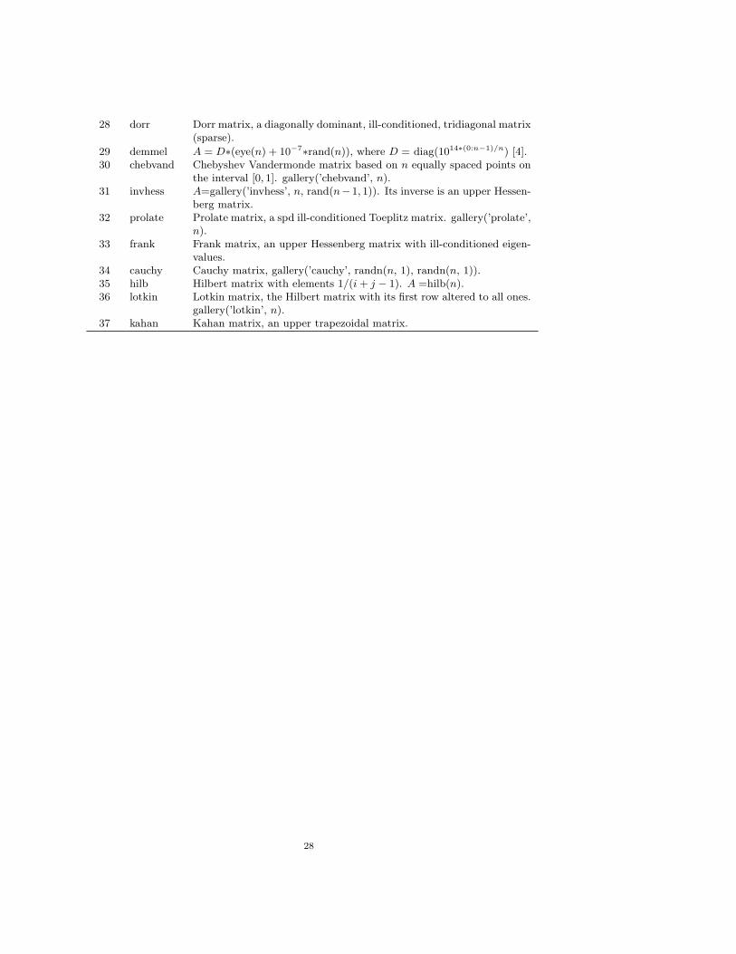


![Introduction to communication avoiding algorithms for ... · LU factorization is introduced in [40, 41], while the communication avoiding QR factorization is introduced in [24], and](https://static.documents.pub/doc/80x56/5ed73c06d37f9f58ca6a850c/introduction-to-communication-avoiding-algorithms-for-lu-factorization-is-introduced.jpg)


