Advanced Transport Phenomena The term "transport phenomena" describes the fundamental processes of momentum, energy, and mass transfer. This text provides a thorough discussion of transport phenomena, laying the foundation for understanding a wide variety of operations used by engineers. The book is arranged in three parallel parts covering the major topics of momentum, energy, and mass transfer. Each part begins with the theory, followed by illustrations of the way the theory can be used to obtain fairly complete solutions, and concludes with the four most common types of averaging used to obtain approximate solutions. A broad range of technologically important examples, as well as numerous exercises, are provided throughout the text. Based on the author's extensive teaching experience, a suggested lecture outline is also included. This book is intended for first-year graduate engineering students; it will be an equally useful reference for researchers in this field. John C. Slattery is the Jack E. and Frances Brown Chair of Engineering at Texas A&M University.
Transcript
Advanced Transport Phenomena
The term "transport phenomena" describes the fundamental processes of momentum, energy,and mass transfer. This text provides a thorough discussion of transport phenomena, layingthe foundation for understanding a wide variety of operations used by engineers.
The book is arranged in three parallel parts covering the major topics of momentum,energy, and mass transfer. Each part begins with the theory, followed by illustrations of theway the theory can be used to obtain fairly complete solutions, and concludes with the fourmost common types of averaging used to obtain approximate solutions. A broad range oftechnologically important examples, as well as numerous exercises, are provided throughoutthe text. Based on the author's extensive teaching experience, a suggested lecture outline isalso included.
This book is intended for first-year graduate engineering students; it will be an equallyuseful reference for researchers in this field.
John C. Slattery is the Jack E. and Frances Brown Chair of Engineering at Texas A&MUniversity.
C A M B R I D G E S E R I E S I N C H E M I C A L E N G I N E E R I N G
Editor
Arvind Varma, University of Notre Dame
Editorial Board
Alexis T. Bell, University of California, Berkeley
John Bridgwater, University of Cambridge
L. Gary Leal, University of California, Santa Barbara
Massimo Morbidelli, Swiss Federal Institute of Technology, Zurich
Stanley I. Sandier, University of Delaware
Michael L. Schuler, Cornell University
Arthur W. Westerberg, Carnegie Mellon University
Books in the Series
E. L. Cussler, Diffusion: Mass Transfer in Fluid Systems, second edition
Liang-Shih Fan and Chao Zhu, Principles of Gas-Solid Flows
Hasan Orbey and Stanley I. Sandier, Modeling Vapor-Liquid Equilibria:
Cubic Equations of State and Their Mixing Rules
T. Michael Duncan and Jeffrey A. Reimer, Chemical Engineering Design
and Analysis: An Introduction
John C. Slattery, Advanced Transport Phenomena
A. Varma, M. Morbidelli and H. Wu, Parametric Sensitivity
in Chemical Systems
Advanced TransportPhenomena
John C. Slattery
CAMBRIDGEUNIVERSITY PRESS
cambridge university press Cambridge, New York, Melbourne, Madrid, Cape Town, Singapore,
São Paulo, Delhi, Dubai, Tokyo, Mexico City
Cambridge University Press32 Avenue of the Americas, New York ny 10013-2473, USA
www.cambridge.orgInformation on this title: www.cambridge.org/9780521635653
This publication is in copyright. Subject to statutory exceptionand to the provisions of relevant collective licensing agreements,no reproduction of any part may take place without the written
permission of Cambridge University Press.
First published 1999Reprinted 2005
A catalogue record for this publication is available from the British Library.
Library of Congress Cataloguing in Publication Data Slattery, John Charles, 1932—
Advanced transport phenomena / John C. Slattery.p. m. — (Cambridge series in chemical engineering)
ISBN 0-521-63203-x (hb). — ISBN 0-521-63565-9 (pb)1. Transport theory. 2. Chemical engineering. I. Title.
II. Series.TP156.T7S57 1999
660´.2842 —dc21 98-44872 CIP
isbn 978-0-521-63203-4 Hardbackisbn 978-0-521-63565-3 Paperback
Cambridge University Press has no responsibility for the persistence oraccuracy of URLs for external or third-party internet websites referred to in
this publication, and does not guarantee that any content on such websites is,or will remain, accurate or appropriate. Information regarding prices, travel
timetables, and other factual information given in this work is correct atthe time of first printing but Cambridge University Press does not guarantee
the accuracy of such information thereafter.
Contents
PrefaceList of Notation
I Kinematics1.1 Motion1.2 Frame
1.2.11.2.2
1.3 Mass1.3.11.3.21.3.31.3.41.3.51.3.61.3.7
Changes of FrameEquivalent Motions
Conservation of MassTransport TheoremDifferential Mass BalancePhase InterfaceTransport Theorem for a Region Containing a Dividing SurfaceJump Mass Balance for Phase InterfaceStream Functions
page xvxix
1199151818182123232526
Foundations for Momentum Transfer2.1 Force2.2 Additional Postulates
2.2.1 Momentum and Moment of Momentum Balances2.2.2 Stress Tensor2.2.3 Differential and Jump Momentum Balances2.2.4 Symmetry of Stress Tensor
2.3 Behavior of Materials2.3.1 Some General Principles2.3.2 Simple Constitutive Equation for Stress2.3.3 Generalized Newtonian Fluid2.3.4 Noll Simple Fluid
2.4 Summary2.4.1 Differential Mass and Momentum Balances2.4.2 Stream Function and the Navier-Stokes Equation
282830303233353737394348505055
2.4.3 Interfacial Tension and the Jump Mass and Momentum Balances 58
Contents
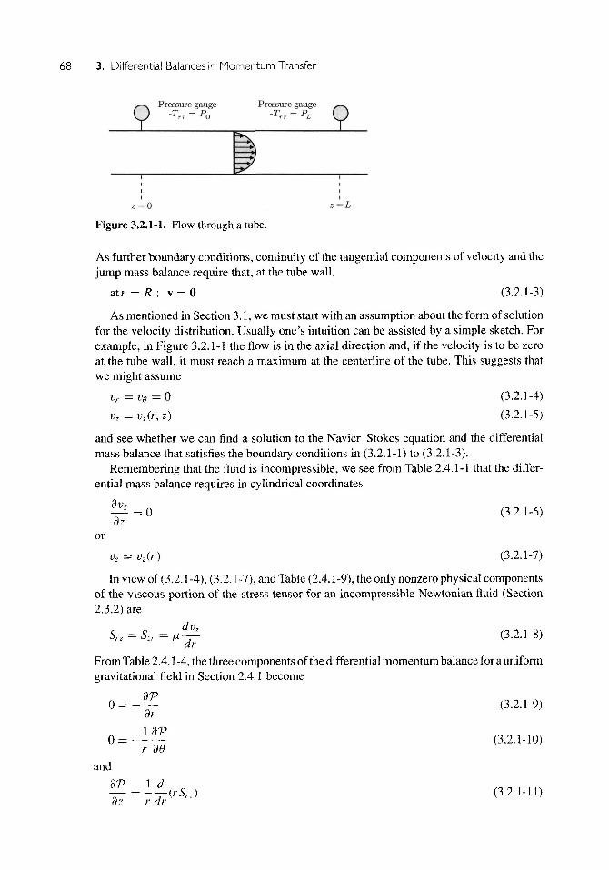
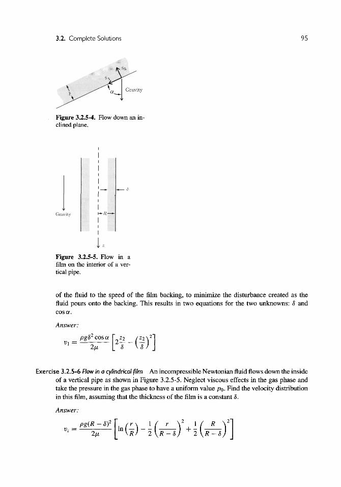
3 Differential Balances in Momentum Transfer 653.1 Philosophy 663.2 Complete Solutions 67
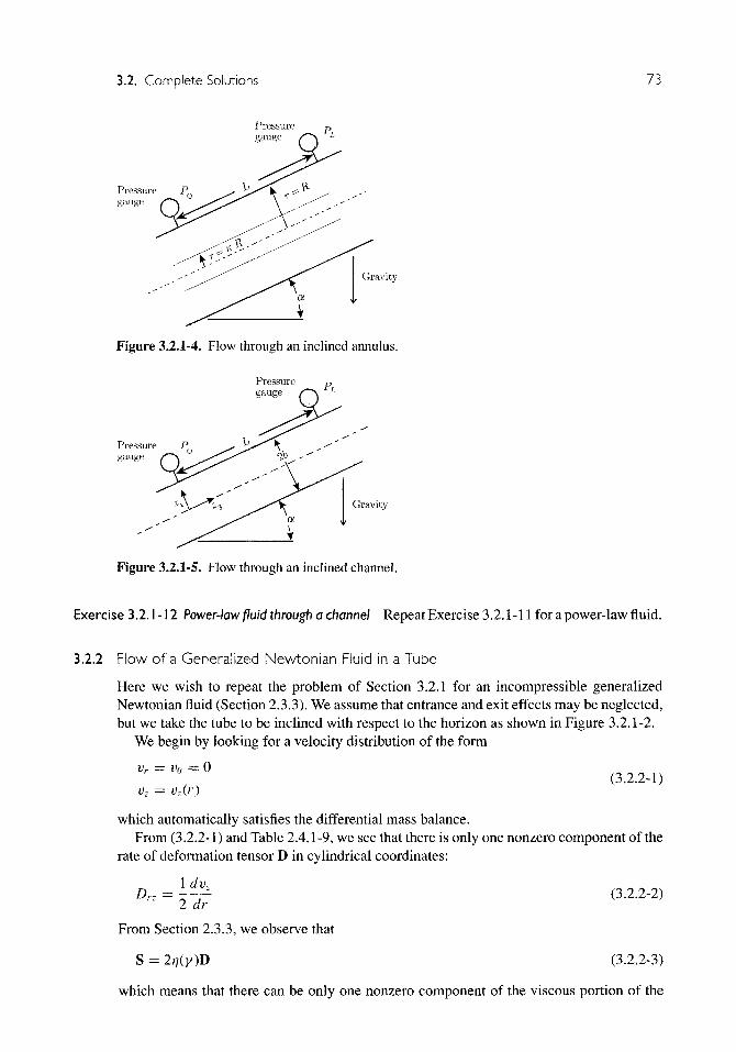
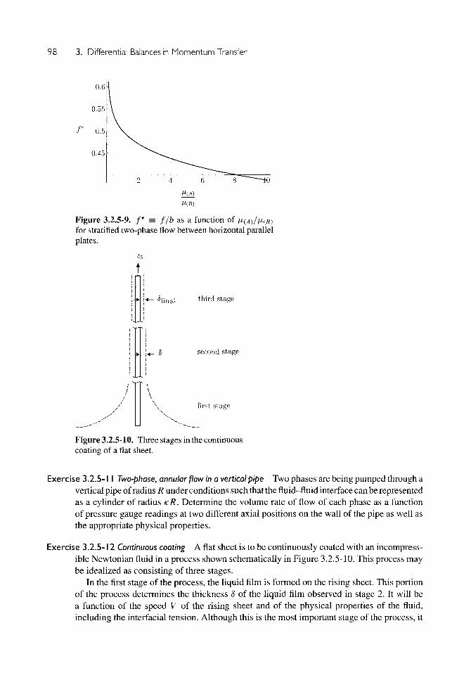
3.2.1 Flow in a Tube 673.2.2 Flow of a Generalized Newtonian Fluid in a Tube 733.2.3 Tangential Annular Flow 783.2.4 Wall That Is Suddenly Set in Motion 843.2.5 Rotating Meniscus 90
3.3 Creeping Flows 993.3.1 Flow in a Cone—Plate Viscometer 1013.3.2 Flow Past a Sphere 1113.3.3 Thin Draining Films 1163.3.4 Melt Spinning 121
3.4 Nonviscous Flows 1313.4.1 Bernoulli Equation 1333.4.2 Potential Flow Past a Sphere 1363.4.3 Plane Potential Flow in a Corner 140
3.5 Boundary-Layer Theory 1433.5.1 Plane Flow Past a Flat Plate 1433.5.2 More on Plane Flow Past a Flat Plate 1483.5.3 Plane Flow Past a Curved Wall 1533.5.4 Solutions Found by Combination of Variables 1583.5.5 Flow in a Convergent Channel 1623.5.6 Flow Past a Body of Revolution 165
3.6 Stability 1723.6.1 Stability of a Liquid Thread 174
4 Integral Averaging in Momentum Transfer 1824.1 Time Averaging 182
4.1.1 Time Averages 1834.1.2 The Time Average of a Time-Averaged Variable 1854.1.3 Empirical Correlations for T w 1864.1.4 Wall Turbulence in Flow Through a Tube 190
4.2 Area Averaging 1944.2.1 Flow from Rest in a Circular Tube 195
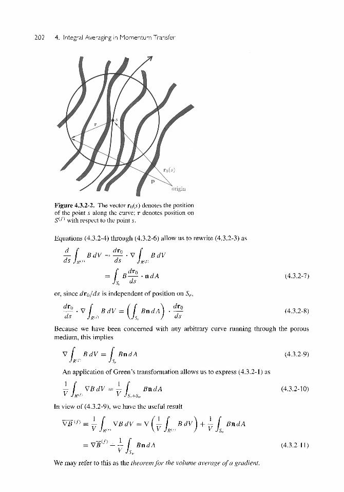
4.3 Local Volume Averaging 1974.3.1 The Concept 1984.3.2 Theorem for the Local Volume Average of a Gradient 2004.3.3 The Local Volume Average of the Differential Mass Balance 2034.3.4 The Local Volume Average of the Differential
Momentum Balance 2034.3.5 Empirical Correlations for g 2054.3.6 Summary of Results for an Incompressible Newtonian Fluid 2094.3.7 Averages of Volume-Averaged Variables 2104.3.8 Flow through a Packed Tube 2114.3.9 Neglecting the Divergence of the Local Volume-Averaged
Extra Stress 215
Contents ix
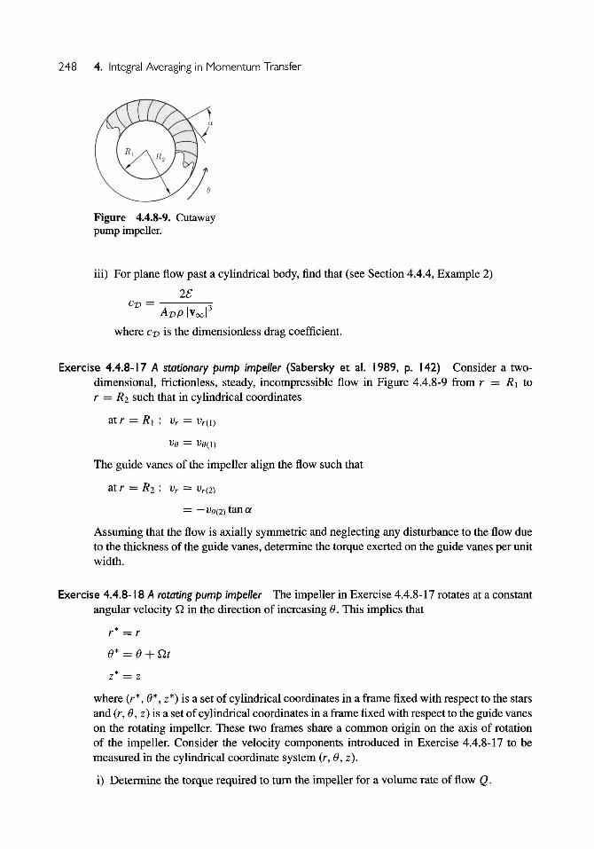
4.4 Integral Balances 2174.4.1 The Integral Mass Balance 2184.4.2 The Integral Mass Balance for Turbulent Flows 2204.4.3 The Integral Momentum Balance 2224.4.4 Empirical Correlations for T and Q 2254.4.5 The Mechanical Energy Balance 2294.4.6 Empirical Correlations for S 2344.4.7 Integral Moment-of-Momentum Balance 2364.4.8 Examples 239
5 Foundations for Energy Transfer 2505.1 Energy 250
5.1.1 Energy Balance 2505.1.2 Radiant and Contact Energy Transmission 2515.1.3 Differential and Jump Energy Balances 253
5.2 Entropy 2565.2.1 Entropy Inequality 2565.2.2 Radiant and Contact Entropy Transmission 2575.2.3 The Differential and Jump Entropy Inequalities 259
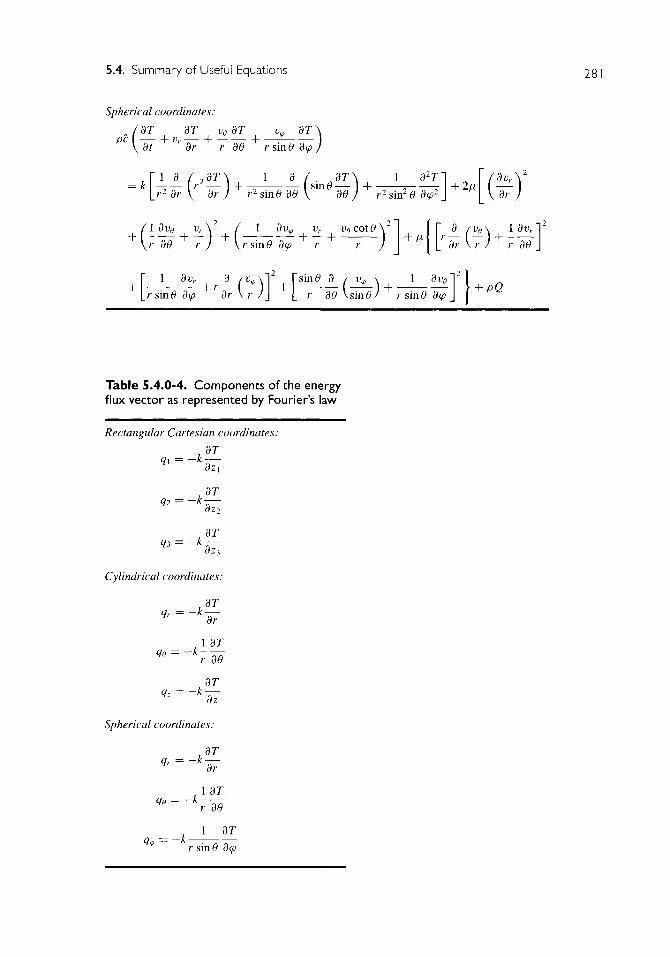
5.3 Behavior of Materials 2615.3.1 Implications of the Differential Entropy Inequality 2615.3.2 Restrictions on Caloric Equation of State 2705.3.3 Energy and Thermal Energy Flux Vectors 2735.3.4 Stress Tensor 275
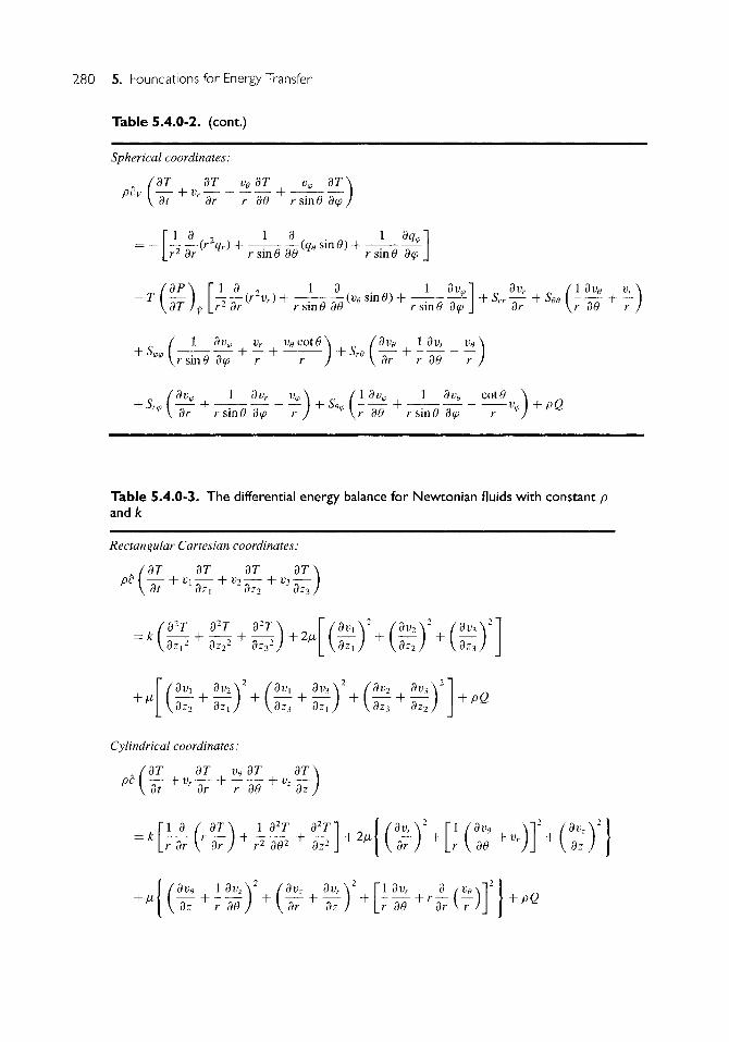
5.4 Summary of Useful Equations 277
6 Differential Balances in Energy Transfer 2836.1 Philosophy 2836.2 Conduction 284
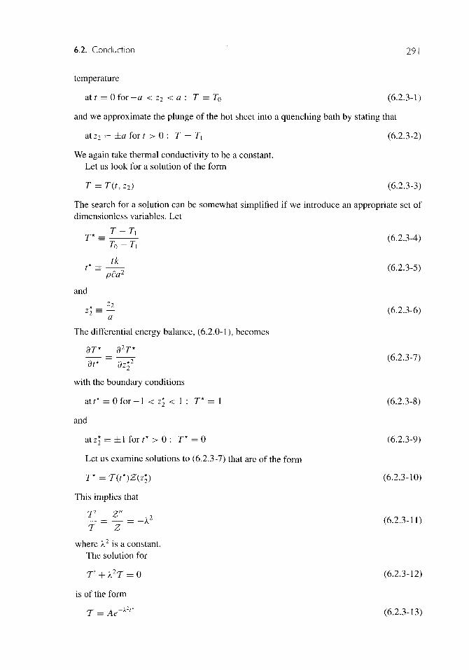
6.2.1 Cooling of a Semi-Infinite Slab: Constant Surface Temperature 2856.2.2 Cooling a Semi-Infinite Slab: Newton's "Law" of Cooling 2876.2.3 Cooling a Flat Sheet: Constant Surface Temperature 290
6.3 More Complete Solutions 2946.3.1 Couette Flow of a Compressible Newtonian Fluid 2946.3.2 Couette Flow of a Compressible Newtonian Fluid with Variable
Viscosity and Thermal Conductivity 3026.3.3 Rate at Which a Fluid Freezes (or a Solid Melts) 309
6.4 When Viscous Dissipation Is Neglected 3146.4.1 Natural Convection 316
6.5 No Convection 3246.6 No Conduction 326
6.6.1 Speed of Propagation of Sound Waves 3276.7 Boundary-Layer Theory 331
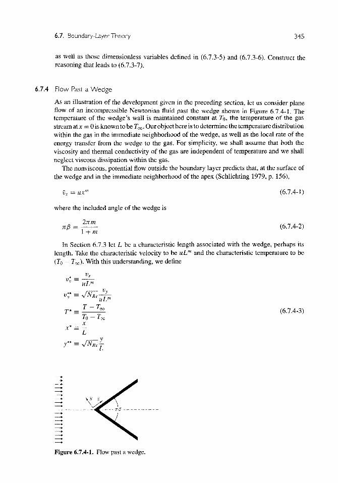
6.7.1 Plane Flow Past a Flat Plate 3316.7.2 More on Plane Flow Past a Flat Plate 3356.7.3 Plane Flow Past a Curved Wall 3426.7.4 Flow Past a Wedge 345
Contents
6.7.5 Flow Past a Body of Revolution 3496.7.6 Energy Transfer in the Entrance of a Heated Section of a Tube 3516.7.7 More on Melt Spinning 359
6.8 More About Energy Transfer in a Heated Section of a Tube 3616.8.1 Constant Temperature at Wall 3626.8.2 Constant Energy Flux at Wall 366
7 Integral Averaging in Energy Transfer 3747.1 Time Averaging 374
7.1.1 The Time-Averaged Differential Energy Balance 3747.1.2 Empirical Correlation for the Turbulent Energy Flux 3757.1.3 Turbulent Energy Transfer in a Heated Section of a Tube 378
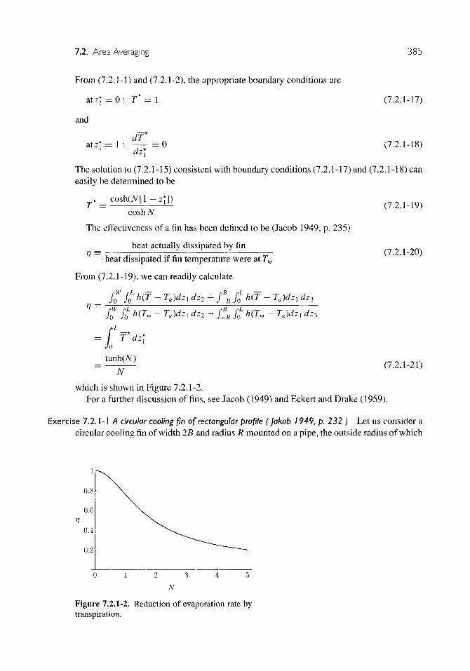
7.2 Area Averaging 3827.2.1 A Straight Cooling Fin of Rectangular Profile 383
7.3 Local Volume Averaging 3867.3.1 The Local Volume Average of the Differential Energy Balance 3877.3.2 Empirical Correlations for h 3897.3.3 Summary of Results for a Nonoriented,
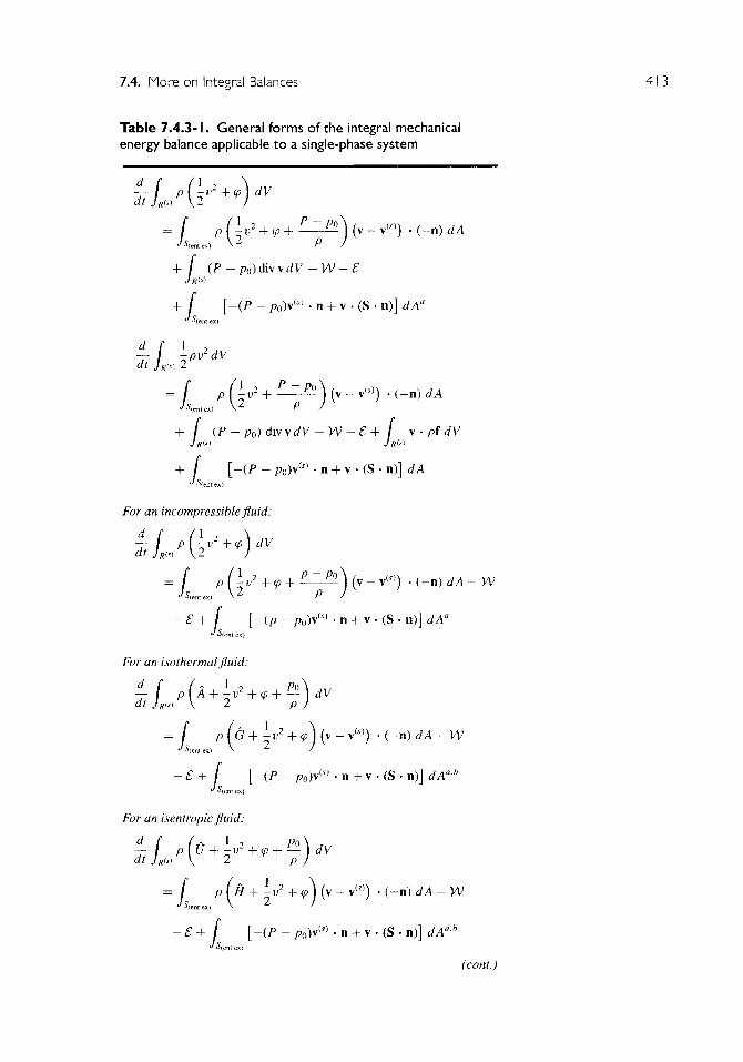
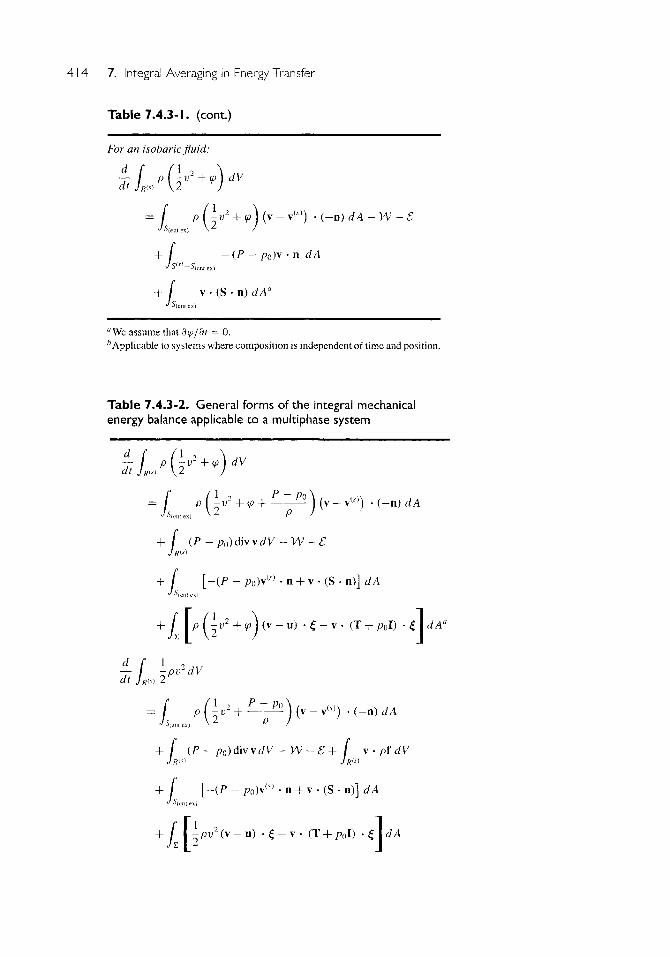
7.4 More on Integral Balances 3997.4.1 The Integral Energy Balance 3997.4.2 Empirical Correlations for Q 4077.4.3 More About the Mechanical Energy Balance 4107.4.4 The Integral Entropy Inequality 4177.4.5 Integral Entropy Inequality for Turbulent Flows 4187.4.6 Example 418
8 Foundations for Mass Transfer 4238.1 Viewpoint 423
8.1.1 Body, Motion, and Material Coordinates 4248.2 Species Mass Balance 426
8.2.1 Differential and Jump Balances 4268.2.2 Concentration, Velocities, and Mass Fluxes 428
8.3 Revised Postulates 4308.3.1 Conservation of Mass 4328.3.2 Momentum Balance 4338.3.3 Moment of Momentum Balance 4348.3.4 Energy Balance 4358.3.5 Entropy Inequality 435
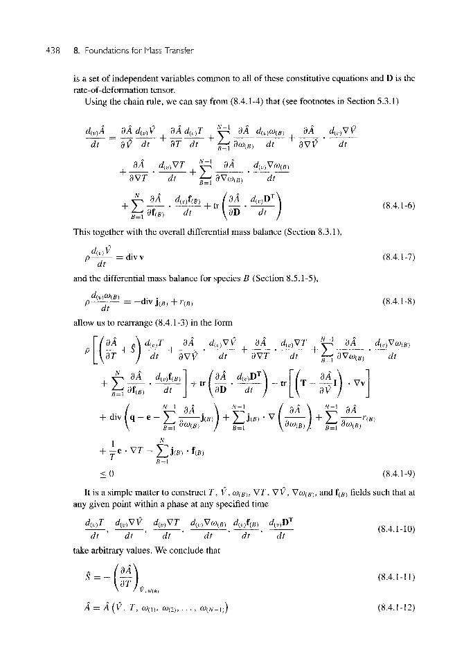
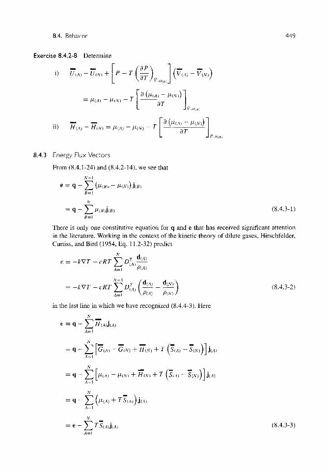
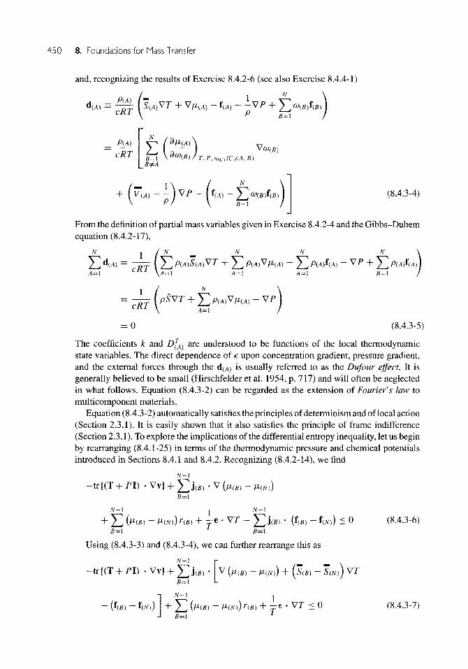
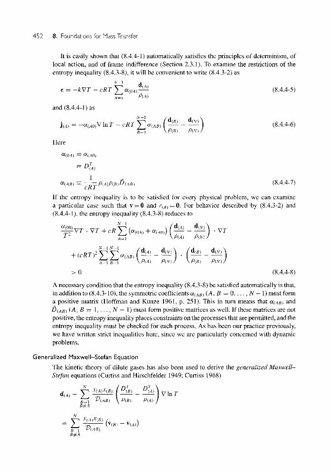
8.4 Behavior 4368.4.1 Implications of the Differential Entropy Inequality 4378.4.2 Restrictions on Caloric Equation of State 4428.4.3 Energy Flux Vectors 4498.4.4 Mass Flux Vector 4518.4.5 Mass Flux Vector in Binary Solutions 4598.4.6 Mass Flux Vector: Limiting Cases in Ideal Solutions 462
Contents xi
8.4.7 Constitutive Equations for the Stress Tensor 4648.4.8 Rates of Reactions 464
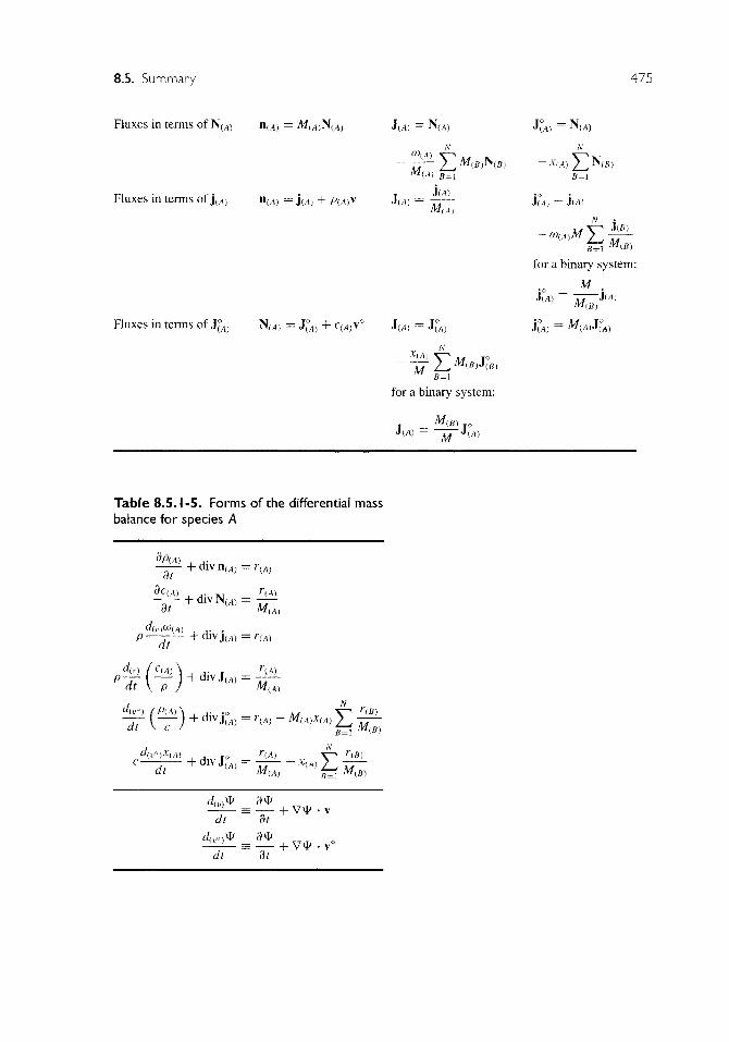
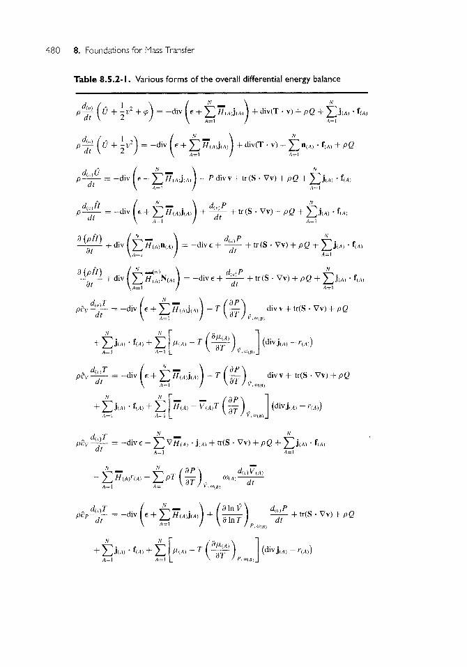
8.5 Summary 4728.5.1 Summary of Useful Equations for Mass Transfer 4728.5.2 Summary of Useful Equations for Energy Transfer 477
9 Differential Balances in Mass Transfer 4829.1 Philosophy of Solving Mass-Transfer Problems 4829.2 Energy and Mass Transfer Analogy 483
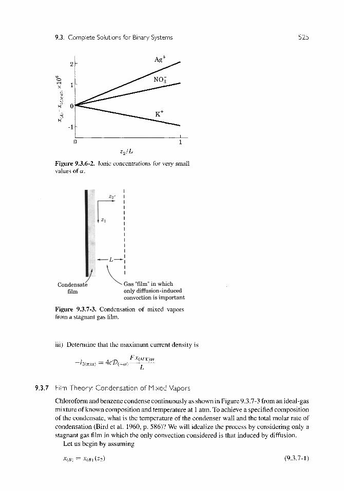
9.2.1 Film Theory 4859.3 Complete Solutions for Binary Systems 488
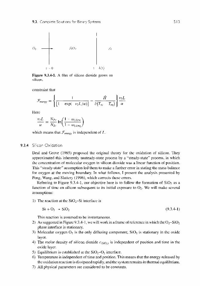
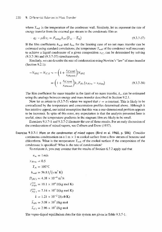
9.3.1 Unsteady-State Evaporation 4899.3.2 Rate of Isothermal Crystallization 5019.3.3 Rate of Nonisothermal Crystallization 5079.3.4 Silicon Oxidation 5139.3.5 Pressure Diffusion in a Natural Gas Well 5159.3.6 Forced Diffusion in Electrochemical Systems 5209.3.7 Film Theory: Condensation of Mixed Vapors 5259.3.8 Two- and Three-Dimensional Problems 532
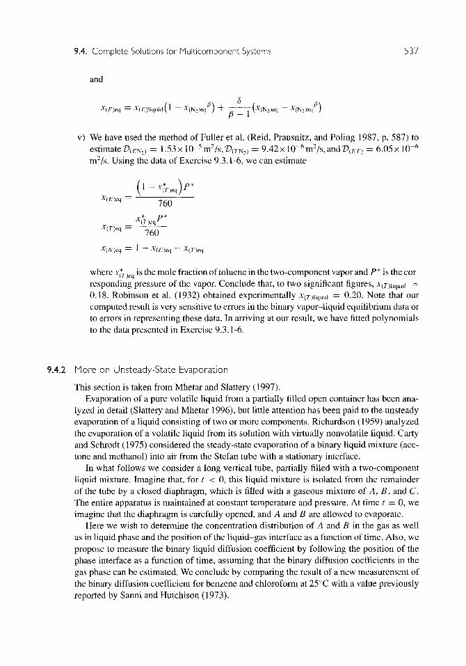
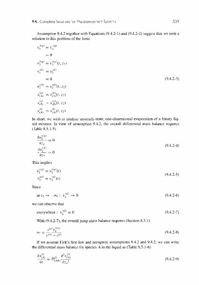
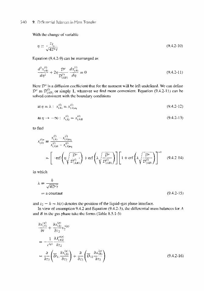
9.4 Complete Solutions for Multicomponent Systems 5339.4.1 Film Theory: Steady-State Evaporation 5339.4.2 More on Unsteady-State Evaporation 5379.4.3 Oxidation of Iron 545
9.5 Boundary-Layer Theory 5579.5.1 Plane Flow Past a Flat Plate 5589.5.2 Flow Past Curved Walls and Bodies of Revolution 561
9.6 Forced Convection in Dilute Solutions 5619.6.1 Unsteady-State Diffusion with a First-Order
Homogeneous Reaction 5629.6.2 Gas Absorption in a Falling Film with Chemical Reaction 566
10 Integral Averaging in Mass Transfer 57310.1 Time Averaging 573
10.1.1 The Time-Averaged Differential Mass Balance for Species A 57310.1.2 Empirical Correlations for the Turbulent Mass Flux 57510.1.3 Turbulent Diffusion from a Point Source in a Moving Stream 576
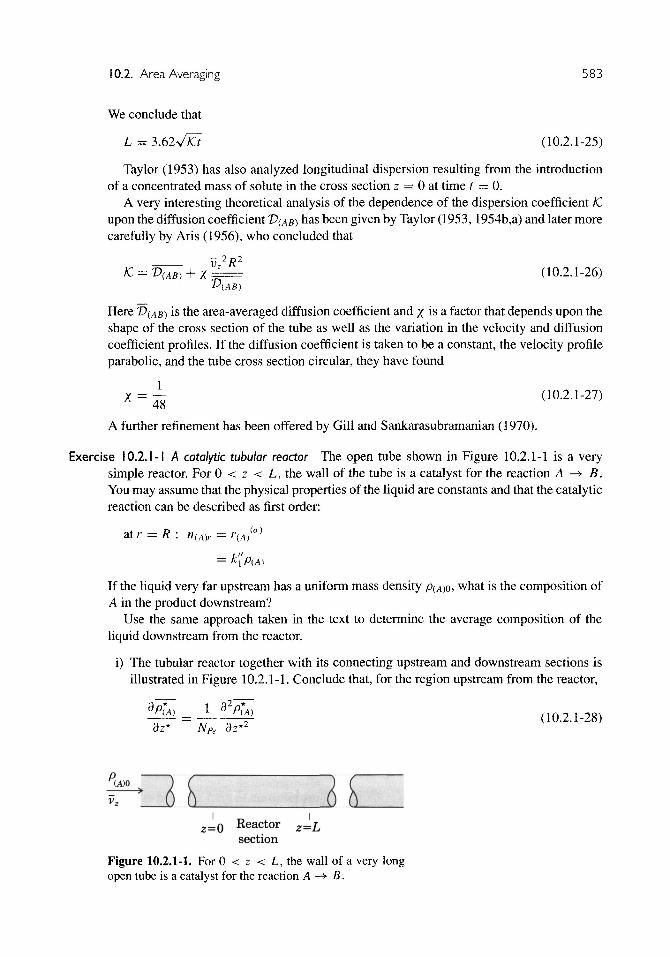
10.2 Area Averaging 58010.2.1 Longitudinal Dispersion 580
10.3 Local Volume Averaging 58510.3.1 Local Volume Average of the Differential Mass Balance
for Species A 58510.3.2 When Fick's First Law Applies 58610.3.3 Empirical Correlations for Tortuosity Vectors 58810.3.4 Summary of Results for a Liquid or Dense Gas in a
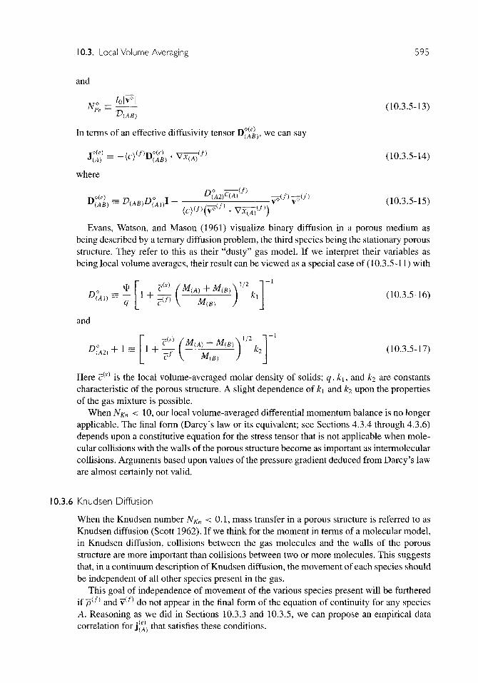
Nonoriented, Uniform-Porosity Structure 59210.3.5 When Fick's First Law Does Not Apply 59310.3.6 Knudsen Diffusion 595
xii Contents
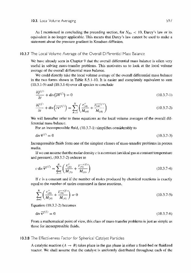
10.3.7 The Local Volume Average of the Overall DifferentialMass Balance 597
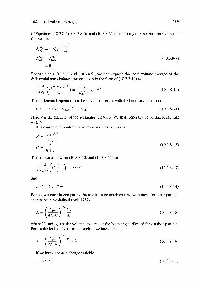
10.3.8 The Effectiveness Factor for Spherical Catalyst Particles 59710.4 Still More on Integral Balances 603
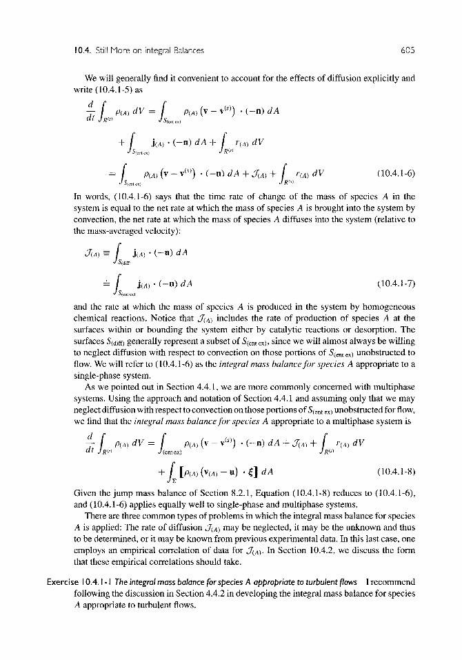
10.4.1 The Integral Mass Balance for Species A 60410.4.2 Empirical Correlations for J^ 60610.4.3 The Integral Overall Balances 60910.4.4 Example 614
Tensor Analysis 619A.I Spatial Vectors 619
A.I.I Definition** 619A.1.2 Position Vectors 621A.1.3 Spatial Vector Fields 621A.1.4 Basis 622A.1.5 Basis for the Spatial Vector Fields 624A.1.6 Basis for the Spatial Vectors 625A.1.7 Summation Convention 626
A.2 Determinant 627A.2.1 Definitions 627
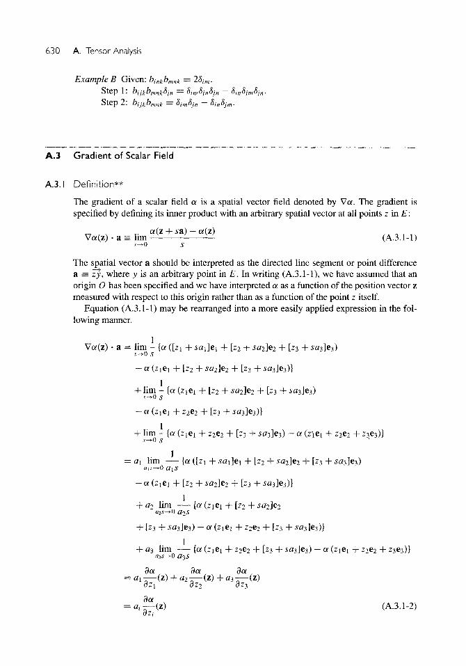
A.3 Gradient of Scalar Field 630A.3.1 Definition** 630
A.5 Second-Order Tensors 644A.5.1 Components of Second-Order Tensor Fields 645A.5.2 Transpose of a Second-Order Tensor Field** 650A.5.3 Inverse of a Second-Order Tensor Field 654A.5.4 Trace of a Second-Order Tensor Field** 655
A.6 Gradient of Vector Field 657A.6.1 Definition** 657A.6.2 Covariant Differentiation* 658
A.7 Third-Order Tensors 664A.7.1 Definition 664A.7.2 Components of Third-Order Tensor Fields 665A.7.3 Another View of Third-Order Tensor Fields 668
A.8 Gradient of Second-Order Tensor Field 669A.8.1 Definition 669A.8.2 More on Covariant Differentiation* 670
A.9 Vector Product and Curl 673A.9.1 Definitions** 673A.9.2 More on the Vector Product and Curl 674
A.10 Determinant of Second-Order Tensor 677A.10.1 Definition 677
Contents xiii
A. 11 Integration 679A.l l . l Spatial Vector Fields** 679A.11.2 Green's Transformation 680A.11.3 Change of Variable in Volume Integrations** 683
B More on the Transport Theorem 685
References 687Author!Editor Index 699Index 703
Preface
Transport phenomena is the term popularized, if not coined, by Bird, Stewart, and Lightfoot(1960) to describe momentum, energy, and mass transfer. This book is based upon roughlythirty-five years of teaching first-year graduate students, first at Northwestern Universityand later at Texas A&M University. It draws upon Momentum, Energy, and Mass Transferin Continua (Slattery 1981), the first edition of which was written at an early stage of mycareer, as well as Interfacial Transport Phenomena (Slattery 1990), which is intended for amuch more specialized audience.
As you examine the table of contents, you will observe that, superimposed upon the threemajor themes of momentum, energy, and mass transfer, there are three minor themes. I begineach of these blocks of material with a discussion of the theory that we are to use: Chapters1, 2, 5, and 8. This is followed by illustrations of the various ways in which the theory canbe used to obtain fairly complete solutions: Chapters 3, 6, and 9. Finally, I conclude byexamining the four most common types of averaging that are used to obtain approximatesolutions: Chapters 4, 7, and 10.
This book is intended both as a textbook for first-year graduate students and as a self-studytext for students and researchers interested in the field. The book is relatively long, in orderto accommodate a variety of course syllabi as well as a range of self-study interests.
In spite of its length, you easily will find topics that I have left out. For example, I couldhave included more on the mathematical techniques that are used in solving various transportphenomena problems. Recognizing that mathematics is the language most naturally used toexplain transport phenomena, I have included an appendix outlining tensor analysis. But theprimary purpose of this text is to discuss transport phenomena, not mathematics.
In this context, I encourage my students to use software such as Mathematica (1996). Ihave found its symbolic capabilities particularly useful in doing perturbation analyses. Moregenerally, I have employed it in developing numerical solutions of transcendental equationsand nonlinear ordinary differential equations. Continuing with the concept that the primarypurpose of this text is to discuss transport phenomena, I have not included as part of the textthe details of my Mathematica notebooks.
In the lecture outline that follows, you will notice that I do not cover the entire book inmy own lectures. Nor do I begin with Appendix A before proceeding to Chapters 1 and 2.Although it sounds sensible to begin with a thorough grounding in the fundamentals of tensoranalysis, my experience is that this is relatively difficult for students. They don't understand
xvi Preface
initially why all of the mathematical apparatus is required. Instead, I begin with Chapters1 and 2, referring back to Appendix A as the various ideas are needed. For example, it ismuch easier to introduce students to (second-order) tensors when they understand why thisstructure is required.
On a more personal note, I would like to express my gratitude to the many graduatestudents with whom I have discussed this material both at Northwestern University and atTexas A&M University. I have listened to your questions and comments, and I have donemy best to take them into account. I am particularly grateful to a smaller group of activiststudents at both universities, my own students as well as the students of others, who havehelped me develop new material for the book. There are too many to name here, but I havedone my best to reference your papers and your suggestions in the text. You have madeteaching exciting.
Special thanks are due to Professor Pierce Cantrell (Department of Electrical Engineering,Texas A&M University) who made this book possible. He suggested that I use KIpX, built abigger version on his faster machine, created special symbols, showed me how to introducecomputer modern fonts in the figures, and installed a high-speed link between my home andmy office.
Finally, I would also like to thank Christine Sanchez, who assisted me in converting mynotes to MgX, Peter Weiss, who created many of the drawings, and Professor Nelson H. F.Beebe, who allowed me to use a prepublication version of his author index (Beebe 1998)for KTpX.
May 12,1997
Sample Lecture Outline
What follows is a sample outline for 28 weeks of lectures (three hours per week of lecturesand at least one hour per week of problem discussion) over two semesters. There is somechange from year to year for several reasons. I attempt to adjust the pace of the class tothe response of the students. In discussing Chapters 3, 6, and 9 /1 usually base my lectureson exercises rather than the examples worked out in the text. Finally, I am always lookingfor new material. Some instructors will wish to consider problems resulting in numericalsolution of partial differential equations as software appropriate for a busy class becomesavailable.
In examining this outline, keep in mind that I do not cover all sections with the sameintensity. In some cases, I am trying to emphasize only the concept and not the details. Inother cases, my students may have seen similar material in other classes.
Preface xvii
First Semester
W e e k Tentative reading ass ignment
1 Introduction, 1.1, 1.3.1, 1.3.2, Appendix B2 1.3.3 through 1.3.7, A. 1.1 through A. 1.7, A.2.1, A.3.1, A.4.13 Chapter 2 through 2.2.3, A.5.1 through A.5.4, A.6.1, A.8.1, A.I 1.1, A.I 1.24 2.2.4, 2.3.1 through 2.3.35 3.1, 3.2.1, first exam6 3.2.2,3.2.37 3.2.48 3.2.59 3.3 through 3.3.1, second exam10 3.3.4,3.4.111 3.4.2,3.4.312 3.5.1,3.5.2, third exam13 3.5.3 through 3.5.614 3.6.1
Second semester
Week
1234567891011121314
Tentative reading assignment
5.1.1 through 5.1.35.2.1 through 5.4.1, 6.1, 6.2 through 6.2.36.3 through 6.3.16.3.26.3.3,6.4.16.5.1, 6.6 through 6.6.1, 6.7.1, first exam6.7.2 through 6.7.6, 6.8.1, 6.8.28.2.1,8.2.2,8.3,8.4,9.29.3.19.3.29.3.3, 9.3.49.3.6, 9.3.7, second exam9.4.1,9.4.29.4.3
List of Notation
Relative activity on a mass basis of species A defined by (8.4.5-5).a^ Relative activity on a molar basis of species A defined in Exercise 8.4.4-1.
A Helmholtz free energy per unit mass. See, for example, Exercises 5.3.2-2 and8.4.2-2.
A Angular velocity tensor of starred frame with respect to unstarred frame definedby (1.2.2-8).
c Total molar density defined in Table 8.5.1-1.c Heat capacity per unit mass for an incompressible material.C(A) Molar density of species A, in moles per unit volume.cp Heat capacity per unit mass at constant pressure defined in Exercises 5.3.2-4
and 8.4.2-7.dy Heat capacity per unit mass at constant volume defined in Exercises 5.3.2-4 and
8.4.2-7.C, Right relative Cauchy-Green strain tensor defined by (2.3.4-3).C(AB) Defined by (8.4.4-23)d(A) Defined by (8.4.3-4).D Rate of deformation tensor defined by (2.3.2-3).*D(AB) Maxwell-Stefan diffusion coefficient introduced in (8.4.4-9). For dilute gas
mixtures, this is known as the binary diffusion coefficient.VQ{AB) Defined in Table 8.5.1-7D(AB) Curtiss diffusion coefficient defined in (8.4.4-1)D(AB) Defined by (8.4.4-18)dA Indicates that a surface integration is to be performed.dV Indicates that a volume integration is to be performed.e Thermal energy flux vector introduced in (5.2.3-5) and (8.3.5-4). See also
(5.3.1-25) and (8.4.1-24).e/ Rectangular Cartesian basis vector introduced in Section A. 1.5.f Sum of the external and mutual body force per unit mass. See the introduction
to Section 2.1.f(A> External or mutual force acting on species A.F Deformation gradient introduced in Exercise 2.3.2-1.Fr Relative deformation gradient introduced in (2.3.4-2).
xx List of Notation
g Acceleration of gravity. Also see Exercises A.4.1-4 and A.4.1-5.gij Defined by (A.4.1-10).gij Defined by (A.4.2-2) and (A.4.2-5).gz Defined by (A.4.1-4).G Gibbs free energy per unit mass. See, for example, Exercises 5.3.2-2 and 8.4.2-2.H Mean curvature. See Tables 2.4.3-1 through 2.4.3-8.H Enthalpy per unit mass. See, for example, Exercises 5.3.2-2 and 8.4.2-2.j(4) Mass flux relative to v as defined in Table 8.5.1-4.'f(A) Mass flux relative to v° as defined in Table 8.5.1-4.J(4) Molar flux relative to v as defined in Table 8.5.1-4.J^j Molar flux relative to v° as defined in Table 8.5.1-4.M Molar-averaged molecular weight defined in Table 8.5.1-1.M(A) Molecular weight of species A .n Outwardly directed unit normal to a closed surface.ik(A) Mass flux of species A relative to a fixed frame of reference as defined in Table
8.5.1-4.N(A) Molar flux of species A relative to a fixed frame of reference as defined in Table
8.5.1-4.NBr Brinkman number as in (6.4.0-5).NDa Damkohler number as in Exercise 9.6.2-10.Nfr Froude number as in (6.4.0-5).N%n Knudsen number as in (10.3.2-1).NPe Peclet number as in (6.4.0-5).NPeM Peclet number for mass transfer as in (9.2.0-8).Npr Prandtl number as in (6.4.0-5).NRe Reynolds number as in (6.4.0-5).NRu Ruark number as in (6.4.0-5).NSc Schmidt number as in (9.2.0-8).NSt Strouhal number as in (6.4.0-5).p Mean pressure defined by (2.3.2-26).p Position vector introduced in Section A. 1.2.P Thermodynamic pressure. See (2.3.2-21), (5.3.1-30), and (8.4.1-28).V Modified pressure for an incompressible fluid defined by (2.4.1-5).q Energy flux vector introduced in (5.1.3-5).Q Sum of the external and mutual energy transmission rates per unit mass. See
Section 5.1.2.Q Time-dependent orthogonal transformation introduced in Section 1.2.1.r Cylindrical coordinate introduced in Exercise A.4.1 -4 and spherical coordinate
introduced in Exercise A.4.1-5.r(/t) Rate of production of species A per unit volume by homogeneous chemical
reactions.rfy Rate of production of species A per unit area by heterogeneous chemical reac-
tions.R Gas law constant. Also used as the radius of a tube or sphere.R(m) Region occupied by a material body.S Entropy per unit mass.S Extra stress or viscous portion of the stress tensor defined by (2.3.2-27) for an
incompressible fluid and by (5.3.1-27) or (8.4.1-26) for a compressible fluid.
List of Notation xxi
S(m) Closed surface bounding a material body.t Time.t Stress vector, in force per unit area.T Temperature introduced in (5.2.3-5) and (8.3.5-4).T Stress tensor introduced in Section 2.2.2.u Velocity of a point on the dividing surface as introduced in Section 1.3.5.U(A) Velocity of species A relative to v defined in Table 8.5.1-3.U(A) Velocity of species A relative to v° defined in Table 8.5.1-3.U Internal energy per unit mass introduced in Section 5.1.1.v Velocity defined by (1.1.0-13); also mass-averaged velocity defined in Table
8.5.1-3.v° Molar-averaged velocity defined in Table 8.5.1-3.\{A) Velocity of species A defined by (8.1.1-9).X(A) Mole fraction defined in Table 8.5.1-1.X(£ ) Configuration of body as introduced in Section 1.1.X~~l(z) Material particle whose place in E is z.z Point in E space introduced in Section A. 1.1 as well as cylindrical coordinate
introduced in Exercise A.4.1 -4.z, Rectangular Cartesian coordinate introduced in (A. 1.5-5).z Position vector for the point z introduced in Section A. 1.2.zKi Coordinate of zK in the reference configuration K.zK Position vector of a material particle in the reference configuration K .y Surface or interfacial tension introduced in (2.4.3-1)Y(A) Activity coefficient for species A defined by (8.4.8-9).e Defined by (8.4.3-4).£ Material particle introduced in Section 1.1.rj Apparent viscosity for an incompressible generalized Newtonian fluid intro-
duced in (2.3.3-1).0 Cylindrical coordinate introduced in Exercise A.4.1-4 as well as spherical co-
ordinate introduced in Exercise A.4.1-5.K Bulk viscosity of a Newtonian fluid defined by (2.3.2-24).K Reference configuration of body as introduced in Section 1.1.K~1(ZK) Material particle at the place zK as introduced in Section 1.1.\x Shear viscosity of a Newtonian fluid introduced in (2.3.2-21) as well as chemical
potential on a mass basis for a single-component material defined by (5.3.2-6).fi(A) Chemical potential for species A on a mass basis defined by (8.4.2-6).lj(m) Chemical potential on a molar basis for a single-component material defined by
(5.3.2-7).jU^ Chemical potential for species A on a molar basis defined by (8.4.2-7).£ Unit normal to a dividing surface. See Section 1.3.5 for sign convention. See
Tables 2.4.3-1 through 2.4.3-8 for specific examples, when using interfacialtension y.
p Mass density, in mass per unit volume; also total mass density defined in Table8.5.1-1.
p i A ) Mass density of species A, in mass per unit volume.£ Dividing surfaces within a material body.4> Gravitational potential introduced in (2.4.1-3).
xxii List of Notation
cp Spherical coordinate introduced in Exercise A.4.1-5 as well as the fluidity foran incompressible generalized Newtonian fluid introduced in (2.3.3-19).
X~l (z, t) Material particle at z and t., t) Motion of body as introduced in Section 1.1.&K , t) Defined by (1.1.0-9).
Stream function introduced in Section 1.3.7.Mass fraction of species A defined in Table 8.5.1-1.
u? Angular velocity vector of the unstarred frame with respect to the starred frameas defined by (1.2.2-11).
d{m)/dt Material derivative defined by (1.1.0-12).Indicates that the quantity is per unit mass.Indicates that the quantity is per unit volume.
2. Indicates that the quantity is per unit mole.0(4) Indicates that the quantity is a partial mass variable for species A as defined in_ Exercise 8.4.2-4.4>(
(™) Indicates that the quantity is a partial molar variable for species A as defined inExercise 8.4.2-5.
Defined by (1.3.5-5) as the jump of the quantity enclosed across an interface.
Advanced Transport Phenomena
Kinematics
THIS ENTIRE CHAPTER IS INTRODUCTORY in much the same way as Ap-pendix A is. In Appendix A, I introduce the mathematical language that I shall be using
in describing physical problems. In this chapter, I indicate some of the details involved in rep-resenting from the continuum point of view the motions and deformations of real materials.This chapter is important not only for the definitions introduced, but also for the viewpointtaken in some of the developments. For example, the various forms of the transport theoremwill be used repeatedly throughout the text in developing differential equations and integralbalances from our basic postulates.
Perhaps the most difficult point for a beginner is to properly distinguish between thecontinuum model for real materials and the particulate or molecular model. We can all agreethat the most factually detailed picture of real materials requires that they be represented interms of atoms and molecules. In this picture, mass is distributed discontinuously throughoutspace; mass is associated with the protons, neutrons, electrons,..., which are separated byrelatively large voids. In the continuum model for materials, mass is distributed continu-ously through space, with the exception of surfaces of discontinuity, which represent phaseinterfaces or shock waves.
The continuum model is less realistic than the particulate model but far simpler. For manypurposes, the detailed accuracy of the particulate model is unnecessary. To our sight andtouch, mass appears to be continuously distributed throughout the water that we drink and theair that we breathe. The problem is analogous to a study of traffic patterns on an expressway.The speed and spacings of the automobiles are important, but we probably should not worryabout whether the automobiles have four, six, or eight cylinders.
This is not to say that the particulate theories are of no importance. Information is lostin a continuum picture. It is only through the use of statistical mechanics that a complete apriori prediction about the behavior of the material can be made. I will say more about thisin the next chapter.
I.I Motion
My goal in this book is to lay the foundation for understanding a wide variety of operationsemployed in the chemical and petroleum industries. To be specific, consider the extrusion of
I. Kinematics
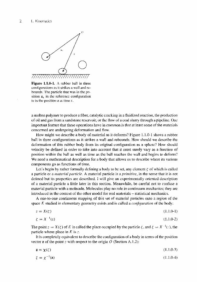
Figure 1.1.0-1. A rubber ball in threeconfigurations as it strikes a wall and re-bounds. The particle that was in the po-sition zK in the reference configurationis in the position z at time t.
a molten polymer to produce a fiber, catalytic cracking in a fluidized reaction, the productionof oil and gas from a sandstone reservoir, or the flow of a coal slurry through a pipeline. Oneimportant feature that these operations have in common is that at least some of the materialsconcerned are undergoing deformation and flow.
How might we describe a body of material as it deforms? Figure 1.1.0-1 shows a rubberball in three configurations as it strikes a wall and rebounds. How should we describe thedeformation of this rubber body from its original configuration as a sphere? How shouldvelocity be defined in order to take into account that it must surely vary as a function ofposition within the ball as well as time as the ball reaches the wall and begins to deform?We need a mathematical description for a body that allows us to describe where its variouscomponents go as functions of time.
Let's begin by rather formally defining a body to be set, any element £ of which is calleda particle or a material particle. A material particle is a primitive, in the sense that it is notdefined but its properties are described. I will give an experimentally oriented descriptionof a material particle a little later in this section. Meanwhile, be careful not to confuse amaterial particle with a molecule. Molecules play no role in continuum mechanics; they areintroduced in the context of the other model for real materials — statistical mechanics.
A one-to-one continuous mapping of this set of material particles onto a region of thespace E studied in elementary geometry exists and is called a configuration of the body:
z = X(f) (1.1.0-1)
^ = X-\z) (1.1.0-2)
The point z = X(f) of E is called the place occupied by the particle f, and f = X~l(z), theparticle whose place in E is z.
It is completely equivalent to describe the configuration of a body in terms of the positionvector z of the point z with respect to the origin O (Section A. 1.2):
(1.1.0-3)
(1.1.0-4)
I.I. Motion 3
Here x ' indicates the inverse mapping of %. With an origin O having been defined, it isunambiguous to refer to z = %(f) a s th e place occupied by the particle f and f = x~ l(z)as the particle whose place is z.
In what follows, I choose to refer to points in E by their position vectors relative to apreviously defined origin O.
A motion of a body is a one-parameter family of configurations; the real parameter t istime. We write
(1.1.0-5)
and
? = X ~ W ) (1.1.0-6)
I have introduced the material particle as a primitive concept, without definition but witha description of its attributes. A set of material particles is defined to be a body; there is aone-to-one continuous mapping of these particles onto a region of the space E in which wevisualize the world about us. But clearly we need a link with what we can directly observe.
Whereas the body B should not be confused with any of its spatial configurations, it isavailable to us for observation and study only in these configurations. We will describe amaterial particle by its position in a reference configuration K of the body. This referenceconfiguration may be, but need not be, one actually occupied by the body in the course ofits motion. The place of a particle in K will be denoted by
(1.1.0-7)
The particle at the place zK in the configuration N may be expressed as
S = K-1(ZK) (1.1.0-8)
The motion of a body is described by
z = X(f. 0
= X , ( W )
= X(K-lM,t) (1.1.0-9)
Referring to Figure 1.1.0-1, we find that the particle that was in the position zK in the referenceconfiguration is at time t in the position z. This expression defines a family of deformationsfrom the reference configuration. The subscript.. .K is to remind you that the form of xK
depends upon the choice of reference configuration K.The position vector zK with respect to the origin O may be written in terms of its rectan-
gular Cartesian coordinates:
zK=zwe, (1.1.0-10)
The zKi (i = 1, 2, 3) are referred to as the material coordinates of the material particle f.They locate the position of f relative to the origin 0, when the body is in the referenceconfiguration N. In terms of these material coordinates, we may express (1.1.0-9) as
Z = XK(ZKJ)
= %K(ZKl,ZK2,ZK3,t) (1.1.0-11)
I. Kinematics
Let A be any quantity: scalar, vector, or tensor. We shall have occasion to talk about thetime derivative of A following the motion of a particle. We define
d(m)A _ {dA
dt ~ \ dt ) f
dA
dA\— (1.1.0-12)
We refer to the operation d(m)/dt as the material derivative [or substantial derivative (Birdet al. 1960, p. 73)]. For example, the velocity vector v represents the time rate of change ofposition of a material particle:
dT
dt
(110-13)dt
We are involved with several derivative operations in the chapters that follow. Bird et al.(1960, p. 73) have suggested some examples that serve to illustrate the differences.
The partial time derivative dc/dt Suppose we are in a boat that is anchored securely in a river,some distance from the shore. If we look over the side of our boat and note the concentrationof fish as a function of time, we observe how the fish concentration changes with time at afixed position in space:
dc (dc
'dc
The material derivative d(m)C/dt Suppose we pull up our anchor and let our boat drift along withthe river current. As we look over the side of our boat, we report how the concentration offish changes as a function of time while following the water (the material):
dt dt
The total derivative dc/dt We now switch on our outboard motor and race about the river,sometimes upstream, sometimes downstream, or across the current. As we peer over the
I.I. Motion 5
side of our boat, we measure fish concentration as a function of time while following anarbitrary path across the water:
£ = dl+Vc-v{h) (1.1.0-15)
Here v(ft) denotes the velocity of the boat.
Exercise 1. 1.0-1 Let A be any real scalar field, spatial vector field, or second-order tensor field.Show that1
v A vdt dt
Exercise 1. 1.0-2 Let a = a(z, t) be some vector field that is a function of position and time,
i) Show that
d(m)a (dan
g«dt =
ii) Show that
d{m)a
Exercise 1. 1.0-3 Consider the second-order tensor field T = T(z, t).
i) Show that
d{m{l 'J
ii) Show that
Exercise 1.1.0-4 Show that
d(m)(a • b) d{m)
d{m)al ,d{m)bj
—,—hi + a —-—dt dt
1 Where I write (VA) • v, some authors say instead v • (VA). When A is a scalar, there is no difference.When A is either a vector or second-order tensor, the change in notation is the result of a differentdefinition for the gradient operation. See Sections A.6.1 and A.8.1.
6 I. Kinematics
Exercise 1.1.0-5
i) Starting with the definition for the velocity vector, prove that
d(m)X'v = - r fT B
ii) Determine that, with respect to the cylindrical coordinate system defined in ExerciseA.4.1-4,
iii) Determine that, with respect to the spherical coordinate system defined in ExerciseA.4.1-5,
d(m)6 . d(m)(p
fr+r—ft+rsm*—,v— ^ %r+r j _ ge + r smd—^-gy
Exercise 1. 1.0-6 Path lines The curve in space along which the material particle f travels is referredto as the path line for the material particle f. The path line may be determined from themotion of the material as described in Section 1.1:
Here zK represents the position of the material particle f in the reference configuration K;time t is a parameter along the path line that corresponds to any given position zK.
The path lines may be determined conveniently from the velocity distribution, sincevelocity is the derivative of position with respect to time following a material particle. Theparametric equations of a particle path are the solutions of the differential system
dz
or
— = Vj for/ = 1,2,3dt
The required boundary conditions may be obtained by choosing the reference configurationto be a configuration that the material assumed at some time TO.
As an example, let the rectangular Cartesian components of v be
Z | Z2 A
and let the reference configuration be that which the material assumed at time t = 0. Provethat, in the plane z3 = ZK3, the particle paths or the path lines have the form
I.I. Motion 7
Exercise 1. 1.0-7 Streamlines The streamlines for time t form that family of curves to which thevelocity field is everywhere tangent at a fixed time t. The parametric equations for thestreamlines are solutions of the differential equations
—- = Vj for i = 1,2,3da
Here a is a parameter with the units of time, and dz/da is tangent to the streamline [see(A.4.1-1)]. Alternatively, we may think of the streamlines as solutions of the differentialsystem
dz— A v = 0da
or
enk—Vk = 0 for / = 1, 2, 3da
As an example, show that, for the velocity distribution introduced in Exercise 1.1.0-6, thestreamlines take the form
z v (1+0/0+20
Z2 = Z2<0) ( II
for different reference points (zi(o>, z2(o>).Experimentalists sometimes sprinkle particles over a gas-liquid phase interface and take
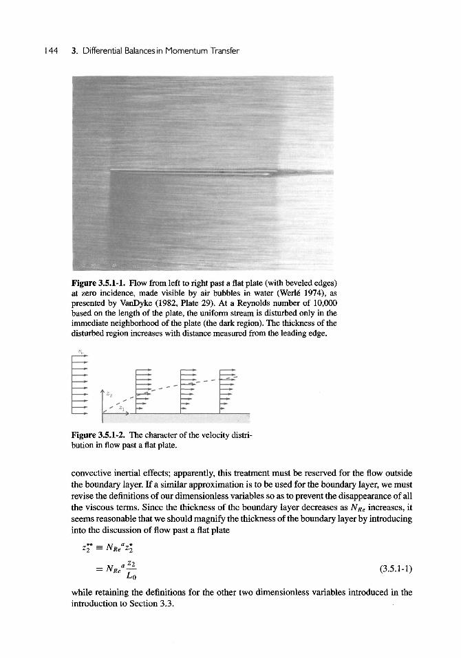
a photograph in which the motion of the particles is not quite stopped (see Figures 3.5.1-1and 3.5.1-3). The traces left by the particles are proportional to the velocity of the fluidat the surface (so long as we assume that very small particles move with the fluid). For asteady-state flow, such a photograph may be used to construct the particle paths. For anunsteady-state flow, it depicts the streamlines, the family of curves to which the velocityvector field is everywhere tangent.
In two-dimensional flows, the streamlines have a special significance. They are curvesalong which the stream function (Sections 1.3.7) is a constant. See Exercise 1.3.7-2.
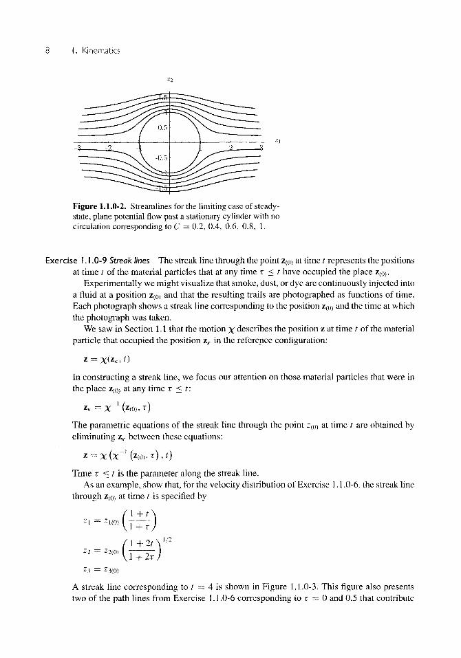
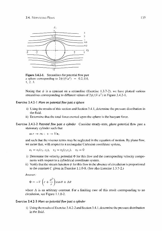
Exercise 1. 1.0-8 For the limiting case of steady-state, plane potential flow past a stationary cylinderof radius a with no circulation, the physical components of velocity in cylindrical coordinatesare (see Exercise 3.4.2-2)
vr = V ( 1 - °- \cos9
ve = -V l + - r sinfl
V ' /and
v2 = 0
Show that the family of streamlines is described by
1 - ~ Jrsin0 =C
Plot representative members of this family as in Figure 1.1.0-2.
I. Kinematics
Figure 1.1.0-2. Streamlines for the limiting case of steady-state, plane potential flow past a stationary cylinder with nocirculation corresponding to C = 0.2, 0.4, 0.6, 0.8, 1.
Exercise 1. 1.0-9 Streak lines The streak line through the point Z(o> at time t represents the positionsat time t of the material particles that at any time r < t have occupied the place Z(o>.
Experimentally we might visualize that smoke, dust, or dye are continuously injected intoa fluid at a position Z(0) and that the resulting trails are photographed as functions of time.Each photograph shows a streak line corresponding to the position z(0) and the time at whichthe photograph was taken.
We saw in Section 1.1 that the motion x describes the position z at time t of the materialparticle that occupied the position zK in the reference configuration:
In constructing a streak line, we focus our attention on those material particles that were inthe place z(0) at any time r < t:
The parametric equations of the streak line through the point z(0) at time t are obtained byeliminating zK between these equations:
' = X (X'1 (z(o>, r ) , t)
Time r < t is the parameter along the streak line.As an example, show that, for the velocity distribution of Exercise 1.1.0-6, the streak line
through Z(0) at time t is specified by
Zl = Z l(O)
2 2 Z 2(O)
1 + T
1+2A'l + 2r J
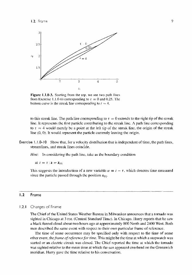
A streak line corresponding to t = 4 is shown in Figure 1.1.0-3. This figure also presentstwo of the path lines from Exercise 1.1.0-6 corresponding to r = 0 and 0.5 that contribute
1.2. Frame
2.5
1.5
T = 0
Figure 1.1.0-3. Starting from the top, we see two path linesfrom Exercise 1.1.0-6) corresponding to r = 0 and 0.25. Thebottom curve is the streak line corresponding to t = 4.
to this streak line. The path line corresponding to r = 0 extends to the right tip of the streakline. It represents the first particle contributing to the streak line. A path line correspondingto R = 4 would merely be a point at the left tip of the streak line, the origin of the streakline (0, 0). It would represent the particle currently leaving the origin.
Exercise 1. 1.0-10 Show that, for a velocity distribution that is independent of time, the path lines,streamlines, and streak lines coincide.
Hint: In considering the path line, take as the boundary condition
at t = X : z = Z(0)
This suggests the introduction of a new variable a = t — r, which denotes time measuredsince the particle passed through the position Z(0).
1.2 Frame
.2.1 Changes of Frame
The Chief of the United States Weather Bureau in Milwaukee announces that a tornado wassighted in Chicago at 3 P.M. (Central Standard Time). In Chicago, Harry reports that he sawa black funnel cloud about two hours ago at approximately 800 North and 2400 West. Bothmen described the same event with respect to their own particular frame of reference.
The time of some occurrence may be specified only with respect to the time of someother event, the frame of reference for time. This might be the time at which a stopwatch wasstarted or an electric circuit was closed. The Chief reported the time at which the tornadowas sighted relative to the mean time at which the sun appeared overhead on the Greenwichmeridian. Harry gave the time relative to his conversation.
I. Kinematics
D (2)
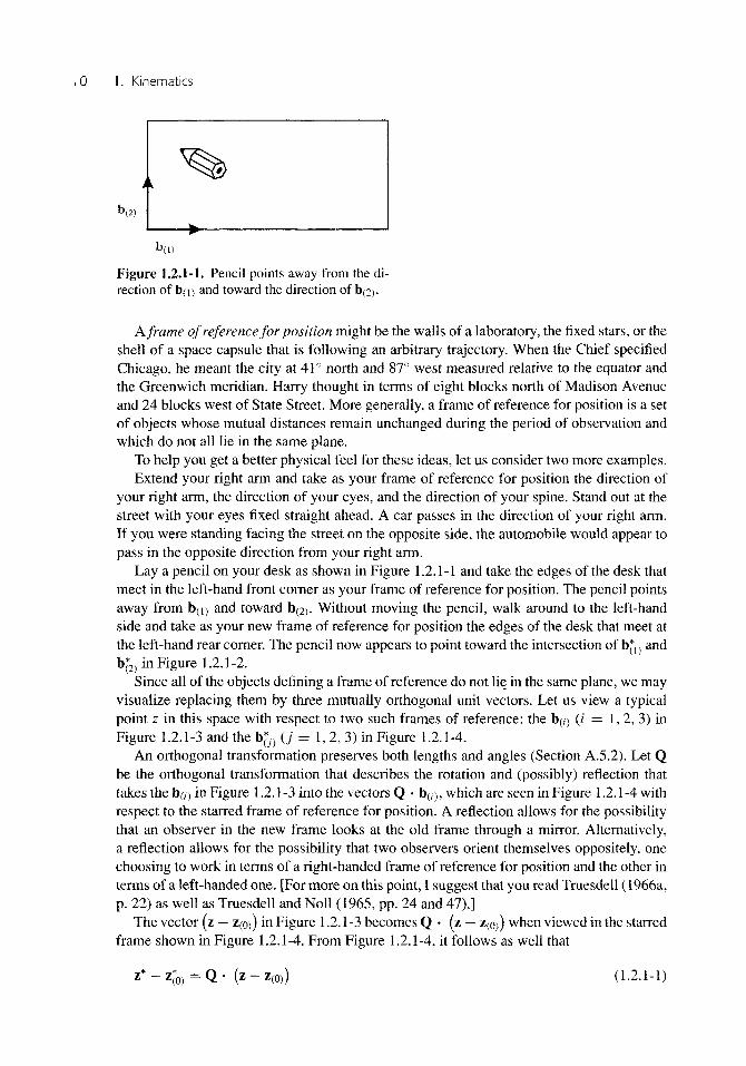
Figure 1.2.1-1. Pencil points away from the di-rection of b(i) and toward the direction of b(2>.
A frame of reference for position might be the walls of a laboratory, the fixed stars, or theshell of a space capsule that is following an arbitrary trajectory. When the Chief specifiedChicago, he meant the city at 41° north and 87° west measured relative to the equator andthe Greenwich meridian. Harry thought in terms of eight blocks north of Madison Avenueand 24 blocks west of State Street. More generally, a frame of reference for position is a setof objects whose mutual distances remain unchanged during the period of observation andwhich do not all lie in the same plane.
To help you get a better physical feel for these ideas, let us consider two more examples.Extend your right arm and take as your frame of reference for position the direction of
your right arm, the direction of your eyes, and the direction of your spine. Stand out at thestreet with your eyes fixed straight ahead. A car passes in the direction of your right arm.If you were standing facing the street on the opposite side, the automobile would appear topass in the opposite direction from your right arm.
Lay a pencil on your desk as shown in Figure 1.2.1-1 and take the edges of the desk thatmeet in the left-hand front corner as your frame of reference for position. The pencil pointsaway from b(i) and toward b(2). Without moving the pencil, walk around to the left-handside and take as your new frame of reference for position the edges of the desk that meet atthe left-hand rear corner. The pencil now appears to point toward the intersection of b*1} andb*2) in Figure 1.2.1-2.
Since all of the objects defining a frame of reference do not lie in the same plane, we mayvisualize replacing them by three mutually orthogonal unit vectors. Let us view a typicalpoint z in this space with respect to two such frames of reference: the b(/) (/ = 1, 2, 3) inFigure 1.2.1-3 and the b*y) 0 = 1, 2, 3) in Figure 1.2.1-4.
An orthogonal transformation preserves both lengths and angles (Section A.5.2). Let Qbe the orthogonal transformation that describes the rotation and (possibly) reflection thattakes the b(/) in Figure 1.2.1-3 into the vectors Q • b(/), which are seen in Figure 1.2.1-4 withrespect to the starred frame of reference for position. A reflection allows for the possibilitythat an observer in the new frame looks at the old frame through a mirror. Alternatively,a reflection allows for the possibility that two observers orient themselves oppositely, onechoosing to work in terms of a right-handed frame of reference for position and the other interms of a left-handed one. [For more on this point, I suggest that you read Truesdell (1966a,p. 22) as well as Truesdell and Noll (1965, pp. 24 and 47).]
The vector (z — z(0)) in Figure 1.2.1-3 becomes Q • (z — Z(0)) when viewed in the starredframe shown in Figure 1.2.1-4. From Figure 1.2.1-4, it follows as well that
z*-z*0 ) = Q . ( z - z ( 0 ) ) (1.2.1-1)
1.2. Frame I i
(1)
Figure 1.2.1-2. Pencil pointstoward the direction 'of b;(and b*2).
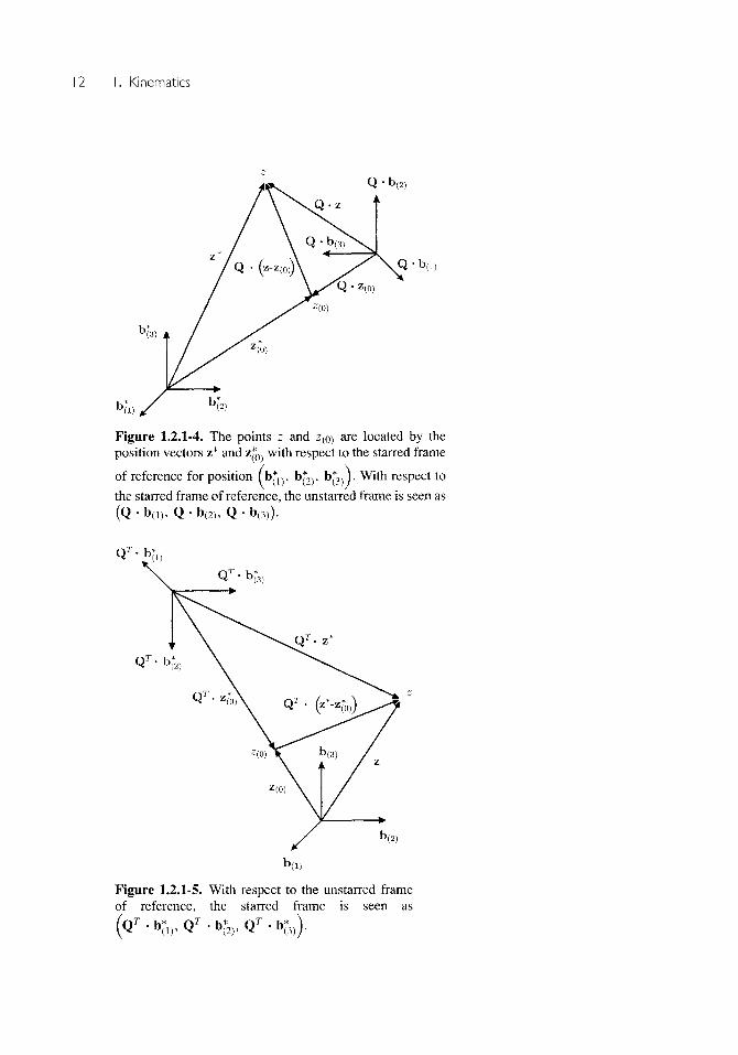
Figure 1.2.1-3. The points z and Z(o> are locatedby the position vectors z and Z(o) with respect to theframe of reference for position (b(i), b(2), b(3)).
Similarly, (z* — z*0)) in Figure 1.2.1-4 is seen as Q r • (z* — z*0)) when observed withrespect to the unstarred frame in Figure 1.2.1-5. Figure 1.2.1-5 also makes it clear that
- Z(0) — Q • (z* - z*0)) (1.2.1-2)
Let z and t denote a position and time in the old frame; z* and t* are the correspondingposition and time in the new frame. We can extend the discussion above to conclude that the
I. Kinematics
Figure 1.2.1-4. The points z and Z(o> are located by theposition vectors z* and z j L with respect to the starred frame
of reference for position (b*1)9 b*2), b*3 ) j . With respect tothe starred frame of reference, the unstarred frame is seen as(Q . b ( i ) , Q • b(2), Q • b (3)).
QT
Q r -b*
Figure 1.2.1-5. With respect to the unstarred frameof reference, the starred frame is seen as
1.2. Frame 13
most general change of frame is of the form
z* =z*0)(0 + Q(0 • (z - z(0)) (1.2.1-3)
t*=t-a (1.2.1-4)
where we allow the two frames discussed in Figures 1.2.1-3 and 1.2.1-4 to rotate and translatewith respect to one another as functions of time. The quantity a is a real number. Equivalently,we could also write
z = ) + Q r • (z* - Z(0)) (1.2.1-5)
t = t*+a (1.2.1-6)
It is important to carefully distinguish between a frame of reference for position and acoordinate system. Any coordinate system whatsoever can be used to locate points in spacewith respect to three vectors defining a frame of reference for position and their intersection,although I recommend that admissible coordinate systems be restricted to those whose axeshave a time-invariant orientation with respect to the frame. Let (z\, z2, z3) be a rectangularCartesian coordinate system associated with the frame of reference (b(1), b(2>, b(3>); simi-larly, let (z*, z|, z|) be a rectangular Cartesian coordinate system associated with anotherframe of reference (b*1); b*2), b*3)). We will say that these two coordinate systems are thesame if the orientation of the basis fields e* with respect to the vectors b(j) is identical to theorientation of the basis fields e* with respect to the vectors b*^:
e/ • b 0 ) = e* • b*;) for all /, j = 1, 2, 3 (1.2.1-7)
We will generally find it convenient to use the same coordinate system in discussing twodifferent frames of reference.
Let us use the same rectangular Cartesian coordinate system to discuss the change offrame illustrated in Figures 1.2.1-4 and 1.2.1-5. The orthogonal tensor
Q = G/ye;ey (1.2.1-8)
describes the rotation (and possibly reflection) that transforms the basis vectors e j (j =1,2,3) into the vectors
Q • e, = g/ye* (1.2.1-9)
which are vectors expressed in terms of the starred frame of reference for position. Therectangular Cartesian components of Q are defined by the angles between the e* and theQ - e , :
Qij = e* • (Q • e,-) (1.2.1-10)
The vector (z — Z((») in Figure 1.2.1-3 becomes
Q • (z - 2(0)) = Qij (zj - z(OW) e(* (1.2.1-11)
when viewed in the starred frame shown in Figure 1.2.1-4. From Figure 1.2.1-4, it followsas well that
* e * = z*0),.e;* + Qu (ZJ - ZMJ) < (1.2.1-12)
14 I. Kinematics
We speak of a quantity as being frame indifferent if it remains unchanged or invariantunder all changes of frame. A frame-indifferent scalar b does not change its value:
b* = b (1.2.1-13)
A frame-indifferent spatial vector remains the same directed line element under a change offrame in the sense that if
u =
then
u*
From
u*
= Z\ -
- z *
(1.2.
= Q
= Q
— Z 2
-z*
1-3),
• (zi
• u
- z 2 )
(1.2.1-14)
A frame-indifferent second-order tensor is one that transforms frame-indifferent spatialvectors into frame-indifferent spatial vectors. If
u = Tw (1.2.1-15)
the requirement that T be a frame-indifferent second-order tensor is
u* = T*•w* (1.2.1-16)
where
u* = Q • u(1.2.1-17)
w* = Q • w
This means that
Q • u = T* • Q • w
= Q T w (1.2.1-18)
which implies
T = Q r - T * Q (1.2.1-19)
or
T * = Q . T - Q r (1.2.1-20)
The importance of changes of frame will become apparent in Section 2.3.1, where theprinciple of frame indifference is introduced. This principle will be used repeatedly indiscussing representations for material behavior and in preparing empirical data correlations.
The material in this section is drawn from Truesdell and Toupin (1960, p. 437), Truesdelland Noll (1965, p. 41), and Truesdell (1966a, p. 22).
1.2. Frame 15
Exercise 1.2.1-1 Let T be a frame-indifferent scalar field. Starting with the definition of thegradient of a scalar field in Section A.3.1, show that the gradient of T is frame indifferent:
vr* = (vry = Q • vr
Exercise I.2.1 -2 In order that e (defined in Exercise A.7.2-11) be a frame-indifferent third-ordertensor field, prove that
e* = (
1.2.2 Equivalent Motions
In Section 1.1,1 described the motion of a material with respect to some frame of referenceby
z = X ( W ) (1.2.2-1)
where we understand that the form of this relation depends upon the choice of referenceconfiguration K. According to our discussion in Section 1.2.1, the same motion with respectto some new frame of reference is represented by
[Xtot, 0 - *>] (1.2.2-2)
We will say that any two motions x a n d X* related by an equation of the form of (1.2.2-2)are equivalent motions.
Let us write (1.2.2-2) in an abbreviated form:
z * = z ; + Q . ( z - z 0 ) (1.2.2-3)
The material derivative of this equation gives
v* = — + — • ( z - z 0 ) + Q • v (1.2.2-4)at at
or
v * - Q • v = — + — • ( z - z o ) (1.2.2-5)
In view of (1.2.2-3), we may writez - z0 = Q r • Q • (z - z0)
= Q r - ( z * - z £ ) (1.2.2-6)
This allows us to express (1.2.2-5) as
dz*0V-Q-v =
(1.2.2-7)
16 I. Kinematics
where
A=—QT (1.2.2-8)dt
We refer to the second-order tensor A as the angular velocity tensor of the starred framewith respect to the unstarred frame (Truesdell 1966a, p. 24).
Since Q is an orthogonal tensor,
Q Q r = T (1.2.2-9)
Taking the material derivative of this equation, we have
\dt)
(1.2.2-10)
In this way we see that the angular velocity tensor is skew symmetric.The angular velocity vector of the unstarred frame with respect to the starred frame u? is
defined as
UJ=- t r ( e* -A) (1.2.2-11)
The third-order tensor e is introduced in Exercises A.7.2-11 and A.7.2-12 (see also Exercise1.2.1-2), where tr denotes the trace operation defined in Section A.7.3. Let us consider thefollowing spatial vector in rectangular Cartesian coordinates:
u,A (z*-O=tr(e*. [(z* - zj) u,])
= tr(e*. {[z*-z*]jjtr(e*.A)]j)
- (z*k - z*Ok) Aike*
= A - (z* - z*) (1.2.2-12)
We may consequently write (1.2.2-7) in terms of the angular velocity of the unstarred framewith respect to the starred frame (Truesdell and Toupin 1960, p. 437):
v* = ^ + w A[Q.(z-zdz*dto)] + Q . v (1.2.2-13)
1.2. Frame 17
The material in this section is drawn from Truesdell and Noll (1965, p. 42) and Truesdell(1966a, p. 22).
Exercise 1.2.2-1
i) Show that velocity is not frame indifferent.ii) Show that at any position in euclidean point space a difference in velocities with respect
to the same frame is frame indifferent.
Exercise 1.2.2-2 Acceleration
i) Determine that (Truesdell 1966a, p. 24)
4m)V* = fK , 2 A . (y*_d^dt dt2 ' I dt
ii) Prove that (Truesdell and Toupin 1960, p. 440)
iii) Prove that
u> A [u> A (z* - z*)] = A • A • (z* - z*)
^ A A(z*-z* ) = ^ . ( z * - z * )
and
CJ A (Q • v) = A • Q • v
iv) Conclude that (Truesdell and Toupin 1960, p. 438)
A w A [Q . (z - z0)]}
u, A .(Q.VV)) + Q%V)) + Q %dt
Exercise 1.2.2-3 Give an example of a scalar that is not frame indifferent.
Hint: What vector is not frame indifferent?
18 I. Kinematics
Exercise 1.2.2-4 Motion of a rigid body Determine that the velocity distribution in a rigid body maybe expressed as
What is the relation of the unstarred frame to the body in this case?
1.3 Mass
1.3.1 Conservation of Mass
This discussion of mechanics is based upon several postulates. The first is
Conservation of mass The mass of a body is independent of time.
Physically, this means that, if we follow a portion of a material body through any numberof translations, rotations, and deformations, the mass associated with it will not vary as afunction of time. If p is the mass density of the body, the mass may be represented as
fJRu
Here dV denotes that a volume integration is to be performed over the region i?(m) of spaceoccupied by the body in its current configuration; in general R(m), or the limits on thisintegration, is a function of time. The postulate of conservation of mass says that
pdV=0 (1.3.1-1)
Notice that, like the material particle introduced in Section 1.1, mass is a primitive concept.Rather than defining mass, we describe its properties. We have just examined its mostimportant property: It is conserved. In addition, I will require that
p>0 (1.3.1-2)
and that the mass density be a frame-indifferent scalar,
p* = p (1.3.1-3)
Our next objective will be to determine a relationship that expresses the idea of conserva-tion of mass at each point in a material. To do this, we will find it necessary to interchangethe operations of differentiation and integration in (1.3.1-1). Yet the limits on this integraldescribe the boundaries of the body in its current configuration and generally are functionsof time. The next section explores this problem in more detail.
1.3.2 Transport Theorem
Let us consider the operation
d
It•I
1.3. Mass 19
Here *I> is any scalar-, vector-, or tensor-valued function of time and position. Again, weshould expect R(m), or the limits on this integration, to be a function of time.
If we look at this volume integration in the reference configuration K, the limits onthe volume integral are no longer functions of time; the limits are expressed in terms ofthe material coordinates of the bounding surface of the body. This means that we mayinterchange differentiation and integration in the above operation. In terms of a rectangularCartesian coordinate system, let (z\,zi, Z3) denote the current coordinates of a material pointand let (zK\, zK2, zKz) be the corresponding material coordinates. Using the results of SectionA. I1.3, we may say that
= — / VJdV
) R { m ) K \ dt j dt J
__ I I (m) (m)
j R \ dt J dt(1.3.2-1)
where (see Exercise A. I1.3-1)
dzij = det
= det
= |detF| (1.3.2-2)
Here
F =
azj (
dzKJ(1.3.2-3)
is the deformation gradient. The quantity / may be thought of as the volume in the currentconfiguration per unit volume in the reference configuration. It will generally be a functionof both time and position. Here R(m)K indicates that the integration is to be performed overthe region of space occupied by the body in its reference configuration K.
What follows is the most satisfying development of (1.3.2-8). If this is your first timethrough this material, I recommend that you replace (1.3.2-3) through (1.3.2-7) by thealternative development of (1.3.2-8) in Appendix B.
From Exercise A. 10.1-5,
d(m)J
dt \ dt
It is easy to show that
F~' =dz
~dzZemen
(1.3.2-4)
(1.3.2-5)
20 I. Kinematics
Using the definition of velocity from Section 1.1, we have
d(m)¥ dvi dvt dzr
Consequently,
_ d zKJ dvt dzr
dt ) dzi dzr dzKj
dzt
divv (1.3.2-7)
and
1 d(m)J= divv
/ dt
Equation (1.3.2-8) allows us to write (1.3.2-1) as
-/x VdV=f f ^ + x I / d i v v W dV(1.3.2-9)dt JR{m) JRm) V dt )
This may also be expressed as
— / VdV= —+div(^\)\dV (1.3.2-10)dt— J/R(m) VdV=J—+R(m) I dt J
or, by Green's transformation (Section A.1 1.2), we may say
— / VdV^f — d V + f Vv-ndA (1.3.2-11)dt JR{m) JR(m} dt JS(m)
By S(m), I mean the closed bounding surface of R(my, like R(m), it will in general be a functionof time. Equations (1.3.2-9) to (1.3.2-11) are three forms of the transport theorem (Truesdelland Toupin l960, p. 347).
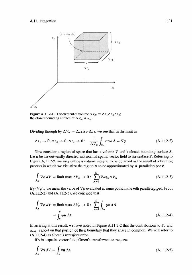
We will have occasion to ask about the derivative with respect to time of a quantity whilefollowing a system that is not necessarily a material body. For example, let us take as oursystem the air in a child's balloon and ask for the derivative with respect to time of the volumeassociated with the air as the balloon is inflated. Since material (air) is being continuouslyadded to the balloon, we are not following a set of material particles as a function of time.However, there is nothing to prevent us from defining a particular set of fictitious systemparticles to be associated with our system. The only restriction we shall make upon thisset of imaginary system particles is that the normal component of velocity of any systemparticle at the boundary of the system be equal to the normal component of velocity of theboundary of the system. Equations (1.3.2-8) to (1.3.2-11) remain valid if we replace
1) derivatives with respect to time while following material particles, d(m)/dt, by derivativeswith respect to time while following fictitious system particles, d(S)/dt; and
2) the velocity vector for a material particle, v, by the velocity vector for a fictitious systemparticle, v(s).
1.3. Mass 21
This means that
— / tydV= — d V + / *v ( j )-na!A (1.3.2-12)dt J^ JR{S) dt JSis)
Here R(S) signifies that region of space currently occupied by the system; S(S) is the closedbounding surface of the system. We will refer to (1.3.2-12) as the generalized transporttheorem (Truesdell and Toupin 1960, p. 347).
For an alternative discussion of the transport theorem, see Appendix B.
Exercise 1.3.2-1 Show that
— f dV = I divvdV = I Y-ndA"t jR{m) jR(mj Js{m)
Here S(m) is the (time-dependent) closed bounding surface of R(m).
1.3.3 Differential Mass Balance
Going back to the postulate of conservation of mass in Section 1.3.1,1 n
— / pdV = 0 (1.3.3-1)dt jR<m)
and employing the transport theorem in the form of (1.3.2-9), we have that
{ m ) p p d i v v r f V = 0 (1.3.3-2)dt )
But this statement is true for any body or for any portion of a body, since a portion of a bodyis a body (see Exercise 1.3.3-4). We conclude that the integrand itself must be identicallyzero:
/odivv = 0 (1.3.3-3)+pdivv 0dt
By Exercise 1.1.0-1, this may also be written as
— +div(pv) = 0 (1.3.3-4)at
Equations (1.3.3-3) and (1.3.3-4) are two forms of the equation of continuity or differentialmass balance. These equations express the requirement that mass be conserved at everypoint in the continuous material.
The differential mass balance is presented in Table 2.4.1-1 for rectangular Cartesian,cylindrical, and spherical coordinates.
If the density following a fluid particle does not change as a function of time, (1.3.3-3)reduces to
divv = 0 (1.3.3-5)
Such a motion is said to be isochoric. If, for the flow under consideration, density is inde-pendent of both time and position, we will say that the fluid is incompressible. A sufficient,though not necessary, condition for an isochoric motion is that the fluid is incompressible.
22 I. Kinematics
Exercise 1.3.3-1 Another form of the transport theorem Show that, i f we assume that mass isconserved, for any $
Exercise 1.3.3-2 Derive the forms of the differential mass balance shown in Table 2.4.1 -1.
Exercise 1.3.3-3
i) From (1.3.2-1) and the postulate of conservation of mass, determine that
ii) Integrate this equation to conclude that
/ = |detF|_ A)
P
where p0 denotes the density distribution in the reference configuration.
Exercise 1.3.3-4 When volume integral over arbitrary body is zero, the integrand is zero. Let us examinethe argument that must be supplied in going from (1.3.3-2) to (1.3.3-3).
We can begin by considering the analogous problem in one dimension. It is clear that
f2
/
Jo/
Jo
does not imply that sin 0 is identically zero. But
f f(y)dy = 0 (1.3.3-6)Jo
does imply that
/O0 = 0 (1.3.3-7)
Proof: The Leibnitz rule for the derivative of an integral states that (Kaplan 1952, p. 220)
Equation (1.3.3-7) follows immediately.Let us consider the analogous problem for
/ dg(x) dx
PKI rm(z) /-feCv.z)
/ / / g(x,y,z)dxdydz = 0 (1.3.3-8)
1.3. Mass 23
where £i(j,z), %2(y, z), rji(z), ti2(z), fi, and & a r e completely arbitrary. Prove that thisimplies
g(x,y,z) = 0 (1.3.3-9)
Exercise 1.3.3-5 Frame indifference of differential mass balance Prove that the differential massbalance takes the same form in every frame of reference.
1.3.4 Phase Interface
A phase interface is that region separating two phases in which the properties or behaviorof the material differ from those of the adjoining phases. There is considerable evidencethat density is appreciably different in the neighborhood of an interface (Defay et al. 1966,p. 29). As the critical point is approached, density is observed to be a continuous functionof position in the direction normal to the interface (Hein 1914; Winkler and Maass 1933;Maass 1938; Mclntosh et al. 1939; Palmer 1952). This suggests that the phase interfacemight be best regarded as a three-dimensional region, the thickness of which may be severalmolecular diameters or more.
Although it is appealing to regard the interface as a three-dimensional region, there isan inherent difficulty. Except in the neighborhood of the critical point where the interfaceis sufficiently thick for instrumentation to be inserted, the density and velocity distributionsin the interfacial region can be observed only indirectly through their influence upon theadjacent phases.
Gibbs (1928, p. 219) proposed that a phase interface at rest or at equilibrium be regardedas a hypothetical two-dimensional dividing surface that lies within or near the interfacialregion and separates two homogeneous phases. He suggested that the cumulative effects ofthe interface upon the adjoining phases be taken into account by the assignment to the dividingsurface of any excess mass or energy not accounted for by the adjoining homogeneous phases.
Gibbs's concept may be extended to include dynamic phenomena if we define a homo-geneous phase to be one throughout which each description of material behavior appliesuniformly. In what follows, we will represent phase interfaces as dividing surfaces. In mostproblems of engineering significance, we can neglect the effects of excess mass, momen-tum, energy, and entropy associated with this dividing surface. For this reason, they will beneglected here. For a more detailed discussion of these interfacial effects, see Slattery (1990).
1.3.5 Transport Theorem for a Region Containing a Dividing Surface
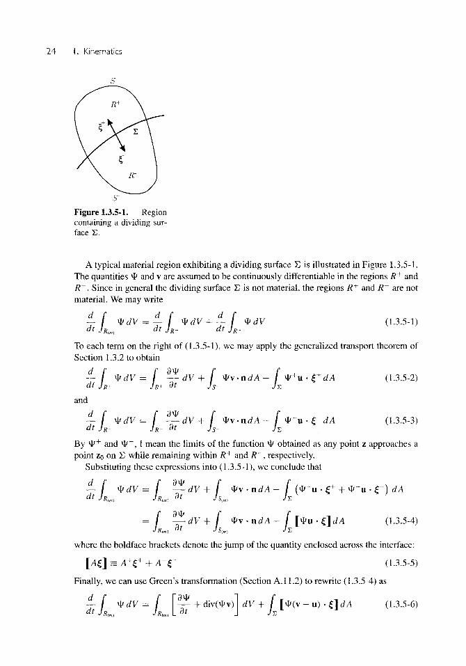
As described in the preceding section, we will be representing the phase interface as adividing surface, a surface at which one or more quantities such as density and velocity arediscontinuous. In general, a dividing surface is not material; it is common for mass to betransferred across it. As an ice cube melts, as water evaporates, or as solid carbon dioxidesublimes, material is transferred across it and the phase interface moves through the material.We assume that this dividing surface may be in motion through the material with an arbitraryspeed of displacement. If u denotes the velocity of a point on the surface, u • £+ is the speedof displacement of the surface measured in the direction £ + in Figure 1.3.5-1, and u • £~ isthe speed of displacement of the surface measured in the direction £~ (Truesdell and Toupin1960, p. 499).
24 I. Kinematics
Figure 1.3.5-1. Regioncontaining a dividing sur-face S.
A typical material region exhibiting a dividing surface E is illustrated in Figure 1.3.5-1.The quantities *V and v are assumed to be continuously differentiate in the regions R+ andR~. Since in general the dividing surface £ is not material, the regions R+ and R~ are notmaterial. We may write
— f Vd [ —l VdV + f VdV (1.3.5-1)dt JR(m) dt JR+ dt JR-
To each term on the right of (1.3.5-1), we may apply the generalized transport theorem ofSection 1.3.2 to obtain
d_
dt
and
d
f VdV = f -dV + / VvndA - / V+u * £+dA (1.3.5-2)JR+ JR+ dt Js+ ]•£,
fJR-dt JR- JR- dt Js- JE
By * + and *I>~", I mean the limits of the function ty obtained as any point z approaches apoint z0 on E while remaining within R+ and R~, respectively.
Substituting these expressions into (1.3.5-1), we conclude thatd f f 9* f f ( + +
di JR{m) " dt JR(m) A= 1 — dV + 1 * v - n d A - / [*u*£\dA (1.3.5-4)
where the boldface brackets denote the jump of the quantity enclosed across the interface:
[A{] = A Y + A T (1.3.5-5)
Finally, we can use Green's transformation (Section A.I 1.2) to rewrite (1.3.5-4) as
Iv / VdV= ( — h * d i v v | d V + / F * ( v - u ) -£\dA (1.3.5-7)jR,m, JR{m \ dt J JX
We will refer to (1.3.5-7) as the transport theorem for a region containing a dividing surface.This discussion is based upon that of Truesdell and Toupin (1960, p. 525).
1.3.6 Jump Mass Balance for Phase Interface
In Section 1.3.3, we found that the differential mass balance expresses the requirement thatmass is conserved at every point within a continuous material. We wish to examine theimplications of mass conservation at a phase interface. As described in Section 1.3.4, wewill represent the phase interface as a dividing surface, rather than as a three-dimensionalregion of some thickness.
Equation (1.3.1-1) again applies to the multiphase body drawn in Figure 1.3.5-1;
— / pdV = 0 (1.3.6-1)
By the transport theorem for a region containing a dividing surface given in Section 1.3.5,Equation (1.3.6-1) may be written as
—f pdV=f (d^-+p&\v\\dV + f [p(v-u)•£]dA (1.3.6-2)dt JKm) JRm V dt ) hSince the differential mass balance developed in Section 1.3.3 applies everywhere within
each phase, (1.3.6-2) reduces to
/ [ p ( v - u ) -C]dA = 0 (1.3.6-3)
This must be true for any portion of a body containing a phase interface, no matter how largeor small the body is. We conclude that the integrand itself must be zero:
f r ( v - u ) - € ] = 0 (1.3.6-4)
This is known as the jump mass balance for a phase interface, which is represented by adividing surface, when all interfacial effects are neglected (Slattery 1990).
Exercise 1.3.6-1 Discuss how one concludes that, when there is no mass transfer across the phaseinterface, (1.3.6-4) reduces to
u • £ = v+ • £ = v" • £
Exercise 1.3.6-2 Alternative derivation of jump mass balance Write the postulate of conservationof mass for a material region that instantaneously contains a phase interface. Employ thetransport theorem for a region containing a dividing surface in the form of (1.3.5-4). Deducethe jump mass balance (1.3.6-4) by allowing the material region to shrink around the phaseinterface (surface of discontinuity) (Truesdell and Toupin 1960, p. 526).
26 I. Kinematics
Exercise 1.3.6-3 Alternative form of transport theorem for regions containing a dividing surface Showthat, since mass is conserved, for any 4*
^f p4*dV =f^f p4*dV=f p^dVdtJR{m) JRm dt
Exercise 1.3.6-4 Frame indifference of jump mass balance Prove that the jump mass balance takesthe same form in every frame of reference.
1.3.7 Stream Functions
By a two-dimensional motion, we mean here one such that in some coordinate system thevelocity field has only two nonzero components.
Let us further restrict our discussion to incompressible fluids, so that the differential massbalance (1.3.3-3) reduces to
divv = 0 (1.3.7-1)
Consider a two-dimensional motion such that in spherical coordinates
vr = iv(r, 9), v0 = ve(r, 9), vv = 0 (1.3.7-2)
From Table 2.4.1-1, Equation (1.3.7-1) takes the form
1 9 , 1 3- — (r2vr) + : ( v e sin#) = 0 (1.3.7-3)r2 dr r sm# 80
Multiplying by r2 sin 9, we may also write this as
d , 9— (vrr
2sin9) = — {-v0r sin£) (1.3.7-4)9r 3#
Upon comparing (1.3.7-4) with
d7d9 = Wd~r~ ( L 1 7 " 5 )
we see that we may define a stream function \jr such that
»- = —— S (1.3.7-6)
and
^ ^ p (1.3.7-7)r
The advantage of such a stream function i/r is that it can be used in this way to satisfyidentically the differential mass balance for the flow described by (1.3.7-2).
Expressions for velocity components in terms of a stream function are presented forseveral situations in Tables 2.4.2-1.
Exercise 1.3.7-1 Using arguments similar to those employed in this section, for each velocitydistribution in Table 2.4.2-1, express the nonzero components of velocity in terms of astream function.
1.3. Mass 27
Exercise 1.3.7-2 Stream function is a constant along a streamline. Prove that, in a two-dimensionalflow, the stream function is a constant along a streamline. This allows one to readily plotstreamlines as in Figures 1.1.0-2 and 3.4.2-1.
Hint: Let a be a parameter measured along a streamline. Begin by recognizing that
dp— A v = 0.da
Exercise 1.3.7-3 Another view of the stream function Show that the differential mass balance for anincompressible fluid in a two-dimensional flow can be expressed as
9 , _ c
dx' ' dx2'
This is a necessary and sufficient condition for the existence of a stream function i/r suchthat
For further discussion of these ideas as well as an extension of the concept of a streamfunction to steady compressible flows, see Truesdell and Toupin (1960, p. 477).
2
Foundations for Momentum Transfer
I N WHAT FOLLOWS, the principal tools for studying fluid mechanics are developed.We begin by introducing the concept of force. Notice that force is not defined; it is a
primitive concept in the same sense as is mass and the material particle in Chapter 1. Thisforms the basis for introducing our second and third postulates: the momentum balance andthe moment of momentum balance. The stress tensor is introduced in order to derive theequations that describe at each point in a material the local balances for momentum andmoment of momentum. The differential mass and momentum balances together with thesymmetry of the stress tensor form the foundation for fluid mechanics.
We conclude our discussion with an outline of what must be said about real materialbehavior if we are to analyze any practical problems. It is especially at this point thatstatistical mechanics, based upon the molecular viewpoint of real materials, can be used tosupplement the concepts developed in continuum mechanics. In continuum mechanics, wecan indicate a number of rules that constitutive equations for the stress tensor must satisfy(the principle of determinism, the principle of local action, the principle of material frameindifference,...), but from first principles we cannot derive an explicit relationship betweenstress and deformation. If we work strictly within the bounds of continuum mechanics, wecan derive such a relationship only by making some sort of assumption about its form. Ourfeelings are that the most interesting advances in describing material behavior result frompredictions based upon simple molecular models that are generalized through the use of thestatements about material behavior that have been postulated in continuum mechanics. Foran excellent brief summary of what can be said about material behavior from a molecularpoint of view, see Bird et al. (1960, Chap. 1).
Although our direct concerns here are for momentum transfer, practically all of the ideasdeveloped will be applied again in examining energy and mass transfer. We firmly believethat the best foundation for energy and mass-transfer studies is a clear understanding of fluidmechanics.
2.1 Force
Like the material particle, force is a primitive concept. It is not defined. Instead we des-cribe its attributes in a series of five axioms.
2.1. Force 29
Corresponding to each body B, there is a distinct set of bodies Be such that the mass ofthe union of these bodies is the mass of the universe. We refer to Be as the exterior or thesurroundings of the body B.
a) A system of forces is a vector-valued function f(B, C) of pairs of bodies. The value off(#, C) is called the force exerted on the body B by the body C.
b) For a specified body B, f(C, Be) is an additive function defined over the subbodiesC of B.c) Conversely, for a specified body B, f(#, C) is an additive function defined over the sub-
bodies C of Be.d) In any particular problem, we regard the forces exerted upon a body as being given a priori
to all observers; all observers would assume the same set of forces in a given problem.In prescribing these forces, we specify a particular dynamic problem. We consequentlyassume that all forces are independent of the observer or are frame indifferent (Truesdell1966a, p. 27) (see Section 1.2.1):
f* = Q . f (2.1.0-1)
There are three types of forces with which we may be concerned:
External forces These arise at least in part from outside the body and act upon the material particlesof which the body is composed. One example is the uniform force of gravity. Another examplewould be the electrostatic force between two charged bodies. Let P indicate a portion of abody B as illustrated in Figure 2.1.0-1. Taking fe to be external force per unit mass that thesurroundings Be exert on the body B, we write the total external force acting on P in termsof a volume integral over the region occupied by P:
ffRP
In general, the external force per unit mass is a function of position, and fe should be regardedas a spatial vector field.
Mutual forces These arise within a body and act upon pairs of material particles. The long-rangeintermolecular forces acting between a thin film of liquid and the solid upon which it restsare mutual forces. We can imagine a body in which there is a distribution of electrostaticcharge; we would speak of the electrostatic force between one portion of the body with a netpositive charge and some other element of the body with a net negative charge as being a
Figure 2.1.0-1. The body B of which P is aportion.
30 2. Foundations for Momentum Transfer
mutual force. Let fm be the mutual force per unit mass that B — Pl exerts upon P; the totalmutual force acting upon P may be represented as an integral over the volume of P?
f pfmdVJRP
We should expect the mutual force per unit mass generally to be a function of position withinthe material; fm should be viewed as a spatial vector field.
Contact forces These forces are not assignable as functions of position but are to be imagined asacting upon the bounding surface of a portion of material in such a way as to be equivalentto the force exerted by one portion of the material upon another beyond that accounted forthrough mutual forces. In typing you exert a contact force upon the keys of the typewriter. Ifwe deform some putty in our hands, during the deformation any one portion of the putty exertsa contact force upon the remainder at their common boundary. Let t = t(z, P) represent thestress vector or force per unit area that B — P exerts upon the boundary of P at the positionz. This force per unit area t is usually referred to as stress. The total contact force that B — Pexerts upon P may be written as an integral over the bounding surface of P:
fJSp
tdA
The fifth axiom, the stress principle, specifies the nature of the contact load.
e) Stress principle There is a vector-valued function t(z, n) defined for all points z in abody B and for all unit vectors n such that the stress that B — P exerts upon any portionP of B is given by
t(z, P) = t(z, n) (2.1.0-2)
Here n is the unit normal that is outwardly directed with respect to the closed boundingsurface of P. The spatial vector t = t(z, n) is referred to as the stress vector at the positionz acting upon the oriented surface element with normal n; n points into the material thatexerts the stress t upon the surface element.
The material in this section is drawn from Truesdell (1966b, p. 97), Truesdell and Toupin(1960, pp. 531 and 536) and Truesdell and Noll (1965, p. 39).
2.2 Additional Postulates
2.2.1 Momentum and Moment of Momentum Balance
In Section 1.3.1, we introduced our first postulate, conservation of mass. Our second postulateis (Truesdell 1966b, p. 97; Truesdell and Toupin 1960, pp. 531 and 537; Truesdell and Noll1965, p. 39)3
1 We define B - P to be such that B = (B - P) U P and (B - P) n P = 0.2 We recognize here that the sum of the mutual forces exerted by any two parts of P upon each other is
zero (Truesdell and Toupin 1960, p. 533).3 Truesdell and Toupin (1960, pp. 531 and 534) point out that "the laws of Newton . . . are neither
unequivocally stated nor sufficiently general to serve as a foundation for continuum mechanics."
2.2. Additional Postulates 3 I
Momentum balance The time rate of change of the momentum of a body relative to an inertialframe of reference is equal to the sum of the forces acting on the body.
Let the volume and closed bounding surface of a body or any portion of a body be denoted,respectively, as Rim) and S(m). Referring to our discussion of forces in the introduction toSection 2.1, in an inertial frame of reference we may express the momentum balance as
dIt
f p\dV = f tdA+ f pfdV (2.2.1-1)
Here f is the field of external and mutual forces per unit mass:
f=f,+fw (2.2.1-2)
In most cases, the effect of mutual forces can be neglected with respect to external forces,one of the primary exceptions being thin films, where long-range, intermolecular forcesexerted by the adjoining phases must be taken into account. Hereafter we will assume thatmutual forces have been dismissed, and we will refer to f as the field of external forces perunit mass.
Our understanding is that (2.2.1-1) is written with respect to an inertial frame of reference.In reality, we define an inertial frame of reference to be one in which (2.2.1-1) and (2.2.1-3)are valid. Somewhat more casually we describe an inertial frame of reference to be one thatis stationary with respect to the fixed stars.
Our third postulate is (Truesdell 1966b, p. 97; Truesdell and Toupin 1960, pp. 531 and537; Truesdell and Noll 1965, p. 39).
Moment of momentum balance The time rate of change of the moment of momentum of a bodyrelative to an inertial frame of reference is equal to the sum of the moments of all the forcesacting on the body.
In an inertial frame of reference, the moment of momentum balance assumes the form
— / p(pA\)dV = I pAtdA+ f p(pAf)dV (2.2.1-3)
In writing the moment of momentum balance in this manner we confine our attention tothe so-called nonpolar4 case [i.e., we assume that all torques acting on the body are theresult of forces acting on the body (Truesdell and Toupin 1960, pp. 538 and 546; Curtiss1956; Livingston and Curtiss 1959; Dahler and Scriven 1961)]. For example, it is possibleto induce a local source of moment of momentum by use of a suitable rotating electric field(Lertes 1921a,b,c; Grossetti 1958,1959). In such a case it might also be necessary to accountfor the flux of moment of momentum at the bounding surface of the body. Effects of thistype have not been investigated thoroughly, but they are thought to be negligibly small forall but unusual situations. Consequently, they are neglected here.
4 When molecules are referred to as nonpolar, it indicates that their dipole moment is zero. This is anentirely different use of the word than that intended here, where nonpolar means that all torques actingon the material are the result of forces.
32 2. Foundations for Momentum Transfer
Figure 2.2.2-1. A material body in the form of a tetrahe-dron.
Exercise 2.2.1 -1 Cauchy's lemma Consider two neighboring portions of a continuous body. Applythe momentum balance to each portion and to their union. Deduce that on their commonboundary
t(z, n) = -t(z, - n )
or
Cauchy's lemma The stress vectors acting upon opposite sides of the same surface at a given pointare equal in magnitude and opposite in direction.
2.2.2 Stress Tensor
We ask here how t(z, n) varies as the position z is held fixed and n changes.At any point in a body, consider the tetrahedron shown in Figure 2.2.2-1. Three sides
are mutually orthogonal and coincide with a set of rectangular Cartesian coordinate planesintersecting at z; the fourth side has an outwardly directed normal n. Let the altitude of thetetrahedron be h; let the area of the inclined face be A. In terms of the rectangular Cartesianbasis fields, we may write n = «,e,.
Let us apply the momentum balance (2.2.1-1) to the material in the tetrahedron at time tto obtain
(2.2.2-1)— f pvdV = f tdA+ f pfdV
Applying the form of the transport theorem introduced in Exercise 1.3.3-1 to the term onthe left and using the theorem of mean value to evaluate the surface integral, we have
L( d(m)\dV=Alt* + — (2.2.2-2)
2.2. Additional Postulates 33
Here the asterisk denotes a mean value of the function, t* denotes the contact stress thatthe surroundings exert upon the inclined face, and t* denotes the contact stress that thesurroundings exert upon the face whose inwardly directed unit normal is e?. Applying thetheorem of mean value to the term on the left, we write
^ = A(t* + «1tt + «2^ + n3t*) (2.2.2-3)
Since the cosines of the angles between the Cartesian coordinate planes and the inclinedplane are «i, ri2, and «3, respectively, the areas of the faces of the tetrahedron lying in thecoordinate planes are n\A, /22A, and «3A. Consider a sequence of geometrically similartetrahedrons; in the limit as h approaches zero, we obtain
t = - ( t n i + t / ! 2 + t * 3 ) (2.2.2-4)
where all stress vectors are evaluated at the point z. From their definitions, the quantitiesti, t2, and t3 do not depend upon n.
With the convention that 7im is the kth component of the stress vector acting upon thepositivt side of the plane zm = constant (such that the unit normal is em), by Cauchy's lemma(Exercise 2.2.1-1) we write
- t i = T e i
- t = 7-e / (2.2.2-5)
- t =
This permits us to express (2.2.2-4) as
t = njTijei (2.2.2-6)
The matrix [7}y] defines a second-order stress tensor T:
T = Tije&j (22.2-1)
and (2.2.2-6) becomes
t = T • n (2.2.2-8)
Remember in using (2.2.2-8) that n is the unit normal directed into the material that isexerting the force per unit area t(z, n) at the position z on the surface.
Exercise 2.2.2-1 Show that the stress tensor is frame indifferent.
Exercise 2.2.2-2 In going from (2.2.2-2) to (2.2.2-3), prove that
m = ^-, i = 1,2,3A
2.2.3 Differential and Jump Momentum Balances
A modification of the transport theorem that takes into account the postulate that mass isconserved (see Exercise 1.3.6-3) may be used to express the momentum balance (2.2.1-1)as
p^-dV + f [pv(v - u) • (\dA = f tdA+ f pfdV (2.2.3-1)dt JE JS(m) JR{m)
34 2. Foundations for Momentum Transfer
If we express the stress vector t in terms of the stress tensor T as suggested in Section 2.2.2,the first term on the right of this equation may be rearranged by an application of Green'stransformation (Section A.I 1.2):
f tdA = f T •ndA'sim} Jslm)
= ff divlW + / [T•£]dA (2.2.3-2)
Substituting (2.2.3-2) into (2.2.3-1), we have
dV + [ [pv(v-u) '£-T.£\dA = 0 (2.2.3-3)fRemember that (2.2.3-1) is written for an arbitrary portion P of a body. Whether P isvery large or arbitrarily small or whether P consists of one phase or many phases,(2.2.3-3) remains valid. This implies that the differential momentum balance (Cauchy' s first"law"),
(2.2.3-4)pdt
must be satisfied at each point within each phase and that the jump momentum balance,
[pv(v-u) - £ - T . £ ] = 0 (2.2.3-5)
must be obeyed at each point on each phase interface. Here u • £ is the speed of displacementof the phase interface; the boldface bracket notation is defined in Section 1.3.5.
Exercise 2.2.3-1 Archimedes principles Prove the following two theorems of Archimedes (Rouseandlnce l957, p. 17):
If a solid lighter than a fluid be forcibly immersed in it, the solid will be driven upwardsby a force equal to the difference between its weight and the weight of the fluid displaced.
A solid heavier than a fluid will, if placed in it, descend to the bottom of the fluid, andthe solid will, when weighed in the fluid, be lighter than its true weight by the weight ofthe fluid displaced.
Hint: Apply the momentum balance and extend the definition of fluid pressure into theregion of space occupied by the solid, recognizing that pressure in the fluid is a constant inany horizontal plane.
Exercise 2.2.3-2 Another theorem of Archimedes Prove (Rouse and Ince 1957, p. 17):
Any solid lighter than a fluid will, if placed in the fluid, be so far immersed that theweight of the solid will be equal to the weight of the fluid displaced.
Hint: Proceed as in Exercise 2.2.3-1, making use of the jump momentum balance(2.2.3-5).
2.2. Additional Postulates 35
Exercise 2.2.3-3 Another frame of reference
i) Use the result of Exercise 1.2.2-2 to write the differential momentum balance for anarbitrary frame of reference:
- 2a; A (y* - -*^\ 1 = divT* + pf*
ii) Determine that the differential momentum balance assumes the form of (2.2.3-4) inevery frame of reference that moves at a constant velocity (without rotation) relative tothe inertial frame of reference.
2.2.4 Symmetry of Stress Tensor
We again restrict ourselves to a two-phase body in which all quantities are smooth functionsof position and time as described at the beginning of Section 2.2.3.
After an application of the transport theorem (see Exercise 1.3.6-3) and the differentialmass balance, the moment of momentum balance (2.2.1-3) may be written as
f
JR
{
-n)dA+ pA(T-n)dA + f p(pAf)dV (2.2.4-1)**S{m) JR(m)
In writing this equation we have also expressed the stress vector in terms of the stress tensoras described in Section 2.2.2. Let us consider these expressions individually.
From the left-hand term, we have
^ ) t P A V) ^ ^ (2.2.4-2)Av + P Adt dt dt
But since we have defined (Section 1.1)
v ^ ^ (2.2.4-3)dt
we are left with
H p Av) = p A ^ (2.2.4-4)
By an application of Green's transformation (Section A.I 1.2), the first term on the rightof (2.2.4-1) becomes
f p A (T • n)dA = f ~ (eijkZjTkm) dV e, + f [p A (T . £)\dA (2.2.4-5)Jsm JR(m) dZm JZi
We find that
j T k m ) = eijk—- Lozm
T i "lien,
Tkm + eiJkZj——- (2.2.4-6)
36 2. Foundations for Momentum Transfer
But
= Sim (2.2.4-7)
Equations (2.2.4-6) and (2.2.4-7) allow us to conclude that
— ,„_,_„>; = eijkTkjti + p A (divT) (2.2.4-8)dzm
Equations (2.2.4-4), (2.2.4-5), and (2.2.4-8) enable us to express (2.2.4-1) in the form
/ [P A (P^df ~ dlV T ~ P f) " ei*Tk'A dV
+ I [p A v(v - u) • £ - T • £]dA
= 0 (2.2.4-9)
In view of the differential momentum balance and the jump momentum balance (Section2.2.3), this becomes
y e / d V = 0 (2.2.4-10)
But (2.2.4-1) was written for a portion of a body with the understanding that the portionconsidered might be arbitrarily large or small. This implies from (2.2.4-10) that
e i jkTkjei=0 (2.2.4-11)
Since the rectangular Cartesian basis fields are linearly independent, we have
eijkTkj = 0 (2.2.4-12)
We may also write (see Exercise A.2.1-2)
eimnerkTk- — 0
Tnm -Tmn=0 (2.2.4-13)
Equation (2.2.4-13) expresses
Symmetry of stress tensor A necessary and sufficient condition for the moment of momentumbalance to be satisfied at every point within a phase is that the stress tensor be symmetric(Cauchy's second "law"):
T = T r (2.2.4-14)
as long as the differential momentum balance is satisfied and the body conforms to thenonpolar case (Section 2.2.1).
Hereafter, we need not worry about satisfying the moment of momentum balance, as longas we take the components of the stress tensor to be symmetric.
2.3. Behavior of Materials 37
Exercise 2.2.4-1 Orientation of suspended body An irregular solid body is suspended in a fluid froma swivel that permits it to assume an arbitrary orientation. The density of the solid may beeither less than or greater than the density of the fluid. If iSWiVei is the position vector locatingthe point at which the swivel is attached to the body and if
zc = / (p(s) - p(f>) zdV \ f (p(s) - p(f)) d
prove that the orientation of the body will be such that zc — zswivei is parallel to gravity.
Exercise 2.2.4-2 Orientation of floating body An irregular solid body is floating at an interfacebetween two fluids, A and B. Let R^ be the region of the solid surrounded by fluid A andthe A-B interface; let R(B) be the region of the solid surrounded by fluid B and the A-Binterface. If
and
prove that the orientation of the floating solid will be such that zcA — ZCB is parallel to gravity.
2.3 Behavior of Materials
2.3.1 Some General Principles
It should occur to you that we have said nothing as yet about the behavior of materials. Massconservation, the momentum balance, and the moment of momentum balance are statedfor all materials. Yet our experience tells us that under similar circumstances air and steelrespond to forces in drastically different manners. Somewhere in our theoretical structurewe must incorporate this information.
To confirm this intuitive feeling, let us consider the mathematical structure we havedeveloped. For simplicity, assume that the material is incompressible so that mass densityp is a known constant. Let us also assume that the description of the external force field f isgiven; for example, we are commonly concerned with physical situations in an essentiallyuniform gravitational field. As unknowns in some arbitrary coordinate system we are leftwith the three components of the velocity vector v and the six components of the symmetricstress tensor T (Section 2.2.4). As equations, we have the differential mass balance (Sec-tion 1.3.3) and the three components of the differential momentum balance (Section 2.2.3).This means we have four equations in nine unknowns. This reinforces our intuitive feelingthat further information is required.
While we have assumed the nature of the external force is known, we have said nothingabout the character of the force that one portion of a body exerts on its neighboring portion.We indicated in Section 2.2.1 that we would neglect mutual forces. This leaves only thecontact force. We must describe how the contact forces in a body depend upon the motion
38 2. Foundations for Momentum Transfer
and deformation of the body. More specifically, we must say how the stress tensor T varieswith the motion and deformation of the body.
Before plunging ahead to relate the stress tensor to motion, let us see if our everydayexperience in observing materials in deformations and motions will help us to lay downsome rules governing such a relation. For example, it seems obvious that what happens toa body in the future is going to have no influence on the present stress tensor field. Thissuggests stating (Truesdell 1966b, p. 6; Truesdell and Noll 1965, p. 56)
The principle of determinism The stress in a body is determined by the history of the motion thatthe body has undergone.
Our experience is that motion in one portion of a body does not necessarily have anyeffect on the state of stress in another portion of the body. For example, if we lay downa bead of caulking compound, we may shape one portion of the bead with a putty knifewithout disturbing the rest. From a somewhat different point of view, the physical idea of acontact force suggests that the circumstances in the immediate neighborhood of the point inquestion determine it. We may state this as (Truesdell 1966b, p. 6; Truesdell and Noll 1965,p. 56)
The principle of local action The motion of the material outside an arbitrarily small neighborhoodof the material point f may be ignored in determining the stress at this material point.
Let us consider an experiment in which a series of weights are successively added toone end of a spring, the other end having been attached to the ceiling of a laboratory. Twoexperimentalists observe this experiment, one standing on the floor of the laboratory near thespring and the other standing across the room on a turntable that rotates with some angularvelocity. The frame of reference for the first observer might be his backbone, his shoulders,and his nose or perhaps the walls of the laboratory. The frame of reference for the secondobserver consists of the turntable's axis and a series of lines painted upon the turntable; tothis observer, the spring and weights appear to be revolving in a circle. Yet we expect bothobservers to come to the same conclusions regarding the behavior of the spring under stress.Referring to Sections 1.2.1 and 1.2.2 and to Exercise 2.2.2-1, we can summarize our feelinghere with (Truesdell and Noll 1965, p. 44)5
The principle of frame indifference Descriptions of material behavior must be invariant underchanges of frame of reference.
If a description of stress-deformation behavior is satisfied for a process in which the stresstensor and motion are given by
T = T(zK,t) (2.3.1-1)
5 In writing this text, I have made an effort to refer the reader to the more lucid reference rather than thehistorical "first" when a choice has been necessary. A choice was necessary here, because the essentialidea of the principle of material frame indifference had been stated by several authors prior to Noll(1958). Oldroyd (1950) in particular attracted considerable interest with his viewpoint. Truesdell andNoll (1965, p. 45) have gone back to the seventeenth century to trace the development of this ideathrough the literature.
2.3. Behavior of Materials 39
and
Z = X , ( W ) (2.3.1-2)
then it must also be satisfied for any equivalent process described with respect to anotherframe of reference. In particular, the description of material behavior must be satisfied for aprocess in which the stress tensor and motion are given by
(2.3.1-3)
+ Q(0 • [X&K, 0 - z0] (2.3.1-4)
and
t* = t-a (2.3.1-5)
It is possible to make further statements in much the same manner as above6 (Truesdelland Toupin 1960, p. 700; Truesdell and Noll 1965, p. 101). These principles may be used tohelp in the construction of particular constitutive equations for the stress tensor. The type ofargument involved is illustrated in the following section.
2.3.2 Simple Constitutive Equation for Stress
In the preceding section we discussed three principles that every description of stress-deformation behavior should satisfy. Let us propose a simple stress-deformation relationshipthat is consistent with these principles.
We can satisfy the principle of determinism by requiring the stress to depend only upon adescription of the present state of motion in the material. Both the principle of determinismand the principle of local action are satisfied if we assume that the stress at a point is afunction of the velocity and velocity gradient at that point:
T = H(v, Vv) (2.3.2-1)
It is understood that stress may also depend upon local thermodynamic state variables, butsince this dependence is not of primary concern as yet, it is not shown explicitly.
Every second-order tensor can be written as the sum of a symmetric tensor and a skew-symmetric tensor. For example, the velocity gradient may be expressed as
1 T 1 r
Vv = -[Vv + (Vv)r] + -[Vv - (Vvf]
- D + W (2.3.2-2)
6 It is traditional for discussions rooted in the thermodynamics of irreversible processes to apply Curie's"law" and the Onsager-Casimir reciprocal relations in developing linear descriptions of material be-havior (Bird 1993). Usually these relations are employed in place of the principle of frame indifferenceand the entropy inequality (the second law of thermodynamics, discussed in Sections 5.2 and 5.3) (Bird1993). Truesdell (1969, p. 134) follows the historical evolution of Curie's law and the Onsager-Casimirreciprocal relations, and he finds them to be without merit.
40 2. Foundations for Momentum Transfer
where
D = [Vv + (Vv)] (2.3.2-3)
is the rate of deformation tensor and
W = ~[Vv - (Vv)r] (2.3.2-4)
is the vorticity tensor. This allows us to rewrite (2.3.2-1) as
T = H(v, D + W) (2.3.2-5)
The principle of frame indifference discussed in Section 2.3.1 requires that
T* = Q • T • Q r = H(v*, D* + W*) (2.3.2-6)
From Section 1.2.2, Exercise 2.3.2-1, and Equation (2.3.2-5), we find that the function Hmust be such that
Q . H ( v , D + W) - Q r = ( ^ ^
r ^ r ) (2.3.2-7)
(2.3.2-8)
W Q + ^ Qdt
Let us choose a particular change of frame such that
dt dt
and
^ = - Q . W (2.3.2-9)dt
With this change of frame, we have from (2.3.2-6) and (2.3.2-7)
T* = G(D*)
= H ( 0 , Q • D • Q r + 0 ) (2.3.2-10)
Applying the principle of frame indifference, we conclude from (2.3.2-10) that
T = G(D) (2.3.2-11)
Equation (2.3.2-7) requires that the function G must satisfy
Q•G(D)•Q r = G(Q•D•Q r ) (2.3.2-12)
Let us try to give a physical interpretation to our use of the principle of frame indifferencein the preceding paragraphs. We begin with an observer at the position z in an arbitraryframe of reference who assumes that the stress tensor depends upon velocity, the rate ofdeformation tensor, and the vorticity tensor; (2.3.2-5). Equations (2.3.1-4), (2.3.2-8), and(2.3.2-9) describe another observer at the position z* in a new frame of reference. Theobserver at z* rotates and translates with the material in such a way that for him the velocityv* and the vorticity tensor W* are zero. He can see no dependence of the stress tensor T*
2.3. Behavior of Materials 41
upon v* and W*; he sees a dependence of T* on D* alone in (2.3.2-10). But the principleof frame indifference requires that all observers come to the same conclusions about thebehavior of materials. We consequently conclude that (2.3.2-5) reduces to (2.3.2-11).
The most general form that (2.3.2-11) can take in view of (2.3.2-12) is (Truesdell andNoll 1965, p. 32)
D (2.3.2-13)
where
Kk = Kk(IDJ ID,IIID) (2.3.2-14)
Here /#, IID, and HID are the three principal invariants of the rate of deformation tensor(i.e., the coefficients in the equation for the principal values of D):
det(D - ml) = -m3 + hm2 - IIDm + IIID
= 0 (2.3.2-15)
where
/D = t r D= divv (2.3.2-16)
[(/O) -HD] (2.3.2-17)
/7D s i r (D-D) (2.3.2-18)
I I I = detD (2.3.2-19)
Equation (2.3.2-13) was first obtained by Reiner (1945) and Prager (1945) for functionsG(D) in the form of a tensor power series (Truesdell and Noll 1965, p. 33).
Notice that this constitutive equation for stress automatically satisfies the symmetry ofthe stress tensor, since the rate of deformation tensor is symmetric.
It follows immediately from (2.3.2-13) that the most general linear relation between thestress tensor and the rate of deformation tensor that is consistent with the principle of materialframe indifference is
T = (a + k div v)I + 2 / I B (2.3.2-20)
In Section 5.3.4 (Truesdell and Noll 1965, p. 357), we find that this reduces to theNewtonian fluid,
(2.3.2-21)
where P is the thermodynamic pressure (Section 5.3.1),
fi > 0 (2.3.2-22)
is the shear viscosity, and
2X > —-/x (2.3.2-23)
42 2. Foundations for Momentum Transfer
It is often stated that the bulk viscosity
2K = A + -//, (2.3.2-24)
= 0
and that this has been substantiated for low-density monatomic gases. In fact, this result isimplicitly assumed in that theory (Truesdell 1952, Sec. 61 A). To our knowledge, experimen-tal measurements indicate that X is positive and that for many fluids it is orders of magnitudegreater than fi (Truesdell 1952, Sec. 61A; Karim and Rosenhead 1952).
Another special case of (2.3.2-20) is the incompressible Newtonian fluid:
T = -pi + 2/xD (2.3.2-25)
Equation (2.3.2-25) is sometimes described as a special case of (2.3.2-21). (Note that thethermodynamie pressure P is not defined for an incompressible fluid.) The quantity p isknown as the mean pressure. From (2.3.2-25), we see that we may take as its definition
p = - - t r T (2.3.2-26)
When discussing stress-deformation behavior, it is common to speak in terms of theviscous portion of the stress tensor,
S = T + PI (2.3.2-27)
In this way, the strictly thermodynamie quantity P is separated from those effects arisingfrom deformation. For incompressible fluids, we define the viscous portion of the stresstensor as
S = T + pi (2.3.2-28)
where p is the mean pressure (2.3.2-26).Although the Newtonian fluid (2.3.2-21) has been found to be useful in describing the
behavior of gases and low-molecular-weight liquids, it has not been established that anyfluid requires a nonzero value for /C2 or a dependence of K\ upon IIID in (2.3.2-13). However,a number of empirical relations based upon limiting forms of (2.3.2-13) have been found tobe of some engineering value. A few of these are discussed in the next section.
Exercise 2.3.2-! (Truesdell 1966a, p. 25)
i) Let us define the deformation gradient as
F =
where %K is t h e deformation of the body (see Section 1.1),
and grad denotes the gradient operation in the reference configuration of the material.Note that we have used the same rectangular Cartesian coordinate system (or set of basisvectors) both in the current configuration of the body and in the reference configuration
2.3. Behavior of Materials 43
of the body. Use the definition of the material derivative (1.1.0-12), the definition of thevelocity vector (1.1.0-13), and the chain rule to show that
A, JS
= (Vv) • Fdt
and that
V v Fdt
ii) Let Q be a time-dependent orthogonal transformation associated with a change of frame(Section 1.2.1) and let the motions x a nd x* be referred to the same reference configu-ration. Starting with (2.3.1-4), show that
F* = Q • F
iii) Take the material derivative of this equation and show that
(Vv)* • F* = Q • (Vv) • Q r • F* + — • Q r • F*dt
Here the asterisk indicates an association with the new frame.iv) The decomposition of a second-order tensor into skew-symmetric and symmetric por-
tions is unique. Make use of this fact to show that
D* = Q • D . Q r
and
W* = Q • W • Q r + A
We conclude that the rate of deformation tensor D is frame indifferent, whereas thevorticity tensor W is not. Note that the angular velocity tensor A defined by (1.2.2-8) isshown to be skew symmetric in (1.2.2-10).
Exercise 2.3.2-2 Starting with tr D, show that
trD = divv
Exercise 2.3.2-3 The existence of a hydrostatic pressure Consider a fluid described by (2.3.2-11)and (2.3.2-12). We see from (2.3.2-13) that, when there is no flow,
Prove this result directly from (2.3.2-11) and (2.3.2-12) by means of Exercise A.5.2-4.
2.3.3 Generalized Newtonian Fluid
At the present time it has not been established that any of the many fluids for which theNewtonian fluid is inadequate can be described by (2.3.2-13). But empirical models basedupon (2.3.2-13) may have some utility, in that they predict some aspects of real fluid behaviorin a restricted class of flows known as viscometric flows.
In a viscometric flow, a material particle is subjected to a constant deformation history,so that memory effects are wiped out. Examples of viscometric flows are flow through a
44 2. Foundations for Momentum Transfer
tube, Couette flow, and flow in a cone-plate viscometer under conditions such that inertialeffects can be neglected. Unsteady-state flows, flow in a periodically constricted tube, flowthrough a porous rock, and flow through a pump are examples of nonviscometric flows.
The most common class of empirical models for incompressible fluids based upon(2.3.2-13) is the generalized Newtonian fluid, which can be written in two forms.
Primary Form
The primary form of the generalized Newtonian fluid can be expressed as
S = T + pi
= 2t](y)D (2.3.3-1)
where
Y =
= <v/2tr(D.D) (2.3.3-2)
We refer to S as the viscous portion of the stress tensor; it is common to call rj(y) the apparentviscosity by analogy with (2.3.2-25). From the differential entropy inequality, we can showthat (Exercise 5.3.4-1)
t](y) > 0 (2.3.3-3)
It is well to keep in mind that rj(y) should include a dependence upon all of the parametersrequired to describe a fluid's behavior. Truesdell (1964; Truesdell and Noll 1965, p. 65)argues that, no matter how many parameters describe a fluid's behavior, only two of themhave dimensions, a characteristic viscosity /xo and a characteristic (relaxation) time 50:
1 = rj(y, /x0, so) (2.3.3-4)
With this assumption, the Buckingham-Pi theorem (Brand 1957) requires that
— = if (soY) (2.3.3-5)Mo
A number of suggestions have been made for the definitions of /XO and SO (Bird et al. 1977).For example, /XQ could be identified as the viscosity of the fluid in the limit y < yo (all fluidsare Newtonian in the limit y —• 0).
One of the most common two-parameter generalized Newtonian models is the Ostwald—de Waele model or power-law fluid (Reiner 1960, p. 243):
= Hom* (soy)""1
= m{yf~l (2.3.3-6)
Here
m = /xom V 1 " 1 (2.3.3-7)
and n are parameters that must be determined empirically. (Since s0 and /xom* appear only incombination, we don't count them as independent parameters.) When n — 1 and yu^m* = /x,the power-law fluid reduces to the incompressible Newtonian fluid (2.3.2-25). Since thismodel is relatively simple, it has been used widely in calculations. Its disadvantage is that it
2.3. Behavior of Materials 45
does not reduce to Newtonian behavior either in the limit y -> 0 or in the limit y —> oo aswe currently believe all real fluids do. For most polymers and polymer solutions, n is lessthan unity. For this case, (2.3.3-6) predicts an infinite viscosity in the limit of zero rate ofdeformation and a zero viscosity as the rate of deformation becomes unbounded.
Hermes and Fredrickson (1967) proposed one possible superposition of Newtonian andpower-law behavior:
„ (2.3.3-8)
where a\/ zo, and n are experimentally determined parameters. (Since a* and s0 appear onlyin combination, we do not consider them as independent parameters.) If we assume that n isless than unity, it predicts a lower-limiting viscosity /z0 as y —• 0. [Equation (2.3.3-8) oftenmay prove to be more useful than the Ellis fluid (described below), since the stress tensor isgiven as an explicit function of the rate of deformation tensor.]
The Sisko fluid (Bird 1965b; Sisko 1958) is another superposition of Newtonian andpower-law behavior:
for y < y0 : rj(y) = (2.3.3-9)
Here /X0, yo = 1Ao» and a are parameters whose values depend upon the particular materialbeing described. It properly predicts a lower-limiting viscosity /AQ as y - • 0, but it cannotbe used for y > y0, since a is usually between 1 and 3 (Bird 1965b).
The Bingham plastic (Reiner 1960, p. 114) is of historical interest but of limited currentpractical value. It describes a material that behaves as a rigid solid until the stress hasexceeded some critical value:
for T > T0 : rj(y) = m + ~ (2.3.3-10)y
forr < r0 : D = 0 (2.3.3-11)
This model contains two parameters: RJO and To. It was originally proposed to represent thebehavior of paint. The idea of a critical stress R0 at which the rigid solid yielded and beganto flow probably was postulated on the basis of inadequate data in the limit r —> 0. Thoughlater work has failed to establish that any materials are true Bingham plastics, the conceptis firmly established in the older literature.
Alternative Form
Let us define
.S) (2.3.3-12)
From (2.3.3-1),
r = t (y)
= n(y)Y (2.3.3-13)
46 2. Foundations for Momentum Transfer
We assume that rj(y) is a differentiable function, which means
dx
dy~= lim
y=0 '
T(y) - r(0)
= lim —— = ?7(0) (2.3.3-14)
y^O y
Equations (2.3.3-3) and (2.3.3-14) require that
dxdy> 0 (2.3.3-15)
y=0
If the derivative dx/dy is continuous, it must be positive in some neighborhood of y = 0.In this neighborhood, x(y) will be a strictly increasing function of y and, for this reason, itwill have an inverse:
Y = k(x) (2.3.3-16)
Equation (2.3.3-16) follows from (2.3.3-1) for y sufficiently close to zero. It is possiblethat x(y) ceases to increase when y exceeds some value, but such behavior has not beenobserved experimentally.
From (2.3.3-13) and (2.3.3-16),
y 1 X(x) 1i v ' (2 3 3 17)r r]{y) x rj(X(x))
This suggests that we may write (2.3.3-1) in the alternative form
2D = (p(x)S (2.3.3-18)
where
<p(x) = - 1 — (2.3.3-19)ri(X(x))
is referred to as the fluidity.By analogy with (2.3.3-4) and (2.3.3-5), if we assume
(p = (p(x, n o , so) (2.3.3-20)
the Buckingham-Pi theorem (Brand 1957) requires that
VLo<P = <P*( — ) (2.3.3-21)VMo/
The power-law fluid (2.3.3-6) can be written in this alternative form:
Mo V Mo
= m ~l / n x ( l - n ) / n (2.3.3-22)
It still does not reduce to Newtonian behavior in the limit r —> 0 or in the limit x ~* oc asreal fluids do.
2.3. Behavior of Materials 47
The Ellis fluid (Reiner 1960, p. 246; Bird 1965b) is still another superposition of Newto-nian and power-law behavior:
(p(r) = —Mo
1 + 1 -T
ff-1
(2.3.3-23)
where /XQ, TI/2, and a are parameters to be fixed by comparison with experimental data. Itincludes the power-law fluid as a special case corresponding to the limit
Mo
Tw? —> m ° —\Mo/ (2.3.3-24)
For polymers and their solutions, a is usually between 1 and 3 (Bird 1965b), which meansthat it properly predicts a lower-limiting viscosity /XQ as r —> 0. Equation (2.3.3-23) may beone of the more useful three-parameter models of the class of generalized Newtonian fluids.
Summary
Many more models of the form of (2.3.3-1) and (2.3.3-18) have been proposed in additionto those mentioned here (Reiner 1960; Bird 1965b; Bird, Armstrong, and Hassager 1987,p. 169). They often have been published in a one-dimensional form. The reader interestedin applying to another situation a model that has been presented in this fashion should firstexpress the model in a form consistent with either (2.3.3-1) or (2.3.3-18).
Exercise 2.3.3-1 Show that p in (2.3.3-1) must be the mean pressure defined by (2.3.2-26).
Exercise 2.3.3-2 Starting from (2.3.3-1), derive (2.3.3-13).
Exercise 2.3.3-3 Reiner-Phiiippoff fluid One of the classic descriptions of stress-deformation be-havior from the pre-1945 literature is the Reiner-Phiiippoff fluid (Philippoff 1935):
d v \ _ I _L, — Moo i
Mo — Mo 1 „
1 + (A12/T0) J
Following the usual practice of that period, we have stated the model in a form appropriatefor a one-dimensional flow in rectangular, Cartesian coordinates:
Vi = V\ (Z 2 )
v2 = 0
v3 = 0
Here /Lt0, /Xoo, and TQ are three material parameters, constants for a given material and a givenset of thermodynamic state variables.
i) How would you generalize this model so that it could be applied to a totally different,multidimensional flow?
48 2. Foundations for Momentum Transfer
ii) Show that this model correctly predicts Newtonian behavior for both low and highstresses.
Exercise 2.3.3-4 Eyring fluid The Eyring fluid is another classic description of stress-deformationbehavior (Bird et al. 1960). For a one-dimensional flow in rectangular, Cartesian coordinates,it takes the form
5i2 = A arcsinh I i — )\B dz2/
Here A and B are material parameters, constants for a given material and a given set ofthermodynamic state variables.
i) How would you generalize this model so that it could be applied to a totally different,multidimensional flow?
ii) Are there any unpleasant features to this model?
Exercise 2.3.3-5 Knife in a jar of peanut butter You all will have had an experience similar to• finding that a kitchen knife could be supported vertically in a jar of peanut butter
without the knife touching the bottom of the jar or• finding that a screwdriver could be supported vertically in a can of grease without the
screwdriver touching the bottom of the can.To better understand such observations, consider a knife that is allowed to slip slowly intoa Bingham plastic, until it comes to rest without being in contact with any of the boundingsurfaces of the system. Relate the depth H to which the knife is submerged and the totalweight of the knife to the properties of the Bingham plastic. You may assume that you knowboth the mass density p (w) of the metal and the mass density p{1) of the fluid, you mayneglect end effects at the intersection of the knife with the fluid-fluid interface, and you mayapproximate the knife as parallel planes ignoring its edges.
Hint: Make the same assumption about the pressure that you did in solving Exercise 2.2.3-1.
2.3.4 Noll Simple Fluid
Many commercial processes involve viscoelastic fluids, ranging from polymers and polymersolutions to food products. (Viscoelastic is used here in the sense that, following a materialparticle, the stress depends upon the history of the deformation to which the immediateneighborhood of the material particle has been subjected. These fluids exhibit a finite re-laxation time and normal stresses in viscometric flows [Coleman et al. 1966, p. 47].) Thebehavior of these fluids is generally much more complex than we have suggested in Sections2.3.2 and 2.3.3. Sometimes the simple models discussed in Section 2.3.3 are adequate forrepresenting the principal aspects of material behavior to be observed in a particular exper-iment. More often they are not. Noll and coworkers (Noll 1958; Coleman, Markovitz, andNoll 1966; Coleman and Noll 1961; Truesdell and Noll 1965) have suggested a descrip-tion of stress-deformation behavior that apparently can be used to explain all aspects of thebehavior of viscoelastic liquids that have been observed experimentally.
Before trying to say exactly what is meant by a Noll simple fluid, let us pause for a littlebackground. Let £ be the position at time t — s (0 < s < oo) of the material particle that at
2.3. Behavior of Materials 49
time t occupies the position z:
Z = Xtfat-s) (23.4-1)
We call Xt *ne relative deformation function because material particles are named or identi-fied by their positions in the current configuration. Equation (2.3.4-1) describes the motionthat took place in the material at all times t — s prior to the time t. The gradient with respectto z of the relative deformation function is called the relative deformation gradient (see alsoExercise 2.3.2-1):
F,(f -s) = Vx,(z, t - s) (2.3.4-2)
The right relative Cauchy-Green strain tensor is defined as
Ct(t -s) = Fj(t - s) • F,(f - s) (2.3.4-3)
Noll (Noll 1958, Coleman et al. 1966, Coleman and Noll 1961, Truesdell and Noll 1965)defines an incompressible simple fluid as one for which the extra stress tensor S at the positionz and time t is specified by the history of the relative right Cauchy-Green strain tensor forthe material that is within an arbitrarily small neighborhood of z at time t:
Un oo *S= — H (C,(t-soa)) (2.3.4-4)
Here we follow Truesdell's discussion of the dimensional indifference of the definition ofa simple material (Truesdell 1964; Truesdell and Noll 1965, p. 65). The quantity W£Lo*is a dimensionally invariant tensor-valued functional (an operator that maps tensor-valuedfunctions into a tensor). The constants /xo and so are the characteristic viscosity and thecharacteristic (relaxation) time of the fluid. Like any characteristic quantities introduced indefining dimensionless variables, the definitions for /x0 and so are arbitrary. The advantagesand disadvantages of particular definitions for /xo and so have been discussed elsewhere(Slattery 1968a).
Equation (2.3.4-4) clearly satisfies the principles of determination and local action (Sec-tion 2.3.1). That it also satisfies the principle of frame indifference is less obvious (Truesdell1966a, pp. 39, 58, and 63).
Since the form of the functional H™=Q* is left unspecified, it is clear that the Noll simplefluid incorporates a great deal of flexibility. It is for exactly this reason that many workersbelieve the Noll simple fluid to be capable of explaining all(?) manifestations of fluid behaviorthat have been observed experimentally to date. It should be viewed as representing an entireclass of constitutive equations or an entire class of fluid behaviors.
But the generality of the Noll simple fluid is also its weakness. Only two classes of flowshave been shown to be dynamically possible for every simple fluid (Coleman et al. 1966;Coleman and Noll 1959, 1961, 1962; Truesdell and Noll 1965; Coleman 1962; Noll 1962;Slattery 1964): the viscometric flows and the extensional flows. Most flows of engineeringinterest cannot be analyzed without first specifying a particular form for the functional<1_/OO *
This does not mean that the Noll simple fluid is of no significance to those of us interestedin practical problems. It actually is a very simple model for fluid behavior in the sense that itincorporates, at most, two dimensional parameters (Truesdell 1964; Truesdell and Noll 1965,p. 65): no and S0. This dimensional simplicity, together with its capacity for representinga wide range of fluid behaviors, makes the Noll simple fluid ideal for use in preparing
50 2. Foundations for Momentum Transfer
Table 2.4.1 - 1 . The differential mass balance in threecoordinate systems
Rectangular Cartesian coordinates (zu z2, z3):
dp a a a— + — ( p v i ) + —(pv2) + — (pv3) = 0dt 3zi 3z2 3z3
Cylindrical coordinates (r, 6, z):
dp 1 a 1 a aT + - ^(prvr) + --^(pve) + —(pv:) = 0dt r dr r 80 dz
Spherical coordinates (r, 9, <p);dp 1 a 7 i d 1 a•r- + -7 -r-(pr2vr) + — - — (PV9 sin(9) + — - —-(pv9) = 03? H 3r r sinw 30 r sin0 3>
dimensionless correlations of experimental data. The limitation upon correlations formed inthis way is that, since material behavior in the form of the functional W^L0* has not beenfully specified, correlations of experimental data can be made for only one fluid at a time.Although this is a serious limitation, it is not necessary to have all of the data that would berequired in order to describe the behavior of the material under study. For more on scale-upsand data correlations for viscoelastic fluids, see Slattery (1965, 1968a).
There have been alternative descriptions for the complex behavior observed in real fluids.Of these, Oldroyd's (1965) generalized elasticoviscous fluid has attracted perhaps the mostinterest.
If you wish to learn more about the behavior of real materials and their description, you arefortunate to have several excellent texts available (Fredrickson 1964, Lodge 1964, Truesdelland Noll 1965, Coleman et al. 1966, Truesdell 1966a, Leigh 1968, Bird et al. 1977).
2.4 Summary
2.4.1 Differential Mass and Momentum Balances
We would like to summarize here some of the most common relationships in rectangularCartesian, cylindrical, and spherical coordinates.
Table 2.4.1-1 presents the differential mass balance (1.3.3-4)
p + d i v ( p v ) = 0 (2.4.1-1)dt
for these coordinate systems.It is generally more convenient to work with the differential momentum balance (2.2.3-4)
in terms of the viscous portion of the stress tensor S = T + PI:
[ u "I
— + (Vv)-v = - V P + divS + pf (2.4.1-2)dt J
It is the components of this equation that are presented in Tables 2.4.1-2,2.4.1-4, and 2.4.1-6.
2.4. Summary 5 I
Table 2.4.1-2. Differential momentum balance in rectangular Cartesian coordinates
z\ component:
dv\dv\P\tit +
z2 component:
o(dV2 +P { d t +
z} component:
(dv3P\tit +
dv\U l 3 Z l
tiv-,
"' 3z, +
dv3
OZ\
dv\
dzj
dvo
39i>3
0Z2
dv\
0Z3 1
dv2\d
OZ~\ 1
> 3 \
V'dz3)
\ odS \
dP
3z2 +
1 ^ +
dSn , 35,2 , dSn\ \ \ PJi
0 Z \ u Z7 0 Zi,
dS2\ dS22 dS23
3zj ' 3z2 ' 3z3 ' P l
95* 3 1 95* 3 2 9 S 3 3
3 z , + 3 z 2 + 3 z , + P 3
Table 2.4.1-3. Differential momentum balance in rectangular Cartesian coordinatesfor a Newtonian fluid with constant p and /z, the Navier-Stokes equation
Z] component:
dp , (d2xh , d2v, , 32
z2 component:
, dv2 dv2 dv2\ /9 ( 2 i ;2n2 d2v2
+ V + V + V ^ + d v 2 + W I
p ^ ^ ^ _ d\ dt 3z 3z 3 z / 3z2
Z3 component:
32l |3 32t>? 3+ f, + U 2 + I ) = + M ( T ^ + T 4
3; 3zi 3z2 3z3/ 3z3 \ 9 z i 2 3z22
Commonly, the only external force to be considered is a uniform gravitational field, whichwe may represent as
f=-V0 (2.4.1-3)
For an incompressible fluid, (2.4.1-3) allows us to express (2.4.1-2) as
p\-1 +(Vv)•v = - V V + divS (2.4.1-4)dt J
where
V = p + p(f) (2.4.1-5)
is referred to as the modified pressure. The components of (2.4.1-4) are easily found fromTables 2.4.1-2,2.4.1-4, and 2.4.1-6 by deleting the components of f and replacing P with V.
Table 2.4.1-5. Differential momentum balance in cylindricalcoordinates for a Newtonian fluid with constant p and /X, theNavier-Stokes equation
r component:
r 8vr VQ 8vr Vg2 8v\
8p [ 8 / 1 8 \ 1 82VR 2 8VE
" 3 r + M 37 \ r3 r { r V r ' ) + ^"gp" r2 9(9
0 component:
' 8ve ,8ve v d8ve vrve 8v0\
~~r~ + V:~dz )
1 8p f 8 ( \ 8 \ 1 3 2 I ; , 2 8VR 92i;,l
r 39 \_3r \r 8r J r2 862 r2 86 dz2 J
: component:8v, 9i;, us 9i>- 9u. \
9r r d9 dz J
dp [1 9 / dv,\ 1 92u, 92i',l= - - i - + M - r - U - — + - — + — y + p / r
9s L r 9'' V 9 r / ' 9^" 9z J
2.4. Summary 53
Table 2.4.1-6. Differential momentum balance in spherical coordinates
r
9
component:
dVr
P\3t + Vr
3r +
component:
1dvnp\dt+Vr
1dP
r 39
component:
(d.VyP \ d t +Vr
1
r sin 0
3 iv
8r
r2 c
dv9
dr
r:
dv9
dr
3P
3<p
I _r
i Ver
3sdr '
1 f
1
3D,-
89
Jrr)
dvB
89
JS
3D,,
961
33r
! l>«, 3f r
r sin $ 3ip
Vy 8VB
r sin $ 8<p
1 9
' ' rw9 90'
r sin O dtp
;.3c j , 1r sirr
!%2 + Vr
r
r
[SB0sm9) +
r
30 30 **
)
rsin9 3
p2COt0
r
1
r sin 9
>evv
r
2
)
')
i
r siou
r
COt0
9SW
In Sections 2.3.1 to 2.3.4, we pointed out the need for information beyond the differentialmass and momentum balances and the symmetry of the stress tensor, and we discussed severalpossible descriptions of stress-deformation behavior. One of these was the Newtonian fluid,(2.3.2-21). The divergence of the stress tensor for a Newtonian fluid may be written as
div T = div( -PI + A [div v]I + 2/xD) (2.4.1-6)
If we assume that k and \I are constants with respect to position, (2.4.1-6) becomes
divT = -VF+AV(d ivv ) + 2/xdivD (2.4.1-7)
Since
divD = -div(Vv) + -V(divv) (2.4.1-8)
we have
div T = - VP + (k + /x)V(div v) + M div (Vv) (2.4.1-9)
With (2.4.1-9), the differential momentum balance (2.2.3-4) becomes for a Newtonian fluid
J^)l pf (2.4.1-10)p
dtStress-deformation behavior of an incompressible Newtonian fluid is described by
(2.3.2-25). The differential momentum balance for this case becomes
J]l /of (2.4.1-11)dt
54 2. Foundations for Momentum Transfer
Table 2.4.1 -7. Differential momentum balance in spherical coordinatesfor a Newtonian fluid with constant p and /x, the Navier-Stokes equation
r component:
dvr dvr vg dvr vv 3ur v$2 + v
dt 3r r do r smd dtp r
dr
9 component:
(dVg dv e dvt ? , dve vr vdu¥P T - + IVT-H — H 1
\ >' 3r r de\ dt +V>'3r r de rsm9 dtp r r
i dp / 2 dvr ve 2cos9 i
r dO ! V r2 de r2 sin2 r 2 sin2 9 dtp
<p component:
/3iVp u +iVr
rsin9
where
1 3 /
r2 dr {
3 iv
9/7
3w
2 9 "
vg 3
12sin(
rsiXr2 sin2
3 /
9 36» \
3u»dtp
9
:in6
t
' r2
3 \
2
sin0
l + ;
ay,'
d<p r
1
•2sin2^
\
C2cosfl dV
r2 sin2 # d
/ 3 2 \
-- I + p/p
which is the Navier-Stokes equation. The components of the Navier-Stokes equation arepresented in Tables 2.4.1-3, 2.4.1-5, and 2.4.1-7.
We deal only with physical components of spatial vector fields and tensor fields whendiscussing curvilinear coordinate systems in most of this text. For this reason, in Tables2.4.1-8 through 2.4.1-10 we adopt a somewhat simpler notation for physical componentsin cylindrical and spherical coordinates than that suggested in Appendix A. We denote thephysical components of spatial vector fields in cylindrical coordinates as vrj vo, and vz ratherthan V{\), T>(2), and v^y, the physical components of second-order tensor field are indicatedas Drr, Dre, DOz, etc. The notation used in spherical coordinates is very similar.
Because of this change in notation, we do not employ the summation convention hereafterwith the physical components of spatial vector fields and second-order tensor fields. Thequantity Dn is a single physical component of the second-order tensor field D. When usedin context, there should be no occasion to misinterpret it as the sum of three rectangularCartesian components. When we have occasion to discuss physical components with respectto other curvilinear coordinate systems, we revert to the notation introduced in Appendix A.
Exercise 2.4.1 -1 In a convenient rectangular Cartesian coordinate system, derive an expressionfor </> and show that cj> is arbitrary to a constant.
Exercise 2.4.1 -2 Starting with div D, derive (2.4.1-8).
2.4. Summary 55
Table 2.4.1 -8. Components of rateof deformation tensor in rectangularCartesian coordinates
Du =
O 2 2 =
O 3 3 =
O 1 2 =
O,3 =
O 2 3 =
dv2
dv}
O21 =
O3 1 =
032 =
K£+£)2 \ dz^ dz\ )
1 / 9 V2 9 3 \
2fe+9^J
Table 2.4.1-9. Components of therate of deformation tensor incylindrical coordinates
D r r
o9e
o,.
D,,
D,z
Dgz
dvr
~ ~g7
1 dVg
= Der =
= D =
+
12
2
12
V,-
r
\ d
ydz
/8vg
+ —)
1 9i;2
+ r~d9
1 a 11,.
r~80
)
]
2.4.2 Stream Function and the Navier-Stokes Equation
In Section 1.3.7, we expressed the velocity components for a two-dimensional motion ofan incompressible fluid in terms of a stream function \jr. In this way, the differential massbalance is automatically satisfied. Here we examine the result of the introduction of a streamfunction upon the equation of motion for an incompressible Newtonian fluid, where theexternal force may be expressed in terms of a potential as described in Section 2.4.1.
When the external force is representable as the gradient of a scalar potential, we mayintroduce the modified pressure of Section 2.4.1 into the Navier-Stokes equation (2.4.1-11)
56 2. Foundations for Momentum Transfer
Table 2.4.1 -10. Components of the rate ofdeformation tensor in spherical coordinates
If we take the curl of this equation, modified pressure V is eliminated to yield
9 (curl v)
dt
where
+ curl([Vv] • v) = v div(V[curl v]) (2.4.2-2)
v = - (2.4.2-3)
is the kinematic viscosity. In any coordinate system for which the velocity vector has onlytwo nonzero components, Equation (2.4.2-2) has only one nonzero component. The nonzerocomponent expressed in terms of the stream function is presented for several situations inTable 2.4.2-1.
The differential equations of Table 2.4.2-1 can also be derived by recognizing that in anytwo-dimensional flow (2.4.2-1) will have only two nonzero components. Modified pressuremay be eliminated between these two equations by recognizing that
d2v d2v(2.4.2-4)dx1 dxJ dx' dx<
The velocity components in the resulting differential equation may be expressed in terms ofa stream function.
2.4. Summary 57
Table 2.4.2-1. The stream function
Assumed formCoordinate of velocity Velocity Nonzero componentsystem0 distribution components of (2.4.2-2)b Operator
Rectangular u3 = 0 u, = —OZ2
Cartesian v\ — V\(z\, !<£)
9V2 = V 2(ZuZ2) V2 = - —
1 dfCylindrical vz = 0 vr = 1
r 90 dt r r d(r,9)
V'r = Vrir, 0) = vE4\fr
V0 = Vg(r,0) ve = -
1 dfCylindrical ve = 0 Vr =
r ~dz
vr = vr(r, z)
v, = - - —r or
£ 2
E4
£ 2
£2=
a2 a2
- 9 Z , 2 + oz22
f = E2(E2f)
1 1 1
*94 \i 1 1 /
3 4 I
92 1 9
9r2 r dr
1 92
+ r2 B92
92 1 9_J_
94
zSdzz2
92
dz2
Spherical vv = 0 vr — = - — ( E f ) E = 2 = 1 dF ^ r2 sine d6 dt Y r2 sine dr2
d(f,E2f) 2E2r~ d(r9) r2sm8
s i n # a / 1 a
d(r,9) r2sm8 r2 d6 \sin9 86
x I — cos 9 sin 6\dr r d9
ve = ve{r, 9) v0 = —7 - r - = vE4fr sin S 9r
aThis table is taken from Bird et al. (1960, Table 4.2-1) and from Goldstein (1938, p. 114). Goldstein also presents relationsfor axisymmetric flows with a nonzero component of velocity around the axis.*The Jacobian notation signifies
d(x,y)
8/ d£dx S.y
58 2. Foundations for Momentum Transfer
2.4.3 Interfacial Tension and the Jump Mass and Momentum Balances
To this point, when we have used a dividing surface to represent a phase interface, we havenot recognized that there might be mass, momentum, or stresses associated with the interface.While we will continue to neglect mass and momentum associated with the interface, theimbalance of long-range intermolecular forces at a deformed interface can be taken intoaccount in the jump momentum balance through the introduction of stresses that aci tangentto the dividing surface. In the majority of problems, the magnitude of these stresses can bedescribed in terms of the interfacial tension y and the jump momentum balance becomes(Slattery 1990, p. 237)
V ia)y + IHyi + [ - p v (v - u) . £ + T • £ ] = 0 (2.4.3-1)
Here H = (KI + K2) /2 is the mean curvature (Slattery 1990, p. 1116) of the surface; K\ andK2 are the principal curvatures of the surface (Slattery 1990, p. 1119). The surface gradientoperator V(a) defines a gradient with respect to position (y l, y2) on the surface (Slattery1990, p. 1075). The surface coordinates yl and y2 in general define a curvilinear coordinatesystem on the surface (Slattery 1990, p. 1065). It is only in the case of a planar surfacethat a rectangular Cartesian coordinate system can be introduced and the surface gradientoperation takes a familiar form. The surface gradient V((7)]/ of interfacial tension appearsbecause y will often be a function of position on the surface through its dependence upontemperature and concentration.
For most problems, you will have to express the jump mass balance (Section 1.3.6)
[ p ( v - u ) . £ ] = 0 (2.4.3-2)
and the jump momentum balance (2.4.3-1) in forms appropriate for the configuration of thesurface. Many problems involve interfaces that we are willing to describe as planes, cylinders,spheres, two-dimensional surfaces, or axially symmetric surfaces. For these configurations,you will find your work already finished in Tables 2.4.3-1 through 2.4.3-8.
For a further introduction to interfacial behavior, see Slattery (1990).
Exercise 2.4.3-1 Floating sphere As you can simply demonstrate for yourself, it is easy to makea small needle float at a water-air interface. Just rub the needle with your fingers beforecarefully placing it on the surface of the water. The oils from your skin ensure that the solidsurface is not wet by the water, and the needle is supported by the force of interfacial tension.
Determine the maximum diameter dmax of a solid sphere that will float at an interface,assuming that the contact angle measured through the gas is zero:
2.4. Summary 59
Table 2.4.3-1. Stationary plane dividing surfaceviewed in a rectangular Cartesian coordinate system
Dividing surface
Surface coordinates
Jump mass balance
[pJump momentum balance
z\ component
Z2 component
^ • + [7
Z3 component
-PV3£3 + I
z3 = a constant
1 _
2
^ 3 ] = 0
13&] = 0
23ft] = 0
33fe] = 0
Table 2.4.3-2. Stationary plane dividing surfaceviewed in a cylindrical coordinate system
Dividing surface
Surface coordinates
Jump mass balance
\pv-j
Jump momentum balance
r component
dy +\T 1
dr L ' ' •6 component
1 9 ^ r ^ •x IT1 1 •* # z 'r 96» L
z component
-pvz2% z 4-r
z = a constant
y2 = 6
r*] = o
;z]=0
;2 1 = 0
z I = 0
60 2. Foundations for Momentum Transfer
Table 2.43-3. Alternative form for stationary planedividing surface viewed in a cylindrical coordinate system
Dividing surface
Surface coordinates
Jump mass balance
Jump momentum balance
r component
9 component
[-piz component
[pv
dr L ''
dz I
9 = a constant
2
>ei;e] = 0
offl] = 0
o Ho 1 == 0
els] = 0
Table 2.4.3-4. Cylindrical dividing surface viewed ina cylindrical coordinate system
Dividing surface
Surface coordinates
Unit normal
Mean curvature
Speed of displacement of surface
u
Jump mass balance
r =
y1 =2
y =
?,=
//=
9
z
1
1~2R
dR
~It
rS,] = 0
2.4. Summary 6 I
Jump momentum balance
r component
9 component
z component
~R+\\-pv,2
L
dy
Table 2.4.3-5. Spherical dividing surface viewed in aspherical coordinate system
Dividing surface
r = R(t)
Surface coordinates
Unit normal
hr = 1
Mean curvature
Speed of displacement of surface
Jump mass balance
Jump momentum balance
r component
2y r
9 component1
~R4> component
1
R sin$d
3y39
+
[
[
i
ov,
Te,
n,
H =
» • € =
*] -
* ] -
* ] -
* ] -
1dR
It
0
0
0
0
62 2. Foundations for Momentum Transfer
Table 2.4.3-6. Two-dimensional surface viewed in a rectangular Cartesiancoordinate system
Dividing surface
Z 3 = / l ( Z i , / )
Surface coordinates
yl = z,
Unit normal
Mean curvature
isplacement of surf ace
mass balance
[p(v • £ - u • £)] = 0momentum balance
component
) ^ y|, [ p ( « $)^, n §, ,3&] = 0
z2 component
z component
2.4. Summary 63
Table 2.4.3-7. Axially symmetric surface viewed in a cylindricalcoordinate system
Dividing surface
2 = h(r, t)
Surface coordinates
Unit normal
Mean curvature
2r
1 3 3/1 /3 /A
-3/2
Speed of displacement of surface
Jump momentum balance
r component
,3,7 J 3r
+ [-P(v • £ - u • £)2^
(9 component
2 component
-1/2
= o
= 0
= o
64 2. Foundations for Momentum Transfer
Table 2.4.3-8. Alternative form for axially symmetric surface viewed in acylindrical coordinate system
Dividing surface
r = c(z,t)
Surface coordinates
Unit normal-1/2
Mean curvature
9 1 / <\c /dc\
Speed of displacement of surface
de l /3c€ 1 + U/wmp m<355 balance
[P(V . c - u/wmp momentum balance
r component
= 0
0 component
z component
= o
1 +
9c
1 +
-1/2
= 0
3
Differential Balancesin Momentum Transfer
A FTER CONSIDERABLE PREPARATION (Appendix A, Chapters 1 and 2), we/ \ are ready to analyze the detailed motions of materials in particular geometries. Trynot to be discouraged if some of our initial examples appear to be too simple. The simpleproblems are there in order to allow you to gain both facility and confidence.
The objection is sometimes raised that studying fluid mechanics in the detail describedhere is useless because the problems that can be solved are trivial. A statement such asthis is normally made as an exaggeration to make a point. The point is that the interestingproblems require numerical solutions or that the interesting problems are susceptible onlyto approximate solutions.
There is an element of truth here. Our feeling is that the best way to be introduced to thismaterial is through the use of problems that can be solved with a minimum of programming.In this way, concepts and techniques can be polished rapidly. These problems are requiredpreparation for those who wish to study more sophisticated problems, to develop limitingcases as checks on the validity of numerical work, or to develop approximate solutions usingthe integral techniques of Chapter 4.
What about the statement that the most interesting problems are susceptible only toapproximate solutions? There are at least four classes of approximations that can be easilydistinguished:
1. Sometimes the physical problem in which we are primarily interested is too difficult forus to handle. One answer is to replace it by a problem that has most of the importantfeatures of our original problem, but which is sufficiently simple for us to analyze. Agood example here is provided by flow through a tube. From a practical point of view,we are always concerned with flow through finite tubes. But sometimes the entrance andexit regions are of lesser importance to us and the real problem can be replaced by anidealized one in which entrance and exit effects are negligible: flow through a tube ofinfinite length.
2. Even after such an idealization of our original physical problem, it may still be too difficult.We may wish to consider a limiting case in which one or more terms in a differentialequation are neglected. We have tried to place special emphasis in this text upon theway in which one should argue to arrive at such an approximation. Note in particular thediscussions of creeping flow, nonviscous flow, and boundary-layer theory.
66 3. Differential Balances in Momentum Transfer
3. Many times our requirements do not demand detailed solutions of the differential bal-ances. Perhaps we are only interested in some type of integral average. The approach tointegral averages is explored in some detail in Chapter 4.
4. Finally, there is the question of mathematical approximations. This is really the problemwith which you are primarily concerned in carrying out numerical solutions. A mathema-tical approximation is applied repeatedly in order to arrive at a solution for a differentialequation. The approximate solution presented by the computer can be made to approachthe exact solution as closely as desired, perhaps by using smaller and smaller step sizes.We do not directly address numerical analysis in this text.
In summary, this chapter begins by examining those problems for which solutions to theoriginal differential equation can be developed simply. We then look at three limiting casesthat are themselves worthy of textbooks: creeping flow, potential flow, and boundary-layertheory.
Our purpose here is to show you how physical problems can be described in mathematicalterms, not to teach you how to solve differential equations either analytically or numerically.For this reason, we suggest that some of the more difficult exercises be solved using oneof the symbolic manipulator programs such as Mathematica (1993). In some cases, theseprograms may help you develop analytic solutions; in others, numerical solutions.
3.1 Philosophy
In Chapters 1 and 2, we developed the differential and jump balances describing massconservation, the momentum balance, and the moment of momentum balance. Our intentionhere is to discuss how one uses this structure to solve problems.
The first step is to decide just what problem it is that you wish to solve. One must choosea description of the stress-deformation behavior of the fluid, for example, an incompressibleNewtonian fluid. One must indicate the geometry through which the material is to moveand the applied forces that cause the fluid to move. We might wish to study the flow of ourincompressible fluid through a horizontal tube in a uniforrri gravitational field, when thestresses indicated by two pressure gauges mounted on the tube at different axial positionsare given. (Hereafter, we assume the external force is due to a uniform gravitational field,unless we specifically state otherwise.)
The specification of stress at two points on the tube wall is one example of boundaryconditions. By a boundary condition, all we mean is that one of the variables in the problemis specified or restricted in some fashion at some point or on some portion of the boundary.There are several common types of boundary conditions for which one should look inconsidering an unfamiliar problem.
1. We shall always assume that tangential components of velocity are continuous at a phaseinterface. This appears to be an excellent assumption, even though we might be dealingwith a liquid-solid interface such that the liquid does not wet the surface. For example,there is no evidence of slip at the wall when mercury flows through glass tubes (Goldstein1938, p. 676).
Continuity of the tangential components of velocity at a phase interface is suggested byvisualizing that, in a sense, local equilibrium is established at a phase boundary. Continuity
3.2. Complete Solutions 67
of the tangential components of velocity across a phase interface is a necessary conditionfor equilibrium (Slattery 1990, p. 842).
2. The jump mass balance introduced in Section 1.3.6 must be satisfied at every phaseinterface. This may be used to relate the normal components of velocity in each phase atan interface.
3. The jump momentum balance (2.2.3-5) must be satisfied at every phase interface. Itis common in solving for the velocity distribution within a fluid to ignore the stressdistribution in bounding solid walls. When this is done, we employ the jump momentumbalance at fluid-fluid phase interfaces exclusively.
4. The velocities and stresses are finite at all points in the fluid.
Having specified what it is that we wish to describe, we are faced with a strictly mathe-matical problem of solving several partial differential equations simultaneously to find asolution that is consistent with the boundary conditions. This is not easy, even in the rela-tively simple case of an incompressible Newtonian fluid, since no general solution of theNavier-Stokes equation (Section 2.4.1) consistent with the differential mass balance ofSection 1.3.3 is known. We will begin each problem by assuming the form of solution thatwe are seeking. If we are successful in finding a solution of this form that satisfies all of theboundary conditions, we know that our initial assumption was correct, in the sense that wehave found our solution to the problem. If not, we must start over with a revised assumptionfor the form of the solution.
One point is worth keeping in mind in reading this chapter. We shall take the approach hereof most workers and merely ask for a solution. Experiments may suggest that the solutionwe find is unique, but this is not always the case. We will not investigate the uniqueness ofthe solution.
3.2 Complete Solutions
3.2.1 Flow in a Tube
As our first example of a problem for which an exact solution can be found, consider thesteady-state flow of an incompressible Newtonian fluid through the horizontal tube of radiusR shown in Figure 3.2.1 -1 . It is assumed that we are working with a section of the tube thatis so removed from the entrance and exit that disturbances originating at the entrance andexit can be neglected. In terms of a cylindrical coordinate system whose z axis coincideswith the axis of the tube, we have two pressure gauges mounted on the tube that measurethe r component of the force per unit area that the fluid exerts on the tube wall, —Trr:
(3.2.1-1)
atz = L, r = R, r =-Trr
— P - S
(3.2.1-2)
= 0 : tr
= 0 : tr
— * rr
= P - S
— Po
— —T— 1 rr— P - S
= PL
68 3. Differential Balances in Momentum Transfer
Pressure gauge Pressure gaugeO
z=0 z=L
Figure 3.2.1-1. Flow through a tube.
As further boundary conditions, continuity of the tangential components of velocity and thejump mass balance require that, at the tube wall,
atr = R: v = 0 (3.2.1-3)
As mentioned in Section 3.1, we must start with an assumption about the form of solutionfor the velocity distribution. Usually one's intuition can be assisted by a simple sketch. Forexample, in Figure 3.2.1-1 the flow is in the axial direction and, if the velocity is to be zeroat the tube wall, it must reach a maximum at the centerline of the tube. This suggests thatwe might assume
vr = ve=0 (3.2.1-4)
vz = vz(r, z) (3.2.1-5)
and see whether we can find a solution to the Navier-Stokes equation and the differentialmass balance that satisfies the boundary conditions in (3.2.1-1) to (3.2.1-3).
Remembering that the fluid is incompressible, we see from Table 2.4.1-1 that the differ-ential mass balance requires in cylindrical coordinates
— = 0 (3.2.1-6)dz
orvz = vz(r) (3.2.1-7)
In view of (3.2.1-4), (3.2.1 -7), and Table (2.4.1 -9), the only nonzero physical componentsof the viscous portion of the stress tensor for an incompressible Newtonian fluid (Section2.3.2) are
Srz = Szr=ii— (3.2.1-8)zr
From Table 2.4.1 -4, the three components of the differential momentum balance for a uniformgravitational field in Section 2.4.1 become
(3.2.1-9)
(3.2.1-10)
(3.2.1-11)
0 =
0 =
and
dV
~dz
dV
18V
1 d
~ r dr
3.2. Complete Solutions 69
Here V is the modified pressure:
V = p + p(j) (3.2.1-12)
and 0 is the gravitational potential. Since 0 is arbitrary to a constant (Exercise 2.4.1-1), letus define
atr = R, $ = 0 : 0 = 0 (3.2.1-13)
Equations (3.2.1-9) and (3.2.1-10) imply that V is a function only of z. But the term onthe right of (3.2.1-11) is a function only of r, whereas the term on the left is a function onlyof z. This can be true only if
dV— = A= constant (3.2.1-14)dz
Integrating this equation using (3.2.1-1) and (3.2.1 -2) [remember that Srr is zero as the resultonusing (3.2.1-1) and (3.2.1-7)] or thatS
a t z - = 0 : V = P0 (3.2.1-15)
atz = L : V = PL (3.2.1-16)
we have
-A = P° ~ PL (3.2.1-17)
Having eliminated dV/dz between (3.2.1-11) and (3.2.1-17), we may integrate:
( P P \ C^ /*t'S/-~
— / r dr — I d(rSrz)L Jo Jo (3.2.1-18)
I 2Our only assumption here is that Srz is finite at r = 0. Substituting for Srz from (3.2.1-8),we may again integrate using (3.2.1-3) as the boundary condition:
= I dv
° (3.2.1-19)(P0-PL)R2 f, _(H\^
\R)
This equation confirms the velocity distribution that we sketched in Figure 3.2.1-1 on thebasis of our intuition. This means that our initial assumptions in (3.2.1-5) were justified andthat there is a solution to the problem of the form assumed.
The maximum velocity occurs on the centerline of the tube, where
(Po - PL)R ,~ o A o m
Vz(max) = — (3.2.1-20)
4/xL
The volume rate of flow Q is easily computed to bepin pR
= / vz
Jo JoQ= / vzr dr dO
J J
70 3. Differential Balances in Momentum Transfer
Pressure
Pressure Prgauge
Gravity
Figure 3.2.1-2. Flow through an inclined tube.
= 2JTR4/xL
7t(P0 - PL)R4
/ (l - **JO
)xdx
(3.2.1-21)
Equation (3.2.1-21) is often referred to as Poiseuille's law. Its general form was publishedin 1841 by Jean Louis Poiseuille, a physician interested in experimental physiology. Hepresented it as an empirical relationship correlating data for the flow of water through glasscapillary tubes (Rouse and Ince 1957, p. 160).
Exercise 3.2.1 -1 Show how the discussion in this section is modified when the tube is inclined atan angle a with respect to the horizon, as illustrated in Figure 3.2.1-2.
Answer:
dVA
_ PQ - PL - pgLsina_ _
Exercise 3.2.1 -2 Flow in a tube of a power-law fluid Derive the analog of Poiseuille's law for a fluiddescribed by the power-law model.
Answer:
1+n
-ARl+n
2m
l/n
nn(1+3/z) 2m
Exercise 3.2.1 -3 Flow of an Ellis fluid through a tube Derive the analog of Poiseuille's law for a fluiddescribed by the Ellis fluid.
3.2. Complete Solutions 71
Answer:
-AR2
V; = — I 14 \R)
Q = +
2rl/2
/ -A \V2T ! / 2 /
ri/2 1 - 1 -
Exercise 3.2.1 -4 Flow of a Bingham plastic through a tube Derive the analog of Poiseuille's law fora fluid described by the Bingham plastic model.
Exercise 3.2.1-5 Newtonian flow in a wire-coating die (Bird et al. I960, p. 65; Paton et al. 1959)A somewhat simplified picture of a wire-coating die is shown in Figure 3.2.1-3a. The wireis assumed to be coaxial with the cylindrical die and moving axially with a speed V. Thereservoir at the left is assumed to be filled with a liquid coating, taken here to be a Newtonianfluid. We wish to determine the steady-state velocity distribution, the volume rate of flow ofthe fluid in the annular region, and the force per unit length required to pull the wire throughthe die.
This is a difficult problem to analyze as we have presented it. So let us neglect the endeffects and determine the quantities requested above for the idealized flow shown in Figure3.2.1-3b.
Exercise 3.2.1 -6 More about Newtonian flow in a wire-coating die Repeat Exercise 3.2.1-5 with theassumption that there is a specified pressure difference FO — PL across a die of length L.
Exercise 3.2.1 -7 Power-law model flow in a wire-coating diedescribed by the power-law model.
Repeat Exercise 3.2.1-5 for a fluid
Exercise 3.2.1-8 Flow of an Ellis fluid in a wire-coating die Repeat Exercise 3.2.1-5 for a fluiddescribed by as an Ellis fluid, but assume that the axial component Fz of the force per unitlength required to pull the wire through the die is given and the corresponding speed V ofthe wire is to be determined.
How does your result simplify for a Newtonian fluid (Exercise 3.2.1-5) and for a fluiddescribed by the power-law model (Exercise 3.2.1-7)?
Answer:
v = -*-m(1- 1 : VK) iioa-a)\27tLj
l - al-a
1
72 3. Differential Balances in Momentum Transfer
Atmosphere
Cylindrical dieof radius R
-] ' i Atmosphere
- Wire of radius KRmoving with speed V
(a)
Pressure , - . / Cylindrical diegauged ^ ' ' of radius i i
/ o
Wire of radius K,Rmoving with speed V
(b)
Figure 3.2.1-3. (a) Flow in a wire-coating die; (b)flow in an idealized wire-coating die.
Exercise 3.2.1 -9 Flow of a Bingham plastic in a wire<oating die Repeat Exercise 3.2.1-5 for a fluiddescribed as a Bingham plastic. Let us assume that the parameters for the Bingham plasticmodel are known from another experiment. What is the axial component of the minimumforce to be applied to the wire, in order to move it through the die?
Exercise 3.2.1-10 Newtonian flow through an annulus An incompressible Newtonian fluid flowsthrough the inclined annulus shown in Figure 3.2.1-4. Determine the velocity distributionin the annular region and the volume rate of flow through the annulus.
Answer:
-AR2
v7 = [l-Q2+h^)lnR-]r, 4 (i-*2)2iL ~ Mi/7) J
o_ZAnR4 P. , d-/c2)2
A _ PQ - PL - pffL sina
~A~ LExercise 3.2.1 -1 I Newtonian flow through a channel An incompressible Newtonian fluid flows
through the channel of width 2b shown in Figure 3.2.1-5 (two parallel planes of infiniteextent separated by a distance 2b). Determine the velocity distribution and the volume rateof flow per unit width of channel.
Answer:
-Ab2
—A = pg since
3.2. Complete Solutions 73
Pressuregauge
•avi ty
Figure 3.2.1-4. Flow through an inclined annulus.
Pressuregauge
Gravity
Figure 3.2.1-5. Flow through an inclined channel.
Exercise 3.2.1-12 Power-law fluid through a channel Repeat Exercise 3.2.1-11 for a power-law fluid.
3.2.2 Flow of a Generalized Newtonian Fluid in a Tube
Here we wish to repeat the problem of Section 3.2.1 for an incompressible generalizedNewtonian fluid (Section 2.3.3). We assume that entrance and exit effects may be neglected,but we take the tube to be inclined with respect to the horizon as shown in Figure 3.2.1-2.
We begin by looking for a velocity distribution of the form
vr = ve = 0
vz =(3.2.2-1)
which automatically satisfies the differential mass balance.From (3.2.2-1) and Table 2.4.1-9, we see that there is only one nonzero component of the
rate of deformation tensor D in cylindrical coordinates:
_ldv,' " 2dr
From Section 2.3.3, we observe that
(3.2.2-2)
S = 277(y)D (3.2.2-3)
which means that there can be only one nonzero component of the viscous portion of the
74 3. Differential Balances in Momentum Transfer
stress tensor, Srz. From (3.2.1-17) and (3.2.1-18),
dz= a constant (3.2.2-4)
and
ArSrz = - (3.2.2-5)
We see from Figure 3.2.1-2 that, with respect to the rectangular Cartesian coordinatesystem indicated,
(3.2.2-6)dzx
and
~9zl
r
= — g cos a
= h
= -g since (3.2.2-7)
The potential energy (f> may be determined from this information by a line integration:
[* fz' 3 0 fZ3 84= I d(p = I dz\ + / —
Jo JR dz\ 0 Jo dz
3
Z3=0
+ z3gsino! (3.2.2-8)
where we have assumed that
atr = /?, 6=0, z = 0 : 0 = 0 (3.2.2-9)
In terms of cylindrical coordinates, (3.2.2-8) becomes
0 = -(R - r cos 6)g cos a + zg sin a (3.2.2-10)
We are now in a position to integrate (3.2.2-4) in order to determine A. Since Srr = 0,the boundary conditions on stress, given in Section 3.2.1, reduce to
atz = 0, r = R, 0 = 0 : p = Po (3.2.2-11)
and
atz = L, r = R, 0 = 0 : p = PL (3.2.2-12)
Equation (3.2.2-10) allows us to write these as boundary conditions on modified pressure:
atz = 0, r = R, 0 = 0 : V = Po (3.2.2-13)
atz = L, r = R, 0 =0: V = PL + pgL s ina (3.2.2-14)
3.2. Complete Solutions 75
Equations (3.2.2-13) and (3.2.2-14) may be used in integrating (3.2.2-4) to yield
-A = / W L P g L s h m (32215)
Compare this with the similar result in Section 3.2.1.From Section 2.3.3, we have
2D = (p(r)S (3.2.2-16)
For this flow,
\ (3.2.2-17)
With the help of (3.2.2-2), (3.2.2-5), and (3.2.2-17), we may write the only nonzero compo-nent of (3.2.2-16) as
Using the boundary condition for velocity at the wall of the tube described in Section3.2.1, we may integrate this to obtain for the velocity distribution
If we require flow to be in the positive z direction as indicated in Figure 3.2.1-2, it is clearthat -A in (3.2.2-15) must be positive, so that (3.2.2-19) becomes
(3.2.2-20,
Equations (3.2.2-4), (3.2.2-15), and (3.2.2-20) satisfy the differential mass and momentumbalances, a description of stress-deformation behavior, and the required boundary conditionson velocity and stress. Thus we have found a solution to this problem that is consistent withour initial assumptions concerning the velocity distribution.
It is easy to measure experimentally the pressure gradient and the volume rate of flow:
fR
Jordr (3.2.2-21)
It would be useful to be able to determine directly from these measurements the function<p(r) of (3.2.2-16) or the apparent viscosity function r](y) in the equivalent description ofstress deformation behavior, (3.2.2-3). As we showed in Section 2.3.3, we may derive from(3.2.2-3). Asweshowed inS ection
T = n(y)y (3.2.2-22)
and
Y = <p(x)r (3.2.2-23)
76 3. Differential Balances in Momentum Transfer
Equations (3.2.2-5) and (3.2.2-15) indicate that we may interpret our pressure measure-ments in terms of x evaluated at the wall of the tube:
TR = x \r=R
= S \ r = R
= ~ (3.2.2-24)
Our problem is solved if we can measure y at the tube wall. An integration by parts allowsus to express (3.2.2-21) as
*^Vdr (3.2.2-25)Q = - n I/o
Let us make the change of variable
r = -xR (3.2.2-26)K
in (3.2.2-25), which we can now write as
^ * (3.2.2-27)
This in turn may be differentiated with respect to xR to find, using the Leibnitz rule (seeExercise 1.3.3-4),
= -JI&TR2dv
dxR dr
or
dvA
r=R
y*=yir=R = -frr=R
AQ S3 1 dlnQ\
~ ~ + 4^1nTW
(3.2.2-28)
(3.2.2-29)
From Section 3.2.1, we find that for an incompressible Newtonian fluid
y* = ^ (3.2.2-30)
This means that we can interpret the term in parentheses on the right side of (3.2.2-29) as acorrection for generalized Newtonian behavior.
Equations (3.2.2-15), (3.2.2-24), and (3.2.2-29) allow us to prepare a plot of rR as afunction of yR from experimental measurements of pressure drop as a function of volumerate of flow. This plot of rR versus YR may be compared with either (3.2.2-22) or (3.2.2-23)to determine the function rj(y) or the function <p(t).• If, as indicated in Figure 3.2.2-la, a log-log plot of the experimental data is a straight
line whose slope is unity, the fluid can be described as an incompressible Newtonianfluid.
• Figure 3.2.2-lb is meant to depict a plot of experimental data that can be represented bya straight line whose slope is other than unity. Such behavior is well described by thepower-law model.
Figure 3.2.2-2. Couette flow between parallel plates.The upper plate moves in the z\ direction with a con-stant speed V; the lower plate is stationary.
• In Figure 3.2.2-lc, the experimental data appear to be asymptotic to power-law modelbehavior for large values of yR. One should attempt to fit such data with the Ellis fluidor Sisko fluid. Ashare et al. (1965) have suggested a convenient manner for fitting thethree-parameter Ellis fluid to experimental data.
• Occasionally, a limited range of experimental data will appear to be well described by alinear relationship between RR and yR as depicted in Figure 3.2.2-ld. The Binghamplastic model will describe these experimental data, though one should be cautious inextrapolating the results to either larger or smaller values of yR.The analysis given here was first reported by Herzog and Weissenberg (1928) and by
Rabinowitsch (1929), It can be extended to a more general description of material behavior,the Noll simple fluid introduced in Section 2.3.4. For a discussion of the Noll simple fluid
78 3. Differential Balances in Momentum Transfer
Figure 3.2.3-1. Tangential annularflow.
and an important class of problems that can be analyzed for this model of material behavior,see an excellent book by Coleman et al. (1966).
Exercise 3.2.2-1 Couette flow Prove that the velocity profile in Couette flow shown in Figure3.2.2-2 assumes the same form for any member of the class of generalized Newtonian fluids(Section 2.3.3).
3.2.3 Tangential Annular Flow
An incompressible Ellis fluid is trapped between the two concentric cylinders in Figure3.2.3-1. The outer cylinder rotates with a constant angular velocity, while the inner cylinderis held stationary. As in the preceding sections, we neglect end effects - we treat the flow asthough the cylinders were infinitely long, even though they are a finite length L.
This geometry is the basis for one common type of viscometer, an instrument used tostudy the stress-deformation behavior of fluids or to measure the Shear viscosity of Newtonianfluids. Two measurements are recorded: the angular velocity of the outer cylinder and theaxial component of the torque (moment of the force) that the fluid exerts on the inner cylinder.Here we assume that torque is given and that the corresponding angular velocity of the outercylinder is to be computed.
Let us begin with the boundary conditions to be satisfied. The inner cylinder is stationary,so that in cylindrical coordinates
atr = KR : v = 0 (3.2.3-1)
The torque T that the fluid exerts on the inner cylinder may be expressed as
<itr=KR:T= / p A(T-n)icR dzdO (3.2.3-2)J J
where p is the position vector with respect to some point on the axis of the cylinders.As pointed out in Section A.I 1.1, integrals of vectors are defined only in a rectangularCartesian coordinate system. Yet here we have a problem where the major portion of ourcomputations are most naturally done in cylindrical coordinates. In terms of rectangular
3.2. Complete Solutions 79
Cartesian coordinates, the axial component or z3 component of the torque that the fluidexerts upon the inner cylinder may be expressed as (see Exercise A.4.1-4)
^ f2* fL-atr = KR : T3 = I / a3tcRdz
Jo Jo
(3.2.3-3)Jo Jo
Here we define
(3.2.3-4)
and use overbars to denote rectangular Cartesian coordinates. The relation between a3 andthe cylindrical components of a is simple (Exercise A.4.1-8):
a3 = az (3.2.3-5)
From Exercise A.9.2-1,
az = a {3} = e3jkp(j)T{km)n{m) (3.2.3-6)
Since the only nonzero physical component of n in cylindrical coordinates is
nr = n{X) = 1 (3.2.3-7)
and since the physical cylindrical components of the position vector are (Exercise A.4.1-10)
Pd) =r
p = 0 (3.2.3-8)
P(h) = z
Equation (3.2.3-6) reduces to
= rTBr
= rS6r (3.2.3-9)
Equations (3.2.3-5) and (3.2.3-9) allow us to express (3.2.3-3) as
atr = KR : T3 = / / Ser(icR)2dzd0 (3.2.3-10)Jo Jo
Next we must make an assumption about the form of the solution we are seeking. InFigure 3.2.3-1, we have sketched what we might imagine the velocity distribution to be like.This suggests assuming in cylindrical coordinates that
vr = vz=0(3.2.3-11)
v9 = ve(t\ 0)
Remember that these are assumptions based upon our physical grasp of the problem. Wehave no guarantee that a solution of this form exists or that, if such a solution exists, it is aunique solution. (In reality, it is not a unique solution, as we shall see in Section 3.6.)
From Table 2.4.1-1 the differential mass balance for an incompressible fluid moving witha velocity distribution given by (3.2.3-11) requires
— = 0 (3.2.3-12)
80 3. Differential Balances in Momentum Transfer
or
ve = ve(r) (3.2.3-13)
From Table 2.4.1-9 as well as Equations (3.2.3-11) and (3.2.3-13), we see that the onlynonzero component of the rate of deformation tensor is
r d /vVev6\
7;For the Ellis fluid (Section 2.3.3), we have that
a - l
Mo1 +
Tl/2
(3.2.3-14)
(3.2345)
which means that the only nonzero component of the viscous portion of the stress tensor is
Sre = Sr9(r) (3.2.3-16)
Accordingly, from Table 2 A.1-4 the three components of the differential momentum balancereduce to
dV 1 d
r (r
0:dV
dz
(3.2.3-17)
(3.2.3-18)
(3.2.3-19)
Here we have assumed that the external force per unit mass may be expressed in terms of apotential, and we have introduced the modified pressure V defined in Section 2.4.1.
Equations (3.2.3-17) through (3.2.3-19) require that
V = V(r, 0)
= 0f(r) + g(r) (3.2.3-20)
Though we did not mention it as a boundary condition, it is clear that all quantities must beperiodic functions of 0. In particular,
P(r, 0) = V(r, 6 + 2TT)
This means that
dV
~w = fir)
= 0
and (3.2.3-18) reduces to
-(r2Sre) = 0dr
In view of (3.2.3-16), Equation (3.2.3-10) may be simplified to
atr =KR : T3 = 2nL(KR)2Sre
(3.2.3-21)
(3.2.3-22)
(3.2.3-23)
(3.2.3-24)
3.2. Complete Solutions 8I
This is a boundary condition on Sre, and it may be used to integrate (3.2.3-23):
/
r2S,e
d{r2Sr6) = 02R2Sr9 (3.2.3-25)
s KR«
r1
where
Since the only nonzero component of the viscous portion of the stress tensor is Srg, wehave
x = i ; t r (S - S)i ;tr(S - S) I
= I Sr01= Sre (3.2.3-27)
Here we have made use of (3.2.3-15) to say that Sre must have the same sign as DrB: positive.From (3.2.3-14), (3.2.3-15), (3.2.3-25), and (3.2.3-27), we arrive at
r^-[^-) = — 2__5o + li^(^_^i) (3.2.3-28)dr \ r t Mo ' Mo \ r2Ti/2 /
Using boundary condition (3.2.3-1), we may integrate this last expression to obtain
2a'
r 2/x0
1 _ (KJ£{\ + ^ L ("AV fi _ / ^r )
(3.2.3-29)
In answer to our original question, the angular velocity of the outer cylinder is, from(3.2.3-26) and (3.2.3-29),
TV2 ( i , ,, . .2^ (3.2.3-30)
Finally, (3.2.3-17) can be used to determine P as a function of r.In a manner somewhat similar to that used in Section 3.2.2, it is possible to analyze the
tangential annular flow of a generalized Newtonian fluid (Section 2.3.3) without assuming aspecific functional form for either r)(y) or <p{x) (Krieger and Elrod 1953, Pawlowski 1953).Without much additional difficulty, tangential annular flow of a Noll simple fluid (Section2.3.4) can be treated; Coleman et al. (1966) give an excellent discussion of this problem andrelated topics.
For a survey of the problems that have been solved using the Ellis fluid, see Matsuhisaand Bird (1965).
Exercise 3.2.3-1 Tangential annular flow of a power-law fluid Repeat this analysis for an incompressi-ble fluid described by the power-law model.
82 3. Differential Balances in Momentum Transfer
Exercise 3.2.3-2 Tangential annular flow of a Newtonian fluid Repeat this analysis for an incom-pressible Newtonian fluid, but assume that the angular velocity of the outer cylinder is givenand the axial component of the moment of the force that the fluid exerts on the inner cylinderis to be calculated.
Exercise 3.2.3-3 Helical flow of a Newtonian fluid Let us consider the helical flow of an incom-pressible Newtonian fluid through an inclined annulus. Figure 3.2.1 -4 again applies, with theunderstanding that the inner cylinder rotates with an angular velocity Q while the outer cylin-der is stationary. Therefore, in cylindrical coordinates, there are two nonzero components ofvelocity, ve and vz, and the particle paths are helices.
Compute the components of the velocity field in the annulus, the volume rate of flowthrough the annulus, and the torque that the fluid exerts on the inner cylinder (and that themotor driving the inner cylinder at the angular velocity Q must overcome).
Answer:
ve r/R - R/r
K - \/K
AR2v7 — — - ft - f-)2 + i—^- In -1
[ \R> ln(l//c) R\
- A =Po ~ PL - pgL since
Q = -
LAnR4
Hint: From the r component of the differential momentum balance,
From the 0 component,
dg— = B — a constantdO
From the z component,
dg— = A — a constant
We conclude that
V = h(r) + Az + B9 + C
where C is a constant.
Exercise 3.2.3-4 Still more about Newtonian flow in a wire-coating die Repeat Exercise 3.2.1-5,assuming that the wire rotates with a constant angular velocity Q. Is the force on the wirealtered by rotating the wire?
3.2. Complete Solutions 83
Exercise 3.2.3-5 More about flow of a power-law fluid in a wire-coating die Go as far as you can inrepeating Exercise 3.2.1-5 for a fluid described by the power-law model, again assumingthat the wire rotates with a constant angular velocity £2. Is the force on the wire altered byrotating the wire?
Exercise 3.2.3-6 For the problem discussed in the text, show that the other two components of thetorque that the fluid exerts on the inner cylinder are zero.
Exercise 3.2.3-7 Tangential annular flow of an incompressible power-law fluid For the apparatus des-cribed in this section, what is the relation between % and £2 for an incompressible fluiddescribed by the power-law fluid?
Exercise 3.2.3-8 Cylinder rotates in an infinite fluid A long vertical circular cylinder of radius Rrotates with an angular velocity Q in an infinite incompressible Newtonian fluid. Determinethe velocity distribution and the torque exerted upon the cylinder by the fluid.
Exercise 3.2.3-9 Cylinder rotates in an infinite Ellis fluid Repeat Exercise 3.2.3-8 for an Ellis fluid.
Exercise 3.2.3-10 Tangential annular flow This experiment can be used to determine the apparentviscosity function (Krieger and Maron 1952, 1954; Krieger and Elrod 1953). One of thesimplest suggestions can be understood as follows:
i) Assume that the fluid behavior is described by the class of generalized Newtonian fluidsin the form (see Section 2.3.3)
2D = (p(r)S
Prompted by the discussion in this section, determine that the velocity distribution hasthe form
vr = vz = 0
This proves that there is a solution to the differential mass and momentum balances thathas the form of (3.2.3-11) and that satisfies all of the required boundary conditions,
ii) Regarding vg /r as a function of r, determine that
Q = - / (p(r)dr
iii) Use this result to say
<p (K2S0) =
iv) Explain how experimental data could be used to construct a plot of the function <p(r).Krieger and Maron (1952, 1954) have shown that sufficient accuracy can usually beobtained with just two inner cylinders (two values of K).
84 3. Differential Balances in Momentum Transfer
3.2.4 Wall That Is Suddenly Set in Motion
A semi-infinite stationary body of an incompressible Newtonian fluid is bounded on oneside by a wall coinciding with the ziz3 plane. Gravity acts in the negative z2 direction. Attime t = 0, the wall is suddenly set in motion in the positive z\ direction, with a constantmagnitude of velocity V. We wish to determine the velocity distribution in the fluid as afunction of time.
We visualize that this body of fluid is actually a deep pool with a horizontal phase interfacein contact with the atmosphere. We approximate this experimental situation by saying that,as z2 approaches infinity, pressure is no longer a function of z\ and Z3.
The boundary conditions on velocity and pressure that must be satisfied are
for all* as z2 -> 00 : — = — = 0 (3.2.4-1)dz\ 9z3
for all z2 at t = 0 : v = 0 (3.2.4-2)
forr > 0atz2 = 0 : vx = V, v2 = v3 = 0 (3.2.4-3)
Some authors feel that as an additional boundary condition one should take the velocity tobe zero as z2 approaches infinity for all values of time (Schlichting 1979, p. 90; Bird et al.1960, p. 125). We take the view here that velocity is not directly constrained to be zero atinfinity for time greater than zero; it is only necessary that velocity be finite as z2 approachesinfinity.
The initial and boundary conditions suggest that we seek a solution of the form
Vi = V\(z2,t)(3.2.4-4)
v2 = V3 = 0
which automatically satisfies the differential mass balance. With this assumption, the rectan-gular Cartesian components of the Navier-Stokes equation (Section 2.4.1) written in termsof modified pressure become (see Table 2.4.1-3)
(3-2 .4-5 )dV
az\
and
dV
dz~2
p
dV
~ 9 ^
dv\ d V\dt ^ dz2
2
A— U (3-2.4-6)
In view of (3.2.4-6), the left side of (3.2.4-5) is a function of t and z\. The right side ofthis equation can at most be a function of t and z2. This means that each side of this equationis a function of time alone:
dVT- = A(t) (3.2.4-7)dzi
But (3.2.4-7) is consistent with boundary condition (3.2.4-1) only if
A(t) = 0 (3.2.4-8)
3.2. Complete Solutions 85
Our problem has reduced to finding a solution for
dv] n d2v\(3.2.4-9)
dt p dz22
that satisfies
for all z at/ = 0 : v=0 (3.2.4-10)
and
for* > 0 a t z = 0 : v =V (3.2.4-11)
Sometimes a partial differential equation such as this may be solved by transforming itinto an ordinary differential equation. For example, let us seek a solution of the form
y = g(rj) (3.2.4-12)
where
rj = az2f (3.2.4-13)
(or any convenient power of az2tc). If we introduce the change of variable (3.2.4-13) in
(3.2.4-9), we find
dv\ Vcrj dg
dt t drj
dv\ Vrj dg
dz2 z2 dt]
2
and
dg _ n r)t d2g
dt] p z22 drp-
By inspection, an ordinary differential equation for g(r]) results, if c = —1/2. The choice of
a =P
allows the resulting ordinary differential equation to be further simplified. Specifically, ifwe take
V = ~ 7 f i = (3.2.4-14)
Equation (3.2.4-9) becomes
0 (3.2.4-15)
This prime notation is used here to denote differentiation with respect to r]. With this changeof variable, the initial condition (3.2.4-10) becomes
as?? -> oc : g -> 0 (3.2.4-16)
86 3. Differential Balances in Momentum Transfer
and boundary condition (3.2.4-11) transforms to
(3.2.4-17)
Equation (3.2.4-15) is a first-order separable differential equation in g\ which may beintegrated to give
g' = Cle~r]2 (3.2.4-18)
Here C\ is a constant of integration. This in turn may be integrated using (3.2.4-17):
r 2g-\=Cx e~n dr] (3.2.4-19)
JoFinally, we may determine C\ using (3.2.4-16):
C, he " drj =
As a final result we have
1 -i f — M i . I
or
Here we have introduced the error function
erf(x) 2 rv
V ^ Jo
(3.2.4-20)
(3.2.4-21)
(3.2.4-22)
(3.2.4-23)
This solution is shown in Figure 3.2.4-1.This discussion was inspired by Schlichting's (1979, p. 90) development.
Exercise 3.2.4-1 Starting with (3.2.4-12) and (3.2.4-13), show how one argues to deduce that thechoice c = —1/2 reduces (3.2.4-9) to the simplest possible ordinary differential equation.
1
0.8
0.6
0.4
0.2
0.2 0.4 0.6 0.8 1 1.2 1.4
n
Figure 3.2.4-1. Velocity distribution v\/V as a func-tion of rj for flow of a Newtonian fluid in the neighbor-hood of a wall suddenly set in motion.
3.2. Complete Solutions 87
Exercise 3.2.4-2 Take the Laplace transformation of (3.2.4-9) to obtain a linear second-orderdifferential equation. Solve with the required boundary conditions to find (3.2.4-22).
Exercise 3.2.4-3 An oscillating wall Consider a situation similar to that described in the text exceptthat a periodic oscillation is superimposed upon the motion of the wall:
atz2 = 0 : v\ = V + A cos(&>f — e)
Let us determine the velocity distribution in the fluid as t —> oo.After formulating the problem and discussing the pressure distribution, seek a solution
of the form
vi-Vv* = — - — = u(zvi-V2)exp[i(cot - e)]
/\
Only the real portion of this solution is of interest to us, but we must allow for the possibilitythat u(z2) is a complex function. Determine that
v* = Qxp(— Kz2)cos(a)t — Kz2 — €)
where
K =
Hint: Observe that / = (1 + if/2.
Exercise 3.2.4-4 More on an oscillating wall Consider a modification of the system described inExercise 3.2.4-3 in which a liquid—gas interface is located at z2 = L. You may assume thatthe gas phase is at a uniform atmospheric pressure po.
i) Under what circumstances can viscous effects in the gas phase be neglected with respectto those in the liquid phase?
ii) Determine the velocity distribution in the liquid phase as t -> oo.
Exercise 3.2.4-5 Oscillatory flow between two flatplates (Bird 1965b) An incompressible Newtonianfluid is contained between the two parallel plates shown in Figure 3.2.4-2. The lower plateoscillates periodically:
atZ2 = 0 : vi = t>o cos cot
while the upper plate is held stationary. Determine the velocity distribution in the fluid.
t l .Figure 3.2.4-2. Oscillatory flow between two flatplates.
where
a =
Hint: See Exercise 3.2.4-3.
Exercise 3.2.4-6 Unsteady-state flow in a tube The inclined tube shown in Figure 3.2.1 -2 is filled witha stationary incompressible Newtonian fluid. At time t = 0, the pressure gradient indicatedin the figure is imposed and the fluid begins to flow. We wish to determine the velocitydistribution in the fluid as a function of time.
i) Argue that the equation of motion in the form
dvz 1 c
dt r dr
is to be solved consistent with the boundary conditions
at f = 0 : vz = 0
and
atr = R : vz = 0
Here
—A = = pg sjn a
ii) Let us introduce as dimensionless variables
RH-A)Vz
r* =
t* =
rR~lit
3.2. Complete Solutions 89
We shall attempt to find a solution of the form
where v*^ is the steady-state velocity distribution. Determine that <f>(r*, t*) is a solutionto
a * i a / t a odt* ~ r* dr* \ dr*
that is consistent with the boundary conditions
aU* = 0 : * = 1 - r * 2
and
atr* = 1 : <$> = 0
iii) Solve the problem posed in (ii) to find
^ i (««)3^i(««)
Here the an(n = 1, 2, . . . ) are roots of
J0(an) = 0
(Irving and Mullineux 1959, p. 130). This solution is shown in Figure 3.2.4-3.iv) From a practical point of view, we may be more interested in the volume flow rate Q as
a function of time:
32exp(-a«2?*)
n=i
This result is plotted in Figure 4.2.1-1.
Figure 3.2.4-3. Velocity distribution v* as a function of r* att* = 0.05,0.1,0.15,0.2,0.3,0.5, and oo (from bottom to top)for unsteady-state flow from rest in a circular tube (Szymanski1932).
90 3. Differential Balances in Momentum Transfer
For another view of this problem, see Section 4.2.1.
Hint: From Irving and Mullineux (1959, p. 161) we know
/ r*(l -r*2)J0(amr*)dr* = -J—J2(am)
Exercise 3.2.4-7 More about unsteady-state flow in a tube Steady-state flow of an incompressibleNewtonian fluid through a tube has been established. Repeat Exercise 3.2.4-6 assuming thatat t = 0 the pressure drop between z = 0 and z == L is increased by a factor of x.
Exercise 3.2.4-8 Unsteady-state flow through an annulus The analysis outlined in Exercise 3.2.4-6may be used as a guide in treating flow from rest of an incompressible Newtonian fluid ina coaxial annulus. Determine the velocity distribution in unsteady-state axial flow (Miiller1936).
Exercise 3.2.4-9 Unsteady-state tangential flow in an annulus Determine the velocity distribution inunsteady-state tangential flow in an annulus for an incompressible Newtonian fluid, assumingthat for t > 0 the outer cylinder rotates with an angular velocity Q (Bird and Curtiss 1959).
Exercise 3.2.4-10 Suddenly accelerated wire in an unbounded Newtonian fluid A straight, rigid,horizontal wire is at rest in an unbounded, incompressible, Newtonian fluid. At time t = 0,the wire is suddenly set in motion in the positive z direction (the direction of its axis)with a constant magnitude of velocity V. Determine the velocity distribution in the fluidand the force per unit length required to pull the wire through the fluid as functions oftime.
Hint: Use the Laplace transformation to arrive at a form of Bessel's equation (Carslaw andJaeger 1959, p. 335).
3.2.5 Rotating Meniscus
The right circular cylinder shown in Figure 3.2.5-1 is partially filled with an incompressibleNewtonian fluid and rotates with a constant angular velocity Q. We wish to determine theshape of the gas-liquid phase interface.
In this discussion, we shall neglect viscous effects in the gas phase and assume that thepressure in the gas phase has a uniform value po- The analysis will be done in two steps. Inthe first step, we will neglect the effects of interfacial tension and contact angle (see Section2.4.3); in the second, we will take these effects into account.
Neglecting the Effects of Interfacial Tension and Contact Angle
Most readers will immediately recognize that the fluid in the bucket must rotate as a solidbody and that the velocity distribution in the fluid takes the following form in cylindricalcoordinates (see also Exercise 3.2.5-1):
r (3.2.5-1)vr = vz=0
For this velocity distribution, the differential mass balance is satisfied identically and therate of deformation tensor is zero (since the fluid rotates as a solid body).
3.2. Complete Solutions 91
Gravity2 = 0
Figure 3.2.5-1. The rotating bucket.
Therefore, the viscous portion of the stress tensor S is zero as well and the three compo-nents of the differential momentum balance reduce to
dV
dr= prQ.1 (3.2.5-2)
and
(3.2.5-3)dV dV
J9=~d7 = o
Because there is no mass transfer across the phase interface, the normal component ofvelocity of the fluid at the phase interface must be the same as the speed of displacement ofthe phase interface (see Section 1.3.5):
v£ = u£ (3.2.5-4)
This assures that the jump mass balance for the phase interface (Section 1.3.6) is identicallysatisfied and the jump momentum balance (2.2.3-5) reduces to
[T £] = 0 (3.2.5-5)
It is easy to show that, in view of (3.2.5-1), the 0 component of (3.2.5-5) is satisfied identicallyand the r and z components require only that, at the phase interface,
P = Po (3.2.5-6)
Let us define our coordinate system such that the phase interface passes through the origin(r = 0, z = 0) and let us define the external force potential </> such that
4 = gz (3.2.5-7)
In view of (3.2.5-3), this allows us to say that
atr = 0 : V = p0 (3.2.5-8)
We may integrate (3.2.5-2) using (3.2.5-8) as a boundary condition to determine that thepressure at any point in the fluid is given by
Q2 „P ~ Po = P y r - pgz (3.2.5-9)
92 3. Differential Balances in Momentum Transfer
The phase interface is that surface on which (3.2.5-6) is satisfied. From (3.2.5-9) the phaseinterface is the parabolic surface
= h{r)
,.2
or
h* =
where
Q2R
r* = ~R
R
(3.2.5-10)
(3.2.5-11)
(3.2.5-12)
(3.2.5-13)
As an example, let us consider a rotating tube of water such that
p = 998kg/m3
g = 9.80 m/s2
R = 10~2m
£2 = 2TC radians/s
Mathematica (1993) was used to plot (3.2.5-11) as the lower curve in Figure 3.2.5-2.
Including the Effects of Interfacial Tension and Contact Angle
In order to include the effects of interfacial tension, we must use the more complete form ofthe jump momentum balance discussed in Section 2.4.3. With the recognition that at steadystate the interfacial tension y will be independent of position, we find from Table 2.4.3-7
0.4 0.6 0.8
Figure 3.2.5-2. Interface configuration h* (r*) for waterin a rotating tube. The lower curve is the prediction of(3.2.5-11). The upper curve is the complete solution of(3.2.5-18) for y = 70 x 10"3 N/m and 0 = TT/4.
3.2. Complete Solutions 93
that, in contrast with (3.2.5-6), the r and z components of the jump momentum balancerequire
P - Po = -2Hy
d2h dh dhj7 + \dr
-3/2
(3.2.5-14)
Alternatively, in terms of the dimensionless variables (3.2.5-12), Equation (3.2.5-14) be-comes
P- Po = -y
Rr*
2h*
dr*2 drdh* (dh*
\dr*1 +
dh"dr*
3 2
(3.2.5-15)
If pmf is defined to be the pressure in liquid at r = 0 adjacent to the phase interface, wecan write in place of (3.2.5-8)
a t r = 0 : V = /?ref(3.2.5-1
This can be used in integrating (3.2.5-2) to findQ2
p - PM = p—r - pgz
Subtracting (3.2.5-17) from (3.2.5-15) to eliminate /?, we find-3/2
1
r*y*1
+ A
where
A =_ (
d2h*dr*2
+ Br
dh*f 1+ dr* +
*2 - Ch*
Po)R
dh*
2dr
= 0
(3.2.5-16)
(3.2.5-17)
(3.2.5-18)
B =
/~l
2yPgR2
y
(3.2.5-19)
This second-order differential equation must be integrated consistent with the boundaryconditions
air* = 0 : h* = 0 (3.2.5-20)
atr*=
dr*
—dr*
(3.2.5-21)
(3.2.5-22)
Here 9 is the contact angle measured through the liquid phase. Three boundary conditionsare required, because /?ref, and therefore A, is unknown.
As an example, let us consider a rotating tube of water for the conditions described by(3.2.5-13) and y = 70 x 10"3 N/m. Mathematica (1993) was used to solve this problem.The results for 0 = TT/4 are shown as the upper curve in Figure 3.2.5-2.
These results are consistent with those first developed by Wasserman and Slattery (1964).
94 3. Differential Balances in Momentum Transfer
Gravity
Figure 3.2.5-3. A rotating bucket filled with two im-miscible, incompressible Newtonian fluids.
Exercise 3.2.5-1 Repeat the analysis of this section beginning with the assumption that the velocitydistribution is of the form
— = co(r), vr •= v7 = 0r
Exercise 3.2.5-2 Two rotating menisci Repeat the analysis of this section assuming that the bucketis filled with two immiscible, incompressible Newtonian fluids as shown in Figure 3.2.5-3.You may neglect the effects of contact angles and interfacial tensions. Determine that theshape of the liquid-liquid phase interface is given by
- Z(B) =
Exercise 3.2.5-3 A rotating annulus Repeat the problem discussed in the text, substituting a rotatingannulus for the rotating bucket. You may neglect the effects of cpntact angles and interfacialtension.
Exercise 3.2.5-4 More about rotating meniscus Repeat the discussion in the text, assuming that thebucket rotates around an axis outside the bucket. You may neglect the effects of contactangles and interfacial tension.
Exercise 3.2.5-5 Flow in a film In the manufacture of photographic film and x-ray film, severalstratified emulsion layers flow down an inclined plane to be deposited on a moving continuousstrip that forms the backing for the film.
As a first step in understanding this problem, let us consider the flow of an incompressibleNewtonian fluid down an inclined plane as shown in Figure 3.2.5-4. Neglect viscous effectsin the gas phase and assume that the pressure is a constant p0. Determine the velocitydistribution and volume rate of flow in this film, assuming that the thickness of the film is aconstant 8.
The volume rate of flow is determined by the speed of the film backing and by the requiredthickness of the coating. In practice, one would probably wish to match the average velocity
3.2. Complete Solutions 95
Gravity
Figure 3.2.5-4. Flow down an in-clined plane.
Gravity
Figure 3.2.5-5. Flow in afilm on the interior of a ver-tical pipe.
of the fluid to the speed of the film backing, to minimize the disturbance created as thefluid pours onto the backing. This results in two equations for the two unknowns: 8 andcos a.
Answer:
V\ =pgS2cosa Vi - (J
Exercise 3.2.5-6 Flow in a cylindrical film An incompressible Newtonian fluid flows down the insideof a vertical pipe as shown in Figure 3.2.5-5. Neglect viscous effects in the gas phase andtake the pressure in the gas phase to have a uniform value p0. Find the velocity distributionin this film, assuming that the thickness of the film is a constant 8.
Answer:
vz =Pg(R - R
96 3. Differential Balances in Momentum Transfer
= h(Zl)
Figure 3.2.5-6. Acceleration of tank is constant as itslides down the plane.
Exercise 3.2.5-7 A tank containing a liquid slides down an inclined plane as shown in Figure3.2.5-6. The coefficient of friction between the tank and the plane is K. Assuming that theacceleration of the tank is independent of time, determine that the angle p = tan"1 K.
Hint: There are three points to note. (1) The fluid will move as a solid body. (2) Its movementis best described in a moving frame of reference in which the fluid is stationary (see Exercise2.2.3-3). (3) The acceleration can be determined by an application of the momentum balanceto the tank as a body.
Exercise 3.2.5-8 Flow in a vertical film (Whitaker 1968, p. 183) A film of water flows down avertical wall as shown in Figure 3.2.5-7. How large must the air gap h(2) be to allow us toneglect the effect of the air on the water stream?
i) Assume in both the air and water that
vi = t>i(z2)
V2 = V3 = 0
Assume that the difference in pressure in the gas phase between z\ = 0 and z\ — L isthat which would exist in a static situation or
dzi
Prove that
9 r( water)water)
ii) Determine the velocity distribution in the water film to be
(water) —~(1)
'water)
3.2. Complete Solutions 97
Water
Air atatmospheric
pressure
-V)-
Air atatmospheric
pressure
Figure 3.2.5-7. The effect of air on a vertical waterfilm.
Pressuregauge Po
PressurePL
= b
Fluid A
Gravity
Figure 3.2.5-8. Stratified two-phase flow between horizon-tal parallel plates.
iii) At 20°C and atmospheric pressure,
jLt(air) = 1.8 x 10~5Pas
M(water) = 1.3 X 10"3PaS
Conclude that the air gap has a negligible effect provided that
?^»2x 10"2
Exercise 3.2.5-9 Repeat Exercise 3.2.5-5 for a power-law fluid.
Exercise 3.2.5-10 Stratified flow Two incompressible Newtonian fluids A and B are pumped atequal volumetric flow rates between two horizontal parallel plates as indicated in Figure3.2.5-8. Determine the location z2 = / of the phase interface for fully developed laminarflow as a function of the ratio of the viscosities as shown in Figure 3.2.5-9.
98 3. Differential Balances in Momentum Transfer
Figure 3.2.5-9. /* = f/b as a function of H(A)Il*(B)for stratified two-phase flow between horizontal parallelplates.
t
third
second stage
first stage
Figure 3.2.5-10. Three stages in the continuouscoating of a flat sheet.
Exercise 3.2.5-1 I Two-phase, annular flow in a vertical pipe Two phases are being pumped through avertical pipe of radius R under conditions such that the fluid-fluid interface can be representedas a cylinder of radius KR. Determine the volume rate of flow of each phase as a functionof pressure gauge readings at two different axial positions on the wall of the pipe as well asthe appropriate physical properties.
Exercise 3.2.5-12 Continuous coating A flat sheet is to be continuously coated with an incompress-ible Newtonian fluid in a process shown schematically in Figure 3.2.5-10. This process maybe idealized as consisting of three stages.
In the first stage of the process, the liquid film is formed on the rising sheet. This portionof the process determines the thickness 8 of the liquid film observed in stage 2. It will bea function of the speed V of the rising sheet and of the physical properties of the fluid,including the interfacial tension. Although this is the most important stage of the process, it
3.3. Creeping Flows 99
-0.2
Figure 3.2.5-11. Configuration (h* as a function of r*)of a sessile drop of water on a horizontal plane for thecontact angle 9 = TT/4. These results were obtainedusing Mathematica (1993).
is also the most difficult, and it has received adequate attention only recently in the literature.We will not be concerned with this stage of the process here.
In the second stage of the process, a liquid film of uniform thickness 8 is observed.In the third stage of the process, a solid film of uniform thickness <5firial is observed.
i) Determine the velocity distribution in the film in stage 2.ii) For stage 2, determine Q, the volume rate of flow of fluid in the film,
iii) Determine the relation between 8 (the film thickness in stage 2) and <5finai (the filmthickness in stage 3).
Exercise 3.2.5-13 Continuous coating of a wire RepeatExercise3.2.5-12forthecontinuouscoatingof a wire.
Exercise 3.2.5-14 Sessile drop A drop of fluid resting on the upper side of a horizontal plane isusually referred to as a sessile drop. Determine the configuration of a sessile drop, assumingthat the surface tension y and contact angle 0 are given. A numerical solution of the resultingdifferential equation will be required for each value of y and 9 chosen. (Figure 3.2.5-11)
Exercise 3.2.5-15 Hanging drop Repeat Exercise 3.2.5-14 for a hanging drop on the lower side ofa horizontal plane.
Exercise 3.2.5-16 Capillary rise A vertical tube is inserted in a liquid-gas phase interface. Howhigh will the interface rise in the capillary? Determine the configuration of the interface.
Exercise 3.2.5-17 More about flow in a cylindrical film Repeat Exercise 3.2.5-6 for an incompressiblepower-law fluid.
3.3 Creeping Flows
In the preceding sections we see examples of problems that can be solved exactly. Mostproblems are not of this nature; after we have made what seem to be reasonable initial
100 3. Differentia! Balances in Momentum Transfer
assumptions, the partial differential equations with which we are faced may be very difficultto solve. Before beginning an extensive numerical solution, one is advised to consider whatmight be learned from limiting cases.
Let us look at the Navier-Stokes equation (Section 2.4.1), which is the expression of thedifferential momentum balance appropriate to an incompressible Newtonian fluid with aconstant viscosity. Define the following dimensionless variables:
(3.3.0-1)
V* =
V* 2=
t* =
V
V
Vot—to
where vo is a characteristic magnitude of velocity, Lo a characteristic length, P o a charac-teristic modified pressure, and t0 a characteristic time. By a characteristic quantity, we meanone that occurs as a parameter in one of the governing equations or boundary conditions ofthat problem. We assume that the external force per unit mass is representable by a poten-tial as discussed in Section 2.4.1. Under this condition and in terms of these dimensionlessvariables, the Navier-Stokes equation may easily be rearranged to the form
T + (Vv > v* = - T 7 - V V * + div(Vv*) (3.3.0-2)NSt dt* NRu NRe
Here N$, N , and N are the Strouhal number, the Ruark number, and the Reynoldsnumber:
Lo2
NRu = ^f (3.3.0-3)
_N Re _
MOne limiting case corresponds to NRe <$C 1. In a given geometry with a given fluid, this is
accomplished by letting VQ approach zero; hence, it is termed creeping flow. If Nst and NRu
take arbitrary values in the limit NRe <$C 1, we intuitively expect the convective inertial terms(Vv* . v*) to become negligibly small with respect to the viscous terms NRe~
l div (Vv*).This suggests that in the limit NRe <JC 1, Equation (3.3.0-2) reduces to
— — 9 v — * l — d i v ( Vv*) (3.3.0-4)Nst3r N*Ru NRe
K
or9v
p — =9v - VV + /xdiv(Vv) (3.3.0-5)dt
The Strouhal number normally will take a value other than unity in a periodic flow. Fora nonperiodic flow, we often may be willing to define
t0=— (3.3.0-6)v
3.3. Creeping Flows 101
or
NSt = 1 (3.3.0-7)
With this understanding, in the limit NRe <$C 1, Equation (3.3.0-2) further reduces to
0 = - — VP* + — div(Vv*) (3.3.0-8)NRU NRe
or
0 = - VV + M div(Vv) (3.3.0-9)
It is important to realize that we have used an intuitive argument in the above discussion.There is no theorem that says that, in a partial differential equation, a term with a smallcoefficient will have a small effect on the solution. Stokes's paradox (Birkhoff 1955, p. 33)calls our attention to a situation in which the inertial terms are not negligibly small comparedwith the viscous terms in (3.3.0-2) for NRe <$C 1:
Stokes's Paradox No steady, two-dimensional, creeping flow of an incompressible Newtonianfluid past an infinite circular cylinder is possible.
A little later we see another example of a term in the Navier-Stokes equation with a verysmall coefficient that yields a finite effect (see the introduction to Section 3.4). The pointto keep in mind is that intuitive arguments such as this are successful the vast majority oftimes. The situations where they fail are well documented and pose no surprises.
Exercise 3.3.0-1 Equation for modified pressure Prove that, for creeping flow of an incompressibleNewtonian fluid, modified pressure V satisfies Laplace's equation
div(VP) = 0
3.3.1 Flow in a Cone-Plate Viscometer
An incompressible power-law fluid is continuously deformed between the rotating plate andstationary cone shown in Figure 3.3.1-1. We neglect edge effects. This is similar to sayingthat the cone and plate extend to infinity, though we shall see later that there is at least oneimportant difference.
This geometry is the basis for another type of viscometer. Two measurement are made:the angular velocity of the plate and the axial component of the torque that the fluid exerts
Figure 3.3.1-1. The cone-plate viscometer.
102 3. Differential Balances in Momentum Transfer
on the cone. We assume here that the angular velocity Q of the plate is given and that theaxial component of the torque (moment of force) that the fluid exerts on the cone is to becomputed.
The boundary conditions to be satisfied in terms of spherical coordinates are
ate = | - p : v = 0 (3.3.1-1)
ate = — : vr = ve =0, v(p = Sir sine (3.3.1-2)
These boundary conditions and symmetry suggest that we assume our velocity distributionis of the form
vr = ve = 0\ m (3.3.1-3)
vv = v<p(r, 9)With a little more reflection, we might guess that the angular velocity of the fluid in the gapis a function only of 0:
^ = o)(0) (3.3.1-4)(0 01(8);• sin 6The differential mass balance in spherical coordinates (Table 2.4.1-1) is satisfied identi-
cally by (3.3.1-3) and (3.3.1-4).From Table 2.4.1-10, the only nonzero components of the rate of deformation tensor are
1 dcoD D i0
2 d9 (3-3-1"5)
For a power-law fluid (Section 2.3.3),
S = 2m}/w"1D (3.3.1-6)
where
y = \ /2 tr D - D = sidcodco
~d~0(33J7)
This means that the only nonzero components of the viscous portion of the stress tensor are
/ dcoY^9<p — <->m0 — mi s i n e — — i ^j.j.i-oj
\ dO JIn writing this last, we have observed that dco/d0 is positive in this situation.
From Table 2.4.1-6, the three components of the differential momentum balance can bewritten in terms of the modified pressure V as
pV-l = »?. (3.3.1-9)r dr
pv>p2coi9 = —- (3.3.1-10)
aOdP 1 d 2— = (Seipsin20) (3.3.1-11)acp sin 9 d9
From (3.3.1-11),
V = P(r, 0, <p)
+g(i%0) (3.3.1-12)
3.3. Creeping Flows 103
But we require V to be a periodic function of cp with period 2n:
(3.3.1-13)
which means that
dVT~ = f{8)
d(p
= 0 (3.3.1-14)
This leaves us with
Ssin" 0
(3.3.1-15)
where A is a constant of integration. This can be used together with (3.3.1-8) to solve forthe velocity distribution. All we have left to do is to check (3.3.1-9) and (3.3.1-10) forconsistency. We require that
d2V d2V(3.3.1-16)dr dd W dr
But this is not satisfied by (3.3.1-9) and (3.3.1-10) (see Exercise 3.3.1-7).What does this mean? Our assumptions in (3.3.1-3) and (3.3.1-4) have led us to a con-
tradiction. There is not a steady-state solution of this form to the differential mass andmomentum balances for an incompressible power-law fluid (or for that matter any modelof the type discussed in Section 2.3.3). This could mean that the r dependence assumedin (3.3.1-4) is incorrect; this possibility is investigated in Exercise 3.3.1-5 and found to bewithout merit. This probably means that a solution will have three nonzero components ofthe velocity vector. Suddenly the problem has become very difficult.
At this point we can revise our assumptions in (3.3.1-3) and (3.3.1-4) and attempt asolution of the resulting problem, which would require a numerical solution. Or we can stopand ask about limiting cases. Let us take the latter alternative and ask about the creepingflow limit discussed in the introduction to Section 3.3.
We may write the differential momentum balance in terms of the modified pressure foran incompressible power-law fluid (2.3.3-6) as
3vP Jt3v + P ( V V ) ' V = " V V + diV f2 / X°m* (soY)n~] D l (3.3.1-17)
In terms of the dimensionless variables introduced in (3.3.0-1), this becomes
7T-TT +(Vv*)-v* - - - ^ V P * + —!— div (2y*"~1D*) (3.3.1-18)Ns, dt* IVRu NRePL \ /
where
Y = —t'o
pv0L0 fsovo\ ( 1NPL = I - r - —I
(3.3.1-19)
104 3. Differential Balances in Momentum Transfer
By analogy with our discussion in the introduction to Section 3.3, the creeping flow limitcorresponds to the limit NREPI <$C 1. In this limit it appears that inertial effects may benegligibly small with respect to viscous effects in the differential momentum balance, and(3.3.1-18) reduces to
W * ^ d i ( 2 * ' I " 1 D * ) (3.3.1-20)7 7 T 7 7^ + T7NSt dt* NRu NKepL
or
3vp — = -STP + div{2myn-xY>) (3.3.1-21)
dt
Here [see (2.3.3-7)]
m = nom*so"-1 (3.3.1-22)
If we look at (3.3.1-9) and (3.3.1-10) in the limit of steady-state, creeping flow, theyreduce to
dv0 = — (3.3.1-23)
dr
dV0 = — (3.3.1-24)
and condition (3.3.1-16) is satisfied.We have not yet identified the characteristic length and velocity used in (3.3.1 -19). This is
a somewhat unusual problem in that, when we neglect edge effects, we find that no lengthsor velocities appear in the boundary conditions, Equations (3.3.1-1) and (3.3.1-2). If wetruly wished to analyze flow between an infinite cone and an infinite plate (the mathematicalproblem to be solved when edge effects are neglected), we would have little choice butto define v0 = L0Q and Lo such that NRePL = 1, which would be inconsistent with thecreeping-flow argument.
Our point of view here is that we wish to discuss the finite geometry pictured in Figure3.3.1-1 under conditions such that edge effects are negligibly small. This suggests that wetake
i>o = RQcos /3
L0 = R$mfi (3.3.1-25)
p/?2ftsin0cos/3 YA W = . .._„ . , m
If fi is sufficiently small, small values of NRe pi may be achieved even though Q may belarge and 0 < n < 1 (the more common situation).1
We may now determine the velocity distribution in the limit of creeping flow. The com-ponent Socp may be eliminated between (3.3.1-8) and (3.3.1-15) to obtain
/ / \ n A
m(sin0-£) = - T - (3.3.1-26)
1 For more general viscoelastic behavior such as that represented by the Noll simple fluid (Section2.3.4), it is necessary to require /3 ~> 0 in order that the compatibility condition (3.3.1-16) be satisfied(Coleman et al. 1966, p. 51).
3.3. Creeping Flows 105
This may be rearranged as
(3.3..-2V,dd sinO \msin2$,
and integrated to satisfy boundary condition (3.3.1-2):
a>-Q=(-\ f , , *** , . (3.3.1-28)
(3-3.1-29)
Applying boundary condition (3.3.1-1), we have
_ (*)"• r\mj hi/2-p (sin0)(»+2)/»
Together these equations imply that
n-a> r/2 do(sin0)<»+2V«
These integrals cannot be evaluated analytically, but they pose no numerical difficulty.Our original object was to compute the axial component of T , the torque that the fluid
exerts on the stationary cone:
T=[ f pA(T -n)rsin(--p)drd(pf (3.3.1-31)Jo Jo V 2 /
In terms of a rectangular Cartesian coordinate system defined by the relations given inExercise A.4.1-5, the axial component or Z3 component of T may be expressed as
at(9 = - - p : T3 = f f a3r sin (- - p) dr d<p (3.3.1-32)2 Jo Jo V 2 /
Here we define
a = p A ( T - n ) (3.3.1-33)
The relation between the rectangular Cartesian component a3 and the spherical componentsof a is (Exercise A.4.1-8)
a3 = ar cos0 — a0 sin0 (3.3.1-34)
From Exercise A.9.2-1,
ar = am = eijkp{j)T{km)n{m) (3.3.1-35)
Since the only nonzero physical component of n in spherical coordinates is
ne=n{2) = 1 (3.3.1-36)
and since the physical spherical components of the position vector are (Exercise A.4.1-10)
P w = r (3.3.1-37)P{2) = P(3) = 0
106 3. Differential Balances in Momentum Transfer
Equation (3.3.1-35) reduces to
ar = enkrT{K2) = 0 (3.3.1-38)
In the same manner, we get
= e213'' ^(32)
= -rTv9
= -rS^e (3.3.1-39)
With (3.3.1-34), (3.3.1-38), and (3.3.1-39), Equation (3.3.1-32) can be expressed as
ateJ = J- f f0 : T3 = f f S&r2 sin2 (*- - p) dr dip (3.3.1-40)I Jo Jo \ I '
From (3.3.1-15),
r5 = / / Ar2drdcpJo Jo
2nAR3
(3.3,-40
where A is given by (3.3.1-29).In a manner somewhat similar to that used in Section 3.2.2, creeping flow between a
rotating cone and plate may be analyzed for the generalized Newtonian fluid discussed inSection 2.3.3 without assuming a specific functional form for either t](y) or <p(r) (Slattery1961). It is hardly more difficult to treat the flow of a Noll simple fluid (Section 2.3.4) inthis geometry; see Coleman et al. (1966). for an excellent discussion.
Exercise 3.3.1 -1 Starting with (3.3.1-9) and (3.3.1-10) and with the realization that the boundaryconditions require co to be a function of 6, conclude that (3.3.1-16) cannot be satisfied by avelocity distribution described by (3.3.1-3) and (3.3.1-4).
Exercise 3.3.1 -2 For the discussion in the text, determine that the other two components of thetorque that the fluid exerts on the cone are zero.
Exercise 3.3.1 -3 £/fc fluid in a cone-plate viscometer Repeat the analysis of this section for a fluiddescribed by the Ellis fluid, but assume that the axial component of the moment of the forcethat the fluid exerts on the cone is given and that the angular velocity of the plate is to becalculated.
Exercise 3.3.1 -4 Incompressible Newtonian fluid in a cone—plate viscometer Repeat Exercise 3.3.1-3for an incompressible Newtonian fluid.
Exercise 3.3.1 -5 More about Newtonian flow in a cone-plate viscometer (Slattery 1959, p. 175)
i) If (3.3.1-4) is assumed rather than (3.3.1-3), does this remove the contradiction foundin the text between the r and 0 components of the differential momentum balance?
3.3. Creeping Flows 107
ii) Let us consider the creeping flow of an incompressible Newtonian fluid in the cone-plateviscometer described in the text and shown in Figure 3.3.1-1 and let us assume that thevelocity distribution is described by (3.3.1-3).
iii) Show that the differential momentum balance yields
99r
which
at*
at 9
1 2dv(p
V 3 r .must be
= I ~n
~~ 9 '
\ 1) sin<9
d f .— 1 sin89 J
solved consistent
:% = rQ
0
dvvi U
d9with
sin2
atr = 0 : v9 = 0
iv) Look for separable solutions that have the form
vv = R(r)®(0)
Find that the differential equations to be solved for R(r) and 0(0) are
d ( odR"— r 2 — ) =mRdr \ dr
and
dIx
where
x = cos 9
and m is a constant. If we take
OT = n(n + 1)
where n is a positive integer, 0 is a solution of Legendre's associated equation of thefirst order and nth degree. A solution for the partial differential equation of (iii) is
n=\
Here Pn'(cos^) is Legendre's function of the first kind, first order, and nth degree;Qln(cos 9) is Legendre's function of the second kind, first order, and nth degree; An ,Bn ,Cm
Dn are constants to be determined in such a way that this expression for v<p satisfies therequired boundary conditions,
v) Apply the boundary conditions to find
1 + COS 0 COS 0 1= 1 - In + —T-• sin 9
1 + cos(jr/2 - P) os(jr/2 - P)] ~'In- •— +2h 2 z
1 - + _ - = in2(jr/2 -
3. Differential Balances in Momentum Transfer
z = 0Figure 3.3.1-2. Tangential flow betweenparallel disks.
Exercise 3.3.1-6 Still more about Newtonian flow in a cone-plate viscometer As indicated in Figure3.3.1-1, the cone-plate viscometer has finite dimensions. In reality, there is a liquid-gasinterface that intersects both the cone and the plate at r = R.
i) Determine the pressure distribution in the fluid. You may neglect the effects of gravity,of interfacial tension, and of contact angles on both the cone and the plate,
ii) Determine the axial component of the force that the fluid exerts on the cone,iii) Determine the axial component of the force that the fluid exerts on the plate.
Exercise 3.3.1-7 Tangential flow between parallel disks The gap between the two parallel platesshown in Figure 3.3.1-2 is filled with an incompressible Newtonian fluid. The upper platerotates with a constant angular velocity Q; the lower plate is stationary. Determine thevelocity distribution in the fluid and the axial component of the torque that the fluid exertsupon the upper plate.
Exercise 3.3.1 -8 Sphere rotating in an unbounded fluid A sphere of radius R rotates with a constantangular velocity in an unbounded incompressible Newtonian fluid. Determine the velocitydistribution in the fluid as well as the axial component of the torque required to maintain themotion of the sphere.
Answer:
'R\3
r Q sin 8
13 exerted by fluid on the sphere
Exercise 3.3.1-9 Simplified analysis for the screw extruder In Figure 3.3.1-3, we have sketched asingle-flighted, single-screw extruder. The screw rotates with a constant angular velocitywhose magnitude is Q; the barrel of the extruder is stationary. Pellets of solid polymer arefed to the screw on the left and forced to move to the right by the rotating screw. As theymove toward the right, they are heated by viscous forces as they deform, and they finallymelt. We will consider only that portion of the extruder to the right in the figure, where thepolymer flows as a liquid. To keep things simple, we will assume that the polymer can bedescribed as an incompressible Newtonian fluid. For the moment, we will also assume thatthe heat transfer to the cooling jacket of the extruder is perfect and that the temperature ofthe system is uniform.
If the ratio of the height of the thread to the diameter of the screw is very small, thecurvature of the channel can be neglected. (A little man standing in one of the channelsformed by the screw flights will not be aware of the curvature of the channel.) For that
3.3. Creeping Flows 109
\ v
Figure 3.3.1-3. Screw extruder.
v2
Figure 3.3.1-4. Channels in the screw extruder, straightenedand viewed from above.
reason, we will replace the geometry shown in Figure 3.3.1-3 by the straight channels ofFigure 3.3.1-4.
The characteristic dimension of this geometry is the depth of the channel a as depictedin Figure 3.3.1-5. The depth a is normally so small that under realistic operating conditionsthe Reynolds number is much less than unity, and inertial effects can be neglected.
Because we are neglecting inertial effects, we are able to switch to a rotating frame ofreference without changing the form of the differential mass and momentum balances (seeExercise 2.2.3-3). The problem will be mathematically more convenient if we view the screwextruder in a rotating frame of reference in which the screw is stationary and the barrel rotateswith a constant angular velocity Q.
Under these conditions, the flow within a single channel of the screw can be describedby the boundary conditions
atz j = 0 : v = 0
atzi = a : v\ = 0i)2 = R £2 sin a1)3 = RSlcosa
10 3. Differential Balances in Momentum Transfer
Figure 3.3.1-5. Channels in the screw extruder, straight-ened and viewed in cross section.
atz2 = 0 : v = 0
at z2 = b : v = 0
The screw forces the molten polymer through an orifice or die, the dimensions andconfiguration of which are determined by the desired product. Because the polymer mustflow through the die, a pressure gradient develops:
atz3 = 0, i\ = a, z2 — 0 : —T\ \ =
Latz3 =
sin az\ =a, Z2 = 0 : -T\ \ =
This pressure gradient is specified by the dimensions of the die and the volume rate of flowQ through the die:
Here /x is the viscosity of the fluid, K the die coefficient, and n the number of channelsformed by the screw flights. In effect, we are describing flow through the die as flow througha short channel.
We can further considerably simplify the analysis if we also assume that a/b <$C 1. Thispermits us to ignore the boundary conditions at the edges of each channel (at z2 = 0 and atz2 = b) and to seek a solution that has the form
u, = 0
V3 = V3(Zi)
i) Calculate the volume rate of flow Q/n through a single channel,ii) To maximize the area available for flow with a given value of the radius R of the barrel
of the extruder, what must n be?iii) What values must a and a* == a/R take if Q* = Q/ (nR3Q) is to be maximized? You
may assume e* = e/R ^ 1.iv) Determine t>2 as a function of z\. In carrying out this computation, you will want to note
that there can be no net volume rate of flow in the z? direction:
rJovi zi ~
0
v) Assuming that we are to use the preceding analysis to design a screw extruder, determinethat there are four parameters that have not yet been specified? What are they?
vi) To determine these four parameters, we have two equations. What are they?
3.3. Creeping Flows I I I
In summary, we are missing two relationships required to fully specify a screw extruderwithin the context of the analysis outlined here.• The maximum temperature developed in the flow must be a specified fraction of the
scorch temperature of the polymer. At the scorch temperature, the polymer begins tochar and black flecks appear in the product.
• A specified linear combination of capital and operating costs per unit time must beminimized.
Exercise 3.3.1 -10 A rotating cup of tea A cylindrical cup partially filled with tea has been spinningfor some time at a constant angular velocity Q. At t = 0, you pick up the cup, forcing it tostop rotating. Determine the velocity distribution in the tea as it decays with time.
You may assume a creeping flow, and you may neglect the effects of surface tension andthe bottom of the cylindrical cup.
Exercise 3.3.1-1 I More on a rotating cup of tea The tea in a cup is at rest. At time t = 0, thecup begins to rotate at a constant angular velocity Q. Starting with the solution of Exercise3.3.1-10 and switching to a rotating frame of reference, write down the solution.
3.3.2 Flow Past a Sphere
Consider a sphere that falls at a constant speed VQQ along the axis of a cylinder filled with anincompressible Newtonian fluid. We wish to calculate the force that the fluid exerts on thesphere.
To simplify the problem, let us neglect effects attributable to the bounding surfaces ofthe container and assume that the sphere is moving in the direction of gravity through arelatively unbounded expanse of fluid.
In a laboratory frame of reference, this is an unsteady-state problem, since the po-sition of the sphere is changing as a function of time. It becomes a steady-state prob-lem if we view the flow in a coordinate system that is fixed with respect to the sphere.Let us adopt a spherical coordinate system whose origin coincides with the center of thesphere. Referring to Figure 3.3.2-1, we see that the boundary conditions for our problembecome
atr = R : v = 0 (3.3.2-1)
and
asr —* oc : v —> v^e^ (3.3.2-2)
It seems reasonable to assume that the velocity distribution in spherical coordinates is ofthe form
vr = vr(r,0)
v9 = v9(r, 0) (3.3.2-3)
In Section 1.3.7, we show how the differential mass balance can be satisfied identically insuch a two-dimensional motion by the introduction of a stream function \[r. In Table 2.4..2-1,
112 3. Differential Balances in Momentum Transfer
gravity
Figure 3.3.2-1. Flow past a sphere.
we find that we may represent the velocity components in terms of this stream functionby
vr =
v$ — —
r 2 sin 9 80
1 dx(3.3.2-4)
r sin 9 dr
For a steady-state motion in which the creeping-flow assumption can be made, theNavier-Stokes equation simplifies considerably when written in terms of the stream function(see Table 2.4.2-1):
32 1f =0[dr2 ' r2 36
From (3.3.2-1), the corresponding boundary conditions are
atr = R :
and
atr - R '1 df
= i
= 0r sin 6* dr
From (3.3.2-2) and Exercise A.4.1-9, we find that
(3.3.2-5)
(3.3.2-6)
(3.3.2-7)
asr -> oo : vr = ——r 2s in0 dO
1 dfjin6> c
Voo COS 9 (3.3.2-8)
3.3. Creeping Flows I I 3
The stream function %jr is arbitrary to a constant and we are free to require
asr ~> ocfor<9 = 0 : f -> 0 (3.3.2-9)
This allows us to sayntjr
asr -» oo : ijr = i di/sJoi Oijf
Jo 9#
-*• t'2Voo I s'mOcos6ddJo
-> -r2vx sin2 9 (3.3.2-10)
The boundary condition (3.3.2-10) suggests that the stream function might be of the form
f=.f(r)sin20 (3.3.2-11)
With this transformation of variable, (3.3.2-5) becomes
£Z_4£/+A^_!{=0 ,3.3.2-12)dr4 r2 dr2 r3 dr r4
Boundary conditions (3.3.2-6), (3.3.2-7), and (3.3.2-10) become
?Xr = R\ f = 0 (3.3.2-13)
atr = R : — = 0 (3.3.2-14)
atr
and
1 oa s r - > o o : / -> - r 2 ^ (3.3.2-15)The fourth-order differential equation (3.3.2-12) is linear and homogeneous. One form
of solution is
/ ( r ) = arn (3.3.2-16)
This implies
/(r) =- + Br+Cr2 + Dr4 (3.3.2-17)r
Boundary conditions (3.3.2-13) to (3.3.2-15) require
-A = -VocR
B = ~4V°°R (3.3.2-18)
C = -Uoo
D = 0
14 3. Differential Balances in Momentum Transfer
In summary, (3.3.2-4), (3.3.2-11), (3.3.2-17), and (3.3.2-18) tell us that the componentsof velocity within the fluid are
Let us next determine the pressure distribution within the fluid. It is most convenient towork in terms of the modified pressure
V = p + p(p
where
<p = gz3 = gr cos O
(3.3.2-21)
(3.3.2-22)
In order to completely specify pressure within the fluid (pressure in an incompressible fluidis determined by the motion up to a constant), we require
as r —> oo for 0 = — : V = (3.3.2-23)
From the r and 0 components of the Navier-Stokes equation (see Table 2.4.1-7), as well as(3.3.2-19) and (3.3.2-20), we have
cosO— = 3fivooR——dVcosO
dr
and
dV 3
This allows us to determine the pressure distribution by the line integration
(3.3.2-24)
(3.3.2-25)
V -Po= /J p,
r dvJoo dr
dr?=7T/2
as3
P = po- pgr cos 0 - -2
Jn/2 d9
cos 6
dO (3.3.2-26)
(3.3.2-27)
The z3 component of the force T that the fluid exerts upon the sphere can be expressedas (an alternative expression for JF3 is found in Exercise 4.4.8-13)
p2ir pn
F3 = R2 / (Tn. cos 9 - Ter sin 0)|r_R sin 0 d0dcpJo Jo
(3.3.2-28)
3.3. Creeping Flows I 15
In view of (3.3.2-19), we have
atr = R : Srr = 0 (3.3.2-29)
and (3.3.2-28) reduces to
/ (-p cos O - Tor sin $)\r=R sin O dOdcp (3.3.2-30)
JOAfter carrying out the required integrations, we find
4ft = -nR3pg + bnnRv^ (3.3.2-31)
The first term on the right describes the buoyant force that the fluid exerts upon the sphere;the second term is the result of the motion in the fluid. Equation (3.3.2-31) is known asStokes's law.
It is very common to express the force that a fluid exerts on a submerged object beyondthe force attributable to the ambient pressure and to the hydrostatic pressure in terms of adrag coefficient cx> (see Section 4.4.4). For flow past a sphere,
(3.3.2-32)
Stokes's law may be expressed in terms of this drag coefficient as
cv = -P^F^ = i i (3.3.2-33)WRe
where
NRe = " f " " J " (3.3.2-34)
In arriving at (3.3.2-33), we restrict ourselves to the limit as NRe <£. 1 in order to justifyneglecting the inertial terms with respect to the viscous terms in the equation of motion. Acomparison with experimental data (Schlichting 1979, p. 17) indicates that Stokes's law isan excellent representation of reality for NRe < 0.5.
For a sphere falling at a constant velocity under the action of gravity, the force that thefluid exerts upon the sphere should be equal in magnitude and opposite in direction to theforce of gravity upon the sphere:
A
ft = —it R p g (3.3.2-35)
Here p w is the density of the sphere. This gives us an explicit expression for the dragcoefficient:
8 Rg p(s) -p m . , , ,cv = ~ — r (3.3.2-36)
3 Woo2 P
When Stokes's law is applicable, Equations (3.3.2-33) and (3.3.2-36) represent a usefulrelationship between the properties of the sphere and the properties of the fluid. If thedensity of the fluid is larger than the density of the sphere, (3.3.2-33) and (3.3.2-36) are stillapplicable; it merely means that vx must be negative and the sphere rises rather than falls.
116 3. Differential Balances in Momentum Transfer
For more on the solution of steady-state creeping flows, see Sampson (1891), Proudmanand Pearson (1957), Taylor and Acrivos (1964), Acrivos and Taylor (1964)), Lamb (1945,Sections 335 and 336), and Happel and Brenner (1965, Eq. 3-2.3).
Exercise 3.3.2-1 The pressure distribution in flow past a sphere Derive (3.3.2-24), (3.3.2-25), and(3.3.2-27).
Exercise 3.3.2-2 Force that the fluid exerts upon the sphere
i) Starting with
f*2lT
/ d6d<pf*2lT nit
3 = R2 / /t3sin0Jo Jo
where t3 is the Z3 component of the force per unit area that the fluid exerts on the sphere,derive (3.3.2-28).
ii) Starting with (3.3.2-30), arrive at (3.3.2-31).
3.3.3 Thin Draining Films
The squeezing flow between two parallel disks provides a simplified model for film drainageduring the coalescence of a bubble or drop at an interface (Edwards et al. 1991, Sec. 11.3).This problem is normally analyzed using a scaling argument (the lubrication approximation)to neglect terms in the mass and momentum balances (Landau and Lifshitz 1987, p. 66;Birdetal. 1987, p. 20).
Bird et al. (1977, Example 1.2-6) presented an interesting and different approach tothis problem for an incompressible Newtonian fluid that avoided the use of a scalingargument. With reference to Figure 3.3.3-1, they assumed creeping flow and postulatedthat
vr = ur(r, z, 0(3.3.3-1)
v2 = vz(z, t)
(Bird et al. (1977, Example 1.2-6) use a frame of reference that is fixed with respect to thecenter of the film rather than the one used here, which is fixed with respect to the lowerinterface). Unfortunately, they also assumed p = p(r, t), which was inconsistent with thez component of the differential momentum balance. They apparently recognized this later,because in the second edition of their book (Bird et al. 1987, p. 20) a traditional scalingargument was used.
Here we follow Vaughn and Slattery (1995) in extending the core of the original Bird et al.(1977, Example 1.2-6) argument both to a draining film bounded by immobile interfaces(large surface tension gradients or large surface viscosities as the result of soluble surfactantsin the system) and to a draining film bounded by mobile interfaces (uniform surface tensionand vanishingly small surface viscosities in the absence of soluble surfactants). As they did,we will consider the creeping flow of an incompressible Newtonian fluid, neglecting theeffects of gravity.
Note that these films are deformable, and their shape is specified by the normal componentof the jump momentum balance (2.4.3). Experimental evidence suggests that nearly plane-parallel films are not uncommon.
3.3. Creeping Flows I 17
z=h(t)
Figure 3.3.3-1. Idealized filmformed as a small bubble risesthrough a continuous liquid to aninterface between the liquid andanother gas. The film is observedin a frame of reference in whichthe interface between the bubbleand the liquid is stationary.
Immobile Interfaces
In view of (3.3.3-1), the differential mass balance reduces to
-~(^r) + ~=0 (3.3.3-2)r or dz
and the r and z components of the differential momentum balance become
d2vr
dr \dr \r dr ) dz2 J
and
dp d2vz(3.3.3-4)
These equations are to be solved consistent with the boundary conditions
atz = 0 : vr=0, vz = 0 (3.3.3-5)
atz = h(t) : iv = 0, vz = — (3.3.3-6)at
atr = 0 : vr=0 (3.3.3-7)
where h(t) is the position of the upper interface.Bird et al. (1977, Example 1.2-6) observed that (3.3.3-1) and (3.3.3-2) implied that the
derivative with respect to r in (3.3.3-3) was zero and that the r component of the differentialmomentum balance became
dp d2vr
- / + ^TT=0 ( 3 - 3 J " 8 )
dr dz1
118 3. Differential Balances in Momentum Transfer
This together with (3.3.3-1) and (3.3.3-4) require that
(3.3.3-9)
In view of (3.3.3-9), we can integrate (3.3.3-8) consistent with boundary conditions (3.3.3-5)and (3.3.3-6) to obtain
ty = — — (z2 - hz) (3.3.3-10)2(1 dr
Referring to (3.3.3-1), the differential mass balance (3.3.3-2) can be integrated consistentwith (3.3.3-7) to find
vr = - ^ - - (3.3.3-11)dz 2
Eliminating vr between (3.3.3-11) and (3.3.3-10), we can integrate the result consistent withboundary conditions (3.3.3-5) and (3.3.3-6) to conclude
vz = 1 ^ (3hz2 - 2z3) (3.3.3-12)h3 dt v ;
and
d-l = % d± (3.3.3-13)dr h3 dt
This last equation permits us to express (3.3.3-10) more conveniently as
3r dh . ,.vr — (hz - z2) (3.3.3-14)
Note that the jump momentum balance has not been employed in this analysis. Thetangential components of the jump momentum balance could be used to discuss the surfacetension gradients required to create immobile interfaces. The role of the normal componentsof the jump momentum balance would be to determine the configurations of the interfaces,which we have arbitrarily represented as planes.
It is common to impose the condition
atr = R : p = ph (3.3.3-15)
where pu is the hydrostatic pressure. This clearly contradicts (3.3.3-4), (3.3.3-9), and(3.3.3-13). If we ignore this edge effect, we find that the force that the fluid exerts onthe bubble is
n2ll r>R
z = \ [Jo Jo
(p-po- SZz)Uo r dr dO
(3.3.3-16)
where po is the pressure in the bubble. Note that the normal stress Szz on an immobileinterface is always zero (Bird et al. 1987, p. 12).
3.3. Creeping Flows I 19
Immobile Interfaces: Lubrication Approximation
Let us begin by introducing dimensionless variables in (3.3.3-2) through (3.3.3-4):
1 3 t
r* dr*dv*— = 0dz*i dp* 1 r a / 1 a
+ V*^(r Vr)
l dp* l aV
where
r" =R
~ Rv
V* = —
and
Rpvp2
Rvop
J
(3.3.3-17)
(3.3.3-18)
(3.3.3-19)
(3.3.3-20)
(3.3.3-21)
Referring to Figure 3.3.3-1, it is clear that not all of the dimensionless derivatives in(3.3.3-17) through (3.3.3-19) are of the same order of magnitude, since the thickness ofthe film is so much smaller than its radius.
We will argue that dimensionless forms of these derivatives can be made to have the sameorder of magnitude with the introduction of more appropriate dimensionless variables:
SoRvz
In terms of these variables, (3.3.3-17) through (3.3.3-19) become
i a , . . . dv**= 0
NRu dr* NRe
1 dp* ,
* V*3r*
2 aV
d2v**
(3.3.3-22)
(3.3.3-23)
(3.3.3-24,
033325
120 3. Differential Balances in Momentum Transfer
In the limit
- » 1 (3.3.3-26)
wEquation (3.3.3-24) reduces to
and we conclude that
^«df (3.3.3-28)
In view of (3.3.3-28), the common conclusion is that (3.3.3-9) reduces to
P = /2(r, 0- (3.3.3-29)
Although one still obtains (3.3.3-12) through (3.3.3-14), there is a clear contradiction to(3.3.3-25).
Mobile Interfaces
When the surface is mobile (or partially mobile, as in the drainage of a thin film that isstabilized by a soluble surfactant), the situation is different. From the tangential componentof the jump momentum balance, we have
at z = 0 : —- = 0 (3.3.3-30)61
atz = h(t): — = 0 (3.3.3-31)atz
The normal component of the jump momentum balance is not satisfied because we havearbitrarily represented the interfaces as planes. In addition, we must recognize the kinematicconditions
atz = 0 : vz = 0 (3.3.3-32)
dhatz = h(t): vz = — (3.3.3-33)
dt
In the same way that we arrived at (3.3.3-12) through (3.3.3-14) for the case of theimmobile interfaces, we conclude here that
Ir dhV^-2hli (333-34)
zdh»: = 7 7 (3.3.3-35)
h dtp = Ph (3.3.3-36)
where we have employed (3.3.3-15).
3.3. Creeping Flows I 21
Noting that
S2Z = 2/x —
/i (if
we have the z component of the force that the fluid exerts on the upper interface:
pin r-R(t)
z= / (Ph-Po- Szz\z=h)r dr dBJo Jo
2 - Szz\z=h NR2
2 l ^ (3.3.3-38)
3.3.-39)
h dt
or
poj poh dt
Mobile Interfaces: Lubrication Approximation
For mobile interfaces, the lubrication approximation, applied as explained above, again leadsto (3.3.3-34) through (3.3.3-36), but without the contradiction found above with immobileinterfaces.
Conclusions
The viscous normal stress Szz affects the force that the fluid exerts on the bubble only inthe case of mobile (or partially mobile) interfaces. In the case of small bubbles, it is easyto argue that the effect of Szz can be neglected with respect to the first term on the right in(3.3.3-15), as it has been common to assume (Lin and Slattery 1982a). The effect of Szz islikely to be more important in the case of larger bubbles, where the first term on the right of(3.3.3-15) approaches zero.
The lubrication approximation gives the same velocity and pressure distribution as thecomplete theory for both immobile and mobile interfaces, although in the case of immobileinterfaces the z component of the differential momentum balance is not satisfied.
3.3.4 Melt Spinning
Melt spinning, illustrated in Figure 3.3.4-1, is the process in which a cylindrical liquid threadof molten polymer is continuously extruded vertically through an orifice or die. After initiallyswelling (a phenomenon called "die swell"), the thread is drawn down to a smaller diameterRf by an axial force created in winding the finished product, and it undergoes a phase changeas the result of the energy lost to the surrounding gas. The extension of the thread tends toalign the molecules along the axis, creating a stronger structure after solidification. Duringthis extension, the thread undergoes a phase transition from a fluid to a solid.
122 3. Differential Balances in Momentum Transfer
Figure 3.3.4-1. Extrusion of a monofllamentthread.
Two classes of experimental studies have been reported for this process, depending uponthe value of the Froude number
V2
NFr = — (3.3.4-1)
Here V is the axial component of velocity and RO is the radius of the thread immediatelyfollowing the die swell (see below); g is the acceleration of gravity. Several experimentshave been reported with low-speed data for which NFr < 1 (Spearot and Metzner 1972,Zeichner 1973). The only high-speed data for which NFr *S> 1 are those of George (1982)and Shimizu et al. (1985).
Unfortunately for present purposes, the data of Shimizu et al. (1985, figures 19 and 20)are primarily concerned with the region downstream of the onset of crystallization. In thisregion, there are discontinuities in the thread diameter that are not well understood. Since wewill be concerned only with the region upstream of the phase transition, we will not attemptto compare our results with these data.
Ziabicki (1976) summarized our knowledge of melt spinning through the early 1970s.Kase and Matsuo (1965) analyzed the process for a nonisothermal, Newtonian fluid. Ma-tovich and Pearson (1969) presented analyses both for Newtonian and generalized Newtonian(no dependence upon deformation history) fluids. These authors worked in terms of an area-averaged temperature and a film coefficient for energy transfer based upon the differencebetween this area-averaged temperature and the bulk temperature of the surrounding gasstream. The measurements of average temperature reported by George (1982) are in goodagreement with their predictions. Unfortunately, the polymers used commercially in meltspinning are not accurately represented as either Newtonian or generalized Newtonian fluids.
Slattery (1966) analyzed melt spinning for a Noll simple fluid (Noll 1958, Coleman et al.1966, Coleman and Noll 1961, Truesdell and Noll 1965) undergoing an extensional flow(Coleman and Noll 1962). Unfortunately he did not discuss the change of properties as thethread cooled, nor did he provide any comparison with experimental data.
3.3. Creeping Flows I 23
Denn et al. (1975) used the generalized upper-eonvected Maxwell model with a singlerelaxation time to show that viscoelastic behavior could be responsible for the experimentallyobserved dependence of the axial component of velocity upon axial position. They alsorecognized that this particular model for viscoelastic behavior limits the draw ratios that canbe observed to values less than those seen in commercial processes.
Phan-Thien (1978) used the Phan-Thien and Tanner (PTT) model with multiple relaxationtimes to describe low-speed experimental data. Gagon and Denn (1981) used this same modelto describe the high-speed data of George (1982) for polyethylene terephthalate (PET).
In what follows, we will summarize the analysis of Slattery (1966) for the extensionalflow of the liquid thread following the die swell and prior to solidification. We will show thatthis analysis is valid only for high-speed, commercial processes in which Nfr ;§> 1, and wewill address the effects of the temperature changes in the thread. We will demonstrate that,with little change, the results are equally valid for Newtonian fluids and for the Noll simplefluid, a very general class of viscoelastic fluids. We will conclude with a comparison with thedata of George (1982), the only data currently available that satisfy our constraint on Nfr.
Analysis
Our objective in the analysis that follows is to determine the radius of the liquid thread asa function of axial position and the axial component of the force that must be exerted inelongating the thread to achieve the desired final radius Rf. In carrying out this analysis, wewill make the following assumptions:
1. The polymer can be represented as an incompressible fluid. We will examine two cases:a Newtonian fluid and a Noll simple fluid (Section 2.3.4).
2. The effects of gravity can be neglected, since
NFr » 1 (3.3.4-2)
The extruder is mounted vertically and the diameter of the liquid thread is very small.3. We will ignore exit effects immediately downstream of the die (orifice or spinneret)
such as die swell, which is observed only in viscoelastic fluids (see Figure 3.3.4-1). Theposition z = 0 is chosen downstream of the die swell, perhaps where the radius of thethread is equal to the radius of the die, Ro. Physically, this will be very close to the die.We also will assume that, at this cross section, the axial component of velocity V andtemperature are independent of position.
4. For commercial high-speed spinning, the capillary number
Nca = — » 1 (3.3.4-3)Y
which means that the effect of interfacial tension can be neglected with respect to viscouseffects in the jump momentum balance. Here \I is the viscosity of the liquid and y is theinterfacial tension.
5. We will assume that the liquid thread is axisymmetric and that it does not rotate.
Referring to Figure 3.3.4-1, we will say that in cylindrical coordinates
at z = 0 : R = RO
vz = V (3.3.4-4)
atz = L : R = Rf (3.3.4-5)
I 24 3. Differential Balances in Momentum Transfer
The position z = L denotes where the phase change begins; R = R(z) describes the radiusof the thread as a function of axial position z.
We will seek a solution in the form of an extensional flow, a subclass of potential flowssuch that, in a rectangular Cartesian coordinate system,
4> = - - ( a i z x 2 + a2z22+a3z32) -bxzx - b2z2 - b3z3 (3.3.4-6)
The corresponding velocity distribution is v = — V<J> or
v2 = a2z2 + b2 (3.3.4-7)
v3 = a3z3 + b3
Here the a\ and b\ are constants to be determined. This means that, in cylindrical coordinates,
To"give (3.3.4-7) and (3.3.4-8) some perspective, we usually begin the solution of a fluidmechanics problem with a statement about the functional form of the velocity distributionthat we are seeking, perhaps in this case
IV = v,(r, z)
ve = v9(r> z) (3.3.4-9)
vz = vz(r, z)
Equation (3.3.4-7) is simply a more specific assumption that results in (3.3.4-18), a specialcase of (3.3.4-9).
In rectangular Cartesian coordinates, the differential mass balance requires that
ai+a2+a3=0 (3.3.4-10)
From (3.3.4-4), we conclude that
b3 = V (3.3.4-11)
By assumption 5,
atr = 0 : vr=0 (3.3.4-12)
and
everywhere : ve = 0 (3.3.4-13)
which imply
bx=b2 = 0 (3.3.4-14)
and
ax=a2 (3.3.4-15)
3.3. Creeping Flows 125
In view of (3.3.4-10) and (3.3.4-15), we conclude that
Cl\ = «2a
= ~2
in which we have introduced
a = #3
(3.3.4-16)
(3.3.4-17)
In summary, in view of (3.3.4-7), (3.3.4-11), (3.3.4-14), (3.3.4-16), and (3.3.4-17), Equa-tion (3.3.4-8) reduces to
a
ve=0
v =az
(3.3.4-18)
The path lines in the liquid-gas interface determine the configuration of the thread. Inrectangular Cartesian coordinates, we have for / = 1,2,3
—- = a;z, + b; (no sum on/)dt
This equation can be integrated with the boundary condition
at? = 0 : z, = z(0),-
to findz, / a/
= exp - —Z(0)l V ^
z 2 / ar=expi — -
2(0)2 \ 2
= exp(ar)
(3.3.4-19)
(3.3.4-20)
(3.3.4-21)
V
or, eliminating t,
7? /az A-1/2(3.3.4-22)
in which R = R(z) is the radius of the thread. From (3.3.4-22) and Table 2.4.3-8, the threecomponents of the unit normal to the polymer-gas phase interface (directed into the gasphase) are
H- =
4 V V
1 / r V aRV
-1/2
(3.3.4-23)-1/2
which will be required shortly.
126 3. Differential Balances in Momentum Transfer
Isothermal, Incompressible Newtonian Fluid
Given (3.3.4-18), we find that for an isothermal, incompressible Newtonian fluid the threecomponents of the differential momentum balance reduce to
(3.3.4-24)
a
0 =
pa{az + V) =
dpp-rdp
dO
dpdz
In terms of the dimensionless variables
Vr* _V ~ Po
Equation (3.3.4-24) reduces to
1 dp*
^iTu^r*
ddl
a*(a*z* + 1) l d p *NRu dz*
where
aRoV
- pV2
Po
and po is atmospheric pressure.From (3.3.4-5) and (3.3.4-22), if
a =RoL
« i
Equation (3.3.4-24) requires that
p = a constant
(3.3.4-25)
(3.3.4-26)
(3.3.4-27)
(3.3.4-28)
(3.3.4-29)
(3.3.4-30)
George (1982) notes that, for commercial high-speed spinning of PET, typically Ro =3.5 x 1(T5 m, Rf = 1.1 x 1(T5 m, L = 1.2 m, and
a* = 8.2 x 10~ (3.3.4-31)
3.3. Creeping Flows 1 27
From Table 2.4.3-8, the r component of the jump momentum balance requires that
(Trr+po)$r=O (3.3.4-32)
or
( - p - i i a + p0)£r=0 (3.3.4-33)
This means that, for an isothermal process, (3.3.4-30) becomes
p = po-pa (3.3.4-34)
The 0 component is satisfied identically. The z component takes the form
(-p + 2fia + po) & = 0 (3.3.4-35)
which is valid in the limit (3.3.4-29), since (3.3.4-23) indicates that §z is small.Our conclusion is that the extensional flow velocity distribution (3.3.4-7) is a solution for
the commercially significant limiting case described by (3.3.4-2), (3.3.4-3), and (3.3.4-29).Finally, the axial component of the force that the liquid thread exerts on the solidified
thread (beyond the opposing force of atmospheric pressure) is
/»2TT pRf
rz = / / ( h - po)rdrdeJo Jo
= f f ' (-Tzz-p0)rdrdBJo Jo
/* 2.7Z p R. f
= / (P - f2fia - po) r dr,Jo Jo
f-2n nRf
Jo Jo3/xa r dr dO
= -37tfiaRf2 (3.3.4-36)
Remember that this force is equal in magnitude and opposite in direction to the force thatthe solidified thread exerts on the liquid thread.
Isothermal, Incompressible Noll Simple Fluid
For an incompressible Noll simple fluid, the extra stress tensor S can be understood to beeither a functional of the history of the right relative Cauchy-Green tensor (Noll 1958;Coleman and Noll 1961) or simply the relative deformation gradient (Coleman et al. 1966,p. 17). Given the particle paths (3.3.4-21), we conclude that both the relative deforma-tion gradient and the right relative Cauchy-Green strain tensor are independent of position(Coleman and Noll 1962, Slattery 1966). This means that the components of S for a Nollsimple fluid are also independent of position (Coleman and Noll 1962, Slattery 1966) exceptfor the dependence upon temperature of the physical parameters used to describe a particularmember of this class of fluids. Once again the three components of the differential momen-tum balance reduce to (3.3.4-26). With the same arguments used above for the Newtonianfluid, we conclude that (3.3.4-30) again holds and that the three components of the jumpmomentum balance are satisfied.
i 28 3. Differential Balances in Momentum Transfer
Again, our conclusion is that the extensional flow velocity distribution (3.3.4-7) is asolution for the commercially important limiting case described by (3.3.4-2), (3.3.4-3), and(3.3.4-29).
Finally, instead of (3.3.4-36), we have
2= \Jo Jo
pin pRj= / / (Srr -Szz)rdr
Jo Jo
(p-SZ2-p0)rdrd0
dr
= n{S-S)R2 (3.3.4-37)
We know that, in view of (3.3.4-31) (Slattery 1966, Eqs. 23 and 24),
(Srr - Szz) ~ a (3.3.4-38)
but the proportionality factor depends upon the particular member of the class of Noll simplefluids with which one is working. It would have to be measured in an extensional flow.
Nonisothermal, Incompressible Newtonian Fluid
Since the viscosity /x is a function of temperature, (3.3.4-24) must be replaced by
a _ dp d9 4 ' ~ dr dr
0 = d p (3.3.4-39)dddp d
pa(az + V) = 1 (2fj.a)dz 8z
Arguing as we did in the isothermal case, we can write this in terms of dimensionlessvariables as
a*2 t _ I dp* 1 d ( t t .
4 r NRu dr* NRE dr* ^ U '
0 = - — (3.3.4-40)de
Here,
NRe s ^ ^ (3.3.4-41)Mo
is the Reynolds number and
H* = — (3.3.4-42)Mo
For the data of George (1982), p = 980 kg/m3, V = 5 m/s, Ro = 3.5 x 10"5 m, and /x0 = 360Pa s, which means NRe = 4.9 x 10~4. In the limit (3.3.4-29), we again can neglect theinertial terms. Assuming that temperature is independent of position at z = 0, we can do aline integration to conclude that
p = 2/z<2 + a constant (3.3.4-43)
3.3. Creeping Flows I 29
This raises a question as to whether the jump momentum balance (3.3.4-33) is stillsatisfied, since \i is a function of T. If the temperature of the polymer-gas interface is aconstant, \x is independent of position in the interface, and the three components of the jumpmomentum balance are satisfied as before. There are two cases to be discussed.
In the first case, we assume that there is forced convection in the adjoining gas phasebeyond that induced by the movement of the thread and that this convection is sufficientlycomplex to defy a detailed analysis. Problems of this character are attacked in two differentways. The preferred manner would be to express the energy flux from the surface of the solidin terms of an empirical film coefficient of heat transfer. Unfortunately the only correlationfor energy transfer from a polymer thread currently available was developed in terms ofthe area-averaged temperature of the thread (Kase and Matsuo 1965); it cannot be used todetermine the surface temperature of the thread. A generally less accurate but commonlyemployed boundary condition is to assume that the surface temperature is the same as thetemperature of the gas at some distance from the interface, generally a constant.
In the second case, all forced convection in the adjoining gas phase is the result of themovement of the thread. In Section 6.7.7, we analyze the temperature distribution in thesurrounding gas phase, and we conclude that, in at least one solution, the temperature ofthe polymer-gas interface is independent of position. Although we have solved one limitingcase, we have not determined the complete temperature distribution in the thread.
Assuming that one of these arguments is applicable, our conclusion is that the extensionalflow velocity distribution (3.3.4-7) is a solution for the commercially important limiting casedescribed by (3.3.4-2), (3.3.4-3), and (3.3.4-29).
Finally, in using (3.3.4-36), we must replace \x in the last line by its area-averaged value.
Nonisothermal, Incompressible Noll Simple Fluid
For the nonisothermal case, we must recognize that the physical parameters describing aparticular member of the class of Noll simple fluids are functions of position as the resultof their dependence upon temperature. Since all nondiagonal components of S are zeroand Srr — See (Slattery 1966), the three components of the differential momentum balancereduce to
a1 dp I d Seep-rr = —— + -—(rSrr)4 dr r dr r
0 = — | g (3.3.4-44)
dp dS-,pa(az + V) f -^- + —^-
dz 3z
Arguing as we did in the isothermal case, we can neglect the inertial terms. Assuming thattemperature is independent of position at z = 0, we can do a line integration to concludethat
p = szz + a constant (3.3.4-45)
Following the discussion of the nonisothermal, incompressible Newtonian fluid above, wewill again assume that temperature is independent of position in the polymer-gas interfaceand that the jump momentum balance is satisfied. Our conclusion is that the extensionalflow velocity distribution (3.3.4-7) is a solution for the commercially important limitingcase described by (3.3.4-2), (3.3.4-3), and (3.3.4-29).
I 30 3. Differential Balances in Momentum Transfer
0.2 0.4 0.6 0.8
Figure 3.3.4-2. Comparison of the predictionsof (3.3.4-18) with measurements reported byGeorge (1982) for PET: vz (m/s) as a functionof z (m). One must allow for the uncertainty inlocating the cross-section z = 0 and eliminate theregion in which the phase transition occurs.
Comparison with Experimental Data
To the extent that the temperature dependence of density can be neglected, we have found thatthe extensional flow velocity distribution (3.3.4-18) satisfies the differential mass balance,the differential momentum balance, as well as the jump mass and momentum balances atthe polymer-gas interface for either Newtonian fluids or Noll simple fluids. The results arevalid for both isothermal and nonisothermal processes, so long as the argument that thetemperature of the polymer-air interface is either approximately or exactly a constant. Forthese reasons, (3.3.4-18) should describe a commercial process within the limits (3.3.4-2),(3.3.4-3), and (3.3.4-29).
Figure 3.3.4-2 compares (3.3.4-18) with measurements reported by George (1982, Fig.5) for vz as a function of z in the spinning of PET. In view of the uncertainty in locating thecross-section z = 0, we are forced to choose z = 0 as the location of his first data point.We also must eliminate the region in which the phase transition occurs, which means thatwe will eliminate his last two points. Within the context of these decisions, V = 4.7 m/s,L = 0.71 m, and
= Vz\z=L
V= 10.0
which permits us to compute a = 59.3 s from (3.3.4-22).
Exercise 3.3.4-1 Extrusion of a two-dimensional film Repeat the discussion in the text for the extrusionof a thin polymer film.
Exercise 3.3.4-2 A simple drawing experiment Let us assume that we have a very viscous, nearlysolid-like material that we are willing to describe as an incompressible Newtonian fluid.We wish to measure its viscosity. Because the material is so viscous, it is not practical tomeasure its viscosity in a cone-plate viscometer or in flow through a tube.
3.4. Nonviscous Flows I 3 I
It is proposed that the viscosity may be measured by casting the material in the form ofa cylindrical rod, fixing the position of one end of the rod, and slowly drawing out the otherend at a constant speed V. The axial component F\ of the force required to draw the sampleout at this constant speed will vary as a function of time t, but it should be related to theviscosity /x of the sample.
Develop an argument similar to that given in text to determine the relationship betweenF\, V, /x, and t. Neglect any end effects attributable to the devices used to grip the rod.
Exercise 3.3.4-3 Another simple drawing experiment As a variation on the experiment described inExercise 3.3.4-2, assume that both ends of the rod are slowly moved in opposite directionsat a constant speed V.
3.4 Nonviscous Flows
Let us confine our attention to an incompressible Newtonian fluid.In the introduction to Section 3.3, we examine the limit of creeping flow or NRe <£; 1.
Let us now examine the limit NRe 3> 1. Referring again to the dimensionless form of theNavier-Stokes equation (3.3.0-2), we have
For NRe S> 1, it appears that the Navier-Stokes equation reduces to
1 9 V + (Vv*) • v* = — VP* (3.4.0-2)Nstdt* NRu
or
9vp - + p(Vv) • v = -VV (3.4.0-3)
dt
Our next task is to study the solutions of (3.4.0-3) that are consistent with the differentialmass balance. A velocity distribution of the form
v = - V O (3.4.0-4)
suggests itself, since in this case the Navier-Stokes equation
9vp— + p(Vv) • v = -VV + /xdiv(Vv) (3.4.0-5)
dt
reduces to (3.4.0-3) for all values of NRe:
d2Vidiv(Vv)= e,
OZjOZj
93<t>p.
d2v;= — e,-
= V(div v)
= 0 (3.4.0-6)
132 3. Differential Balances in Momentum Transfer
Table 3.4.0-1. Laplace's equation, div (VO) = 0, inthree coordinate systems
Rectangular Cartesian coordinates:
32<t>
0 Z \
Cylindrical coordinates:
1 3 / 3<D^
Spherical coordinates:
3 ( 2 3 # ^ | 1
92<J> 32cJ>
9z22 3z3"
i 1 3 2 *
I + 7~2W +
3 / 9*\— sin 9 —\r\ \ Q/j /
Q
9 2 * _ 0
3z2 "
1 924>1 sin2^2
In view of the differential mass balance for an incompressible fluid, the equation thatmust be solved for the potential O is Laplace's equation:
div(V$) = 0 (3.4.0-7)
Laplace's equation is presented in Table 3.4.0-1 for rectangular Cartesian, cylindrical, andspherical coordinates. This equation has received considerable attention in the literature(Kellogg 1929; Churchill 1960, Chaps. 9 and 10 and Appendix 2). Equation (3.4.0-3) isused only to determine the modified pressure distribution.
When the velocity distribution is given by an equation of the form of (3.4.0-4), we saythat the velocity v is representable by a potential <I>. We refer to such a flow as a potentialflow. For a potential flow, it is easy to see that the vorticity vector (Exercise A.9.1-1)
w = curl v= 0 (3.4.0-8)
A flow in which the vorticity vector vanishes everywhere is said to be an irrotationalflow.The physical picture is that there is no local angular motion.
In summary, incompressible potential flows (or incompressible irrotational flows) formone class of flows in which the viscous terms in the Navier-Stokes equation are negligiblysmall with respect to the convective inertial terms. They are not the only flows with thisproperty. It is only because of their mathematical simplicity that they have received the mostattention.
Note that the viscous terms in the differential momentum balance for an incompressiblefluid described by (2.3.2-13) or the generalized Newtonian fluid (2.3.3-1) are not automati-cally zero in a potential flow (Slattery 1962).
Upon reflection, it should be clear that a serious problem has developed in arriving at(3.4.0-3): All of the second derivatives have dropped out of the differential momentum bal-ance. This implies that we will not be able to satisfy all of the required boundary conditions.This is a case in which a casual argument about the order of magnitude of terms in a differ-ential equation fails. An apparently small term has a very large effect. The error occurredwhen we assumed that div (Vv*) ~ 0(1).
3.4. Nonviscous Flows 133
For potential flows in particular, a unique solution is available if we eliminate the require-ment that the tangential components of velocity be continuous at phase interfaces (Kellogg1929, pp. 211,216, 311). In these problems, we satisfy only the constraints placed upon thenormal component of velocity by the jump mass balance.
We argue there that, for sufficiently small values of the Reynolds number Np>e, the con-vective inertial terms, (Vv*) • v*, might be neglected with respect to the viscous terms. Thisintuitive argument seems to work in three-dimensional flows such as flow in a cone-plateviscometer discussed in Section 3.3.1, but we pointed out that it fails in plane motions. Avelocity field is defined to bo plane if there is some rectangular Cartesian coordinate systemsuch that v\ = v\(z\, z2), v2 = V2(z\, z2), and V3 = 0.
It should not be too surprising that an argument that suggests one term in a differ-ential equation may be neglected with respect to another occasionally fails. There is nomathematical basis for such a step. It is reasonable to neglect one term with respect toanother in the solution of a differential equation, but it is an entirely different matter inthe differential equation used to obtain that solution. Rather than being surprised whenan overly simple argument such as this fails, we should be grateful that it is so oftenhelpful.
You may start to wonder whether flows in which viscous effects are neglected with respectto inertial effects have any importance. They do. Their true value will be better appreciatedin the context of boundary-layer theory in Section 3.5.
3.4.1 Bernoulli Equation
In this section, let us assume that we are concerned with a compressible fluid and that wehave made an intuitive argument to neglect the viscous terms in the differential momentumbalance. For example, we might start with a compressible Newtonian fluid (2.3.2-21) andargue that, in the limit where both LOI>OP/M ~5> 1 and LQVQP/X ^ 1, the viscous termsshould become negligibly small compared with the convective inertial terms. As a result,the differential momentum balance reduces to
3vp ~ + P(Vv)• v = - V F + p f (3.4.1-1)
at
Let us further assume that the external force per unit mass is representable by a potential:
f=-V0 (3.4.1-2)
It is easily shown that (see Exercise 3.4.1-1)
vAw=V(-ti2j-(Vv)-v (3.4.1-3)
where the vorticity vector is defined by (3.4.0-8). Equations (3.4.1-2) and (3.4.1-3) allow usto rewrite (3.4.1-1) as (Milne-Thomson 1955, p. 75)
3v 1 / I Av A w = VP - V - D 2 - Vd>
dt P V2 /= - V (3.4.1-4)
I34 3. Differential Balances in Momentum Transfer
where
Jp,s
dPX • P
Notice that in arriving at (3.4.1 -4) we have assumed that density is a function only of pressureand not of temperature (see Exercise 3.4.1-3).
Let s be a parameter along an arbitrary curve in space. At any point along this arbitrarycurve, dp/ds is a unit tangent vector to the curve. Consider the component of (3.4.1-4) inthe direction dp/ds:
9v dp dp dp— --f - ( v A w ) - - f = - - f -V Xat ds ds ds
= dx (3.4.1-6)ds
Since
an*L.d*\ dldJ> (3.4.1-7)
we may express (3.4.1-6) as (Sabersky, Acosta, and Hauptmann 1989, p. 86)
_ ( v A w ) . ^ P = _ ^ (3.4.1-8)ds ds
where
* \ d s
ds JSn \dt dsj dt ds
Jp0 P 2
If, at any point in time, dp/ds is tangent to a streamline,
* . / ' £ + > > + , + / • ( £ . £ ) „ ,3.4,-9,
Jp0 P 2 JSo \dt d)
dX dp- r - = (v A w) • ~ds ds
= 0. (3.4.1-10)
We conclude that, along a streamline, X = a constant.If, at any point in time, dp/ds is tangent to a vortex line, (3.4.1-10) is again valid, and
we conclude that, along a vortex line, X = a constant. (The vortex lines for time t form thatfamily of curves to which the vorticity vector field is everywhere tangent. The parametricequations for the vortex lines are solutions of the differential equations
— = w (3.4.1-11)da
where a is an arbitrary parameter measured along the curves and time t is a constant. (Seethe discussion of streamlines in Exercise 1.1.0-7.)
If we are dealing with an irrotational flow (w = 0) and dp/ds is the tangent vector toany curve in the flowfield, Equation (3.4.1-10) still holds. We deduce that, in an irrotationalflow, X = constant along any curve in the flowfield.
3.4. Nonviscous Flows I 35
A more interesting result for an irrotational flow may be obtained by starting directly with(3.4.1-4). Because this must be a potential flow, we may write
if (3.4.1-12)
which means thatI F JF i 2 _ao
p 2V dt
= F(t) (3.4.1-13)- / ;
The form of F(t) has no physical significance, for we can define
F(t)dt (3.4.1-14)fJo
such that
fF dP
Jp+ v2 . d>- T a- (3.4.1-15)
pa P 2 dt
Yet 4> retains the important physical significance
V<i> = Vcf> = - v (3.4.1-16)
For this reason, it is customary to write for an irrotational flow
*I> = constant (3.4.1-17)
In summary,
;P o P +2V
= a constant (3.4.1-18)
is Bernoullis equation, which is valid along streamlines and vortex lines in any flow suchthat viscous effects can be neglected in the differential momentum balance. In any irrota-tional flow such that viscous effects can be neglected in the differential momentum balance,(3.4.1-18) is valid along every curve in the flowfield; more importantly, Bernoulli's equationfor a potential flow holds throughout the flowfield:
* / Jp0 ~7~ + 2 + dt
= a constant (3.4.1-19)
Exercise 3.4.1 -1 Derive (3.4.1-3).
Exercise 3.4.1 -2 Starting with the result that X = a constant along every curve in an irrotationalflowfield such that viscous effects can be neglected in the differential momentum balance,derive the result that *I> is independent of position.
136 3. Differential Balances in Momentum Transfer
Exercise 3.4.1 -3 More about Bernoulli's equation In deriving (3.4.1-4), we assumed that the densityp is a function only of pressure. In this way we restrict ourselves to an isothermal (constantcomposition) flow. Where was this assumption introduced?
Exercise 3.4.1 -4 A vertical tube of length L is filled with an incompressible fluid and a plate isheld over the lower end. At time t = 0, the plate is removed and the fluid is allowed to runout of the tube.
Use Bernoulli's equation to derive an expression for the time required to empty the tube.(See also Exercises 3.4.2-4 and 4.4.8-4.)
Hint: Don't hesitate to make a reasonable approximation in evaluating the line integral.
Exercise 3.4.1-5 Let us assume that the lower end of the vertical tube in Exercise 3.4.1-4 isfinished with a rounded orifice. Use Bernoulli's equation to derive a differential equationthat describes (approximately) the height of water in the tube as a function of time. Give therequired boundary conditions.
Answer:
Ldt2
j _Ho)
~ +8f=0
au = 0: / = Land — = 0dt
where A(t) and A(o) are the cross-sectional areas of the tube and orifice, respectively, and /is the height of fluid at time t.
3.4.2 Potential Flow Past a Sphere
Let us consider steady-state potential flow past a stationary sphere such that a fluid at a verylarge distance from the sphere moves with a uniform velocity in the positive z3 direction:
asr -* oo : v - > Ve3 (3.4.2-1)
The origins of the spherical and rectangular Cartesian coordinate systems referred to herecoincide with the center of the sphere; the relationship between these coordinate systemsis that adopted in Exercise A.4.1-5. We wish to determine the velocity potential O for thisflow and the corresponding velocity distribution
v = -Vd> (3.4.2-2)
Boundary condition (3.4.2-1) may be interpreted as a restriction on the velocity potential,
asr —> oo : <t> —> — Vz3
= -Vr cos0 (3.4.2-3)
Our discussion in the introduction to Section 3.4 indicates that only the constraint placed onthe normal component of velocity by the jump mass balance can be satisfied by a potentialflow. If a denotes the radius of a sphere, this means that
3<Datr = a : vr = = 0 (3.4.2-4)
dr
where we have used the physical components of the gradient of a scalar found in ExerciseA.4.3-6.
3.4. Nonviscous Flows I 37
Since a sphere is a body of revolution and since boundary condition (3.4.2-3) is axiallysymmetric, let us look for a velocity distribution of the form
vr = vr(r,0)
v9 = ve(r, 0) (3.4.2-5)
iV = 0
Hence we are seeking a velocity potential that is independent of the spherical coordinate <p:
<f> = <D(r, 0) (3.4.2-6)
From Table 3.4.0-1, Laplace's equation becomes in spherical coordinates
0 (3.4.2-7)
We wish to find a solution to this equation that satisfies boundary conditions (3.4.2-3) and(3.4.2-4).
If we use the method of separation of the variables, it is easy to show that (3.4.2-7) has asolution of the form (Irving and Mullineux 1959, p. 30)
where Pn(x) is the Legendre function of the first kind, Qn(x) is the Legendre function of thesecond kind, and An, Bn, Cn, and Dn are constants. Since
as cos# -» ±1 : Qn(cos0) -» oo (3.4.2-9)
we take
Bn = Dn = Oforrc > 0 (3.4.2-10)
Recognizing that
Pi(cos#) = cos# (3.4.2-11)
we see that (3.4.2-8) must reduce tooo
<t = -Vr Pi(cosO) + 22r~n~lcnpn(cos0) (3.4.2-12)
in order that it satisfy (3.4.2-3). Applying boundary condition (3.4.2-4) to (3.4.2-12), wefind that
= 0 (3.4.2-13)«=o
The Legendre functions of the first kind are orthogonal on the interval - 1 < x < 1 (Jahnkeand Emde 1945, p. 116):
r/
Pm(x)Pn(x)dx=0, m^n (3.4.2-14)
/ [Pn(x)fdx = -—— (3.4.2-15)J-\ In + VIn + V
138 3. Differential Balances in Momentum Transfer
These orthogonality relations allow us to conclude from (3.4.2-13) that
C l = ' 2 (3.4.2-16)C n=0foxn ^ 1
In summary, we find that the velocity potential is given by
- \ a 3 c o s O (3.4.2-17)ir1)
Using Exercise A.4.3-6, we learn that the corresponding components of velocity are
vr = —dr
= V ( l - ^ r jcosO (3.4.2-18)V r 3 /1 3<D
Va =r ou
= -V (l + -^-r J sin$ (3.4.2-19)V 2r3 /
vv = 0 (3.4.2-20)
This confirms our initial assumption that there is at least one solution to this problem of theform assumed in (3.4.2-6). It is shown elsewhere that this solution is unique (Milne-Thomson1955, p. 95).
To help in visualizing what we have found here, let us calculate the stream function if/for this solution. From Table 2.4.2-1,
vr = - y ^ — — (3.4.2-21)
and
1 dfv0 = d f (3.4.2-22)
r sm6 dr
Equations (3.4.2-18) and (3.4.2-19) allow us to carry out a line integration to determine thestream function:
Jo 0 =0 Jo0=0 Jo $#
(3.4.2-23)2 \a2 r
Since the stream function is arbitrary to a constant, we have chosen in this integration
axr=a, 6 = 0: x//= 0 (3.4.2-24)
3.4. Nonviscous Flows 139
Figure 3.4.2-1. Streamlines for potential flow pasta sphere corresponding to 2\///(Va ) = 0.2, 0.6,1, 2, 3.
Noting that xjr is a cpnstant on a streamline (Exercise 1.3.7-2), we have plotted variousstreamlines corresponding to different values of 2\J//(Va2) in Figure 3.4.2-1.
Exercise 3.4.2-1 More on potential flow past a sphere
i) Using the results of this section and Section 3.4.1, determine the pressure distribution inthe fluid,
ii) Determine that the total force exerted upon the sphere is the buoyant force.
Exercise 3.4.2-2 Potential flow past a cylinder Consider steady-state, plane potential flow past astationary cylinder such that
asr oo : u Ve,
and such that the viscous terms may be neglected in the equation of motion. By plane flow,we mean that, with respect to a rectangular Cartesian coordinate system,
V\ = V \ ( Z \ , Z 2 ) , D 2 = U 2 ( Z i Z 2 ) , V 3 - 0
i) Determine the velocity potential O for this flow and the corresponding velocity compo-nents with respect to a cylindrical coordinate system.
ii) Verify that the stream function \fr for this flow in the absence of circulation is proportionalto the constant C given in Exercise 1.1.0-8. (See also Exercise 1.3.7-2.)
Answer:
<D = -V a cos 6 + A0
where A is an arbitrary constant. For a limiting case of this result corresponding to nocirculation, see Figure 1.1.0-2.
Exercise 3.4.2-3 More on potential flow past a cylinder
i) Using the results of Exercise 3.4.2-2 and Section 3.4.1, determine the pressure distributionin the fluid.
140 3. Differential Balances in Momentum Transfer
ii) Calculate both the z\ and z2 components of the force exerted upon the cylinder by thefluid beyond the buoyant force.
Exercise 3.4.2-4 A vertical tube of length L is filled with an incompressible fluid and a plate isheld over the lower end. At time t = 0, the plate is removed and the fluid is allowed to runout of the tube. Derive an expression for the time required to empty the tube.
You may assume that this is a potential flow, neglect viscous effects in the differentialmomentum balance, and assume that the top surface of the fluid remains a horizontal planeas the tube empties.
See also Exercises 3.4.1-5 and 4.4.8-4.
Exercise 3.4.2-5 Flow in convergent or divergent channels Consider two plane walls oriented in such away that they form surfaces of constant 0 in cylindrical coordinates. An incompressible fluidmoves in either the positive or negative r direction between these two planes. This is knownas flow in either a divergent or a convergent channel. Determine the velocity distributionfor the corresponding steady-state potential flow, assuming that the viscous terms may beneglected in the differential momentum balance.
3.4.3 Plane Potential Flow in a Corner
Consider the plane flow whose streamlines are pictured in Figure 3.4.3-1. Fluid approachesthe plane z2 = 0 from the z2 direction, is turned to one side by the corner, and departs in thez\ direction. By plane flow, we mean that
vi = vi(zz)
v2 = v2(zuz2) (3.4.3-1)
Let us determine the velocity potential and the velocity distribution for the correspondingpotential flow.
Figure 3.4.3-1. Streamlines for plane po-tential flow in the neighborhood of a corner.
3.4. Nonviscous Flows 141
Rather than trying to describe the fluid movements in this entire semi-infinite region, letus restrict our attention to the immediate neighborhood of the corner where the velocitypotential O can be represented by a Taylor expansion about the origin:
Laplace 's equation must hold everywhere, in particular at the origin:
32cJ> 32<I>
= k
= a constant (3.4.3-6)
Since the velocity potential is arbitrary to a constant, we choose to define
4>(0, 0) = 0 (3.4.3-7)
Equations (3.4.3-5) to (3.4.3-7) allow us to express (3.4.3-2) as
O = - ( Z 22 - z , 2 ) + • •• (3.4.3-8)
The corresponding velocity components are
3<f>
= kzx + • • • (3.4.3-9)
and
= - k z 2 + ••• (3.4.3-10)
142 3. Differential Balances in Momentum Transfer
It is helpful in visualizing these results to compute the stream function and to plot thestreamlines. From Table 2.4.,2-1,
dxffv\ = —
I, (3.4.3-11)dif/
v2 = - — -dzx
Equations (3.4.3-9) to (3.4.3-11) allow us to carry out a line integration to determine thestream function:
dfJO
fZl 9</f fZ2 3i/f= I -— dz\ + / -—dz2
Jo oz\ O JO OZ2z2=0
= kzxz2 + ••• (3.4.3-12)
Since the stream function is arbitrary to a constant, we have chosen in this integration
a t Z ! = z 2 = 0 : \ J /=0 (3.4.3-13)
Various streamlines corresponding to different values of t///k are shown in Figure 3.4.3-1.It is important to realize that the first terms of the velocity potential given by (3.4.3-8)
cannot possibly describe a real flow at large distances from the origin. Equations (3.4.3-9)and (3.4.3-10) indicate that the magnitude of velocity is proportional to the distance fromthe origin:
|v|=ifc|z| (3.4.3-14)
It is unbounded from above in the field of flow. This reinforces the viewpoint suggestedwhen we expanded the velocity potential in a Taylor series earlier in this discussion: Theresults found here should be thought of as describing a potential flow in the neighborhoodof the corner.
Our method of seeking a solution here (expansion of <$> in a Taylor series about the origin)implies that the first two terms given in (3.4.3-8) cannot possibry represent a unique potentialflow for this geometry. But to make the point more plainly, consider (Churchill 1960, p. 211)
4> = -Be2'2"222 cos(2z,z2) (3.4.3-15)
This is another solution to Laplace's equation that satisfies boundary conditions (3.4.3-3)and (3.4.3-4).
As an added benefit, the solution found here for potential flow in the neighborhood of acorner also represents potential flow in the neighborhood of a stagnation point on the planez2 = 0. Fluid approaching from the positive z2 direction is turned aside by the plane z2 = 0;it subsequently moves in the positive and negative z\ directions. This flow has a plane ofsymmetry at z\ = 0 along which the z\ component of velocity is zero. Since the velocity iszero at the origin, it is known as a stagnation point. In the neighborhood of this stagnationpoint, the stream function is again given by (3.4.3-12).
In Section 3.5.4 we give another analysis of plane stagnation flow, taking viscous effectsinto account.
3.5. Boundary-Layer Theory 143
Exercise 3.4.3-1 Axially symmetric potential flow in the neighborhood of a stagnation point Repeat theanalysis in the text for axially symmetric potential flow in the neighborhood of a stagnationpoint.
3.5 Boundary-Layer Theory
Boundary-layer theory will be developed in three steps. In this section, we will confine ourattention to momentum transfer. In Section 6.7, we will consider both momentum and energytransfer. Finally, in Section 9.5, we will add mass transfer.
3.5.1 Plane Flow Past a Flat Plate
In the introduction to Section 3.4, we see that a simple argument also cannot be used toneglect the viscous terms with respect to the convective inertial terms in the limit NRe » 1.The problem is that not all of the required boundary conditions can be satisfied in this case.For potential flows in particular, a unique solution can be obtained, if we satisfy the constraintplaced upon the normal component of velocity at a phase boundary by the jump mass balance,neglecting the requirement that the tangential components of velocity be continuous.
With this thought in mind, let us reexamine the problem of flows for NRe ^> 1. It helpsto be acquainted with what one might observe experimentally. To be specific, we restrictour attention to plane flow past a thin flat plate. The concepts we develop by looking at thisparticular flow may be readily extended to other situations.
In the time-lapse photograph shown in Figure 3.5.1-1, we see particle paths in flow pasta flat plate, made visible by air bubbles in water. Outside a thin region next to the plate, theflow is essentially undisturbed. The thickness of the disturbed region increases with distancefrom the leading edge of the plate. In Figure 3.5.1-2, we illustrate on an exaggerated scalethe velocity distribution in the immediate neighborhood of the plate. If we observed thisflow as a function of the NRe, we would find that the thickness of this region of retardedvelocity decreased as the NRe increased.
Outside a very thin region next to a body, the flow is essentially that predicted by anonviscous flow. This is the case for relatively thin streamlined bodies, such as airfoils.More generally, this thin boundary-layer region, where viscous effects are very important,can appear to separate from a body (Schlichting 1979, p. 28), and vortices can form at somedistance from the body. See, for example, the photograph showing particle paths in flow past acircular cylinder in Figure 3.5.1-3. Here the flow at some distance from the body is obviouslyrotational, which means that the flow outside the boundary layer on the leading surface ofthe cylinder would not be precisely that predicted by a potential flow (Schlichting 1979,p. 21). It is perhaps safer to say that viscous effects may be ignored outside the boundarylayer. A potential flow represents one particular type of nonviscous flow for a given set ofboundary conditions on velocity, but it does not form a unique solution.
From what we have observed and suggested above, it seems clear that viscous effectsare just as important as inertial effects in the Navier-Stokes equation for NRe 3> 1, at leastin the boundary layer. The argument we presented in the introduction to Section 3.4 is notapplicable to this region, since it says that viscous effects are negligibly small compared with
144 3. Differential Balances in Momentum Transfer
Figure 3.5.1-1. Flow from left to right past a flat plate (with beveled edges)at zero incidence, made visible by air bubbles in water (Werle 1974), aspresented by VanDyke (1982, Plate 29). At a Reynolds number of 10,000based on the length of the plate, the uniform stream is disturbed only in theimmediate neighborhood of the plate (the dark region). The thickness of thedisturbed region increases with distance measured from the leading edge.
Figure 3.5.1-2. The character of the velocity distri-bution in flow past a flat plate.
convective inertial effects; apparently, this treatment must be reserved for the flow outsidethe boundary layer. If a similar approximation is to be used for the boundary layer, we mustrevise the definitions of our dimensionless variables so as to prevent the disappearance of allthe viscous terms. Since the thickness of the boundary layer decreases as NRe increases, itseems reasonable that we should magnify the thickness of the boundary layer by introducinginto the discussion of flow past a flat plate
= a 2 (3.5.1-1)
while retaining the definitions for the other two dimensionless variables introduced in theintroduction to Section 3.3.
3.5. Boundary-Layer Theory 145
Figure 3.5.1-3. Flow from left to right past a circular cylinder at NRe =26, as photographed by Sadatoshi Taneda (VanDyke 1982, Plate 42).The cylinder, moving through a tank of water containing aluminumpowder, is illuminated by a sheet of light below the free surface. Theboundary layer has separated from the surface, and two vortices haveformed in the cylinder's wake.
In the context of the definition of the velocity vector as the material derivative of theposition vector (Section 1.1), the dimensionless form of the differential momentum balancegiven in the introduction to Section 3.3,
suggests as a reasonable definition for the dimensionless zi component of velocity
t$* = NReavl (3.5.1-3)
Alternatively, if we require that each term in the differential mass balance have equal weight,
(3.5.1-4)
we are again led to (3.5.1-3).Let us assume that our plate is relatively wide so that we may reasonably take the flow to
be planar:
z?, n(3.5.1-5)
Under these conditions, the components of (3.5.1-2) are
NSt dt* 1 dz* 2 dz£*
NRu dz* NRe dz?R e dz**2(3.5.1-6)
146 3. Differential Balances in Momentum Transfer
1NSt
and
dV*
JzJ
2 i ) i*dt* ' ' l
(NRe)2a
NRu
= 0
dv*2*
dz\
1 d-p*
dz*2*
2
1
' A
.99
Re
V2
2
d2v?
9 z f ' A'2 a l 9 2 « r (3.5.1-7)
(3.5.1-8)
If any viscous terms are to be the same order of magnitude as the convective inertial termsfor NRe 2> 1, we must identify
a s - (3.5.1-9)
In the limit NRe 3> 1, Equation (3.5.1-6) reduces to
and (3.5.1-7) reduces to
dV*— =0 (3.5.1-11)
Equations (3.5.1-8) and (3.5.1-11) mean that
P* = 7>* (zJ, r*) (3.5.1-12)
In summary, by the above arguments for flow past a thin flat plate, the differential massand momentum balances have been reduced, respectively, to
dv* dv;*—L + = 0 ( 3 5 M 3 )9z* dz**
and
These are two equations in three unknowns: t;*, v**, and V*. Fortunately we have someinformation that we have not yet employed.
Outside the boundary-layer region, viscous effects can be neglected in the equation ofmotion. Let
vw* =
(3.5.1-15)
3.5. Boundary-Layer Theory 147
and
V(e\* = pW*(z*5 z*2, t*)
A (3.5.1-16)
denote the dimensionless velocity and modified pressure in the nonviscous external flow.Within a region where both the boundary-layer solution and the external nonviscous floware valid,
v* = lim NRe » 1 for z\ and z** fixed : y{e)* I z*, - k = ,
As z*2 —> oo, we must require that the z\ component of velocity from the boundary-layersolution approach asymptotically the corresponding velocity component for the nonviscousexternal flow evaluated at z\ = 0:
as 2*2 -> oo : v* —> v*
V*-+V* (3.5.1-19)
(Because the fluid in the boundary layer moves more slowly than that in the main stream,fluid is continuously displaced from the boundary-layer region, and v% does not approach
-> oo.) In view of (3.5.1-12), we conclude that in (3.5.1-14) we may identify
Since we assume that v* is known a priori, Equations (3.5.1-13) and (3.5.1-21) are to besolved simultaneously for the two unknowns v* and v**. These equations are commonlyreferred to as the boundary-layer equations for plane flow past a flat plate at zero incidence.
In the next section, we carry through to a solution the ideas developed here for flow pasta flat plate.
For an alternative view, consider a perturbation solution for the differential mass andmomentum balances, in which the perturbation parameter is taken to be NRe~
l. This case isa singular perturbation problem, in the sense that all of the second-order terms drop out ofthe differential momentum balance, with the result that the no-slip boundary condition can
148 3. Differential Balances in Momentum Transfer
no longer be satisfied. This nonviscous flow describes the zeroth-order term in an asymptoticexpansion in terms of NRe~~l for the outer problem (outside the immediate neighborhood ofa phase boundary), where viscous effects are negligible. To describe the inner problem (theboundary layer), variables are rescaled in such a way that not all of the viscous terms are lostat the zeroth order. The asymptotic expansions for the inner and outer problems are matchedin a region where both are valid. For more on the theory of matched asymptotic expansions,see Cole (1968).
Exercise 3.5.1-1 Power-law fluid in flow past a flat plate An incompressible fluid that is described bythe power-law fluid (see Section 2.3.3) is plane flow past a flat plate. Construct an argumentthat suggests that, in the limit where modified Reynolds number NRE, PI ^> 1, the appropriateboundary-layer equations are (3.5.1-13) and
dz\Ns, dt*
HereZ2 — y'VRe.Pl) Z2
1 dv*
NjtJFtdv* d
dz**
dv\
dz? 9 z 2
V? = {NSe,Pl)!/(«+!)*
and
mAs before, vo and Lo represent a magnitude of velocity and a length, respectively, that arecharacteristic of the flow.
For further reading on boundary-layer flows of viscoelastic fluids, see Schowalter (1960),Acrivos et al. (1960), Yau and Tien (1963), Gutfinger and Shinnar (1964), White and Metzner(1965), Acrivos et al. (1965), and Hermes and Fredrickson (1967).
3.5.2 More on Plane Flow Past a Flat Plate
We wish to discuss a particular case to which the theory of the preceding section is applicable:steady-state plane flow past a flat plate at zero incidence of an incompressible Newtonianfluid.
Let us assume that the velocity field outside the boundary layer might be representable interms of a potential as Figures 3.5.1-1 and 3.5.1-2 suggest. We neglect any displacement ofthe potential flow by the boundary layer and by the thin plate. Consequently, the velocity fieldoutside the boundary layer is uniform in magnitude and direction, the positive z\ directionin Figure 3.5.1-2.
From Section 3.5.1, the equations to be solved for the velocity distribution in the boundarylayer become
dv* dv?~ + —2-=0 (3.5.2-1)
and
d2v*
* * • dz**(3.5.2-2)
3.5. Boundary-Layer Theory 149
The corresponding boundary conditions are
a t z f = 0 : v* = v" = 0 (3.5.2-3)
(3.5.2-4)
(3.5.2-5)
L
where L is the length of the plate and
A7 _ vxLp(3.5.2-6)
We will notice later that the quantity L drops out of the solution, which is consistent withour intuitive view that the solution we obtain should be valid for the semi-infinite flat plate.
Equation (3.5.2-1) may be satisfied identically by expressing the velocity componentsin terms of a stream function as suggested in Section 1.3.7. Referring to Table 2.4.2-1, weintroduce a dimensionless stream function \\r by requiring
and
vtf = _H_ (3.5.2-8)
Introduction of the stream function into (3.5.2-2) yields
dilr d2xlf dxlr d2ilr 33T/f~ - = ~J (3.5.2-9)
We must solve one partial differential equation for x/r, (3.5.2-9). It sometimes helps in asituation like this to make a change of independent and dependent variables with the aimof transforming the partial differential equation into an ordinary differential equation. Forexample, if we postulate here that
(3.5.2-10)
where
^L (3.5.2-11)
150 3. Differential Balances in Momentum Transfer
then
(3.5.2-12)
and Equation (3.5.2-9) becomes
//" + 2/'" = 0 (3.5.2-13)
The primes denote differentiation with respect to rj. Boundary conditions (3.5.2-3) and(3.5.2-4) may be expressed as
aXrj = O: f = f = 0 (3.5.2-14)
and
asri^ oo : / ' - > 1 (3.5.2-15)
Note that L has dropped out of the definition for rj and out of the solution for thisproblem. As we suggested earlier, this is to be expected, since this geometry has no inherentcharacteristic length.
We have arrived at a completely defined mathematical problem, since (3.5.2-13) is a third-order ordinary differential equation to be solved consistent with the two boundary conditions(3.5.2-14) and (3.5.2-15). Notice that we never said anything about v%* as z£* —> oo; it isdifferent from zero as the edge of the boundary layer is approached (Schlichting 1979, Fig.7.8) and is determined by the other conditions placed upon the flow.
This problem was originally solved by Blasius (Blasius 1908; Schlichting 1979, p. 135),though one of the most accurate solutions was given by Howarth (1938). Today, Equation(3.5.2-13) is readily solved numerically consistent with boundary conditions (3.5.2-14) and(3.5.2-15). The results for v* and y/z\v%* are shown in Figures 3.5.2-1 and 3.5.2-2. Notethat, as suggested in Section 3.5.1, v2* does not approach zero as ^ —• oo.
There have been at least two particularly notable experimental studies confirming theseresults. Figure 3.5.2-1 shows the velocity distribution measured by Nikuradse (1942). Figure3.5.2-3 compares the dimensionless stress on the wall as a function of Reynolds number:
P~v\
UL2
_ N z \ ~ ~ i / l
= 0332NRez\ - x / 1 (3.5.2-16)
Exercise 3.5.2-1 Given (3.5.2-10) and (3.5.2-11), derive (3.5.2-13) and boundary conditions(3.5.2-14) and (3.5.2-15).
3.5. Boundary-Layer Theory 151
1.0
0.8"-
0.6"-
0.4--
0.2
+ 1.08xl05
d 1.82xlO5
O 3.64xlO5
• 5.46xlO5
O 7.28xlO5
1.0 2.0 3.0 4.0 5.0 6.0 7.0
Figure 3.5.2-1. v\ = f as a function of ?? for boundary-layer flow past a flat plate,with experimental data by Nikuradse (1942). Taken from Schlichting (1979, Fig. 7.9).
1 2 3 4 5 6 7
Figure 3.5.2-2. yz*t£* as a function of r] for boundary-layerflow past a flat plate.
Exercise 3.5.2-2 Starting with
ir = {AT fir,)
and
show how one might argue to arrive at the transformations indicated by (3.5.2-10) and(3.5.2-11).
104-I 1 I l l 1 — -4 1—I 1 1 14 5 6 8 105 4 5 6 10b
Figure 3.5.2-3. S*2 as a function of NR€Z\ for boundary-layer flow past a flat plate,with experimental data by Liepmann and Dhawan (1951) and by Dhawan (1953). Takenfrom Schlichting (1979, Fig. 7.10).
Exercise 3.5.2-3 Boundary layer external to an extruding polymerfilm (Sakiadis 1961a, b) InExercise3.3.4-1, we examined extrusion of a polymer film. In preparation for later discussions ofenergy and mass transfer from an extruding film, let us construct the velocity and pressuredistributions for the boundary layer created in the adjacent gas. You may neglect any motionin the gas very far away from the film, you may assume that the polymer enters the gasthrough a slit in a solid wall at zj = 0, and, for the purposes of this discussion, you mayassume that the polymer-air phase interfaces are parallel planes that do not stretch. Compareyour results with those for flow past a flat plate as described in the text.
Exercise 3.5.2-4 More on power-law fluid in flow past a flat plate Complete the discussion ofboundary-layer flow of a power-law fluid that was begun in Exercise 3.5.1-1.
Hint: In place of (3.5.2-10) and (3.5.2-11), define
3.5. Boundary-Layer Theory 153
Exercise 3.5.2-5 Thickness of film flowing down an inclined plate A liquid film exposed to air flowsdown an inclined plane. At the entrance to this flow, v\ = V = a constant and the volumerate of flow per unit width of plate is Q. Assume that the film thickness changes as the resultof the development of a boundary layer in the liquid.
i) Determine the film thickness h a s a function of z\ measured from the entrance,ii) Estimate the distance measured from the entrance at which the film profile is fully
developed (see Exercise 3.2.5-5).
3.5.3 Plane Flow Past a Curved Wall
In Section 3.5.1, we discussed plane flow past a flat plate. In the limit, for NRe ^> 1, we foundthat the Navier-Stokes equation may be simplified for the boundary layer. This simplificationinvolved neglecting some (though not all) of the viscous terms with respect to the convectiveinertial terms.
In this section we wish to consider the boundary layer formed by an incompressibleNewtonian fluid in plane flow past a curved wall. Intuitively, it seems clear that the fluid ina sufficiently thin boundary layer behaves in the same manner whether the wall is curved orflat. Our object here is to show in what sense this intuitive feeling is correct.
A portion of this wall is shown in Figure 3.5.3-1. With respect to the rectangular Cartesiancoordinate system indicated, the equation of this surface is
z2 = f(zi) (3.5.3-1)
To better compare flow past a curved wall with flow past a flat plate, let us view thisproblem in terms of an orthogonal curvilinear coordinate system such that
x = xl is defined to be arc length measured along the wall in a plane of constant z,y = x2 is defined to be arc length measured along straight lines that are normal to the wall,z = x3 = z3 is the coordinate normal to the plane of flow.
By plane flow we mean here that
= vx(x, y, t)Vy s V{2)
= v(x, y, t)Vz = W<3)
= 0
(3.5.3-2)
Figure 3.53-1. Plane flow past a curved wall.
I54 3. Differential Balances in Momentum Transfer
With these restrictions, the differential mass balance and the three components of theNavier-Stokes equation may be written as (Goldstein 1938, p. 119; see also Exercise3.5.3-1)
d^+(l+Ky)~+KVy = 0 (3.5.3-3)dx dy
dvx dvx dvx—+ v d v x d vx-— + (1 + icy)Vy- + KVXDVXXV
The primes here indicate differentiation with respect to z\.In addition to the dimensionless velocity, dimensionless modified pressure, and dimen-
sionless time introduced at the beginning of Section 3.3, let us define
xr*X - Ly* = I (3.5.3-8)y *K* = KL
If we extend the arguments in Section 3.5.1 to this geometry, we are motivated to expressour results for the boundary layer in terms of
y** = NReay*(3.5.3-9)
v« = NReav;
3.5. Boundary-Layer Theory 155
If any viscous terms in the Navier-Stokes equation are to be of the same order of magnitudeas the convective inertial terms for NRe » 1, we are again forced to specify that
1a = 2
With this understanding, for NRe » 1, Equations (3.5.3-3), (3.5.3-4), and (3.5.3-5) reduceto
dv* dv**(3.5.3-10)
dv*dx*
NSl
and
where
K**
: + ( l +K**y**
NSt dx*
- K**y** '* ~~
we define
= K*NRe~l/2
dv**
Vo*x
1 + /
NRU
- + «**v;*
dv*V 1 (
dy**
= 0
• dy**
dv* tir 9~u*
dy** ' dy**2 (3.5.3-11)
(3-S3-12)
(3.5.3-13)
For a fixed wall configuration, K** -> 0 in the limit NRe S> 1. Equations (3.5.3-10),(3.5.3-11), and (3.5.3-12) simplify under these conditions to
dv* dv**
^ + = ° (3 .5.3-14)
l a*. jv. _3«: i av sh.; ( 3 5 3 1 5 )NS, dt* x dx* y dy** ~NRU dx* +dy**1
and
dV*
Equations (3.5.3-6) and (3.5.3-16) mean that
V* = V\x*) (3.5.3-17)
It can be shown that —K = 2//, where H is the mean curvature of the surface; it is alsothe only nonzero principal curvature (Slattery 1990, pp. 1116 and 1119) of the surface.
As we suggested in Section 3.5.1,
as /* -> oo : v* -+ v* (3.5.3-18)
where v* is the dimensionless x component of velocity at the curved wall from the nonviscousflow solution. In view of (3.5.3-17), we conclude that we may identify
1 dV* 1 dV*
NRu dx* NRu dx*
NSt dt* x dx*
156 3. Differential Balances in Momentum Transfer
Figure 3.5.3-2. The relation among the position vec-tor p, the unit normal n, and any point z in the boundarylayer.
and write (3.5.3-15) as
NSt dt* x dx* y dy+* NSt dt* xdx*NSt dt dx*(3.5.3-20)
Since we assume that v* is known a priori, (3.5.3-14) and (3.5.3-20) are to be solvedsimultaneously for the two unknowns v* and v™. These equations are commonly referred toas the boundary-layer equations for plane flow past a curved wall. As our intuition suggested,they have the same form as the boundary-layer equations developed in Section 3.5.1 for planeflow past a flat plate.
Exercise 3.5.3-1 Derivation of (3.5.3-3) to (3.5.3-6)
i) In Figure 3.5.3-2, p denotes the position vector of any point on the curved wall:
P = ziei + /(zi)e2 + z3e3
Determine that
—- = ri + (f ')2i~ l / 2
dxwhere the prime denotes differentiation with respect to z\.
ii) In Figure 3.5.3-2, z denotes the position vector of any point in the boundary layer:
z = p + yn
By n we mean the unit normal to the wall directed into the fluid,iii) For the curvilinear coordinate system described in the text of this section, find that
i + Ky ,3zgi = T" = /'e)
and
8 2 ~ dy ~ " ~
- / ' e i + e 2
(/02F2
where K is defined by (3.5.3-7).
3.5. Boundary-Layer Theory 157
iv) Determine that
gn = ( 1 + / c v ) 2
and
g22 = g33 = 1
v) Show that the only nonzero Christoffel symbols of the second kind are
1 I y die
1 + Ky dx
1 1 f 1 1 K
1 [ 2 lj 1+Ky
11
vi) Derive (3.5.3-3) through (3.5.3-6).
Exercise 3.5.3-2 Derivation of (3.53-10) to (3.53-12)
i) Introduce in (3.5.3-3) to (3.5.3-6) the dimensionless velocity, dimensionless modifiedpressure, and dimensionless time defined in the introduction to Section 3.3 as well asthose dimensionless variables defined in (3.5.3-8).
ii) Express these equations in terms of the variables defined in (3.5.3-9) and construct thereasoning that leads to the definition a = 1/2 and to Equations (3.5.3-10) to (3.5.3-12).
Exercise 3.5.3-3 Generalized Newtonian fluids Let us restrict our attention to incompressible gen-eralized Newtonian fluids whose behavior can be represented by one of the simple empiricalmodels discussed in Section 2.3.3:
S = 2t](y)I)
Let us further require rj(y) to be a homogeneous function of degree p. By this we mean that,for a fixed value of /?,
tpr](y) = r)(ty)
no matter what value t assumes.Argue that, for plane boundary-layer flow past a curved wall, the differential momentum
balance requires
(3.5.3-21)
NSt
and
dv*
dt*
1
NSt
— n
-t- vx
dv*x
dt*
dx* + y
JKdx*
dy*
ady** dy)0
\ 9<J dy**
dy**
158 3. Differential Balances in Momentum Transfer
Here we have defined
y*+ = y*NRei/il>+2)
_ LQVQP
By /xo, we mean a viscosity characteristic of the fluid.For a fluid described by the power-law model,
dvr
dy
we see that
p = n — 1
and that
dv*x
= mdv*
dy*
n - l
dy**
If we define
dv*
dy**
n-\
Mo = m \ —
then
n-\
2—n r «0
mWith these definitions, (3.5.3-21) is consistent with the result found in Exercise 3.5.1-1 forflow past a flat plate.
3.5.4 Solutions Found by Combination of Variables
In Sections 3.5.1 and 3.5.3, we found that the same differential equations govern planeboundary-layer flow past either a flat wall or a curved wall: (3.5.3-14) and (3.5.3-20). Al-though (3.5.3-20) is a simplification of the Navier-Stokes equations, it is still a nonlinearpartial differential equation. Our object here is to determine the external flows for whichthe solution of these equations reduces to the solution of a single ordinary differential equa-tion. We shall focus our attention upon steady-state flows, following the discussion given bySchlichting (1979, p. 152).
As discussed in Section 1.3.7, Equation (3.5.3-14) may be satisfied identically by ex-pressing the velocity components in terms of a stream function. Referring to Table 2.4.2-1,we introduce a dimensionless stream function if/ by requiring
df(3.5.4-1)
3.5. Boundary-Layer Theory 159
and
diir
v*; = -•£ (3.5.4-2)' dx*
These expressions allow us to write (3.5.3-20) for a steady-state flow as
_xdy**dx*dy** dx*dy**2 x dx * dy** ' 3
Since it is assumed that v* is known a priori, (3.5.4-3) is a nonlinear partial differentialequation which must be solved for i//. In what follows we find that there are several classesof problems for which this equation may be expressed as an ordinary differential equation.
Our approach is to introduce new independent and dependent variables defined as
(3.5.4-4)rj =g(x*)
and
f{rf) = ~z (3.5.4-5)h(x*)
The functions g and h are to be determined by the requirement that (3.5.4-3) be expressedas an ordinary differential equation for / as a function of rj. In terms of these variables,(3.5.4-3) becomes
where the prime denotes differentiation with respect to rj. This equation suggests that wedefine h by requiring
dx* dx* h x dx*
This may easily be rearranged to read
d (h2\ dv*2
— - ) = ~rz (3-5-4"8)dx* \gl) dx*
from which we have the definition
h = gv*x (3.5.4-9)
This allows us to express (3.5.4-6) as
/"' + a / / " + /6[l - /'2] = 0 (3.5.4-10)
where<x = g—(gv*x) (3.5.4-11)
and
jdv*P = g 2 ^ (3.5.4-12)
dx*
I 60 3. Differential Balances in Momentum Transfer
In order that / be a function of x* only through its dependence upon rj, we must requirethat a and P be independent of x*. These two requirements determine the functions g andv*. When we determine the function t)*, we specify those geometries for which (3.5.4-3)may be reduced to an ordinary differential equation by the changes of variables defined in(3.5.4-4) and (3.5.4-5).
Case \: 2a - p ^ 0
From (3.5.4-11) and (3.5.4-12) we have that
2 a - p = — ( g 2 v * ) (3.5.4-13)
and
a -p = gj>*-I- (3.5.4-14)
This latter equation may be rearranged as
a — 6 dv* dv* dg
v* dx* ~ 8 dx* dx*
= - — (3.5.4-15)g dx*
and integrated to give
d*a-p = Kgp (3.5.4-16)
where K is a constant of integration. Equation (3.5.4-13) may also be integrated to yield
(2a - P)x* = g2v*x + C (3.5.4-17)
Here C indicates a constant of integration. We may eliminate g between (3.5.4-16) and(3.5.4-17) to obtain
(2a - P)x* = xK2/p + C (3.5.4-18)
If we assume that 2a — p ^ 0, this result may be solved for vx:
v* = K2/i2a-fi)[(2a - p)x* - Cfl^-V (3.5.4-19)
The corresponding form for g may be obtained by eliminating vx between (3.5.4-16) and(3.5.4-19):
g = A-V(2o>-/0K2a - p)x* _ C](«-«/(2«-« (3.5.4-20)
Case I a: a # 0, 2a - p ^ 0
It is clear from (3.5.4-19) that the result is independent of any common factor of a and p ,since any common factor may be included in g. We may assume that a / 0 and put a = 1without loss of generality. Equations (3.5.4-19) and (3.5.4-20) then become
2 p) (3.5.4-21)
3.5. Boundary-Layer Theory 1 61
and
g = K-W2-P)[(2 _ fi)x* _ C ] ( 1 - « / ( 2 - « (3.5.4-22)
If we define
m = — j (3.5.4-23)2-fi
these results take the somewhat simpler forms
r/ 2 \ Tv* = K]+m \l — J x* - C (3.5.4-24)
and
K 9 \ -|(l-m)/2
_£_W-C (3.5.4-25)Whfen C = 0, Equation (3.5.4-24) describes the potential flow velocity distribution at the
wall near the leading edge of a wedge whose included angle is (Schlichting 1979, p. 156)
TT/8 = ^ - (3.5.4-26)l+m
For 0 = m = 1, we have plane stagnation flow (see Section 3.4.3). For fi = m = 0, we haveflow past a flat plate at zero angle of incidence. For a summary of the solutions availabledescribing flow past a wedge, see Schlichting (1979, p. 164) as well as Section 6.7.4.
C a s e ! b : a = 0 , 2 a - P ^ O
In the event that a = 0, (3.5.4-19) and (3.5.4-20) become
v* = K~2/p(-fix* - C)'1 (3.5.4-27)
and
g = K 1/f)(-px* - C) (3.5.4-28)
It is convenient to take 0 = ± 1 , depending upon the sign of dv*/dx* in (3.5.4-12).When C = 0, Equation (3.5.4-27) may be interpreted as flow in either a flat-walled con-
vergent or divergent channel (see Exercise 3.4.2-5). For a convergent channel, D* is negativeand dv*/dx* is positive; (3.5.4-12) and (3.5.4-27) require that we define /3 = + 1 . For adivergent channel, v* is positive and dv*/dx* is negative; /} = — 1. Flow in a convergentchannel is discussed in Section 3.5.5.
The full Navier—Stokes equations have been solved for plane flow in convergent anddivergent channels with flat walls. Goldstein (1938, p. 105) and Schlichting (1979, p. 107)give interesting discussions of the available solutions.
Case 2: lot - p = 0
In the event that 2a - 0 = 0, we have from (3.5.4-13) that
K = ^ (3.5.4-29)
162 3. Differential Balances in Momentum Transfer
Figure 3.5.4-1. For plane stagnation flow, / , / ' ,and / " as functions of rj.
where K is a constant of integration. Equation (3.5.4-14), consequently, reduces to
(3.5.4-30)K dg
—a = —g dx*
which may be integrated to give
(3.5.4-31)
Here C denotes another constant of integration. This last expression allows us to write(3.5.4-29) as
K
exp(-[2a/K]x*(3.5.4-32)
Exercise 3.5.4-1 Plane stagnation flow Determine (numerically) the velocity distribution for planestagnation flow (see also Section 3.4.3) of an incompressible Newtonian fluid in the neigh-borhood of the origin. This problem was first sol ved by Hiemenz (1911) and later by Howarth(1934). The results are shown in Figure 3.5.4-1.
3.5.5 Flow in a Convergent Channel
Consider the steady-state flow of an incompressible Newtonian fluid in a convergent channel.The convergent channel should be thought of as two plane walls oriented in such a way thatthey form surfaces of constant 0 in cylindrical coordinates; the fluid moves in the negative rdirection. This discussion is only approximately applicable to a real channel of finite length,since we have made no attempt to account for end effects.
In Exercise 3.4.2-5, we analyzed the corresponding potential flow and found
v* =' r*
v* = v* =
(3.5.5-1)
In this section, we wish to solve the corresponding boundary-layer flow pictured in Figure3.5.5-1. One reason for discussing this particular flow is that it is a rare case where an analyticsolution to the boundary-layer equations can be determined.
3.5. Boundary-Layer Theory 163
Figure 3.5.5-1. Flow in the neighborhood ofthe wall in a convergent channel.
In the notation of Section 3.5.3, the potential flow described by (3.5.5-1) specifies thecondition that the boundary-layer equation must satisfy at infinity:
a s / oo ^ (3.5.5-2)
All of the boundary layers we have considered up to this point have developed downstreamof a leading edge, entrance, or stagnation point. This is not true here. The coordinate x* ismeasured from the imaginary sink for a convergent channel rather than from the leadingedge of a finite channel. But the interpretation of the boundary layer is the same. In a flowfor which the Reynolds number is large, it is that region (normally within the immediateneighborhood of a phase interface) in which viscous effects cannot be neglected with respectto inertial effects.
We say in Section 3.5.4 (Case lb) that boundary-layer flow in a convergent channel is oneof the situations for which the boundary-layer equations may be simplified by the methodof combination of variables. Having expressed the dimensionless velocity components interms of a stream function xfr,
df(3-5.5-3)
v
we find that
f = h(x*)f(rj)
(3.5.5-4)
where / = f(rj) is a solution to
/'" - f'2 + l = 0
(3.5.5-5)
(3.5.5-6)
The primes in this last expression indicate differentiation with respect to rj. On comparisonof (3.5.5-2) with the expression for u* appropriate to this case in Section 3.5.4, we find thatthe constant K in (3.5.5-5) must be either +1 or —1. The variable r] is denned as
Kx*(3.5.5-7)
164 3. Differential Balances in Momentum Transfer
where we have chosen to define
K = - 1 (3.5.5-8)
In addition to (3.5.5-2), the boundary conditions to be satisfied by this boundary-layerflow are
a t / * = O : v*x = v? = 0 (3.5.5-9)
From (3.5.5-3), (3.5.5-4), (3.5.5-5), (3.5.5-7), and (3.5.5-8) we find that
v* = - — (3.5.5-10)x*
and
v** = -— (3.5.5-11)y x*
This means that boundary conditions (3.5.5-2) and (3.5.5-9) may be expressed as follows:
as>7-> oo: / ' - > 1 (3.5.5-12)
and
at77 = 0 : f = 0 (3.5.5-13)
If we multiply (3.5.5-6) by 2 / " , we may integrate it once:
I f ' / ' " + 2/"(l - f 2 ) = 0
~ r]If"2 ~ 3 d - /')'(/' + 2)1 = 0 (3.5.5-14)
Here, a is a constant of integration. If our primary interest is in the velocity distribution,we may view this last as a separable first-order ordinary differential equation in / ; withtwo boundary conditions, (3.5.5-12) and (3.5.5-13). The problem as it stands is well posedmathematically, and there would be no particular difficulty in obtaining a numerical solutionfor / ' .
However, with a little insight we may obtain an analytic expression for / ' (Schlichting1979, p. 166). Our discussion of boundary conditions in Sections 3.5.1 and 3.5.3 suggeststhat
as /* -* oo : — = - A -> 0 (3.5.5-15)dy** x*
or
as r] -> oo : / " ^ 0 (3.5.5-16)
Equations (3.5.5-12) and (3.5.5-16) suggest that we take
a=0 (3.5.5-17)
3.5. Boundary-Layer Theory 165
Figure 3.5.5-2. Velocity distribution for boundary-layer flow in a convergent channel.
which allows us to write (3.5.5-14) as
= 1
~ [arctanh
(3.5.5-18)
This last expression may be integrated once using boundary condition (3.5.5-13) to give
irj = V2 / < narctanh v / ' / 3 + 2 / 3 )Jf=o v ;
(3.5.5-19)
r\ — 4l (arctanh V / ' / 3 + 2/3 - arctanh x . _ , _
This then satisfies boundary condition (3.5.5-12) as was originally required.To repeat, (3.5.5-16) should not be viewed as a boundary condition for this problem.
Rather, this is a condition that we suggested as being helpful in seeking an analytic solutionto (3.5.5-14).
Equation (3.5.5-19) can be solved for / ' :
^ = f = 3 tanh2! -^= + 1.146 1 - 2 (3.5.5-20)
In arriving at this expression, we have noted that arctanh (2/3)1/2 = 1.146. Equation3.5.5-20) is plotted in Figure 3.5.5-2.
3.5.6 Flow Past a Body of Revolution
In Sections 3.5.1 and 3.5.3, we discussed plane flow past a flat plate and plane flow pasta curved wall. We found that the boundary layer could be described by the same set ofequations in both cases.
In what follows, we consider the boundary layer formed by an incompressible Newtonianfluid flowing past a body of revolution. In some sense we expect the fluid in a sufficientlythin boundary layer to behave in the same manner on a body of revolution as it would on aflat wall. We wish to determine here in what sense this intuitive feeling is correct.
I 66 3. Differential Balances in Momentum Transfer
Figure 3.5.6-1. Flow past a body of revolu-tion.
A plane section through the axis of symmetry of the body is shown in Figure 3.5.6-1. Withrespect to the cylindrical coordinate system indicated, the equation of the axially symmetricsurface is
r = f(z) (3.5.6-1)
To better compare flow past a body of revolution with flow past a flat plate, let us viewthis problem in terms of an orthogonal curvilinear coordinate system such that
x = x3 is defined to be arc length measured along the wall (in the direction of flow) in aplane of constant #,
y = xl is defined to be arc length measured along straight lines that are normal to the wall,8 = x2 is the azimuthal cylindrical coordinate (measured around the axis of the body).
The shape of the wall suggests that
vx = v{3)
(3.5.6-2)= vy(x, y, t)
V0 = V { 2)
= 0With these restrictions, the differential mass balance and the three components of the
Navier-Stokes equation may be written as (see Exercise 3.5.6-1)
l dvx i d / i— —^ + — — [(1 + Ky)vv] + — vx + -vv = 01 + Ky dx 1 + Ky dy — v x + (3.5.6-3)
We may refer to —K as one of the principal curvatures (Slattery 1990, p. 1119) of the surface.The primes here indicate differentiation with respect to the cylindrical coordinate z measuredalong the axis of revolution.
In addition to the dimensionless velocity, dimensionless modified pressure, and dimen-sionless time introduced in the introduction to Section 3.3, let us define
If we extend the arguments of Section 3.5.1 to this geometry, we are motivated to expressour result in terms of
y** = NReay* and v? = NRe
av*y (3.5.6-10)
To ensure that some viscous terms in the equation of motion have the same order of magnitudeas the inertial terms for NRe 3> 1, we are again forced to specify that a = 1/2. With this
168 3. Differential Balances in Momentum Transfer
understanding, for NRe » 1, Equations (3.5.3-3) to (3.5.3-5) reduce to
1 + K**y** dx* 1 + K**y* dy**
(3.5.6-11)
1 r)"P* A-** 2
and
1 + K**y** x NRu dy**
where we define
K** == K*NRe~1/2 (3.5.6-14)
The primes in (3.5.6-11) now indicate differentiation with respect to z*.For a fixed-wall configuration, K** —> 0 in the limit NRe » 1. Equations (3.5.6-11) to
(3.5.6-13) simplify under these conditions to
dv* dv** f*'—- + —y + + r T n V * = 0 (3.5.6-15)dx* dy** f*(i + f*>2)1/2 x
i i v* £ i j,** £. | i . C3 5 6 16)Ns, dt* xdx* y dy** NRu dx* dy**2
and
dv*= 0 (3.5.6-17)
dy**
Since (see Exercise 3.5.6-1)
-JL = (1 + /*'2)"1/2 (3.5.6-18)
(3.5.6-15) may also be written as
9 (f*v*) d (/*<)-^r~ + a ** = ° (3.5.6-19)
3x* dy *
Equations (3.5.6-6) and (3.5.6-17) mean that
V* = p*(jc*) (3.5.6-20)
As we suggested in Section 3.5.1,
as?** -» oo : v* -> v* (3.5.6-21)
3.5. Boundary-Layer Theory I 69
where v* is the dimensionless x component of velocity at the curved wall from the nonviscousflow solution. In view of (3.5.6-20), we conclude that we may identify
Since we assume that v* is known a priori, (3.5.6-19) and (3.5.6-23) are to be solvedsimultaneously for the two unknowns v* and v**. These equations may be referred to as theboundary-layer equations for flow past a body of revolution.
Mangier (1979, p. 245; see also Exercises 3.5.6-3 and 3.5.6-4) has suggested an interestingchange of variables. Define
x* = f f*2dx*Jo
(3.5.6-24)Jo
- • • = / * / * (3.5.6-25)
V = f*2t* (3.5.6-26)
and
With this change of variables, (3.5.6-19) and (3.5.6-23) become
dv* T= 0 (3.5.6-28)
dx* dy**
and1 dK tdv* ^dv* +dv*x d2v*
N7tw 'BF?w* - # ir^ (3-5-6"29)
These equations have the same form as the boundary-layer equations found in Sections 3.5.1and 3.5.3. They may be referred to as Mangier's boundary-layer equations for flow past abody of revolution. It is in this sense that our original intuitive feelings are confirmed: Themathematical problems that describe flow past a body of revolution and plane flow past acurved wall have the same form.
Exercise 3.5.6-1 Derivation of Equations (3.5.6-3) to (3.5.6-6)
i) In Figure 3.5.6-2, p denotes the position vector of any point on the surface of revolution.With respect to a cylindrical coordinate basis such that z is measured along the axis ofthe body of revolution,
P = f(z)gr + Zgz
1 70 3. Differential Balances in Momentum Transfer
Figure 3.5.6-2. Relation between the positionvectors for a point on the surface and the corre-sponding point in the fluid.
With respect to a rectangular Cartesian coordinate basis such that z 3 z,
p = [/(Z3) cos 0]ei + [/(z3) sin $]e3 + z3e3
Determine that
dz3 _ /. w2\-l/2dx
where the prime denotes differentiation with respect to z3(= z).ii) In Figure 3.5.6-2, z denotes the position vector of any point in the boundary layer:
z = p + yn.
By n we mean the unit normal to the wall directed into the fluid. For the curvilinearcoordinate system described in the text of this section, find that
8zg i = — = n
dy
dz
sin<9e2 - / ' e 3 )
and
g3 =dz
+(/')2rk/'cos0e, e )
where K is defined by (3.5.6-7).iii) Determine that
322 = [/+?(i + /T1 / 2]2
and
3.5. Boundary-Layer Theory 17 1
iv) Show that the only nonzero Christoffel symbols of the second kind are
U2IU
2 2I 1+/'2
1
2
1 A2
2
1 3J 1 + Ky
y3 3J 1 + Ky dx
where g is defined by (3.5.6-8).v) Derive (3.5.6-3) to (3.5.6-6).
Exercise 3.5.6-2 Derivation of (3.5.6-11) to (3.5.6-13)
i) Introduce in (3.5.6-3) to (3.5.6-6) the dimensionless velocity, dimensionless modifiedpressure, and dimensionless time defined in the introduction to Section 3.3, as well asthose dimensionless variables defined in (3.5.6-9).
ii) Express these equations in terms of the variables defined in (3.5.6-10) and construct thereasoning that leads to the definition a — 1/2 and to Equations (3.5.6-11) to (3.5.6-13).
Exercise 3.5.6-3 Mangler's transformation (Schlichting 1979, p. 245)
i) If A is any scalar and if x* and j * * are defined by (3.5.6-24) and (3.5.6-25), prove that
/ * ( i + /«2)1/2 dy**
and
dA t dA
9r* = 9y"ii) Given (3.5.6-19) and (3.5.6-23), make the change of variables indicated by (3.5.6-24) to
(3.5.6-27) to arrive at (3.5.6-28) and (3.5.6-29).
Exercise 3.5.6-4 (Schlichting 1979, p. 247) Consider a body of revolution such that
/* = /*(z*)
— x
172 3. Differential Balances in Momentum Transfer
and
where a is a dimensionless constant. Show that for this case Mangler's boundary-layerequations, (3.5.6-28) and (3.5.6-29), have the same form as the boundary-layer equationsfor plane flow past a wedge such that
Here b is another dimensionless constant.
Exercise 3.5.6-5 Generalized Newtonian fluids Let us restrict our attention to incompressible fluidswhose behavior can be represented by one of the simple empirical models discussed inSection 2.3.3:
S = 2ij(y)D
We require rj(y) to be a homogeneous function of degree p.Construct an argument to conclude that, for boundary-layer flow past a body of revolution,
the differential momentum balance assumes the same form as that found in Exercise 3.5.3-3.
Exercise 3.5.6-6 Boundary layer external to an extruding monofilament thread (Sakiadis 1961 a,b)In Section 3.3.4, we examined the spinning or extrusion of a monofilament thread. In prepa-ration for later discussions of energy and mass transfer from an extruding thread, let usconstruct the velocity and pressure distributions for the boundary layer created in the ad-jacent gas. You may neglect any motion in the gas very far away from the film, and youmay assume that the thread enters the gas through a hole in a solid wall at z \ = 0 . Compareyour results with those for flow past a flat plate as described in Section 3.5.2 and with theboundary layer external to an extruding film in Exercise 3.5.2-3.
Exercise 3.5.6-7 Axially symmetric boundary layer in the neighborhood of a stagnation point Describethe velocity and pressure distributions created within a boundary layer by an axially sym-metric flow in the neighborhood of a stagnation point (see Section 3.4.3).
3.6 Stability
Up to this point, we have been assuming that the flows being discussed were stable, butunstable flows are commonly observed.
We know that there is a difference in the stability of tangential annular flow (Sec-tion 3.2.3) as a function of the Reynolds number, depending upon the boundary condi-tions. If the inner cylinder is rotating and the outer cylinder is stationary, one observestwo transitions: a transition to the laminar Taylor vortices shown in Figures 3.6.0-1 and3.6.0-2 and, at a higher Reynolds number, a transition to turbulence. If the inner cylinderis stationary and the outer cylinder is rotating, one observes only a transition to turbu-lence.
We know that, although laminar flow through a tube has been observed at Reynoldsnumbers greater than 104 (Goldstein 1938, p. 69; Schlichting 1979, p. 450), for Reynolds
3.6. Stability 173
Figure 3.6.0-1. Axisymmetric laminar Taylor vortices in tangential annular flow between rotatingcylinders (Burkhalter and Koschmieder 1974), as presented by VanDyke (1982, Plate 127). Machineoil containing aluminum powder fills the gap between a fixed outer glass cylinder and a rotating innermetal one, whose relative radius is 0.727. The top and bottom plates are fixed. The rotation speed is1.16 times the critical speed at which the transition from the one-dimensional flow of Section 3.2.3is observed. The flow is radially inward on the heavier dark horizontal rings and outward on thefiner ones. The motion was started impulsively, giving narrower vortices than would result from asmooth start.
numbers greater than 2,000 this flow is unstable. It becomes turbulent (Section 4.1) if it issubjected to small perturbations in its boundary conditions: a tap on the tube with a hammer,walking across the laboratory floor, an electric motor running in the building
Laminar flow through a tube has been subjected to a linear stability analysis, in which theeffects of vanishingly small disturbances are observed (Schlichting 1979, p. 457). Successhas been achieved, in the sense that flow through a pipe can be shown to be unstable abovea critical value of the Reynolds number. Unfortunately, the predicted critical value of theReynolds number is much smaller than that observed experimentally. A linear stabilityanalysis allows one to determine when an instability first appears, but it does not permit oneto discuss the development of the instability. The initiation of an infinitesimal instabilitydoes not imply that the instability will grow to fill the entire cross section of the pipe at somefinite distance downstream.
The transition to turbulence in a pipe illustrates the use of linear stability analyses tocompute conservative limits, below which a flow is stable.
Sometimes a linear stability analysis can be used to characterize some aspect of the morestable state, as in the problem described in the next section.
174 3. Differential Balances in Momentum Transfer
Figure 3.6.0-2. Laminar Taylor vortices in tan-gential annular flow between rotating cylinders(Koschmieder 1979), as presented by VanDyke(1982, Plate 128). The ratio of the radius of the in-ner cylinder to that of the outer cylinder is 0.896.Again only the inner cylinder rotates. The rota-tion speed is 8.5 times the critical speed at whichthe transition from the one-dimensional flow ofSection 3.2.3 is observed. The flow is doubly pe-riodic, with six waves around the circumference,drifting with the rotation.
3.6.1 Stability of a Liquid Thread
The stability of a long cylindrical thread of liquid was investigated by Rayleigh (1878) whoneglected viscous effects, by Bohr (1909) and Weber (1931) who neglected the effects of theouter phase, and by Tomotika (1935) who included the viscous effects of both phases. All ofthese studies took a uniform surface tension into account. Hajiloo et al. (1987) considered amore detailed description of interfacial stress-deformation behavior appropriate for systemscontaining surfactants. They argued that the effects of mass transfer could be ignored andthat the interfacial tension could be assumed to be uniform. Here we will follow the analysisof Hajiloo et al. (1987) for the case considered by Tomotika (1935): viscous effects in bothphases and a uniform interfacial tension.
Referring to Figure 3.6.1-1, we will make several assumptions in this analysis:
3.6. Stability 175
continuous phase
Ro I thread
Figure 3.6.1-1. The liquid thread viewed in cylindrical co-ordinates.
1) Both fluids are incompressible and Newtonian.2) Mass transfer to and from the adjoining phases can be ignored, and the interfacial tension
is a constant.3) The inner and outer phases are unbounded in the z direction, and the outer phase is
unbounded in the r direction.4) The Bond number
« 1 (3.6.1-1)
where . . . ( 1 ) refers to the inner phase,. . . ( 2 ) refers to the outer phase, g is the magnitudeof the acceleration of gravity, RO the initial radius of the thread, and y the interfacialtension. This neglects the effects of gravity. In our analysis, we will not assume that thedensities of the two phases are equal, but we will assume that, in a frame of reference fixedwith respect to the thread, there is no relative motion of the two phases in the absence ofdisturbances.
5) Prompted by assumption 3.6.1, we will further assume that the liquid thread is axiallysymmetric and that it does not rotate.
The differential mass balance requires for each phase j = 1,2
H is the mean curvature of the interface (Table 2.4.3-8), and £ is the unit normal to thedividing surface pointing into the outer phase.
Finally, with reference to Table 2.4.3-8, the configuration of the interface will be de-scribed by
r* = c*(z*,t*) (3.6.1-12)
Let € characterize the magnitude of the very small (undefined) disturbances to the system.We can visualize that, if we had a complete solution to this problem with well-definedboundary conditions (including the disturbances), we could expand c \ V{j)*, and v(/)* in
3.6. Stability 177
Taylor series with respect to e:
c* = c*0) (r*, z\ t*) + €c*m (r*, z \ /*) + • • •
= v(j)* (r*5 z*; r ) + ^ w * ( r* ; z*; r ) + . . .
= i $ J (r*, z \ t*) + €v{(l*r ( r \ z \ * * ) + ••• (3.6.1-13)
vf = 0
Note that in writing these series we have taken advantage of assumption 3.6.1.The quantities c*0), V^)*' a n d vfy* a r e referred to as the zeroth perturbations of these
quantities. Since they represent the flow in the absence of a disturbance, we can immediatelywrite
~p^* = a constant within phase j (3.6.1-14)
v 0 > - 0V(0) - U
The zeroth perturbations of the modified pressures in each phase are related by the normalcomponent of (3.6.1-11):
Nca (Vil)* - NPV(2)*) = 1 (3.6.1-15)
Substituting (3.6.1-13) into (3.6.1-2) through (3.6.1-4) and (3.6.1-9) and retaining onlythe coefficients of 6, we arrive at the boundary-value problem to be solved for the firstperturbations: c*^, V^*> and v ^ . In a linear stability analysis, we seek no more than thesefirst-order terms in the Taylor series (3.6.1-13). Our objective is to determine under whatconditions a system becomes unstable. We will make no attempt to determine how theseinstabilities develop as a function of time.
The first perturbation of (3.6.1-2) for each phase,
— H SO + ^ O (3.,M6>
can be satisfied automatically with the introduction of stream functions (Table 2.4.2-1):
(3.6.1-17)
L . 0 > _ 1 9 ^mz r* dr*
In terms of these stream functions, (3.6.1-3) and (3.6.1-4) may be expressed as (Table 2.4.2-1)
E2)E2f(l) = 0 (3.6.1-18)
178 3. Differential Balances in Momentum Transfer
and
'A_^W = o (3.6.M9)
where
32 1 3 32
+dr*2 r*dr* dz*2
(3.6.1-20)
In view of assumption 3.6.1, the jump mass balance and continuity of the tangential com-ponents of velocity require at r* = 1
df {2)
dz3c*
dt
and
(1) (3.6.1-21)
dr* ~ dr*
The r and z components of (3.6.1-9) become at r* = 1 (see Table 2.4.3-8)
(3.6.1-22)
and
N^ I -j- -I -^- j — -) ^ - j - = 0 (3.6.1-24)
Since the stream functions are determined only within arbitrary constants, we will say
a s r - > o o : f { 2 ) - > 0 (3.6.1-25)
a t r = 0 : irw is finite (3.6.1-26)
We will seek a solution for the first perturbation of the form
In arriving at (3.6.1-45), we have employed (3.6.1-42) and (3.6.1-43). [I recommend thatyou use Mathematica (1993) or some similar program to arrive at (3.6.1-44) and (3.6.1-45).]
To ensure that the solution will be nontrivial, the determinant of the 4 x 4 matrix whoseentries are the coefficients of A, B, C, and D in (3.6.1-42) through (3.6.1-45) must beequal to zero. The solution to this equation is the dimensionless growth rate n* for a givendimensionless wave number M*. The wavelength corresponding to m* is
2TT 2itR0X = — = (3.6.1-46)m m*
We note immediately from (3.6.1-44) that, for neutral stability (n* = 0), the determinantof the coefficients of A, B, C, and D in (3.6.1-42) through (3.6.1-45) reduces to zero whenm* = 1. The thread is stable (n* < 0) for m > 1. The mode of maximum instabilityis the dimensionless wave number m ^ that belongs to the largest possible growth rate
max*
y * X
Ro
2n(3.6.1-47)
It is by this mode that the system will tend to break up, when the system is subjected toinfinitesimal perturbations. It is clear from (3.6.1-42) through (3.6.1-45) that m*msy. and n*mdiX
are functions of Nca, iVM, and Np.Rumscheidt and Mason (1962) studied the stability of a liquid thread experimentally. In
Table 3.6.1-1, we compare our results obtained using Mathematica (1993) with their obser-vations of their system 2, for which they provide somewhat more detailed information. It isinteresting that, for these cases, changing Ro and Nca affected k* in only the fourth significantfigure (not shown). At least for these parameters, the results are sensitive to the values of thedensities. Some of the deviation from experimental observation may be attributable to ourestimated densities, since the actual densities were not supplied by Rumscheidt and Mason(1962).
Liquid Jet
The results described above can be applied to the stability of a laminar jet of liquid in a gaswith two further assumptions approximations:
6) Viscous effects in the gas can be neglected with respect to those in the liquid.7) In a frame of reference in which the average velocity of the liquid is zero relatively far
from the orifice, end effects can be neglected.
3.6. Stability 181
Table 3.6.1 - 1 . Comparison of (3.6.1 -47) withthe experimental observations of Rumscheidt andMason (1962) for their system 2. For this system,the continuous phase \s silicone oil 5000 (DowCorning) for which /x(C) = 5.26 Pa s, and theliquid thread is Pale 4 (oxidized castor oil, BakerCastor Oil Co., New York) for which /X(T) = 6.0Pa s. For this system, they report y = 4.8 x 10~3
N/m. In the absence of information, we assumethat p<c> = p(T> = 950 kg/m3
Ro (Mm) A*
7075
125125210
11.211.211.211.211.2
14.314.713.614.413.3
« €J
-Q—• Q m Q » 4) > t O €P ° O <
Figure 3.6.1-2. Capillary instability of a liquid jet. Water, forced from a 4 mmtube into air, is perturbed at various frequencies by a loudspeaker (Rutland andJameson 1971), as presented by VanDyke (1982, Plate 122). Beginning with thetop figure, k* = 84, 25, and 9.2.
For the jets of water in air shown in Figure 3.6.1-2, we can say
Nca « 1m* « 1 (3-6.1-48)" 'max v '
k* * 2TT
The deviation between theory and experimental observation may be attributable to assump-tions 6 and 7.
4
Integral Averaging in Momentum Transfer
I MENTIONED IN MY INTRODUCTION to Chapter 3 that not every interesting prob-I lem should be attacked by directly solving the differential mass and momentum balances.Some problems are really too difficult to be solved in this manner. In other cases, the amountof effort required for such a solution is not justified, when the end purpose for which thesolution is being developed is taken into account.
In the majority of momentum transfer problems, the quantity of ultimate interest is anintegral. Perhaps it is an average velocity, a volume flow rate, or a force on a surface. Thissuggested that I set aside an entire chapter in order to exploit approaches to problems inwhich the independent variables are integrals or integral averages.
I begin by approaching turbulence in terms of time-averaged variables. Then I look atsome problems that are normally explained in terms of area-averaged variables. The randomgeometry encountered in flow through porous media suggests the use of a local volume-averaged variable. The chapter concludes with the relatively well-known integral balancesfor arbitrary systems.
Again I encourage those of you who feel you are primarily interested in energy and masstransfer to pay close attention to this chapter. The ideas developed here are taken over, almostwithout change, and applied to energy transfer in Chapter 7 and to mass transfer in Chapter 10.
4.1 Time Averaging
The most common example of time averaging is in the context of turbulence. Turbulenceis defined to be a motion that varies randomly with time over at least a portion of the flowfield such that statistically distinct average values can be discerned. (More precisely, weshould require the motion to vary randomly with time in all possible frames of reference. Wecertainly would not wish to say that a rigid solid was in a turbulent motion merely becauseit was subject to random rotations and translations.) Any fluid motion that is not turbulentis termed laminar. In thinking about turbulence you should carefully distinguish between acomplex-appearing laminar flow and a true turbulent flow. A laminar flow may to the eyehave a very complex dependence upon position in space and time, but it is only the turbulentflow that exhibits the random variations with time.
4.1. Time Averaging I83
From a practical point of view, turbulent flows are probably more important than laminarflows. When a fluid is pumped through a pipe in a commercial process, it is likely in turbulentflow. You might ask why, if turbulent flows are so important, we have waited until now tomention them. The difficulty is that I can tell you nothing about exact solutions for turbulentflows. It is the averaging techniques discussed in Chapters 4,7, and 9 that have proved morehelpful in our attempts to analyze practical problems.
In reading the literature, it is helpful to have a few commonly accepted definitions inmind. Turbulence that is generated and continuously affected by fixed walls is referred toas wall turbulence. It is wall turbulence that we observe in flow through a tube. In theabsence of walls, we speak of free turbulence. Aircraft encounter free turbulence sometimesin apparently clear skies.
If the turbulence has quantitatively the same structure everywhere in the flowfield, it is saidto be homogeneous. If its statistical features do not depend upon direction, the turbulence iscalled isotropic. [The word isotropic is overworked. We have isotropic functions (Truesdelland Noll 1965, p. 22) and isotropic materials (Truesdell 1966a, p. 60), not to mentionisotropic porous media (see Example 1 of Section 4.3.5). I would prefer to talk about orientedand nonoriented turbulence.] Where the mean velocity shows a gradient, we speak of theturbulence as being nonisotropic or anisotropic. Wall turbulence will always be anisotropic.
The approach to turbulence that is outlined in the next few sections is very old. Everyonerecognizes now that it can never by itself lead to a detailed understanding of the phenomena.We recommend this approach, at least for an introduction, because it has been the mostfruitful in terms of engineering results. For more detailed studies of turbulence from astatistical point of view see Lin and Reid (1963), Corrsin (1963), Hinze (1959), Batchelor(1959), and Townsend (1956). See also the introduction to Section 3.6.
4.1.1 Time Averages
Consider a constant volume rate of flow through a tube. Although the Reynolds numberNRe > 5,000 and the flow must be turbulent, a pressure gauge mounted on the wall of thetube shows a reading that is independent of time. If we examine the velocity distributionusing a Pitot tube, we see that only the axial component of velocity differs from zero andthat it also appears to be independent of time. We appear to have a contradiction, becausethe flow is turbulent and yet the velocity and pressure distributions appear to be independentof time.
There is no contradiction. Both the Bourdon-tube pressure gauge and the Pitot tube dampout the high-frequency variations with time. The readings they give us are time averages ofpressure and velocity.
Since our ordinary instruments measure time averages, at least for engineering purposeswe might work exclusively in terms of time-averaged variables. Let B be any scalar, vector,or tensor. We will define its time average as
=— /At Jt
B(t)=— / B(t')dt' (4.1.1-1)At J
By At, we mean a finite time interval that is large with respect to the period or timescaleof the random fluctuations of this variable but small compared with the period or timescaleof any slow variations in the field of flow that is not associated with turbulence. There is adegree of arbitrariness in the choice of the fluctuations attributed to turbulence. In practice,
4. Integral Averaging in Momentum Transfer
o t, seconds 0.05
Figure 4.1.1-1. Random variation of velocity componentfrom a mean value as might be measured with a hot-wireanemometer.
a choice can usually be made without too much difficulty. Figure 4.1.1-1 suggests how avelocity component might vary randomly from its mean value, even though the mean valueitself is a function of time.
If we are to talk about turbulent flows in terms of their time-averaged distributions forvelocity, pressure, density, . . . , let us begin by taking the time average of the differentialmass balance:
At Jt [df) \dt' =•div(pv) \dt' = O (4.1.1-2)
The first term on the left may be integrated directly and rearranged using the Leibnitz rulefor differentiation of an integral (Exercise 1.3.3-4):
<+AI dp , dp~dt' = ^; (4.1.1-3)/ idti
In the second term on the left of (4.1.1-2), the divergence operation commutes with timeaveraging. As a result, (4.1.1-2) becomes
dp^+div(pv+d iv (pv ) 0 (4.1.1-4)
atThis will be referred to as the time average of the differential mass balance. For an incom-pressible fluid, this equation reduces to
divv = 0 (4.1.1-5)
In looking at (4.1.1-4), it is important to realize that in general the time average of aproduct is not the same as the product of the time averages:
'pv^pv (4.1.1-6)
This point will arise repeatedly throughout our discussion of averaging operations.Let us take the time average of the differential momentum balance:
In a manner directly analogous to that used in going from (4.1.1-2) to (4.1.1-4), we canexpress this as
3pvdiv(pvv) = -VF +div(S + T1") + p f (4.1.1-8)
where
T ( r ) = p v v - p v v (4.1.1-9)
is the Reynolds stress tensor. It is introduced to allow us to express the convective inertialterms in (4.1.1-8) as the divergence of a product of averages rather than as a divergence ofan average of products. For an incompressible fluid, (4.1.1-8) and (4.1.1-9) simplify to
/dv \p ( - + Vv • v = - V p + div(S + T(f)) + pf (4.1.1-10)
\dt )
and
T(0 - p(vv-vv). (4.1.1-11)
In arriving at (4.1.1-8) and (4.1.1-10), we have taken f to be independent of time, as in thecase of gravity.
For the sake of simplicity, in the sections that follow we restrict our attention to incom-pressible fluids. We will be interested in solving (4.1.1-5) and (4.1.1-10) consistent withappropriate boundary conditions and descriptions of material behavior.
It is clear that merely saying we have an incompressible Newtonian fluid will not be suf-ficient to specify T(f). We have lost some detail in time averaging the differential momentumbalance. We will replace that lost information with an empirical data correlation for T(r).
Exercise 4.1.1 -1 An incompressible Newtonian fluid Determine that, for an incompressible Newto-nian fluid, the time average of the differential momentum balance becomes
P — + Vv • v J = - V p + div(/xVv + T(0) + pf9t /
4.1.2 The Time Average of a Time-Averaged Variable
In the next section and repeatedly in the literature, we are asked to identify the time averageof a time-averaged variable,
i pt+At
~B ~ — I ~Bdt' (4.1.2-1)A? ; ,
with simply the time average of that variable. It should be understood that B can be anyscalar, vector, or tensor function of time (and usually position as well). This seems intuitivelyreasonable as long as we are averaging over sufficiently small increments At in time. Ourpurpose here is to show in what sense this intuitive feeling is confirmed.
By way of orientation, let us consider a somewhat simpler problem. Given some function/(jt), let us ask about the value of
R R
Jo Jo
B = / / f(x + X)dXdxir>r (4.1.2-2)
4. Integral Averaging in Momentum Transfer
where the constants R\ and R2 are known. If we expand f(x + X) in a Taylor series, (4.1.2-2)may be expressed as
This indicates how we might look at the time average of a time-averaged variable:
i rt+At pT+At
~B = 7Z-7il I B(T')dT'dT(At)2 Jt JT
1 pt+At p
= / / B(T + x)dxdT(At? J, Jo
It is convenient to introduce as a dimensionless variable
T* = - (4.1.2-6)to
where t0 is characteristic of the timescale of any slow variations in the field of flow that wedo not wish to regard as belonging to the turbulence. In terms of this dimensionless time,(4.1.2-5) becomes
dT* (4.1.2-7)"~ AtJr L v ' 2 to dT* ' 6\t0J dT*2
This motivates our saying that
a s — -+0:=B^B (4.1.2-8)to
4.1.3 Empirical Correlations for T ^
In this section, we illustrate how empirical data correlations for the Reynolds stress tensorT(?) can be formulated. We base this discussion on three points.
4.1. Time Averaging I87
1) If we limit ourselves to changes of frame such that
Q = Q (4.1.3-1)
we may use the result of Section 4.1.2 to conclude that T(?) is frame indifferent:
T(r)* = p(v*v* - v*v*)
= p(v* - v*)(v* - v*)
= pQ - (v - v) (v - v) - Qr
= Q T ( ) - Q T (4.1.3-2)
Here Q is a (possibly) time-dependent orthogonal second-order tensor. We make use ofthe fact that a velocity difference is frame indifferent (see Exercise 1.2.2-1).
2) We assume that the principle of frame indifference introduced in Section 2.3.1 applies toany empirical correlations developed for T(r), provided the change of frame consideredsatisfies (4.1.3-1).
3) The Buckingham-Pi theorem (Brand 1957) serves to further limit the form of any ex-pression for T(t).
Example I: PrandtPs Mixing-Length Theory
Let us attempt to develop an empirical correlation for T('} appropriate to wall turbulence. Be-fore beginning, it is advisable to examine available experimental evidence, so as to establishthe qualitative character of the phenomena to be described.
Most of our experimental evidence concerns flow through a tube. Although the directionof the velocity fluctuations is nearly random at the center of a tube, in the immediate neigh-borhood of the tube wall the magnitude of the velocity fluctuation in the axial direction isgreater than that in the radial direction. All velocity fluctuations approach zero in the limitof the wall itself. This changing character of the velocity fluctuations suggests that threeregimes of wall turbulence might be recognized.• Referring to Figure 4.1.3-1, we can visualize that there is a thin layer next to the wall,
where the viscous stresses are far more important than the Reynolds stresses. This iscalled the laminar sublayer.
• Outside this laminar sublayer is an intermediate region, where the viscous stresses areof the same order of magnitude as the Reynolds stresses. This is called the buffer zone.
• Beyond this buffer zone, the turbulent flow is said to be fully developed, and theReynolds stresses dominate the viscous stresses.
We will fix our attention here on the fully developed flow regime.If we think of the Reynolds stress tensor as being in some way similar to the stress tensor
T, we might attack the problem of empirical correlations for T w in the same way that weapproached the problem of constitutive equations for T in Section 2.3.2. For example, wemight assume
T(?) = T(0(p, /, Vv) (4.1.3-3)
We specifically do not include viscosity as an independent variable, because we are con-sidering the fully developed turbulent flow regime. Arguing as we did in Section 2.3.2, we
i 88 4. Integral Averaging in Momentum Transfer
Fully developed turbulent flow
Laminar *
sublayer
Figure 4.1.3-1. Time-averaged velocity as a function of dis-tance measured from the wall.
conclude that the most general form that (4.1.3-3) can take, if it is to satisfy our restrictedform of the principle of frame indifference, is
-772D-D (4.1.3-4)T(r) = ^ I
where
rjk = *7* (p, /, divv, t r (D • D ) , detD) (4.1.3-5)
Our experience in formulating simple empirical models for T (see Section 2.3.3) suggeststhat we restrict our attention to the special case
(4.1.3-6)
Since we are considering only incompressible fluids,
JJJ = m ( p , / , t r ( D - D ) , d e t D )
and (4.1.3-6) becomes
The coefficient rji is referred to as the eddy viscosity.An early proposal by Boussinesq (1877) was that
rjx = a constant
(4.1.3-7)
(4.1.3-8)
(4.1.3-9)
(4.1.3-10)
This has not proved to be realistic. Experimentally we find that rj\ is a function of positionin a flowfield.
4.1. Time Averaging I89
Let us investigate the special case of (4.1.3-9) for which
/^^(p./.trfD-D)) (4.1.3-11)
By the Buckingham-Pi theorem (Brand 1957), we find
11i = 2ri\ (4.1.3-12)
P/y2tr(D-D)
where rfx is a dimensionless constant. In view of (4.1.3-7) and (4.1.3-12), Equation (4.1.3-4)becomes
T (0 + pit)! = 2n*lpl2y/2tr(D • D) (4.1.3-13)
This should be viewed as the tensorial form of PrandtVs mixing-length theory (Hinze 1959,p. 277; Prandtl 1925; Schlichting 1979, p. 579).
It is perhaps worth emphasizing that we should not expect the Prandtl mixing length theoryto be appropriate to the laminar sublayer or buffer zone. We assumed at the beginning thatwe were constructing a representation for the Reynolds stress tensor in the fully developedturbulent flow regime. We see in the next section that it provides an excellent representationof the time-averaged velocity distribution within the fully developed regime for turbulentflow through tubes.
There are also some similarities between this result and Taylor's vorticity transport theory(Hinze 1959, p. 281; Taylor 1932; Goldstein 1938, p. 209). Von Karman's similarity hy-pothesis (Schlichting 1979, p. 5585) has a considerably different character. His developmentis in the context of a special two-dimensional flow, but he expected the Reynolds stress tensorto depend upon second derivatives of v. The tensorial representation of his result given byBird et al. (1960, p. 161) suggests that his approach may not have been entirely reasonable.If we were to approach his expression for the Reynolds stress tensor in a manner similar tothat suggested above, instead of (4.1.3-3) we would start with
T(0 = T(O(P,/,D, Q) (4.1.3-14)
where
Q s V w + (Vw)7 (4.1.3-15)
and w is the vorticity vector (3.4.0-8). Although it is true that the Bird et al. (1960) tensorialexpression for Von Karman's result does obey the principle of frame indifference, Q seemsto be an unlikely independent variable in (4.1.3-14), since it is not a frame-indifferent tensor[see, for example, Truesdell and Noll (1965, p. 24)].
Example 2: Deissler's Expression for the Region near the Wall
If we focus our attention on that portion of the turbulent flow of an incompressible Newtonianfluid in the immediate vicinity of a bounding wall, the laminar sublayer, and the buffer zone,it might appear reasonable to propose
T(0 = T(0 (p> x , /, v - v(j), Vv) (4.1.3-16)
By v(s)> we mean the velocity of the bounding wall. The most general expression of thisform that is consistent both with the principle of frame indifference and the Buckingham-Pi
1 90 4. Integral Averaging in Momentum Transfer
theorem is exceedingly difficult (Spencer and Rivlin 1959, Sec. 7; Smith 1965). Let usinstead look at a special case of (4.1.3-16) that satisfies the principle of frame indifference:
T(o + p(0j = K (p> M> / ; _ _ V(s) |j D (4.1.3-17)
After an application of the Buckingham—Pi theorem, we conclude that
T(o + p{t)l = Irfpl |v - ' D (4.1.3-18)
Here
v* = r)*(N) (4.1.3-19)
and
pi v —N = p i ^ (4.1.3-20)
Deissler (1955) has proposed on empirical grounds that
T(() + p(l)l = In-pi |v - v w | [1 - exp(-«2/V)]D (4.1.3-21)
We see in the next section that this represents well the time-averaged velocity distributionwithin the laminar sublayer and buffer zone for turbulent flow through tubes.
4.1.4 Wall Turbulence in the Flow Through a Tube
Our purpose is to discuss wall turbulence in the flow of an incompressible Newtonian fluidthrough a long inclined tube of radius R as shown in Figure 3.2.1-2. We will break thediscussion into two parts:
1) fully developed turbulent flow immediately outside the laminar sublayer and buffer zoneand
2) the laminar sublayer and buffer zone.
Fully Developed Turbulent Flow Immediately Outside the LaminarSublayer and Buffer Zone
For the moment, we will focus our attention on that portion of the flow in which the turbulencecan be considered to be fully developed. We will use the Prandtl mixing-length theory forT w [Equation (4.1.3-13)].
Let us begin by assuming that the time-averaged velocity distribution has the form
vz = vz(r)(4.1.4-1)
v = v = 0
This means that the viscous and Reynolds stress tensors have only one nonzero shear com-ponent:
~ (4.1.4-2)Srz + 7r<;> =[n + r,\p(R - rf
4.1. Time Averaging 19 I
The time-averaged differential mass balance for an incompressible fluid is satisfied iden-tically by (4.1.4-1). The three components of the time-averaged differential momentumbalance reduce to
dV dP
y - = — = ° (4-L4"3)
and
l£[( ^)] (4.L4-4)dz r dr
Arguing in much the same manner as we did in Section 3.2.1, we conclude that
^ >!<*•-PL- pgLsi sin a) (4.1.4-5)az L
and
Srz + 7rw = - S o ^ (4.1.4-6)
K
where
(Po-PL--pgLsina)R (4.1.4-7)
When we recognize that
dvz
dr
dvz
"d7(4.1.4-8)
Equations (4.1.4-2) and (4.1.4-6) may be combined to say
-,d~vz~\ dvz Snr- rf — - — = —— (4.1.4-9)
dr J dr R
This can be expressed in terms of a dimensionless distance measured from the tube wall
In the immediate neighborhood of the wall, s* <j; 1 and (4.1.4-14) reduces to
= 1 (4.1.4-16)ds
The expanded variable
(4.1.4-17)
has been introduced here for simplicity.We began by saying that we would confine our attention to that portion of the flow that
can be considered to be fully developed. We suggested in Section 4.1.3 that, in the fullydeveloped portion of the flow, the effect of the viscous stresses was negligible comparedwith that of the Reynolds stresses. Consequently, we will assume that
tfs**2— » 1 (4.1.4-18)
and that, in the fully developed portion of the flow, (4.1.4-16) reduces to
In a moment, we will return to check inequality (4.1.4-18).Equation (4.1.4-19) can be integrated to find
fovs** >sf; v* -v* = —= In — (4.1.4-20)* s*
where it is convenient to interpret s** as the outer edge of the buffer zone and v* as thedimensionless velocity at this position.
As a result of the comparison with experimental data shown in Figure (4.1.4-1), Deissler(1955) recommends that we take Jrf[ = 0.36, sp = 26, and v* = 12.85. With these values,(4.1.4-20) becomes
and inequality (4.1.4-18) appears to be justified. Equation (4.1.4-21) is shown in Figure4.1.4-1.
4.1. Time Averaging 193
5 10 20 50 100 200 500 1000 2000 5000 10,000
/pSoIt
Figure 4.1.4-1. Velocity distribution for wall turbulence in isothermal flow intubes as reported by Deissler (1955, p. 3). For s** < 5, the data are describedby (4.1.4-28); for s** > 26, by (4.1.4-21). For 5 < s** < 26 and n = 0.124,a numerical integration of (4.1.4-25) consistent with (4.1.4-26) is in excellentagreement with the data. The experimental data shown are those of Deissler(1950) and Laufer (1953), indicated by circles and squares, respectively.
Notice in Figure 4.1.4-1 that dv*/ds** ^ 0 at the center of the tube, in contrast withour intuition. But our intuition has not failed us. Rather, as explained previously, we haverestricted ourselves to the region near the wall (although outside the laminar sublayer andbuffer zone) in deriving (4.1.4-16) and (4.1.4-21). We should not expect it to be valid for theregion near the axis of the tube.
In the Laminar Sublayer and Buffer Zone
We will use the empirical proposal of Deissler (1955) to describe the velocity distributionin the laminar sublayer and in the buffer zone.
If we again start with the assumption that the time-averaged velocity distribution has theform indicated in (4.1.4-1), the viscous and Reynolds stress tensors have only one nonzerocomponent:
Srz + T® =(fi + n2pvz(R - r) x \1 - exp -n2 pv^R~^ j I j ^ £ (4.1.4-23)
In view of (4.1.4-6), this means that
{1 + n 2 v*s** \ \ ~ (4.1.4-24)
where, for convenience, we have introduced the dimensionless variables defined by (4.1.4-11)and (4.1.4-13). Since we are interested here in the laminar sublayer and buffer zone, we canrestrict ourselves to the immediate neighborhood of the wall:
This can be integrated numerically consistent with the constraint that
ats** = 0 : v* = 0 (4.1.4-26)
The result for n — 0.124, recommended by Deissler (1955), is shown in Figure 4.1.4-1. Fors** < 26, it represents very well the velocity distribution in both the laminar sublayer andin the buffer zone.
If we are primarily interested in the laminar sublayer, we should examine the limit of(4.1.4-25) as the wall is approached:
as 5 * * - * 0 :> 1 (4.1.4-27)ds**
Integrating, we find that the velocity distribution in the laminar sublayer should have theform
v*=s** (4.1.4-28)
Referring to Figure 4.1.4-1, we see that this relationship provides a very good representationfor s** < 5. The laminar sublayer for flow through very long tubes is defined to be thatregion in which (4.1.4-28) describes the time-averaged velocity distribution.
Exercise 4.1.4-1 Turbulent flow between two flat plates Repeat the analysis of this section forturbulent flow through the inclined channel shown in Figure 3.2.1-5. Determine that(4.1.4-20) and (4.1.4-25) again apply with the understanding that, here,
(Po - PL ~ PgL sin a)bSo= z
and
4.2 Area Averaging
For most engineering purposes, complete velocity distributions are not required. We areusually concerned with estimating some macroscopic aspect of a problem such as a volumeflow rate or a force on a wall.
When the dependence of the velocity distribution upon the directions normal to themacroscopic flow do not appear to be of prime interest, it may be wise to average theequation of motion over the cross section normal to the flow. This can lead to a considerablesimplification. For this reason, it is a particularly desirable approach when the originalproblem posed requires considerable time and money for solution. You must make a judgmentin the context of the application with which you are concerned. If you must have an answeraccurate within 1 percent, a complete solution is required. If you are willing to accept asmuch as a 20 or 25 percent error (and no rigorous error bounds), an integral averagingtechnique, such as area averaging, may be useful.
With any of the integral averaging techniques, information is lost that must be replacedby an empiricism or an approximation. In time averaging, we found that it was necessary to
4.2. Area Averaging 195
supply an empirical data correlation for the Reynolds stress tensor T(r). In area averaging,there are two ways in which this empiricism can be introduced.
In the first class of problems, as illustrated in Section 4.2.1, we concern ourselves primarilywith an area-averaged variable, perhaps a volume flow rate. Normally, an approximation ismade concerning the force per unit area or stress at a bounding wall.
The second and more highly developed class of problems is often referred to as approx-imate boundary-layer theory (Schlichting 1979, p. 206; Slattery 1981, p. 186). In approx-imate boundary-layer theory, the form of the velocity distribution is assumed in terms ofa function 8(x) of the arc length x. This function is often referred to as the (approximate)boundary-layer thickness. The area-averaged equation of motion yields an ordinary differ-ential equation for 8. Approximate boundary-layer theory was originally developed to avoiddifficult numerical integrations. With better computers and better numerical methods, it findsrelatively little use today.
4.2.1 Flow from Rest in a Circular Tube
To test the accuracy of this approach, let us consider flow from rest in an inclined tube ofan incompressible Newtonian fluid, since we can compare with the exact solution for thisproblem developed in Exercise 3.2.4-6. We will assume that we are primarily concernedwith determining the volume rate of flow Q through the tube as a function of time. In otherwords, we would like to find the area-averaged axial component of velocity as a function oftime.
Having assumed in Exercise 3.2.4-6 that there was only one nonzero component ofvelocity,
vz = v,(r, t)(4.2.1-1)
Vr — VQ = 0
we found that the differential momentum balance implied for an incompressible Newtonianfluid that
^T = -A + ~ (rSrz) (4.2.1-2)dt r dr
where
-A = P°~PL - pg sina (4.2.1-3)t-i
Equation (4.2.1-2) and the appropriate constitutive equation for Srz were solved simultane-ously, consistent with the initial and boundary conditions
at/ = 0 : vz = 0 (4.2.1-4)
and
atr = R : vz = 0 (4.2.1-5)
But if we are primarily interested in the area-averaged velocity
i p2jr pR
vz = / / vzrdrd0 (4.2.1-6)TTR2 JO JO
1 96 4. Integral Averaging in Momentum Transfer
we might consider averaging (4.2.1-2) over the cross section of the tube normal to flow:
'rd61 f n f 9
I / —(rS2rz)xR Jo Jo dr
— D SrAr=R (4.2.1-7)
There is a problem here. We do not know a priori Srz \ r=R. We have lost some informationin averaging, just as we did in Section 4.1.1. We need either an empirical data correlation oran approximation, in order to evaluate Srz \r==R. Perhaps the simplest thing to do is to say thatthe relationship between Srz\r=R and Uz can be approximated as that found for steady-stateflow in Section 3.2.1:
c i 4fl-Srz\r=R = Vz
K(4.2.1-g
In applying this approximation, we find that (4.2.1-7) yields an ordinary differentialequation for the area-averaged velocity:
dvzp = ~¥Vz (4.2.1-9)
This can easily be integrated consistent with initial condition (4.2.1-4) in the form of
at? = 0 : vz = 0 (4.2.1-10)
to find
7tR4(-A)
where
t*= M ?
= 1 - exp (-8r*) (4.2.1-11)
(4.2.1-12)
In Figure 4.2.1 -1 , we compare this last expression with the exact solution given in Exercise3.2.4-6. The error introduced in using (4.2.1 -11) is acceptable for most purposes for t* > 0.5.
exact
TZR4A
Figure 4.2.1-1. Comparison of area-averaged analysis with ex-act solution for flow from rest in a circular tube. The upper curveis from Exercise 3.2.4-6; the lower curve is from (4.2.1-11).
4.3. Local Volume Averaging 197
4.3 Local Volume Averaging
The movement of gases and liquids through porous media is common to many industrialprocesses. Distillation and absorption columns are often filled with beads or packing in avariety of shapes. A chemical reactor may be filled with porous pellets impregnated with acatalyst. Filters are employed in most chemical processes. The movements of water and oilthrough porous rock are important in water conservation and oil exploration.
Darcy (1856) made the first serious study of this problem. As a correlation of experimentaldata for water moving axially with a volume flow rate Q through a cylindrical packed bedof cross-sectional area A and length L under the influence of a pressure difference Ap, heproposed (Scheidegger 1963, p. 634)
fcQ (4.3.0-1)L A
It was later observed that b is proportional to the viscosity for an incompressible Newtonianfluid,
A(p + p<t>) jiQ
L k A(4.3.0-2)
This is usually referred to as Darcy's law, and the coefficient k is referred to as the perme-ability.
Equation (4.3.0-2) prompts the question: How should one analyze flow in other geometriesor under the influence of other boundary conditions? The standard answer has been to saythat a differential equation, inspired by (4.3.0-2) and commonly referred to as Darcy's law,describes the flow at each point in the porous medium (Scheidegger 1963, p. 634):
_V/? + p f = - w (4.3.0-3)k
A major difficulty with this equation has been that, since originally it was not derived, theaverage pressure p and the average velocity w were not defined in terms of the local pressureand velocity distribution in the pores. It is in attempting to avoid this difficulty that localvolume averaging will be introduced.
The concept of local volume averaging was intuitively obvious to many. The formalderivation of the local volume-averaged differential mass, momentum, and energy balanceswas made practical by the development of the theorem for the local volume average of agradient, which was described independently in 1967 by Anderson and Jackson (1967),Marie (1967), Slattery (1967), and Whitaker (1967b). Drew (1971) and Bear (1972, p. 90)proposed local volume averaging, but they made no mention of the theorem for the localvolume average of a gradient. Drew (1971) suggested multiple volume averages, in order toensure that the averaged variables were sufficiently differentiable. Although this is generallynot necessary, Quintard and Whitaker (1994) have shown that a double average is necessaryfor the treatment of spatially periodic systems. Instead of the theorem for the local volumeaverage of a gradient, Bachmat (1972) derived a theorem for the local volume average of amaterial derivative that leads to somewhat less explicit forms of the local volume-averageddifferential balances.
In the sections that follow, I restrict my attention to a porous structure that is rigid,stationary, and filled with a single fluid. For this reason, the discussion will not apply for
198 4. Integral Averaging in Momentum Transfer
example to filter cakes, which are normally compressible. Because we will be confining ourattention to flows in porous media, we will also assume that the fluid is in laminar flow.But keep in mind that these restrictions are not necessary; they are made for convenience inintroducing the subject.
For more on the development and application of local volume averaging, I suggest that youexamine the literature (Whitaker 1966; Slattery 1967, 1968b, 1969, 1970, 1974; Whitaker1969, 1973; Patel, Hedge, and Slattery 1972; Gray 1975; Gray and O'Neil 1976; Sha andSlattery 1980; Lin and Slattery 1982b; Jiang et al. 1987). I also encourage you to examinethe extensions to local area averaging (Wallis 1969; Delhaye 1977a, 1981b) and to localspace-time averaging (Drew 1971; Delhaye 1977a, 1981b; Sha and Slattery 1980).
4.3.1 The Concept
From one point of view, no special equations are required to describe a dispersed flow. Theimplications of conservation of mass, the momentum balance, and the moment of momentumbalance derived in Chapters 1 and 2 are sufficient.
Let us think for the moment about the flow of water through a permeable rock. The firstproblem is to describe geometrically the configuration of the pore walls bounding the flow.The configuration of the pore space in a permeable rock, in a bed of sand, or in an irregularbed of spheres will normally be, at least in part, a random function of position in space, inwhich case we will not have an equation available with which to describe it. Even if weconsider a regular arrangement of spheres, the description of the pore geometry may be tootroublesome for most purposes. Somehow we would like to speak about the movement ofthe fluid without having to describe in detail the pores through which it is moving.
For most purposes, we are not particularly concerned with the detailed velocity distri-bution of the water within a single pore. We may not care even about its average velocitywithin a single pore. We are more concerned with the variation of the average velocity of thewater as it moves through the rock over distances that are large compared with the averagediameter of a pore. Our primary concern is with averages defined at every position in theporous media. The approach taken is to speak in terms of local volume averages at eachpoint in the structure.
Our initial objective is to associate with every point in a porous medium a local volumeaverage of the differential mass balance for the fluid:
— + div(pv) = 0 (4.3.1-1)at
When I say every point in the porous medium, I include the solid phase as well as the fluidphase and the solid—fluid phase interface.
Referring to Figure 4.3.1-1, let us begin by thinking of a particular point z in the porousmedium. It makes no difference whether this point is located in the solid phase, the fluidphase, or on the solid-fluid phase interface; the argument remains unchanged. Let us associatewith this point a closed surface S. I have chosen a sphere in Figure 4.3.1-1.
We will associate this averaging surface S with every point in the porous medium by asimple translation of S without rotation. The diameter of S should be sufficiently large thataverages over the pore space enclosed by 5 vary smoothly with position. Whenever possible,the diameter of S should be so small as to be negligible with respect to a characteristicdimension of the macroscopic porous body. Yet it should not be so small that S encloses
4.3. Local Volume Averaging 1 99
Figure 4.3.1-1. The averaging surface S to be associatedwith every point z in the'porous medium.
only solid or only fluid at many points in the porous structure. The minimum size of S willbe discussed shortly.
Let R be the region enclosed by S; V is its volume. Let R(^ denote the pores that containfluid in the interior of S; the volume of R^ as well as its shape in general will change frompoint to point in the porous medium. The closed boundary surface S(f) of R(f) is the sum ofSe and Sw : Se coincides with S and Sw coincides with the pore walls. We may think of Se asthe entrance and exit surfaces of R^ through which fluid passes in and out.
Let us write a mass balance for the fluid contained within this closed surface S. The mostconvenient way of doing this is to integrate the differential mass balance (4.3.1-1) over R^\the region of space occupied by the fluid within S:
f f — + div(pv) \dV = 0 (4.3.1-2)JR(f) \_dt J
We can immediately interchange the operations of volume integration and differentiationwith respect to time in the first term on the left to find
^ — + - / div(pv)dV = 0 (4.3.1-3)di V JR(f)
where
p ( / ) = 1 f pdV (4.3.1-4)
Assume that B is some scalar, vector, or tensor associated with phase /. We will haveoccasion to speak of
*> = I fV ]RV
B(° = - BdV (4.3.1-5)
200 4. Integral Averaging in Momentum Transfer
as the superficial volume average for phase / of B (the mean value of Z?(/) in /?),
(£)(') = - L f B d V (4.3.1-6)
as the intrinsic volume average for phase / of B (the mean value of B in /?(/)), and
1 f<£) = f BdVV JRM
= J2B~°) (4.3.1-7)
as the total volume average of B over all M phases present (the mean value of B in R).Let LQ be a characteristic dimension of £. The minimu
minimum acceptable value of LQ is such that B is nearldistances of the same order of magnitude. This implies that
Let LQ be a characteristic dimension of £. The minimum acceptable size of S or theminimum acceptable value of LQ is such that B is nearly independent of position over
(4.3.1-8)
[{B){ff'] = (B)^ (4.3.1-9)
It would be nice if we could interchange the volume integration with the divergenceoperation in the second term on the left of (4.3.1-3). But the limits on this volume integrationdepend upon the pore geometry enclosed by S, and they must be functions of position z.The next section explores this problem in more detail.
4.3.2 Theorem for the Local Volume Average of a Gradient
Let B be any scalar, spatial vector, or second-order tensor associated with the fluid. Given
VB ( / ) = — / VBdV (4.3.2-1)V JRifl
let us ask in what sense we might interchange the volume average with the gradient operationto obtain
( 1 c \
- /BdVj (4.3.2-2)y jR'f )
Let us associate the averaging surface 5, which was introduced in Section 4.3.1, withevery point in the porous medium. We will do this by a simple translation of S withoutrotation. As an example, if S is a unit sphere, the center of which coincides with the pointinitially considered, we center upon each point in the porous medium a unit sphere. If S issmall compared with the average pore diameter, it may enclose only solid or only fluid atmany points; if it is large, many pores may intersect S, the intersections serving as entrancesand exits to the fluid enclosed by S.
Consider any arbitrary curve running through the porous medium as shown in Figure4.3.2-1. Let s be a parameter such as arc length measured along this curve. We can identifywith each point along this curve a region denoted by R(f\ composed of the pores containingfluid enclosed by surface S. We may think of R^ as a function of the parameter s along this
4.3. Local Volume Averaging 201
portion of
Figure 4.3.2-1. An arbitrary curve running throughthe porous medium, where s is a parameter imea-sured along this curve.
curve. If we simply replace the parameter time by 5 in the generalized transport theorem ofSection 1.3.2, we have
dsf
ds(4.3.2-3)
Here p is the position vector field.Let us further restrict ourselves to quantities B that are explicit functions of position (and
time) only:
— = 0 (4.3.2-4)
(By dB/ds, we mean a derivative with respect to s holding position and time fixed.) As afunction of s, the artificial system particles clearly move with the normal component of thevelocity of Sw:
onSw :dpds
(4.3.2-5)
Let ro(s) be the position vector locating the point s on the arbitrary curve, and let r(s) bethe position vector locating points on S^ relative to this point s (which is at the center ofthe sphere for the case illustrated in Figures 4.3.2-1 and 4.3.2-2). Provided S is translatedwithout rotation along this arbitrary curve in identifying it with every point in the porousmedium, we can say
^edp
ds
_ JrJr0 dx
ds ds
ds(4.3.2-6)
202 4. Integral Averaging in Momentum Transfer
origin
Figure 4.3.2-2. The vector To(s) denotes the positionof the point s along the curve; r denotes position on<;(/) with respect to the point s.
Equations (4.3.2-4) through (4.3.2-6) allow us to rewrite (4.3.2-3) as
±A I - " v f Bdvds Jmn ds Jmn
f di±. fjmf
B V = 7s~'V]R<
"Is. B—--ndA {A32-1)
or, since dro/ds is independent of position on Se,
V f BdV = (f BndA) •- (4.3.2-8)ds Jmn \Jse ) ds
Because we have been concerned with any arbitrary curve running through the porousmedium, this implies
V / BdV = / BndA (4.3.2-9)/ BdV = /JR</> Js,
An application of Green's transformation allows us to express (4.3.2-1) as
— f VBdV = ~f BndA (4.3.2-10)V J V B
f VBdV
In view of (4.3.2-9), we have the useful result
= —f VBdV=v(—j BdV) + ~-f BndA
BndA (4.3.2-11)
We may refer to this as the theorem for the volume average of a gradient.
4.3. Local Volume Averaging 203
A special case of (4.3.2-11) is
B = — / divdiv(/) B = — / divBdVV J
= divB ( / ) + - f B•ndA (4.3.2-12)V Jsw
Here B should be interpreted as a spatial vector field or second-order tensor field. Equation(4.3.2-12) may be referred to as the theorem for the volume average of the divergence.
Let us apply these results in obtaining the local volume average of the differential massbalance.
4.3.3 The Local Volume Average of the Differential Mass Balance
In Section 4.3.1, we found that the local volume average of the differential mass balancecould be written as
L r+ — di\(p\)dV=0 (4.3.3-1)
dt V JR(f)An application of the theorem of Section 4.3.2 allows us to express this as
d~O(f)
-!-— + div(pv(/)) = 0 (4.3.3-2)dt
In arriving at this result, we have observed that the velocity of the fluid is zero on the porewalls Sw. It is unfortunate that the superficial volume average ~pv{^ occurs rather than theproduct of the superficial volume averages ~p{f) v{f
\
For the special case of an incompressible fluid, we have the simpler result
divv(/) = 0 (4.3.3-3)
It is for this reason that incompressible fluids are easier to work with in considering flowsthrough porous media.
Exercise 4.3.3-1 Equation (4.3.3-3) can be obtained immediately by taking a local volume averageof the differential mass balance for an incompressible fluid. How does one obtain the sameresult from (4.3.3-2)?
Hint: Note that
4.3.4 The Local Volume Average of the Differential Momentum Balance
We can start as we did in Section 4.3.1, where we began considering the local volume averageof the differential mass balance. Let us think of a particular point z in the porous medium, andlet us integrate the differential momentum balance over R(f\ the region of space occupiedby the fluid within S associated with z:
1 f f + d i v ( p v v ) - d i v T - p f \ d V = 0 (4.3.4-1)V JRU) I dt +
204 4. Integral Averaging in Momentum Transfer
The operations of volume integration and differentiation with respect to time may be inter-changed in the first term on the left:
(4.3.4-2)dt dt
The theorem of Section 4.3.2 can be used to express the second and third terms on the leftof (4.3.4-1) as
1
V
and
/ diw(p\v)dV = div(pvv(/)) (4.3.4-3)jRin
— [ divTW = d i v T ( / ) + — / T •ndA (4.3.4-4)V jRif) V JSw
In arriving at (4.3.4-3), we have observed that the velocity vector must be zero at the fluid-solid phase interface Sw. In view of (4.3.4-2) through (4.3.4-4), Equation (4.3.4-1) becomes
+ div (pW ( / )) = divT ( / ) + j(f) + - f T.ndA (4.3.4-5)V Js
Throughout the remainder of our discussion of flow through porous media, we willrestrict ourselves to incompressible fluids, and we will assume that all inertial effects maybe neglected in the local volume average of the differential momentum balance. We shallalso find it convenient to assume that the external force per unit mass f may be representedby a scalar potential cp:
f=-Vcp (4.3.4-6)
With these restrictions, (4.3.4-5) simplifies to
div ( ¥ / } - p9 { / ) l ) + — M T - p<pl) - ndA = 0 (4.3.4-7)^ ' v Jsw
-Af)or
• - po)' - div S ' + g = 0 (4.3.4-8)
Here V is the modified pressure
V = p + p(p (4.3.4-9)
and S is the viscous portion of the stress tensor. A constant reference or ambient pressurepo is introduced here so that we may identify
g = - 1 / [T + (p0 - p<p)l] • n dA (4.3.4-10)
as the force per unit volume that the fluid exerts upon the pore walls contained within Sbeyond the hydrostatic force and beyond any force attributable to the ambient pressure. Thisforce per unit volume g is assignable to the motion of the fluid.
For an incompressible Newtonian fluid,
S(/> = ix [w ( / ) + (Wf ( / >] (4.3.4-11)
4.3. Local Volume Averaging 205
The theorem of Section 4.3.2 and the fact that the velocity of the fluid is zero at the porewalls allow us to say
Vv = — I VvdV
vndA-I v" V JSe,= Vv ( / ) (4.3.4-12)
Exactly the same argument may be used to show
(Vv)r = (Vv ( / )) (4.3.4-13)
Consequently,
S( / ) = i I Vv ( / ) + (Vv ( / ))T1 (4.3.4-14)
and
divS ( / ) = ixdiv (Vv ( / )) (4.3.4-15)
In summary, when we neglect all inertial effects and assume that the external force per unitmass can be represented by the gradient of a scalar potential, the local volume average ofthe differential momentum balance for an incompressible Newtonian fluid can be written as
V(P - Poff) - [i div (Vv(/)) + g = 0 (4.3.4-16)
In the next section we discuss the preparation of empirical correlations for g.
4.3.5 Empirical Correlations for g
In this section, we use three examples to indicate how experimental data can be used toprepare correlations for g, introduced in Section 4.3.4. We base this discussion upon fourpoints:
1) The force per unit volume g is frame indifferent:
g* = ~ j [T* + (po - P<P)V] • n* dA
1
~ ~V
= Q • g (4.3.5-1)
Here Q is a (possibly) time-dependent, orthogonal, second-order tensor.2) We assume that the principle of frame indifference introduced in Section 2.3.1 applies
to any empirical correlation developed for g.3) The Buckingham-Pi theorem serves to further restrict the form of any expression for g.4) The averaging surface S is sufficiently large that g may be assumed not to be an explicit
function of position in the porous structure, although it very well may be an implicitfunction of position as the result of its dependence upon other quantities.
206 4. Integral Averaging in Momentum Transfer
Example I: Flow of Newtonian Fluid in a Nonoriented Medium
By an oriented porous structure (the term anisotropic is in common use), I mean one that hasa direction or a set of directions intrinsically associated with the pore geometry. For example,in a naturally occurring stratified rock there is often a gradient in "particle diameter" in thedirection of gravity or in what was originally the direction of gravity, when the sedimentwas deposited. A nonoriented porous structure (often referred to as isotropic has no suchdirection intrinsically associated with it.
For the moment, let us assume that g is a function of the difference between the intrinsicvolume-averaged velocity of the fluid (v)(-^ and the intrinsic volume-average velocity of thesolid:
udV (4.3.5-2)(S)
Here u is the velocity distribution within the solid (which may be undergoing a rigid-bodyrotation and translation); V^ is the volume occupied by the solid within the averaging surfaceS. Equivalently, we can assume g is a function of the difference between the superficialvolume-averaged velocity of the fluid v ( ^ and ^ (u)(s':
) (4.3.5-3)
where
R(f)* = (4.3.5-4)
denotes the local porosity of the structure (assuming all of the pores are filled with fluid).By the principle of frame indifference, the functional relationship between these variables
should be the same in every frame of reference. This means that
g* = Q • g
= Q - g ( v ( / ) - * ( u ) ( 5 ) )
= g [Q • (v ( / ) - V(u)(s))] (4.3.5-5)
or g is an isotropic function (Truesdell and Noll 1965, p. 22):
g (v( /) - *<u)(s)) = Q r • g [Q • (v( /) - *(u) ( s ))] (4.3.5-6)
By a representation theorem for a vector-valued isotropic function of one vector (Truesdelland Noll 1965, p. 35), we may write
= Ji[v ( / l-*(u) ( l )] (4.3.5-7)
It is to be understood here that the resistance coefficient R is a function of the magnitude ofthe local volume-averaged velocity of the fluid relative to the local volume-averaged velocityof the solid v^ ' — *I>(u)(s) and a function of the viscosity of the fluid \i, the porosity *I>, aswell as a characteristic length IQ of the porous medium:
R = R (|v( /) - * {M)(S) \, IL, vy, (0) (43.5-%)
4.3. Local Volume Averaging 207
We have not considered the fluid density here, since it does not appear in the local volume-averaged differential momentum balance (4.3.4-8) or the local volume-averaged differentialmass balance for an incompressible fluid (4.3.3-3). By the Buckingham—Pi theorem (Brand1957), Equation (4.3.5-8) can be written in terms of a dimensionless permeability &J, whichis a function of *I> only:
R = -f- (4.3.5-9)lo2k*o
In summary, Equations (4.3.5-7) and (4.3.5-9) may be used to describe the force per unitvolume that an incompressible Newtonian fluid exerts on a nonoriented porous structure(beyond the hydrostatic force and the force attributable to the ambient pressure).
Example 2: Flow of Viscoelastic Fluid in a Nonoriented Medium
Let us repeat Example 1 for an incompressible viscoelastic fluid. In order that our resultshave a wide range of applicability, let us assume that the behavior of this viscoelastic fluidcan be described by the Noll simple fluid discussed in Section 2.3.4.
The initial argument given in Example 1 and concluding with (4.3.5-7) is again applicablehere. The only modification necessary is to say that the resistance coefficient R is a function ofa characteristic viscosity MO and characteristic time so of the fluid as well as [v(jr) — W (u)^' |,the porosity *I>, and the characteristic length /0:
R = R (|v( /) - *<u)(5)| , Mo, s0, * , /o) (4.3.5-10)
The Buckingham-Pi theorem (Brand 1957) allows us to conclude that
R = ^ (4.3.5-11)
where k* is a function of the local Weissenberg number Nw, and *I*:
k* = k*(NWi,V) (4.3.5-12)
NWl = '-— (4.3.5-13)/o
Anticipating the result of Section 4.3.9, we can postulate as an alternative to (4.3.5-10)
, Mo, so, * , /o) (4.3.5-14)V ( VR =
By the Buckingham-Pi theorem (Brand 1957), we conclude that (4.3.5-11) still applies, butnow
k* = Jfc * , * (4.3.5-15)
In summary, Equations (4.3.5-7) and (4.3.5-11) describe the force per unit volume that anincompressible viscoelastic fluid exerts upon a nonoriented porous structure, provided thebehavior of the fluid is representable by the Noll simple fluid. The dimensionless permeabilityk* must be considered to be a function of the Weissenberg number NWi . As mentioned inSection 2.3.4 [see also Slattery (1965, 1968a)], an empirical correlation of this type can beprepared for only one viscoelastic fluid at a time, since the functional H^=o* describing
208 4. Integral Averaging in Momentum Transfer
the simple fluid has not been fully specified. However, if we are interested in only a singlefluid, it is not necessary to have particular values for the characteristic viscosity no andthe characteristic time SQ. AS far as this empirical correlation is concerned, we can avoidan extensive (and perhaps somewhat indeterminate) study of material behavior in a set ofviscometers.
Example 3: Flow of Newtonian Fluid in an Oriented Medium
One should not expect (4.3.5-7) to be applicable to the flow of an incompressible Newtonianfluid through a porous structure in which particle diameter / is a function of position. Forsuch a structure, (4.3.5-2) must be altered to include a dependence upon additional vectorand possibly tensor quantities. For example, one might postulate a dependence of g uponthe local gradient of particle diameter as well as v
g = g (v ( / ) - vl/(u)(s), Vl) (4.3.5-16)
For the moment, we leave the additional dependence of g upon \x and / understood.The principle of frame indifference again requires g to be an isotropic function:
w , VI)
= Qr • I [Q • (v(/) - V{u)(s)), Q • V/] (4.3.5-17)
By representation theorems of Spencer and Rivlin (1959, Sec. 7) and of Smith (1965), themost general polynomial isotropic vector function of two vectors has the form1
An application of the Buckingham-Pi theorem (Brand 1957) allows us to conclude that
<Pm = ~T
and
where
' A,(2)
| V / | ' / ' *
(4.3.5-20)
(4.3.5-21)
( 4 3 - 5 - 2 2 )
As we would expect, <p(2) = 0 for | v *I>(u)(5)| = 0, in order that g = 0 in this limit.
1 In applying the theorem of Spencer and Rivlin, we identify a vector b that has covariant componentsbj with the skew-symmetric tensor that has contravariant components €ijkbt.. Their theorem requires anadditionaltermin(4.3.5-18)proportionaltothevectorproduct[(v(/) — *(u)<s)) A V/]. This term is notconsistent with the requirement that g be isotropic (Truesdell and Noll 1965, p. 24) and consequentlyis dropped.
4.3. Local Volume Averaging 209
In summary, (4.3.5-18) and (4.3.5-20) through (4.3.5-22) may be used to represent theforce per unit volume that an incompressible Newtonian fluid exerts upon an oriented struc-ture such that the orientation of the structure is fully described by the local gradient ofparticle diameter. The resulting expression for g is somewhat more complicated than thatwhich we found for a nonoriented structure in Example 1.
4.3.6 Summary of Results for an Incompressible Newtonian Fluid
In Section 4.3.3, we found that the local volume average of the differential mass balancerequires
d i v v ( / ) = 0 (4.3.6-1)
Under conditions such that inertial effects can be neglected and the external force per unitmass can be represented as the gradient of a scalar potential, Sections 4.3.4 and 4.3.5 indicatethat the local volume average of the differential momentum balance for an incompressibleNewtonian fluid flowing through a nonoriented porous medium has the form
- po)] - M div (Vv(/)) + ^ v ( / ) = 0 (4.3.6-2)
Here p0 is a reference or ambient pressure,
k = /o &o
is the permeability, /0 is a characteristic length of the porous medium, and kg is a dimen-sionless function of porosity. In writing (4.3.6-2), we have recognized that, in the frame ofreference for which (4.3.4-16) is appropriate, the velocity of the porous medium is assumedto be zero. With the exception of the second term on the left, (4.3.6-2) is similar to Darcy'slaw for flow (4.3.0-3). Interestingly, Brinkman (1949a,b) proposed a similar relationshipwithout derivation.
In Section 4.3.5, we considered the flow of an incompressible Newtonian fluid througha porous medium such that the orientation of the gradient of the local pore diameter / issignificant. Under conditions such that inertial effects can be neglected and the externalforce per unit mass can be represented in terms of a scalar potential, Sections 4.3.4 and 4.3.5suggest that the local volume average of the differential momentum balance is
V [* ((/>></> - Po)] - Mdiv ( W » ) + -~r^f) + ^rir1^1 = ° (4.3.6-3)
where
In stating these results in the form of (4.3.6-3) and (4.3.6-4), we have recognized that, in theframe of reference being considered, the porous structure is stationary.
With the exception of the second term on the left, (4.3.6-2) has the same form as theextended Darcy law for a nonoriented porous structure. Equation (4.3.6-3) might also bewritten as (Whitaker 1969)
V [* ({F)(/) - po)] - n div (Vv(/)) + ^ R * • v ( / ) = 0 (4.3.6-5)
210 4. Integral Averaging in Momentum Transfer
in which
1 |v ( / )|R* = — I + —T. -V/V/ (4.3.6-6)
*<D * ^ 2 ) ( v ( / ) - V / )In Section 4.3.9, we further explore these similarities.
Before illustrating how we can use these equations to analyze flows through porous media,let us stop and ask how local volume-averaged variables can be used to calculate some ofthe macroscopic area and volume averages of practical interest.
4.3.7 Averages of Volume-Averaged Variables
One commonly used type of packed bed is prepared by filling a cylindrical tube with smallparticles (sand, glass beads, catalyst pellets, . . . ) . In the next section, we analyze the flowthrough such a bed to determine the local volume-averaged velocity. From a practical pointof view, we are more interested in the average of velocity over the cross section of the tube.Intuitively, we feel that the average of velocity over the cross section is equal to the averageover the cross section of the local volume-averaged velocity, so long as the pores in thestructure are sufficiently small compared with the diameter of the tube. The purpose of thissection is to confirm these intuitive feelings.
More generally, we would like to discuss under what circumstances
1 /* 1 /*
- i (ff)dA = - f fdA (4.3.7-1)A Js AJs
where / is some quantity (scalar, vector, or second-order tensor field) associated with thefluid, S is some macroscopic surface, and A is the area of S.
Let us rearrange (4.3.7-1) as
A
and fix our attention upon the last two terms on the right, writing
The understanding here is that
S = J2S" (4.3.7-4)n
The only limitation placed upon the subsurface Sn is that the characteristic dimension ofeach be of the order LQ, the characteristic dimension of the averaging surface S (see Section4.3.1). With this limitation, it seems reasonable to approximate the mean value of / on Sn
by
J i f ) = - /fdA (4.3.7-5)
and to say, since / is nearly independent of position over distances of order LQ
4.3. Local Volume Averaging 21
(Section 4.3.1),
(4.3.7-6)
By An, I mean the area of Sn.Equation (4.3.7-1) follows from (4.3.7-2), (4.3.7-3), and (4.3.7-6). The limitations on
(4.3.7-1) are these:
1) The characteristic dimension Lo of the averaging surface S is chosen such that / isnearly independent of position over distances of the same order.
2) The characteristic dimension of S must be greater than or equal to LO.
Exercise 4.3.7-1 Let H be some macroscopic region in space whose volume is V. Construct anargument similar to that given in the text to conclude that
UrdvVJn V Jn
Assumption (1) of the text again applies as well as
2f) The characteristic dimension of 1Z must be greater than or equal to
4.3.8 Flow Through a Packed Tube
An incompressible Newtonian fluid flows through a nonoriented permeable structure ofuniform porosity
(4.3.8-1)
bounded by a cylindrical tube of radius r0. We wish to determine the local volume-averagedvelocity distribution for the fluid as well as the corresponding volume rate of flow throughthe tube.
Referring to Figure 4.3.8-1, we say that
atr = r0, 0 = 0, z = 0 : (p)(f) = PL
and
atr = r0, 0 = 0, z = L : (p)if) = Po
(4.3.8-2)
(4.3.8-3)
Pressuregauge P
Pressuregauge
Figure 4.3.8-1. Flow through a packed tube.
212 4. integral Averaging in Momentum Transfer
Here we express our belief that experimentalists measure more nearly (see Exercise 4.3.8-1)
</>)(/> =-L f pdV (4.3.8-4)Because of the finite size of the averaging surface S, the local volume-averaged velocity v (^will not be zero at the tube wall. But as we advance into the pipe wall, v ( / ) decreases sinceless of the averaging surface S intercepts the porous structure that contains the fluid. At somedistance € inside the impermeable wall, v (^ goes to zero (this distance € will depend uponthe averaging surface S chosen):
atr = r0 + € : v ( / ) = 0 (4.3.8-5)
A solution of the form
= 0
= v(P(r) (4.3.8-6)
satisfies the local volume-averaged differential mass balance for an incompressible fluid,(4.3.3-3). The three components of (4.3.6-2) reduce to
) ~ Po) 3 (CP)(f) ~ Po)
dr d9= 0 (4.3.8-7)
and
y * ^ - * ) = H ( r ) ^dz r dr\ dr ) k z
These equations imply that
(4.3.8-8)
3 ( (P) ( / ) - Po) = ^d_ (
dzr dr \dz r dr \ dr / kd\ z
= a constant (4.3.8-9)
We can integrate (4.3.8-9) with boundary conditions (4.3.8-2) and (4.3.8-3) to find
C = - i {* (Po - PL) + P"V [(<P)if) (r0, 0, 0) - ((p)(f) (r0, 0, L)]} (4.3.8-10)
where <p = <p(r, 0, z). If in (4.3.8-9) we introduce
«* = - 1 (4.3.8-11)
and
r* = — (4.3.8-12)
4.3. Local Volume Averaging 21 3
we obtain a form of Bessel's equations,
^ + I^!-iVV = 0 (4.3.8-13)dr*2 r* dr*
Here
r 11 / 2
N == I - ^ - (4.3.8-14)rwr
The boundary conditions for (4.3.8-13) are that u* remains finite at r* = 0 and
atr* = 1 + —: u* = - 1 (4.3.8-15)''o
The required solution is
M* = 7 ° < * " • * > (4.3.8-16)
/ o ( ^ [ l + € / r o ] )or
*/> = £ * / 0 ( J V r > ) 1 (4.3.8-17)*ML /o(iV[l+e/ro])J
By /0, we mean the zero-order modified Bessel function of the first kind (Irving andMullineux 1959, p. 143).
For sufficiently large values of iV, Equation (4.3.8-17) tells us that v(P is essentially con-stant over the cross section, except in the immediate vicinity of the wall, where it approacheszero. Equation (4.3.8-19) indicates that as N -> oo the volume rate of flow through the tubeis essentially that found by multiplying the centerline velocity by the cross-sectional area.
To get a better feeling for the magnitude of the wall effect, let us consider an example.Say that we have a tube, 2 cm in diameter, packed with spherical particles of diameter 2 mmsuch that the void fraction or porosity W = 0.3. We may use the Blake-Kozeny equation(Bird et al. 1960, p. 199) to estimate k = 1.5 x 10~5 cm2. We conclude that
N = 141 (4.3.8-18)
In this case, there is a small wall effect in (4.3.8-19).Finally, the volume rate of flow through the packed tube can be calculated using (4.3.8-17):
Usually, we will be willing to say that e/ro <$C 1, in which case this further reduces to
Q = J^L^L (4.3.8-21)
214 4. Integral Averaging in Momentum Transfer
Figure 4.3.8-2. Detail of a somewhat idealizedpressure-gauge probe.
Exercise 4.3.8-1 The pressure-gauge measurement Figure 4.3.8-2 shows the detail of a somewhatidealized pressure-gauge probe. Let A(f) indicate the area at which the fluid acts upon theprobe; A denotes the total cross-sectional area of the probe.
i) If PQ is the pressure-gauge reading, argue that
* *"
ii) Let us define the void-volume distribution function
I I if z lies in the fluid
0 if z lies in the solid
Estimate that (Whitaker 1969)
V
This allows us to conclude that
Exercise 4.3.8-2 Channel flow (Slattery 1969) Let us use Figure 4.3.8-1 to describe flow of an in-compressible Newtonian fluid through a nonoriented permeable structure of uniform porositybounded by two infinite parallel planes. The distance between the planes is 2b. Determinethe local volume-averaged velocity distribution corresponding to the fluid as well as thevolume rate of flow of the fluid through the channel.
Exercise 4.3.8-3 Radial flow (Slattery 1969) A problem closely related to radial flow to or from awell bore may be described in cylindrical coordinates by a local volume-averaged velocity
4.3. Local Volume Averaging 21 5
distribution of the form
vf = u /
= 0
with an associated local volume-averaged pressure distribution that satisfies
atr = n, 0 = 0, z = 0 : {p)(f) = Pi
and
atr = r2, 0 = 0, z = 0 : (p){f) = P2
Assume that the cylindrical coordinate system is oriented with the z axis in the directionopposite to the action of gravity. Determine the radial component of the local volume-averaged velocity distribution as well as a volume rate of flow through the cylindrical surfacer =r[.
4.3.9 Neglecting the Divergence of the Local Volume-Averaged Extra Stress
Our discussion of flow through a packed tubed in Section 4.3.8 suggests that under manycircumstances we may be able to neglect the effect of the divergence of the local volume-averaged extra stress in the equation of motion for a porous medium, (4.3.4-8). In this section,we justify neglecting this term for the flow of incompressible Newtonian and incompressibleviscoelastic fluids through nonoriented porous media. The extension to oriented permeablestructures follows along the same lines (see Exercise 4.3.9-1).
Equation (4.3.6-2) describes the flow of an incompressible Newtonian fluid through anonoriented porous structure. In terms of dimensionless variables, it says
Pok V [V ({P)W - po)T - - 4 - d i v (Vv(/)*) + v ( / )* = 0 (4.3.9-1)
Here P$ is a characteristic pressure, v$ is a characteristic magnitude of velocity, and LQ is alength characteristic of the macroscopic geometry. The quantity k/ (Lo2^) would be a verysmall number for common porous media problems. This suggests that the second term on theleft of (4.3.9-1) be neglected with respect to the third term to obtain Darcy's law [comparewith (4.3.0-3)]
) - p0)] + ^ v ( / ) = 0 (4.3.9-2)
But the reader is cautioned that this is an intuitive argument that need not be true in everysituation. There is no theorem that says that, because a term of a differential equation ismultiplied by a small parameter, the term can be neglected.
This same argument can be repeated for a viscoelastic fluid as represented by the Noll sim-ple fluid model discussed in Section 2.3.4. For flow through a nonoriented porous structure,(4.3.4-8), (4.3.5-7), and (4.3.5-11) tell us that
- Po)] - div S + ^ p V > = 0 (4.3.9-3)I k*
216 4. Integral Averaging in Momentum Transfer
where k* is a function of the Weissenberg number
s0 vNWi = — (4.3.9-4)
'0
Let us introduce the same dimensionless variables as we did above, with the additionaldefinition
(/> ^Mo
This allows us to write (4.3.9-3) in a dimensionless form as
To get a feeling for the magnitude of the parameter multiplying the second term onthe left of (4.3.9-6), let us consider an example using some typical values for the variouscharacteristic quantities appropriate to flow in an oil-bearing rock structure:
* « 0 . 3
/02£* « 250millidarcysor2.5 x l(T9cm2
s0 = 1(T2 s
vQ = 1 ft/dayor3.5 x lCTT44cm/s
ln2k* 2 X 10~3
LQ(4.3.9-7)
Here we have judged that a characteristic time of 10 2 s appears to be reasonable for someviscoelastic fluids (Shertzer and Metzner 1965, Gin and Metzner 1965). If we rememberthat Lo is a length characteristic of the macroscopic geometry, this suggests that the secondterm on the left of (4.3.9-6) may be neglected with respect to the third term to obtain
V [V > - p0)] + ^ g v ^ = 0 (4.3.9-8)'o k
In dropping out the divergence of the local volume-averaged extra stress to obtain (4.3.9-2)and (4.3.9-8), there is a corresponding reduction in order of the differential equation. Thisis most obvious in comparing (4.3.9-1) with (4.3.9-2) for an incompressible Newtonianfluid. With this reduction in order, we lose our ability to satisfy boundary conditions on thetangential components of the local volume-averaged velocity vector. This is similar to theproblem we ran into in discussing potential flow in the introduction to Section 3,4. So longas we are not very interested in the velocity distribution in the immediate neighborhood ofan impermeable boundary to a porous medium, the approximation suggested here should beentirely satisfactory.
As an example of the type of problem where one might get into trouble by neglecting thedivergence of the local volume-averaged extra stress, consider flow through a porous-walledtube. The description of the local volume-averaged velocity distribution in the immediateneighborhood of the boundary of the porous medium would appear to be important indetermining the proper boundary conditions for the fluid flowing through the tube. Since
4.4. Integral Balances 2 1 7
the tangential component of velocity would not necessarily go to zero at the tube wall, onemight expect to see in the experimental data an apparent slip at the wall.
In summary, as long as we can neglect inertial effects and represent the external forcevector in terms of a scalar potential, we will almost always be justified in writing the localvolume average of the differential momentum balance as
V [* ((F}(/) — po)] + g = 0 (4.3.9-9)
where the force per unit volume g that the fluid exerts upon the porous structure must bedetermined from an empirical correlation of the form suggested in Section 4.3.5.
What about the relation of these results to the force balances that have been in use inthe literature for some time? For the flow of an incompressible Newtonian fluid througha nonoriented porous structure, (4.3.9-9) takes the form of (4.3.9-2). Upon comparisonof (4.3.9-2) with (4,3.0-3), it becomes clear that we have derived here an extended formof Darcy's law with a clear interpretation for the variables being used. For the flow of anincompressible Newtonian fluid through an oriented porous structure summarized in Section4.3.6, Equation (4.3.9-9) becomes
V [* ((F>(/) - p0)] + - f R * • v ( / ) = 0 (4.3.9-10)
where
(4.3.9-11)*<*) **(*2>(v ( / ) • V / )
and
(4.3.9-12)
Exercise 4.3.9-1 Flow of an incompressible Newtonian fluid through an oriented porous medium Justifythe use of (4.3.9-10) to describe the flow of an incompressible Newtonian fluid through anoriented porous structure.
4.4 Integral Balances
In Chapters 1 and 2, we discussed mass, momentum, and moment-of-momentum balancesfor material bodies. Here we wish to develop the corresponding balances for more generalsystems. The system may be the fluid in a surge tank or the fuel in a jet aircraft that is movingalong an arbitrary curve in space. In these examples, the system is not a material body, sincefluid may be entering or leaving the surge tank and fuel is being consumed and gases arebeing exhausted by the jet engine.
We frequently use integral balances in situations where we wish to make a statementabout the system as a whole without worrying about a detailed description of the motionsof the fluids within its interior. For example, in relating the thrust developed by a rocketengine to the average velocity of its exhaust gases, it may not be important to do a detailedstudy of the atomization of the liquid fuel. This atomization process may be important to
218 4. Integral Averaging in Momentum Transfer
the subsequent combustion, and in this way it may directly affect the rocket's performance.But once we have been given the average velocity of the rocket's exhaust, we will find thatwe have sufficient information to estimate the thrust developed by the engine.
Integral balances are one of the most commonly used techniques in engineering, sincethey result in algebraic equations or relatively simple differential equations. Their importancecannot be overemphasized. Yet their simplicity is misleading, since one is often forced tomake a series of approximations based upon intuitive judgments or related experimentalknowledge. It becomes more difficult to say whether a particular analysis will describe anexperimental observation within a prescribed error. One often hears remarks to the effectthat "a good engineer develops a facility for making intuitive judgments." This certainly istrue of the engineer who is successful in applying integral balances.
Many of the ideas associated with integral balances that we present here are due to Bird(1957).
4.4.1 The Integral Mass Balance
The differential mass balance developed in Section 1.3.3,
dp— + div(pv) = 0 (4.4.1-1)dt
describes mass conservation at any point in a body. To develop a mass balance for an arbitrarysystem, we must integrate this equation over the system
— + div(pv)JdV = 0 (4.4.1-2)
Here R(s) is the region of space occupied by the system. After an application of Green'stransformation to the second term, we obtain
f 0£dV = pv•ndA (4.4.1-3)
where S(S) is the closed bounding surface of R(S).The generalized transport theorem developed in Section 1.3.2 allows us to say
d f p d V = fJRis) JRis)
dt ./£.,_, .;;?,., ai ./s(s)
pv(s)•ndA (4.4.1-4)
in which v(s) is the velocity of S(S), which in general will be a function of position on S(S).Using this, we may rewrite (4.4.1-3) as
^- [ pdV = f p(v-V(,)) -(-n)dA (4.4.1-5)
In words, this equation tells us that the time rate of change of mass in the system is equal tothe net rate at which mass enters the system. Notice how naturally the velocity of the fluidrelative to the boundary of the system, (v — v(s)), enters. Since (v — \(S}) is different fromzero only on the entrance and exit portions of 5(s), 5(entex)» w e m a v write (4.4.1-5) as
~ f pdV= f p(v-vw) >(-n)dA (4.4.1-6)dt Jitis) Js,fnla)
This is the integral mass balance for a single-phase system.
4.4. Integral Balances 219
Figure 4.4.1-1. A system consisting of twophases.
It is important to realize that, as (4.4.1-6) has been derived, it applies only to a single-phase system. More often than not in practice we are concerned with multiphase systems.For example, if we should wish to talk about the mass of an accelerating rocket as a functionof time, the most natural choice of systems would be the rocket and all its contents. Thissystem would consist of millions of distinct phases: gases, liquids, and solids. Let us derivefor such a system a relation analogous to (4.4.1-6).
For simplicity, let us assume that our arbitrary system consists of only two phases. Eachphase may itself be regarded as a system to which (4.4.1-6) applies. Referring to Fig-ure 4.4.1-1, if we denote the region occupied by phase / in the system as /?(,•), the regionoccupied by the entire system may be indicated as
The entrance and exit surfaces of /?(,-) are S(ent ex/)- Some of these entrance and exit surfacesmay coincide with a portion of the entrance and exit surface for the system as a whole,S(entex); others will coincide with a phase interface (dividing surface) S, since we wish toallow for the possibility of interphase mass transfer. Adding the statements of (4.4.1 -6) madefor each phase, we have
= I P (v - v(5)) • ( -n) dA + f p(\- v(5)) • ( -n) dA** S(ent ex 1) " £(ent ex 2)
or
^- f pdV= f p ( v - vw) • (-n) rfA + / [p(v - u) £] dA (4.4.1-7)at JR(S) JsicMa) • ^ E
220 4. Integral Averaging in Momentum Transfer
Here we have employed the notation first introduced in Section 1.3.5. If *(,) denotes thevalue of *I> obtained in the limit as E is approached from the interior of phase /,
a t E : [ * | ] = *(1)£(1) +¥(2)£(2) (4.4.1-8)
Here £ is the unit normal to X directed into phase /. This argument for two-phase systemsis readily extended to systems containing any number of phases.
Given the jump mass balance of Section 1.3.6, Equation (4.4.1 -7) reduces to (4.4.1 -6). Theintegral mass balance (4.4.1-6) applies equally well to single-phase and multiphase systems.
4.4.2 The Integral Mass Balance for Turbulent Flows
Some of the most important and interesting applications of the integral balances are tosystems, portions of which are in turbulent flow.
For example, we may wish to determine the pressure drop between pumping stations in apipeline that transports natural gas from the Southwest to Chicago. It is convenient to choosethe natural gas in the pipeline between the pumping stations as our system. Our first step is todetermine the restrictions placed upon this system by the integral mass balance. To do this,we must make some statement about the time rate of change of the mass of the system. Isthis a steady-state problem or an unsteady-state problem? Since the gas is in turbulent flow,this must by definition be an unsteady-state situation. Yet, when the pipeline superintendentspeaks about the volume rate of flow at a particular cross section in the pipeline, he ignores anyrandom fluctuations caused by turbulence. He has little choice, since whatever instrumentshe uses to infer the volume flow rate report only time-averaged readings. The integral massbalance derived in Section 4.4.1 is not directly applicable, because it relates the instantaneousmass of the system to the instantaneous mass flow rates through the entrances and exits.
Let us limit ourselves to single-phase or multiphase systems that do not involve fluid-fluidphase interfaces. Starting with the time-averaged differential mass balance found in Section4.1.1,
-+div(pv)= 0 (4.4.2-1)at
the derivation of Section 4.4.1 may be repeated to find
— f pdV = f (pv-pv ( 5 )) -(-n)dA+ / f ( p v - p u ) • $1dA (4.4.2-2)at JRlXl JsKmcx) Jx L J
The time-averaged jump mass balance of Exercise AA.2-1 simplifies this to
^ f pdV= f (pv-pv(s)) -(-n)dA (4.4.2-3)I t JR{s) JS(eniex)
This says that the time rate of change of the time-averaged mass of the system equals thenet time-averaged rate at which mass is brought into the system through the entrances andexits. Equation (4.4.2-3) is the integral mass balance appropriate to a turbulent single-phaseor multiphase system that does not involve fluid-fluid phase interfaces.
I do not recommend this approach when discussing systems that contain or are boundedby fluid-fluid phase interfaces, since the positions of these phase interfaces will in generalbe random functions of time. Even after a definition for a time-averaged phase interface is
4.4. Integral Balances 221
agreed upon, we find that it is not the time average of the jump mass balance (Section 1.3.6)that applies. There are important interfacial effects that are directly attributable to turbulence.
For single-phase or multiphase systems that include one or more fluid-fluid phase inter-faces, I recommend time averaging the integral mass balance obtained in Section 4.4.1:
• • ' * (-n)dA (4.4.2-4)dt JR» Js(cac,
to find
— I pdV = f p(v-v(j))•(-n)dA (4.4.2-5)
Here we have observed that
f p d V = f
Pdv\,
= -[dtJR(s)
p dV (4.4.2-6)
Equation (4.4.2-5) tells us that the time rate of change of the time-averaged mass of thesystem is equal to the sum of the time-averaged mass flow rates through the entrances of thesystem minus the time-averaged mass flow rates through the exits of the system.
As we discussed in the introduction to Section 4.1, the interval At for time averaging ischosen to be large with respect to a time characteristic of a random fluctuation in turbulentflow but small with respect to a time characteristic of the macroscopic process being studied.This suggests that, if we restrict ourselves to single-phase or multiphase systems that do notinvolve fluid-fluid phase interfaces, for any quantity ^
/ \ydV = f ^dV, (4.4.2-7)J R(S) J R(s)
f VdA= f" /£(ent ex) J S(ent ex)
VdA (4.4.2-8)
and
v(S) • n = \ ( s ) • n (4.4.2-9)
Under these circumstances, (4.4.2-5) reduces to (4,4.2-3).
Exercise 4.4.2-1 Time-averaged jump mass balance Determine that the time-averaged jump massbalance applicable to solid-fluid phase interfaces that bound turbulent flows is identical to
222 4. Integral Averaging in Momentum Transfer
the balance found in Section 1.3.6:
[(pv-pu) • £] = [p(v - u) - £]
= 0
4.4.3 The integral Momentum Balance
Our objective is to derive a momentum balance for an arbitrary system. Let us take the sameapproach that we used in arriving at the integral mass balance.
Let us begin by integrating the differential momentum balance of Section 2.2.3,9(pv)-^—- + div (pvv) = div T + pf (4.4.3-1)
dt
over the region occupied by an arbitrary system:
/ I — + diy (pvv) - div T _ pf 1d v = 0 (4.4.3-2)JR(S) I dt J
The first integral on the left may be expressed more conveniently using the generalizedtransport theorem,
d f f d(o\} f— / pvdV = I f d V + f pv(v(s) - n)dA (4.4.3-3)dt JR J dt Js
The fourth integral on the left of (4.4.3-2) can be left unchanged. The second and thirdintegrals have clearer physical meaning after an application of Green's transformation:
/ div (pvv) dV = I py(y-n)dA (4.4.3-4)JR,S) JS(S)
f d i v T d V = f T-ndA (4.4.3-5)JR{S} Js{i)
Equations (4.4.3-3) through (4.4.3-5) allow us to rewrite (4.4.3-2) as
— I p\dV= p v ( v - v ( s ) ) •(-n)dAdt JR(S) JS(S)
- / T -(-n)dA+ f pfdV (4.4.3-6)
The first term on the right is the net rate at which momentum is brought into the system withwhatever material is crossing the boundaries. The second term is the force that the materialin the system exerts on the bounding surfaces of the system. This is the total force, whereaswe usually speak in terms of the force in excess of the force of atmospheric pressure. Tocorrect for the effect of atmospheric pressure p0, it is easiest to return to the differentialmomentum balance and note that
(4.4.3-7)
This means that (4.4.3-6) may be replaced by
— / PvdV = p v ( v - v ( j ) ) -(-n)dAdt JR(S)P JS
- f (T + pol){S)-(-n)rfA+ I pfdV (4.4.3-8)Jsm JR(s)
4.4. Integral Balances 223
If we recognize that (v — V(5)) • n is different from zero only on the exit and entrancesurfaces S(ent ex), we may rewrite (4.4.3-8) as
Physically, T denotes the force that the system exerts upon the impermeable portion of itsbounding surface beyond the force attributable to the ambient pressure p0. Equation (4.4.3-9)is the integral momentum balance applicable to a single-phase system.
Commonly, one chooses a system for an application of the integral momentum balancein such a way that viscous forces on the entrance and exit surfaces S(ent ex)
n i ay be neglected.This might be done by selecting entrance and exit surfaces as cross sections normal to flow inlong straight pipes and by thinking of the flow in these straight pipes as being approximatelyrepresented by Poiseuille flow (Section 3.2.1). In most problems, one is forced to do this forlack of sufficient information to do otherwise. Under these conditions, (4.4.3-9) becomes
— / pvdV = / p v ( v - v ( 5 ) ) -(-n)dAdt J Rm ^S(enlra)
- f (P - po)ndA-T+ f pfdV (4.4.3-11)J 5(ent ex) J <H0
This form of the integral momentum balance is more commonly employed than (4.4.3-9).When dealing with incompressible fluids under circumstances such that f is representable
by a potential,
f=-V$> (4.4.3-12)
it may be more convenient to express (4.4.3-11) as
— pvdV = pv(v-v(,)) -{-n)dAUt JRM ^S,en,ex)
- f (V-po)ndA-g (4.4.3-13)Js<atct)
where we define
Q = f [T + (po - p<p)l] - ( -n) dA (4.4.3-14)
By Q, we mean the force that the system exerts upon the impermeable portion of its boundingsurface beyond the force attributable to the ambient pressure po and to the hydrostaticpressure.
As (4.4.3-11) and (4.4.3-13) have been derived, they are applicable only to a single-phasesystem. As we pointed out in Section 4.4.1, we are more commonly concerned with multi-phase systems. Using the approach and notation of Section 4.4.1 and making no additional
224 4. Integral Averaging in Momentum Transfer
assumptions, we find that the integral momentum balance appropriate to a multiphase system
is
= / pv (v - v(s)) • (-1
- f (T + poI) - (-n) dA - T + / pfdVJ5(entex) J R&
+ / [pv(v - u) • £ - T • £] dA (4.4.3-15)
Recognizing the jump momentum balance (Section 2.2.3), this simplifies to
For a multiphase system composed of incompressible materials, this also may be written as
^ / PvdV= / ov(v-v ( 5 )) -(-n)dA
- f [T + (po ~ p<p)I] • (~n) dA - gJ 5(ent ex)
+ I pi\pdA (4.4.3-17)
There are three common types of problems in which the integral momentum balance isapplied: The force T (or Q) may be neglected, it may be the unknown to be determined, or itmay be known from previous experimental data. In this last case, one employs an empiricalcorrelation of data for T (or Q). In Section 4.4.4, we discuss the form that these empiricalcorrelations should take.
Exercise 4.4.3-1 Derive (4.4.3-15) and (4.4.3-17).
Exercise 4.4.3-2 The integral momentum balance for turbulent flows I recommend following thediscussion in Section 4.4.2 in developing forms of the integral momentum balance forturbulent flows.
i) Show that, for single-phase or multiphase systems that do not involve fluid-fluid phaseinterfaces, the derivation of Section 4.4.3 may be repeated to find
d
dtI P\dV — (pvv - pvv(5)) - (-n)dA
J R(S) *" -Ment ex)
-f (P-po)ndA-F+f pfdVJ S(ent ex) •* R( s )
Here we have recognized that S(S) — 5(ent ex) and E must be composed of fluid-solid andsolid—solid phase interfaces on which the turbulent fluctuations are identically zero, and
4.4. Integral Balances 225
we have taken advantage of Exercise 4.4.3-3. This is the form of the integral momentumbalance recommended for turbulent single-phase or multiphase systems that do not in-volve fluid-fluid phase interfaces. Note that in arriving at this result we have neglectedany viscous or turbulent forces acting at the entrances and exits to the system,
ii) Show that, for single-phase or multiphase systems that do not involve fluid—fluid phaseinterfaces and that are composed only of incompressible material,
— I pvdV = p ( v v - v v ( 5 ) ) -(-n)dAd t JR( s)A(ent ex)
-I (V-Po)ndA-Q+ f [p£\<pdA
iii) For single-phase or multiphase systems that include one or more fluid-fluid phase inter-faces, I recommend simple time averages of the results derived in the text.
Exercise 4.4.3-3 Time-averaged jump momentum balance Find that the time-averaged jump momen-tum balance applicable to solid—fluid phase interfaces that bound turbulent flows is identicalto (2.2.3-5):
[ (p v v - pvu) • £ - T - £] = [Pv(v - u) • £ - T • £]
= 0
4.4.4 Empirical Correlations for T and Q
In this section, we use two examples to illustrate how empirical data correlations for T andQ (or, when we are dealing with turbulent flows, T and Q), introduced in Section 4.4.3, canbe formulated. We base this discussion on three points:
1) The forces F and Q are frame indifferent. For example,
Q*= I [T* + (po - pcp)l] • (-n*) dAt/5(iT> — S(en(cx)
Q- \T + (po-p<p)l] -(-n)dA-L ) — S(entex)
= Q • G (4.4.4-1)
where Q is a (possibly) time-dependent, orthogonal, second-order tensor.2) We assume that the principle of frame indifference introduced in Section 2.3.1 applies
to any empirical correlation developed for either T or Q.3) The Buckingham-Pi theorem (Brand 1957) serves to further restrict the form of any
expression for T and Q.
Example I: Flow Past a Sphere
As our first example, let us consider a sphere of radius a that is in relative motion withrespect to a large body of an incompressible Newtonian fluid. In a frame of reference that isfixed with respect to the laboratory, we observe that the sphere translates without rotation at
226 4. Integral Averaging in Momentum Transfer
a constant velocity Vo and that at a very large distance from the sphere the fluid moves witha uniform velocity Voo. It seems reasonable to say that Q should be a function of the fluid'sdensity p and viscosity /x, the sphere's radius a, and the velocity difference Voo — Vo:
g = h(p,/x,a,Voo-v0) (4.4.4-2)
Our reason for choosing Voo — v0 as an independent variable in this expression, rather thanVo and v^ separately, is that velocity is not frame indifferent, whereas a velocity differenceis (see Exercise 1.2.2-1).
For the moment, let the dependence of Q upon p, /x, and a be understood, and let usconcentrate our attention upon (Voo — vo):
Q = h(Voo - vo) (4.4.4-3)
By the principle of frame indifference, the functional relationship between these variablesshould be the same in every frame of reference. This means that
G* = Q • 9= Q • h(Voo - vo)
= h[Q • (Voo - v0)] (4.4.4-4)
or h is an isotropic function (Truesdell and Noll 1965, p. 22):
h(Voo - v0) = Q r • h[Q • (Voo - v0)] (4.4.4-5)
By a representation theorem for a vector-valued isotropic function of one vector (Truesdelland Noll 1965, p. 35), we may write
g = h ^ - v0)
= C7 V o o ~ V 0 , (4.4.4-6)- v o |
where Q = | \Q \ is a function of the magnitude of the undisturbed fluid relative to the sphere,|VQO — Vol, as well as a function of p, /x, and a:
g = G(p,li,a,\Voo-yo\) (4.4.4-7)
It is customary to express Q in terms of a drag coefficient or friction factor c. The dragcoefficient or friction factor is introduced in many contexts, but it is almost always definedas the ratio of Q to an area A that is characteristic of S(s) — S(ent ex) and to a kinetic energyper unit volume that is characteristic of the flow,
gin general : c = -. (4.4.4-8)
\ 2 A
For flow past a sphere, we define A = ita1 and u = \\oo — Vol so that
gfor flow past a sphere : c = — p. (4.4.4-9)
(jPlVoo -vo\ )xa-The drag coefficient for a sphere is, consequently, a dimensionless function,
c = c(p,ii,a, |Voo-vol) (4.4.4-10)
4.4. Integral Balances 227
By the Buckingham-Pi theorem (Brand 1957), we find that c is a function of the Reynoldsnumber,
c = c(NRe) (4.4.4-11)
where
NRe s a l V o o - V Q l P (4A4_12)
Therefore, we find for this situation
Q = c (l-p |Voo - vo |z n a \ - , (4.4.4-13)
where the drag coefficient c is to be determined from a correlation of experimental data inthe form of (4.4.4-11) (Schlichting 1979, p. 17).
If we had wished to develop an empirical correlation for T instead, we would have hadto include the additional dependence of T upon the external force vector f (see Exercise4.4.4-1). Because of this additional complication with empirical correlations for T, it is notcommon to find them being used in the literature.
Example 2: Plane Flow Past a Cylindrical Body
An infinitely long cylindrical body (the surface of which is traced by a straight line movingparallel to a fixed straight line and intersecting a fixed closed curve) is in relative motionwith respect to a large body of an incompressible Newtonian fluid. In a frame of referencethat is fixed with respect to the earth, the cylindrical body translates without rotation at aconstant velocity v0 and the fluid at a very large distance from the body moves with a uniformvelocity VQO . The vectors v0 and Voo are normal to the axis of the cylinder so that we mayexpect that the fluid moves in a plane flow. One unit vector a is sufficient to describe theorientation of the cylinder. Following the discussion of the previous example, we postulatethat Q is a function of p, //, a length L that is characteristic of the cylinder's cross section,Voo — v0, and a:
, L,Voo-v 0 , a) (4.4.4-14)
Let us concentrate our attention upon the independent variables Voo — vo and a:
Q = h(Voo - v0, a ) (4.4.4-15)
By the principle of frame indifference, we conclude that h is a vector-valued isotropicfunction of two vectors:
h(Voo - v0, a) = Qr • h(Q . [Voo - v 0 ] , Q • a ) (4.4.4-16)
Again, Q is an orthogonal second-order tensor. The representation theorems of Spencer andRivlin (1959, Sec. 7) and of Smith (1965) tell us that the most general polynomial isotropicvector function of two vectors has the form
g = h(Voo - v , a)
= y ( i ) | V o 0 ~ V O , + ^ Q (4.4.4-17)Voo - + p
228 4. Integral Averaging in Momentum Transfer
where <p(i) and <P(2) are scalar-valued polynomials of p, /z, and L as well as |Voo — vd and(Voo — Vo) • OL. (In applying the theorem of Spencer and Rivlin, we identify a vector bthat has covariant components b[ with the skew-symmetric tensor that has contravariantcomponents €lJkbt. Their theorem requires an additional term in (4.4.4-17) proportional tothe vector product (Voo — v0) A a . This term is not consistent with the requirement thath be isotropic (Truesdell and Noll 1965, p. 24), and it is dropped.) We expect ^ = 0 for(Voo — v0) = 0 in order that Q = 0 in this limit.
Equation (4.4.4-17) is not commonly seen in the literature. Rather, Q is expressed as alinear combination of the direction of the relative motion
IVoo - V 0 |
and the direction orthogonal to the relative motion A:
(4.4.4-18)
We refer to V as the drag component of Q and C as the lift component.Current practice is to express V and C in terms of drag and lift coefficients defined in the
manner of (4.4.4-8):
^ (4.4.4-19)» — Vol A-o
and
cc = - 2—= (4.4.4-20)2PIV00 - \ O \ .A2
The characteristic areas for drag and lift are not necessarily the same. The area of the bodyprojected on the plane normal to the direction of flow is usually chosen for Ap. In the caseof airfoil sections, Ac is taken to be the product of the chord length and wing length.
The Buckingham-Pi theorem (Brand 1957) tells us finally that the dimensionless dragand lift coefficients are functions of two Reynolds numbers:
where cp and cc are to be determined from empirical correlations of experimental data.These empirical correlations should be expected to have the form of (4.4.4-21) or theirequivalent (Schlichting 1979, p. 22).
4.4. Integral Balances 229
Exercise 4.4.4-1 Repeat Example 1 to obtain the form of an empirical data correlation for T.
Exercise 4.4.4-2 Repeat Example 1 for a power-law fluid (see Section 2.3.3).
Exercise 4.4.4-3 Repeat Example 1 for any body of revolution.
Exercise 4.4.4-4 Repeat Example 1 for a spinning sphere. Assume that the orientation of the axisof rotation may be a function of time.
4.4.5 The Mechanical Energy Balance
In Section 3.4.1, we developed the Bernoulli equation by means of which we were ableto relate differences in pressure between two points in a fluid to differences in kinetic andpotential energy. But the use of the Bernoulli equation is restricted to situations such that theviscous terms may be neglected in the differential momentum balance. Let us try to developan equation that tells us something about the kinetic energy of an arbitrary system withoutmakingany assumption about viscous effects.
Although we will find that the practical results from this section are for incompressiblefluids, I suggest that we refrain from imposing this restriction until we are nearly finished.In this way, our intermediate results will be directly applicable to a further discussion of theintegral mechanical energy balance in Section 7.4.3.
Let us begin by taking the scalar product of the differential momentum balance with thevelocity vector,
= 0 (4.4.5-1)
and rearrange the first term that appears on the left:
d(m)X _ d(m) ( 1pY rdt dt \2
Am) (^ n^"l\ ^ lAm)P
dt \2 J 2 dt
Am) / I 2 \ , ! 2 r
d i v (\pv2v) ( 4 . 4 . 5 - 2 )
This result, together with Green's transformation, may be used to express the integral of(4.4.5-1) over our system as
The generalized transport theorem of Section 1.3.2 can be used to write the term on theleft of (4.4.5-3) as
f £ (^pv2) dV = ±-t \pv2dV - I \pv2 (x(s) • n) dA (4.4.5-4)R(S) at \2 / at JR(s) ~ fI?" (
230 4. Integral Averaging in Momentum Transfer
But in any given problem the value of the first integral on the right will not be immediatelyobvious. The difficulty is essentially the same as those we encountered in Sections 4.4.1 and4.4.3.
The second integral on the right of (4.4.5-3) has no direct physical significance as itstands, which suggests that we rearrange it by an application of Green's transformation. Interms of a rectangular Cartesian coordinate system, we have
\ v d i v T W = / Vj—ii-
z j .
dV= f VjTijrijdA- I tr(Tr•Vv)
Js(s)' JR{S)
= fv(T-n)rfA-f tr(T-Vy)dV (4.4.5-5)Js JR(T-N)
Note that we use the symmetry of the stress tensor in arriving at this last expression. We findit convenient to observe further that
f tr(T-Vv)dV = f tr([-PI + S] • V\)dV
= - f P div \dV + / tr(S-Vv)dV (4.4.5-6)
This allows us to express (4.4.5-5) as
/ v-divTdV= v-(T-n)rfA+/ PdivvdV
- f t r (S - V\)dV (4.4.5-7)
The third term on the right of (4.4.5-3) may be left unchanged for many purposes. Asomewhat more familiar form is obtained if the external force can be expressed in terms ofa potential energy per unit mass <p:
f = -V(p (4.4.5-8)
This means that
f py-fdV = - I p • Y
= — j div (p<pv)dV + / <p div (pv)dVJR{S) JR,S)
= - PV(y'n)dA+/ (pdiw(p\)dV (4.4.5-9)
4.4. Integral Balances 23 I
From the differential mass balance,
/ (pdiv(py)dV = - cp—dV (4.4.5-10)
Let us restrict ourselves to an external force potential that is independent of time. For mostsituations, including the case where gravity is the only external force, this is completelysatisfactory. We are now in position for an application of the generalized transport theorem:
We may use (4.4.5-4), (4.4.5-7), and (4.4.5-12) to express (4.4.5-3) as
TA p(l~v2 + <p)dV= [ p(^v2 + cp\(v-v{s)).(-n)dA
+ / PdivvdV- v • [T •(-n)]dA-S (4.4.5-13)
in which
£= I tr(S• V\)dV (4.4.5-14)= fJR(
The third term on the right of (4.4.5-13) is to be interpreted as the rate at which work isdone by the system on the surroundings. Intuitively, we realize that there should be no workdue to the action of the ambient pressure po. As an obvious extension of our discussion inSection 4.4.3, we may write (4.4.5-13) as
-v2 + <p)(\-\{s))-(-n)dA2 /
— /di JRlM)
+ I (P -Po)divvdV - [ v - [(T + PoI) - (-n)] dA - S (4.4.5-15)JR( JS
or
1-v2+<p)dV
(-n)dAP
+ f {P - po)divvdV -W-£
+ [ + - v • ' + v • (S • n)] dA (4.4.5-16)J S(ent ex)
232 4. Integral Averaging in Momentum Transfer
where we define
W = f v • [(T + pol) • (-n)] d A (4.4.5-17)
We should think of W as the rate at which work is done by the system on the surroundingsat the moving impermeable surfaces of the system (beyond any work done on these surfacesby the ambient pressure p0). Equation (4.4.5-16) can be thought of as one general form ofthe mechanical energy balance.
The difficulty with (4.4.5-16) is that the value of the second integral on the right is notimmediately obvious for most situations. More will be said on this point in Section 7.4.3.
For the moment, we are primarily interested in the special case of an incompressible fluid.By the differential mass balance,
f (P -Po)dW\dV = 0 (4.4.5-18)
and (4.4.5-16) reduces to
+ I [~{P ~ Po)v(S) • n + v • (S • n)] dA (4.4.5-19)J S(ent ex)
Notice that in writing this last expression, we recognize that the pressure being used can nolonger be the thermodynamic pressure P (see Section 2.3.2). We shall refer to this equationas a general form of the mechanical energy balance for incompressible materials.
In words, the term on the left of (4.4.5-19) denotes the time rate of change of the kineticand potential energy (often referred to as the mechanical energy) associated with the system.On the right of this equation,
v-vw) -(-n)dA
is the net rate at which kinetic and potential energy is brought into the system with anymaterial that moves across the boundary. By
f p ( v _ V(j)) . (_n) dA+ / - (p - po)vis) • n dAJsIMa) V P J JsIMa)
(P - P o X - v • n)dA
we mean the net rate at which pressure forces (beyond the reference or ambient pressure p0)do work on the system at the entrances and exits. We have already defined W to be therate at which work is done by the system on the surroundings at the moving impermeablesurfaces of the system (beyond any work done on the surfaces by the ambient pressure p0);see (4.4.5-17). The rate at which mechanical energy is dissipated by the action of viscousforces is denoted by £, defined by (4.4.5-14). We will see in our discussion of the energy
4.4. Integral Balances 233
balance in Section 5.1.3 that we may also interpret £ as the rate of production of internalenergy by the action of viscous forces. The last term on the right,
J(ente
\-(S-n)dA
represents the rate at which work is done on the system at the entrances and exits by theviscous forces.
One usually attempts to choose a system for an application of the mechanical energybalance in such a way that work done by viscous forces at entrances and exits may beneglected. In this way, we may write (4.4.5-19) as
= f- f
1 ' S (
(-n)dA-W-£p
f (P- Po) (v(.) • n) dA (4.4.5-20)
This would be rigorous if the entrances and exits could be chosen as normal to the motionin very long straight pipes in which the flow is laminar (see Exercise 4.4.5-3).
As (4.4.5-20) has been derived, it is applicable only to a single-phase system. We aremore commonly concerned with multiphase systems. Using the approach and notation ofSection 4.4.1 and neglecting the work done by viscous forces at entrances and exits, we findthat the mechanical energy balance for a multiphase system of incompressible materials is
= f- / (P - Po) (v(j) • n) dA
Jstcmcx)
+ S\P (\yl + P) (v - u) • £ - v • [(T + PoD • 0 1 dA (4.4.5-21)
When there is no mass transfer across internal phase interfaces and when the jump mass andmomentum balances of Sections 1.3.6 and 2.2.3 apply, this equation reduces to (4.4.5-20).For this reason, it is (4.4.5-20) with which we will be primarily concerned.
There are three common categories of problems in which the integral mechanical energybalances apply: E may be neglected, it may be the unknown to be determined, or it maybe known from previous experimental data. In this last case, one employs an empiricalcorrelation of data for £. In Section 4.4.6, we discuss the form that these empirical datacorrelations should take.
For more about the mechanical energy balance, see Section 7.4.3. An extensive compi-lation of alternative forms that it can take is given in Tables 7.4.3-1 through 7.4.3-3.
234 4. Integral Averaging in Momentum Transfer
Exercise 4.4.5-1 Derive (4.4.5-18).
Exercise 4.4.5-2 Relation to Bernoulli's equation Show that for a steady-state flow through a systemwith one entrance and one exit, (4.4.5-16) reduces to a form that is similar to Bernoulli'sequation.
Exercise 4.4.5-3 Prove that, if the entrances and exits are located in very long straight pipes inwhich the flow is laminar,
f v-(S-n)dA =
Exercise 4.4.5-4 The mechanical energy balance for incompressible materials in turbulent flow I rec-ommend following the discussion in Section 4.4.2 in developing forms of the mechanicalenergy balance for turbulent flows.
i) Let us restrict our attention here to incompressible materials. Show that, for single-phaseor multiphase systems that do not involve fluid-fluid phase interfaces,
In arriving at this result, we have neglected the rate at which work is done by viscous andturbulent forces on the entrances and exits of the system, and we have noted that for thiscase S(S) — S(em ex) and £ must be composed of fluid-solid and solid-solid phase interfaceson which the turbulent fluctuations are identically zero. When there is no mass transferacross internal phase interfaces, the jump mass and momentum balances of Exercises4.4.2-1 and 4.4.3-3 permit the last integral in (4.4.5-22) to be neglected,
ii) For single-phase or multiphase systems that include one or more fluid-fluid phase inter-faces, I recommend simple time averages of the results derived in the text.
4.4.6 Empirical Correlations for
In formulating empirical data correlations for £ (£ when concerned with turbulent flows),one proceeds in much the same manner as we described in Section 4.4.3, where we discussedcorrelations for T and Q. Three principal thoughts should be kept in mind.
4.4. Integral Balances 235
1) The total rate of dissipation of mechanical energy is frame indifferent:
£* = [ tr(S* - V\*)dV
= / tr(S - Vv)dV
= £ (4.4.6-1)
2) We assume that the principle of frame indifference introduced in Section 2.3.1 appliesto any empirical correlation developed for £.
3) The form of any expression for £ must satisfy the Buckingham-Pi theorem (Brand 1957).
The most common class of problems where we employ correlations for £ includes flowthrough a conduit and flow through a wide range of pipe or tubing fittings (valves, elbows,tees, nozzles, etc.). As an illustration of the general approach, let us consider the flow of anincompressible Newtonian fluid through a valve (of a specified design) mounted in a run oftubing on a jet aircraft.
Let us say that we liave already described the contribution to £ as a result of viscousdissipation in the tubing. We wish to consider the additional contribution to £ resulting fromthe presence of the valve. Let us define
AGu = — (4.4.6-2)
pitD1
where D denotes the inside diameter of the tubing, p the density of the fluid, and G themass flow rate of fluid through the tube. (Note that G, and therefore u as well, is a frame-indifferent scalar, since it is based upon a velocity measured with respect to the tubing, whichis a difference of velocities. See Exercise 1.2.2-1.) If\x denotes the viscosity of the fluid, itseems reasonable to assume that
£ = £(p,n,D,u) (4.4.6-3)
which automatically satisfies the principle of frame indifference.The Buckingham-Pi theorem (Brand 1957) requires that this last expression be of the
form
e = e(NRe) (4.4.6-4)
where e is known as the energy loss coefficient:
e EE y i - (4.4.6-5)
and NR€ is a Reynolds number:
NRe = ^ (4.4.6-6)M
The details of this discussion apply equally well to any pipeline fitting, in either laminaror turbulent flow (for a turbulent flow, we merely replace £ by £). The dependence of thefriction loss coefficient e for a given fitting upon a Reynolds number has been confirmedexperimentally, at least for laminar flows (Kittredge and Rowley 1957). For turbulent flows,e appears to be approximately a constant (Lapple 1949; Bird et al. 1960, p. 217).
236 4. Integral Averaging in Momentum Transfer
4.4.7 Integral Moment-of-Momentum Balance
Corresponding to the differential mass and momentum balances, we have written the inte-gral mass and momentum balances. This suggests that we develop an integral moment-of-momentum balance. From a different point of view, it could be useful to have an equationthat would allow us to estimate the torque exerted on a solid surface as the result of a flow.
Considering our intention of developing an integral moment-of-momentum balance, weare prompted to consider the integral over an arbitrary system of the vector product of theposition vector field p and the differential momentum balance:
( p A (p-^- - d i v T - p f ) dV = 0 (4.4.7-1)JRW \ dt )
Let us consider the terms in this equation individually.The integrand of the first term in (4.4.7-1) may be expressed as
( 4 A 7 " 2 )
in terms of rectangular Cartesian components. The first term on the right of this last equationbecomes
d(p\) d(pvk)PA — = ^ Z j — e ,
= — (p A pv) (4.4.7-3)at
The second term on the right of (4.4.7-2) may be expressed as
9p A div(pvv) = eat?,-—(pvkvm)t,
' ' ozm
9= - — ( e i d Z j p v v ) e i - e 8 p v v e i
ozm
9= - —
dzm
= div ([p A pv]v) (4.4.7-4)
Equations (4.4.7-3) and (4.4.7-4) allow us to express the first term on the left of (4.4.7-1) as
p A (p^-)dV=f I | - (p Apv) + div[(pApv)v]!dV (4.4.7-5)
or, after an application of Green's transformation,
= / —(pApv)dV+ (p Apv)(x-n)dA
= — I p A p\dV + / (p A pv) (v - v(s)) • ndA (4.4.7-6)dt JRis) Js,s)
In this last line, we have used the generalized transport theorem of Section 1.3.2.
4.4. Integral Balances 237
Rearrangement of the second term on the left of (4.4.7-1) is again best seen in terms ofrectangular Cartesian components:
- f p A (divT)dV = - f eijiZj^eidV
= - I-— (eijkZjTkm)eidV + / eijk8jmTkmtidVJR{S) V z m JRIJKKM(S)
f d
= - / 7—(eijkZjTkm)eidVJRU) °zm
= - I div(pAT)dV (4.4.7-7)
We have taken advantage of the symmetry of the stress tensor in declaring the second termon the right of (4.4.7-7) to be zero. After an application of Green's transformation, we areleft with
I p A (divT)dV = - / eijkZjTkmnmeidA
= - / pA(J-n)dA (4.4.7-8)
Equations (4.4.7-6) and (4.4.7-8) allow us to express (4.4.7-1) as
r . . , = / (p A /ov)(v- v(i)) • (-n)dA
p A [T • (-n)] dA + I p A pfdV (4.4.7-9)- f PA[T-(-n)]dA+ fJSis} JR(S
The first term on the right of this equation is the net rate at which moment-of-momentum isbrought into the system with whatever material is crossing the boundaries. The second termis the torque or moment of the force that the material in the system exerts on the boundingsurface of the system. This is the total torque, whereas we usually speak in terms of the torquein excess of that attributable to an ambient or atmosphere pressure po- Repeating the argumentwe used in Section 4.4.3 to account for p$ and neglecting viscous effects at the entrancesand exits of the system, we can finally write (Slattery and Gaggioli 1962)
— / pApvdV=/ (p A p v ) ( v - y ( s ) ) • ( - n ) d A
- f p A [(T + pol) . ( -n ) ]dA-T+ f p A pfdV (4.4.7-10)J 5(ent e x) v R( s )
where we define
T=f PA[(T + poD-(-n)]rfA (4.4.7-11)Jsls)-s(ma)
Physically, T denotes the torque that the system exerts upon the impermeable portion ofits bounding surface beyond the torque attributable to the ambient pressure po. Equation
238 4. Integral Averaging in Momentum Transfer
(4.4.7-10) is the general integral moment-of-momentum balance applicable to a single-phasesystem.
We generally try to choose a system for application of the integral moment-of-momentumbalance in such a way that the torque attributable to viscous forces at the entrance and exitsurfaces may be neglected. This might be done by selecting entrance and exit surfaces ascross sections normal to the flow in long straight pipes and by thinking of the flow in thesestraight pipes as being approximately represented by Poiseuille flow (Section 3.2.1). In mostproblems, one is forced to do this for lack of sufficient information to do otherwise. Underthese conditions, (4.4.7-10) reduces to
^ I p A pvdV = f (p A pv)(v - \{s)) • {-n)dA
- I (P ~ PoXp An)dA-T+ f pA ptdV (4.4.7-12)
This form of the integral moment-of-momentum balance is more commonly employed than(4.4.7-10).
As (4.4.7-10) and (4.4.7-12) have been derived, they are applicable only to a single-phasesystem. As we pointed out in Section 4.4.1, we are more often concerned with multiphasesystems. Using the approach and notation of Section 4.4.1 and making no additional as-sumptions, we find that the general integral moment-of-momentum balance appropriate toa multiphase system is
— I pAp\dV= / ( p A p v ) ( v - v w ) -(-n)dA
-f p A [ ( T + / 7 0 I ) - ( - n ) ] d A - T + f p A pf dVJS(ent ex) * R(s)
+ / P A [pv(v - u) • £ - T • £] dA. (4.4.7-13)
If we assume that the jump momentum balance (2.2.3-5) is applicable and if we neglectviscous effects at the entrance and exit surfaces, we find that (4.4.7-13) reduces to theequivalent result for a single-phase system, (4.4.7-12).
We can visualize the three types of problems in which the integral moment-of-momentumbalance might be applied: The torque T might be neglected, it might be unknown and tobe determined, or it might be known from previous experimental data. Perhaps because theintegral moment-of-momentum balance has not seen as much use in the literature as theintegral momentum balance or, more likely, because the need has not generally arisen, verylittle in the way of empirical data correlations for T are available. For this reason, we will notdevote a special section to empirical correlation for T. For anyone interested, the approachshould be similar to that taken for T and Q in Section 4.4.4.
Exercise 4.4.7-1 Integral moment-of-momentum balance for turbulent flow I recommend followingthe discussion in Section 4.4.2 in developing forms of the integral moment-of-momentumbalance for turbulent flows.
4.4. Integral Balances 239
ravity
(1) (2)
Figure 4.4.8-1. Flow through a sudden expansion.
i) Show that, for single-phase or multiphase systems that do not involve fluid—fluid phaseinterfaces,
AC C— /pAp\dV = p A (pvv-pvv(5)) - (-n)dA
- f (P ~po)(p An)dA-T+ [ p A pf dVf
+ / p A [(p vv - pvu) - £ - T . £\ dAJ-z.
(4.4.7-14)
In arriving at this result, we have observed that, for this case, S(S) — S(entex) an( *must be composed of fluid-solid and solid-solid phase interfaces on which the turbulentfluctuations are identically zero. The time-averaged jump momentum balance of Exercise4.4.3-3 permits us to neglect the last term of (4.4.7-14).
ii) For a single-phase or multiphase system that includes one or more fluid—fluid phaseinterfaces, I recommend simple time averaging of the integral moment-of-momentumbalance of the text.
4.4.8 Examples
Our intention here is not only to illustrate how integral balances can be used but also topoint out that sometimes the same problem can be analyzed in more than one way. Sincein each case somewhat different approximations may be made, it should not be surprisingwhen differing answers are obtained.
To illustrate these points, let us estimate for an incompressible fluid the change in pressureacross the sudden expansion in a pipeline pictured in Figure 4.4.8-1. More specifically,we seek the change in pressure between cross sections 0 and 2. It is assumed that thevelocity distributions at these cross sections are essentially unaffected by the presence of thesudden expansion, although the pressure difference is primarily attributable to the change incross-sectional area rather than pipe friction. We contrast results obtained using the integralmomentum and mechanical energy balances. We leave it to the reader in Exercise 4.4.8-10to analyze this same problem using the Bernoulli equation.
Integral Momentum Balance
Let us choose as our system all the fluid in the pipe between cross sections 0 and 2.
240 4. Integra! Averaging in Momentum Transfer
Let us understand that (Fi}(0) denotes the area-averaged zx component of the time-averaged velocity at cross section 0:
A(o) Jso)fLdA (4.4.8-1)
Jso)
The time-averaged integral mass balance tells us that
(4.4.8-2)
where D(/) denotes the diameter of the pipe at cross section /.For this system we may use the integral momentum balance of Exercise 4.4.3-2, the i\
component of which tells us that
, _ 2 . (0) 2 \ () , x (O)
\Vk P{V\ + p) P> (P) Po)
In writing this last equation we have neglected the effect of the turbulent Reynolds stressesat the entrances and exits and we have neglected the viscous contributions to T on thebounding metal surfaces. Let us assume that Ui is nearly independent of position at crosssections 0 and 2 (see Exercise 4.4.8-11), so that we may write
V-2 (0> 7 ^ <0)
2 (4.4.8-4)
We estimate that
(P)w = (P)(0) (4.4.8-5)
With (4.4.8-2), (4.4.8-4), and (4.4.8-5), equation (4.4.8-3) takes the desired form:
/— \ 2 = 2J(0)
- 1 (4.4.8-6)
Mechanical Energy Balance
The mechanical energy balance of Exercise 4.4.5-4 may be applied to this system to find
In arriving at this result, we have neglected all effects of turbulence at the entrances and exitsas well as the time-averaged rate of dissipation of mechanical energy £SJ\ Again we assumethat v\ is sufficiently uniform with respect to position at the entrance and exit that we may
4.4. Integral Balances 241
approximate (see Exercise 4.4.8-11)
(V\3}(0) =
(4.4.8-8)
(PV\)(2) =
Equations (4.4.8-2) and (4.4.8-8) allow us to express (4.4.8-7) as
~ (P)(O
D'(0)- 1 (4.4.8-9)
Discussion
Whitaker (1968, p. 242) makes an interesting comparison of (4.4.8-6) and (4.4.8-9) withexperimental data. He finds that the result from the integral momentum balance, (4.4.8-6),is in reasonable agreement with the data, whereas the result from the mechanical energybalance, (4.4.8-9), consistently gives values that are too large. If we go back to the mechan-ical energy balance and include the rate of dissipation of mechanical energy by the actionof viscous and turbulent forces, we find
JP}(2) ~ (P)(O D,(2) V-i (4.4.8-10)
Although it is clear that £ > 0 for an isothermal flow (see Section 7.4.5), a similar statementhas not been proved for £{t). However, the experimental data quoted by Whitaker suggestthat, at least for this situation, £(r) > 0.
Before the results of these comparisons with experimental data were described to you,it may not have been obvious that the error involved in neglecting £(f) in the mechanicalenergy balance was any more serious than the error incurred in neglecting the viscouscontribution to T in the integral momentum balance. I can only tell you that there is nosubstitute for experience, otherwise known as a well-formed "engineering judgment." Thisis a good illustration of why one must be wary in applying the integral balances. It is usuallynecessary to make approximations in order to obtain answers that are in a useful form, butthese approximations are made in such a way that it is rarely possible to place error boundson the results. It is only after a successful comparison with experimental data that most ofus can have confidence in using these analyses.
Because (4.4.8-6) does do a reasonable job of representing available experimental data, itand (4.4.8-10) are often used to estimate the friction loss coefficient (introduced in Section4.4.6) for this flow as
e =TZD 2 _ /—
(2)
(4A8-11)
Exercise 4.4.8-1 The Borda mouthpiece A tank has an orifice as shown in Figure 4.4.8-2. Withsuch an orifice, there is relatively little movement of the fluid in the neighborhood of thetank walls. Neglecting any effects of friction and assuming the fluid is incompressible, find
242 4. Integral Averaging in Momentum Transfer
- Surface of fluid in tank
- Cross-section areaof jet is Aj
Cross-section areaof orifice is AQ
Figure 4.4.8-2. The Borda mouthpiece.
Figure 4.4.8-3. Deflection of a two-dimensional jetby a flat plate.
the contraction coefficient for this nozzle AJ/ AQ. This orifice is referred to as a Bordamouthpiece.
Hint: The Bernoulli equation is useful here.
Exercise 4.4.8-2 Deflection of a two-dimensional jet
i) A two-dimensional jet of incompressible fluid strikes a plane surface. Referring to Fig-ure 4.4.8-3, let vt (/ = 1, 2, 3) denote the average magnitude of the velocity of stream/ (/ = 1, 2, 3) and bt the corresponding width of the stream. Neglecting viscous ef-fects and the effect of gravity, find v2, t>3, £2, and b$ in terms of the density of the fluidp, vi, b\, and a.
ii) Find the direction and magnitude of the force per unit width required to hold the platestationary.
Exercise 4.4.8-3 An accelerating rocket At time t = 0, a rocket, the initial mass of which is Mo, isignited. It accelerates along a straight line in the opposite direction to the action of gravity.The rocket consumes propellant at a constant rate G (mass per unit time). The speed of theexhaust gas with respect to the accelerating rocket is ve. Determine the speed of the rocketas a function of time.
4.4. Integral Balances 243
Figure 4.4.8-4. The force on a dam.
2.5 cm plate moves5 m/s
Figure 4.4.8-5. Force on a movingplate.
Exercise 4.4.8-4 More on emptying a vertical tube Do Exercise 3A.2-4 using the integral momentumbalance.
Exercise 4.4.8-5 The force on a dam Referring to Figure 4.4.8-4, estimate the x component of theforce that the fluid exerts upon the dam per unit width of the dam. You may neglect viscouseffects.
Exercise 4.4.8-6 A moving frame of reference
i) Determine that the form of the integral mass balance is independent of the frame ofreference,
ii) Prove that the form of the integral momentum balance is unchanged for any frame ofreference that moves at a constant velocity with respect to the fixed stars.
iii) Prove that Bernoulli's equation is unchanged for any frame of reference that moves at aconstant velocity with respect to the fixed stars.
Exercise 4.4.8-7 Force on a moving plate (Truesdell and Noll 1965, p. 276) Figure 4.4.8-5 showsa cylindrical jet of water issuing from a 2.5-cm (inside diameter) nozzle at a speed of10 m/s. It strikes a flat plate that is moving away from the jet at a speed of 5 m/s. What forcedoes the jet exert on the plate?
Hint: Choose a system and a frame of reference that are fixed with respect to the plate.See Exercise 4.4.8-6.
Exercise 4.4.8-8 More about the force on a moving plate Repeat Exercise 4.4.8-2 assuming nowthat the plate moves to the right at a constant speed vp.
In carrying out this calculation, let v\, i>2, and V3 denote speeds measured with respect toa stationary frame of reference and let v\, 1)2, and 1)3 signify speeds measured with respectto the moving frame of reference.
244 4. Integral Averaging in Momentum Transfer
Table 4.4.8-1. Dependence of nupon NRe
n 6 7 10
NRe 4 x 10³ 1 x 10⁵ 3 x 10⁶
Source: Schlichting (1979, p. 600).
Exercise 4.4.8-9 A fire hose Does the nozzle on a fire hose place the hose in tension or compression?Derive an expression for the force that the fluid exerts upon the nozzle that confirms yourintuitive opinion.
Exercise 4.4.8-10 Pipe flow (Bird et al. I960, p. 216)
i) Consider flow down a vertical pipe under steady-state conditions (either laminar flowor turbulent flow such that the time-averaged variables are independent of time at fixedpositions). If v is the area-averaged axial component of velocity in the pipe, show that
£{t) = vT
where T is the axial component of the force that the fluid exerts on the walls of the pipein the direction of flow,
ii) Conclude that
4cL
where c is the drag coefficient defined in the manner indicated in Section 4.4.4 and D isthe diameter of the pipe.
Exercise 4.4.8-1 I More on pipe flow (Whitaker 1968, p. 242) In Section 3.2.1, we found that thesteady-state velocity distribution of an incompressible. Newtonian fluid flowing through avery long tube of radius R is given by
The time-averaged velocity distribution for turbulent flow through a pipe is found to beapproximately represented by (Schlichting 1979, p. 599)
l/n
where n is a function of the Reynolds number as indicated in Table 4.4.8-1.Determine that for turbulent flow through a pipe
(vz) In1
(vz2)
(1 + n){\ + In)
n){\+2/i)2
4n2(2 + n)
4.4. Integral Balances 245
Table 4.4.8-2. Deviations from flat velocity profile
Turbulent Laminar
10 Parabolic profile
fe) 0.76 0.82 0.84 0.85 0.86 0.50
1.03 1.01 1.01 1.02 1.03 1.33
1.08 1.05 1.03 1.05 1.06 2
Source: Whitaker (1968, p. 243).
and
These results are evaluated for selected values of n in Table 4.4.8-2.
Exercise 4.4.8-12 The Egyptian water clock (Whitaker 1968, p. 277) The Egyptians used waterclocks similar to that illustrated in Figure 4.4.8-6 (Rouse and Ince 1957, p. 7). The radius r0
of the circular bowl is a function of z, the distance from the bottom of the bowl. Determinethe functional dependence of r0 on z required in order that the depth of liquid be a linearfunction of time.
i) Use the integral mass and mechanical energy balances. Do not neglect the time rate ofchange of potential energy in the mechanical energy balance.
ii) Use the integral mass balance and the steady-state Bernoulli equation. This is known asa quasi-state analysis.
Answer for both cases:
-iz{dz/dt)
1/2
Exercise 4.4.8-13 An alternative expression for the force on a sphere Consider an infinite expanse offluid that moves past a sphere fixed in space. Very far away from the sphere, the fluid moveswith a constant velocity Voo. (Mathematically, this is the same as considering a sphere thatmoves with a constant velocity —Voc through an infinite expanse of fluid that is stationaryvery far away from the sphere.)
i) Use the integral momentum and mechanical energy balances to find
/
2JT r-w / .R
/ / tr(S • Vv)r2 sin 0 dr dO dtpJo Jo
246 4. Integral Averaging in Momentum Transfer
Figure 4.4.8-6. Egyptianwater clock.
ii) For flow of an incompressible Newtonian fluid past a sphere as discussed in Section3.3.2, determine that
4^ R3
2 (i£ + *V + 2 (i.*„ f f" \i (%f 3 / fa \ 1 3 ly ~| ->r — ( \ i + \ r d \r2sinedrd0I d r \ r ) r +\r J J+
where Tj, is the z3 component of the force that the fluid exerts on the sphere,iii) Use the expression obtained in (ii) as well as the velocity distribution from Section 3.3.2
to arrive at Stokes's law. Compared with the expression used in Section 3.3.2, the resultfrom (ii) has the advantage of not requiring the pressure distribution in the fluid.
Exercise 4.4.8-14 The hydraulic ram (Whitaker 1968, p. 275) A simple hydraulic brake consistsof a cylindrical ram that displaces fluid from a slightly larger cylinder as shown in Figure4.4.8-7. The speed of the ram is VO. We wish to determine the magnitude F of the forcerequired to maintain this motion.
i) Use the integral mass balance to estimate the area-averaged i\ component of velocityin the annular space between the ram and cylinder as
ii) Use the integral momentum balance to suggest
_ pvo27tDi2
~ 4[(D1/D0)2 - l ] 2
Neglect viscous effects in this analysis.
4.4. Integral Balances 247
Figure 4.4.8-7. The hydraulic ram.
A B
Area A,
Nozzle area A
tFigure 4.4.8-8. A simple ejector pump.
iii) Use the integral mechanical energy balance to say
_ pvo27tD1
2
~~ 8[(D!/Z)o)2 - I]2
Viscous effects should be neglected in this analysis as well,iv) The integral mechanical energy balance probably gives a better answer here. Why?
Exercise 4.4.8-15 Ejector pump Figure 4.4.8-8 shows a very simple device that can be used topump fluids, the ejector pump. Let us assume that both fluids are the same.
i) Derive an expression for the pressure rise between cross section A and cross section B.ii) Derive an equation or set of equations to be solved for Q\ as a function of Qo, AO, and
Exercise 4.4.8-16 Drag on an arbitrary body Consider an infinite expanse of fluid that moves pastan arbitrary body that is fixed in space. Very far away from the body, the fluid moves with aconstant velocity Voo-
i) Use the integral momentum and mechanical energy balances to find
Q =
J ^(
tr(S- Vv)dV
ii) Determine that
Voo • 9 = Voo • J 7 - -M(Voo • f)
where M is the mass of fluid displaced by the body.
248 4. Integral Averaging in Momentum Transfer
Figure 4.4.8-9. Cutawaypump impeller.
iii) For plane flow past a cylindrical body, find that (see Section 4.4.4, Example 2)
IEcv = ?
where cp is the dimensionless drag coefficient.
Exercise 4.4.8-17 A stationary pump impeller (Sabersky et al. 1989, p. 142) Consider a two-dimensional, frictionless, steady, incompressible flow in Figure 4.4.8-9 from r = R\ tor = R2 such that in cylindrical coordinates
at r = R\ : vr = vrW
The guide vanes of the impeller align the flow such that
at r = R2 : vr = vr{2)
Assuming that the flow is axially symmetric and neglecting any disturbance to the flow dueto the thickness of the guide vanes, determine the torque exerted on the guide vanes per unitwidth.
Exercise 4.4.8-18 A rotating pump impeller The impeller in Exercise 4.4.8-17 rotates at a constantangular velocity Q in the direction of increasing 0. This implies that
9* = e + at
z* = z
where (r*, 0*, z*) is a set of cylindrical coordinates in a frame fixed with respect to the starsand (r, 0, z) is a set of cylindrical coordinates in a frame fixed with respect to the guide vaneson the rotating impeller. These two frames share a common origin on the axis of rotationof the impeller. Consider the velocity components introduced in Exercise 4.4.8-17 to bemeasured in the cylindrical coordinate system (r, 0, z).
i) Determine the torque required to turn the impeller for a volume rate of flow Q.
4.4. integral Balances 249
ii) What is
= fW = f v - (T + po l ) - n d A
the rate at which work is done by the impeller on the fluid? (In writing this expression,our understanding is that n is the unit normal to the impeller surface directed from thefluid into the metal.)
This problem was suggested by Sabersky et al. (1989, p. 143).
5
Foundations for Energy Transfer
THIS CHAPTER is concerned with the foundations for energy transfer. And yet perhapsthat is not sufficiently descriptive of what we are actually going to do here, because the
foundations for energy transfer are really the foundations for the subject we normally thinkof as thermodynamics.
By thermodynamics, we do not mean precisely the subject presented to us by Gibbs(1928), since he was concerned with materials at equilibrium. We are concerned here withnonequilibrium situations in which momentum and energy are being transferred. (Don'tmake the mistake of confusing the terms steady state and equilibrium.)
There are at least two points to note.
1) Rather than a balance equation for entropy, we have an inequality: the entropy inequalityor second law of thermodynamics.
2) There are two forms for the entropy inequality. The sole purpose of the differential entropyinequality is to place restrictions upon descriptions of material behavior: constitutiveequations for specific internal energy (the fundamental equation of state relating specificinternal energy and specific entropy), for the stress tensor, for the energy flux vector,
The integral entropy inequality, which will be developed in Section 7.4.4, is morefamiliar to most readers, since it is generally the only form mentioned in undergraduatetexts on thermodynamics.
5.1 Energy
5.1.1 Energy Balance
We think that you will be better able to visualize our next step if you consider for a momenta particulate model of a real material. The molecules are in relative motion with respect tothe material that they comprise. They have kinetic energy associated with them beyond thekinetic energy of the material as a whole. They also possess potential energy as the resultof their positions in the various intermolecular force fields. It is these forms of kinetic andpotential energy that we describe as the internal energy of the material.
5.1. Energy 25 I
But this does not define internal energy in our continuum model for a real material. Likematerial particle, mass, and force, internal energy is a primitive concept; it is not definedin the context of continuum mechanics. Instead, we describe its properties. We are aboutto state as a postulate its most important property: the energy balance. In addition, we willrequire that internal energy per unit mass be positive and frame indifferent:
U > 0.* . (5.1.1-1)
U* = U
We might be tempted to postulate that the time rate of change of the internal energy of abody is equal to the rate at which work is done on the body by the system of forces acting uponit plus the rate of energy transmission to it. This appears to be simple to put in quantitativeterms for single-phase bodies. However, it is an awkward statement for multiphase bodies,when mass transfer is permitted (see Exercise 5.1.3-6).
Instead we take as a postulate applicable to all materials the
Energy balance In an inertial frame of reference, the time rate of change of the internal and kineticenergy of a body is equal to the rate at which work is done on the body by the system ofcontact, external, and mutual forces acting upon it plus the rate of energy transmission tothe body. (We have assumed that all work on the body is the result of forces acting on thebody.1)
The energy balance is also known as the first law of thermodynamics.
5.1.2 Radiant and Contact Energy Transmission
The rate of energy transmission is described in a manner entirely analogous to that in whichforce is described (see the introduction to Section 2.1) in the sense that it is a primitiveconcept. It is not defined. Instead we describe its attributes in a series of five axioms.
Corresponding to each body B, there is a distinct set of bodies Be such that the mass ofthe union of these bodies is the mass of the universe. We refer to Be as the exterior or thesurroundings of the body B.
1) A system of energy transmission rates is a scalar-valued function Q(B, C) of pairs ofbodies. The value of Q(B, C) is called the rate of energy transmission from body C tobody B.
2) For a specified body B, Q(C, Be) is an additive function defined over the subbodies Cof B.
1 We assume here that all work on the body is the result of forces acting on the body, including, forexample, the electrostatic forces exerted by one portion of a body upon another. It is possible to induce ina polar material a local source of moment of momentum with a rotating electric field (Lertes 1921a,b,c;Grossetti 1958, 1959). In such a case, it might also be necessary to account for the work done by theflux of moment of momentum at the bounding surface of the body. Effects of this type have not beeninvestigated thoroughly, but they are thought to be negligibly small for all but unusual situations. Theyare neglected here.
252 5. Foundations for Energy Transfer
3) Conversely, for a specified body B, Q(B, C) is an additive function defined over thesubbodies C of Be.
4) The rate of energy transmission to a body should have nothing to do with the motion ofthe observer or experimentalist relative to the body. It should be frame indifferent:
Q* = Q (5.1.2-1)
There are three types of energy transmission with which we are concerned:
Rate of external radiant energy transmission The rate of external radiant energy transmissionrefers to energy transmission from outside the body to the material particles of which thebody is composed. One example is the radiation from the Sun to the gas that composesEarth's atmosphere. Another example is induction heating in which energy is transferred tothe polar molecules of a body by means of an alternating magnetic field. It is presumed tobe related to the masses of the bodies, and it is described as though it acts directly on eachmaterial particle:
Qe= I pQedV (5.1.2-2)JRM
Here Qe is the rate of radiant energy transmission per unit mass.
Rate of mutual radiant energy transmission The rate of mutual radiant energy transmissionrefers to energy transmission between pairs of material particles that are part of the samebody. Radiation within a hot colored gas is one example. Let Qm be the mutual energytransmission rate per unit mass from B — P [define B — P to be such that B — (B — P)U Pand (B — P) n P = 0] to P\ the total mutual energy transmission to P may be representedas an integral over the region occupied by P :2
Qm= I pQmdV (5.1.2-3)
Rate of contact energy transmission This is energy transmission that is not assignable as afunction of position within the body, but which is to be imagined as energy transmissionthrough the bounding surface of a portion of material in such a way as to be equivalent tothe energy transmission from the surroundings beyond that accounted for through externaland mutual radiant energy transmission. As an example, when we press our hands to a hotmetal surface, there is contact energy transfer with the result that our hands may be burned.Let h — h(z, P) represent the rate of energy transmission per unit area from B — P to theboundary of P at the position z. This rate of energy transmission per unit area h may bereferred to as the contact energy flux. The total rate of contact energy transfer from B — Pto P may be written as an integral over the bounding surface of P:
Qc= I hdA (5.1.2-4)
2 We recognize here that the sum of the mutual radiant energy transmission between any two parts of Pmust be zero; the proof is much the same as that for mutual forces (Truesdell and Toupin 1960, p. 533).
5.1. Energy 253
The fifth axiom, the energy flux principle, specifies the nature of the contact energytransmission.
5) Energy flux principle There is a frame-indifferent, scalar-valued function h(z, n) de-fined for all points z in a body B and for all unit vectors n such that the rate of contactenergy transmission per unit area from B — P to any portion P of B is given by
A(z,P) = h(z,n) (5.1.2-5)
Here n is the unit normal vector that is outwardly directed with respect to the closedbounding surface of P. The scalar h = h(z, n) is referred to as the contact energy fluxat the position z across the oriented surface element with normal n; n points into thematerial from which the contact energy flux to the surface element is h.
5.1.3 Differential and Jump Energy Balances
In an inertial frame of reference, the energy balance of Section 5.1.1 says
— f p ( u + - v * ) dV = [ v ( J - n ) d A + f p v f d Vdt JR(m)p \ 2 / JS{m) jR(m)
+ f hdA+ f pQdV (5.1.3-1)Js JR
where U denotes internal energy per unit mass and
Q = Qe + Qm (5-1-3-2)
is the scalar field that represents the sum of the external and mutual energy transmissionrates per unit mass.
Let us assume that we are considering a multiphase body that includes a set of internalphase interfaces X. Under these conditions, (5.1.3-1) implies a differential equation thatexpresses a balance of energy at every point within a material. The steps are very similarto those used to obtain the differential momentum balance from momentum balance inSection 2.2.3. The alternative form of the transport theorem for regions containing a dividingsurface (Exercise 1.3.6-3) permits us to express the left side of (5.1.3-1) as
dt JRlm) y \ 2 ) JR{m)
F dt
+ f I p (u + \v2\v - u) • AdA (5.1.3-3)
The first term on the right of (5.1.3-1) may be expressed in terms of a volume integral bymeans of Green's transformation (see Section A.I 1.2):
f v•(T•n)dA=f div(T• v)dV + f [v . (T • £)\dA (5.1.3-4)
254 5. Foundations for Energy Transfer
in which we have taken advantage of the symmetry of the stress tensor. The third termon the right of (5.1.3-1) may be rewritten in terms of a volume integral, only if we cantake advantage of Green's transformation. By Exercise 5.1.3-2, we may express the contactenergy flux in terms of the energy flux vector q:
h = A(z, n)
= - q - n (5.1.3-5)
and write
/ hdA= - / q-ndAJs(m) Js(m)
= - I divqdV- / [q.g\dA (5.1.3-6)
As the result of (5.1.3-3), (5.1.3-4), and (5.1.3-6), Equation (5.1.3-1) becomes
V +\v2) ~ d i v ( T - v ) - p ( v - f )
+ I \ p ( u + ^ 2 ) ( v - u ) • £ + q • £ - v • ( T •
= 0 (5.1.3-7)
Since the size of our body is arbitrary, we conclude that at each point within each phase wemust require that the differential energy balance,
must be satisfied and that at each point on each phase interface we must require that the jumpenergy balance,
\p I + -v2) (v - u) • £ + q • £ - v • (T • £)] = 0 (5.1.3-9)
must be obeyed.Equation 5.1.3-8 may be simplified by taking advantage of the differential momentum
balance. From the scalar product of the velocity vector with the differential momentumbalance, we have
V ' \P^df ~divT~ P{) = ° (5.1.3-10)
or
„ d(m)
2 ) = d i Y ( T ' V) " t r ( T * V V ) + P(V'0 (5.1.3-11)
5.1. Energy 255
Subtracting this last equation from (5.1.3-8), we are left with another form of the differentialenergy balance:
p-^j— = -d ivq + tr(T. Vv) + p£ (5.1.3-12)
Several different forms of the differential energy balance in common use are given inTable 5.4.0-1.
Exercise 5.1.3-1 Consider two neighboring portions of a continuous body. Apply the energybalance to each portion and to their union. Deduce that on their common boundary
/z(z, n) = —h(z, —n)
This says that the contact energy fluxes upon opposite sides of the same surface at a givenpoint are equal in magnitude and opposite in sign.
Exercise 5.1.3-2 The energy flux vector By a development that parallels that given in Section 2.2.2,show that the contact energy flux may be expressed as
/z(z, n) = —q • n
where q is known as the energy flux vector.
Exercise 5.1.3-3 More about the energy flux vector Show that the energy flux vector is frameindifferent.
Exercise 5.1.3-4 Alternative form of the differential energy balance If the external force per unit massmay be expressed in terms of a potential energy per unit mass </>,
Exercise 5.1.3-5 Rigid-body motion Show that for a rigid body tumbling in space (see Exercise2.3.2-1)
tr(T • Vv) = 0
Exercise 5.1.3-6 Energy balance for single phase
i) As a lemma of the energy balance, prove
Energy balance for a single-phase body In an inertial frame of reference, the time rate of changeof the internal energy of a body is equal to the rate at which work is done on the body by thesystem of inertial, contact, external, and mutual forces acting upon it plus the rate of energytransmission to the body.
256 5. Foundations for Energy Transfer
ii) If instead of a lemma, we adopted this as an axiom for all bodies, prove that the differentialenergy balance (5.1.3-8) would remain unchanged and that the jump energy balance(5.1.3-9) would take the form
[•\pU(y - u ) • £ + q • £ - v • ( T •
To our knowledge, there is not sufficient experimental evidence to distinguish betweenthese two forms.
5.2 Entropy
5.2.1 Entropy Inequality
Let us review the physical picture for internal energy in the context of a particulate model fora real material. As the result of their relative motion, the molecules possess kinetic energywith respect to the material as a whole. They also have potential energy as the result of theirrelative positions in the various force fields acting among the molecules. We think of thiskinetic and potential energy as the internal energy of the material.
Still working in the context of a particulate model, we can see that the internal energy of amaterial is not sufficient to specify its state. Consider two samples of the same material, bothhaving the same internal energy. One has been compressed and cooled; its molecules arein close proximity to one another, and they move slowly. The other has been expanded andheated; the molecules are not very close to one another, and they move rapidly. As we havepictured them, these two samples can be distinguished by their division of internal energybetween the kinetic energy and potential energy of the molecules. Alternatively, we canimagine that the molecules in the compressed and cooled material appear in more orderlyarrays than do those in the expanded and heated material. There is a difference in the degreeof disorder between the samples.
Entropy is the term that we use to describe the disorder in a material. Like internal energy,it is a primitive concept; it is not defined in the context of continuum mechanics. Instead,we describe its properties. We are about to state as a postulate its most important property:the entropy inequality. In addition, we will require that entropy per unit mass S be frameindifferent:
S =S (5.2.1-1)
Some familiar observations suggest what we should say about entropy. Let us begin bythinking about some situations in which the surroundings do relatively little work on a body.
Even on a cold day, the air in a closed room becomes noticeably warmer because ofthe sunshine through the window. During the winter, the room is heated by the energytransmission from a radiator. In the summer, it is cooled by the energy transmission to thecoils in an air conditioner. Since the volume of air in the room is a constant, we can say thatany energy transferred to the room increases the kinetic energy of the air molecules and theentropy of the air.
5.2. Entropy 257
On the basis of these observations, we might be inclined to propose as a fundamentalpostulate that the time rate of change of the entropy of a body is locally proportional to therate of energy transmission to the body. Unfortunately, this is not entirely consistent withother experiments.
Let us consider some experiments in which the energy transfer between the body andthe surroundings seems less important. Open a paper clip and repeatedly twist the endswith respect to one another until the metal breaks. The metal is warm to the touch. It iseasy to confirm that the grease-packed front-wheel bearings on an automobile (with powertransmitted to the rear axle) become hot during a highway trip. Since the paper clip andthe grease-packed bearings have roughly constant volumes, we can estimate that the kineticenergy of the molecules has increased, that the molecules are somewhat less ordered, andthat the entropy of the system has increased as the result of the systems offorces acting uponit. More important, in every situation that we can recall where there is negligible energytransfer with the surroundings, the entropy of a body always increases ns the result of workdone. It does not matter whether the work is done by the body on the surroundings or by thesurroundings on the body.
It appears that we have two choices open to us in trying to summarize our observations.We might say that the time rate of change of the entropy of a body is equal to the rate of
entropy transmission to the body plus a multiple of the absolute value of the rate at whichwork is done on the body by the surroundings. We cannot say whether this would lead toa self-consistent theory, but it is clear that it would be awkward to work in terms of theabsolute value of the rate at which work is done.
As the literature has developed, it appears preferable instead to state as a postulate the
Entropy inequality The minimum time rate of change of the entropy of a body is equal to the rateof entropy transmission to the body.
We realize that this is not a directly useful statement as it stands. To make it useful, we mustbe able to describe the rate of entropy transmission to the body in terms of the rates of energytransmission to the body.
For a lively and rewarding discussion of the entropy inequality, or the second law ofthermodynamics, we encourage you to read Truesdell (1969). As will become plain shortly,we have also been influenced here by Gurtin and Vargas (1971).
5.2.2 Radiant and Contact Entropy Transmission
The rate of entropy transmission can be described by a set of six axioms that are very similarto those used to describe the rate of energy transmission (see Section 5.1.2).
Corresponding to each body B, there is a distinct set of bodies Be such that the union ofthese bodies forms the universe. We refer to Be as the exterior or the surroundings of thebody B.
1) A system of entropy transmission rates is a scalar-valued function £(B, C) of pairs ofbodies. The value of £(B, C) is called the rate of entropy transmission from body C tobodyB.
2) For a specified body B, £(C, Be) is an additive function defined over the subbodies CofB.
258 5. Foundations for Energy Transfer
3) Conversely, for a specified body B, £(B, C) is an additive function defined over thesubbodies C of Be.
4) The rate of entropy transmission to a body should have nothing to do with the motion ofthe observer or experimentalist relative to the body. It should be frame indifferent;
£* = £ (5.2.2-1)
There are three types of entropy transmission with which we are concerned:
Rate of external radiant entropy transmission The rate of external radiant entropy transmissionrefers to entropy transmission from outside the body to the material particles of which thebody is composed. It is presumed to be related to the masses of the bodies, and it is describedas though it acts directly on each material particle:
£e = f pEe dV (5.2.2-2)
Here Ee is the rate of external radiant entropy transmission per unit mass to the material.
Rate of mutual radiant entropy transmission The rate of mutual radiant entropy transmissionrefers to entropy transmission between pairs of material particles that are part of the samebody. Let Em be the mutual entropy transmission rate per unit mass from B — P to P\ thetotal mutual entropy transmission to P may be represented as an integral over the regionoccupied by P:3
£m = f pEm dV (5.2.2-3)
Rate of contact entropy transmission This is the entropy transmission that is not assignable asa function of position within the body, but which is to be imagined as entropy transmissionthrough the bounding surface of a portion of material in such a way as to be equivalent tothe entropy transmission from the surroundings beyond that accounted for through externaland mutual radiant entropy transmission. Let rj = rj(z, P) represent the rate of entropytransmission per unit area from B — P to the boundary of P at the position z. This rate ofentropy transmission per unit area rj may be referred to as the contact entropy flux. The totalrate of contact entropy transfer from B — P to P may be written as an integral over thebounding surface of P:
£c= I rjd A (5.2.2-4)
The fifth axiom, the entropy flux principle, specifies the nature of the contact entropytransmission.
5) Entropy flux principle There is a frame-indifferent, scalar-valued function rj(z, n) de-fined for all points z in a body B and for all unit vectors n such that the rate of contactentropy transmission per unit area from B — P to any portion P of B is given by
t](z, P) = r?(z, n) (5.2.2-5)
3 We recognize here that the sum of the mutual radiant entropy transmission between any two parts of Pmust be zero; the proof is much the same as that for mutual forces (Truesdell andToupin 1960, p. 533).
5.2. Entropy 259
Here n is the unit normal that is outwardly directed with respect to the closed boundingsurface of P. The scalar rj = rj(z, n) is referred to as the contact entropy flux at theposition z across the oriented surface element with normal n; n points into the materialfrom which the contact entropy flux to the surface element is r\.
The experimental observations noted in Section 5.2.1 suggest as a sixth axiom:
6) The rates of radiant energy and entropy transmission have the same sign, and they areproportional:
E = Ee + Em
= Qe+Qm (5.2.2-6)
The proportionality factor T is a positive, frame-indifferent, scalar field known as tem-perature.
5.2.3 The Differential and Jump Entropy Inequalities
In an inertial frame of reference, the entropy inequality of Section 5.2.1 says
dminimum —
dtI pSdV=f r]dA+ f p—dV (5.2.3-1)
or
— / pSdV > [ rjdA+ f p—dV (5.2.3-2)dt JRm Jsim) JRM T
where S denotes entropy per unit mass and
Q = Qe + Qm (5.2.3-3)
is the scalar field that represents the sum of the external and mutual radiant energy transmis-sion rates per unit mass.
Equation (5.2.3-2) implies a differential inequality that describes the production of entropyat every point within a material. The steps are very similar to those used to obtain thedifferential energy balance in Section 5.1.3. The alternative form of the transport theoremfor regions containing a dividing surface (Exercise 1.3.6-3) permits us to express the leftside of (5.2.3-2) as
^ f p§dV = f p^SdV + f \pS(y - u) • ndA (5.2.3-4)dt JR{m) JS(m) dt JY\_ J
The first term on the right of (5.2.3-2) may be rewritten in terms of a volume integral, onlyif we can take advantage of Green's transformation. By Exercise 5.2.3-1, we may expressthe contact entropy flux in terms of the thermal energy flux vector e and the temperature T,
r) = rj(z, n)
= --en (5.2.3-5)T
260 5. Foundations for Energy Transfer
and write
/ r)dA = - - e •ndAJsim> Jslm)
l
= - f div ( £ ) dV- f f^e • Ad A (5.2.3-6)
As the result of (5.2.3-4) and (5.2.3-6), Equation (5.2.3-2) becomes
L div ® - ' f l(5.2.3-7)
Since the size of our body is arbitrary, we conclude that the differential entropy inequality,
4must be satisfied and that at each point on each phase interface the jump entropy inequality,
L>S(v - u) • £ + i e • n > 0 (5.2.3-9)
must be obeyed.
Exercise 5.2.3-1 The thermal energy flux vector By a development that parallels that given in Section2.2.2, show that the contact entropy flux may be expressed as
1*7(z,n) = - - e - n
where e is known as the thermal energy flux vector and T is temperature introduced inSection 5.2.2.
Exercise 5.2.3-2 More about the thermal energy flux vector Show that the thermal energy flux vectoris frame indifferent.
Exercise 5.2.3-3 More about the jump entropy inequality Show that, if we neglect interphase masstransfer and if we assume that temperature is continuous across a phase interface (see Section6.1), the jump entropy inequality (5.2.3-9) reduces to
[e • £] > 0
In (5.3.1-25), we find that e = q. In view of the jump energy balance (5.1.3-9), concludethat
v • [T • £] > 0
Because we have placed little emphasis in this text upon interfacial effects, we will haveno further use for the jump entropy inequality. To see its role in placing constraints uponinterfacial behavior, refer to Slattery (1990).
5.3. Behavior of Materials 261
5.3 Behavior of Materials
Up to this point in this chapter, we have been concerned with the form and implications ofpostulates stated for all materials. But all materials do not behave in the same manner.
The primary idea to be exploited in this section is that any material should be capable ofundergoing all processes that are consistent with our fundamental postulates. In particular,we use the differential entropy inequality to restrict the form of descriptions for materialbehavior. (Contrast this philosophy with one in which these inequalities are used to definethe class of processes consistent with a given set of statements about material behavior.)
5.3.1 Implications of the Differential Entropy Inequality
Let us begin by investigating the restrictions that the differential entropy inequality (Sec-tion 5.2.3),
( ! ) p e (5.3.1-1)
places upon the form of descriptions for bulk material behavior. The approach is suggestedby Gurtin and Vargas (1971).
If we subtract (5.3.1-1) from the differential energy balance (Section 5.1.3),
p-~— = - d ivq + tr(T- Vv) + pQ (5.3.1-2)at
we have
P-^7 pT tr(T Vy) + e ) + _ e) + i e . v r < 0 (5.3.1-3)at at T
We will find it more convenient to work in terms of the Helmholtz free energy per unitmass
To make further progress, we must restrict ourselves to a class of material behavior or aclass of constitutive equations. Let us assume that
A = A(A, D)
S = S(A, D)
q = q(A) (5.3.1-6)
e = e(A)
T = T(A, D)
262 5. Foundations for Energy Transfer
where the set of variables
A = (V\ T, VV\ V7) (5.3.1-7)
is a set of independent variables common to all of these constitutive equations and D is therate of deformation tensor.
Using the chain rule, we can say from (5.3.1-6) that4
d(m)A dAdim)V dAd(m)T dA d(m)VV
dt dV dt
dA
8T dt dt
a v r dt ' " \ 3D dt I
This together with the differential mass balance (Section 1.3.3)
p —— = div vdt
allow us to rearrange (5.3.1-5) in the form
P
(5.3.1-8)
(5.3.1-9)
•dA §\d(m)T dA
dVTdt I dt dVV dt
dA
+ tr|
< 0
9D dt- tr
dAT - ^ r l -Vv
I dV
dt
+ div(q - e) + —e •
(5.3.1-10)
4 Let /(v) be a scalar function of a vector v. The derivative of / with respect to v is a vector denoted by3//3v and defined by its scalar product with any arbitrary vector a:
-f 1— • a s limit s -» 0 : - [ / ( v + so) - /(v)](v +
In a rectangular Cartesian coordinate system, this last expression takes the form (see Section A.3.1)
3 / _ dfa a
For the particular case a = e7
K e =?Ld\ J ' dvj
and we conclude that
V = 3f_9v dvi '
In a similar manner, if / (D) is a scalar function of a tensor D, the derivative of / with respect to D isa tensor denoted by 3//3D and defined by
tr • A) = limits -> 0 : - [ / (D + sA) - /(D)]/ 5
where A is an arbitrary tensor. We conclude that
df = a/3D -e,e.
5.3. Behavior of Materials 263
It is a simple matter to construct T, V\ V7 \ and VV fields such that at any given pointwithin a phase at any specified time
d{m)T d(m)WT d(m)vv d{m)\yT
dt 'dt 'dt dt
take arbitrary values. We conclude that
A=A(V. T)
s = s(v, T)
and
- t rT J
Vv r + div(q - e) + —e - V 7 < 0
For simplicity, let us introduce
k = q-e(5.3.1 — e
and write inequality (5.3.1-14) as
d i v k + / ( A , D) < 0
(531-11)
(5.3.1-12)
(5.3.1-13)
(5.3.1-14)
(5.3.1-15)
(5.3.1-16)
The vector k is frame indifferent, because q and e are frame indifferent by Exercises5.1.3-3 and 5.2.3-2:
k* = Q • (
From (5.3.1-6), we see that k is a function only of A:
k = K(A)
(5.3.1-17)
(5.3.1-18)
By the principle of frame indifference (Section 2.3.1), this same form of relationship musthold in every frame of reference:
k* = K(A*)
= K(Q . A) (5.3.1-19)
where the set of variables
Q • A = (V, T, Q • W , Q • V7) (5.3.1-20)
Equations (5.3.1-17) through (5.3.1-19) imply that K(A) is an isotropic function:
K(Q • A) = Q • K(A) (5.3.1-21)
Applying the chain rule to (5.3.1-18), we have
d i v k = tr8VV
trdVT dT
^ • Vy (5.3.1-22)dV
264 5. Foundations for Energy Transfer
We can construct compatible V and T fields such that at any given point within a phase atany specified time
w, vr, vv\>, vvrtake arbitrary values (Gurtin and Vargas 1971). In view of (5.3.1-16) and (5.3.1-22),
/ 3K . \ / 9K \tr -V9VV
dT
9K
0
• VV
(5.3.1-23)
which implies that the symmetric parts of
dK dK
avy' 9vrare both zero as well as
dK _ __dK _
Using the principle of frame indifference (Section 2.3.1), Gurtin (1971, Lemma 6.2; Gurtinand Vargas 1971, Lemma 10.2) has proved that, when the symmetric portions of the deriva-tives of an isotropic vector-valued function K(A) with respect to each of the independentvectors are all zero, the function itself is zero. In this case we conclude that
k = 0 (5.3.1-24)
or
e = q
This in turn implies that (5.3.1-14) reduces to
- t r
(5.3.1-25)
(5.3.1-26)
In what follows, we will find it convenient to define the extra stress tensor (or viscousportion of the stress tensor) as
and to write (5.3.1-26) as
' dA-trf S P +
dVT -
i! • vv +-q- Vr <0
(5.3.1-27)
(5.3.1-28)
5.3. Behavior of Materials 265
Because of the inability of a fluid to support a shear stress at equilibrium (Truesdell 1977,p. 202), we argue that
limit D -> 0 : S(A, D)-> 0 (5.3.1-29)
Let us consider two classes of isothermal flows:5
1) Let us assume that P + ( | 4 J > 0. For the class of flows tr(Vv) = div v > 0, the extra
stress tensor S can be arbitrarily small, violating (5.3.1-28).
2) Let us assume that P + ( | 4 j < 0. For the class of flows tr(Vv) < 0, we again can
make S arbitrarily small, violating (5.3.1-28).
Since we are assuming here that appropriate descriptions of material behavior should beconsistent with the entropy inequality for all motions, we conclude that the thermodynamicpressure
/ ai\(5.3.1-30)
This permits us to express (5.3.1-28) as
- t r [ (T + PI) • Vv] + - q - Vr < 0 (5.3.1-31)
or
- t r [S • Vv] + - q • VT < 0 (5.3.1-32)
Before we examine the implications of this inequality, we will look at the consequencesof (5.3.1-12) in the next section.
Exercise 5.3.1-1 Elastic solids A solid has some preferred configuration from which all changesof shape can be detected by experiment. Consequently, all nonorthogonal transformations(orthogonal transformations are defined in Section A.5.2) from a preferred configuration fora solid can be detected by experiment (Noll 1958; Truesdell and Noll 1965, p. 81; Truesdell1966a, p. 61).
An elastic solid is one in which the dependence upon specific volume V" and the rate ofdeformation D in (5.3.1-6) is replaced by a dependence upon the deformation gradient F,measured with respect to this preferred configuration and defined by (1.3.2-3) (Truesdell1966a, p. 98; Truesdell 1977, p. 165).6
Let us extend the discussion in the text through (5.3.1-14) to elastic solids. Starting withthe result from Exercise 2.3.2-1 that
d{m)¥
dtor
d{m)?T
dt
= (Vv) • F
= F r • (Vv)r
5 This argument was suggested by P. K. Dhori.6 Note that, in view of the result of Exercise 1.3.3-3, V or p is not independent of F.
266 5. Foundations for Energy Transfer
conclude that (5.3.1-12) and (5.3.1-13) should be replaced by
A = A(T. F)
S = S(T,F)
and that (5.3.1-14) becomes
T ~ p (^F) 'F I "d i v ( q - e ) + - e • V r <- t r
Following a discussion similar to that given in the context, we conclude that
q = e
and
tr
This exercise was written with the help of P. K. Dhori.
Exercise 5.3.1-2 Hyperelastic solid The inequality developed in the preceding exercise imposesa constraint on the constitutive equations for T and q. Since a constitutive equation for Tshould satisfy this inequality for all processes, for an isothermal process
• F ' ) . ( V , , ' J - I q . V T > 0
Since T and A are independent of Vv (they are functions of F), we conclude that
Such a material is known as a hyperelastic solid (Truesdell 1966a, p. 182).
Exercise 5.3.1-3 Simple fluid Several physical ideas have been associated with the term fluid(Truesdell 1966a, p. 62). For example, Batchelor (1967, p. 1) feels "A portion of fluid . . .does not have a preferred shape . . . " This might be interpreted to mean that a fluid does nothave preferred reference configurations, as long as the density is unchanged (Truesdell andNoll 1965, p. 79).
When a fluid is allowed to relax following a deformation, it does not return to its prede-formation configuration but to a new stress-free configuration. For this reason, while dealingwith a viscoelastic fluid, the current configuration is taken as its reference configuration andall deformations are measured relative to the current configuration.
We want to know what constraint the entropy inequality imposes on the material behaviorof a fluid. We will restrict ourselves to a class of simple fluids, the behavior of which are
5.3. Behavior of Materials 267
such that7
A = A™=0 (F;OO, r, v r , y, v y ) (5.3.1-33)
§ = §Zo (F{CO, r' v r > V> VV) (5.3.1-34)
T = T ~ o (F't(s), T, V7, V\ W )
q = (r, vr, y, vy)
e = e(r, v r , y, vy)
where
(5.3.1-35)
is the relative deformation gradient. The discussion of motion parallels that given in Section1.1; the definition of the deformation gradient parallels that given in Exercise 2.3.2-1. Therelative deformation gradient tells how the position in some past configuration (at some pasttime I = t — s) changes as the result of a small change in the current configuration (at currenttime t).
We will also find it convenient to introduce a motion and a relative deformation gradientin which the configuration at some past time t is taken to be the reference configuration:
= ~^j (5.3.1-36)dZj
i) Use (5.3.1-35) and (5.3.1-36) to show that
F,(F) • Ff(/) = I (5.3.1-37)
ii) Starting with (5.3.1-36), determine that
= w . F F(r) (5.3.1-38)dt
7 The behavior of a simple fluid can be further limited by recognizing that a fluid is isotropic or non-oriented, in the sense that it has no natural direction (Truesdell 1977, p. 203).
268 5. Foundations for Energy Transfer
iii) Differentiate (5.3.1-37) with respect to t holding t constant, and use (5.3.1-38) to con-clude that
d(m)Ft(t)
dt= -F,(F) • Vv
iv) Apply the chain rule to (5.3.1-33) to write
— = sAZo (F», T, vr, v, vvdt
| dAd(m)V
dV dt
( dA d(m)VV\ dAd(m)T 8A d(m)VT+ tr -—- • : I + TT^ —; 1-
where
\dVV dt ) dT dt dVT dt
d(m)¥'r(s)
(5.3.1-39)
(5.3.1-40)
is the first Frechet derivative of A with respect to FJ(51), which is linear in its last argument(Coleman 1964, pp. 12-13)
dt
Recognizing with the help of (5.3.1-35) and (5.3.1-39) that
Combine (5.3.1-40) through (5.3.1-43) with the entropy inequality (5.3.1-5) and arguethat, for the result to be satisfied for all processes, we must have
A = AZo (Ffr), T, V)
) . T , V ) (5.3.1-44)
and that the entropy inequality reduces to
' v / r,F}(s)
+ div(q-e) + - e • Vr <0 (5.3.1-45)
v) Because of the inability of a fluid to support a shear stress at equilibrium, Truesdell(1977, p. 202) argues that
T = -PI + S
where
P = P(V,T)
and
s = s ~ 0 (F;(5), T, vr, v, vy)
Reason that, because (5.3.1-45) must be true for all processes,
P = P(V,T)
(5.3.1-46)
and that the entropy inequality (5.3.1-45) can be written as
8CZo " tr {[S ~ 8B?=o] " VvJ + div(q -e ) + V v r < 0 (5.3.1-47)
vi) Argue that (5.3.1-44) and (5.3.1-46) allow us to write
A=Aiv)(T,V)+Aie) (5.3.1-48)
where A(e), a function of the deformation history and temperature, is the elastic com-ponent of A. From (5.3.1-48), look ahead to the next section to conclude that Eulersequation for a viscoelastic fluid becomes
A = -PV +n + Aie) (5.3.1-49)
270 5. Foundations for Energy Transfer
in which we have defined
as the chemical potential on a mass basis.vii) Finally, develop a discussion similar to the one given in the text to determine that
and that the entropy inequality (5.3.1-47) further reduces to
SC%o - tr {[S - <5B~0] • Vv} + - q • V I < 0 (5.3.1-50)
This exercise was written with the help of P. K. Dhori. For a similar development, see Johnson(1977).
5.3.2 Restrictions on Caloric Equation of State
In the preceding section, we began with some broad statements about material behavior andconcluded in (5.3.1-12) that, if the entropy inequality was to be obeyed,
A=A(V,T) (5.3.2-1)
or
A = A(p, T) (5.3.2-2)
or
A = A(V, T) (5.3.2-3)
or
A = A(c, T) (5.3.2-4)
where A, A, and A are the Helmholtz free energy per unit mass, per unit volume, and perunit mole, respectively. We will refer to these statements as alternative forms of the caloricequation of state. At the same time, we found in (5.3.1-13) that
VT)v
V ' p (5.3.2-5)
5.3. Behavior of Materials 271
In addition to the thermodynamic pressure introduced in (5.3.1-30), we will define thechemical potential on a mass basis*
and the chemical potential on a molar basis
The differentials of (5.3.2-1) through (5.3.2-4) may consequently be expressed as
dA = -PdV - SdT (5.3.2-8)
dA = -SdT +fidp (5.3.2-9)
dA = -PdV -SdT (5.3.2-10)
dA = -SdT +n(r"]dc (5.3.2-11)
Equations (5.3.2-8) and (5.3.2-10) are two forms of the Gibbs equation.Equations (5.3.2-9) and (5.3.2-11) may be rearranged to read
(5.3.2-12)
dA=\i-!L\dV-SdT
and
(i\ = -ldT+^() V \V,
(5.3.2-13)A ii<m) \
V V
Comparison of the coefficients in (5.3.2-8) with those in (5.3.2-12) and comparison ofthe coefficients in (5.3.2-10) with those in (5.3.2-13) give two forms ofEuler's equation:
A = -PV +n(5.3.2-14)
A = -PV + ix(m)
Two forms of the Gibbs-Duhem equation follow immediately by subtracting (5.3.2-12) and(5.3.2-13) from the differentials of (5.3.2-14):
SdT -V dP +dfi = 0(5.3.2-15)
SdT -VdP +diiim) = 0
8 These expressions for the chemical potential were suggested by G. M. Brown, Department of ChemicalEngineering, Northwestern University, Evanston, Illinois 60201-3120.
272 5. Foundations for Energy Transfer
We would like to emphasize that Euler's equation, the Gibbs equation, and the Gibbs-Duhem equation all apply to dynamic processes, so long as the statements about behaviormade in Section 5.3.1 are applicable to the materials being considered.
Exercise 5.3.2-1 Alternative forms of the specific variables Show that alternative expressions fortemperature, therrnodynamic pressure, chemical potential on a mass basis, and chemicalpotential on a molar basis are
Exercise 5.3.2-2 The Maxwell relations Let us define
A = U -TS
H = U + PV
G = H -TS
We refer to A as Helmholtz free energy per unit mass, S as enthalpy per unit mass, and G asGibbs free energy per unit mass. Determine that
i) ^ =
iv)
Exercise 5.3.2-3 More Maxwell relations Following the definitions introduced in Exercise 8.4.2-2,we have that
A = U - TS
H =U + PV
G = H -TS
5.3. Behavior of Materials 273
Determine that
-(si"1*.Exercise 5.3.2-4 Heat capacities We define the heat capacity per unit mass at constant pressure cP
and the heat capacity per unit mass at constant specific volume cy as
and
i) Determine that
"~Wl,and
dU
ii) Prove that
(dP\ (dln
iii) For an ideal gas, conclude that
R
where M is the molecular weight
5.3.3 Energy and Thermal Energy Flux Vectors
In (5.3.1-25), we found that
q = e (5.3.3-1)
As a result, it is necessary only to investigate the behavior of the energy flux vector q.By (5.3.1-6), we restricted ourselves to a class of material behavior such that
q = h (v, r, vv\ v r ) (5.3.3-2)
274 5. Foundations for Energy Transfer
Any description of material behavior such as this must be consistent with four principles:
1) the principle of determinism (Section 2.3.1),2) the principle of local action (Section 2.3.1),3) the principle of frame indifference (Section 2.3.1), and4) the differential entropy inequality (5.3.1-31).
The first two are satisfied identically by (5.3.3-2). We wish to explore here the implicationsof the other two.
The principle of frame indifference requires that
q* = Q • q
= Q - h(V \ 7\ VV\ VT)
= h(v, T, (VV)*, (VT)*\
= h(t>, T, Q . Vl>, Q . V7) (5.3.3-3)
or h is a vector-valued, isotropic function of two vectors VV and VT:
Q • h (V, T, VV, Vr) = h (V, T, Q . VV, Q • VT) (5.3.3-4)
By the representation theorems of Spencer and Rivlin (1959, Sec. 7) and of Smith (1965),the most general polynomial vector function of two vectors is of the form
q = K(l)VJ + K{2)VV + /C(3)VR A VV (5.3.3-5)
where /C(I), /C(2), and /C(3) are scalar-valued polynomials in |VJ | , \VV\, and (VT • VV). (Inapplying the theorem of Spencer and Rivlin, we identify a vector b, which has rectangularCartesian components b\, with the skew-symmetric tensor that has rectangular Cartesiancomponents £/;#&/•) Since
(Q • V r ) A (Q • VV) = detQ[Q • (VT A Vt>)] (5.3.3-6)
then (Vr A Vt/) is not a frame-indifferent vector (see Section 1.2.1). It follows that, for(5.3.3-4) to be satisfied, (5.3.3-5) must reduce to
q = K ( l )VT+K (2)VV (5.3.3-7)
To explore the implications of the differential entropy inequality, let us begin by restrictingourselves to a class of processes in which v = 0 and VV = 0. With these restrictions, withthe recognition that T was introduced as a positive scalar field in (5.2.2-6), and in view of(5.3.3-1), Equation (5.3.1-31) reduces to
q . V r < 0 (5.3.3-8)
or, in view of (5.3.3-7),
I)VR • Vr < 0 (5.3.3-9)
Since (5.3.3-7) is required to be valid for all processes, this implies that, in the limit V V -» 0,
> 0 (5.3.3-10)
Here we have replaced the > by >, recognizing that the equality applies only at equilibrium.
5.3. Behavior of Materials 275
Let us examine a more general set of processes, in which simply v = 0. Under theserestrictions, (5.3.3-7) and (5.3.3-8) imply that
K(l)VT . v r + /c(2)W . v r < o (5.3.3-11)
Recognizing that we can construct processes in which V V • VT can be as small or as largeas desired, we conclude in view of (5.3.3-10) that
K{2) = -k(2)VV • V r (5.3.3-12)
where
k(2) > 0 (5.3.3-13)
In view of (5.3.3-10) and (5.3.3-12), Equation (5.3.3-7) reduces to
q = -jt (1)vr - k{2) ( v v . v r ) v v (5.3.3-14)
where (5.3.3-10) and (5.3.3-13) apply.Solids for which dynamic response in a process depends upon a direction (or a set of
directions) intrinsically associated with the material, such as VV" in (5.3.3-14), are said tobe anisotropic. This seems to be an unfortunate use of the word anisotropic, since we seein (5.3.3-4) that q is an isotropic function of the various independent variables. We preferto say a material described by (5.3.3-11) and (5.3.3-14) is oriented. If k were independentof |VV| and |V7 • VV|, we would say that the material was nonoriented rather thanisotropic.
One should probably not apply (5.3.3-14) to wood or stratified limestone, in which Vmight be regarded as a function of position. These solids are probably better represented asporous media, as discussed in Section 7.3.
The most common special case of (5.3.3-14) is Fourier's law:
q = e
= -kVT (5.3.3-15)
where the thermal conductivity
k = k(T, V) > 0 (5.3.3-16)
Finally, under what conditions is it sufficient to describe the behavior of an apparentlyoriented material with Fourier's law and a spatially dependent thermal conductivity k, andwhen must one recognize local orientation of the material with (5.3.3-14)? To my knowledge,these are questions that have not been addressed in the literature.
5.3.4 Stress Tensor
In (5.3.1-6), we restricted ourselves to a class of stress-deformation behavior such that
T = T(V, 7\ Vt/, VT, D) (5.3.4-1)
As we noted in the preceding section, any description of material behavior must beconsistent with• the principle of determinism (Section 2.3.1),• the principle of local action (Section 2.3.2),
276 5. Foundations for Energy Transfer
• the principle of frame indifference (Section 2.3.2), and• the differential entropy inequality (5.3.1-31).The first two are satisfied identically by (5.3.4-1). It is necessary to explore the implicationsof only the other two.
In a manner similar to that used in the preceding section, we can examine the implicationsof the principle of frame indifference on (5.3.4-1). In particular, we can derive the mostgeneral tensor-valued polynomial function of VV, V7 \ and the rate of deformation tensorD (Spencer and Rivlin 1959, Sec. 7; Smith 1965). The result is a function with too manyindependent parameters to be immediately useful. Since there is little or no experimentalevidence available to guide us, we recommend the current practice in engineering, which isto use the constitutive equations for T developed for isothermal materials, recognizing thatall parameters should be functions of the local thermodynamic state variables T and V.
As an example of how the differential entropy inequality can be used to place constraintson material behavior, let us consider the most general linear relation between the stress tensorand the rate of deformation tensor that is consistent with the principle of frame indifference(see Section 2.3.2):
T = (a + k div v)I + 2/xD (5.3.4-2)
We already know from Section 5.3.1 that a = — P, the thermodynamic pressure, and(5.3.4-2) can be written as
= AdivvI + 2/xD (5.3.4-3)
Since (5.3.4-3) is assumed to apply in every possible process, let us begin by consideringan isothermal flow in which the nondiagonal components of D are equal to zero and
Dn = D22 = D33 (5.3.4-4)
Under these conditions, (5.3.1-31) reduces to
(3A + 2/z)(£>11)2 > 0 (5.3.4-5)
and we conclude that
3k + 2/x > 0 (5.3.4-6)
Note that in (5.3.4-6) we have replaced the > by >, recognizing that the equality appliesonly at equilibrium. It has been stated that Stokes9s relation,
K s= 3A. + 2/x
= 0 (5.3.4-7)
for the bulk viscosity K has been substantiated for low-density monatomic gases (Bird et al.1960, p. 79). Truesdell (1952, Sec. 61A) argues that this result is implicitly assumed in thattheory. To our knowledge, experimental measurements indicate that k is positive and that formany fluids it is orders of magnitude greater than /x, which as we see below is also positive(Truesdell 1952, Sec. 61A; Karim and Rosenhead 1952).
Now consider an isothermal, isochoric motion:
div v = 0 (5.3.4-8)
5.4. Summary of Useful Equations 277
Then (5.3.1-31) reduces to
2/xtr(D-D)>0 (5.3.4-9)
or
/x > 0 (5.3.4-10)
In view of (5.3.4-6) and (5.3.4-10), Equation (5.3.4-3) reduces to the Newtonian fluid (seeSection 2.3.2):
(5.3.4-11)
Exercise 5.3.4-1 Generalized Newtonian fluid
i) Assume that the viscous portion of the stress tensor of an incompressible fluid is describedby (Section 2.3.3)
S = T + P I
where
y = v/2tr(D.D)
and that the energy flux vector is represented by Fourier's law. Use the approach outlinedin the text to prove that
v(y) > o
Note here that the definition for S differs from that introduced in (2.3.3-1). Here it hasbeen appropriate to recognize that all fluids are compressible, even though the effect ofcompressibility may be negligible in a given set of experiments.
ii) Consider an incompressible fluid for which the energy flux vector is described byFourier's law and for which the viscous portion of the stress tensor and the rate ofdeformation tensor are related by
2D = (p(r)S
where
r = yitr (S • S)
Prove that
<p(r) > 0
5.4 Summary of Useful Equations
In Section 5.1.3, we derived the differential energy balance in terms of the internal energyper unit mass U. We are usually more interested in determining the temperature distribution.
278 5. Foundations for Energy Transfer
From the definition for A in terms of U given in Exercise 5.3.2-2 as well as Equation(5.3.2-8), we have that
= cvdT+ \T — -P\dV (5.4.0-1)L \0i /y J
Here we introduce the heat capacity per unit mass at constant specific volume (see Exercise5.3.2-4),
(5.4.0-2)
The differential mass balance tells us that
d(m)V _ 1 d{m)pP dt ~ p dF
= divv (5AO-3)
Equations (5.4.0-1) and (5.4.0-3) allow us to rewrite (5.1.3-12) as
=- d i v q — ) divv + tr(ST J
j d i v q r (dt \oT Jt,
V T > (5.4.0-4)
dt
In Table 5.4.0-1, we present seven equivalent forms of the differential energy balancediscussed in Section 5.3.2 that may be derived in a similar fashion. Often, one form willhave a particular advantage in any given problem.
Commonly, the only external force to be considered is a uniform gravitatioiial field andwe may represent it as (see Section 2.4.1 and Exercise 2.4.1-1)
f=-V0. (5.4.0-5)
We will hereafter refer to </> as potential energy per unit mass.Equation (5.4.0-4) is shown for rectangular Cartesian, cylindrical, and spherical coordi-
nates in Table 5.4.0-2. It should not be difficult to use these as guides in immediately writingthe corresponding expressions for the other six forms of the differential energy balancegiven in Table 5.4.0-1. You will also find useful the rectangular Cartesian, cylindrical, andspherical components of Fourier's law shown in Table 5.4.0-3.
For an incompressible Newtonian fluid with constant viscosity and constant thermalconductivity, (5.4.0-4) reduces to
pc-^— = £ d i v V r +2/ztr (D . D) + pG (5.4.0-6)dt
5.4. Summary of Useful Equations 279
Table 5.4.0-1. Various forms of the differential energy balance
dt \ 2
dt1 2\ = _ d i v q + d i v (T
2 )
d{m ) Udivq- Pdivv + tr(Sdt
p divq+%dt dtd^T_ = _ _ T /dP\ d i v y + t r ( S . V y ) + pQ
dt \dTjf-
Table 5.4.0-2. The differential energy balance in several coordinate systems
Rectangular Cartesian coordinates:
dT dT dT dT
\ dt dz\ oz2 3z3
dqt dq2 Sq3\ T(dP\ (dv{ dv2 dv3\ 9u, dv2 dv3
dz\ dz2 3z3
Cylindrical coordinates:
dT dT ve dT 3T\~ + vr — + — — + v: —Idt dr r 99 dz )
f l d I dqt, dq-1 /dP\ ("I 9 1 dve dv-~\= (rqr) H 1 \ —T \ — (rvr) H 1
[r dr r dO dz J \dl J 9[r dr r dO dz j
dz |_ 9r \ r / r 90 J \ dr dz )
(cont.)
280 5. Foundations for Energy Transfer
Table 5.4.0-2. (com.)
Spherical coordinates:
(dT dT ve 9T iv dTVr dr r 99 rsinO lhp )
3 . , . 1 3 , . „ . 1r2 dr rsmOdO rsm6 d<p
dP\ f l d 7 I d 1 9tvl dvr (ldve vrl dv—-air \y\r28r rsm6d9 rsm9 d<p ] dr \r 30 r
1 dvy vr vecot0\ (dve 1 dvr veI [_ _ i_ _ ^ 1 | C I ^ _i '_ _ ^ _
r sm6 d(p r r J \ dr r 30 r
r<p[ dr /-sine 9<p r J ' ~°v \r 99
Table 5.4.0-3. The differential energy balance for Newtonian fluids with constant pand k
Rectangular Cartesian coordinates:
91 dT dT dT
+pQ
Cylindrical coordinates:
dT dT vd dT dT+ + +
\ ] 2 / 3 f - \ 2 l
. 'dvg 1 3t;z
5.4. Summary of Useful Equations 28 1
Spherical coordinates:
T 97 vedT v9 dT
7 + V'~dr + T~d8+ rsinO !hp
id ( 2dT\ i 3 / . dT\ l d2ri
l 9 i v 3 z ^V r ) \ \ r
Table 5.4.0-4. Components of the energyflux vector as represented by Fourier's law
Rectangular Cartesian coordinates:
dT
dT
qi ~ dz2
dT
Cylindrical coordinates:
dTqr = -k—
dr13T
<?e = ~k- —r d6
dTq-- = ~kTz
Spherical coordinates:
dT1r = ~k —
dr
1e = -k- —r d9
137
282 5. Foundations for Energy Transfer
Here we make the identification for an incompressible fluid:
(540-7)
The rectangular Cartesian, cylindrical, and spherical components of this equation are dis-played in Table 5.4.0-3. The reader may use these as guides in immediately writing thecorresponding expressions for the various forms of the differential energy balance given inTable 5.4.0-1.
In Section 2.4.1, we discussed the notation to be used for vector and tensor componentsin cylindrical and spherical coordinate systems. These comments continue to apply.
Exercise 5.4.0-1 Alternative forms of differential energy balance Starting with (5.1.3-8) and(5.1.3-12), derive the other forms of the differential energy balance presented in Table5.4.0-1.
6
Differential Balances in Energy Transfer
I N THIS CHAPTER, we are primarily concerned with the formulation and solution ofI boundary-value problems involving the differential energy balance. You should look uponthis chapter as paralleling Chapter 3, where we focused our attention upon solutions of thedifferential momentum balance.
There is one point that may be worth emphasizing. You will perhaps notice as you gothrough this chapter that none of the problems directly involve satisfying the differentialentropy inequality. This inequality has been satisfied identically by placing certain restric-tions upon the constitutive equations for the stress tensor and the energy flux vector. Wesaw, for example, in Sections 5.3.3 and 5.3.4 that, for a Newtonian fluid that obeys Fourier'slaw,
k > 0li > 0
and
2X > --/x
This situation is entirely analogous to the way in which symmetry of the stress tensor wassatisfied identically in Chapter 3.
6.1 Philosophy
There is an essential complication in the problems we consider here as compared withthose we treated in Chapter 3. There we were concerned with simultaneous solutions of thedifferential mass and momentum balances for some assumed stress-deformation behavior.Here we analyze problems that require the simultaneous solution of the differential mass,momentum, and energy balances, given particular constitutive equations for both the stresstensor and the energy flux vector.
As we described in Section 3.1, the first step is to decide what the problem is. In partthis means that constitutive equations for the stress tensor and energy flux vector must be
284 6. Differential Balances in Energy Transfer
chosen. Though a variety of representations for the stress tensor are used in this chapter,only Fourier's law is employed for the energy flux vector.
To complete the specification of a particular problem, we must describe the geometry ofthe material or the geometry through which the material moves, the forces that cause thematerial to move, and any energy transmission to the material. As in Chapter 3, every problemrequires a statement of boundary conditions in its formulation. Beyond those indicated inSection 3.1, there are several common types of boundary conditions.
1. We shall assume temperature to be continuous across a phase interface. This is suggestedby anticipating that local equilibrium is established at the phase boundary (Slattery1990, p. 842). This is the same argument we used to justify continuity of the tangentialcomponents of velocity in Section 3.1.
2. The jump energy balance discussed in (5.1.3-9) must be satisfied at every phase interface.3. We assume that temperatures and energy fluxes remain finite at all points in a material.
The advice we gave in Section 3.1 to launch the discussion of solutions for specific fluidmechanics problems is again applicable. We will not be willing to spend the time or moneyto solve every problem we formulate. Sometimes, it is more worthwhile to approximate arealistic but difficult problem by a somewhat simpler problem for which a solution is morereadily available. This may be all that is needed. At worst, it should prove helpful as alimiting-case check on whatever further work is to be done.
The problems considered in this chapter are ones that can be solved easily. Concepts andprinciples can be introduced in this way in the minimum amount of time. Further, we feelthat relatively simple problems must be understood before examining more difficult ones.
As in our discussion of solutions for the differential momentum balance, we do not saythat the solutions we find here are unique, though some uniqueness and existence theoremsfor Laplace's equation are available (Kellogg 1929, pp. 211 and 277). We are more interestedin finding a solution. Sometimes experimental evidence will suggest that the solutions weseek are unique, but this may not always be so clear.
6.2 Conduction
One of the simplest classes of problems involving energy transmission is conduction in astationary solid. Since the velocity vector is identically zero, the differential energy balancereduces to
8Tpc—- = div(k VT) + pQ (6.2.0-1)
dtIn writing this equation, we recognize that, for a solid,
c = cv = dP (6.2.0-2)
We often are not concerned with the stress distribution in the heated solid and, since thevelocity distribution is known, the differential mass and momentum balances need not beconsidered.
In learning how to solve a problem, one often begins by assuming that k is indepen-dent of temperature and, consequently, independent of position within the solid. For a
6.2. Conduction 285
steady-state temperature distribution with no external or mutual energy transmission(Q = 0), the differential energy balance reduces to Laplace's equation:
div(VT) = 0 (6.2.0-3)
The most attractive feature of this limiting case is that considerable attention has been givento Laplace's equation in the literature (Kellogg 1929).
Remember that Laplace's equation occurred in our treatment of incompressible potentialflows. The mathematical problems that we saw there occur here with a different physicalsignificance. For example, a boundary condition in which the normal component of velocityis specified for a potential flow corresponds here to one in which the normal component ofthe energy flux vector is designated.
For a discussion of many more solutions of (6.2.0-1), see Carslaw and Jaeger (1959).
6.2.1 Cooling of a Semi-Infinite Slab: Constant Surface Temperature
Let us .consider a quenching operation in which a hot body of metal with a uniform temper-ature TQ is suddenly plunged into a cooling bath whose average temperature is controlledautomatically by a refrigeration system. We wish to leave the body in the bath until themaximum temperature anywhere in the body is no greater than some specified value. Toachieve the maximum rate of production with the available equipment, we wish to removethe body from the quenching bath as soon as possible. This means that we must determinethe temperature distribution in the body as a function of time.
In principle, we should solve for the temperature distribution both in the metal ana in mesurrounding quenching oil. Energy cannot flow from the solid into the oil, unless there isa temperature gradient in the oil near the surface of the body. Our boundary conditions atthe bounding surface of the metal should be that temperature is continuous across the phaseinterface and that the jump energy balance is satisfied. For the sake of simplicity, we shallsay that the surface temperature of the metal is the same as the average temperature of thequenching oil, and we shall ignore the temperature distribution in the well-mixed oil.
In order that this problem be as simple as possible, let us also replace our finite bodywith a semi-infinite solid that occupies all space corresponding to z2 > 0. The initial andboundary conditions become
atf =0foral lz 2 > 0 : T = To (6.2.1-1)
and
atz2 = Ofor all f > 0 : T = Tx (6.2.1-2)
Some authors feel that as an additional boundary condition one should take the temper-ature to be To as z2 approaches infinity for all values of time (Bird et al. 1960, p. 353;Schlichting 1979, p. 90). We take the view here that temperature is not directly constrainedto be To at infinity for times greater than zero (Carslaw and Jaeger 1959, p. 62); it is only nec-essary that temperature be finite as z2 approaches infinity (Carslaw and Jaeger 1959, p. 71).
We shall further assume that the thermal conductivity of the metal may be taken to be aconstant. Since there is no external or mutual energy transmission, (6.2.0-1) reduces to
dTpc~-=kdiv(VT) (6.2.1-3)
at
286 6. Differential Balances in Energy Transfer
Let us look for a solution of the form
T = T(t,z2) (6.2.1-4)
From Table 5.4.1-3, we see that (6.2.1-3) reduces to
dT d2T(6.2.1-5)
We seek a solution for this equation consistent with (6.2.1-1) and (6.2.1-2).Our search can be simplified if we introduce a dimensionless temperature:
T -T* —1 z ^
Equation (6.2.
dT* 9
T-
To
.1-5) becomes
2T*~df = a dz2
2
where
ka = —
DC
(6.2.1-6)
(6.2.1-7)
(6.2.1-8)
Equations (6.2.1-1) and (6.2.1-2) reduce to
aU =0fora l lz 2 > 0 : 7* = 0 (6.2.1-9)
and
atz2 = Oforr > 0 : 7* = 1 (6.2.1-10)
This problem is mathematically of the same form as the one that resulted when weanalyzed the flow in a fluid bounded by a wall that is suddenly set in motion, in Section3.2.4. Consequently, the solution is
T T^ J -i 0
T, — To
= - - e r f (6.2.1-11)\V4a f /
Because erf(2) = 0.995, the temperature of the slab remains essentially unchanged outsidea region of thickness
(6.2.1-12)
and (6.2.1-11) may be used as an approximate temperature distribution for a slab whosethickness is large compared with 8T.
Exercise 6.2.1 -1 An infinitely long cylinder (Carslaw and Jaeger 1959, p. 199) An infinitely longsolid circular cylinder is initially at a uniform temperature 7b. For time greater than zero,the surface temperature is constrained to be T\. Determine the temperature distribution in arod whose radius is R.
6.2. Conduction 287
Answer:
\n2kt
where the kn (n = 1, 2, . . .) are the positive roots of Jo(kn) = 0.
Exercise 6.2.1 -2 Two large blocks brought into contact A large block of metal A at a uniformtemperature ro
(A) is brought into contact with a large block of metal B at a uniform temper-ature TQ
B) along two plane faces of the blocks. Estimate the temperature of the interface asa function of time.
Answer: At the phase interface,
n t = . x »(A)r( ]k(A)
Hint: Pose the problem in terms of
T* =nn
0
T(B)-'o ~
Take the Laplace transform and solve for the temperature distribution in each phase.
Exercise 6.2.1 -3 Periodic surface temperature (Carslaw and Jaeger 1959, p. 65) Conduction ofenergy in a solid with a periodic surface temperature is of considerable practical importance.Problems of this type arise in designing automatic temperature control systems, in estimatingthe periodic temperatures (and periodic thermal stresses) in the cylinder walls of internalcombustion engines, and in studying the periodic heating of Earth's crust by the Sun (Carslawand Jaeger 1959, p. 81).
Perhaps the simplest problem of this type is to consider a semi-infinite solid (zi > 0)whose surface is subjected to a periodic temperature variation:
at Z2 = 0 : T = To + A cos(cot - 6)
Determine that
T , _ T - To1 ~ A
= exp(—A'z2)cos(o)? — Kz2 — e)
where
Hint: See Exercise 3.2.4-3.
6.2.2 Cooling a Semi-Infinite Slab: Newton's "Law" of Cooling
To solve the complete quenching problem discussed in the introduction of Section 6.2.1, itwould be necessary to determine the temperature distribution both in the metal and in the
288 6. Differential Balances in Energy Transfer
oil. At the metal-oil phase interface, temperature is continuous and the jump energy balancemust be satisfied. For simplicity, we approximated the temperature of the metal surface asthe average temperature of the oil, and we ignored the temperature distribution in the oil.
A somewhat better approximation would be to employ
Newton's "law" of cooling1 The energy flux across a fluid-solid phase interface is roughly pro-portional to the difference between the temperature of the surface and the temperature of thesurrounding bulk fluid (which might be assumed to be well mixed):
(J • n = AH-* surface -*surroundings)
Our understanding is that n is the unit normal to the phase interface directed into the sur-roundings. The coefficient h is referred to as the heat-transfer coefficient. Experimentally,h is not a constant, although it is often assumed to be a constant in simple simulations. Foranother use of the heat-transfer coefficient concept, see Section 7.4.2.
Let us solve for the temperature distribution in the semi-infinite slab that was describedin Section 6.2.1. We make only one change in the statement of the problem. Instead ofrequiring the temperature of the phase interface to be the average temperature of the oil, wespecify that the energy transfer across the phase interface be described by Newton's "law"of cooling with a constant heat-transfer coefficient /z,
at z2 = 0 for all* > 0 : k— =h(T - T{) (6.2.2-1)dz2
With the change of variable
T = - (6.2.2-2)
(6.2.1-5) becomes
dT* d2T*
The initial condition (6.2.1-1) and the boundary condition (6.2.2-1) may be written as
a u = 0 for all z2 > 0 : T* = l (6.2.2-4)
and
atz2 = 0 for all / > 0 : = -T* (6.2.2-5)<JZ2 K
Let us define the functionk dT*
A = A(t, Z2) = T* - - — (6.2.2-6)n ozi
In terms of A, (6.2.2-3) through (6.2.2-5) become
dA 82AJ i W (6-2.2-7)
at t = 0 for all z2 > 0 : A = 1 (6.2.2-8)
1 This should not be viewed as a law or postulate. It is nothing more than a definition for h.
6.2. Conduction 289
and
at z2 = 0 for all f > 0 : A = 0
Taking the approach used in Section 3.2.4, we find that
A = erf (/Aat
(6.2.2-9)
(6.2.2-10)
Equations (6.2.2-6) and (6.2.2-10) combine to yield a first-order ordinary differentialequation for T*:
0Z2 k k 4a/<6.2.2.n,
We require that 7* remain finite as z2 approaches infinity. The solution to (6.2.2-11) thatsatisfies this condition is
h
4a? /
A change of variable
allows this solution to be expressed as
T* =2h (
exp\
hr\ TJo
exp(—u2)du .yr,
Upon an integration by parts, we have
2? \i
/Aat)1 [z2
4a t
or
I * P>rf1 (hz2 h2at\
fJof (
x / exp IJ \
2hat/kfAat
dr,
This may be simplified by defining
rj + 2hat/ku = •/Aat
with the result
/Aat)
h2at
r exp(—U2) du
( 6 2 2 1 2 )
(6.2.2-13)
(6.2.2-14)
(6.2.2-15)
(6.2.2-16)
(6.2.2-17)
(6.2.2-18)
290 6. Differential Balances in Energy Transfer
or
(62219)
At the surface
T* = exp - — 1 - erf I - Vat (6.2.2-20)K | \k / j
This may be expressed as a power series (Carslaw and Jaeger 1959, p. 483)
k
T
After a long time, the surface temperature may be approximated by
T TT+ =
To-T,
7 ^ = (6.2.2-22)
The error involved is less than
k3
Exercise 6.2.2-1
i) Starting with (6.2.2-6), derive (6.2.2-7).ii) Starting with (6.2.2-7) through (6.2.2-9), determine the solution given by (6.2.2-10).
iii) Starting with (6.2.2-11) and the requirement that T* remain finite as z2 approachesinfinity, determine the solution given by (6.2.2-12).
Exercise 6.2.2-2 Energy transfer from a pipe (Carslaw and Jaeger 1959, p. 189) A pipe is used totransport a fluid whose average temperature is 7b. The pipe is mounted in an airstream, theaverage temperature of which is Tx.
You may assume that the temperature of the interior surface of the pipe (r = KR) is To.But assume that Newton's "law" of cooling applies on the exterior surface (r = R).
i) Show that the temperature distribution in the wall of the pipe is given by
T - T x (hR/k)\n{r/KR)1T0-Ti 1 + (hR/k)
ii) Show that, if KRh/k > 1, the magnitude of the energy transfer between the exterior wallof the pipe and the surroundings continuously decreases as R increases for a fixed valueof KR. Show that, if KRh/k < 1, the magnitude of this energy transfer is a maximum atR =k/h.
6.2.3 Cooling a Flat Sheet: Constant Surface Temperature
Let us replace the semi-infinite slab of Section 6.2.1 with a stationary infinite flat sheetthat occupies all space between z2 = —a and z2 = -\-a. The material initially has a uniform
6.2. Conduction 29 I
temperature
at t = 0 for -a < z2 < a : T = To (6.2.3-1)
and we approximate the plunge of the hot sheet into a quenching bath by stating that
atz2 = ±a for t > 0 : T = Tx (6.2.3-2)
We again take thermal conductivity to be a constant.Let us look for a solution of the form
T = T(t, z2) (6.2.3-3)
The search for a solution can be somewhat simplified if we introduce an appropriate set ofdimensionless variables. Let
(6.2.3-4)
(6.2.3-5)
T* =
t* =
and
Z2 =
_T-Tl
~ To - T\
tk
pea2
a
The differential energy balance, (6.2.0-1), becomes
8T*
dt*
d2T*
(6.2.3-6)
(623-1)
with the boundary conditions
aU* = O f o r - 1 < z* < 1 : T* = 1 (6.2.3-8)
and
atz£ = ±1 for t* > 0 : T* = 0 (6.2.3-9)
Let us examine solutions to (6.2.3-7) that are of the form
T* = T(t*)Z(z*2) (6.2.3-10)
This implies that
— = — = -X2 (6.2.3-11)T Z
where X2 is a constant.The solution for
T + \2T = 0 (6.2.3-12)
is of the form
T = Ae-Xh' (6.2.3-13)
29] 6. Differential Balances in Energy Transfer
The solution for
Z" + *-2Z = 0 (6.2.3-14)
is of the form
Z = B sin(A,z*) + C cos(Az*) (6.2.3-15)
The boundary conditions (6.2.3-9) imply that
A = (2* + 1)7r „ = 0 , 1 , 2 , . . . (6.2.3-16)
and
B = 0 (6.2.3-17)
A linear combination of all solutions to (6.2.3-7) indicated by (6.2.3-10), (6.2.3-13), and(6.2.3-15) to (6.2.3-17) yields
[2« +J]27c2f\ _ f[2n + 1]TTZ*4
Boundary condition (6.2.3-8) requires that
«=o
which implies that
c o s
l U (6.2.3-20)Dm lfm = n
or
(2« + 1)7T
The final result for temperature has the form (Carslaw and Jaeger 1959, p. 100)
~ 4 ( - \ ) n
(6.2.3-21)
Eor
exp I cos (6.2.3-23)PV 4pca2 J \ 2a J
6.2. Conduction 293
Exercise 6.2.3-1 A flat sheet (Carslaw and Jaeger 1959, p. 122) Repeat the problem in the text.Now, assuming Newton's "law" of cooling (Section 6.2.2) with a constant heat transfercoefficient, h can be used to describe the loss of energy from the sheet to a fluid with anaverage temperature T\.
Answer:
^2//cos(^W
£ f H(H + 1) + X2
where the kn (n = 1, 2 , . . . ) denote the positive roots of
A. tan A = H
ha
Carslaw and Jaeger (1959, p. 491) tabulate the first six roots.
Exercise 6.2.3-2 A bar (Carslaw and Jaeger 1959, p. 173) Consider the cooling of a semi-infinitebar ofmetal with a uniform cross section —a < z2 < a, — b < z\ < b. The initial temperatureof the bar is TQ and the temperature of the surface of the bar is maintained at T\. If we denotethe solution given in (6.2.3-23) as cp(z2, t, a), verify that the solution to this problem is
T -T\— = <p(z2, r, a)<p(zu t, b)
h - h
Exercise 6.2.3-3 More on a bar (Carslaw and Jaeger 1959, p. 173) Consider the problem ofExercise 6.2.3-2 but use Newton's "law" of cooling (Section 6.2.2) with a constant heattransfer coefficient to describe the loss of energy from the bar to a fluid whose averagetemperature is T\. If we denote the solution given in Exercise 6.2.3-1 as \l/(z2j t, a, h), verifythat the solution to this problem is
J — ^ = 1r(z2, t, a, h)\Kzut, b, h)1 i
Exercise 6.2.3-4 A sphere (Carslaw and Jaeger 1959, p. 233) A sphere is initially at a uniformtemperature TO- F°r time greater than zero, the surface temperature is constrained to be T\.Determine the temperature distribution in the sphere whose radius is R.
Answer:
rsin I nit — I exp
f-nixkt
To - T{ n fr( nr \ R) — 1exp
Hint: Introduce a transformation of the general form u = rT.
Exercise 6.2.3-5 More on a flat sheet (Carslaw and Jaeger 1959, p. 100) A stationary flat sheetoccupies all space between z2 = 0 and z2 = b, and it initially has a uniform temperature TO.For time greater than zero, the wall at z2 = b is held at a fixed temperature T\ while the wall
294 6. Differential Balances in Energy Transfer
at z2 = 0 is insulated. Determine the temperature distribution in this sheet as a function oftime and position.
Answer:
T -Ti ^ 4(-l)'" /[2m + l]nz2\ f-[2m + \fn2kt
^ c ° s ) CXPTo -Tx ^ (2m + 1)TT
6.3 More Complete Solutions
In the succeeding sections, there are two general types of problems with which we will beconcerned: Either the fluids will be required to be incompressible or the motion will be foundto be isochoric.
For both of these cases, the differential energy balance from Table 5.4.1-1 reduces to
pcv -^— = -div q + tr(S • Vv) + p2 (6.3.0-1)
We will assume that Fourier's law applies. We will not be concerned here with externalor mutual energy transmission (Q = 0), and for simplicity we will generally neglect thetemperature dependence of thermal conductivity. Under these conditions, (6.3.0-1) furthersimplifies to
pcv —-- = k div(VJ) + tr(S • Vv) (6.3.0-2)at
In the sections that follow, we shall generally be concerned with simultaneous solutionsof (6.3.0-2), the differential mass balance
^ pdivv = 0 (6.3.0-3)+ pdivv 0dt
the differential momentum balance
d^v = d i v T + f (6.3.0-4)' dt
and an appropriate constitutive equation for the stress tensor.
6.3.1 Couette Flow of a Compressible Newtonian Fluid
In Figure 6.3.1-1 a compressible Newtonian fluid is trapped between two parallel planesthat are separated by a distance b. The lower plane is stationary and has a fixed uniformtemperature:
at z2 = 0 : v = 0(6.3.1-1)
T = To
The upper plane moves with a constant speed V in the z \ direction, and it has a uniform
6.3. More Complete Solutions 295
Pressuregauge PQ
gravity
Figure 6.3.1-1. Couette flow.
temperature:
at z2/ = b : v\ = V
v2 — vj
T = Tx
A pressure gauge mounted on the lower plate reads
at z2 = z\ = z3 = 0 : - r 2 2 = Po
(6.3.1-2)
(6.3.1-3)
Let us determine the velocity and temperature distributions within the fluid.For lack of further information we will assume that the planes are very large and that
edge effects may be neglected. We shall also take all physical properties (other than density)to be constants.
The boundary conditions (6.3.1-1) and (6.3.1-2) suggest that we assume
V\ = V\(Z2)
v2=0v3 = 0
(6.3.1-4)
This form of velocity distribution satisfies the condition for an isochoric motion:
divv = 0 (6.3.1-5)
In view of (6.3.1-4) and (6.3.1-5), the differential mass balance tells us that
d{m)p dp
dt
= 0
or
This implies that density may be a function of z2 and z3:
p = p(z2, z3)
(6.3.1-6)
(6.3.1-7)
(6.3.1-8)
296 6. Differential Balances in Energy Transfer
The components of the differential momentum balance simplify to
dP0 = r pg (6.3.1-10)
dz2
0 = - — (6.3.1-11)0Z3
Equations (6.3.1-10) and (6.3.1-11) indicate that
d2p dp
= 0 (6.3.1-12)
This means that density is not a function of z , and (6.3.1-8) reduces to
P = p ( z ) (6.3.1-13)
From (6.3.1-10) and (6.3.1-11), we have that
= ~g P dz2Jo
p = ~g\ pdz^ + h{zx) (6.3.1-14)Jo
Equation (6.3.1-9) allows us to say
8P _ dh
dzi dzx
d2v
dz2
= A = aconstant (6.3.1-15)
or
P = - g I ' p d z 2 + A Z ] + B (6.3.1-16)Jo
In view of (6.3.1-3) and (6.3.1-4), we reason that
B = po (6.3.1-17)
We must wait in order to determine the constant A.Integration of (6.3.1-15) yields
A -, „2/j,
(6.3.1-18)
The boundary conditions on velocity given by (6.3.1-1) and (6.3.1-2) require
C, = - - —b (6.3.1-19)b 2/J.
and
C2 = 0 (6.3.1-20)
6.3. More Complete Solutions 297
In view of the boundary conditions on temperature given by (6.3.1-1) and (6.3.1-2), itseems reasonable to look for a temperature distribution in the form of
T = T(z2) (6.3.1-21)
Let us assume that our compressible fluid is such that pressure can be expressed as a functionof density and temperature:
p = P(p, T) (6.3.1-22)
Equations (6.3.1-13), (6.3.1-21), and (6.3.1-22) require that in (6.3.1-16)
A = 0 (6.3.1-23)
The differential energy balance from Table 5.4.1 -2 reduces for this situation to
d2T fdvA2
0 = k—- + M —M (6.3.1-24)dz2~ \dz2j
or, to be consistent with (6.3.1-18) through (6.3.1-20) and (6.3.1-23),
d2T ii (V'"
dz22 k\b
It is helpful to write this in a dimensionless form as
d2T*
(6.3.1-25)
where
- = -NBr (6.3.1-26)
T -Y* =
(6.3.1-27)
1 b
and the Brinkman number
From (6.3.1-1) and (6.3.1-2), the boundary conditions that must be satisfied by (6.3.1-26)are
at zX = 0 : T* = 0(6.3.1-29)
a t z* = 1 : T * = 1
Equation (6.3.1-26) is easily integrated to satisfy (6.3.1-29). We find
T* = - ^ ( z f - z * ) + z * (6.3.1-30)
In summary, the velocity, pressure, and temperature distributions in the fluid areV\ Zj
V = T (6-3-1"31)
^0pdz2 + P0 (6.3.1-32)
298 6. Differential Balances in Energy Transfer
and
T -Tp(6.3.1-33)
Upon comparison of (6.3.1-26) with (6.3.1-24), it becomes obvious that the Brinkmannumber NBr is indicative of the rate at which energy is dissipated by viscous forces withinthe fluid. If we neglect this dissipation of energy, we see that the temperature distribution islinear:
as NBr -> 0 :T-To
TI - T0
(6.3.1-34)
The next section takes up a similar problem, where not only density but the other physicalproperties as well are allowed to depend upon temperature.
Exercise 6.3.1 -1 How is the temperature distribution of the problem discussed in the text alteredif the temperature of the upper wall is changed to To?
Answer:
T - To 1
ToZ2
~b
Exercise 6.3.1 -2 Redo the problem of the text, now taking the lower wall to be insulated.
Answer:
T -
T2
Exercise 6.3.1 -3 For the problem of the text, when is the upper wall cooled and when is it heated?
Exercise 6.3.1 -4 How is the analysis of the text altered if the fluid is taken to be incompressible?
Exercise 6.3.1-5 What happens to the problem of the text when both walls are said to be insulated?
Exercise 6.3.1 -6 Couette flow of an incompressible power-law fluid Rework the problem of the text,assuming that the gap between the planes is filled with an incompressible power-law fluid.Show that the temperature distribution has the same form with NBr replaced by
mV n+\
fcb"-KTi-To)
For this problem, use Figure 6.3.1-2 in place of Figure 6.3.1-1.
Exercise 6.3.1-7 Flow through a channel An incompressible Newtonian fluid flows through thechannel of width 2b shown in Figure 3.2.1-5 (see Exercise 3.2.1-7). Both planes are main-tained at a constant temperature TQ. Determine the temperature distribution in the fluid. Thetemperature dependence of viscosity and thermal conductivity may be neglected.
6.3. More Complete Solutions 299
gravity
Pressuregauge Po
Figure 6.3.1-2. Couette flow of an incompressiblefluid.
Answer:
T -To =3k • " ' !
Exercise 6.3.1 -8 Repeat Exercise 6.3.1-7, assuming that the lower wall (z2 = —b) is insulated.
Exercise 6.3.1 -9 Tangential annular flow of an incompressible Newtonian fluid As explained in Section3.2.3, tangential annular flow is the basis for one common type of viscometer. As the result ofviscous dissipation, the temperature distribution within the fluid can be appreciably differentfrom the known temperature of the walls. Apparent non-Newtonian behavior in viscousmaterials may be attributable to the temperature dependence of a Newtonian viscosity.
Referring to Figure 3.2.3-1, let us assume that the inner wall is stationary, that the angularvelocity Q of the outer wall is specified, and that the temperature of both walls is a constantTO. For simplicity, we will take the viscosity and thermal conductivity of the fluid to beindependent of temperature.
Solve for the velocity and temperature distribution in the fluid and determine the po-sition at which temperature is maximized. The results for four values of K are shown inFigure 6.3.1-3.
Answer:
T* =T -Tp
= N
where
N=NBr-
300 6. Differential Balances in Energy Transfer
Figure 6.3.1-3. The maximum temperature T£ax = (T - TQ)/TQ
as a function of IV#R = [AQ2R2/ (kTo) for selected values of K inthe tangential annular flow of an incompressible Newtonian fluid.
Exercise 6.3.1-10 More on tangential annular flow of an incompressible Newtonian fluid RepeatExercise 6.3.1-9, assuming that the inner wall is insulated.
Answer:
T -TQ= A
2N
Exercise 6.3.1-I I Tangential annular flow of an incompressible power-law fluid Repeat Exercise6.3.1-9 for an incompressible power-law fluid.
Answer:
T -To
To
//IN 2
= (2) NBr(PL>2K22/"
1K2/n
2/n ln(r/KR)- 1
Exercise 6.3.1-12 Show that the result of Exercise 6.3.1-9 reduces to that for Exercise 6.3.1-1 asK approaches unity.
Exercise 6.3.1-13 Viscous heating in an oscillatory flow (Bird 1965b) For the flow described inExercise 3.2.4-5, determine the temperature distribution in the fluid in the limit as co —> oo.You may assume that both walls are maintained at a constant and uniform temperature To.
In the limit as co —>• oo, it is not really the instantaneous temperature distribution that isof practical interest. We are more concerned with the distribution of the average temperatureover one period of the oscillation:
T S— f2JI J,
t+2n/coTdt'
6.3. More Complete Solutions 301
It is reasonable to begin this problem by looking for a solution of the form
T = T{t,z2)
for which the differential energy balance takes the form
ar 92r* +dt dz2
2 \az2y
It is the time average of this equation with which we shall be concerned:
^ ,,«,/» r JT _k#r_ jV^iV] dt> = oIn J, dt 3z2 \ " Z 2 / J
Referring to Section 4.1.1, we see that this reduces to
df d2T
But the time-averaged temperature defined here should be independent of time:
T = T(z2)
and the time-averaged differential energy balance reduces to
iii) Calculate the time-averaged temperature distribution in the fluid to be2
T-To= ^ - {1 - exp(-2az*22) - [l - exp(-2a)] z*}
302 6. Differential Balances in Energy Transfer
Conclude that, in the limit a s a - > oo, the maximum temperature occurs at the lowerwall:
Exercise 6.3.1-14 Viscous heating in flow through a tube Assuming constant physical properties,determine the temperature distribution in laminar flow of an incompressible Newtonian fluidthrough a tube, assuming that the wall of the tube is held at a constant temperature To.
Answer:
T-ToT* =
A ^4
To
1 - I -
Here
. . M^z(max)
kT0
6.3.2 Couette Flow of a Compressible Newtonian Fluid with VariableViscosity and Thermal Conductivity
Let us repeat the analysis of Exercise 6.3.1-1 for a compressible Newtonian fluid in laminarflow between the two planes shown in Figure 6.3.1-1. The principal changes from Section6.3.1 are that now both planes are maintained at a constant temperature To and that bothviscosity and thermal conductivity are functions of temperature. For the moment, we shallleave the functional dependence of \i and k unspecified. Our objective is to determine thepressure, velocity, and temperature distributions within the fluid.
The boundary conditions to be satisfied are
at z2 = 0 : v = 0
T = To (6.3.2-1)
at z2 = b : V{ = Vv2 = v3
= 0T = T0 (6.3.2-2)
at z2 = zi = z3 = 0 : -T22 = Po (6.3.2-3)
We shall look for a velocity distribution of the form
vi = vi(z2), v2 = v3 = 0 (6.3.2-4)
Use the differential mass balance to conclude that
P = p(z2, z3) (6.3.2-5)
6.3. More Complete Solutions 303
The three components of the differential momentum balance take a somewhat differentform here:
p a / ,7M. \
(6.3.2-6)
0 = d P (6.3.2-7)3z2
dP0 = d P (6.3.2-8)
3z3
From (6.3.2-7) and (6.3.2-8), we are able to argue that
3 P = - — g = 0 (6.3.2-9)9z33z2 3z3
and
p = p(z2) (6.3.2-10)
In view of the boundary conditions on temperature given by (6.3.2-1) and (6.3.2-2), weshall look for a temperature distribution of the form
T = T(z2) (6.3.2-11)
Since viscosity is a function only of temperature, (6.3.2-11) allows us to rewrite (6.3.2-6) as
(6.3.2-12)
Equations (6.3.2-7) and (6.3.2-12) indicate that the thermodynamic pressure distribution isof the form
P = -g [ ' pdz2 + h{zx) (6.3.2-13)Jo
From (6.3.2-12) and (6.3.2-13), we see that
= A = aconstant (6.3.2-14)
(6.3.2-15)
Ldz\ dz\ dz2 \ dz
The pressure distribution reduces to
= -g f2
Jowhich satisfies boundary condition (6.3.2-3). If we assume that thermodynamic pressure isa function only of density and temperature,
P = ) (6.3.2-16)
Equations (6.3.2-10) and (6.3.2-11) tell us that
A = 0 (6.3.2-17)
304 6. Differential Balances in Energy Transfer
At this point, we see from (6.3.2-14) that
/A—- = o (6.3.2-18)d )
must be solved simultaneously with the differential energy balance,
_ 0 (6.3.2-19)dz2 \ az2/ \dz2
for the velocity and temperature distributions. Let us introduce as dimensionless variables
(6.3.2-20)
1 " V
T*=T~To
zz*2 - _
in terms of which (6.3.2-18) and (6.3.2-19) become
dv* no-7T = —Cx (6.3.2-21)CIZ2 ft
and
d / k dT*\ {dv*\2
\ \k0 dz\) \dz\= 0 (6.3.2-22)
Here /x0 and k0 are a characteristic viscosity and characteristic thermal conductivity; theBrinkman number is defined here as
NBr = h^- (6.3.2-23)
The corresponding boundary conditions are
at z* = 0 : v* = T*
= 0 (6.3.2-24)
and
at z*2 = 1 : v* = l
T* = 0 (6.3.2-25)
Equations (6.3.2-21) and (6.3.2-22) suggest that we expand /JLO//J, and k/ko in Taylorseries as functions of the dimensionless temperature T*:
A. = 1+ct\T*+a2T*2+ H (6.3.2-26)k
/ ft + --- (6.3.2-27)IX
6.3. More Complete Solutions 305
In these series expansions we have identified /xo and ko as the viscosity and the thermal con-ductivity of the fluid at T = To. We will assume that the parameters at and fa(i = 1, 2, 3, . . .)are known from available experimental data.
With (6.3.2-26) and (6.3.2-27), we see that (6.3.2-21) and (6.3.2-22) are nonlinear equa-tions that must be solved numerically. In such cases, one should ask whether the analysisof some limiting case might be almost as interesting. For example, here we can ask aboutthe effects of viscous dissipation in the limit of very small values of the Brinkman numberNBr. If we did have a solution to the complete problem, we could visualize that T*,i>*, andthe constant of integration C\ could all be expanded in Taylor series as functions of theBrinkman number:
T* = r * ( 0 ) + T * ( l ) N B r + T * { 2 ) N B r2 + ••• (6.3.2-28)
v \ = v f ] + V F ] N B R + v f ] N B 2 + ••• (6.3.2-29)
C , = C f ] + C [ l ) N B r + C { 2 ) N B 2 + ••• (6.3.2-30)
The quantities 7*(0), vf° \ and CJ0) are known, respectively, as the zeroth perturbations (withrespect to NBr = 0) of T\, v\, and Cx\ 7*(1), v* i l
\ and c [l ) are the first perturbations (with
respect to NBr = 0) of these variables.Substituting (6.3.2-27) through (6.3.2-30) into (6.3.2-21) we find
, *(0) • *(1)
+ j8, ( r ( 0 ) + T*wNBr + • • • )
(6.3.2-31)
\dvl(0)
I dz\
+ NBr T ^ i - _ cf} (frT^ + 2ftr*(O)r*(1) + • • •)
{ , NBr2,. . • are linearly independent, we conclude that the coefficients of
these quantities in (6.3.2-32) must individually be zero. Looking at the first two coefficientsin (6.3.2-32), we have
^ V - c ! 0 ) ( l + P i T M 0 ) + p 2 T M 0 ) 2 + • • • ) = 0 (6.3.2-33)dz\
and
» + . . . )dz\
1 ) 2 + . . . ) = 0 (6.3.2-34)
306 6. Differential Balances in Energy Transfer
Going through the same argument with (6.3.2-22), we find that the coefficient of NBr° is
= 0 (6.3.2-35)
The coefficients of N B r° in (6.3.2-24) and (6.3.2-25) tell us that
at z* = 0 : r*(0) = 0 (6.3.2-36)
and
at z* = 1 : 7*(0) = 0 (6.3.2-37)
Clearly, (6.3.2-35) through (6.3.2-37) are satisfied by
r*(0) = 0 (6.3.2-38)
Equation (6.3.2-33) simplifies to
j *(0)
- ^ C*0) = 0 (6.3.2-39)|
" Z 2
The corresponding boundary conditions are found by looking at the coefficients NBr° in(6.3.2-24) and (6.3.2-25):
at z* = 0 : v*(0) = 0 (6.3.2-40)
a t z*= 1 : v*(0) = 1 (6.3.2-41)
Equation (6.3.2-39) can be integrated with boundary conditions (6.3.2-40) and (6.3.2-41) tofind
v*(0) = z*2 (6.3.2-42)
and
C f = 1 (6.3.2-43)
The coefficient of NBr in (6.3.2-22) is
+ 1 = 0 (6.3.2-44)dzf
The boundary conditions for this equation are found from the coefficients ofNBr in (6.3.2-24)and (6.3.2-25):
atz* = 0 : r*(1) = 0 (6.3.2-45)
at z* = 1 : 7*(1) = 0 (6.3.2-46)
The solution to (6.3.2-44) that satisfies (6.3.2-45) and (6.3.2-46) is
1 (6.3.2-47)
6.3. More Complete Solutions 307
From (6.3.2-34), (6.3.2-38), (6.3.2-43), and (6.3.2-47), the coefficient of NBr in (6.3.2-21)yields
- ^ Pi (z*2 - zf]\ - C\l) = 0 (6.3.2-48)
The boundary conditions for this equation are determined by the coefficient NBr in (6.3.2-24)and (6.3.2-25):
at z* = 0 : vf } = 0 (6.3.2-49)
atz£ = 1 : v*{w = 0 (6.3.2-50)
Equations (6.3.2-48) to (6.3.2-50) are satisfied by
v ? l ) = ~U (z*2 - 3 z ? + 2 z ? ) (6.3.2-51)
and
C\" = - ~ • (6.3.2-52)
Looking at the coefficient of NBr2 in (6.3.2-22), we have
= 0 (6.3.2-53)
The boundary conditions that the solutions to this equation must satisfy are found by exam-ining the coefficients of NBr2 in (6.3.2-24) and (6.3.2-25):
at z* = 0 : T*(2) = 0 (6.3.2-54)
at z* = 1 : T*(2) = 0 (6.3.2-55)
Equations (6.3.2-53) through (6.3.2-55) are satisfied by
r*(2) = _ ^ 1 /z*2 _ 2 z .3 + z . 4 \ _ A_ /,* _ 2 z ,2 + 2 z ,3 _ z»4\ (6.3.2-56)
In summary, (6.3.2-28), (6.3.2-29), (6.3.2-38), (6.3.2-42), (6.3.2-47), (6.3.2-51), and(6.3.2-56) describe the dimensionless velocity and temperature profiles as
This is an example of how one carries out a. perturbation solution of one or more nonlineardifferential equations. The perturbation parameter was chosen to be the Brinkman numberNBr. Equations (6.3.2-57) and (6.3.2-58) describe the velocity and temperature distributionsfor sufficiently small values of the perturbation parameter. There are two drawbacks to aperturbation solution:
1) One has no firm guarantee that the series solution developed converges.2) Assuming that the series converges, there is no firm estimate of the error involved in
truncating the series. The best that can be said is that the error should be of the order ofthe last term neglected.
The solution developed here is based upon a similar solution suggested by Bird et al.(1960, p. 306) for an incompressible Newtonian fluid. Other approaches to the same generalproblem have been suggested (Illingworth 1950; DeGroff 1956a,b; Morgan 1957).
A somewhat similar approach has been taken by Turian and B ird (1963) in their discussionof viscous heating in a cone-plate viscometer for an incompressible Newtonian fluid. Theircomparison with experimental data is particularly helpful in indicating how important it isto consider viscous heating in that geometry.
Exercise 6.3.2-1 Fill in the missing steps in the text between (6.3.2-35) and (6.3.2-56).
Exercise 6.3.2-2 Tangential annular flow of an incompressible Newtonian fluid Repeat the problem
described in the text for an incompressible Newtonian fluid undergoing the tangential annularflow described in Figure 3.2.3-1. The inner wall is stationary, the outer wall rotates at aconstant angular velocity Q, and both walls are maintained at a fixed temperature TQ.
Conclude that results for the maximum temperature given in Figure 6.3.1-3 still apply. If
compute the percent deviation in % attributable to the first perturbation as a function of NBr
as shown in Figure 6.3.2-1:
V(^ = NBr-hx (6.3.2-59)
Exercise 6.3.2-3 Couette flow of an incompressible power-law fluid Repeat the problem described inthe text for an incompressible power-law fluid undergoing Couette flow described in Figure3.2.2-2. Both walls are maintained at a fixed temperature To. Assume that in (2.3.3-6) n is aconstant, (6.3.2-26) applies, and
— = \+faT*m*
where T* is defined by (6.3.2-20).
6.3. More Complete Solutions 309
NBr
K = 0.99
Figure 6.3.2-1. T\dev) defined by (6.3.2-59) as a function of NBr =HQQ.2R / (koTo) for selected values of A: in the tangential annular flow ofn-hexme at To = 298 K.
Answer:
J^{z2-3z2 +2z2
and
T-Tp
To
Z2
Exercise 6.3.2-4 Couette flow of an incompressible power-law fluid Repeat Exercise 6.3.2-3, nowassuming that n is a function of T as well.
6.3.3 Rate at Which a Fluid Freezes (or a Solid Melts)
A semi-infinite, incompressible fluid (or solid) A is bounded by a stationary wall at z2 = 0.The system, which is at a uniform pressure, is initially at a uniform temperature To > TM
(or TQ < TM), where TM is the melting point:
au t = 0 for all z2 > 0 : T(A) = Too (6.3.3-1)
For time t > 0, the temperature of stationary wall is changed to T\ < TM (or T\ > TM), thefluid begins to freeze (or the solid begins to melt), and a layer of solid (or liquid) B forms:
at z2 = 0 for all f > 0 : T(B) = T} (6.3.3-2)
Our objective is to determine the rate at which the solid-liquid interface moves across thematerial.
310 6. Differential Balances in Energy Transfer
In this analysis, we will seek temperature distributions in the fluid and solid of the form
T(A) = rM)(Z 2 ) f)
(6.3.3-3)T(B) = (B)
We will assume that the densities of the fluid and solid differ and that the fluid moves as thesolid either expands or contracts:
v\A) = v™
= 0(6.3.3-4)
= 0
We will assume that the solid-liquid phase interface
z2 - h(t) (6.3.3-5)
is a plane having a speed of displacement
u2 = u2{t) (6.3.3-6)
Under these circumstances, the differential mass balance is satisfied identically in thesolid phase B, and for the fluid phase A it demands that
—T- = 0 (6.3.3-7)dz2
or
vf = v{2A\t) (6.3.3-8)
The jump mass balance requires
Neglecting the effects of inertia, we find that the differential momentum balance requiresthat modified pressure be independent of position in the fluid, phase A. Since we are notconcerned with the stresses in the solid phase B, it is unnecessary to consider either thedifferential momentum balance for the solid phase B or the jump momentum balance.
For the solid phase B, the differential energy balance requires
= « < * > - 1 - r - (6.3.3-10)
where we have found it convenient to introduce the dimensionless temperature-T1 T"1
r« T (6.3.3-11)r n - r , •
6.3. More Complete Solutions
and the thermal diffusivity
a = —pc
With the change of variable
Equation (6.3.3-10) takes the form
+ = 0
(6.3.3-12)
(6.3.3-13)
(6.3.3-14)
From (6.3.3-2), Equation (6.3.3-14) must be solved with the boundary condition
at r]iB) = 0 : T(B)* = 0 (6.3.3-15)
The solution of (6.3.3-14) consistent with (6.3.3-15) is
* = Di erf (6.3.3-16)
As noted in Section 6.1, we will assume that temperature is continuous across the solid-liquid interface. Using the phase rule, we conclude that the temperature of the phase interfacemust be TM- From (6.3.3-5) and (6.3.3-16), we conclude that
(6-3.3-17)
or that
/<\a(B)t= a constant
and
Dl =
Equation (6.3.3-18) implies that
dhM? —
dt
(6.3.3-18)
(6.3.3-19)
For the liquid phase A, the differential energy balance requires
dTiA)* (
at
(6.3.3-20)
(6.3.3-21)
312 6. Differential Balances in Energy Transfer
or, in view of (6.3.3-9) and (6.3.3-20),
dt p(
(-4)
dz
= a
With the change of variable
(6.3.3-22)
(6.3.3-23)
Equation (6.3.3-22) takes the form
2k
= 0 (6.3.3-24)
From (6.3.3-1), Equation (6.3.3-24) must be solved with the boundary condition
as ri(A) -+ oo : T{A> -> 1 (6.3.3-25)
The solution is
T(A)* = l + [)fc 2l
P(A)(6.3.3-26)
Since temperature must be continuous across the phase interface, we conclude that
(6.3.3-27)
Because the system is at a uniform pressure, the jump energy balance (5.1.3-9) takes theform
v(2
A)T2f
dz2 dz2
(v?> - u2) -
= piB)AHu2
(6.3.3-28)
6.3. More Complete Solutions 313
where
=H ( A ) - H(B) (6.3.3-29)
In arriving at (6.3.3-28), we have neglected the change in kinetic energy across the dividingsurface with respect to AH. In view of (6.3.3-16), (6.3.3-19), (6.3.3-26), and (6.3.3-27),equation (6.3.3-28) gives us a transcendental equation which can be solved for X:
T*M)
erf(A)
x exp
T*1 M
- A 2 "(B)
(A)erfc
(A) (A)
(6.3.3-30)
For water, k(A) = 0.6028 J/(m s K), k(B) = 2.219 J/(m s K), p(A) = 1,000 kg/m3, p(B) = 920kg/m3, cm = 4,187 J/(kg K), c{B) = 2,100 J/(kg K), a(A) = 1.440 x 10"7, a(B) = 1.148 x10"6, TM = 273 K, and AH = 3.338 x 10⁵ J/kg. We will consider the case in which To =278 K and T\ = 268 K. With these assumptions, X = 0.1159, and the corresponding temper-ature distribution at various times is shown in Figure 6.3.3-1. Note the discontinuity in the
0.0005 0.001 0.0015 0.002 0.0025
Figure 6.3.3-1. The dimensionless temperature T* as afunction of dimensional position Z2 measured in metersfor water at several times: 1, 2,5,10, and 50 seconds. Theinitial temperature of the liquid water (phase A) is 7b =278 K; the temperature of the refrigerated wall at Z2 = 0is T\ = 268 K. The discontinuity in the first derivativeoccurs at the phase interface where T = TM = 273 K and
314 6. Differential Balances in Energy Transfer
0.008
0.006
h 0.004
0.002
200 400 600 800 1000
Figure 6.3.3-2. The position h of the interface measuredin meters as a function of time t measured in seconds forthe case shown in Figure 6.3.3-1.
derivative of temperature at the interface. The position of the interface as a function of timeis shown in Figure 6.3.3-2.
It is interesting to note that for water, out to 10,000, the results for the case described aboveare indistinguishable from those corresponding to p(B) = p(A) = 1,000 kg/m3. The case inwhich the densities of the two phases are assumed to be equal is described by Carslaw andJaeger (1959, p. 285).
Unfortunately, the one-dimensional analysis given here does not readily extend to a multi-dimensional problem. For a guide in attacking such a case, see Section 9.3.8.
This section was written with the help of R. L. Robinson.
6.4 When Viscous Dissipation Is Neglected
As we have mentioned previously, many problems are difficult to solve in full generality.Some ingenuity in the use of numerical analysis may be required as well as considerableeffort on the part of the programmer, not to mention the cost of computer time. This dollaroutlay may be justified, but before undertaking such an expenditure it is usually worthwhileto consider some pertinent limiting cases. It may turn out that a limiting case is all that asituation demands. At worst, the solution for the limiting case should provide a necessarycheck on whatever numerical work is required.
Limiting cases are most easily delineated in terms of dimensionless forms of the differen-tial mass, momentum, and energy balances. To be specific, let the material be a compressible
6.4. When Viscous Dissipation Is Neglected 3 15
Newtonian fluid with variable coefficients of viscosity, thermal conductivity, and heat ca-pacity. We define the following dimensionless variables:
p v P
A) v() Po
( 6 . 4 . 0 - 1 )
X k1 * — h* — r*A — , K = , Cy
P/o
Here the quantities distinguished by a subscript 0 are reference (or characteristic) quantities.For example, u0 is a characteristic magnitude of velocity and /0 might be the accelerationof gravity. The choice of the reference quantities in any particular problem is arbitrary; it isusually made so as to simplify the equations and boundary conditions as much as possible.
In terms of these dimensionless variables, the differential mass balance has the form
1 dp*+ div ) = 0 (6.4.0-2)Ns, dt*
The differential momentum balance for a compressible Newtonian fluid becomes
NRu
+ div (2/z*D* + r div v*I) + p*f (6.4.0-3)NRe NFr
In a similar way for the differential energy balance in Table 5.4.1-1, assuming there is noexternal or mutual energy transmission, we have
In these equations, we have defined the Strouhal, Ruark, Reynolds, Froude, Prandtl, Peclet,
316 6. Differential Balances in Energy Transfer
and Brinkman numbers as
NRe =
N =
M~ =
toi'o
PoVoLo
Mo
_ cOMoko '
. Mo wo2
N.
rs
, =
NFr
,.=
PQVQ2
Po
vo2
~ foLo
= NReNPr =
(6.4.0-5)
k0T0
(The ratio NBr/NPe is sometimes referred to as the Eckert number.)For sufficiently small values of NBr/NPe, one should be able to neglect the effects of
viscous dissipation with respect to convection in (6.4.0-4):
( 6 . 4 . 0 - 6 )
Although this is an intuitive argument, it should not lead to any contradictions such as theone noted in the introduction to Section 3.4.
6.4.1 Natural Convection
By natural convection, we refer to a flow in a gravitational field resulting from a densitygradient, which in turn is created either by a temperature gradient or a concentration gradient.For example, a common method of heating a home is to use a radiator through which eitherhot water or steam circulates. As the temperature of the air adjacent to the radiator rises, itsdensity decreases, and it rises. In this way, a slow circulation of air past the radiator warmsthe rest of the room.
Theory
We begin with a general treatment of natural convection, restricting ourselves to situationswhere density may be considered to be a function only of temperature and not of pressure.We shall assume that the natural convection arises as the result of a temperature difference.(Natural convection resulting from concentration gradients could be developed in the contextof Chapter 9 in a very similar fashion.)
Before proceeding, we must specify the dependence of density upon temperature. Let uswrite p as a Taylor series with respect to some reference temperature TQ:
P = p T=To + (~) (T-To) + --> (6.4.1-1)
We know that
dp d (\\ 1 dV, ~ . . - -PP (6.4.1-2)
dT dT\vJ y2dT
6.4. When Viscous Dissipation Is Neglected 3 1 7
where the quantity
( 6 A 1"3 )
is known as the coefficient of volume expansion. This suggests defining
Po = P \T=T0 (6.4.1-4)
and
A> = P \T=TB (6.4.1-5)
and rearranging (6.4.1-1) as
A)
= 1 - (A)A7)r* + • • • (6.4.1-6)
Here we have introduced
Lzll (6.4.1-7)AT
where the temperature difference AT should be defined in the context of a particular problem.In taking only the first two terms on the right of (6.4.1-6), our discussion is restricted to
small values of F}0AT. For a wide range of liquids (Dean 1979, pp. 10-127),A) ~ lO^-^C"1.This means that AT probably could be as large as 102 °C without seriously affecting theaccuracy of this result.
In the limit ftoAT <3C 1, the differential mass balance (6.4.1-8) reduces to
divv* = 0 (6.4.1-9)
In this limit, the fluid behaves as though it were incompressible.In a similar manner, we can substitute (6.4.1-6) in (6.4.0-3) to find
[1 - foATT* + ...] T - L ^ + Vv* • v*l = - - ^ V P *INS, dt* J NRu
+ d i v ( 2 / x * D * + A.*[divv*]I) - -^T*f* + ••• ( 6 . 4 . 1 - 1 0 )NRe NRe
2
where
V = F + po0 (6.4.1-11)
and
f* = - = - - V 0 (6.4.1-12)8 8
318 6. Differential Balances in Energy Transfer
Here NGr is the Grashof number
NGr = ft>A7W*> (6.4.1-13)/ V
and g is the acceleration of gravity. In arriving at this result, we have recognized that
NRu
*f*
\PoVo
v 0 2~T*t (6.4.1-14)
It will be important to recognize that NGr may be large, even though $QAT <K 1.Our discussion here will be confined to the limit fioAT <C l. But before we can take this
limit, we must settle two points. First, we must ensure that, in this limit, the last term on theright of (6.4.1-10) is retained, since this is the driving force for the flow. Second, we mustdefine v0, because a characteristic speed will normally not arise in the boundary conditionsfor a natural convection problem. Both of these difficulties are resolved if we define vo byrequiring
NRe = NGrl/2 (6.4.1-15)
in which case
i>0 = (A)ArgL0)1/2 (6.4.1-16)
With this understanding, the differential momentum balance for a Newtonian fluid (6.4.1 -10)reduces in the limit fio AT <$C 1 to
~ + (W) • V - -±-W + - ^ div,2M-D-) - TT (6.4.M7,
Similarly, in the limit /?o AT 1<C 1, Equation (6.4.0-4) reduces to
& ~ + W • v = ~
with the additional constraint that
N 1/21/2
« 1 (6.4.1-19)
In the limit of (6.4.1-19), we can neglect the effects of viscous dissipation with respect to
6.4. When Viscous Dissipation Is Neglected 319
the effects of convection, which in most natural convection problems would be an excellentapproximation.
Natural Convection Between Vertical Heated Plates
As an example of how this theory can be used, consider steady-state natural convectionbetween the two vertical parallel plates shown in Figure 6.4.1-1. We do not consider thecirculation patterns near the top and bottom of the channel formed by these plates. If we saythat T2 > T\, we visualize the warmer fluid on the left rising and the cooler fluid on the rightdescending. We recognize that the circulation arises because the density of the warmer fluidis less than that of the cooler fluid. We must explicitly recognize the Newtonian fluid to becompressible. The coefficients of viscosity and the thermal conductivity are assumed to beconstants.
We are given two boundary conditions on velocity:
and two boundary conditions on temperature:
z2 = b: T* =
at z2 = - b : T =
:TT2-TQ
AT
(6.4.1-20)
(6.4.1-21)
(6.4.1-22)
If we visualize this very long channel between the two plates to be closed by plates at eitherend, there is no net flow either up or down in the channel. This gives us a further conditionto be met:
for all z\: f v*dz* = 0 (6.4.1-23)
T=T,
Temperaturedistribution
Velocitydistribution
2 2 = —6
Figure 6.4.1-1. Natural convection between verticalheated plates.
320 6. Differential Balances in Energy Transfer
The boundary conditions on temperature and the velocity distribution intuitively sketchedin Figure 6.4.1-1 suggest that there is only one nonzero component of velocity, v\, and thatboth v\ and T are functions only of z2:
V2 = v*
= 0, . (6.4.1-24)
V* = V* (Z*)T* = T* (zt)
This form of a velocity distribution satisfies the differential mass balance (6.4.1-9)identically.
The three components of the differential momentum balance (6.4.1-17) reduce to
and
= 0 (6.4.1-26)OZ'2 CIZ3
where we have specified the characteristic pressure Po by setting NRu = 1.The differential energy balance (6.4.1-18) becomes
d2T*—2=0 (6.4.1-27)az2
Integrating this twice consistent with (6.4.1-21) and (6.4.1-22) and defining
To = l+2 2 (6.4.1-28)
AT = T2- TX (6.4.1-29)
we find*
T* = —2- (6.4.1-30)
From (6.4.1-25), (6.4.1-26), and (6.4.1-30), we have
1 dp*_ 1 d2v* z\
NRU Bz* NGrl/2dzf 2
= C,
= a constant (6.4.1-31)
Integrating this twice consistent with (6.4.1-20), we have
Exercise 6.4.1 -1 Concentric vertical heated cylinders Repeat the problem discussed in the text fornatural convection between concentric vertical cylinders as described in Figure 6A.1-2. Thetemperature of the inner wall (at r = KR) is Tx; the temperature of the outer wall (at r = R)is T2. Again, assume that the fluid is a Newtonian liquid whose density is a function only oftemperature.
Answer:
vzp0R
where
UR3PodP
~ 4 \ ix2 dz
= BK2 - - (K2 - lf/ln/cl
- 1 - - 1)2 / 1 "
322 6. Differential Balances in Energy Transfer
V = l
Figure 6.4.1-3. The dimensionless velocity compo-nent v* as a function of z\ for water, po = 10~3 K ',Tx = 300 K, T2 = 400 K (and an appropriately ele-vated pressure), LO = b — 0.5 cm, VQ = 0.07 m/s, andV = 0 , 0 . 5 , l m/s.
and
B = Po(T2 -4/JL2 In K
The parameters p0 and /30 are evaluated at 72.
Exercise 6.4.1-2 Relative e/fects of natural and forced convection in a channel (with M. W. Vaughn)Let us again consider the flow shown in Figure 6.4.1 -1 . Adopt the same boundary conditionsas in the text with the exception that
at z2 = — b : v\ = V, v2 = V3 = 0
Neglecting the effects of viscous dissipation, determine the temperature and velocity distri-butions in the channel. The results for a particular case are shown in Figure 6.4.1-3.
Exercise 6.4.1 -3 Natural convection, forced convection, and viscous dissipation (with M. W. Vaughn)Reconsider Exercise 6.4.1-2, now constructing a perturbation analysis to take into accountthe effects of viscous dissipation on the velocity and temperature distributions.
Although the temperature distribution shown in Figure 6 .4.1-4 is strongly affected byviscous dissipation, it has no discernible effect on the velocity distribution in Figure 6.4.1-5.Because NGr is so small, there are negligible effects of the temperature distribution upon thevelocity distribution. It appears that, for any flow in which the effects of viscous dissipationare important, the effects of natural convection can be neglected with respect to those offorced convection.
Hint: I encourage you to use one of the symbolic operator programs available to developyour solution.
Exercise 6.4.1 -4 More about natural convection, forced convection, and viscous dissipation (with M. W.Vaughn) Develop a full numerical solution for the problem described in Exercise 6.4.1-3rather than a perturbation solution.
6.4. When Viscous Dissipation Is Neglected 323
Figure 6*4.1-4, T* correct to the zeroth and first per-turbations in Ngr (the latter cannot be distinguishedfrom the full numerical solution) as functions of z£for a very viscous water (fi = 1 Pa s), po = 10~3 K"1T\ = 300 K, 72 = 400 K (and an appropriately elevatedpressure), Lo = b = 0.5 cm, V =50 m/s, VO = 0.07 m/s,and NBr = 2.33 x 10~5.
600
400
200
Figure 6.4.1-5. v* correct to the zeroth perturbation inNsr (which cannot be distinguished from the full numer-ical solution) as a function of z\ for a very viscous water(/x = 1 Pa s), A) = 10"3 K"1, Ti = 300 K, T2 =400 K(and an appropriately elevated pressure), L$ = b = 0.5cm, V = 50 m/s, I;0 = 0.07 m/s, and NBr = 2.33 x 10~5.
Consider the results shown in Figures 6.4.1-4 and 6.4.1-5. Although viscous dissipationhas a dramatic effect on the temperature profile, the velocity distribution is unaffected.
Note that, because the perturbation parameter NBr = 2.33 x 10~5 is very small, the first-order perturbation solution for T* in Figure 6.4.1-4 is indistinguishable from the full numer-ical solution.
Exercise 6.4.1 -5 More about natural convection between vertical heated plates In what way has naturalconvection enhanced the energy transfer between parallel plates described in the text?
324 6. Differential Balances in Energy Transfer
-1
Figure 6.4.1-6. v\ as a function of z*. for /* = r/x/ (b2p)= 0.01,0.05,0.1,0.2,00.
Exercise 6.4.1 -6 More about natural convection between vertical heated plates For time t < 0, theNewtonian fluid in the vertical channel shown in Figure 6.4.1-1 is stationary, and thetemperature of the system is T\. For t > 0, the temperature of the left wall is T2. Wewould like to determine the temperature and velocity distributions as functions of time.Unfortunately, this is a relatively difficult problem. To simplify the computation, letus assume that the steady-state temperature distribution is achieved instantaneouslyand that all physical properties are constants. The resulting velocity profiles are shownin Figure 6.4.1-6.
Hint: Review Exercise 3.2.4-6.
6.5 No Convection
Let us begin by restricting ourselves to incompressible fluids .and in this way rule out thepossibility of natural convection (Section 6.4.1).
Referring to the dimensionless form of the differential energy balance displayed in theintroduction to Section 6.4,
1 dT* 1div orvr*) •
Pe
NBr
Ntr(S* • Vv*) (6.5.0-1)
Pe
we see that, in the limit as NNStdt*Pe <JC 1 for arbitrary values of NSt and NBr/NPej it is intuitivelyappealing to neglect convection (as represented by the second term on the left) with respectto conduction (described by the first term on the right). For this limiting case, the differentialenergy balance reduces to
1
N St Ndiv(**Vr)
Pe
'-^- tr(S*NPe
(6.5.0-2)
When neglecting convection with respect to conduction, it is also common to neglectviscous dissipation. For the limiting case, where both NRe <JC 1 and NBr/NRe <$C 1 for a fixed
6.5. No Convection 325
value of NPr, the energy balance reduces to
M r v n (6.5.0-3)NSl dt* NPe
An interesting aspect of this limiting case is that the energy balance has the same form asthat used to describe conduction in solids. Consequently, all of the problems discussed inthe context of conduction in solids (Sections 6.2) can be understood to be applicable in thislimit to fluids as well.
It is important to realize that our discussion here has a certain degree of artificialityassociated with it. We began by assuming that we were dealing only with incompressiblefluids. In effect this meant that we were ruling out the possibility that density might dependupon temperature. However, the densities of all real fluids are dependent upon temperatureto some degree.
Let us think a little further about the type of problem discussed in Section 6.4.1. There isno forced convection and yet there is motion in the fluid (natural convection) as the result ofthe temperature dependence of the fluid's density. Since there is no forced convection, thecharacteristic velocity of the problem is chosen by setting NRe = (7VG/)1/2- Assuming that
NRr« 1
that density is a function of temperature, and that /3o A7 <$C 1, we can consider the limitingcase as NPe = NPr(NGr)l/2 <^ 1 for arbitrary values of NSt. Under these circumstances thedimensionless energy balance of Section 6.4.1 reduces to
1 r)T* 1c = n x r j z d i v ( r v r * ) (6.5.0-4)
Ns, dt* NPr (NGr) '
Exercise 6.5.0-1 Conduction from a sphere to a stagnant fluid (Bird et al. I960, p. 303) A heatedsphere of diameter D is suspended in a large body of an incompressible fluid (the temperaturedependence of density is neglected). The temperature of the sphere is maintained at TQ; thetemperature of the fluid at the large distance from the sphere is known to be 7^. The thermalconductivity k of the fluid may be assumed to be constant.
i) Determine the temperature distribution in the fluid.ii) Use this temperature distribution to obtain an expression for the energy flux at the surface
of the sphere. Equate this result to the expression for the energy flux written in terms ofNewton's "law" of cooling (Section 6.2.2). Show that the Nusselt number
This is a well-known result in agreement with experimental data in the limit (NG,-)1^2 <C 1for a fixed value of NPr (Bird et al. 1960, p. 409).
Exercise 6.5.0-2 More about freezing (or melting) a layer of fluid (or solid): a limiting case An incom-pressible fluid A is bounded by two stationary walls that are separated by a distance 2L. Thesystem, which is at a uniform pressure, is initially at the melting point TM . For time t > 0,the temperature of these walls is changed to T\ < TM (or T\ > TM), the fluid begins tofreeze (or the solid begins to melt), and a layer of solid (or liquid) B forms at both walls. Forthe sake of simplicity, neglect the difference between the fluid and solid densities. Consider
326 6. Differential Balances in Energy Transfer
the limiting case such that NPe <•£ 1. For this limiting case, determine the time tf requiredto freeze the fluid.
Hint: Write the differential energy balance for phase B and the jump energy balance indimensionless forms. Choose the characteristic time to by requiring the Strouhal numberNSt = 1, and define the characteristic speed v0 in such a way as to simplify the form of thejump energy balance.
Answer:
pAHL2
Exercise 6.5.0-3 Still more about freezing (or melting) a layer of fluid (or solid) Repeat the precedingexercise for a cylindrical tube of radius R filled with an incompressible fluid A.
Answer:
pAHR2
tf -
6.6 No Conduction
In Section 6.5.1, we considered the limit NPe <£ 1 or NRe <^ 1 for a fixed value of NPr (i.e.,for a particular material) and for arbitrary values of NSt and NBr/NPe. Now let us go to theother extreme and study the limit NRe ^> 1, again for a fixed value of NPr.
In terms of the dimensionless form of the differential energy balance presented in theintroduction to Section 6.4,
NRuNPr \dT*J«. NPrNRe
(6.6.0-1)
This limit suggests that the first term on the right, representing conduction, can be neglectedwith respect to the second term on the left, representing convection. As a result of thisintuitive argument, the energy balance is simplified to
i) ^ W ) (6.6.0-2)NRuNPr \dT*Jt. NP
This neglect of conduction with respect to convection should remind you of potentialflow discussed in Section 3.4, where the viscous terms in the differential momentum balancewere neglected with respect to the convection inertial terms. In the introduction to Section3.4, we found that this limiting case was not capable of representing important aspectsof real fluid behavior, at least in the neighborhood of boundary surfaces. This was notaltogether surprising, since all the second-derivative terms representing viscous effects had
6.6. No Conduction 327
been dropped with a resulting reduction in the order of the differential equations to be solvedfor the velocity distribution.
The situation is not so different here, where conduction is neglected with respect toconvection to arrive at (6.6.0-2). All the second derivatives of temperature are dropped fromthe differential energy balance with a resulting reduction in the order of the differentialequation. On the basis of our discussion in Section 3.4, we can anticipate that (6.6.0-2)will not allow for a realistic description of the temperature distribution in a fluid near itsbounding surfaces. By analogy with the applications found for potential flow, we mightexpect (6.6.0-2) to be used to describe the temperature distribution in fluids outside theimmediate neighborhood of their bounding surfaces.
6.6.1 Speed of Propagation of Sound Waves
For the moment let us define the speed of sound to be the speed of propagation of pressurewaves resulting from a small-amplitude disturbance in a compressible fluid.
If a is the dimensionless amplitude of the disturbance, we wish to determine the speed ofthe propagation of pressure waves in the limit a <£1. When a = 0, the temperature, pressure,and density assume uniform values throughout the fluid:
(6.6.1-1)
7" = r( l l ) = a constant
P = p(°) = a constant
p = p(0) = a constant
v = 0
Our analysis must be based upon the differential mass, momentum, and energy balances.In terms of dimensionless variables, these three equations become
1 dp*+ div(pV) = 0 (6.6.1-2)Ns, at
p * — + p*Vv* • v* = VP* + div S* + p*f* (6.6.1-3)Ns, dt* NRu NRe NFr
and
1 t^ dT* ^ , t
NStpCpdt* pCp
NPrNR,
NRUNP,. \dlnT*Ipt NPe
If our characteristic length is chosen to be representative of the macroscopic system and ifour characteristic velocity is the speed of sound, it seems reasonable to confine our attentionto the limit NRe J>> 1, NFr 2> 1, and NBR/NRE <$C 1 for arbitrary values of NSt, NRu, NFr, and
328 6. Differential Balances in Energy Transfer
NBr and a fixed value of NPr (a specified material). In this limit, (6.6.1 -2) to (6.6.1 -4) becomein dimensional form
d(m)P
di
P- dt
+ p div v = 0
= -VP
and
pcP-d\nV\ d(m)P
dt dInT dt\ I p
(6.6.1-5)
(6.6.1-6)
(6.U-7,
We wish to obtain a solution to these equations valid in the limit a <JC 1. This suggeststhat we carry out a perturbation analysis as we did in Section 6.3.2. We begin by expressingT, P, p, and v as Taylor series:
= P(O)P = p<°>+aP(l)+a2P)+a2P(2)
= p(O)+ap(l)+a2p(2)
(6.6.1-8)
(6.6.1-9)
(6.6.1-10)
and
\ = a\{X) + tf2v(2) + • • • (6.6.1-11)
Substituting these series into (6.6.1-7) and looking only at the coefficient of a, we find
— 8T0) / 9 1 n ^ ^ (6.6.1-12)dtP Cp dt -\dlnT)pi
where we define
/ d ln 9 \ _ / 3 1 n V \
V 9 In 7 / \ 9 In 7 /\ / P<0) \ I f
and
Cp = Cp\ T=T"»
We also know from (5.3.1-12) and (5.3.1-30) that
dP _ /dP\ dp /dP\ dT~dl ~ \dp~)T Tt + \df) ~dl
the first perturbation of which says
dtl
fdP\ dTm/dtW) W
= (—) d-l\ dp JT(0) d
(1)
dt
Equations (6.6.1-12) and (6.6.1-16) may now be combined to tell us
dP(l)/dt _ /dP\ p{0)cf
dp^/dt ~\dp ) T W p(°)cf - (dP/dT)pim(d In V/d In T)Pm
(6.6.1-13)
(6.6.1-14)
(6.6.1-15)
(6.6.1-16)
(6.6.1-17)
6.6. No Conduction 329
Since (see Exercise 8.4.2-7)
/3P\ /ainV\pep - — = pcv (6.6.1-18)
\dT)p\d\nTjp
Equation (6.6.1-17) may finally be rearranged in what will prove to be a more interestingform:
( 1 ) / ^ = i 0 ) /r \dp JTm
= {vsf (6.6.1-19)
We have introduced as definitions here
cm
Vo = TJ) (6.6.1-20)c
and
vs = . M ° U — (6.6.1-21)y \ dp /r(0)
The first perturbation of (6.6.1-5) yields
-!— + p m div v(l) = 0 (6.6.1-22)dt
We can use (6.6.1-19) to write this as
+ p m v 2 div v(1) = 0 (6.6.1-23)dt
Upon differentiating with respect to time, we find that this becomes
d2Pm dvj + p<-°W div - — = 0 (6.6.1-24)
otl at
The second term in this last equation suggests that we look at the first perturbation of(6.6.1-6):
(6.6.1-25)p
dtFrom (6.6.1-24) and (6.6.1-25), we see that the first perturbation in pressure is a solution ofthe wave equation:
d2P(l)
vs2 div VPm = 0 (6.6.1-26)
dt1
The discussion at this point is clarified if we restrict ourselves to a one-dimensionalpressure wave in rectangular Cartesian coordinates:
/><•> = P ( 1 \ t , z x ) (6.6.1-27)
330 6. Differential Balances in Energy Transfer
For this case, (6.6.1-26) reduces to
92p(l) 92p(l)\b.b.\-lX)
If we introduce as changes of variable
f = z , -vs t (6.6.1-29)
and
/? = z l +vst (6.6.1-30)
then (6.6.1-28) takes the simpler form
92p(l)
° (6.6.1-31)di;dri
This equation can be integrated immediately to yield
m (6.6.1-32)
where F(£) and G(??) are arbitrary functions.The physical interpretation of this result becomes more obvious if we set G(rj) = 0. In
this event
P = pM+apW
= p(0),ap(t\ (6.6.1-33)
Taking the derivative of this equation with respect to time while holding P constant, we find
Since F(§) is an arbitrary function, we conclude that the
— ) = vs = / K ( 0 ) ( — I (6.6.1-35)dt ) p Y \3p/r<»
The function F(f) describes a pressure wave traveling in the positive zj direction. The speedof propagation of a surface on which pressure is a constant is vs, our definition for the speedof sound.
We can now recognize that G(r)) describes a pressure wave traveling in the negative z\direction with a speed vs.
We often think in terms of ideal gases for which
dP\ P(0)
IT) = ^ 7 (6.6.1-36)
dp / r ( 0 , p(u)
and
j 'pW(6.6.1-37)
6.7. Boundary-Layer Theory 331
The discussion that we have presented here is based upon those given by Serrin (1959,p. 179) and by Landau and Lifshitz (1987, p. 252). It rests upon a definition for the speedof sound that is not unequivocal when applied to an entirely arbitrary fluid motion. Serrin(1959, p. 212) presents a more satisfying treatment based upon the conception of soundwaves as surfaces of discontinuity with respect to the pressure gradient.
Exercise 6.6.1-1 Neglecting conduction and viscous dissipation in an ideal gas In the limit NRey> 1and NBrJNRe <£ 1 for arbitrary values of NSt, NRlt9 and NBr and a fixed value of NFr wehave seen that the differential energy balance appears to simplify to (6.6.1-7). Conclude thatfor an ideal gas undergoing such a process
= a constant
or
Pp~y = a constant
Exercise 6.6.1-2 More about speed of sound Find the speed of sound in a power-law fluid.
6.7 Boundary-Layer Theory
This is the second step of our development of boundary-layer theory, in which we considerboth momentum transfer and energy transfer. For the first step described in Section 3.5, weconfined our attention to momentum transfer. For the third step described in Section 9.5, wewill consider momentum, energy, and mass transfer.
6.7.1 Plane Flow Past a Flat Plate
In the introduction to Section 6.6, we explored the possibility of neglecting all the conduc-tion terms of the energy balance in the limit NRe 3> 1 for a fixed value of Npr (i.e., for aparticular material). We anticipated that elimination of all of the conduction terms wouldbe inconsistent with a realistic description of the temperature distribution near its boundingsurfaces.
This problem is really quite similar to the one that we encountered in our discussionof potential flow in Section 3.4. Our answer there was to develop boundary-layer theory inSection 3.5.1. In boundary-layer theory, we reasoned that a portion of the viscous terms mightbe neglected for NRe ~^> 1, with a resulting considerable simplification in the components ofthe differential momentum balance.
Our intention here is to extend the boundary-layer concept to the energy balance. Unfor-tunately, we are missing direct experimental evidence, such as the temperature distributionin the immediate neighborhood of a flat plate, which might be used to suggest our next step.We shall rely heavily upon our previous success with boundary-layer theory in Sections3.5.1 to 3.5.6 and argue here by analogy.
Let us begin by considering in some detail the same class of flows that we used to introduceboundary-layer theory in Section 3.5.1: plane flow past a flat plate. With reference to Figure6.7.1-1, the temperature of the fluid as it approaches the plate at z\ = 0 is known to be Tx
332 6. Differential Balances in Energy Transfer
Figure 6.7.1-1. Flow past a flat plate.
T.
Figure 6.7.1-2. Temperature distribution inflow past an isothermal flat plate.
for all values of z2. For the moment, we will say no more about the external flow and thethermal boundary condition at the plate.
We shall find it convenient to work in terms of the following dimensionless variables:
T -TaT* =
t
to
(6.7.1-1)
Here vo is a magnitude of velocity characteristic of the plane nonviscous flow outside theboundary layer, L is the length of the plate, To is characteristic of the temperature distributionon the plate, and % is a characteristic time. For this plane flow, it seems reasonable to assumethat
T* = T* (z\, z*2, t*) (6.7.1-2)
For simplicity, we limit ourselves to an incompressible Newtonian fluid whose viscosityand thermal conductivity are constants independent of temperature. As a result, the velocitydistribution appropriate to this flow is precisely that described in Section 3.5.1, since bothdensity and viscosity are assumed to be independent of temperature. We can consequentlyconcentrate our attention upon the temperature distribution.
If we were able to make very careful measurements of temperature in the fluid, we wouldintuitively expect to find the temperature to be T^, nearly everywhere in the fluid, the onlyexception being a very thin region next to the plate in which the temperature undergoes arapid change in order to satisfy whatever condition is required of temperature at the plate. Asillustrated in Figure 6.7.1-2 for an isothermal plate, we would anticipate that the thicknessof this region of nonuniform temperature increases as we go downstream (for increasingvalues of z i). We should also expect to find that at any given value of z j the thickness of thisregion decreases as the velocity in the outer region increases.
6.7. Boundary-Layer Theory 333
If we go back to the argument given in the introduction to Section 6.6 and neglectconduction with respect to convection in high-speed flows, for this situation we predict thetemperature to be a uniform Tx outside the immediate neighborhood of the plate.
This picture suggests that conduction is just as important as convection in the energybalance for NRe ^> 1, at least in the boundary layer.
The reasoning we presented in the introduction to Section 6.6 is not applicable tothis region, since it says that conduction is negligibly small compared with convection;apparently, this treatment must be reserved for the temperature distribution outside theboundary layer. To use an approximation similar to that given in the introduction to Section6.6 for the boundary layer, we must revise the definitions of our dimensionless variables soas to prevent the disappearance of all the conduction terms. If, as we indicated above, thethickness of the thermal boundary layer decreases as the Reynolds number increases, weshould magnify the thickness of the boundary layer by introducing as we did in Section 3.5.1
where
v0Lp
(6.7.1-3)
(6.7.1-4)
As explained in Section 3.5.1, the differential mass balance requires that we also introducea magnified Z2 component of velocity:
(6.7.1-5)
In view of (6.7.1-2), the dimensionless energy balance given in the introduction to Section6.4 reduces for this plane flow to
1 dT* dT* dT* l
NPrNRe \ dz*
a2r* a2r+
2T*
dz*
NPr
or, in terms of z** and v|*,
1 dT* dT* t dT*
Wt~dF + Jz*V{ + ~dz**
NBr / 3 V dv2*
NPrNRe \dz2* dzx*
1 / 1 82T* d2T*+
(6.7.1-6)
NPr \8z2** NRe dzx* )
Here
CjJ,
k ' k(T0 -
Lvop(6.7.1-8)
334 6. Differential Balances in Energy Transfer
Equation (6.7.1-7) suggests that, for NR€ ^> 1, a fixed value of Np r, and arbitrary values ofN$t and N#r, the dimensionless differential energy balance may be simplified to
2 NPr \dzTjSince the velocity distribution for this flow may be presumed to be already known follow-
ing the discussion of Section 3.5.1, Equation (6.7.1-9) represents the differential equationto be solved for the dimensionless temperature distribution.
Outside the boundary-layer region, conduction can be neglected with respect to convectionin the differential energy balance. Let
T(e>* = T(e)* /Z ]^ Z2*\ = j ( e > I Z]*^ __^== \ (6.7.1-10)
denote the dimensionless temperature distribution for the nonconducting, nonviscous exter-nal flow. Within a region where both the boundary-layer solution and the external nonviscous,nonconducting flow are valid
f * = UmNRe » 1 for z*, z** fixed :
( e ) * ( z x \ 0 ) (6.7.1-11)
For z2**S> 1, we must require that T* from the boundary-layer solution must approachasymptotically the corresponding temperature from the nonconducting, nonviscous flow:
forz2**-> oo : T*-> f* (6.7.1-12)
Exercise 6.7.1-1 The boundary-layer equations for natural convection In Section 6.4.1, we derived thedimensionless forms of the differential mass balance, the differential momentum balance,and the differential energy balance appropriate to natural convection in a Newtonian fluid.
Let us assume that cy, k, and /x are all constants.
i) Extend the discussion of Section 3.5.1 for the velocity boundary layer on a flat plate. Findthat, for NGr » 1, the differential mass balance and the differential momentum balanceimply
and
1 9 ut 3vT 3i/'t 1 dT>* 9 viL J- y* L _L y** L = I L T* f*
NSt dt*' ] dz\ 2 dz** NRu dz\ dz?2 _
where
~WR~Jz\=~^lJz\=J^tJt: + V'JzX+T f'
Here V*,v\, and f* are the dimensionless modified pressure, velocity, and temperaturedistributions at the plate as determined by the nonviscous, nonconducting outer flow(outside the boundary layer).
6.7. Boundary-Layer Theory 335
ii) Determine that the corresponding differential energy balance appropriate to the innerproblem or thermal boundary layer is
1 dT* dT* t * 1 I d2T*Ji7,~dF + lh*Vl + lhfV2 = NPr dz*2*
2
6.7.2 More on Plane Flow Past a Flat Plate
Here we consider a particular case to which the theory in the preceding section is applicable:steady-state flow past a flat plate at zero incidence of an incompressible Newtonian fluid.The temperature of the plate is maintained constant at TQ \ the temperature of the fluid has auniform value Tx on the plane z\ = 0 in Figure 6.7.1-1. For simplicity, we take the viscosityand thermal conductivity of the fluid to be independent of temperature.
Let us define the characteri stic magnitude of velocity of the fluid to be v \, the z i componentof velocity in the nonviscous, nonconducting fluid in the limit as the plate is approached; thecharacteristic length is L, the length of the plate; the characteristic temperature is taken tobe the temperature difference To — T^. In terms of these characteristic quantities we definethe dimensionless velocity components, coordinates, and temperature as
»; = ^< A = T' T (6.7.2-1)
T* = / Q O
To — TQQ
The velocity distribution for this flow is unchanged from that found in Section 3.5.2,since both viscosity and density are taken to be independent of temperature. Just to review,we concluded there that
= / '(6.7.2-2)
(if - /)
(6.7.2-3)
The prime is used to denote differentiation with respect to r\. The function / is a solution of
/ / " + I f " = 0 (6.7.2-4)
that satisfies the boundary conditions
at x] = 0 : / = / ' = 0 (6.7.2-5)
336 6. Differential Balances in Energy Transfer
and
as t] -* oo : / ' -> 1 (6.7.2-6)
By the Reynolds number we mean here
NRe EE ^ (6.7.2-7)
For the nonviscous, nonconducting flow at the outer edge of the boundary layer, we knowthat
atz} = 0 : T(e)* = 0 (6.7.2-8)
Since
uiw* = 1
v2(e)* = v3
(e)*
= 0 (6.7.2-9)
the differential energy balance applicable to this flow simplifies to
dT(e)* dT(e)*
1)/ ' =
= 0 (6.7.2-10)
We conclude from (6.7.2-8) through (6.7.2-10) that
T(e)*(z!*,z*) =0 (6.7.2-11)
and in particular
f* s T(e)*(zi*,0)
= 0 (6.7.2-12)
From Section 6.7.1, the differential energy balance applicable to the boundary layer is
3T* # dT* „ 1 32r* NB 2
Here
.2 (6.7.2-14)N ^ Vvj
B'~ k (T0 -Toe)
Equation (6.7.2-13) can be regarded as the differential equation to be solved for the dimen-sionless temperature distribution in the boundary layer, since the velocity distribution in the
6.7. Boundary-Layer Theory 337
boundary layer is already known from Section 3.5.2. The boundary conditions to be satisfiedby the desired solution to (6.7.2-13) are that
a t z * * = 0 : F* = 1 (6.7.2-15)
and
as z** -» oo : T* -> f* = 0 (6.7.2-16)
By analogy with our analysis for the boundary-layer velocity distribution in Section 3.5.2,we anticipate that we might be able to find a solution to (6.7.2-13) by combining the twoindependent variables in such a way as to transform this equation into an ordinary differentialequation. If we anticipate a solution of the form
T* = T\t]) (6.7.2-17)
with the help of (6.7.2-2), Equation (6.7.2-13) becomes
T*" + -NprfT*1 = -NBr{f"f (6.7.2-18)
where primes denote differentiation with respect to rj.The corresponding boundary conditions are
at?7 = O: T* = 1 (6.7.2-19)
and
as R\ -> oo : T* -> 0 (6.7.2-20)
This boundary value problem has been solved numerically using Mathematica (1993).The results are shown in Figure 6.7.2-1 for Npr = 0.7 (air) and for both positive values ofNBr (To — Too > 0) and negative values of NBr (To — Too< 0). In interpreting these results,it will be helpful to note that
dTatz2 = 0 : q2 = -k —
d z
-k(T0 - Tx)JW7e dT* ,em^s— , (O./.Z-21)
drj
This means that, for NBr = 3, energy is transferred to the wall. As the result of viscousdissipation, the temperature has been raised above To, a short distance away from the wall,even though (7o — Too > 0). For NBr = 2, the energy transfer to the wall is approachingzero. As NBr decreases from 1 to 0, there is increasing energy transfer away from the wall.As NBr further decreases from 0 to —3, we see from (6.7.2-21) that the energy transfer isnow to the wall.
338 6. Differential Balances in Energy Transfer
Figure 6.7.2-1. T* as a function of rj for flow pastan isothermal wall with Npr = 0.7 (air). From topto bottom, Nsr = 3, 2, 1, 0, - 1 , - 2 , - 3 . PositivevaluesofNgr correspond to To— Toe > 0; negativevalues to TQ — Too < 0.
Let us look at the total energy transfer per unit width of plate from the wall to the fluid:
= / q
Jo
= L
Jo
* cc)dT*
0=0
——dr]
=0 J0
dT*
dri(6.7.2-22)
o=o y
It will be more convenient to rearrange this in terms of the Nusselt number
QNNU =
dT*
dr)(6.7.2-23)
Figure 6.7.2-2 summarizes in these terms the results shown in Figure 6.7.2-1.Let us consider a specific example. From Figure 6.7.2-2, we can say that for Npr = 0.7
the wall will be cooled so long as (Schlichting 1979, p. 297)
0 < NRr =l±v]
1.7 (6.7.2-24)k(T0 - T
For a stream of air flowing at x>\ =30 m/s, with NPr—0J, /x = 21 x 10~6 Pa s, and
6.7. Boundary-Layer Theory 339
Figure 6.7.2-2. NNu/(NRe)l/2 as a function of
Nsr for flow past an isothermal wall with Npr =0.7 (air).
k = 28 x 1(T3 W/(mK), Equation (6.7.2-24) says that the wall will be cooled for
T - T > 0.4°C (6.7.2-25)
Exercise 6.7.2-1 Flow past an isothermal flat plate For flow past an isothermal flat plate, determinethat the dimensionless velocity and temperature distributions have the same form whenNPr — 1. We say that, under these circumstances, the velocity and temperature distributionsare similar.
Exercise 6.7.2-2 Natural convection at a vertical wall (Schlichting 1979, p. 315) In Exercise 6.7.1-1,we introduced the boundary-layer equations appropriate to natural convection in the limitwhere the Grashof number NGr ^ 1 . Let us apply these equations to analyze the heat transferfrom a vertical hot plate.
A vertical flat plate of uniform temperature To is immersed in a Newtonian fluid that has auniform temperature T^ very far away from the plate. The coordinate z\ is measured alongthe plate in the opposite direction from gravity, starting at the leading edge of the plate; z2
is measured into the fluid from the plate.
i) What are the boundary conditions to be satisfied by the simultaneous solution of theboundary-layer equations?
ii) The differential mass balance can be identically satisfied by the introduction of a di-mensionless stream function i/r*. The resulting two partial differential equations canbe reduced to ordinary differential equations by looking for a combination-of-variablessolution of the form
T* =T -
where
340 6. Differential Balances in Energy Transfer
Figure 6.7.2-3. T* as a function of r\ in natural convection adjacent to an isother-mal wall, with experimental data for air (Npr = 0.73) by Schmidt and Beckmann(1930). Taken from Schlichting (1979, Fig. 12.25).
Determine that the equation of motion and the differential energy balance reduce re-spectively to
Zm + 3ZZ" - 2ZtLa + T* = 0
and
3NZT*' = 0
iii) Write down the boundary conditions that these equations must satisfy,iv) Use, for example, Mathematica (1993) to solve this problem numerically. The results
shown in Figures 6.7.2-3 and 6.7.2-4 for air (Npr = 0.73) are in excellent agreementwith available experimental data,
v) Determine that
NNll = 0.478(yVGr)1/4
Exercise 6.7.2-3 Flow past an adiabatic wall Use, for example, Mathematica (1993) to solve theproblem described in the text, assuming that the wall is adiabatic (insulated). In this case, itwill be appropriate to define
T* = T -
NBr =
The solution is shown in Figure 6.7.2-5.
6.7. Boundary-Layer Theory 341
Figure 6.7.2-4. Z' = v*/(2z*1/2) as a function of r\ in natural convection adjacentto an isothermal wall, with experimental data for air (Npr =0.73) by Schmidt andBeckmann (1930). Taken from Schlichting (1979, Fig. 12.26).
V = 3
Figure 6.7.2-5. T* as a function of rj for severalvalues of Nsr in flow past an adiabatic (insulated)wall.
Exercise 6.7.2-4 More on flow past an isothermal flat plate Show that the solution developed in thetext can also be written as (Schlichting 1979, p. 293)
T* = A'rNBr=Q i ^-r;dh (6.7.2-26)
where kT*db is the solution for flow past an adiabatic wall, developed in Exercise 6.7.2-3.
Exercise 6.7.2-5 Ice formation on an airfoil Construct an analysis to define the conditions underwhich icing will take place on an airfoil. I suggest that you may make the followingassumptions:• Since we are not yet ready to consider multicomponent systems, assume that the airfoil
is moving through pure water vapor.• Replace the airfoil by a flat plate.• Assume that only ice forms on the airfoil; any liquid water is swept away.• Assume that the plate is adiabatic.• It is not necessary to follow the thickness of the ice as a function of time.
Hint: The primary difference between this problem and the one described in the textis that the momentum and energy problems should be solved simultaneously. The velocity
342 6. Differential Balances in Energy Transfer
NBr = 2
Figure 6.7.2-6. T * as a function of rj for flow ofwater vapor past an insulated wall, the temper-ature of which has a constant value 7b = 273 Kas the result of ice formation. In these com-putations, we have assumed that Nh = 324 andNpr = 0.785, and we have shown the results forNgr = 0.5, 1, 1.5, and 2. The various values ofNgr correspond to different values of To — T^in (6.7.2-14).
distribution is no longer that found in Section 3.5.2, because mass transfer occurs at the wall.Use the jump energy balance to determine the normal component of velocity at the plate.
Answer: The z\ component of velocity is virtually unchanged from that found in Section3.5.2. The vapor must be subcooled. The result will depend not only upon NBr but also upon
Nh =AH
r".2
Figure 6.7.2-6 shows the results for v\ =89.4 m/s, the enthalpy change on condensationAH = 2.59 x 10⁶ J/Kgm, Nh = 324, and NPr = 0.785. The various values of NBr correspondto different values of To — T^ in (6.7.2-14). The computations suggest that ice will not formon an airfoil for Nsr > 1.81.
6.7.3 Plane Flow Past a Curved Wall
In Section 6.7.1 we discussed the temperature distribution in plane flow past a flat plate. In thelimit NRE ^> 1, we found that the differential energy balance may be considerably simplifiedfor the fluid in a thin boundary layer next to the plate. This simplification involved neglectingsome (though not all) of the conduction terms with respect to the convection terms.
In this section, we wish to consider the thermal boundary layer formed by an incompress-ible Newtonian fluid in plane flow past a curved wall. For simplicity, we take both viscosityand thermal conductivity to be constants, independent of temperature. We anticipate thatthe temperature distribution in a sufficiently thin boundary layer will be much the samewhether the wall is curved or flat. Our object here is to show in what sense this intuitivefeeling is correct.
Our approach follows closely that in Section 3.5.3, where we determined the forms ofthe differential mass and momentum balances appropriate to plane flow past a curved wall.
6.7. Boundary-Layer Theory 343
A portion of a typical curved wall is shown in Figure 3.5.3-1. With respect to the rectan-gular Cartesian coordinate system indicated, the equation of this surface is
Z2 = / (z i ) (6.7.3-1)
To better compare flow past a curved wall with flow past a flat plate, let us view thisproblem in terms of an orthogonal curvilinear coordinate system such that
x = x l is defined to be the arc length measured along the wall in a plane of constant z,y = x2 is defined to be the arc length measured along straight lines that are normal to the
wall, andz = x3 = Z3 is the coordinate normal to the plane of flow.
By plane flow, we mean here that
= vx(x, y, t)
vy = v{2)
= vy(x, y, t) (6.7.3-2)
T = T{x, y, t)
With these restrictions, the differential energy balance may be written as (see Exercise6.7.3-1)
3T 3T vx 1 1 dT9T _~dyVy) ~ \l+Kvdx\l+K\>dx
i a r dT~\)— — — (l+K-y)—1 + icy dy |_ 3j J J
where we define
— f"
1(1 + Ky)2
dVy KVX
1 + icy dx 1 + Ky(6.7.3-3)
The primes here indicate differentiation with respect to z \. We may think of — K as twice themean curvature of the surface (Slattery 1990, p. 1118), the normal curvature (Slattery 1990,p. 1118) of the surface in the direction x, or the only nonzero principal curvature (Slattery1990, p. 1119) of the surface.
In addition to the dimensionless velocity, dimensionless temperature, and dimensionlesstime suggested in the introduction to Section 6.4, let us define
x* = - ,Li
K* = KL (6.7.3-5)
344 6. Differential Balances in Energy Transfer
If we extend the arguments of Section 6.7.1 to this geometry, we are motivated to expressour results in terms of
y** = ^N^y*(6.7.3-6)
For NR6 » 1, Equation (6.7.3-3) reduces to
1 dT* dT* v* dT* „H 1 v**
NSt a r 3x* 1 + K**y** dy** y
1 l 9 r(l+K~r)9r*N P r 1 + K**y** dy* L 3y
NBr
NPr \dy** 1
in which
(6.7.3-7)
(6.7.3-8)
For a fixed-wall configuration, K" « 1 in the limit NRe » 1. Equation (6.7.3-7) furthersimplifies under these conditions to
1dT* dT* d T * „ 1 d2T* NBr.VVr.
Ns, dt* dx* x dy** y NPr dy**2 NPr
As we suggested in Section 6.7.1,
as y** -> oo : T* -> f # (6.7.3-10)
where f* is the dimensionless temperature distribution at the curved wall for the correspond-ing nonviscous, nonconducting flow:
1 df* dt* t+ D*-=0 (6.7.3-11)Nst dt* dx* x
By v*9 we mean the dimensionless x component of velocity at the curved wall for thecorresponding nonviscous flow.
Since we assume that v* and v** are known a priori, Equation (6.7.3-9) can be solved forthe dimensionless temperature distribution in the thermal boundary layer. As our intuitionsuggested, the differential energy balance appropriate to the thermal boundary layer deve-loped in plane flow past a curved wall has the same form as that appropriate to plane flowpast a flat plate found in Section 6.7.1.
Exercise 6.7.3-1 Derivation of (6.73-3) Noting the results of Exercise 3.5.3-1, derive (6.7.3-3)starting from Table 5.4.1-1.
Exercise 6.7.3-2 Derivation of (6.7.3-7) Introduce in (6.7.3-3) the dimensionless velocity, dimen-sionless temperature, and dimensionless time defined in the introduction to Section 6.4
6.7. Boundary-Layer Theory 345
as well as those dimensionless variables defined in (6.7.3-5) and (6.7.3-6). Construct thereasoning that leads to (6.7.3-7).
6.7.4 Flow Past a Wedge
As an illustration of the development given in the preceding section, let us consider planeflow of an incompressible Newtonian fluid past the wedge shown in Figure 6.7.4-1. Thetemperature of the wedge's wall is maintained constant at To, the temperature of the gasstream at x = 0 is known to be T^. Our object here is to determine the temperature distributionwithin the gas in the immediate neighborhood of the wedge, as well as the local rate of theenergy transfer from the wedge to the gas. For simplicity, we shall assume that both theviscosity and thermal conductivity of the gas are independent of temperature and we shallneglect viscous dissipation within the gas.
The nonviscous, potential flow outside the boundary layer predicts that, at the surface ofthe wedge and in the immediate neighborhood of the apex (Schlichting 1979, p. 156),
vx = uxm (6.7.4-1)
where the included angle of the wedge is
nP £ ^ - (6.7.4-2)
In Section 6.7.3 let L be a characteristic length associated with the wedge, perhaps itslength. Take the characteristic velocity to be uLm and the characteristic temperature to be(To — Too). With this understanding, we define
Vx -
T* =
x* ==
y** =
uLm
VNR
T —
7b-X—L
- Vy
TOQ
T
VNRII
(6.7.4-3)
L
Figure 6.7.4-1. Flow past a wedge.
346 6. Differential Balances in Energy Transfer
where
ju_ — (_ (f. 7 A \ \
We have been vague in introducing the characteristic length L, since we will find it dropsout of the final results.
We found in Section 6.7.3 that the dimensionless form of the differential energy balanceappropriate to the boundary layer can be written as
dx* x dy** y NPr dy**2 NPr \dy**
For this problem,
NPr s T
(6.7.4-6)fiu-L-"'
NBr = — ^—;k(T0 - T^
In introducing this problem we said that we would neglect viscous effects. More precisely,we will restrict ourselves to the limit as NBR <$C 1 for a fixed value of NPr, in which it appearsreasonable to approximate (6.7.4-5) as
dT* ^ dT* „ 1 d2T*
The velocity distribution for the boundary layer was discussed in Section 3.5.4, Case la.In view of our definitions for dimensionless variables in (6.7.4-3), Equation (6.7.4-1) maybe written as
c; = x*m (6.7.4-8)
This means that in Section 3.5.4 we are forced to define the as yet unspecified constant
K s [-j-) (6.7.4-9)
It follows immediately that
x dy** dri
and
2
2 x 1 /2
l+mj 2 dr)' (6.7.4-11)
6.7. Boundary-Layer Theory 347
Here / , a function of
[2/(1 -
is a solution to
dr?J f"2i+ 2'"
dr?' 1 +m
consistent with the boundary conditions
dfat T? = 0 : / = - = 0dr)
and
as r]dr]
(6.7.4-12)
(6.7.4-13)
(6.7.4-14)
(6.7.4-15)
Mathematica (1993) was used to obtain the results shown in Figure 6.7.4-2 for Npr = 0.72and several values of m (the corresponding values of 360)0 can be found in Table 6.7.4-1).
If we anticipate a solution of the form
7* = T*(ri)
then (6.7.4-7) becomes
d2T* dT*
drj2 dr]
The appropriate boundary conditions are
at r] = 0 : T* = 1
(6.7.4-16)
(6.7.4-17)
(6.7.4-18)
dr]
l
0.8
0.6
0.4
0.2
m = 4
Figure 6.7.4-2. df/drj for NPr = 0.72 and several valuesof m (the corresponding values of 360/3 can be found inTable 6.7.4-1) in flow past an isothermal-walled wedge.
348 6. Differential Balances in Energy Transfer
Table d.7.4-1. NNux*(x*m+l NRe)~l/2 for
NPr = 0.72 and several values of m in flowpast an isothermal-wailed wedge
m
411/31/90
360/3
28818090360
NN|FX*(X* m+l N«e)~•
0.8450.5030.3900.3370.298
and
as r\ -> oo : I* -> 0 (6.7.4-19)
Equation (6.7.4-17) is easily integrated with (6.7.4-18) and (6.7.4-19) to find
T* = \f exp (-NPr j f drj dfj \j°° exp (-NPr j f dr) dfj (6.7.4-20)
The y component of the energy flux vector evaluated at the wall of the wedge is computedto be
dTatr} = 0: qy = -k—-
dy
L
2
coo / ft \ l 1
x I / exp~NPr /fdT]d$\ (6.7.4-21)
or
where we define the Nusselt number as
(6.7.4-23)
Results computed using Mathematica (1993) are shown in Table 6.7.4-1.Notice that the characteristic length L has dropped out of (6.7.4-20) and (6.7.4-22) (rj is
independent of L). The results are not applicable to a semi-infinite wedge, since (6.7.4-1) isapplicable only in the neighborhood of the apex.
6.7. Boundary-Layer Theory 349
6.7.5 Flow Past a Body of Revolution
In Sections 6.7.1 and 6.7.3 we discussed the temperature distribution in plane flow past aflat plate and plane flow past a curved wall. We found that the thermal boundary layer couldbe described by the same set of equations in both cases.
In what follows, we investigate the thermal boundary layer formed by an incompressibleNewtonian fluid flowing past a body of revolution. We expect the temperature distribution in asufficiently thin boundary layer on a body of revolution to be similar to that on a flat plate. Weagain take the viscosity and thermal conductivity to be constants, independent of temperature.
Our approach here follows closely that in Section 3.5.6, where we determined the forms ofthe differential mass and momentum balances appropriate to flow past a body of revolution.
A portion of a typical body of revolution is shown in Figure 3.5.6-1. With respect to thecylindrical coordinate system indicated, the equation of the axially symmetric surface is
r = f(z) (6.7.5-1)
To better compare flow past a body of revolution with flow past a flat plate, let us viewthis problem in terms of an orthogonal curvilinear coordinate system such that
x = x3 is defined to be arc length measured along the wall (in the direction of flow) in aplane of constant 0,
y = xl is defined to be arc length measured along straight lines that are normal to the wall,and
6 = x2 is the azimuthal cylindrical coordinate (measured around the axis of the body).
The
v* =
i;v i
shapesv<3)
= Vx(x
= (1>
= vy(x
= v{2)
= 0
of the wall suggests
(6.7.5-2)
T = T(x,y9t)
With these restrictions, the differential energy balance may be written as (see Exercise6.7.5-1)
dT dT vx dT+ + +
= fc } I I -I (1 + K\)1 + Ky dx \ 1 + Ky dx ) \ + icy dy \_ dy
The primes here indicate differentiation with respect to the cylindrical coordinate z measuredalong the axis of revolution. We may think of —K as the normal curvature (McConnell 1957,p. 210) of the surface in the direction x; it is also one of the principal curvatures (McConnell1957, p. 211) of the surface.
In addition to the dimensionless velocity, dimensionless temperature, and dimensionlesstime suggested in the introduction to Section 6.4, let us define
x*-,x~, r - zL L (6.7.5-6)
If we extend the arguments of Section 6.7.1 to this geometry, we are motivated to expressour results in terms of
y** = y/NZy*(6.7.5-7)
^N7
For NRE 5>> 1, Equation (6.7.5-3) appears to reduce to
i 3T* +dT* y*+ dT* ^
NSt dt* dx* 1 + K**y** dy** y
^ ( i J (6.7.5-8)Pr I dy**\] +K**y
in which
K** = NRe-l/2K* (6.7.5-9)
For a fixed-wall configuration, /<;** —> 0 in the limit NRe ^> 1, and (6.7.5-8) further sim-plifies to
d* x d" y N d**2 N \d**)NSt dt* dx* x dy" -y NPr dy**2 NPr \dy**
Equation (6.7.5-10) indicates that the differential energy balance for the thermal boundarylayer has the same form for plane flow past flat plates, plane flow past curved walls, andaxisymmetric flow past bodies of revolution. But if the differential energy balance must besolved simultaneously with the differential mass balance and the form of the differentialmomentum balance appropriate to the boundary layer, we see from Section 3.5.6 that thedifferential mass balance appropriate to the boundary layer of a body of revolution has a
6.7. Boundary-Layer Theory 35 1
somewhat different form from that for a flat plate. In other words, the total boundary-valueproblem describing simultaneous momentum and energy transfer within a boundary layeron a body of revolution differs from the similar boundary-value problem for a flat plate.
In Section 3.5.6, we discussed the transformation suggested by Mangier (Schlichting1979, p. 245; see also Exercises 3.5.6-3 and 3.5.6-4) by means of which the boundary-layerequations appropriate to a body of revolution can be transformed into those for a flat plate.Mangier suggests the introduction of the following variables:
x* = I f d x * (6.7.5-11)Jo
7** = r .v" (6.7.5-12)
T = /*V (6.7.5-13)
1 *, /*' (6.7.5-14)
With this change of variables,. (6.7.5-10) becomes
NST 3 7 * dx*x+ dy" y NPr dy**2 + NPr
This confirms our original intuitive feelings. The mathematical problems that describeboundary-layer flow past a body of revolution and plane flow past a flat plate can havethe same form.
Exercise 6.7.5-1 Derivation of (6.7.5-3) Noting the results of Exercise 3.5.6-1, derive (6.7.5-3)starting from Table 5.4.1-1.
Exercise 6.7.5-2 Derivation of (6.7.5-8) Introduce in (6.7.5-3) the dimensionless velocity, dimen-sionless temperature, and dimensionless time defined in the introduction to Section 6.4,as well as those dimensionless variables defined in (6.7.5-6) and (6.7.5-7). Construct thereasoning that leads to (6.7.5-8).
Exercise 6.7.5-3 Mangler's transformation (Schlichting 1979, p. 245) Starting with (6.7.5-10), use(6.7.5-11) through (6.7.5-14) to change variables and arrive at (6.7.5-15). The results ofExercise 3.5.6-3 are helpful.
6.7.6 Energy Transfer in the Entrance of a Heated Section of a Tube
An incompressible Newtonian fluid with constant viscosity and thermal conductivity flowsthrough a tube of radius R. For z < 0, the wall of the tube is insulated:
at r = R fot z < 0 : — = 0 (6.7.6-1)dr
For z > 0, the temperature of the wall is maintained constant at T\:
at r = R for z > 0 : T = Tx (6.7.6-2)
352 6. Differential Balances in Energy Transfer
Very far upstream of the entrance to this heated section, the fluid is known to be at a uniformtemperature To".
as z -> - o o for r < R : T -> To (6.7.6-3)
We wish to determine the rate of energy transfer to the fluid in the heated portion of the tube.For the moment we will focus our attention on the entrance to this heated section.
Since the viscosity and density of this fluid are taken to be constants independent oftemperature, the velocity distribution is that found in Section 3.2.1:
vr = v0 = 0
vz = v2(mn) [ l - Q 2 ] I (6.7.6-4)-Q2]where uZ(maX) is the z component of velocity along the centerline.
The boundary conditions on temperature and the known velocity distribution suggest thatthe temperature distribution in the heated portion of the tube is axisymmetric:
T = T(r, i) (6.7.6-5)
From Table 5.4.1-3, we see that the differential energy balance for this situation is
37 f i d / dT\d 2T 2
or
2 k 2 (6.7.6-7)
Here the dimensionless temperature 71*, dimensionless radial coordinate r*, and dimension-less axial coordinate z* are defined as
Ji - Jo
r* r ^ • (6.7.6-8)
= nThe Peclet and Brinkman numbers are
2 (6.7.6-9)NBr = , ,T"(maXi, .
In the initial statement of this problem, we limit ourselves to the entrance of the heatedportion of this tube. For NR6» 1 for a specified value of Npr (for Npe 3> 1), we anticipatea thermal boundary layer developing along the wall of the tube. It is this thermal boundarylayer with which we are primarily concerned in this section.
Our approach in describing this thermal boundary layer is very similar to that taken in thepreceding sections, where we were concerned with thermal boundary layers on submerged
6.7. Boundary-Layer Theory 353
bodies. But there is one important change. In the preceding sections, the velocity distributionwas obtained by making the boundary-layer approximations in the differential momentumbalance. Here we know the velocity distribution throughout the fluid a priori. This will requirea different definition for the expanded coordinate to be used in describing the boundary layer.
Since we are primarily concerned with the thermal boundary layer along the wall of thetube, let us introduce
s* = 1 - r* (6.7.6-10)
a dimensionless distance measured from the wall. In terms of s*, Equation (6.7.6-7) becomes
(Or.* _ r.*2 |
I dz*
[-s*f (6.7.6-11)NPe \ ds*2 1 - s* ds* + ) dz*
We are concerned with a very thin boundary layer that we intuitively feel must get thinnerat a fixed value of z* for NR€ S> 1 and a fixed value of NPr. The discussion in Sections 3.5.1and 6.7.1 motivates us to introduce as an expanded coordinate
s** = {Npefs* (6.7.6-12)
There is a slight advantage in working in terms of s**, in that NPr is eliminated from thefinal result. In terms of s**, (6.7.6-11) becomes
-a Wl\ dT*
— NPe s J -—
2ll_ NPe ds**2 i_tf-evto** ^ Pe dz*2
(6.7.6-13)
In order that some of the conduction terms survive for Npe S> 1 and finite values of Nsr,we conclude that
a = i (6.7.6-14)
The form of the differential energy balance appropriate to the thermal boundary layer in thisproblem is
dT* d2T*for NPe » 1 : Is** = . (6.7.6-15)
dz* ds**1
In view of (6.7.6-14), the dependence upon NRE in the expanded coordinate for the thermalboundary layer differs from that {a = 1/2) introduced in Section 6.7.1. The reason is that inSections 6.7.1 to 6.7.5 the velocity distribution is determined by a boundary-layer analysis.In this problem we have an exact solution for the velocity distribution throughout the entireflow, both within and outside of the thermal boundary layer.
Since we are neglecting both axial conduction and viscous dissipation in this analysis,we may rewrite boundary condition (6.7.6-3) as
at z = 0 for all r < R : T =To (6.7.6-16)
354 6. Differential Balances in Energy Transfer
If t represents the temperature distribution for the nonviscous, nonconducting external flowevaluated at the wall, the differential energy balance requires
dfvz— =0df (6.7.6-17)
3z
We conclude that
fors** -> oo and all z* > 0 : T* -» f* = 0 (6.7.6-18)
This, together with (6.7.6-2) in the form of
for s** = 0 and all z* > 0 : r* = 1 (6.7.6-19)
gives the boundary conditions that must be satisfied in solving (6.7.6-15).With the change of variable
" = J&T2 (6.7.6-20)
Equation (6.7.6-15) is reduced to an ordinary differential equation:
AT* A2T*3 ^ ±L (6.7.6-21)
Boundary conditions (6.7.6-18) and (6.7.6-19) are transformed into
as R\ -+ oo : T* -> 0 (6.7.6-22)
and
at t] = 0 : T* = 1 (6.7.6-23)
A solution consistent with (6.7.6-21) through (6.7.6-23) is readily found to be
T 3 % r^T (6.7.6-24)j0 exp(~rj3)drj
In terms of the gamma function,/•OO
r(At)== / xn-le~xdx (6.7.6-25)Jo
Equation (6.7.6-24) can be written somewhat more conveniently as
^dt] (6.7.6-26)1 V3/ Jr)
Since
, dT
7b) m 1 dT*
R 79zV2 dr]
r]3) (6.7.6-27)^3)
6.7. Boundary-Layer Theory 355
we can readily calculate the average energy flux from the wall to the fluid in a heated portionof tube of length L to be
_ R pL/R
r\ r=R av - L y o qr =Rd
In terms of the Nusselt number,
N N 2(~ir\r=R)av (6.7.6-29)(7-i-ro)*
this is somewhat more conveniently written as
2/3 ~ / P \ * / 3(6.7.6-30)
With the abrupt change in boundary conditions described by (6.7.6-1) and (6.7.6-2), wecan anticipate that axial conduction neglected in the above analysis must in fact be significantin a small region near z = 0 and r = R. This is confirmed by Newman's (1969) numericalsolution for this region. Not unexpectedly, he finds that this region where axial conductioncannot be neglected becomes smaller as NPe increases.
For more about this and similar problems, see the exercises that follow as well as Sections6.8.1 and 6.8.2.
Exercise 6.7.6-1 Derivation of (6.7.6-26) Integrate (6.7.6-21) consistent with (6.7.6-22) and(6.7.6-23) to arrive at (6.7.6-26).
Exercise 6.7.6-2 Forced convection in a tube with constant energy flux at the wall Let us repeat theproblem of the text, replacing boundary conditions (6.7.6-2) by
dTat r = R for z > 0 : k— = q
dr
= a constant
i) Introduce the dimensionless temperature
T' = ~T{
where T\ is a characteristic temperature that will be defined in such a way as to makethe boundary-value problem as simple as possible. Repeat the discussion in the text toconclude that, for the thermal boundary layer in the entrance of the heated portion ofthe tube, T* must satisfy
2 ^ =
3z* ds**2
for
cRvz(mm)pNPe =
» 1
356 6. Differential Balances in Energy Transfer
consistent with the boundary conditions
as s** -» oo for all z* > 0 : T* -> 0
and
at s** = 0 for all z* > 0 : — = - 1ds**
In arriving at this form of the problem, you will find it necessary to define
11 = = i/i
ii) Determine that
_ dT*U ~ ds**
must satisfy
du _ a / 1 9M
dz* ~ ds** \s** ds**)
consistent with the boundary conditions
as s** —> oo for all z* > 0 : u —> 0
and
at s** = 0 : M = - 1
iii) Anticipate a solution to the problem posed in (ii) of the form
u = U(RI)
where
Conclude that
. 9T* _
~ds** ~ "<-o
Jri
Jo '- 3 f°° r
= —jjr I riexp(—ri)dri (6.7.6-31)
iv) It is clear that
or
6.7. Boundary-Layer Theory 357
Let us take this later point of view and write (6.7.6-31) in the form
The last boundary condition to be satisfied is that
as r\ -> 00 for all z* > 0 : T* -* 0 (6.7.6-33)
We consequently may integrate (6.7.6-32) consistent with (6.7.6-33) to find2
T - r0 hz*/2
wexp(-??3)
Rq/k V NPe
We have introduced here the incomplete gamma function,
x) dx
v) If we introduce the Nusselt number,
2qRNU l(T\r=R)av-T0]k
conclude that
M — V3/ xr 1/3 / K
1V" 3 ( 9 / 2 ) ' / 3 " "
Exercise 6.7.6-3 Heat transfer from an isothermal wall to a falling film An incompressible Newtonianfluid flows down an inclined plane as shown in Figure 3.2.5-4 (see also Exercise 3.2.5-5).The wall is insulated for z\ < 0:
t\ fry
at z2 = 0 for z! < 0 : — = 0
For z \ > 0, the wall is maintained at a constant temperature T\:
at z = 0 for zi > 0 : T ±=T
Very far upstream from the entrance to the heated portion of the wall, the fluid has a uniformtemperature To:
as z\ -» - o o for 0 < Z2 < 5 : T -> To
Following the general outline of the discussion of the text, determine that the temperaturedistribution in the fluid near the entrance to the heated section has the form
Ti-To
1 fIn the Bird et al. (1960, p. 309) solution to this problem, VQ — 2uz(max) •
358 6. Differential Balances in Energy Transfer
in the limit as the Peclet number
» 1
where
and
' • - s
Here vi(max) is the maximum velocity of the fluid in the film:
82pg cos a^l(max) = ~
2\JL
Exercise 6.7.6-4 Heat transfer from a wall to a falling pirn with constant energy flux at the wall RepeatExercise 6.7.6-3, replacing the isothermal boundary condition with
at Z2 = 0 for z i > 0 : k = qdz2
Conclude that, for Npe 3> 1, the temperature distribution in the thermal boundary layer, nearthe entrance of the heated portion of the wall, is exactly the same as that found in Exercise6.7.6-2 when R is replaced by 8 and u2(max) by vi(max) defined in Exercise 3.2.5-3.
Exercise 6.7.6-5 Heat transfer from a gas stream to a falling film An incompressible Newtonianfluid flows down an inclined plane as shown in Figure 3.2.5-4 (see Exercise 3.2.5-3). Let usassume that there is no energy transfer from the gas stream to the falling film for z\ < 0:
dTatz2 = 8forz{ < 0 : -— = 0
3Z2
Outside the immediate neighborhood of the liquid film, the gas stream has a uniform temper-ature T\. To simplify the problem somewhat, we will assume that for z\ > 0 the temperatureof the gas-liquid phase interface is T\:
atz2 = 5forz i > 0 : T = T{
Very far upstream, the temperature of the fluid is uniform at To:
as z \ ~> — oo for 0 < z2 < 8 : T —> To
Determine the temperature distribution in the thermal boundary layer near the entrance tothe heated portion of the film for NPe ^> 1.
Answer:
T= l - erf
6.7. Boundary-Layer Theory 359
Hint: This problem is similar to the one discussed in the text, but the expanded 22 coordinateis defined differently.
Exercise 6.7.6-6 More on heat transfer from a gas stream to a falling film Let us repeat Exercise6.7.6-5 and attempt to describe the boundary condition at the gas—liquid phase interfacemore realistically. Rather than saying that the phase interface is in equilibrium with the gasvery far away from it, let us describe the energy transfer in terms of Newton's "law" ofcooling (see Section 6.2.2).
Answer:
T - r ,T ~ > *
1 - erf
B ^ ( N ^
k
_ hS
N" = ~ FHint: See Section 6.2.2 as well as the hint for Exercise 6.7.6-5.
Exercise 6.7.6-7 Energy transfer in the entrance of a heated section of a tube for a power-law fluid
Repeat the problem discussed in the text for a power-law fluid to conclude that the temperaturedistribution is again given by (6.7.6-26), where
This means that the NNU as defined by (6.7.6-29) becomes
9/i
6.7.7 More on Melt Spinning
In our discussion of melt spinning in Section 3.3.4, we assumed that the temperature of thepolymer-gas interface was independent of axial position. I would like to address that issuehere.
The static gas outside the boundary layer, formed adjacent to the polymer-gas inter-face, has a uniform temperature T& . In what follows, we will confine our attention to the
360 6. Differential Balances in Energy Transfer
momentum and energy transfer within the boundary layer. Our objective is to determinewithin a constant the temperature at the polymer-gas interface.
We will follow the suggestion of Section 6.7,5, working in the orthogonal coordinatesystem recommended in Section 3.5.6 for bodies of revolution. In view of (3.3.4-22) and(3.3.4-29),
In this limit, the differential mass and momentum balances for the boundary layer take thesame forms as they do for a boundary layer on a flat plate (Section 3.5.1).
Surrounding Air: Momentum Transfer
With constant physical properties, the reasoning of Sakiadis (1961a,b; see also Exercise3.5.2-3), applies directly. We conclude that
„<«)«
where
and
= ~v~
dy**
-fit~ Jx*
1
fi%?
)t)y1 V
"'-/) (6.7.7-2)
(6,7.7-3)
(6.7.7-4)
The function f(rj) is the solution of
ff" + 2f'" = 0 (6.7.7-5)
consistent with the boundary conditions
at tj = 0 : / = 0, / = 1 (6.7.7-6)
6.8. More About Energy Transfer in a Heated Section of a Tube 361
and
as r] -> oo : / ; -> 0 (6.7.7-7)
Here the primes denote differentiation with respect to r\.
Surrounding Air: Energy Transfer
Let us define
r ' f°° (6.7.7-8)T(p) T(g)
In view of (6.7.7-2), Equation (6.7.1 -9) can be written in terms of rj as
f dT[a)* 1 d2r(a)* A^?i „,
+ - r r r - + - f : / " = 0 (6.7.7-9)
in which the prime here denotes differentiation with respect to r] and
N<* = r (6.7.7-10)Bl M) T(p) -T{l))
K y initial JThis equation is to be solved consistent with (6.7.1-12) in the form
as??-* oo : 7(o)* - • 0 (6.7.7-11)
as well as continuity of temperature and the jump energy balance at the polymer—gas inter-face. This requires solving simultaneously for the temperature distribution in the polymerphase, which we have not done.
For present purposes it is sufficient to recognize that, at the polymer-gas phase interface
T* = T*(0)
= a constant (6.7.7-12)
Of course, while this is a solution, it is not necessarily unique.This section was prepared with the assistance of P. K. Dhori.
6.8 More About Energy Transfer in a Heated Section of a Tube
Let us go back and take another look at the problem discussed in Section 6.7.6. We willconsider two cases: a constant wall temperature, which might correspond to a steam-jacketedpipe, and a constant energy flux at the wall, which might be thought of as a pipe wrappedwith electrical tape.
362 6. Differential Balances in Energy Transfer
6.8.1 Constant Temperature at Wall
An incompressible Newtonian fluid with constant viscosity and thermal conductivity flowsthrough a tube of radius R. For z < 0, the wall of the tube is insulated:
aratr = Rforz <0; — = 0 (6.8.1-1)
dr
For z > 0, the temperature of the wall is maintained constant at T\:
at r = R for z > 0 : T = Tx (6.8.1-2)
Very far upstream from the entrance to this heated section, the fluid is known to be at auniform temperature T$:
as z ~> - o o for r < R : T -> To (6.8.1-3)
In Section 6.7.6, we examined the temperature distribution and the rate of energy transferto the fluid near the entrance to this heated portion of the tube for very large values of NPe.In what follows, we give our attention to the temperature distribution in the fluid somewhatdownstream from the entrance. We will still restrict ourselves to the limit Npe 3> 1.
We continue to assume that the temperature distribution is axisymmetric:
T = T(r,z) (6.8.1-4)
Applying the velocity distribution found in Section 3.2.1, we conclude that the dimensionlessdifferential energy balance has a form similar to that found in Section 6.7.6:
Intuitively, we expect that, sufficiently far downstream from the entrance, effects at-tributable to the curvature of the tube wall should become important, although axial con-duction should continue to be a negligible effect. Since we are primarily concerned withwhat is happening at relatively large values of z*, we are motivated to introduce a contracteddimensionless axial coordinate
™ *
, (6.8.1-8)
6.8. More About Energy Transfer in a Heated Section of a Tube 363
In terms of z**, Equation (6.8.1-5) may be written as
(6.8.1-9)
In order that the convection and radial conduction terms be of the same order of magnitudefor NPe ^> 1, we choose
b=l (6.8.1-10)
(6.8.1-11)
Then the differential energy balance (6.8.1-9) reduces to
For Npe ;» 1, this is the differential equation to be solved for the temperature distribution inthe fluid relatively far downstream from the entrance to the heated section. The appropriateboundary conditions are
a t r * = l forz** < 0 : — = 0 (6.8.1-13)dr*
at r* = 1 for z** > 0 : T* = 0 (6.8.1-14)
and
a s z " -+ - o o for r* < 1 : T* -* 1 (6.8.1-15)
For sufficiently small values of the Brinkman number NBr, we can neglect viscous dissi-pation and write (6.8.1-12) as
(6.8.1-16)r* "
Having neglected both axial conduction and viscous dissipation, we see that boundary con-ditions (6.8.1-13) and (6.8.1-15) imply
at z** = 0 for r* < 1 : T* = 1 (6.8.1-17)
Our objective here is to solve (6.8.1-16) consistent with (6.8.1-14) and (6.8.1-17). Thisspecial case is known as the Graetz (1883,1885) problem. In what follows, we are guided bythe excellent summaries of this problem given by Jakob (1949, p. 451) and Brown (1960).
Seeking a separable solution to (6.8.1-16) of the form
7* = X(z**)Y(r*) (6.8.1-18)
we find
1 dX 1 1
dz~*~*~~ Y r* (l - r*2) ~dr~* \ dr* t
= -A.2 (6.8.1-19)
364 6. Differential Balances in Energy Transfer
Table 6.8.1-1. Roots of (6.8.1-22)as computed by Peng (personalcommunication, 1997)
1 2.7043644199
2 6.6790314493
3 10.67337953817
4 14.6710784626
5 18.6698718682
6 22.6691434231
7 26.6686619960
8 30.6683231499
9 34.6680738224
10 38.6678798118
11 42.6676199803
12 46.6767891942
where A. is a constant to be determined. We quickly come to the conclusion that
T* = C exp ( - A V * ) Y (r*) (6.8.1 -20)
in which the function Y (A, r*) satisfies
( f ) + 0 (6.8.1-21)
A particular solution to (6.8.1-21) takes the form
(6.8.1-22)Y (A, nin which
a{
a-,
at
In
Y
=
=
=
0
1
/
- (
i=C
ifi
if/
'. •. 2i \
j)'view of (6.8.
l) == 0
1
< 0
= 0
[a,2 -
1-14),
- a/ _4) if/ >
we must require
(6.8.1-23)
(6.8.1-24)
Then roots of this equation will be designated as kn (n = 1, 2, 3 , . . . ) . The first eleven rootshave been given by Brown (1960); they are shown in Table 6.8.1-1.
6.8. More About Energy Transfer in a Heated Section of a Tube 365
We now recognize that (6.8.1-20) should be written as a superposition of all possiblesolutions:
T* = £cB exp {-k\z**) Yn (r*) (6.8.1-25)n = l
Here the function Yn (k, r*) is a solution to
( V — ) +k2n(\ - r* 2 )F« = 0 (6.8.1-26)
r* dr* \ dr* / V /or
Yn (A, r*) = ^ a n . , r * ; (6.8.1-27);=o
in which
anJ = 0 if / < 0
anj=l if / = 0 (6.8.1-28)
an,i = - I -4- ) («n,/-2 - dn.i-A) if I > 0
Graetz proved that if m / n (Jakob 1949, p. 453)
/ ynrmr* ( l - r*2) Jr* = 0 (6.8.1-29)
and otherwise
(6.8.1-30)Jo
In view of (6.8.1-17), Equation (6.8.1-23) requires
n r n ( r*) (6.8.1-31)
Multiplying both sides of (6.8.1-29) by r*(l — r*2)Fn and integrating, we can use (6.8.1-29)and (6.8.1-30) to find
2A L9^ 3' J,-=i
Employing (6.8.1-26), we can express
This permits us to conclude from (6.8.1-32) that
(6.8.1-34)
366 6. Differential Balances in Energy Transfer
Let us assume that our primary interest is in the film coefficient for heat transfer h, where
-qr\r=R =h(Tl- Tm) (6.8.1-35)
and Tm is the mean or cup-mixing temperature:
(6.8.1-36)= 4j[V(l-,"),•*•
Alternatively, we can write
dTU« =k
dr•=R
R r*=l
R
CO
En=\ 2=2
Using (6.8.1-35) and (6.8.1-37), we can express the Nusselt number as
hRNNu =
-I 00
= LvT* l—J i=2
or the mean Nusselt number for a length of the heated section as
u.m = ^ - f NNudz"L J
/—/ I I** L T*,-=2
(6.8.1-37)
(6.8.1-38)
(6.8.1-39)
Figure 6.8.1-1 compares the predictions of (6.8.1-39) with data presented by Kays (1955,Fig. 7). Except for the first point on the left, the data appear to approach the prediction inthe limit as 1 /z** —> 0, as required.
This section was prepared with the help of P. K. Dhori.
Exercise 6.8.1 -1 Formalize the argument that takes boundary conditions (6.8.1-13) and (6.8.1-15)into (6.8.1-17).
6.8.2 Constant Energy Flux at Wall
Instead of specifying the temperature of the wall as in Section 6.8.1, let us instead specify aconstant energy flux.
6.8. More About Energy Transfer in a Heated Section of a Tube 367
2.4 :
2.3 |
2 2 i
3.25 3.5 3.75 4 4.25 4.5 4.75 5
l/z**
Figure 6.8.1-1. NNU,m as a function of l/z** for a constantwall temperature. The prediction of (6.8.1-39) is comparedwith data presented by Kays (1955, Fig. 7).
To be specific, we again have an incompressible Newtonian fluid with constant viscosityand thermal conductivity flowing through a tube of radius R. For z < 0, the wall of the tubeis insulated:
at r = R for z < 0 : — = 0 (6.8.2-1)dr
But for z > 0, the radial component of the energy flux vector is a constant q:
at r = R for z > 0 : k— = q (6.8.2-2)dr
Very far upstream of the entrance to this heated section, the fluid is known to be at a uniformtemperature 7b:
as z -+ - o o for r < R : T -> Tr (6.8.2-3)
We will focus our attention upon the temperature distribution in the fluid very far downstreamfrom the entrance to the heated section. As in Section 6.8.1, we will still restrict ourselvesto the limit NPe» 1.
Repeating the argument in Section 6.8.1, we find that for NPe:» 1 the dimensionless formof the differential energy balance appropriate somewhat downstream from the entrance ofthe tube is
where
T* =
*
T-Tp
qR/k
r
R~7
(6.8.2-5)
368 6. Differential Balances in Energy Transfer
and
. , cRvz{max)pNPe =
2 (6.8.2-6)
NBr = —qR
Equation (6.8.2-4) must be solved consistent with the boundary conditions
riT*
at r* = 1 for z** < 0 : = 0 (6.8.2-7)3?-*
at r* = 1 for z** > 0 : — = 1 (6.8.2-8)dr*
and
as z** -> -oo forr* < 1 : T* -* 0 (6.8.2-9)
For Ngr <SC 1, it seems reasonable to neglect the effects of viscous dissipation in (6.8.2-4):
( ) (6.8.2.10)r* d* V 3 * /
Since both axial conduction and viscous dissipation are neglected, boundary conditions(6.8.2-7) and (6.8.2-9) imply
ati** = 0forr* < 1 : T* = 0 (6.8.2-11)
Equation (6.8.2-10) is to be solved using (6.8.2-8) and (6.8.2-11) as boundary conditions.Such a solution has been presented by Siegel, Sparrow, and Hallman (1958). But before
describing their analysis, let us first construct an approximate solution that we will require.
An Approximate Solution
Let us begin by examining the temperature distribution in the fluid very far downstream fromthe entrance to the heated section, where we might expect that, sufficiently far .downstreamfrom the entrance to the heated section, the temperature of the fluid should be a linearfunction of axial position:
But if 02 is to be a function only of r*, we must require
d(6.8.2-14)
dr* \ dr*
or
0 , = C l \ n r * + C2 (6.8.2-15)
6.8. More About Energy Transfer in a Heated Section of a Tube 369
Since T* must be finite at r* = 0, we must set C\ = 0 and conclude that
B i = C 2
= a constant (6.8.2-16)
and that (6.8.2-13) reduces to
1 d
A solution of the form (6.8.2-12) and (6.8.2-16) is inconsistent with boundary conditions(6.8.2-8) and (6.8.2-11). As an alternative to boundary condition (6.8.2-11), we can observethat the energy entering with the fluid at cross section z** = 0 must leave either through thecross section at z** or through the bounding walls of the tube:
r»2jr c R
pc(T - T0)vzr dr dO - inRzq = 0 (6.8.2-18)/»2JT p t
JO JO
Using the velocity distribution developed in Section 3.2.1, we can write (6.8.2-18) in termsof our dimensionless variables as
f 7*Jo
*(l - r*2) r* Jr* - z** = 0 (6.8.2-19)
In view of (6.8.2-12) and (6.8.2-16), Equation (6.8.2-19) requires
C2 = 4 (6.8.2-20)
and
/ B2 ( l - r*2) r* dr* = 0 (6.8.2-21)
This and the requirement that
at r* = l : — = 1 (6.8.2-22)dr*
are the two boundary conditions to be satisfied by the required solution to (6.8.2-17).We may integrate (6.8.2-17) to find
(6.8.2-23)
= 2r* - r*3
dr*
Notice that boundary condition (6.8.2-22) is automatically satisfied. Carrying out anotherintegration, we find
r*4
8 2 = r*2 +Cr*3 (6.8.2-24)4
In view of (6.8.2-21), we must require
C3 = ~ (6.8.2-25)
370 6. Differential Balances in Energy Transfer
In summary, Equations (6.8.2-12), (6.8.2-16), (6.8.2-24), and (6.8.2-25) tell us that the
temperature distribution very far downstream from the entrance to the heated section should
be approximately (Goldstein 1938, p. 622; Bird et al. 1960, p. 296)
appro*. = 4z" +r*2 - 4 ' A 24 (6.8.2-26)
Complete Solution
In seeking a complete solution, it will be convenient to make the change of variable
T**=T*-T*ROX (6.8.2-27)
In terms of T**, (6.8.2-10) becomes
r* dr* \ dr* J
This must be solved consistent with (6.8.2-8) and (6.8.2-11) in the formsfiT**
Seeking a separable solution to (6.8.2-28) of the form
T** = x(z**)Y(r*) (6.8.2-31)
we find1 dX 1 1 d ( dY\
xlz** Y r* (1 - r*2) dr* \ r J
= -k2 (6.8.2-32)
where X is a constant to be determined. We quickly come to the conclusion that
T** = C exp (-A.V*) Y (r*) (6.8.2-33)
in which the function Y (X, r*) satisfies
_ r * 2 \ Y = 0 ( 6 8 .2 - 3 4 )
r* dr* \ dr J
A particular solution to (6.8.2-34) takes the form
Y ir* 1 J2a'r*i (6.8.2-35);=o
in which
a, = 0 ifi < 0
a{ = 1 if i = 0 (6.8.2-36)
(fli-2 ~ ai-4) if / > 0i J
6.8. More About Energy Transfer in a Heated Section of a Tube 371
Table 6.8.2-1. Rootsof (6.8.2-37) as given bySiegel etai. (1958)
n
1234567
n
5.06759.157613.197217.220221.235525.246529.2549
In view of (6.8.2-29), we must require
dYatr* = l : = 0 (6.8.2-37)
r*
The n roots of this equation will be designated as kn (n = 1, 2, 3 , . . . ) . The first seven rootshave been given by Siegel et al. (1958); they are shown in Table 6.8.2-1.
We now recognize that (6.8.2-33) should be written as a superposition of all possiblesolutions:
oo
r * = J2 Cn exp {-k2nz**) Yn (/•*) (6.8.2-38)
Here the function Yn (A., r*) is a solution to
or
Y,an,ir*i (6.8.2-40)1=0
in which
anJ = 0 if / < 0
anJ = l if J = 0 (6.8.2-41)
«/!,/ = - ( y j (««,/-2 - fln,;-4) if1 > 0
Equations (6.8.2-30) and (6.8.2-38) require
2 * 4
372 6. Differential Balances in Energy Transfer
Multiplying both sides of (6.8.2-42) by r*(l - r*2)Yn and integrating, we find in view of(6.8.1-29)
- f r* (l - r*2) (r*2 - -r*4) Yn dr* = Cn I r* (l - r*2) Y2 dr* (6.8.2-43)
or
Jo ' ^ H ' 4' ) " ' [Jo r \ ) " ' J
(6.8.2-44)
Let us assume that our primary interest is in the film coefficient for heat transfer h, where
= h(Twall - Tm) (6.8.2-45)
Here rwan is the temperature at r* — 1:
f* _ Ay** I |_ T""1 wall — ^ z ' w a l l
1 i OO 00
= 4z** + — + ^2 J2 Cn exP ("A«2z") anJ (6.8.2-46)
and from (6.8.1-36)
= 4z** (6.8.2-47)
The Nusselt number can be expressed as
_ hR
qR
k (-'wal
1T* — T*1 waU i w
(6-8.2-48)
6.8. More About Energy Transfer in a Heated Section of a Tube 373
Figure 6.8.2-1. % „ as a function of 1 /z** for a constant en-ergy flux at the wall. The prediction of (6.8.1 -39) is comparedwith data presented by Kays (1955, Fig. 7).
or the mean Nusselt number for a length of the heated section as
i rL"NNu,m = ~ f NNudz** (6.8.2-49)
Figure 6.8.2-1 compares the predictions of (6.8.2-48) with data presented by Kays (1955,Fig. 8). Except for the first point on the left, the data appear to approach the prediction inthe limit as 1/z** -> 0, as required.
This section was prepared with the help of P. K. Dhori.
7
Integral Averaging in Energy Transfer
THE DISCUSSION OF INTEGRAL AVERAGING techniques begun in Chapter 4is continued here, but the emphasis is upon energy transfer. If you have not already done
so, I recommend that you read Chapter 4 before beginning this material. The derivations aremore detailed there and much more is said to motivate the discussion.
7.1 Time Averaging
Turbulent energy transfer implies that at least one of the materials involved in the energytransfer process is in turbulent flow. Everything that we said in Section 4.1 is equally applica-ble here. The only additional complication is that, like the velocity and pressure distributions,the temperature distribution varies randomly with time in all possible frames of reference.
In the next few sections we shall be concerned with the time average of the differentialenergy balance and its solutions.
7.I.I The Time-Averaged Differential Energy Balance
As noted in Section 4.1.1, for simplicity we shall limit ourselves to incompressible fluids.We shall also assume that there is no external or mutual energy transmission, that the ratioof the Brinkman number to the Peclet number is sufficiently small for viscous dissipation tobe neglected (see the introduction to Section 6.4), and that the heat capacity per unit massmay be treated as a constant. Under these circumstances, the differential energy balance ofTable 5.4.1-1 reduces to
fd ivq = 0 (7.1.1-1)pc\ —- +div(7v)L 9f
Using the definition introduced in Section 4.1.1, let us take the time average of thisequation:
i rt+At r ar ] ,— / \pc—-+6iv(pcTv + q)\dt =0 (7.1.1-2)A; J, |_ dt' J
7.1. Time Averaging 375
The time-averaging operation commutes with partial differentiation with respect to time (seeSection 4.1.1) and the divergence operation:
dT , .pc — + div(pcTv + q) = 0 (7.1.1-3)
It is more common to write this result as
( fiT \
— + VT v ) = - d i v ( q + q (0) (7.1.1-4)
where we have introduced the turbulent energy flux
q(0 = pc(f\-T\) (7.1.1-5)
When we recognize Fourier's law as representing the energy flux, (7.1.1-4) takes the form
— + VT • v j = div(kVT - q(f)) (7.1.1-6)
Our problem here is very similar to that encountered in Section 4.1.1. Just as there wehad to stop and propose empirical data correlations for the Reynolds stress tensor S(/), herewe must stop and consider empirical representations for the turbulent energy flux q(/).
7.1.2 Empirical Correlation for the Turbulent Energy Flux
Three examples are used here to illustrate how empirical data correlations for the turbulentenergy flux q{t) can be prepared. Three ideas are used in this discussion.
1) For changes of frames such that
Q = Q (7.1.2-1)
we may use the result of Section 4.1.2 to find that q w is frame indifferent:
q(/)* = pc (T*v* - T*\*\
= pc [r*(v* - v*)]
= pcQ • |Y(v-v)]
= Q . q(0 (7.1.2-2)
Here Q is a (possibly) time-dependent orthogonal second-order tensor. In arriving at thisresult, we make use of the fact that a velocity difference is frame indifferent (see Exercise1.2.2-1).
2) We shall assume that the principle of frame indifference discussed in Section 2.3.1applies to any empirical correlations developed for q ( t
\ so long as the changes of frameconsidered satisfy (7.1.2-1).
3) We shall use the Buckingham-Pi theorem (Brand 1957) to further limit the form of anyexpression for qw .
376 7. Integral Averaging in Energy Transfer
Example I: Prandtl's Mixing-Length Theory
Let us attempt to develop an empirical correlation for q(/) appropriate to the fully developedflow regime in wall turbulence.
Influenced by the manner in which we approached empirical correlations for the Reynoldsstress tensor in Section 4.1.3, we propose that the turbulent energy flux vector be regardedas a function of the density of the fluid, its heat capacity per unit mass c, the distance / fromthe wall, D, and VT:
q<0 = q(/)(p, c, ti o , V77) (7.1.2-3)
We specifically do not include thermal conductivity or viscosity as independent variables,because we are considering the fully developed turbulent flow regime. The most generalexpression of this form that satisfies our restricted form of the principle of frame indifferenceis rather lengthy (see Exercise 7.1.2-1). It is perhaps sufficient to say that the literature hasbeen primarily concerned with the special case
q<'> = -KVT (7.1.2-4)
where
The Buckingham-Pi theorem (Brand 1957) requires that (7.1.2-5) be of the form
K = K*I T (D-D) (7.1.2-6)
and (7.1.2-4) becomes
i (D . D)VT (7.1.2-7)
Here K* is a dimensionless constant. Equation (7.1.2-7) should be viewed as the tensorialform of PrandtVs mixing-length theory for energy transfer (Goldstein 1938, p. 648).
I would like to emphasize that we do not expect the Prandtl*mixing-length theory to beappropriate to the laminar sublayer or buffer zone. We assumed at the beginning that we wereconstructing a representation for the turbulent energy flux in the fully developed turbulentflow regime.
Example 2: Deissler's Expression for the Region near the Wall
Let us consider that portion of the turbulent flow of an incompressible Newtonian fluid in theimmediate vicinity of a bounding wall: the laminar sublayer and the buffer zone. Lookingback at our discussion of Example 2 in Section 4.1.3, it seems reasonable to propose
q(0 _ q ( 0 ( p , c , M , / , V - v ( i ) , VT) (7.1.2-8)
Remember that v(5) indicates the velocity of the bounding wall.Let us focus our attention in this relationship on the dependence of q(r) upon the two
vectors:
q<'> = f> ( - ( ) T) (7.1.2-9)
7.1. Time Averaging 377
By our restricted form of the principle of frame indifference, the functional relationshipbetween these variables should be the same in every frame of reference. This means that
q«>* = Q • qC>
= Q-q('>(v-v(*\vF)
= q(0 (Q • [v - v(s)], Q • v r ) (7.1.2-10)
or q(0 is an isotropic function (Truesdell and Noll 1965, p. 22):
By representation theorems of Spencer and Rivlin (1959, Sec. 7) and of Smith (1965), themost general polynomial isotropic vector function of two vectors has the form
q(" = K(])Vr + K(2) (V - VW)
Here AC(D and /C(2) are scalar-valued polynomials of the general form1
KV) = K(i) (p, c, ii, i, i v r i ; |v - v(J)|, [v - v(i)] • vr)
An application of the Buckingham-Pi theorem (Brand 1957) tells us that
pel v — v<4')= IC,(1)
and
pel v r
Here
(2)
N,c\WT\l
vrand
N =Pi v — v•(s)\
Deissler (1955) has proposed on empirical grounds that
q ( t ) = —n pel v — v (
(7.1.2-12)
(7.1.2-13)
(7.1.2-14)
(7.1.2-15)
(7.1.2-16)
(7.1.2-17)
(7.1.2-18)
The n appearing here is meant to be the same as that used in (4.1.3-21) and evaluated inSection 4.1.4.
1 In applying the theorem of Spencer and Rivlin, we identify the vector b that has covariant componentshi with the skew-symmetric tensor that has contravariant components e'jkbj. Their theorem requiresan additional term in (7.1.2-12) proportional to the vector product (v — v(5)) • V7\ This term is notconsistent with the requirement that q(f) be isotropic (Truesdell and Noll 1965, p. 24) and consequentlyis dropped.
378 7. Integral Averaging in Energy Transfer
Example 3: Eddy Conductivity in Free Turbulence
If we move very far away from any walls into a region of free turbulence, it is tempting tolook at (7.1.2-3) and assume instead
q<'> = q(t\p,c, /, Vf) (7.1.2-19)
By analogy with the development in Section 5.3.3, we can say that the principle of frameindifference requires
q('> = -K (P, C, 1, \ VT \) V f (7.1.2-20)
But the Buckingham—Pi theorem (Brand 1957) tells us that K must in fact be a constantscalar under the assumptions made:
q<'> = -KVT (7.1.2-21)
The scalar K is usually known as the eddy conductivity.Notice that the type of theoretical objection raised against the use of an eddy viscosity in
Section 4.1.3 does not apply here.
Exercise 7.1.2-1 Use a representation theorem due to Noll (Truesdell and Noll 1965, p. 35) toconclude that the most general expression of the form of (7.1.2-3) that satisfies our restrictedform of the principle of frame indifference is
7.1.3 Turbulent Energy Transfer in a Heated Section of a Tube
An incompressible Newtonian fluid with constant viscosity and thermal conductivity is inturbulent flow through a tube of radius R. For z < 0, the wall of the tube is insulated:
at R = R,forz < 0 : — = 0 (7.1.3-1)dr
But for z > 0, the radial component of the energy flux is constant:
afatr = R, forz > 0 : k— = q (7.1.3-2)
dr
Very far upstream from the entrance to this heated section, the fluid has a uniform temperature
asz -> -oo , forr < R : T -» To (7.1.3-3)
For the moment, let us direct our attention to the temperature distribution in the laminarsublayer and buffer zone.
7.1. Time Averaging 379
In Section 4.1.4, we examined the velocity distribution that develops in turbulent flowthrough a tube. We found that there is only one nonzero component of the time-averagedvelocity vector:
vr = ve
= 0 (7.1.3-4)
vz = vz(r)
In the laminar sublayer and buffer zone where
« 1 (7.1.3-5)
the velocity distribution can be obtained by integrating
{14-n2v*s**[1 -exp(->22t;V*)]}—^ = 1 (7.1.3-6)
consistent with the boundary condition
a t r = R : v* = 0 (7.1.3-7)
Here
v* = —
= ,&z (7.1.3-8)V JO
-N(t) (7.1.3-9)
and
(7.1.3-10)
The result of this integration for n= 0.124 is shown in Figure 4.1.4-3. Since we are concernedhere with an incompressible fluid of constant viscosity, the velocity distribution is unaffectedby the temperature distribution. We will consequently assume that (7.1.3-4) and (7.1.3-6)again apply.
Let us assume that the time-averaged temperature distribution in the laminar sublayer andbuffer zone has the form
T=T(r,z) (7.1.3-11)
As indicated in Example 2 of Section 7.1.2, Deissler's expression for the turbulent energy fluxis currently recommended for the region next to the wall. Consequently, the time-averaged
380 7. Integral Averaging in Energy Transfer
differential energy balance for this region described by inequality (7.1.3-5) becomes
dz
3• n2s**v*[\ - exp(-«V*D*)] I — )
J ds** J
where
'-p-k
qR/k (7.1.3-13)
R
Since we are interested in turbulent flow, it is not unreasonable to confine our attention tothe limit N^ —> oo, in which case (7.1.3-12) reduces to
F J 3s**/Within the heated portion of the tube, this equation must be integrated consistent with
(7.1.3-2), which takes the form
dT* 1 .1.3-15)
The result is
h n2s**v* \\ - exp(-«2s"u*)l = (7.1.3-16)NPr
J\ ds** NprN{t>
Either the next integration may be carried out using a matching condition with the fullydeveloped turbulent flow at the edge of the buffer zone or the integration may be expressedin terms of the temperature at the wall of the tube.
This is most easily illustrated with the limiting case
for NPr = 1 :37"* 1
{1 +*W[1 -exp(-nW)]} _ = ~ ~ (7.13-17)
Comparing this with (7.1.3-6), we find
dT* 1(7.1.3-18)
dv* N^
This is easily integrated consistent with boundary condition (7.1.3-7) and
ats** = 0 : T* = T* (7.1.3-19)
to find that, within the laminar sublayer and buffer zone,
r*r * -w> (7-L3-20)
7.1. Time Averaging 38I
This prompts us to say that, for NPr = 1, the velocity and temperature distributions in thelaminar sublayer and buffer zone are similar.
Note that the axial dependence of T* has not been considered; no attempt has been madeto satisfy boundary conditions (7.1.3-1) and (7.1.3-3).
Exercise 7.1.3-1 The temperature distribution in fully developed turbulent flow Continue the discussionin the text, focusing your attention upon the fully developed portion of the turbulent flow.
i) Use the Prandtl mixing-length theory discussed in Example 1 of Section 7.1.2 to deter-mine that in the fully developed portion of the flow near the wall (although outside thebuffer zone)
as/V(0 -* oo :
±+K^^.)dJl]=0 (7.1.3-21)
ii) Formulate the appropriate boundary condition at the edge of the buffer zone s** — s**,and integrate (7.13-21) to find
' (7L322)Pr ds*
iii) Prompted by a similar statement in Section 4.1.4, assume that
.7 dv* 1
Integrate (7.1.3-22) with the boundary condition
at.?** = s** : T* = T* (7.1.3-24)
to find
T* - T? = l—-^ In — (7.1.3-25)1 iVVM * **/ y K* S*}
iv) We are again prompted by Section 4.1.4 to assume that
s? = 26 (7.1.3-26)
and
K* = n\
= (0.36)2 (7.1.3-27)
Under these conditions, verify inequality (7.1.3-23).v) Assuming (7.1.3-27), calculate that
TlzIL JL (7.1.3-28)v* - v* N«)
382 7. integral Averaging in Energy Transfer
Using the result of this section for the laminar sublayer and buffer zone, calculate that
foriVFr = 1 :rF* T1*
(7.1.3-29)
Exercise 7.1.3-2 The Reynolds analogy for NPr = I Multiply (7.1.3-29) of Exercise 7.1.3-1 by v*and integrate over the cross section of the tube to find
(v*T*) - (v*)T: = —^-4 (7.1.3-30)
where we define for any scalar <p
<prdrdO (7.1.3-31)s JL t f"7tR Jo Jo
Rearrange (7.1.3-30) to conclude that
— = - (7.1.3-32)NRe 2
Here
2hR
o /-XD 7.1.3-33
NRe =
and the drag coefficient c is defined as
c o j-^-2 (7.1.3-34)
The film coefficient h has been defined in terms of the bulk mixing temperature (vzT)/(vz):
h = = %= (7.1.3-35)T - (vT)/(v)
Equation (7.1.3-32) represents a special case of an empirical analogy between the filmcoefficient for heat transfer and the drag coefficient first pointed out by Colburn (1933).
7.2 Area Averaging
The concept of area averaging introduced in Section 4.2 is generalized here to apply toenergy transfer. The essence of this approach is to average the differential energy balanceover a cross section normal to the macroscopic energy transfer.
When we are primarily concerned with evaluating the time or the position dependence ofan area-averaged variable, we will normally be required to make some statement about the
7.2. Area Averaging 383
energy flux at a bonding phase interface, perhaps employing Newton's law of cooling. Thisclass of problems is illustrated in Section 7.2.1.
Because of the similarity of the material, I encourage you to review Section 4.2 beforeproceeding.
7.2.1 A Straight Cooling Fin of Rectangular Profile
This material is taken from Jacob (1949, p. 221).Let us determine the efficiency of the cooling fin pictured in Figure 7.2.1-1. We will
assume that we know the temperature of the wall upon which the fin is mounted:
atz i = 0 : T =TW
We will further neglect the energy lost through the end of the fin:
dTa t z , = L : = 0
(7.2.1-1)
(7.2.1-2)
Our first problem is to determine the temperature distribution in the fin. It seems reasonableto recognize that the temperature will be a function of all three coordinates:
The differential energy balance to be solved consequently takes the form
a2rdz2
2 dz32 = 0
(7.2.1-3)
(7.2.1-4)
This seems to be a situation where we are not primarily concerned with the details of thetemperature distribution in the fin. It will be sufficient to determine the dependence of the
2S
Figure 7.2.1-1. A straight cooling fin of rect-angular profile.
384 7. Integral Averaging in Energy Transfer
average temperature,
T = Tdz2dz3
upon i\. With this definition for the area average, we find from (7.2.1-4)
d2T 1 fB I dT9z7 + 2BW J^B \ Jz~2
rw / dT
dT
i rw /dTW Jo \dz3BW
dT
\dz-i
dz2 = 0
Let us apply Newton's law of cooling in the form
at a surface: q • n = h(T — Ta)
where Ta is the ambient temperature of the surrounding air. This implies that
dT —atz2 = 0: k—=h{T-Ta)
OZ2
dT -atz2 = W: -k—= h(T - Ta)
3Z2
z3 = -B: k—=h(T-Ta)3
and
atz3 = B: -k— =h(T-To)dz3
In view of these relationships, (7.2.1-6) reduces to
dzx2 k\W B ,
We find it convenient to introduce as dimensionless variables
~ — TT = T _T
1 w laand
This allows us to write (7.2.1-12) in the considerably simpler form
32f* _ 2 - *
where
k \W B
(7.2.1-5)
(7.2.1-6)
(7.2.1-7)
(7.2.1-8)
(7.2.1-9)
(7.2.1-10)
(7.2.1-11)
(7.2.1-12)
(7.2.1-13)
(7.2.1-14)
(7.2.1-15)
(7.2.1-16)
7.2. Area Averaging 385
From (7.2.1-1) and (7.2.1-2), the appropriate boundary conditions are
atzt = 0 : T = 1
and
(7.2.1-17)
(7.2.1-18)
The solution to (7.2.1-15) consistent with boundary conditions (7.2.1-17) and (7.2.1-18) caneasily be determined to be
T =cosh(iV[l -z*] )
cosh A'
The effectiveness of a fin has been defined to be (Jacob 1949, p. 235)
heat actually dissipated by fin
• heat dissipated if fin temperature were at Tw
From (7.2.1-19), we can readily calculate
(7.2.1-19)
(7.2.1-20)
r\ =Jf f0 ^C7 -Ta)dz]dz2+J_Bj0 h(T -Ta)dzxdz3
0 L h(Tw - Ta)dzx dz2 0 £ f0 h(Tw - Ta)dz{ dz3
I= Tdz*
tanh(iV)
N(7.2.1-21)
which is shown in Figure 7.2.1-2.For a further discussion of fins, see Jacob (1949) and Eckert and Drake (1959).
Exercise 7.2.1 -1 A circular cooling fin of rectangular profile (Jakob 1949, p. 232 ) Let us consider acircular cooling fin of width 2B and radius R mounted on a pipe, the outside radius of which
Figure 7.2.1-2. Reduction of evaporation rate bytranspiration.
386 7. Integral Averaging in Energy Transfer
is KR. The temperature at the base of the fin is known:
atr =KR: T = TW
As in the problem discussed in the text, we will neglect the energy lost through the outeredge:
dTatr = R: — = 0
dr
Follow the discussion in the text as a model in determining that the area-averaged tem-perature distribution in the fin is given by
T -Ta /,(N)Ko(Nr/R) + I0(Nr/R)KdN)
Tw-Ta l^NWoiNK) +
where
T = —^ \ / TdzdBJ-B
and
By In (x) and Kn (x) we mean respectively the nth-order modified Bessel functions of the firstand second kinds. Determine also that the efficiency of a circular fin of rectangular profile is
2K
N2(l
7.3 Local Volume Averaging
We are commonly concerned with exothermic chemical reactions in beds of porous pelletsimpregnated with a catalyst. Both in the western portion of the United States aCnd in Canada,there are very large deposits in sandstone formations of nearly solid asphalts; it has beensuggested that controlled underground combustion might be used to thermally decomposethese asphalts and distill the products in place. Various schemes have been proposed andare currently being used to produce energy from the naturally occurring, relatively shallow,hot rock that is found in many parts of the world. All of these processes have one thing incommon. To analyze them, one must understand energy transfer in porous media.
Perhaps the most common approach to energy transfer in porous media is to view theporous solid and whatever gases and liquids it contains as a continuum and simply to employthe usual differential energy balance discussed in Section 5.1.3 (Bird et al. 1960, p. 328).2
No attempt is made to distinguish between energy transfer in the fluid and energy transfer in
2 The discussion of transpiration cooling given by Jacob (1957, p. 399) is a notable exception. He doesdistinguish between heat transfer in the solid and heat transfer in the fluid; however, he does not definehis temperatures and velocities as averages of the actual velocity and temperature distributions in thesolid and fluid phases.
7.3. Local Volume Averaging 387
the solid. A more serious objection is that the velocity and temperature used are not definedin terms of the actual velocity and temperature distributions in the solid and fluid phases.
Our successful discussion of momentum transfer in Section 4.3 suggests that we take thesame point of view here in studying energy transfer. This means that we should begin bydeveloping the local volume average of the differential energy balance.
For simplicity, we restrict this discussion to a single incompressible fluid flowing througha stationary, rigid porous medium.
7.3.1 The Local Volume Average of the Differential Energy Balance
In Section 4.3, we developed the local volume averages of the differential mass and mo-mentum balances. To be more specific, these were local volume averages of the differentialmass and momentum balances for the fluid flowing through a porous structure. It was notimportant there to examine the implications of conservation of mass and of the momentumbalance for the solid. But here it is essential that we account for energy transfer in both thesolid and the fluid. Let us begin by taking the local volume average of the differential energybalance for each phas*e.
I said that we would limit ourselves to the flow of an incompressible fluid. Let us alsoneglect the effect of viscous dissipation in the differential energy balance (in principle,we should argue that Nsr/NprNRe —> 0; see the introduction to Section 6.4), and let usexplicitly rule out the possibility of mutual or external energy transmission (radiation). Withthese restrictions, the local volume average of the differential energy balance of Table 5.4.1-1says for the fluid that
- f ( p i f ) c { f ) — + p{f)c(f)divCTv) + divq) dV = 0 (7.3.1-1)
The operations of volume integration and differentiation with respect to time may be inter-changed in the first term on the left:
I / pif>tf>*LdV=V JRu) dt
(7.3.1-2)
Here we take the heat capacity per unit mass c(f) for the fluid to be a constant. The theoremof Section 4.3.2 can be used to express the second and third terms on the left of (7.3.1-1)as
V
and
-f pif)c{f) div(Tv) dV =p{f)c{f) d iv ( rv ( / ) ) (7.3.1-3)
V JRI.1I V /
— f divqdV = divq(/) + — f q(/) • ndA (7.3.1-4)V jRtn V JSui
We define n to be the unit normal to Sw directed from the fluid phase into the solid. In arrivingat (7.3.1-3), we have observed that the velocity vector must be zero at the fluid-solid phaseinterface Sw. We will assume that Fourier's law describes the thermal behavior of both thefluid and the solid. Further, we shall take the thermal conductivities for both phases to be
388 7. Integral Averaging in Energy Transfer
constants. Applying the theorem from Section 4.3.2, we learn that
Uf) rVT^dV
Uf) r= -—
V JR
—<ft 16^ f= -k(f)WTT / TadA (7.3.1-5)
^ Jsv
In view of (7.3.1-2) and (7.3.1-3) through (7.3.1-5), Equation (7.3.1-1) becomes
)+ p(f)c(f) d i v (Ty f ) ) - k(f) d i vp(f)#f) + p
- k{f) d i v ( — f Tn dA) +— / q ( / ) •ndA=0 (7.3.1-6)\ ^ Jsw / V Jsu,
Turning our attention to the stationary solid phase, essentially the same developmentyields as the local volume average of the differential energy balance:
+ kis) d i v ( — / Tn dA) -— f q(s) -ndA=0 (7.3.1-7)\ v hn, ) V Jsw
Comparing this with (7.3.1-6), we notice that the last two terms have different signs. Thisis the result of our definition of n as the unit normal to Sw directed from the fluid phase intothe solid phase.
We shall not concern ourselves here with whatever small temperature differences thereare between the solid and fluid phases, and we will assume that Jacob (1957, p. 399) madea somewhat similar assumption in his discussion of transpiration cooling:
<T)(/) = (7")Cv)
= (T) (7.3.1-8)
where we introduce the total volume average (4.3.1-7) of temperature,
h = p{f)cif) (V)v(/) - 7> ( / ) ) + (k(f} - k(s)) - f Tn dA (7.3.1-11)
7.3. Local Volume Averaging 389
In arriving at (7.3.1-10), we have satisfied the jump energy balance of Section 5.1.3 at thefluid-solid phase interface Sw.
The physical meaning of the thermal tortuosity vector is clarified by noting that, if bothT and W are independent of position,
V Js,,,h = (k<J> -Jfc(5))— f ndA
= 0 S'" (7.3.1-12)
In reaching this conclusion, we have used the theorem of Section 4.3.2 applied to a constant.It may also be helpful to express (7.3.1-10) as
[ ] + p iv «r)v ( / )) = -divq(e) (7.3.1-13)
where
qC> == _jfc(/>v ( * ( r » - k(sW [(1 - * ) ( D ] - h (7.3.1-14)
may be thought of as an effective energy flux. If ty is independent of position,
h (7.3.1-15)
Because of the simplifications shown in (7.3.1-12) and (7.3.1-15), we shall direct ourattention to structures of uniform porosity in the sections that immediately follow.
In the next section, I discuss the form that I might expect empirical correlations for h totake.
7.3.2 Empirical Correlations for h
In this section, we give three examples of how experimental data can be used to preparecorrelations for h, introduced in Section 7.3.1. Four points form the foundation for thisdiscussion.
1) The thermal tortuosity vector h is frame indifferent:
h* = / W > U-xT*ftyf) - T^(f)) + (kif) - k{s))- f T*n* dA
In the second line we observe that the superficial volume average of a superficial volumeaverage is simply the superficial volume average (see Exercise 4.3.7-1); in the third linewe employ the frame indifference of temperature and of the velocity difference. Here Qis a (possibly) time-dependent, orthogonal, second-order tensor.
2) We assume that the rinciple of frame indifference introduced in Section 2.3.1 appliesto any empirical correlation developed for h.
390 7. Integral Averaging in Energy Transfer
3) The Buckingham-Pi theorem (Brand 1957) serves to further restrict the form of anyexpression for h.
4) The averaging surface S is so large that h may be assumed not to be an explicit functionof position in the porous structure, though it very well may be an implicit function ofposition as a result of its dependence upon other variables.
Example I: Nonoriented Porous Solids Filled with a Stagnant Fluid
By a stagnant fluid, we mean that there is no macroscopic motion of the fluid:
v ( / ) = 0 (7.3.2-2)
This suggests that we might neglect the first term on the right of (7.3.1-11) and write
) - /V Js
h = (Jfc(/) - Jt(s))- / TndA (7.3.2-3)v J
For geometrically similar nonoriented porous media, h might be thought of as a functionof the local particle diameter /0, the thermal conductivities £ (^ and k^, the porosity *I>, aswell as some measure of the local temperature distribution such as V<F):
h = h (/o, k(f\ k(s\ * , V(T}) (7.3.2-4)
For the moment, let us fix our attention on the dependence of h upon V(JT):
h = h(V<r» (7.3.2-5)
By the principle of frame indifference, the functional relationship between these two vari-ables should be the same in every frame of reference. This means that
h* = Q • h
= Q-h(V(T))
= h(Q-V(T)) (7.3.2-6)
or h is an isotropic function (Truesdell and Noll 1965, p. 22):
h(V(D) = Q r •h(Q• V ( r » (7.3.2-7)
By a representation theorem for a vector-valued isotropic function of one vector (Truesdelland Noll 1965, p. 35), we may write
h = h(V(T))
= HV(T) (7.3.2-8)
where
H = H(\V(T}\) (7.3.2-9)
Comparing (7.3.2-8) and (7.3.2-9) with (7.3.2-4), we see that
H = H (/o, kif\ k(s\ * , |V(r>|) (7.3.2-10)
An application of the Buckingham-Pi theorem (Brand 1957) allows us to conclude that
H=k{s)K* (7.3.2-11)
7.3. Local Volume Averaging 39I
Here
V) (7.3.2-12)
In summary, Equations (7.3.2-8), (7.3.2-11), and (7.3.2-12) represent possibly the sim-plest form that empirical correlations for the thermal tortuosity vector h can take in a non-oriented porous medium.
Example 2: Nonoriented Porous Solids Filled with a Flowing Fluid
For geometrically similar, nonoriented porous media through which a fluid is flowing, hmight be thought of as a function of the local particle diameter /o, the thermal conductivitiesk{f) and k(s\ the porosity * , the density p{f) of the fluid, the heat capacity c(f) per unit massof the fluid, the local volume-averaged velocity of the fluid with respect to the local-averagedvelocity of the solid v(jf) — v(s), as well as some measure of the local temperature distributionsuch as V(7>:
h =' h (/0, kif\ k(s): * , p(/) ,&f\ v ( / ) - v w , V(r>) (7.3.2-13)
Let us first examine the dependence of h upon the two vectors:
(7.3.2-14)
By the principle of frame indifference, the functional relationship between these variablesshould be the same in every frame of reference. This means that
h* = Q • h
= Q . h ( v ( / ) ~ v ( s ) , V(r))
= h (Q • [v(/) - v(s)], Q • V<r)) (7.3.2-15)
or h is an isotropic function (Truesdell and Noll 1965, p. 22):
= Q r • h (Q • [v(/) - v w ] , Q • V<r}) (7.3.2-16)
By representation theorems of Spencer and Rivlin (1959, Sec. 7) and of Smith (1965), themost general polynomial isotropic vector function of two vectors has the form
h = HmS7(T) + //(2) (v(/) - v(*}) (7.3.2-17)
Here H^ and H(2) are scalar-valued polynomials3
>, /o, k(f\ k(s\ * , p(f\ c(f)) (7.3.2-18)
An application of the Buckingham-Pi theorem (Brand 1957) allows us to conclude that
Hm = k(s)H*{) (7.3.2-19)
See footnote 1 of Section 4.3.5.
392 7. Integral Averaging in Energy Transfer
and
Ha) = PW&% \V{T)\ //*2) (7.3.2-20)
Here
, NPe, L_,n - J , ' > * (7.3.2-21)
_ vv
and
NPl, = P C I* V /0 (7.3.2-22)
As we might expect, //(2) = 0 for | V{T) | = 0, with the result that h = 0 in this limit.In summary, Equations (7.3.2-17) and (7.3.2-19) through (7.3.2-21) represent perhaps the
simplest form that empirical correlations for the thermal tortuosity vector h can take whena fluid flows through a nonoriented porous medium.
Example 3: Oriented Porous Solids Filled with a Stagnant Fluid
We should not expect (7.3.2-8), (7.3.2-11), and (7.3.2-12) to represent the thermal tortuosityvector for a porous structure in which particle diameter / is a function of position. For sucha structure, (7.3.2-4) must be altered to include a dependence upon additional vectors andpossibly tensors. For example, one might postulate a dependence of h upon a local gradientof particle diameter as well as V(T):
h = h (/, k(f\ kis\ * , V(J) , VI) (7.3.2-23)
The principle of frame indifference and the Buckingham-Pi theorem (Brand 1957) maybe employed as in Example 2 to conclude that
h = K(l)V{T) + KmVl (7.3.2-24)
where
Km = k{s)K{l} (7.3.2-25)
K(2) = k(s)\V(T)\K*2) (7.3.2-26)
and/k(f) VI • V(T) \
Equations (7.3.2-24) through (7.3.2-27) represent perhaps the simplest form that empiricalcorrelations for thermal tortuosity vector h can take in a porous structure whose orientationcan be described by the local gradient in particle diameter.
7.3.3 Summary of Results for a Nonoriented, Uniform-Porosity Structure
In Section 7.3.1 we found that, when the porosity * is independent of position in the porousmedium, the local volume average of the differential energy balance requires
should be thought of as the effective energy flux. In arriving at this result, we have neglectedany effects attributable to viscous dissipation and radiation.
For a porous medium filled with a stagnant fluid, we suggested in Section 7.3.2 that thethermal tortuosity vector h can be described by (7.3.2-8) and (7.3.2-11). This result suggeststhat we may write (7.3.3-2) in terms of an effective thermal conductivity k(e):
qW = -k(e>V{T) (7.3.3-3)
Here
ki0 _ yk(f) + ( 1 _ xj,)£(*) _ k(s)K* (7.3.3-4)
and
( ) (133-5)
Experimental studies (Kunii and Smith 1960, 1961b; Mischke and Smith 1962; Masamuneand Smith 1963a,b; Huang and Smith 1963) for the stagnant-fluid case confirm the generalform of this expression for the effective thermal conductivity k{e).
When there is simultaneous flow through the porous structure, we suggested in Section7.3.2 that the thermal tortuosity vector h might be represented by (7.3.2-17), (7.3.2-19), and(7.3.2-20). In these terms, the effective energy flux can be expressed as
- kis)K*n] V(T> + p ( / ) c ( / ) / 0 |V(T>| #(*2)v(/) (7.3.3-6)
where
(7.3.3-7)
and
DO V I l.c\
(7.3.3-8)" " - /t(/)
In arriving at this expression, we have assumed that the porous medium is stationary. Some-times it may be more convenient to think of the effective energy flux q<e) in terms of aneffective thermal conductivity tensor K(e
q(e) = - K w - V{T) (7,3.3-9)
in which
(7.3.3-10)
The results of experimental studies (Kunii and Smith 1961a; Willhite, Kunii, and Smith 1962;Willhite, Dranoff, and Smith 1963; Adivarahan, Kunii, and Smith 1962) may be thought ofin terms of the components of this tensor.
394 7. Integral Averaging in Energy Transfer
For the sake of simplicity, in what follows we take
and write (7.3.3-6) as
q<*> = - a V ( T ) + £ | V ( r > | v ( / )
where a and /3 are independent of position in any particular situation.
(733n)
(7.3.3-12)
7.3.4 Transpiration Cooling
By transpiration, we mean that there is simultaneous flow and energy transfer in a porousstructure. Transpiration sometimes can be used to reduce the rate of heat transfer or todecrease the amount of insulation needed for a particular application. The following problemillustrates this idea.
It has been proposed (Bird et al. 1960, p. 345) that the rate of evaporation of liquefiedoxygen in small containers might be reduced by taking advantage of transpiration. The liquidcould be stored in a spherical container surrounded by a spherical shell of porous insulatingmaterial like that shown in Figure 7.3.4-1. A small gap is to be left between the containerand the insulation, and the opening through the insulation is to be plugged. In operation wecan visualize the evaporating oxygen leaving the spherical flask, moving through the gapbetween the flask and insulation, and flowing uniformly out through the porous structure. Letus say that we have set as our design criterion that the rate of energy transfer to the oxygenflask should be no more than Q. Oxygen enters the insulation at r = K R at approximately theboiling point TK; the temperature of the oxygen leaving the insulation at r — R is estimatedto be T\. The inner radius KR of the insulation shell is fixed by the diameter of the oxygenflask. We wish to determine the outer radius R and in this way the thickness of insulationrequired.
flask wall
porousinsulation
gas space
Figure 7.3.4-1. Reduction of evaporation rate bytranspiration.
7.3. Local Volume Averaging 395
It seems reasonable to begin by assuming in spherical coordinates
xt-P = vP(r)
vp = vf=0 (7.3.4-1)
(T) = (T)(r)
We estimate the pressure gradient through the porous insulation to be so small that theoxygen may be treated as an incompressible fluid. Under these circumstances, the localvolume-averaged differential mass balance in the form of (4.3.3-3) requires
- l | - ( r V / > ) = 0 (7.3.4-2)
or
2 (7.3.4-3)P(tr
Here X(K} and P(K) are the heat of vaporization of oxygen and the density of oxygen evaluatedat the temperature of the oxygen flask TK.
We will further assume that everywhere
d(T)dr
d(T)dr
(7.3.4-4)
In view of (7.3.4-1) and (7.3.4-4), we see that (7.3.3-12) requires
qr ~ a dr +P dr Vr
a{e) - aW)He — Hip
= 0 (7.3.4-5)
As suggested in Section 7.3.3, for the sake of simplicity, we will take both a and fi to beindependent of position in the porous insulation.
The local volume-averaged differential energy balance in the form of (7.3.1-13) reducesunder these circumstances to
dr r2 dr v ;
Because of (7.3.4-3) and (7.3.4-5), this becomes
Q \ 1= o <7.3.4-7)
dr [_47TV) V dr dr 4nX(K)piK)r2
/
This is more simply expressed in terms of dimensionless variables as
0 - (£2 - B)— = 0 (7.3.4-8)
396 7. Integral Averaging in Energy Transfer
where
0 ={T)~
r
R~o
and
B =PQ
(7.3.4-9)
(7.3.4-10)
(7.3.4-11)
(7.3.4-12)The corresponding boundary conditions describe the temperatures that exist in the gas phasessurrounding the spherical shell of insulation:
KR - ea t | = & = — — : 0 =
and
: 0 = 0at? = § ! =
By €, I mean the diameter of the averaging surface S.Integrating once, we have
(7.3.4-13)
(7.3.4-14)
(7.3.4-15)
in which C\ is a constant. Integrating again and applying boundary conditions (7.3.4-13)and (7.3.4-14), we learn
Here we define
forfi^O: /(£) =
and
for 5 = 0 : /(£) = exp I —
The rate of heat transfer to the oxygen flask is specified as
Q = -47T(KR -c)2 <7,w
(7.3.4-16)
(7.3.4-17)
(7.3.4-18)
r=KR-€d&
= 4jraR0(Tx-TK) (7.3.4-19)
7.3. Local Volume Averaging 397
This is more conveniently expressed as
Q
(7.3.4-20)
Equation (7.3.4-20) can in turn be solved for the unknown i-x to find
fotB ^ 0 : & =VB ( ^ — ) (7.3.4-21)
and
for B = 0: £, = f i + In y^~) (7.3.4-22)
where
Vi + cv \jB-t.)As a basis for comparison, let us ask what happens when there is no transpiration. We
require the inner radius of the insulation KR to be the same, but we allow the outer radiusof the insulation R(WOt) to take a different value in order to compensate for the lack oftranspiration. Equation (7.3.4-7) reduces to
0 (7.3.4-24)dr \ dr )
This is solved consistent with the boundary conditions
atr = KR - €: (T) = TK (7.3.4-25)
and
atr = R(iw,)+€: (T) = TX (7.3.4-26)
to find
0 = i-f tf r .*) /* (7.3.4-27)1 ~ Sl(wOt)/?K
This allows us to predict the dimensionless rate of energy transfer to the oxygen flask as
Qir = S\(wot& (7.3.4-28)Sl (wot) SK
Here we define
W> - ^ ± 1 (7.3.4-29)
Equation (7.3.4-28) gives us the relation for
*«"*> = T ^ F (7.3.4-30)
which can be compared with (7.3.4-21) and (7.3.4-22).
398 7. Integral Averaging in Energy Transfer
Perhaps the effect of transpiration is best appreciated by considering a specific example:
Q =60Btu/hKR = 0 . 5 ftTK = -297°FT\ = 30°Fa =0.02Btu/hft°Ffi = 0c i f ) =0.22Btu/lbm°FA(/c)=91.7Btu/lbm
* = 0 . 7€ = Oft
From (7.3.4-22) and (7.3.4-30), we find the thickness of insulation.
with transpiration: R — KR = 6 in.without transpiration: R(WOt) — KR = 13 in.
Clearly, transpiration can be of practical importance.To help us further to evaluate this effect, let us ask what happens when the exterior of the
insulation is sealed (perhaps with paint) to prevent transpiration. Without transpiration, welearn by analogy with (7.3.4-28) that the dimensionless rate of energy transfer to the oxygenflask is
/-|* _ Q(wot)
TK)
If we define the effectiveness E of the transpiration as
E =Q(wor)
(7.3.4-31)
(7.3.4-32)Q(wor)
0.8
0.6
0.4
0 .2
Figure 7.3.4-2. Effectiveness E for B = 0.
7.4. More on Integral Balances 399
we can compute from (7.3.4-20) and (7.3.4-31) that
(7.3.4-33)
This takes a particularly simple form
forB = 0: E = 1 '*K~ ~ /g l (7.3.4-34)exp(l/|'K — 1/§|) — 1
Equation (7.3.4-34) is shown in Figure 7.3.4-2.
7.4 More on Integral Balances
In the usual undergraduate course on thermodynamics for engineers, the problems do notcenter around determining velocity, temperature, and concentration distributions in mate-rials. Rather, the student is asked to determine macroscopic heat-transfer rates and powerrequirements, or he or she may be asked to comment on whether a given process is feasible.The student is given as tools the integral mass and energy balances, the mechanical energybalance, and the integral entropy inequality. My purpose here is to indicate how the integralenergy balance and the integral entropy inequality arise in the context of the preceding dis-cussion. At the same time I shall indicate how one may obtain two additional limiting casesof the mechanical energy balance.
The discussion in the next few sections is closely related to that of Section 4.4. It mightbe worthwhile at this point for the reader to review this section or at least to reread theintroduction, which discusses the place of integral balances in engineering.
As I pointed out in that introduction, by an integral balance I mean an equation thatdescribes an accumulation of any quantity in terms of influx and outflow. The implication isthat the system over which the balance is made need not be a collection of material particles.The system might be the fluid on the shell side of a heat exchanger aboard a space capsulethat is moving along some arbitrary trajectory through space. The system in this exampleis not a collection of material particles, since fluid is continuously entering and leaving theheat exchanger.
In the sections that follow, I will assume that the system has a volume V(s) and a closedbounding surface S(s). I will denote the velocity of the closed bounding surface as v(5); ingeneral, this velocity may be a function of position on the surface. I shall refer to that portionof 5(s) across which mass moves as being entrances and exits of the system; I shall denotethe collection of entrances and exits by S(entex)-
Many of the ideas associated with integral balances presented here originate with Bird(1957).
7.4.1 The Integral Energy Balance
We wish to develop here an energy balance that describes the time rate of change of theenergy associated with an arbitrary system. We will take the same approach that we used inarriving at the integral mass and momentum balances in Sections 4.4.1 and 4.4.3.
400 7. Integral Averaging in Energy Transfer
By means of the differential mass balance, the differential energy balance (see Table5.4.1-1) may be written as
= -divq + div(T• \) + p(v •f) + pQ (7.4.1-1)
Integrating this over the volume of our arbitrary system, we have
The first integral on the left of (7.4.1-2) may be expressed more conveniently using thegeneralized transport theorem of Section 1.3.2:
d f (/. 1
dt)mP\ + 2
P{u + ^v2)(y(s)-n)dA (7.4.1-3)=L 1<HO+H]dv+LThe physical meaning of the second, third, and fourth terms is clearer after an applicationof Green's transformation:
f f / f 1 1 \ 1/ I div ( p \U + -v2] v ) + divq - div(T • v) 1 dV
JRU I V L 2 J / Jc r / i \ i
= / \p ( / + -v2 2 r • n + q . n - v . (Tr - n) ]]dA (7.4.1-4)
Equations (7.4.1-3) and (7.4.1-4) allow us to express (7.4.1-2) as
l
p(0+l-v2)dV
f+ Q- f v[ T.(-n)]dA+ f p(yf+Q)dV (7.4.1-5)
The first term on the right is the net rate at which internal and kinetic energy is brought intothe system with whatever material is crossing the boundaries. By Q we mean the rate of(contact) energy transfer to the system across the bounding surfaces of the system:
Q= [ q.(-n)dA (7.4.1-6)
The last term in (7.4.1-5) describes the rate at which work is done on the system by theexternal force, usually gravity, and the rate of external energy transmission to the system,usually in the form of radiation.
7.4. More on Integral Balances 401
The third term on the right of (7.4.1-5) describes the rate at which work is done by thesystem upon its bounding surfaces or the rate at which work is done by the system upon itssurroundings. This is the total work done by the contact forces upon the boundary, whereaswe usually speak in terms of the work done beyond that attributable to a constant ambientpressure p0. To correct for the effect of /?o, we may begin by noting that
[ v • [T • (-n)] dA = f v • [(T + pol) • (-n)] dA + Iv • [(T + pol) • (-n)] dA + I po(v • n) dA (7.4.1-7)
Since po is independent of time, we may use the generalized transport theorem to write thesecond term on the right of (7.4.1-7) as
/ po(v . n) dA = f '^dV+ f po(y • n) dA
= ~f podV-f po (v - v(*}) • ( -n ) dA (7.4.1-8)dt JR,s) Js<y,
Using (7.4.1-7) and (7.4.1-8), we may replace (7.4.1-5) with
dt JRM F V 2 p
= / p iU + -u2 + —) (v- - v(5)) • (~n)dA + QJsw \ 2 p )
fPol)•(-n)]dA+ I p{vf+Q)dV (7.4.1-9)J
ord_ItJRM
r\~ ' 2" ' p
2 /
Q-W+ f p(v*f+Q)dVjR(s)
+ / [-(P - Po) (v(5) . n) + v . (S . n)] dA (7.4.1-10)J ^(ent ex)
Introduced in Section 4.4.5,
W = / v • [(T + poD • (-«)] dA (7.4.1-11)
is the work done by the system on the surroundings at the impermeable surfaces of thesystem. Equation (7.4.1-10) will be referred to as a general form of the integral energybalance.
This is only one form of the integral energy balance for single-phase systems. If wehad started with a different expression for the differential energy balance in Table 5.4.1-1,our final result would be somewhat different. Various forms of the integral energy balanceappropriate to single-phase systems are presented in Table 7.4.1-1.
402 7. Integra! Averaging in Energy Transfer
Table 7.4.1-I. General forms of the integral energy balance applicable to asingle-phase system
d f / - 1 , i/ p [U + v + <p+dt JRw V \ 2
(V - v{5)) . ( -n) dA
+ Q-W+ / pQdV + ( [-(P - Po) (v(s) • n) + v • (S • n)] dAa
dt JR(s V 2 p )
= f /O(A + L 2 ) ( V - V W ) -(-n)rfA
+ Q-W+ f p(v f+Q)dVJR><>
+ f [-V* - Po) (v(s) • n) + v . (S . n)] dA
^ f pS dV = f pS(\- vw) • (-n) ^ + / iq. (-n) rf/i
+ f
+ ^ ) ( v - v w ) - ( - n )
+ Q+ I[~{P - Po) divv + tr(S • Vv) + pQ] dV
For an incompressible fluid:
— f pUdV = f p0(\- v(5)) • (-n) dA +Q
[tr(S - Vv)
For an isothermal fluid:
-f /" PSdV= f pS(v- v(s)) • (-n)
/" [tr(S- V\) + pQ]dV
7.4. More on Integral Balances 403
For an isentropic fluid:
Q+ f [tr(S. Vv) + pQ]dV = 0
JR1"
For an isobaric fluid:
— f pff dV = [ pH (\ - v(s)) . (-n) dA + Q + f [tr(S • Vv) + pQ] dVat JKu) J S | e m c i ) JR<*)
"We assume here that d<p/dt = 0.
As we pointed out in Section 4.4.1, we are more commonly concerned with multiphasesystems. Using the approach and notation of Section 4.4.1 and making no additional as-sumptions, we find that the parallel of (7.4.1-10) for multiphase systems is
p
= f p (ft + l-v2) (v - v(i)) • (-n)rfA
Q-W+ f p(v f+Q)dVJ
+ I [-(P ~ Po) (v(5) • n) - v . (S • n)] dAJslentm
+ f \p (u + ~v2j (v - u) • £ + q • £ - v • (T • £ ) | dA (7.4.1-12)
If we assume that the jump energy balance of Section 5.1.3 applies, this reduces to theequivalent result for single-phase systems, (7.4.1-10).
As before, if we start with a different form of the differential energy balance from Table5.4.1-1, we will find a somewhat different form for the integral energy balance applicableto a multiphase system. The various possibilities are shown in Table 7.4.1-2.
Normally a number of assumptions are made in the course of analyzing a particularphysical situation with the help of the integral energy balance. The most commonly invokedassumptions are these:
1) No mass transfer occurs across internal phase interfaces.2) The jump mass, momentum, and energy balances of Sections 1.3.6,2.2.3, and 5.1.3 apply.3) No mutual or external energy transmission occurs.4) Entrances and exits are fixed in space.5) Work done by viscous forces (as described by the extra-stress tensor) may be neglected
at entrances and exits.
404 7. Integral Averaging in Energy Transfer
Table 7.4.1 -2. General forms of the integral energy balance applicable to amultiphase system where the jump energy balance (5.1.3-9) applies
= f P(H + \v2) (v - \(s)) • (-n) dA + Q-W+ f p(v - f + Q) dV
+ f [-(P ~ Po) (v(5) • n) + v . (S . n)] dA•* -^(ent ex)
~ f pSdV = / pS (v - v(s)) . (-n) dA + f i q • (-n) JA
I
pS(v
+ Q+ /[-(F - Po)divv + tr(S . Vv) + pQ] dVJR<S)
+/£[p(^+7)(v-u)-*+q-{hFor incompressible fluids:
— f pUdV = [ pU(v~ v(?)) • ( -n) dA + Qdt ] R M JS(mcl)
+ f [tr(S • Vv) + pQ] dV+ f \pU(\ ~ u) • £ + q • c l dAJR<» JT1- J
7.4. More on Integral Balances 405
For an isothermal system:
**- [ PSdV = f pS(v- Y(S)) . ( -n) dA + f
+ | f [tr(S . Vv) + pQ] dV + f \ pS(v - u) . C + | q - C \dA1 ./«<» Jz [_ 1 J
For an isentropic system:
Q+ / [tr(S • Vv) + pQ] dVJRIS
For an isobaric system:
d
It\ pH dV = f pA(v- vw) • (-n) dA + Q
+ f [tr(S • v'v) + pQ] dV + f \pH(y - u) * £ + q • £ ] dA
aWe assume here that dcp/dt = 0.
With assumptions 2 through 5, Equation (7.4.1-12) simplifies to
T\ p(u+l-v2+^)dV= f p(H + lvA(-y.n)dAdt ]R«> v 2V P j ; . W ) \ 2 V
+ Q-W+ I pv-fdV (7.4.1-13)
Table 7.4.1-3 indicates a number of other possibilities.There are three common types of problems in which the integral energy balance is applied:
The rate of energy transfer Q may be neglected, it may be the unknown to be determined,or it may be known from previous experimental data. In this last case, one employs anempirical correlation of data for Q. In Section 7.4.2, we discuss the form that these empiricalcorrelations should take.
Exercise 7.4.1 -1 An isentropic fluid Let us define an isentropic fluid to be one in which specificentropy is independent of time and position. Prove that sufficient conditions for a fluid to beisentropic are that its specific internal energy and thermodynamic pressure are independentof time and position.
Exercise 7.4.1 -2 More about an isentropic fluid
i) If entropy is independent of time and position, prove that
VF = pVH
406 7. fntegral Averaging in Energy Transfer
Table 7.4.1-3. Restricted forms of the integral energy balanceapplicable to a multiphase system. These forms are applicable inthe context of assumptions I through 5 in the text
1 / 1 \p [H + -v(122 + <p 1 (-v • n) dA + Q - W
V 2 /
dt JRm \ 2
= f p(H + -v2) ( -v • n) dA + Q - W + f pv • f dVJs,mla) V 2 / JRu,
T f P~SdV
dt JRm
= / pS(~\ - n) dA + / - q • (-n) dA
+ f I - ^ q •vr + - t r( s
dt JRM
= f p Id + — ) (-v • n) dAP /
+ Q + I l - ( P - Po) div v + tr(S • Vv)] dV
For incompressible fluids:
df pUdV = I pU(-\ • n) dA + Q + f tr(S • Vv) ,
dt
For an isothermal system:
- / pSdV = / p§(~\-n)dA + - + - / tr(S • Vv)
For an isentropic system:
Q+ I tr(S • Vv) dV = 0
For «/i isoharic system:
d
d~tI pHdV = I pH(-\ • n) dA + Q + f tr(S • Vv) dA
iff'" •'•?(ei.tex) is''1
aWe assume here that d(p/dt = 0.
7.4. More on Integral Balances 407
and
dP dH-T7 = P~dt dt
ii) Use Green's transformation to prove that
- ( P - p o ) d i v v d V = / (P - p0) (v - v(s)) -(-n)rfA
- f (P - po)vis) •nJA+ f y-VPdV
iii) Use Green's transformation and the differential mass balance to prove that
f v -VPdV = / pH\ -ndA
, f d(pH) f dH+ I dV — I p dV
iv) Use the generalized transport theorem to find that
f Y.Vpdv =— f p(o + ?±)dv- [ p//(v-v(J))JR"> dt h^ \ P / ^ s ( e n t e x ,
• (-n) dA + [ (P - po)v(s) • n dA
v) Deduce that
fJR<
- Po)divvdV =4-di
f )( ) (-n) dA
and that the result for an isentropic fluid in Table 7.4.1-1 follows.Similar arguments can be given leading to the results for isentropic fluids in Tables
7.4.1-2 and 7.4.1-3.
Exercise 7.4.1 -3 The integral energy balance for turbulent flows I recommend following Section 4.4.2in developing forms of the integral energy balance appropriate to turbulent flows. Becauseof the relative complexity of the equations, it generally seems to be more practical to timeaverage the various forms of the integral energy balance found in Tables 7.4.1-1 through7.4.1-3.
7.4.2 Empirical Correlations for Q
By means of two illustrations, we indicate here how empirical data correlations for Q (Qwhen dealing with turbulent flows), introduced in Section 7.4.1, can be constructed. Thereare three principal ideas to be considered in this discussion.
408 7. Integral Averaging in Energy Transfer
1) The total rate of contact energy transmission to the system is frame indifferent:
Q* = / q* • ( - n *) dAJs<-<>
= / q-(-n)dA
= Q (7.4.2-1)
2) We assume that the principle of frame indifference, introduced in Section 2.3.1, appliesto any empirical correlation developed for Q.
3) The form of any expression for Q must satisfy the Buckingham-Pi theorem (Brand 1957).
Example I: Forced Convection in Plane Flow Past a Cylindrical Body
An infinitely long cylindrical body is submerged in a large mass of an incompressibleNewtonian fluid. The surface temperature of the solid body is To; the fluid has a nearlyuniform temperature T^ outside the immediate neighborhood of the body. In a frame ofreference that is fixed with respect to the earth, the cylindrical body translates withoutrotation at a constant velocity Vo; the fluid at a very large distance from the body moveswith a uniform velocity Voo. The vectors VQ and Voo are normal to the axis of the cylinder sothat we may expect that the fluid moves in a plane flow. One unit vector a is sufficient todescribe the orientation of the cylinder with respect to vo and Voo.
It seems reasonable to say that Q should be a function of the fluid density p, the fluidviscosity /x, the fluid heat capacity per unit mass c, the fluid's thermal conductivity k, a lengthL that is characteristic of the cylinder's cross section, Voo — v0, a , and AT = T^ — TQ:
Q = f(p, ft, c,k,L, Voo- vo, a , AT) (7.4.2-2)
Let us concentrate our attention upon the independent variables Voo — Vo and a :
Q = /(voo - v0, a ) (7.4.2-3)
By the principle of frame indifference, we conclude that / is a scalar-valued isotropicfunction of two vectors:
/(Voo - v0, a ) = / ( Q • [Voo - v0], Q • a ) (7.4.2-4)
Here Q is an orthogonal second-order tensor that describes in part a change of frame. Arepresentation theorem due to Cauchy (Truesdell and Noll 1965, p. 29) tells us that the mostgeneral isotropic scalar-valued function of two vectors has the form
/ > » - vo, OL) = F (I VOO - vo|, [Voo - v0] • ex) (7.4.2-5)
But the Buckingham-Pi theorem (Brand 1957) requires that this last expression be of theform
= NNu (NR€J NPr, NBr, , V 0 ° V ° , • a ) (7.4.2-7)V |Vco - V0| /
7.4. More on Integral Balances 409
where the Nusselt, Reynolds, Prandtl, and Brinkman numbers are defined as
., S ., LplVoc-VolNNU Q 1 T AT,, NRe =
kLAT * ,, NRe=(?428)NBr =AW = , NNBr =
k kATIt is traditional to define a heat-transfer coefficient h as
where A is proportional to L2 and denotes the area available for contact energy transfer. TheNusselt number is in turn expressed in terms of this heat-transfer coefficient:
NM = ^ (7.4.2-10)k
One computes the rate of contact energy transfer to a system as
Q = hAAT (7.4.2-11)
estimating the heat-transfer coefficient h from an empirical data correlation of the form of(7.4.2-7).
Most empirical correlations for the Nusselt number are not as general as (7.4.2-7) indi-cates. Commonly, the Brinkman number NBr is quite small, suggesting that viscous dissi-pation may be neglected. Further, most studies are for a single orientation of a body (or aset of bodies such as a tube bundle) with respect to a fluid stream. Under these conditions,(7.4.2-7) assumes a simpler form (Kays and London 1964; Bird et al 1960, p. 408):
NNU = NNu(NRe, Npr) (7.4.2-12)
Example 2: Natural Convection from a Submerged Sphere
Consider a sphere of radius a and surface temperature To that is submerged in a large bodyof a Newtonian fluid. Outside the immediate neighborhood of the sphere, the temperatureof the fluid has a constant value Too. No relative motion between the sphere and the fluid isimposed, although a circulation pattern is set up in the fluid as the result of natural convection.
In addition to saying that Q is a function of a, the fluid viscosity /x, the fluid heat capacityper unit mass c, and the local magnitude of the acceleration of gravity g, we must accountfor the temperature dependence of the fluid density, since this is the primary cause of naturalconvection. We can do this by saying that Q must also be a function of the fluid density pand the coefficient of volume expansion of the fluid
evaluated as some temperature characteristic of the experiment. This characteristic tem-perature is usually chosen to be the film temperature Tf = (7b ~ ro o)/2. In summary, wepostulate that
Q = ,a,AT,p,P) (7.4.2-14)
This relationship automatically satisfies the principle of frame indifference.
410 7. Integral Averaging in Energy Transfer
The Buckingham-Pi theorem requires that (7.4.2-14) assume the general form
NNu = NNu(f3AT, NFr, NPn NBr) (7.4.2-15)
where the Nusselt and Froude numbers are defined as
NNu = -Q-, NFr = - £ j - (7.4.2-16)kaAT pug
The Prandtl and Brinkman numbers are again defined by (7.4.2-8). (This definition for theFroude number is consistent with the more common definition NFr = v2/ga, if we definethe characteristic speed v to be such that NR€ = pav/JJL = 1.)
As suggested in the discussion of Example 1, it is traditional in the literature to define aheat-transfer coefficient h by (7.4.2-9) or in this case
h 1 % (7A2-17)
The rate of contact energy transfer to the sphere is consequently to be calculated by setting
Q = h47ta2AT (7.4.2-18)
where h is to be determined from the empirical correlation of data of the form of (7.4.2-15).As one might expect, the Brinkman number NBr is so small for most situations as to
suggest that viscous dissipation may be neglected and that (7.4.2-15) may be approximatedby
NNu = NNu(pAT, NFr, NPr) (7.4.2-19)
Ranz and Marshall (Ranz and Marshall 1952a,b) found that a data correlation of the form
= T
= 2 + 0.60 ( ^ - ) ' / 4 {NPrf3 (7.4.2-20)
agrees well with available experimental data for (/3AT/NFr)l/4(NPr) ' < 200.
7.4.3 More About the Mechanical Energy Balance
In Section 4.4.5, we derived one of the general forms of the mechanical energy balance forsingle-phase systems:
d
dt JR,<> \2 J
= f P (\J + <P + ^ ^ ) (v - vw) • (-n) dA
(P-Po) divvdV - W-£
+ F - - Po)v(J) *n + v •(S•n)]dA (7.4.3-1)
7.4. More on Integral Balances 41 1
This is not one of the more useful forms of the mechanical energy balance in the sense that thevalue of the second integral on the right will not be immediately obvious for most situations.We got around this difficulty in Section 4.4.5 by restricting ourselves to incompressiblefluids, in which case
(P - Po) div v dV = 0 (7.4.3-2)
Our object here is to indicate that there are other useful forms of the mechanical energybalance that are not restricted to incompressible fluids. We illustrate this point by devotingthe bulk of this section to isothermal fluids.
For the moment, let us concentrate on rearranging the second integral on the right of(7.4.3-1) for the case of an isothermal fluid. We can begin by using Green's transformationto find that
(P - po)divvdV
= I div ([P - po]v) dV - v < VP dV
J R"> J R<*]
= - [ (P ~ Po) (y - y(s)) - ( -n) dA
+ f (P - po)v(s) - n dA - f v V P d V (7.4.3-3)Js"i JRW
Since
VF = pVG (7.4.3-4)
we can use another application of Green's transformation and the differential mass balanceto arrive at
f vVPdVJR>"
= pv - VG dVJRIS>
= / [div(pGv) - G div(pv)] dV
= I pG\•nis1"
— / p G v • n
f dG~ / P^7
JR(S) atNoting that
dG dP
d(P - po)
dA
dA
dV
+ fJ S"
+ /
G—dV
» dA
(7.4.3-5)
(7.4.3-6)at
412 7. Integral Averaging in Energy Transfer
we may use the generalized transport theorem to express (7.4.3-5) as
f y.VPdv = ± f
fJs,
9
pG (y - v(s)) • (-n) dAi
+ I (P-Po)y(s) •ndA (7.4.3-7)
Substituting this into (7.4.3-3), we have
I (P — po)diwdV = I p I A -) I dVJRw dt Jff<») V 9 )
+ p (A + — ) (v - v(s)) • ( -n) dA (7.4.3-8)
A ( m e x l V P JThis last allows us to express (7.4.3-1) as
±f JA + ^ + v + ^dvdtJR,.>H\ 2 p)
f ( 1 \= / p I G + -v2 + cp ) (v - v(s)) • ( -n ) dA-W-S
+ [ [-(P - po)v(s) • n + v . (S . n)] dA (7.4.3-9)
which is a general form of the mechanical energy balance appropriate to single-phase systemscomposed of isothermal fluids.
Other general forms of the integral mechanical energy balance that can be derived arepresented in Table 7.4.3-1.
The generalization of these relations to multiphase systems closely follows the discussionof Section 4.4.5. The results are given in Table 7.4.3-2.
The most common applications of the integral mechanical energy balances are to systemssuch that the following restrictions are reasonable:
1) There is no mass transfer across internal phase interfaces.2) The jump mass and momentum balances of Sections 1.3.6 and 2.2.3 apply.3) Entrances and exits are fixed in space.4) Work done by viscous forces (as described by S) may be neglected at entrances and exits.
The forms of the integral mechanical energy balance applicable under these restrictions areshown in Table 7.4.3-3.
The extension of this discussion to turbulent flows follows along the lines of Exercise4.4.5-4.
The remarks made concerning E at the conclusion of Section 4.4.5 are still applicable.Empirical data correlations for E are often useful. The approach recommended in preparingthese correlations is outlined in Section 4.4.6.
Finally, I wish to call particular attention to R. B. Bird's (1957) discussion of the me-chanical energy balance. With only minor extensions, I have adopted his viewpoint.
7.4. More on Integral Balances 41 3
Table 7.4.3-1. General forms of the integral mechanicalenergy balance applicable to a single-phase system
P (\v2 + <p + ^J^) (v - v<'>) . ( -n) dA,ma) V2 P )
+ f (P -Po)div\dV -W-£
+ / [-(F - po)y(s) • n + v • (S • n)] dAa
- / •
1 •,
„ 2PV~
-L,+ / (
+L
dv
/
(P)
it ex)
/I 2 P - Po\
\ 2 p )
— po) divY dV — '
[~(P ~ Po)v(j) • n
For an incompressible fluid:
d~\ P(l-v2 + <p)dV
dt JR (s )
-£ +
P0
L2 P
[-(p - po)v(s)
For an isothermal fluid:
dt )RW \ 2 p )
+ v • ( S
• n + v .
"L•n) ]
( S .
n)
V -
dA
• ( -
n)]
-n) dA - W
dAa
f P (G + \v2 + <p) (v - v(5)) • (-n) dA - W•'Vmex) V l /
-S+ [ [-(P ~ Po)v(5) • n + v • (S • n)] dAa<b
J S(em ex)
For an isentropic fluid:
dt
= I p (H + -v2 + cp J (v - v(s)) • (-n) rfA-JslmLa) V 2 /
- f + / [-(F - po)v(5) • n + v • (S • n)] dAaMJ S(ent ex)
(cont.)
414 7. Integral Averaging in Energy Transfer
Table 7.4.3-1. (cont.)
For an isobaric fluid:
d f
It Aw_ 2
cent ex)
-v2 + <p) (v - v(i)) • (-n) dA-W-Sv2 /
+ I ~(P — Po)y ' n f-
+ f v • (S • n) dAafaWe assume that dq>/dt = 0.* Applicable to systems where composition is independent of time and position.
Table 7.4.3-2. General forms of the integral mechanicalenergy balance applicable to a multiphase system
d
d~t
P i^-v2 + <p + ^ y 1 ) (v - v«) • (-n) dA
(P-po)divvdV -W-
+ f [-(F - Po)\is) •n + v•(S•n)]dA
+ J\P \\vl + H (v - u) • ^ - v • (T + pol) • £ I
f \pv2dV
= f
dA"
P
+ 1 (P -po)div\dV - W-S + I v - pf dVJR«> JR<S>
+ f [-(P - Po)v(5) • n + v • (S • n)] dAJS(M,,i
+ / I \ P V 1 ( v - u ) - ^ - v (T + pol) -SWA
7.4. More on Integral Balances 41 5
For incompressible fluids:
t e x ) V2 P
-W -£+ f [-(p - po)v(s) • n + v • (S • n)] dA
f I P Q i rv2 + <A J (v - u) • £ - v • (T + pol)
For an isothermal system:
d f / - 1 2 PodtJRM
P\ 2V V p
= / pIG + Ur + p ) (v - v(*}) • ( -n) dA - W
- f + / [ - (P - po)vIJ) . n + v • (S • n)l dA
r pU + lyl + ( p ) ( v - u ) • £ -v•(T + pol) - CFor an isentropic system:
dt JR«>
f p (H + \v2 + v ) (v - v(s)) • (-n) dA - WJslcma, V 2 /
£+ [ [~(P~Po)y(s) •n + v•(S•n)] dA
r (^ + 2 + v)(v ~ u)' * ~v'(T + PoI)' IdA"'
For an isobaric system:
d f ( 1 2,
= f o(-v2
- ( P - p o ) v ( 5 ) • n + f v . ( S • n ) d A
[p ( - u 2 + <p ] (v - u) • ^ - v • (T + po l ) • € I rf-A"V2 ; j
aWe assume that d<p/dt = 0.*AppIicabIe to systems where composition is independent of time and position.
416 7. integral Averaging in Energy Transfer
Table 7.4.3-3. Restricted forms of the integral mechanical energy balanceapplicable to a multiphase system. These forms are applicable followingassumptions I through 4 given in the text
p
f (P - Po)divvdV - W-Sa
dTt
f l 2
r A 2 | p - pJSfm a) \ 2 p
+ 1 (P - pQ)div\dV
For incompressible fluids:
d
Itf (lv2+ ) dV
= / p(-v2 + <p+ —
For an isothermal system:
- w
- Po'
P ,
-£+ f x-
j (-v . n) dA
pfdV
W
= f p (G + -v2 + (p) ( -v • n) dA - W - 8a'
For an isentropic system:
I,dtjR^P\ 21
f / 1= f p ( H + )-v2 + <p j ( -v • n) dA - W - £*'*
«/S(entex) \2
For an isobaric system:
d
= f pi-v2 + (p)(-y n)dA-W-S+ I (P- po)v•ndAa
aWe assume that dip/dt = 0.^Applicable to systems where composition is independent of time and position.
7.4. More on Integral Balances 417
7.4.4 The Integral Entropy Inequality
The entropy inequality is the only postulate for which we have not as yet derived the corre-sponding integral relationship.
Starting with (5.2.3-8) and (5.3.1-25), we can write the differential entropy inequality as
d(f)S) + div(pSv) + div (~q) - p% > 0 (7.4.4-1)dt \T^J T
Integrating (7.4.4-1) over an arbitrary system, we have
+ div(p5 • v) + div I — q ) — p — dV > 0 (7.4.4-2)
The generalized transport theorem can be used to express the first term on the left as
f ^ 1 dV = — f pSdV- f pSv(s) • n dA (7.4.4-3)JR.W dt dt JR(s) JSv)
After an application of Green's transformation, the second and third terms on the left of(7.4.4-2) become
L[pSv+fq]pS\ + - q • n dA (7.4.4-4)
By means of (7.4.4-3) and (7.4.4-4), we are able to write (7.4.4-2) as
d
dAf pSdA> f pS (v - v(s)) - (-n) dA
+ f q . (-n) dA+ / ^ dV (7.4.4-5)
This says that the time rate change of the entropy associated with an arbitrary system is greaterthan or equal to the net rate at which entropy is brought into the system with whatever materialflows across the boundaries of this system, the net rate at which entropy is transferred tothe system as a result of contact energy transfer to the system, and the net rate at whichentropy is produced in the system as a result of mutual and external energy transmission tothe system. We will refer to (7.4.4-5) as a form of the integral entropy inequality appropriateto single-phase systems.
For multiphase systems, we can take the approach of Section 4.4.1 and immediately arriveat
— f pSdV> f pS(v-v(s)) *(-n)dA
+ f i q • (-n) dA + f ^-dV
f \pS(y - u) • £ + q • £ 1+ J \pS(y - u) • £ + ^ q • c l dA (7.4.4-6)
418 7. Integral Averaging in Energy Transfer
This is another form of the general integral entropy inequality appropriate to multiphasesystems.
We usually will be willing to say that the jump entropy inequality (5.2.3-9) together with(5.3.1-25) applies, in which case (7.4.4-6) reduces to (7.4.4-5).
Exercise 7.4.4-1 The integral entropy inequality for turbulent flows I recommend following Section4.4.2 in developing forms of the integral entropy inequality appropriate for turbulent flows. Itgenerally seems more straightforward to simply time average the integral entropy inequalityderived in the text.
7.4.5 Integral Entropy Inequality for Turbulent Flows
Our approach here is basically the same as that which we have taken in arriving at forms ofthe other integral balances appropriate to turbulent flows. See Section 4.4.2.
We could repeat the analysis of Section 7.4.4 using time averages of the differentialentropy inequalities derived in Section 5.2.3.
It seems much more straightforward to time average the integral entropy inequality ofSection 7.4.4 to find for any single-phase or multiphase system
— f pSdV > f pS(v- v<*>) • (-n) dA
+ [JS
?-q-(-n)dA+ [ p% dV (7.4.5-1)
This is the integral entropy inequality for turbulent flows. The only assumption that we havemade in arriving at this result is that the jump entropy inequalities (5.2.3-9) and (5.3.1-25)are applicable at all phase interfaces involved.
A somewhat simpler result can be obtained for single-phase or multiphase systems thatdo not involve fluid—fluid phase interfaces. Under these circumstances, we can use (4.4.2-7)through (4.4.2-9) to show that (7.4.5-1) reduces to
d
It/ pS dV > f (pSv - pSv(s)) • (-n) dA
+ f i q . (-n) dA + f ^-dV (7.4.5-2)
7.4.6 Example
An insulated, evacuated tank is connected through a valved pipe to a constant-pressureline containing an ideal diatomic gas maintained at a constant pressure Po and a constanttemperature 7b- We may assume that the constant-pressure heat capacity per unit mass is
7 R
where R is the gas-law constant and M is the molecular weight of the gas. The volume ofthe tank V is known.
7.4. More on Integral Balances 419
The valve between the tank and the line is suddenly opened, admitting the gas to thetank. We wish to compute the amount and the temperature of the gas in the tank, when thepressure in the tank is P(finai)-
Let us choose our system to be the gas in the tank. This system has only one entrance,through the pipeline, and no exits. The boundary of the system is fixed in space.
For simplicity, we shall neglect the effects of turbulence.From the integral mass balance,
pv • n dA (7.4.6-2)L , •dt
Here M indicates the mass of the gas in the tank:
M= I p dV (7.4.6-3)
which is a function of time. By S(ent) we refer to the tank's entrance.If we neglect the changes in kinetic energy and potential energy and if we make the
assumptions noted in Section 7.4.1, the integral energy balance of Table 7.4.1-3 requires•77 J C *
— = - / H . n dA (7.4.6-4)
where
U=f pUdV (7.4.6-5)
is the internal energy associated with the system.The specific enthalpy should be very nearly a constant with respect to position in the
entrance, so that (7.4.6-4) may be combined with (7.4.6-2) to obtain
dU - f— = -//(ent)ent) / PV • n dAdt Jslem
dM= //(ent)-J- (7.4.6-6)
ntFurthermore, the specific enthalpy of the incoming gas should be nearly a constant as afunction of time. With this assumption, (7.4.6-6) may be integrated to find that at anyparticular time
^(final) = " (ent) A1 (final) (7 .4 .6-7)
If the gas is well mixed in the tank, this last expression becomes
^(filial) = #(ent) (7 .4 .6-8)
It is easily shown that
(7.4.6-9)
420 7. Integral Averaging in Energy Transfer
For an ideal gas,
U = U(T) (7.4.6-10)
andRT
pV = —- (7.4.6-11)M
= „ R (7.4.6-12)
Consequently, (7.4.6-9) may be rearranged to read
dU _ „ R
df~Cp~MIn view of (7.4.6-1), this last equation may be integrated to find that
By means of (7.4.6-8), (7.4.6-11), and (7.4.6-13), we conclude that
U (final) ~ U (ent): = ^(ent) ~~ (ent)
— P(ent) V.(ent)
= ~ fana!) - r(olt)) (7.4.6-14)
or
7(final) = 7^(ent)
= ^ o (7.4.6-15)
It follows immediately that the mass of gas in the tank at the end of the process is
KA •* M ''(final)-,, n A f. 1 ^
X(final) = ~-^~Tf, V (7.4.6-16)IK lQ
This example was suggested by Prof. G. M. Brown, Northwestern University.Exercise 7.4.6-14 An insulated, evacuated vessel of 3-m3 capacity is connected to a steam line
that transports 1.4 MPa saturated steam. The valve between the steam line and the vesselis opened to admit steam to the vessel. Compute the amount of steam in the vessel and itstemperature, if the valve is closed when the pressure in the vessel reaches 0.34 MPa.
Exercise 7.4.6-2 A well-insulated tank of 3-m3 capacity is connected to a valved line containingan unlimited supply of saturated steam at 1.4 MPa. Initially the tank is filled with saturatedsteam at 0.1 MPa. At a given time, the valve is opened. The valve is closed again whenthe tank pressure reaches 0.7 MPa. How much steam flows into the tank? What is the finaltemperature of the steam in the tank?
4 Exercises 7.4.6-1 through 7.4.6-8 were suggested by Prof. W. W. Graessley, Department of ChemicalEngineering, Northwestern University.
7.4. More on integral Balances 421
Exercise 7.4.6-3 A valve connects two identical insulated vessels, each with a volume of 2.8 x10~2 m3. The valve is initially closed. One vessel contains steam at 316°C and 6.9 MPa; theother vessel is evacuated.
i) The valve is opened and flow occurs, until the pressures are identical. The valve is thenclosed. Determine the final temperature in each vessel,
ii) If the valve is left open so that thermal equilibrium is eventually attained between thetwo vessels, calculate the final temperature.
Exercise 7.4.6-4 An exit high-pressure line from a chemical reactor contains almost pure Freon-12at 6.9 MPa and 138°C, according to the instruments. However, an operator opens a smallvalve in the side of the line and claims the recorded temperature must be wrong, since the gasissuing from the line feels cold. Resolve this question if possible by appropriate calculations.
Exercise 7.4.6-5 Freon-12 at 68.9 kPa gauge and -17.8°C enters our plant at the rate of 454kgm/h. An adiabatic compressor raises the pressure to 1.4 MPa gauge, at which point athermometer in the line reads 116°C. A heat exchanger cools the stream to 60°C, while thepressure remains constant. Calculate the power input to the compressor.
Exercise 7.4.6-6 Steam flows in a large uninsulated pipeline at the rate of 4.5 kg/s. At the firststation, temperature and pressure gauges indicate 316°C and 6.9 MPa. Downstream at thesecond station the pressure is 5.2 MPa, and the quality is 0.85 (vapor fraction). What isthe temperature at the second station, and what is the rate at which heat is transferred tothe pipeline?
Exercise 7.4.6-7 Oxygen passes through an adiabatic steady-flow compressor at the rate of 454kg/h, entering as a saturated vapor at 252 kPa, and emerging at 1.8 MPa and 175 K. Determinethe shaft power per unit of mass of O2 and the required motor horsepower.
Exercise 7.4.6-8 Carbon dioxide passes through an adiabatic steady-state flow turbine at the rate of3.8 kg/s. In enters at 2.8 MPa and 37.8°C, and emerges as a saturated vapor at 0.7 MPa. Whatis the shaft-work output per unit mass of carbon dioxide, and what is the power deliveredby the turbine?
Exercise 7.4.6-9 Stagnation temperature A total-temperature probe illustrated in Figure 7.4.6-1can be used to measure the temperature T\ of an ideal gas that moves with a speed v\. Aportion of the gas enters the open end of the probe and decelerates to nearly zero velocity
-i
1
> 4
-Thermocouple/ 3 Bleed holesmounted in / equally spacedplastic plug^
Figure 7.4.6-1. A total-temperature probe.
422 7. Integral Averaging in Energy Transfer
before slowly leaking out of the bleed holes. You may assume that the tubing surroundingthe thermocouple has a small thermal conductivity.
Determine that the temperature T2 measured by the thermocouple is
Hint: Choose your system so as to include a portion of the gas stream that is undisturbedby the presence of the probe. What other assumptions must be made?
Exercise 7.4.6-10
i) Repeat the analysis of this section, assuming that the engine operates in a periodic cycle,ii) Repeat the analysis of this section, assuming that the engine involves a turbulent flow.
Exercise 7.4.6-1 I Smith and Van Ness (1959, p. 176) state that
No apparatus can operate in such a way that its only effect (in system and surroundings)is to convert the heat taken in completely into work.
Prove this statement, starting with the integral energy balance and the integral entropyinequality.
Hint: In carrying out this proof, one must interpret what is meant by the authors' statement.
Exercise 7.4.6-12 An inventor has devised a process that makes energy continuously available atan elevated temperature. Saturated steam at 220°F is the only source of energy. There is anabundance of cooling water at 75°F. What is the maximum amount of energy that could bemade available at 400°F/Btu of energy given up by the steam? (Smith and Van Ness 1959,p. 338)
Exercise 7.4.6-13 Smith and Van Ness (1959, p. 176) state that
Any process which consists solely in the transfer of heat from one temperature to a higherone is impossible.
Use the integral entropy inequality to prove this statement.
8
Foundations for Mass Transfer
THIS IS AN EXCELLENT TIME for review. In fact, a review is practically forcedupon you in this chapter.
A body composed of a single species is a limiting case of multicomponent materials. Inwhat follows, we reformulate the fundamental postulates made in Chapters 1, 2, and 5, toenable their application to multicomponent bodies. With a few relatively minor modifica-tions, all we have said about single-component systems can be applied to multicomponentones.
8.1 Viewpoint
Up to this point we have been primarily concerned with single-component materials ormaterials of uniform composition. Hereafter, we shall be treating a material consistingof N species or constituents that is undergoing an arbitrary number of homogeneous andheterogeneous chemical reactions. Not only are we interested in the velocity and temperaturedistributions in such a material, but we wish to follow its composition as a function oftime and position. We may ask, for example, how rapidly a particular species formed by acatalytic reaction at an adjacent surface will distribute itself throughout a material; or wemay wish to determine the rate at which a liquid droplet will evaporate into a surrounding gasstream.
Our first task is to choose a continuum model for an N -component material. We willwish to follow each species individually as the N-component mixture goes through someoperation, possibly involving deformation, flow, and chemical reactions. We will view eachspecies as a continuous medium with a variable mass-density field. The model for the/V-component mixture is a superposition of the N continuous media.
One feature of this representation initially may seem confusing. At any point in spaceoccupied by the mixture, N material particles (one from each of the continuous mediarepresenting individual species) coexist. The confusion usually arises from a dangerous andincorrect identification of a material particle in a continuous medium of species A with amolecule of species A. This superposition of N constituent media is consistent with ourusual practice of identifying compositions with each point in a multicomponent mixture.
424 8. Foundations for Mass Transfer
8.1.1 Body, Motion, and Material Coordinates
The ideas we introduced in Section 1.1 for a single-component material may be extendedeasily to a particular species A in an N-constituent mixture.
A body of species A is a set, the elements t;{A) of which are called particles of species A ormaterial particles of species A. A one-to-one continuous mapping of this set onto a regionof three-dimensional euclidean point space exists and is called a configuration of the bodyof constituent A:
or
fo) = x(^(z) (8.1.1-2)
Here X{A) indicates the inverse mapping of X(Ay The point z = X(A)(£(A)) *S called the placeoccupied by the particle £{A), and t;iA) — X(A)(Z) *S called the particle of species A whoseplace is z.
For the moment, we will not concern ourselves directly with a body of an N -componentmixture, but rather with the N constituent bodies. It is the superposition of these N constituentbodies that forms the model for the N-component mixture.
A motion of a body of species A is a one-parameter family of configurations; the realparameter t is time. We write
and
^ z . 0 (8.1.1-4)
Although we do not wish to confuse a body of species A with any of its spatial con-figurations, we must recognize that it is available to us for observation and study only inthose configurations. It is often convenient to take advantage of this by using positions insome particular configuration as a means of identifying the particles of species A that formthe body. This reference configuration may be, but need not be, one actually occupied bythe body in the course of its motion. The place of a particle of species A in the referenceconfiguration K(A) will be denoted by
{ ) — K{A) {t{A)) (8.1.1-5)
The particle at the place zK(A) m the configuration / c ^ may be expressed as
?W=*M)(Z«<*)) (8.1.1-6)
If X(A) is a motion of the body of species A,
Z = X(A) (?<A), 0
= X(A) {K(A) (MA)) , 0
= XK(A)(*n(A),t) (8.1.1-7)
8.1. Viewpoint 425
This defines a family of deformations from the reference configuration of constituent A. Thesubscript K is to remind one that the form of
XK(A) (ZK(/t)» f )
depends upon the choice of reference configuration K(A)-The coordinates zK(A)i identify the place zK(A) in an arbitrary coordinate system that
is stationary as a function of time with respect to the reference configuration K(AY, thesecoordinates are referred to as the material coordinates of species A.
Let B be any quantity, scalar or tensor. We shall wish to talk about the time derivativeof B following the motion of a particle of species A or the material derivative followingspecies A. We define
d(A)B _
dt
= i-r-J (8.1.1-8)
As an example, the velocity vector of species A,
(8.1.1-9)
dt
°XK(A) VZK(A)> ' ;
represents the time rate of change of position of a material particle of species A.
Exercise 8.1.1 -1 Let B be any real scalar field, spatial vector field, or second-order tensor field.Show that
d,A-,B 35
Exercise 8.1.1 -2 Show that the contravariant components of the velocity vector of species A are
VW dt
Exercise 8.1.1 -3 Let a = a(z, t) be some vector field that is a function both of position and time,
i) Show that
d(A)& _ A)an
~dT = St gn
in which we have defined
st
ii) Show that
dt St
426 8. Foundations for Mass Transfer
where
S(A)a» = 9o« i
The quantity S(A)a"/St may be referred to as the intrinsic derivative following speciesA of the contravariant vector-field component an\ it should be viewed as the contravariantcomponent of the vector field d(A)a/dt.
Exercise 8.1.1-4 The intrinsic derivative following species A introduced in Exercise 8.1.1-3 maybe extended readily to higher-order tensor fields. Consider the second-order tensor fieldT = T(z, t).
• •
i)
ii)
Show that
dt
where
St
Show that
dt
where
St
dTu
dt
Tj
St g'g./
St - dt +Ii--><VW
The quantity 8(A)T[j/8t may be referred to as the intrinsic derivative following speciesA of the doubly covariant tensor-field component 7/y-; it should be thought of as the doublycovariant component of the tensor field d{A)1/dt. The quantity S(A)T(
J/St may be referredto as the intrinsic derivative following species A of the mixed tensor-field component Tt
J;it is a mixed component of the tensor field <
8.2 Species Mass Balance
8.2.1 Differential and Jump Balances
To discuss the movements of the various constituents in a multicomponent mixture, werequire as a sixth postulate the
Mass balance for an individual species The time rate of change of the mass of a body of speciesA is equal to the rate at which the mass of A is produced by chemical reactions.
Let R(A) denote the region occupied by a body of species A (a set of particles of species A),denote the mass density of species A, r^) denote the rate of production of species A per
unit volume by homogeneous chemical reactions, and r?Al denote the rate of production of
8.2. Species Mass Balance 427
species A per unit area by heterogeneous chemical reactions (on the phase interfaces). Thispostulate states that
| - f p(A)dV=f nA)dV+ [ r$>dA (8.2.1-1)d t JR(A) JR{A) JV(
where the limits on these integrations are functions of time.Applying the transport theorem of Exercise 8.2.1-2 to the left side of (8.2.1-1), we find
f
f+ f {W) (*(*) - ») • €] - ''(A)}dA = 0 (8.2.1-2)
This implies that at each point in each phase the differential mass balance for species A,
d(A)P(A),. ,o » , -.
h p(A) d i v v w = rw (8.2.1-3)at
must be satisfied and that at each point on each phase interface the jump mass balance for
species A,
U ) (v(A) - e \=r%> (8.2.1-4)
must be obeyed.A commonly used alternative form of (8.2.1-3) is
{A))=r(A) (8.2.1-5)
Sometimes it is more convenient to work in terms of molar density
c ( A ) ^ ^~ (8.2.1-6)
where M(A) is the molecular weight of species A. In this case, (8.2.1-5) may be rewritten as
Exercise 8.2.1 -1 Transport theorem for species A Let 0 be any scalar, vector, or tensor field. Showthat
dV
This is a form of the transport theorem applicable to a single-phase body of species A.
Hint: Review Section 1.3.2.
Exercise 8.2.1 -2 Transport theorem for a discontinuous body of species A Let O be any scalar, vector,or tensor field. Derive the following transport theorem for a body of species A that containsa dividing surface £ :
-J. f Q d V ^ f ( % ^ + c t > d i v v M ) W + f [ * (vM) - u) -Z\at
JRW JRW V at / Jx
428 8. Foundations for Mass Transfer
The notation has the same meaning as in Section 1.3.5 with the understanding that we arerestricting ourselves to a phase interface that occurs in a body of species A.
Exercise 8.2.1 -3 Overall differential mass balance Let us define the density p of a multicomponentmixture in the usual manner:
N
-4 = 1
Let us also define the mass-averaged velocity of a multicomponent mixture
1 N
P A=\
i) Show that the sum of (8.2.1-5) over all N species may be written as
dp _,. / , v-^— + div (pv) = 2_^ r(A)
6 t A = \
Our conception of conservation of mass, formalized in Section 8.3.1, tells us that
N
-4=1
Consequently, we have that
dp— + div(pv) = 03/
This equation, known as the overall differential mass balance, is formally identical withthe differential mass balance derived in Section 1.3.3 for a single-component material,
ii) Show that the above result may be expressed as
— - + p div v = 2_, r(A) = 0
where
d(v\p dp
Exercise 8.2.1 -4 Derive (8.2.1-5).
Exercise 8.2.1 -5 Frame indifference of differential mass balance Prove that the differential massbalance for species A takes the same form in every frame of reference.
Exercise 8.2.1 -6 Frame indifference of jump mass balance for species A Prove that the jump massbalance for species A takes the same form in every frame of reference.
8.2.2 Concentration, Velocities, and Mass Fluxes
One of the most confusing aspects of mass-transfer problems is that there are several sets ofterminology in common use.
8.2. Species Mass Balance 429
In discussing the concentration of species A in a multicomponent mixture, one may referto the mass density pw, the molar density cw, the mass fraction O)(A)J or the mole fractionX(A)> The relations between these quantities are explored in Tables 8.5.2-1 and 8.5.1-1.
Experimentalists and theoreticians are not content to use only V(A). Frequently, one refersto the velocity of species A with respect to the mass-averaged velocity
u(A) = y{A) - v (8.2.2-1)
where the mass-averaged velocity is defined by
(8.2.2-2)A=\
In Tables 8.5.1-3 and 8.5.1-4, we see that we may also work with the velocity of species Awith respect to the molar-averaged velocity
u*A) = yw - v* (8.2.2-3)
where we have introduced the molar-averaged velocity
(8.2.2-4)A = \
In Section 8.2.1, we derived the differential mass balance for species A,
— h div ) = r(A) (8.2.2-5)ot
where we have introduced
n(A) = P(A)V(A) (8.2.2-6)
as the mass flux of species A with respect to the fixed frame of reference (the inertial frame ofreference or the laboratory walls). The alternative ways we have of looking at concentrationsand velocities suggest the variety of expressions for the mass fluxes outlined in Table 8.5.1-4.For example, the mass flux of species A with respect to the mass-averaged velocity is definedas
}(A) = P(A) (v(A) - v) (8.2.2-7)
which permits us to write (8.2.2-5) as
~ + dw(p(A)v) + div j(A) = riA) (8.2.2-8)
From the overall differential mass balance (Exercise 8.2.1-3 and Section 8.3.1):
. / \ dP(A)div (p(A)v) = ~f + Vp(A) • v
d{y)P(A) d{Y)p_ M { A ) _
)1 (8.2.2-9)
430 8. Foundations for Mass Transfer
in which
^at at
(8.2.2-10)
denotes the derivative of any quantity B (scalar or tensor) with respect to time following afictitious particle that moves with the local mass-averaged velocity of the multicomponentmixture. Equations (8.2.2-8) and (8.2.2-9) allow us to conclude that
j = (%22-V 1)p ^at
Various alternative forms of the differential mass balance for species A are presented inTable 8.5.1-5.
To assist the reader in formulating problems, the first form of the differential mass balancefor species A in Table 8.5.1-5 is presented for three specific coordinate systems in Table8.5.1-6.
Exercise 8.2.2-1
i) Given Table 8.5.1-1, derive the relations given in Table 8.5.1-2.ii) Given Tables 8.5.1-1 and 8.5.1-3, derive the relations given in Table 8.5.1-4.
iii) Starting with the first form of the differential mass balance for species A given in Table8.5.1-5, derive the rest.
Exercise 8.2.2-2 More about the mass flux vector Show that the mass flux vector j ^ is frameindifferent.
8.3 Revised Postulates
In Section 8.2.1, we began by postulating a mass balance for each individual species. Thecorresponding differential mass balance for a species was expressed in terms Qf the velocityof that species. By analogy with our discussion in Chapters 1 and 2, in order to determine thevelocities of the various species present, we would expect to have to postulate forms of themomentum balance and the moment-of-momentum balance for each species (as well as anenergy balance and an entropy inequality) together with descriptions of stress-deformationbehavior for each species (Truesdell and Toupin 1960, pp. 469,567, 612, and 645; Truesdell1962; Bowen 1967; Muller 1968). Put aside for the moment the complexity of such a theory.A more important difficulty is that there has not been proposed even one experiment formeasuring the stress-deformation behavior of an individual species! This is not a practicalapproach to the description of mass transfer, and it is not the approach taken in the vastmajority of the literature in this area.
Instead of attempting to directly determine the velocities of the N species present, wewill determine N — 1 of the mass flux vectors n^) together with the mass-averaged velocity
N
v=£<y(A)vw (8.3.0-1).4 = )
8.3. Revised Postulates 43 I
Rather than describing the stress-deformation behavior of the N species, we will writeconstitutive equations for N — 1 of the mass flux vectors n{A) (Sections 8.4.4 through 8.4.6)as well as for the stress deformation of the multicomponent material (Section 8.4.7). Ratherthan postulating forms of the momentum balance, of the moment-of-momentum balances,of the energy balance, and of the entropy inequality for each species, we will write thesepostulates only for the multicomponent material. Not only is the theory simplified with thisapproach, but the mass fluxes for the individual species are more directly observable thanare the stresses.
Our discussions of momentum and energy transfer in single-component systems (Chapters1 to 7) are based upon five postulates: conservation of mass (Section 1.3.1), the momentumand moment-of-momentum balances (Section 2.2.1), the energy balance (Section 5.1.1), andthe entropy inequality (Section 5.2.1).
We wish to preserve these postulates for our work with multicomponent systems, but it isclear that some changes must be made. We have not defined for a multicomponent mixturewhat we might mean by a material particle or by a body. Exercise 8.2.1-3 suggests howwe may proceed. We define a multicomponent material particle of a multicomponent mixtureto be a (artificial) particle that moves with the mass-averaged velocity of the mixture (seeTable 8.5.1-3). A multicomponent body is defined to be a set, the elements of which aremulticomponent material particles.
Like a phase interface in a single-component body, a phase interface in a multicomponentbody is a three-dimensional region on a molecular scale. By analogy with the philosophydeveloped in Section 1.3.4, we will represent multicomponent phase interfaces as dividingsurfaces. For a more precise definition of multicomponent phase interfaces, see Slattery(1990, p. 698).
In what follows, the notation d(V)jdt indicates a derivative with respect to time followinga multicomponent material particle. By R(V) we mean the region of space occupied by a setof multicomponent material particles; S(V) denotes the closed bounding surface of R(Vy, £ isthe collection of dividing surfaces within R(v).
Exercise 8.3.0-1 Transport theorem Let <i> be any scalar, vector, or tensor field. Working by analogywith the discussion in Section 1.3.2, determine that
d
Itf <t>dV=[ ((^- + ^divy) dV
JRM JRM V)\ dt )
This is the transport theorem for a multicomponent body.
Exercise 8.3.0-2 More about transport theorem Let <f> be any scalar, vector, or tensor field. Derivethe following transport theorem for a multicomponent body that contains a singular surfaceE:
— / <t>dV=[ (-^— + <i>divv)dV + f r<D(v - u)dt JR(v) JRM \ dt ) h
The notation has the same meaning it had in Section 1.3.5, with the understanding that weare concerned with a dividing surface that occurs in a multicomponent body.
432 8. Foundations for Mass Transfer
8.3.1 Conservation of Mass
We will restate our first postulate as
Conservation of mass The mass of a multicomponent body is independent of time.
We define the mass M of the multicomponent body as
M= f pdV (8.3.1-1)Jfiw
where
N
P = / , P(A) (O.J.1-2)
,4=1
Our postulate says that
— f pdV = 0 (8.3.1-3)dt hlvlThe transport theorem of Exercise 8.3.0-2 allows us to rewrite (8.3.1-3) as
Since this must be true for an arbitrary multicomponent body, we conclude that at each pointin each phase the overall differential mass balance for a multicomponent mixture,
^ p d i v v = 0 (8.3.1-5)dt
must be observed and at each point on each phase interface the overall jump mass balanceat a multicomponent phase interface,
[p(v-u)•£]=() (8.3.1-6)
must be satisfied. Not surprisingly, (8.3.1-5) has the same form as the differential massbalance for a single-component material developed in Section 1.3.3. It confirms the intuitivestatement expressed in Exercise 8.2.1-3 that
N
YJr(A)=Q (8.3.1-7)
A=l
and
N(A) = ° (8.3.1-8)
Additional commonly used forms of the overall differential mass balance and the overalljump mass balance are presented in Table 8.5.1-10 and Exercise 8.3.1-1.
8.3. Revised Postulates 433
Exercise 8.3.1 -1 More on the overall jump mass balance Starting with the jump mass balance for anindividual species (8.2.1-4), derive as an alternative form of the overall jump mass balanceat a phase interface,
\c(v°-u)1 [ '
Exercise 8.3.1-2 Alternative form of the transport theorem for a region containing a dividing surface
Show that an alternative form of the transport theorem of Exercise 8.3.0-2 is
d f f d{v)<& f— / p<$>dV = I p-^—-— dV + I [p<t>(v — u) • £J dAdt JRW JR(V) dt J E
It is to be again understood that <t> is any scalar, vector, or tensor field.
Exercise 8.3.1 -3 Alternative form of overall differential mass balance Derive the alternative form ofthe overall differential mass balance in Table 8.5.1-10 starting from the differential massbalance for an individual species.
Exercise 8.3.1 -4 Frame indifference of overall differential mass balance Prove that the overall differ-ential mass balance takes the same form in every frame of reference.
Exercise 8.3.1 -5 Frame indifference of overall jump mass balance Prove that the overall jump massbalance takes the same form in every frame of reference.
8.3.2 Momentum Balance
We can restate our second postulate as the
Momentum balance The time rate of change of the momentum of a multicomponent body relativeto an inertial frame of reference is equal to the sum of the forces acting on the body.
Our discussion of forces in the introduction to Section 2.1 continues to apply, but wemust recognize that each constituent may be subject to different external forces. Consider,for example, a dilute aqueous solution of sodium chloride subjected to an electric field. Thesodium chloride will be nearly fully dissociated, which means that we must consider threeseparate species: the sodium ions, the chloride ions, and water. The force of the electric fieldupon the sodium ions will be equal in magnitude but opposite in direction to the force itexerts on the chloride ions. The electric field does not act directly upon the water. Yet allthree species are under the influence of gravity.
With this thought in mind, our statement of the momentum balance for a multicomponent,multiphase body may be written as
df pvdV=f tdA+ f Tp(A)f(A)dV (8.3.2-1)at JRlv) JsM JRSV) A=i
Here, f(A) denotes the external force per unit mass acting upon species A.If we introduce the stress tensor T in the usual manner, we may use the transport theorem
of Exercise 8.3.1-2 to conclude that at each point within each phase the overall differential
434 8. Foundations for Mass Transfer
momentum balance,
d N
p~^- = div T + V p(A)f(A) (8.3.2-2)dt A=I
must be satisfied and that at each point on each phase interface the overall jump momentumbalance,
[pv(v - u) • £ - T . C] = 0 (8.3.2-3)
must be obeyed.If we define the mass-averaged external force per unit mass as
• N
f=-^Tp(A)f(A) (8.3.2-4)P A=l
then (8.3.2-2) has the same form as the differential momentum balance for a single-component material:
div T + pf (8.3.2-5)at
8.3.3 Moment-of-Momentum Balance
Let us restate our third postulate as
Moment-of-momentum balance The time rate of change of the moment of momentum of amulticomponent body relative to an inertial frame of reference is equal to the sum of themoments of all forces acting on the body.
In writing the moment-of-momentum balance in this manner, we confine our attentionto the so-called nonpolar case (i.e., we assume that all torques acting on the, body are theresult of forces acting on the body). Deviations from this case are thought to be unusual inthe context of continuum mechanics. See Section 2.2.1 for more details.
The moment-of-momentum balance can be expressed as
— / p(pAv)dV =f p At dA + p(pAf)dV (8.3.3-1)dt JRW Jsw JR^
Note that we have introduced here the mass-averaged external force per unit mass f definedby (8.3.2-4).
If we introduce the stress tensor T, we may parallel the discussion in Section 2.2.4 inusing the transport theorem of Exercise 8.3.1-2 as well as the overall differential momentumbalance (8.3.2-2) and the overall jump momentum balance (8.3.2-3) to conclude that
T = TT (8.3.3-2)
which is known as the differential momentum balance.
8.3. Revised Postufates 435
8.3.4 Energy Balance
Our fourth postulate can be restated as the
Energy balance In an inertial frame of reference, the time rate of change of the internal and kineticenergy of a multicomponent body is equal to the rate at which work is done on the bodyby the system of contact, external, and mutual forces acting upon it plus the rate of energytransmission to the body.
With the assumption that the concepts of contact energy transmission, external energy trans-mission, and mutual energy transmission developed in Section 5.1.2 are extended to multi-component bodies, the energy balance in an inertial frame of reference says
d-\ P(u+l-vAdV-
dt JR(v) \ 2 )
tlA))dV+f hdA+ I pQdV (8.3.4-1)
where the notation has the same meaning as used in Section 5.1.3.Let us limit ourselves to a multicomponent body in which all quantities are continuous
and differentiable as many times as desired. Following Exercise 5.1.3-2, we may express thecontact energy flux in terms of the energy flux vector q:
h = *(z, n)
= - q • n (8.3.4-2)
Arguing as we did in Section 5.1.3 and using the transport theorem of Exercise 8.3.1-2, weobtain the overall differential energy balance for a multicomponent mixture:
d / 1 \ N
P y ( / 1 \v2 ) = "diV q + diV (T • v) + E Pw {yw • W + PQ (8.3.4-3)at \ 1 J A=l
I p [ U + --v2 ) (v - u) • £ + q • £ - v • (T • o l = 0 (8.3.4-5)
Here j(A) is the mass flux of species A with respect to the mass-averaged velocity v (seeTable 8.5.1-4).
Several different forms of the overall differential energy balance that are in common useare given in Table 8.5.2-1.
8.3.5 Entropy Inequality
Our fifth postulate can be revised as to read:
Entropy inequality The minimum time rate of change of the entropy of a multicomponent bodyis equal to the rate of entropy transmission to the body.
436 8. Foundations for Mass Transfer
With the assumption that the concepts of contact entropy transmission, external entropytransmission, mutual entropy transmission, and temperature developed in Section 5.2.2 areextended to multicomponent bodies, the entropy inequality requires
minimum — I p§dV=I t]dA+ I p%dV (8.3.5-1)dt JR( Js JR T
or
pSdV>j t]dA+ I pydV (8.3.5-2)>jJSM
d t JR,,-, JSM JRIV
where S denotes entropy per unit mass and
Q = Qe + Qm (8.3.5-3)
is the scalar field that represents the sum of the external and mutual radiant energy transmis-sion rates per unit mass. The notation used here has the same meaning as that employed inSection 5.2.3.
Let us limit ourselves to a multicomponent body in which all quantities are continuousand differentiable as many times as desired. By analogy with Exercise 5.2.3-1, we mayexpress the contact entropy flux in terms of the thermal energy flux vector e and the positivescalar field temperature T:
r\ = r](z, n)
= e - n (8.3.5-4)
Arguing as we did in Section 5.2.3-7 and using the transport theorem of Exercise 8.3.1-2,we find that the overall differential entropy inequality,
must be satisfied at each point within each phase and the overall jump entropy inequality,
Tp5(v - u) • £ + i e • s l > 0 (8.3.5-6)
must be obeyed at each point on every interface.
Exercise 8.3.5-1 Still more about overall jump entropy inequality As explained in Exercise 5.2.3-3,because I have placed little emphasis on interfacial effects in this text, we will have no furtheruse for the jump entropy inequality. To see its role in placing constraints upon interfacialbehavior, refer to Slattery (1990).
8.4 Behavior
We have been concerned in the preceding sections with the form and implications of postu-lates stated for all materials. We know of course that all materials do not exhibit the samebehavior.
8.4. Behavior 437
As we did in Chapter 5, we wish to recognize that any material should be capable ofundergoing all processes that are consistent with our fundamental axioms. In particular, weshall use the differential entropy inequality to restrict the form of descriptions from materialbehavior.
8.4.1 Implications of the Differential Entropy Inequality
We shall begin by investigating the restrictions that the overall differential entropy inequality(8.3.5-5) places upon the form of descriptions for bulk material behavior. The approach issimilar to that suggested by Gurtin and Vargas (1971) and outlined for single-componentmaterials in Section 5.3.1.
Multiplying (8.3.5-5) by T and subtracting it from (8.3.4-4), we have
p— pT ~ tr(T • Vv) + div(q - e)at at
N1 N
+ - e • V7- - YJ(A) • tiA) 5 0 (8.4.1-1)A-\
We will find it more convenient to work in terms of the Helmholtz free energy per unitmass,
A = EU-TS (8.4.1-2)
in terms of which (8.4.1-1) becomes
p— h pS-^- tr(T • Vv) + div(q - e)
+ 1N • V r - ]TjA) • f(A) < 0 (8.4.1-3)1 A=\
Let us restrict ourselves to a class of material behavior or to a class of constitutiveequations that includes the form of equation of state most often discussed in thermodynamics(8.4.1-12), the predictions of kinetic theory for q and e (Section 8.4.3), the predictions ofkinetic theory for j w (Section 8.4.4), common descriptions for the rates of reactions (Section8.4.8), and the common descriptions of generalized Newtonian fluids (Section 2.3.3). Inparticular, we will assume that
A = A(A, D)
q = q(A)
e = e(A)(8.4.1-4)
T = T(A, D)
where the set of variables
A = =(v \ r, cod), o)(2), •. •, atyv-i). v v , v r ,
Equations (8.4.1-16) through (8.4.1-18) imply that k(A) is an isotropic function:
k(Q . A) = Q • k(A) (8.4.1-20)
Applying the chain rule to (8.4.1-17), we have
= tr ( _^_ . wA + tt ^L . vvr") + J^
. 3k \ 3ktr • Vf(B) I + — -VT
N-\ ny
jrrf 9ftJ(«)
440 8. Foundations for Mass Transfer
We can construct compatible V and T fields such that, at any given point within a phase atany specified time,
VV, V7\ V<w(B), VVV, VVJ, VVft>(B)
take arbitrary values (Gurtin and Vargas 1971). In view of (8.4.1-15) and (8.4.1-21),
/ ak
- t r V 3 V ^
-Ttr('3k .Vf "IB=\
dT
^ • v v3V
3k
= 0 (8.4.1-22)
which implies that the symmetric parts of
ak ak ak
3VV
are all zero as well as
ak ak
3? ~ 3Tak
da)(B)
_ 3k
A
Using the principle of frame indifference, Gurtin (1971, Lemma 6.2) and Gurtin and Vargas(1971, Lemma 10.2) have proved that, when the symmetric portions of the derivatives of anisotropic vector function k(A) with respect to each of the independent vectors are all zero,the function itself is zero. In this case we conclude that
k = 0 (8.4.1-23)
or
e l / n f \ J<*> (8.4.1-24)
8.4. Behavior 44i
This in turn implies that (8.4.1-13) reduces to
-tr VvB = l \dc°(B) / $ T ^
N-l dA
I V,T,a>tc)(C^B,l
N-l(8.4.1-25)
B = \
In what follows, we will find it convenient to define the extra stress tensor (or viscousportion of the stress tensor) as
and to write (8.4.1-25) as
-tr S - IP +'dA
,8VT, O)(B)
N-l
T vr -
I V,T,a>lC)(.C^B,i
iV-1
B=l
This prompts us to define the thermodynamic pressure as
\ / 1,CO(B)
and to write (8.4.1-25) as
N-l I o i \
/ V, T,co,ct
N-l I Q t
N - l
_e-vr-B=l
(8.4.1-26)
T,<i,iC)(C^B,N)
(8.4.1-27)
(8.4.1-28)
(8.4.1-29)
442 8. Foundations for Mass Transfer
Before we examine the implications of the entropy inequality, let us determine the con-sequences of (8.4.1-12).
8.4.2 Restrictions on Caloric Equation of State
We started with some broad statements about material behavior in the preceding section,and we concluded in (8.4.1-12) that, if the entropy inequality was to be obeyed,
A = A\V, T, &>(i), co(2), ••., cO(N-i)) (8.4.2-1)
or
A =A (T, p(l), p ^ . . . , p(N)) (8.4.2-2)
or
or
= A(V,T, xw, x ( 2 ) , . . . , *(„_!)) (8.4.2-3)
A = A(T,cw,c(2),...,cm) (8.4.2-4)
Here A, A, and A are the Helmholtz free energy per unit mass, per unit volume, and perunit mole, respectively. We will refer to these statements as alternative forms of the caloricequation of state. At the same time, we found in (8.4.1-11)
(8.4.2-5)
-dT C{B)
In addition to the thermodynamic pressure introduced in (8.4.1-28), we will define thechemical potential for species A on a mass basis:1
= [-PL(A) = [ - (8.4.2-6)
and the chemical potential for species A on a molar basis:
1 These expressions for the chemical potential were suggested by Prof. G. M. Brown, Department ofChemical Engineering, Northwestern University, Evanston, Illinois 60201-3120.
8.4. Behavior 443
The differentials of (8.4.2-1) through (8.4.2-4) may consequently be expressed as
dA = -PdV -SdT + y l-^-\ dco(B) (8.4.2-8)
N
E /*(*> dPw (8.4.2-9)B — 1
N-l / o T
= - P d V -SdT + Y] l ) d x { B ) (8.4.2-10)
N
= -SdT+ J2^)dc{B) (8.4.2-11)B = 1
Equations (8.4.2-9) and (8.4.2-11) may be rearranged to read
a A = I T> — > H(B)C(B) \ d v - S d l + > I f i , B ) - (J>,N) I d x ( B ) (8.4.2-13)B=\ I B=\
Comparison of the coefficients in (8.4.2-8) and (8.4.2-12) and comparison of the coeffi-cients in (8.4.2-10) and (8.4.2-13) give
(8.4.2-14)
as well as two forms of Eulefs equation'.
N
A — -P V + ] P H(B)CO(B)B=\ (8.4.2-15)
444 8. Foundations for Mass Transfer
Equations (8.4.2-8), (8.4.2-10), and (8.4.2-14) yield two forms of the Gibbs equation:
N-ldA = —P dV — S dT + y^ (M(B) ~ V-(N)) da)(B)
B=\ (8.4.2-16)
= \
Two forms of the Gibbs-Duhem equation follow immediately by subtracting (8.4.2-16) fromthe differentials of (8.4.2-15):
N
oUl -V dP + ^2^(B) w/X(5) = U5=1 (8.4.2-17)
N
B = \
We would like to emphasize that Euler's equation, the Gibbs equation, and the Gibbs-Duhem equation all apply to dynamic processes, so long as the statements about behaviormade in Section 8.4.1 are applicable to the materials being considered.
Exercise 8.4.2-1 Specific variables per unit mole Let c^) denote moles of species A per unit volume.Denote by ~ that we are dealing with a quantity per unit mole.
Show that alternative expressions for temperature and thermodynamic pressure are
_ / 9 ^ \ _ / 9 ^ \ _ (d^\ _ (du\\ dS I f, \ 3S / V oS }y_x \ dS I
it!P = -
dV / .
(m)
L(A)
Exercise 8.4.2-2 The Maxwell relations Let us define
A = U -TS
H = 0 + PV
G = H -TS
We refer to A as Helmholtz free energy per unit mass, S as enthalpy per unit mass, and G
8.4. Behavior 445
as Gibbsfree energy per unit mass. Determine thatfdT\ ( dP\
dP
d§ \
dP
,'dTiii)
S, P,o)(B)
35
446 8. Foundations for Mass Transfer
I T, (out) \ I P ,
^CO(A)JT . . .. \ dT
' dV \
Exercise 8.4.2-3 More Maxwell relations Following the definitions introduced in Exercise 8.4.2-2,we have that
# = U + P
G = H -TS
Determine that
V dS JP(B)
(hhn)
V
Exercise 8.4.2-4 Partial mass variables
i) In the context of an equilibrium system, let <£> be any extensive variable
<t> = d> (7\ F, mm, n j ( 2 ) , . . . , m(W))
in which m(it) is the mass of species A. Let us define
where
N
A=l
8.4. Behavior 447
and
0 = 0 (T , P, « ( i ) , &>(2), . . . , <W(jv-i>)
We define the partial mass variable for an equilibrium system as
_ = / 90
\dm{A)JT p m6
Taking roughly the same approach as was used in deriving (8.4.2-14) and (8.4.2-15),determine that
T. P,
ii) The results of (i) suggest that, for a nonequilibrium system, we define2
and
In this way it is more obvious that partial mass variables are intensive variables that havemeaning in a discussion of nonequilibrium thermodynamics. Show from these definitionsthat
N /
MExercise 8.4.2-5 Partial molar variables Let 0 be any extensive variable such as internal energy,
enthalpy, or volume. The partial molar variable <l>f f i is defined for a system at equilibriumas
90
where n^) denotes the number of moles of species A. Following a similar argument to thatused in Exercise 8.4.2-4, conclude that partial mass and partial molar variables are simplyrelated by
2 These expressions for the partial mass and partial molar variables (see next exercise) were suggestedby Prof. G. M. Brown, Department of Chemical Engineering, Northwestern University, Evanston,Illinois 60201-3120.
448 8. Foundations for Mass Transfer
and that, for a nonequilibrium system, we should define partial molar variables by
— (m) _(m) _ / a<J> \
\"X(A)/ T, P,X(B
and
A = l
Exercise 8.4.2-6 Determine
i) S(A) = - I a T I
u )
n t : See the Gibbs-Duhem equation and Exercise 8.4.2-2.
Exercise 8.4.2-7 Heat capacities We define the heat capacity per unit mass at constant pressureand the heat capacity per unit mass at constant specific volume cy as
. = (dl\\ / P,a>IB,
and
" r(dS\
i) Determine that
and
ii) Prove that
h\nVI atari p
iii) For an ideal gas, conclude thatR
£p='V + Mwhere M is the average molecular weight
8.4. Behavior 449
Exercise 8.4.2-8 Determine
i) U(A) — U(N) '
ii)
P-Tdp\ \V(A) ~ V ( N )
9 (/X(A) — M(W))
dT
3
dT
8.4.3 Energy Flux Vectors
From (8.4.1-24) and (8.4.2-14), we see that
N-l
B=\
N
E (8.4.3-1)
There is only one constitutive equation for q and e that has received significant attentionin the literature. Working in the context of the kinetic theory of dilute gases, Hirschfelder,Curtiss, and Bird (1954, Eq. 11.2-32) predict
{P(N)J
(8.4.3-2)
in the last line in which we have recognized (8.4.4-3). Here
N
A=l
NN _ _
— Q ~ 2^ ]G(A) — G(N) + H(N) + T IS (A) — S(N))\j(A)
N _ _
= q - Yl O ) +A=\
(8.4.3-3)
450 8. Foundations for Mass Transfer
and, recognizing the results of Exercise 8.4.2-6 (see also Exercise 8.4.4-1)
. _ P(A)
cRT
P(A)
cRT
( 1 N \
s ( A ) V r + v M ( A ) - f(A) - - V P + ^ w ( B ) f ( B )
P B = \ I
7, P,w(c)(C^A,l
- - ) VP - UA) - (8.4.3-4)
From the definition of partial mass variables given in Exercise 8.4.2-4 and the Gibbs-Duhemequation (8.4.2-17),
N , N
A=\ \A=\
1
A=l A=\ B=\
+ - VF
= 0 (8.4.3-5)
The coefficients k and D ^ are understood to be functions of the local thermodynamicstate variables. The direct dependence of e upon concentration gradient, pressure gradient,and the external forces through the d(A) is usually referred to as the Dufour effect. It isgenerally believed to be small (Hirschfelder et al. 1954, p. 717) and will often be neglectedin what follows. Equation (8.4.3-2) can be regarded as the extension of Fourier's law tomulticomponent materials.
Equation (8.4.3-2) automatically satisfies the principles of determinism and of local action(Section 2.3.1). It is easily shown that it also satisfies the principle of frame indifference(Section 2.3.1). To explore the implications of the differential entropy inequality, let us beginby rearranging (8.4.1-25) in terms of the thermodynamic pressure and chemical potentialsintroduced in Sections 8.4.1 and 8.4.2. Recognizing (8.4.2-14), we find
N-\
- t r [ (T + PI) • Vv] + V (ix{B} - fim)B=l
N-l , A T - 1
>\B) + - e (f(B) - (8.4.3-6)B=l B=\
Using (8.4.3-3) and (8.4.3-4), we can further rearrange this as
If the entropy inequality is to be satisfied for every physical problem, we can examine aparticular case such that v = 0, r(A) = 0, and d(A) = 0 for A = 1,.. .,iV — 1, then (8.4.3-8)reduces to
1 k— e • VT = VT • VTT T
< 0 (8.4.3-9)
or
k > 0 (8.4.3-10)
In the next section, we will investigate whether (8.4.3-2) automatically satisfies (8.4.3-8)more generally.
For dense gases, liquids, and solids, we recommend using an empirical extension of(8.4.3-2).
8.4.4 Mass Flux Vector
The most useful discussion of multicomponent diffusion has been given by Curtiss [1968;see also Condiff (1969)], who worked in the context of the Chapman-Enskog solution ofthe Boltzmann equation (the kinetic theory of dilute gases) to arrive at
N-l
In T - p(A) Y (D(AB) ~ D(AN)) d(B) (8.4.4-1)
where the coefficients D(AB) are symmetric. Since
N
£ju) = 0 (8.4.4-2)A = \
we find that
2w = ° ( 8 . 4 . 4 - 3 )
= \and
N
J2a)(A)D(AB) = 0 (8.4.4-4)A = l
452 8. Foundations for Mass Transfer
It is easily shown that (8.4.4-1) automatically satisfies the principles of determinism, oflocal action, and of frame indifference (Section 2.3.1). To examine the restrictions of theentropy inequality (8.4.3-8), it will be convenient to write (8.4.3-2) as
N-l J
e = -*Vr - cRT\_^aim-^- (8.4.4-5)
and (8.4.4-1) as
A ? I d \- - ^ )j ( A ) = -a(A0) V In r - cRT Y <*(AB) ( - ^ - - ^ ) (8.4.4-6)
Here
<X(A0)
1 ,O A A Sa(AB) = —£=P(A)P(B)D(AB) (8.4.4-7)
cRTIf the entropy inequality is to be satisfied for every physical problem, we can examinea particular case such that v = 0 and riA)—0- For behavior described by (8.4.3-2) and(8.4.4-1), the entropy inequality (8.4.3-8) reduces to
A necessary condition that the entropy inequality (8.4.3-8) be satisfied automatically is that,in addition to (8.4.3-10), the symmetric coefficients (X(AB) (A, B = 0 , . . . , N — 1) must forma positive matrix (Hoffman and Kunze 1961, p. 251). This in turn means that OT(AB)
a ndD(AB) (A, B = l , . . . , N — 1) must form positive matrices as well. If these matrices are notpositive, the entropy inequality places constraints on the processes that are permitted, and theentropy inequality must be checked for each process. As has been our practice previously,we have written strict inequalities here, since we are particularly concerned with dynamicproblems.
Generalized Maxwell-Stefan Equation
The kinetic theory of dilute gases has also been used to derive the generalized Maxwell-Stefan equations (Curtiss and Hirschfelder 1949; Curtiss 1968)
N I rxT r>T \, _ y ^ X(A)XjB) I ^(B) _ ^(A) \ „ , j
J^x T>(AB) \ P(B) P(A) I
8.4. Behavior 453
_ "(/t) IT^(AB) \P(B) P(A)J
X(A)X(B) I MB) i(A) \
P(A)J
(8.4.4-9)
For dilute gases, the V{AB) a re the binary diffusion coefficients (see Section 8.4.6). Moregenerally, for dense gases, liquids and solids, they are empirical coefficients, referred to asthe Maxwell-Stefan diffusion coefficients.
Equation (8.4.4-9) can also be derived directly from (8.4.4-1). Here I follow Curtiss andBird (1998), although Merk (1959) gave a very similar development starting with (8.4.4-1)in terms of the Curtiss and Hirschfelder (1949) and Hirschfelder et al. (1954, Eq. 11.2-33)diffusion coefficients.
- y 0L>(B)(O(E)D(pg\ = — (D)L'(ED) ~\~ ^(D) / ^(A)^(D)^i^A) (8.4.4-32)5 = 1 A = l
Recognizing (8.4.4-27), we conclude that
C(ED) —(8.4.4-33)
This proof is a slight variation on one given by Curtiss and Bird (1998).
Relating C(AB) and 6{AB)
Depending upon the application, for an N-component system, we must be able to expresseither the D(AB) as functions of the C(AB) or the C(AB) as functions of D(AB)- Let's look ateach case separately.
In view of symmetry, for a N-component system, there are N + N(N — l )/2 independentcomponents of D{AB)- These are found in terms of the C{AB) by solving simultaneously the Nequations (8.4.4-4) and the N(N - l) /2 equations (8.4.4-25) for A, B = 1 , . . . , N and B >A. The results can be simplified using (8.4.4-24) to eliminate the diagonal components of
C(AB)- For N > 3,1 recommend that you use Mathematica (1993) in solving and simplifyingthese equations. In this way, we find that, N = 2, for
nLJ(BB) —
D(AB) =
and for N —
DiAA) 1
D(AB) =
C(AB)
W(,4)2
C(AB)
ZZco(B)C(AB)
3,1 r 2r
~ 0(C) C (AB)A 01 r irA I
5) + ft>(B)
(8.4.4-34)
C(BC)\
) C{AC) (8 4 4 35)
= C (AB)C (AC) + C (AB)C (BC) + C (AC)C (fiC)
8.4. Behavior 457
The other coefficients for the ternary system can be obtained by an even permutation ofABC. These results are in agreement with those presented by Curtiss (1968) and Curtissand Bird (1998).
In a similar manner, for an N-component system, there are N + N(N — l) /2 independentcomponents of C(AB)- These are found in terms of the D(AB) by solving simultaneously theN equations (8.4.4-24) and the N(N - l) /2 equations (8.4.4-25) for A, B = 1, . . . , N andB > A. The results can be simplified using (8.4.4-4) to eliminate the diagonal components ofD(AB)- For N > 3,1 recommend that you use Mathematica (1993) in solving and simplifyingthese equations. In this way, we find that, N = 2, for
AB — -=
\AB)
and for N = 3,
i (D(AB) + D(CC) ~~ D(AC) ~ D(BC))
(8.4.4-36)
(8.4.4-37)
The other coefficients for the ternary system can be obtained by an even permutation ofABC. These results are in agreement with those derived by Curtiss and Bird (1998).
From (8.4.4-34), we see that for binary mixtures the Maxwell-Stefan coefficients V(AB)can be referred to as binary diffusion coefficients. However, for a multicomponent mixture,one should not expect the Maxwell-Stefan coefficients appearing in (8.4.4-9) to be the samecoefficients observed in binary diffusion (see Section 8.4.5), unless the mixture forms adilute gas (Curtiss and Hirschfelder 1949, Curtiss 1968).
Discussion
There are several important points to keep in mind as you begin examiningmulticomponent diffusion problems in Chapter 9.• The Maxwell-Stefan coefficients V(AB) should be interpreted as binary diffusion
coefficients only for binary solutions or multicomponent dilute gases.• The Curtiss diffusion coefficients D(AB) (perhaps expressed in terms of the T>(AB))
should not be expected to automatically satisfy the entropy inequality (8.4.4-8) exceptfor dilute gas mixtures. The expectation is that, for dilute gas mixtures, thekinetic-theory arguments ensure that the entropy inequality is satisfied. Formulticomponent diffusion in dense gases, liquids, and solids, one should expect tocheck the entropy inequality (8.4.4-8) for each process.
• In solving problems, the Curtiss equation (8.4.4-1) will generally be the preferreddescription of behavior. The literature has placed more emphasis on theMaxwell-Stefan equations (8.4.4-9) because the binary diffusivities V(AB) are relativelyeasy to estimate for dilute gases.
• Alternative forms of the Curtiss equation (8.4.4-1) in terms of molar fluxes are perhapsmost easily derived by inverting the Maxwell-Stefan equations as suggested in Exercise8.4.4-2).
458 8. Foundations for Mass Transfer
Exercise 8.4.4-1 More about the generalized Maxwell—Stefan equations Rearrange (8.4.3-4) as
= r..±('J^«
RT
B±A
RT
V/(,4)IVr - - I V P - f(A)
Am) \(A)
V (B)
Vx,(B)
(A) - - ) V P - f(,PJ
(A) '
where we have defined the relative activity (on a molar basis) as
, » ,,{mfAm) _
By /u,|™j , we mean the chemical potential (on a molar basis) for pure species A at the sametemperature and pressure.
For ideal solutions,
/ 9 In a^l \
\dlnx(A))T p ^
and the result above reduces to
. „ , X(A)M(A)
RT
This means that, for ideal solutions, the generalized Maxwell—Stefan equation (8.4.4-9)becomes
x(A)M, (A)K(A) •
RT
1
— CV(AB)
— 1V(A) - - - ff((A)
5 = 1
'DlB) D(A;P(A)
VlnT
8.4. Behavior 459
When we further neglect any effect attributable to thermal, pressure, and forced diffusion,we have what are commonly referred to as the Maxwell-Stefan equations:
N jVx(A) = Y] — (^(A)N(B) - X(B)NiA))
^ CD(AB)
Exercise 8.4.4-2 Alternative forms for the Curtiss (1968) equation (8.4.4-1) In the text we haveworked with one form of the Curtiss (1968) equation (8.4.4-1). There are two ways inwhich alternative forms can be derived. The most obvious approach is to use the relationsin Table 8.5.1-4 to arrange (8.4.4-1) in the desired form. However, sometimes it may bemore convenient to invert the Maxwell-Stefan equation (8.4.4-9). In what follows, we willdemonstrate the latter approach for a three-component system. The same approach can beused to invert these equations for an arbitrary number of species.
Let us begin with the Maxwell-Stefan equation (8.4.4-9) in the form
B = ] CU(AB)Bj=A
For a three-component system consisting of species A, B, andC, write this in the form (Toor1964a)
J(A) = ~~C (D(AA)VX(A) + D{AB)VX{B))
J(B) = ~C \D(BA)¥X(A) + £>(££)V#(B))
where
7T - V(AC
L>AA =
(AC)
V (BC) [
In executing this inversion, you may wish to use (A.2.1-12).
8.4.5 Mass Flux Vector in Binary Solutions
For a mixture consisting of two components, (8.4.4-1) reduces in view of (8.4.4-2) and(8.4.4-34) to
InT
.2
P= --M,A)M(B)V(AB)d(A) ~ DL.VkiT (8.4.5-1)
460 8. Foundations for Mass Transfer
From (8.4.3-4), we find that this may be put in the somewhat more useful form
,9<W (B)/r j
+ (V(A) - ^) VF - a\B)(f(A) - f(B))l - £>(A)Vlnr
This may also be written as
(8.4.5-2)
j(A) = -cM(A)M(B)V{AB)
(i(A) -
(A)/r
D{A)
RT
where we introduce the relative activity (on a mass basis) defined as
a(A) = expl= expl RT \
(8.4.5-3)
(8.4.5-4)
By /x°(A), we mean the chemical potential (on a mass basis) for pure species A at the sametemperature and pressure.
Instead of (8.4.5-3), it is more common to express (8.4.5-2) as
3 liifl^X(A) I r—j
I Vx(/4)ainx(A)y
•^(A)^(/l)
RT
M(A)x{A)co(B)-(HA) -
T,P
-DT{A)V\nT
where we define the relative activity (on a molar basis) as
(m) a{m)o
RT
(8.4.5-5)
(8.4.5-6)
By M(™j°> w e mean the chemical potential (on a molar basis) for pure species A at the same
;™?temperature and pressure. The principal advantage of working in terms of a;™? is that
for ideal solutions: = 1 (8.4.5-7)
It is helpful to think of (8.4.5-5) as the sum of four terms:
8.4. Behavior 461
Ordinary diffusion is one of the most commonly discussed limiting cases of (8.4.5-5):
For an ideal solution, (8.4.5-7) indicates that this reduces to
JW = - ( - ) M(A)M(B)V(AB)Vx(A) (8.4.5-10)
For nonideal mixtures, it is common practice in the literature to write (8.4.5-9) as
JW = - ( ^ ) M(A)MiB)V°AB)Vx{A} (8.4.5-11)
where we introduce
(8.4.5-12)'ainogA
ydlnx{A))Tp
Equation (8.4.5-11) is-commonly referred to as Fick's first law of binary diffusion. Variousequivalent forms of Fick's first law are presented in Table 8.5.1. Since much of the workthat follows assumes Fick's first law, we give in Table 8.5.1 some important forms of thedifferential mass balance for species A (Table 8.5.1-5) that are consistent with it. For thelimiting case of constant p and constant V®AB), Table 8.5.1 shows the differential massbalance for species A in the three principal coordinate systems.
Pressure diffusion
(8.4.5-13)
is significant in systems where there are very large pressure gradients. See Section 9.3.5.Forced diffusion
is always a consideration in aqueous electrolytes. See Section 9.3.6.Thermal diffusion
fth^ (8.4.5-15)
is not seen frequently, since processes in which there are large temperature gradients are lesscommon. See Exercises 9.3.5-2 and 9.3.5-3.
Exercise 8.4.5-1 Show that the various forms of Fick's first law presented in Table 8.5.1-7 areequivalent.
Exercise 8.4.5-2 An alternative form of the differential mass balance Starting with the first equationof Table 8.5.1-8, determine that
c (^M. + v In M • v ) = div(cV°(AB)V In M) +\ dt )
r(A) r(B)
M{A) M(B)
where M is the molar-averaged molecular weight defined in Table 8.5.1-1. A special caseof this result has been suggested by Bedingfield and Drew (1950).
462 8. Foundations for Mass Transfer
8.4.6 Mass Flux Vector: Limiting Cases in Ideal Solutions
The simplicity of the relationships developed in Section 8.4.5 explains the attention givenin the literature to mass transfer in binary solutions. Our intuition suggests that there may besome limiting cases for which (8.4.5-6) may be extended for use in multicomponent idealsolutions in the form
N{A) = -c.V(Am)
M{A)x(A)
RTV - /(A)
~ c
DT(A) VlnT
P(A) P(B)(8.4.6-1)
Here T){Am) should be thought of as the diffusion coefficient for species A in the multicom-ponent mixture. Our purpose in this section is to establish some conditions under which weare justified in writing this constitutive equation as well as expressions for V(Am) in terms ofthe appropriate binary diffusion coefficients.
From Exercise 8.4.4-3, the generalized Stefan-Maxwell equation for ideal solutions is
+X{A)M{A)
RTf(A)
8=1
X(A)X(B)
This suggests that we arrange (8.4.6-1) in the form
Vx (A)RT
1V(A) - -
P
f(A)
D (B)
P(B) P(A)VlnT (8.4.6-2)
-N,(A) <(B)
/ i A)x{B)B=\
D(B) \ v , TI V In TP(B) I
From (8.4.6-2) and (8.4.6-3), it follows that
N \ 1 JV
N(/l) — X(A)1
D 1
N 1
•'(Am) B = 1
.V
(8.4.6-3)
P(A) P{B)
f^ 'C(AB) \ P(A) P(B)
vInT
V in T (8.4.6-4)
Now let us examine some special cases.For trace components 2, 3 , . . . , N in nearly pure species 1, Equation (8.4.6-4) simplifies to
DT{A)V\nT N
{A) (8.4.6-5)•'(Am) Mi)
8.4. Behavior 463
In other words, (8.4.6-1) describes the mass flux vector for species A in nearly pure compo-nent 1 when we interpret
V{Am) « V(M) (8.4.6-6)
This is a well-known result for ordinary diffusion (Bird et al. 1960, p. 571).For ideal solutions in which all the binary diffusion coefficients are the same, (8.4.6-4)
requires
V(Am) = ViAB) (8.4.6-7)
This is also a well-known result for ordinary diffusion (Bird et al. 1960, p. 571).For ideal solutions in which species 2, 3 , . . . , N all move with the same velocity (or are
stationary) and in which thermal diffusion may be neglected, (8.4.6-4) may be arranged asfollows:
E N N
g = ] X(B)V(B) _ ^ - v X(i)X(B) l \* -^—' TjfiB\
— (v(1) - v(2)) /_U(\m)
(8.4.6-8)(\m) H=2
U(\B)
v(2)) , x , X(B)
g^ A IB)
1 N
i ~ ^(l) _ V~^ X(B)
Aim) B=2 AlB)
It is clear that (8.4.6-1) again applies with the interpretation
This represents an extension of Wilke's (1950) result for ordinary diffusion.Of these three limiting cases, the first involving the use of (8.4.6-1) and (8.4.6-6) to
describe the diffusion of a trace contaminant in nearly pure species 1 is without question themost important. It is the basis for most of the work in the literature involving multicomponentsolutions and will be used several times in this text.
For sufficiently dilute solutions,
v%v° (8.4.6-10)
In this limit, we can express (8.4.6-1) also as
f ^ , M(A)ft>(A)
(8.4.6-11)
I K1B = l
464 8. Foundations for Mass Transfer
8.4.7 Constitutive Equations for the Stress Tensor
In general, we should expect the stress tensor in a multicomponent material to be a functionof the motions of all the species present in the material as well as the temperature distribution(Brown 1967, Miiller 1968). Since there is little or no experimental evidence to guide us, werecommend current practice in engineering, which is to use the constitutive equations for Tdiscussed in Sections 2.3.2 to 2.3.4, recognizing that all parameters should be functions ofthe local thermodynamic state variables: 7\ p(i),..., pm.
8.4.8 Rates of Reactions
To fully specify a system, we need constitutive equations for r(A) (Section 8.2.1), the rate atwhich mass of species A is produced by homogeneous chemical reactions per unit volume(A — 1, 2 , . . . , iV), and for r(
(^|, the rate at which mass of species A is produced by het-erogeneous chemical reactions per unit area (A = 1, 2 , . . . , N). Although these constitutiveequations are the focus of an extensive kinetics and catalysis literature, less attention hasbeen given to the implications of the entropy inequality.
In the preceding sections, our emphasis has been on constitutive equations that automati-cally satisfy the entropy inequality (8.4.3-9). This means that, with appropriate constitutiveequations for e, j ( # ) , and T, we need only ensure that
AT — 1
]T 0*(*> " ti(N)) rW < ° (8.4.8-1)B=I
Let us assume that there are K chemical reactions proceeding in a system, either simul-taneously or in sequence:
K N
j=l B = \
If we assume that the same species N appears as either a reactant or a product in eachreaction, then for each reaction j , the rates of consumption (or production) of species A andB are related by
M(A)v(AJ) M(B)v{BJ)
and (8.4.8-2) can be rearranged as
K N
( 8 A g 3 )
(8.4.8-4)
•r(Nj) — 0 (8.4.o-5)
Here V(AJ) is the stoichiometric coefficient for species A in chemical reaction j . The stoi-chiometric coefficient is taken to be a positive number for a species produced in the chemicalreaction.
orA:
8.4. Behavior 465
Let us define the relative activity (on a molar basis) of species A (Prausnitz 1969, p. 20)
as
(8.4.8-6)
where f/ff is the chemical potential in the corresponding standard state. In terms of activi-ties, we can express
N N N
B=\ B = 1
N
= -RT InK° + RT ^ I n («(£)V(iU))
B = \
... \
(8.4.8-7)B = \
in which we have introduced the reaction equilibrium constant K° (Smith and Van Ness1987, p. 504),
K 1 B=l
and the activity coefficient (Prausnitz 1969, p. 186),
y(B) s ^ (8.4.8-9)
In view of (8.4.8-7), we can express (8.4.8-5) alternatively as
There are two ways in which (8.4.8-4), (8.4.8-5), or (8.4.8-10) might be used.Our preceding discussions suggest that we describe the dependence of the rates of reac-
tions r(Nj) in such a way that (8.4.8-4), (8.4.8-5), or (8.4.8-10) is automatically defined. Weexplore this possibility in Exercise 8.4.8-1. Unfortunately, this is not the way the literaturehas developed.
Instead, empirical expressions for r^Nj) are employed that do not automatically satisfy(8.4.8-4), (8.4.8-5), or (8.4.8-10). In this context, we explore several examples below.
A Single Reaction
For the reaction
A + B->2C (8.4.8-11)
Equations (8.4.8-5) and (8.4.8-10) require
^ $ 2^\ < 0
KK° Y(A)Y{B) X(A)X(B)
466 8. Foundations for Mass Transfer
Y(c>2 X(C)2 vo , „ , „ , 0 ,
— < K °(8.4.8-12)
or
Y(A)Y(B)
Denbigh (1963, p. 136) has explored the implications of (8.4.8-12) for gas-phase reactions.
A System of Biological Reactions: Case I
Let us consider the system of biological reactions3
PEP + ADP -» PYR + ATP (8.4.8-13)
PYR + ATP -> PEP + AMP + Pj (8.4.8-14)
2ADP ^ ATP + AMP (8.4.8-15)
Here ATP, ADP, and AMP stand for adenosine S'-triphosphate, adenosine S'-diphosphate, andadenosine S'-monophosphate; PEP and PYR are phosphoenolpyruvate and pyruvate; Pi is in-organic phosphate. The compounds ATP, ADP, and AMP are known as the energy currency;they are the major compounds involved in energy transduction in a living cell. The energyreleased in catabolism (breakdown of nutrients) is often stored in ATP by forming an addi-tional phosphate bond between Pj and ADP, which yields ATP. The chemical energy storedin ATP can be released in biosynthesis by breaking down the phosphate bonds in ATP to formADP or AMP. For this reason, the phosphorylation and hydrolysis of ATP are often cou-pled with other chemical transformations in a cell. In general, catabolic reactions yield ATP,which is used to drive biosynthesis, maintaining cell structure and some undefined functions.
Equation (8.4.8-13), which we will refer to as reaction i, is catalyzed by an enzymecalled pyruvate kinase, and it is a common reaction in carbohydrate metabolism in almostall living cells. The energy released through the conversion from PEP to PYR is stored byforming one additional phosphate bond in ADP.
Equation (8.4.8-14), which we will refer to as reaction 2, drives PYR back to PEP byspending two phosphate bonds in ATP. This reaction is catalyzed by an enzyme called PEPsynthetase, which exists only in bacteria and some plants. Animals and humans have similarreactions but more complicated reaction paths. The simultaneous operation of these tworeactions creates a cycle, whose net reaction is the hydrolysis of ADP to AMP and Pj. This
3 In this discussion of biological reactions, we follow common practice in appearing to ignore the rolesof water and protons. As will become evident as you read further, this practice is justified by theassumption that one is concerned with dilute aqueous solutions whose pH = 7 and by an arbitrarychoice of standard states.
The standard state of a solute is a 1 M binary aqueous solution at the ambient temperature andpressure having pH = 7 (Lewis et al. 1961, p. 246). The solution is sufficiently dilute that for any soluteA
<*(A)— = YwC=
= 1
where a{/\) is the activity, c(A) the molality, and Y(A) the corresponding activity coefficient.The standard state of water is pure water at the existing temperature and pressure. Because we are
concerned with dilute solutions, the activity of water in solution is approximately 1.The standard state of the protons is water having pH = 7. Because we are concerned with dilute
aqueous solutions whose pH = 7, the activity of the protons in solution is approximately 1.
8.4. Behavior 467
kind of cycle is termed a futile cycle, because originally no apparent biological purposeswere known. Cells have evolved sophisticated mechanisms to control these cycles, so thatchemical energy is not wasted.
Equation (8.4.8-15), which we will refer to as reaction 5, is catalyzed by an enzymecalled adenylate kinase. The reaction is thought to be fast, and the mass action ratio is closeto equilibrium.
We will make two simplifying assumptions that appear to be consistent with experimentalobservation. As reactions (8.4.8-13) through (8.4.8-15) proceed, we will assume that (withinthe timescale of interest, the biosynthesis of adenosine is relatively slow):
C(ATP) + C(ADP) + C(AMP) — C\
— a constant (8.4.8-16)
In addition, the concentration of Pj is usually well buffered in the cell:
= a constant (8.4.8-17)
Our objective here is to examine the constraint imposed by (8.4.8-5).Noting that (8.4.8-13) will be referred to as reaction 1 and (8.4.8-14) as reaction 2 and
taking species N as ATP, we see from (8.4.8-5) and (8.4.8-10) that
( ( m ) o , ,(m)o . ,Am)o 4- n{m)0 \^(PEP) M(ADP) 1" /*(PYR) "t" M(ATP) \
i— I(
K1 / (8.4.8-22)_ P Y n r / ,,('")o (m)o , (m)o , (m)o , (m)o\ ]= exp ^ ^ M(PYR) M(ATP) + ^(PEP) + M(AMP) ^ M(Pi)
468 8. Foundations for Mass Transfer
We also have recognized that, because reaction 3 (8.4.8-15) is very fast,
- 2M« P) + M[ATP, + < U = 0 (8.4.8-23)
Because ATP is being produced in reaction 1 (8.4.8-13) and consumed in reaction 2(8.4.8-14),
0
Since the relative magnitudes of these terms are unknown, a sufficient but not necessarycondition that (8.4.8-20) be satisfied is that their coefficients be negative:
/i <0(8.4.8-25)
/ 2 < 0
In a similar fashion, (8.4.8-23) can be rewritten as
Equations (8.4.8-16) and (8.4.8-26) can be solved simultaneously for C(ADP> and C(AMP>
as functions of C ( , :
- 4D3) C(ATP)2]1/2) (8.4.8-29)1~ 2
1~ 2
-
|2C i
4 ( d
(ATF) T [4C!ZV(ATP) +
— 2C(ATP) + £>3C(ATP) ±
(d2 — 2C1c(ATP) + c(ATP)
[<")]l/2
' 3 2
2C
1 (8.4.8-30)
8.4. Behavior 469
To illustrate these results, let us assign the following values to the parameters:
C) = C'(ATP) + C(ADP) + C(
15 mM
K(PYR)K(ATP)
3 x 10 6
(8.4.8-31)
1
= 1C(PYR)
Only the second roots shown in (8.4.8-29) and (8.4.8-30) are physically meaningful (positive)for
C(ATP) (8.4.8-32)
or
c(ATP) < 2 mM (8.4.8-33)
Figures 8.4.8-1 and 8.4.8-2 show C(ADP) and C(AMP) as functions of C(ATP) with this limitation.
0 . 5
Figure 8.4.8-1. C(ADP) (mM) as a function of C(ATP)(mM) for the second root given in (8.4.8-29) and forthe parameters shown in (8.4.8-31).
470 8. Foundations for Mass Transfer
2 - 1 0
1-10
0 .5 0 .5
Figure 8.4.8-2. C(AMP) (mM) as a function of C(ATP)
(mM) for the second root given in (8.4.8-30) and forthe parameters shown in (8.4.8-31).
-5 r
- 2 0
0 .5 1 .5
Figure 8.4.8-3. f{ defined by (8.4.8-21) as a func-tion of C(ATP) (mM) for the second set of roots in(8.4.8-29) and (8.4.8-30) and for the parametersshown in (8.4.8-31).
Figures 8.4.8-3 through 8.4.8-5 show f\ and /*2 defined by (8.4.8-21) as functions of C(
(mM) for the second set of roots in (8.4.8-29) and (8.4.8-30) and for the parameters shownin (8.4.8-31). For these parameters, inequality (8.4.8-20) is satisfied for C(ATP) > 0.018 mMfor all values of r(ATP,i)/i;(ATP,i) and r(ATP 2)/Y(ATP,2)- F°r C(ATP) < 0.018 mM, the reactions(8.4.8-13) through (8.4.8-15) are likely to proceed, so long as ?'(ATP,2)/V(ATP,2) is n°t muchlarger than r(ATP,i)/V(ATP,i) or the rate of reaction (8.4.8-14) is not much larger than the rateof reaction (8.4.8-13).
A System of Biological Reactions: Case 2
Let us assume that the reactions (8.4.8-13) and (8.4.8-14) are reversed:
PEP + ADP +- PYR + ATP (8.4.8-34)
PYR + ATP +- PEP + AMP + P (8.4.8-35)
The discussion given for Case 1, above, can be repeated to conclude that sufficient but notnecessary conditions for these reactions to proceed are
/i >0
h > 0(8.4.8-36)
8.4. Behavior 471
10
0 .5
-10-
-20;
-30 '
Figure 8.4.8-4. f2 defined by (8.4.8-21) as a functionof C(ATP) (mM) for the second set of roots in (8.4.8-29)and (8.4.8-30) and for the parameters shown in (8.4.8-31).
o. i
Figure 8.4.8-5. A further refinement of f% definedby (8.4.8-21) as a function of C(ATP) (mM) for thesecond set of roots in (8.4.8-29) and (8.4.8-30) andfor the parameters shown in (8.4.8-31).
For the parameters shown in (8.4.8-31), inequality (8.4.8-20) cannot be satisfied for> 0.018 mM. For C(ATP) < 0.018 mM, the reactions (8.4.8-13) through (8.4.8-15)
could proceed, if R(ATP,2)MATP,2) were sufficiently larger than R(ATP,I)/V(ATP,I) o r the r a te of
reaction (8.4.8-14) were sufficiently larger than the rate of reaction (8.4.8-13).
A System of Biological Reactions: Case 3
Assume that only reaction (8.4.8-13) is reversed:
PEP + ADP <- PYR + ATP
PYR + ATP -» PEP + AMP + P{
(8.4.8-37)
(8.4.8-38)
The discussion given for Case 1, above, can be repeated to conclude that sufficient but notnecessary conditions for these reactions to proceed are
/i >0(8.4.8-39)
/ 2 < 0For the parameters shown in (8.4.8-31), inequality (8.4.8-20) cannot be satisfied for
< 0.018 mM. For c(ATp) > 0.018 mM, the reactions (8.4.8-13) through (8.4.8-15) could
472 8. Foundations for Mass Transfer
proceed, if J"(ATP,2)MATP.2) were sufficiently larger than T(ATP,\)/V(KTP,I) or the rate of reaction(8.4.8-14) were sufficiently larger than the rate of reaction (8.4.8-13).
A System of Biological Reactions: Case 4
Now assume that only reaction (8.4.8-14) is reversed:
PEP + ADP -> PYR + ATP (8.4.8-40)
PYR + ATP <- PEP + AMP + Pi (8.4.8-41)
The discussion given for Case 1, above, can be repeated to conclude that sufficient but notnecessary conditions for these reactions to proceed are
/i <0(8.4.8-42)
fi > 0For the parameters shown in (8.4.8-31), inequality (8.4.8-20) can be satisfied for C(ATP) <
0.018 mM, independent of the rates of reactions ?'(ATP,I)/V(ATP.I) and R(ATPI2)/V(ATP,2)- F° r
C(ATP) > 0.018 mM, the reactions (8.4.8-13) through (8.4.8-15) could proceed, only if'•(ATP,D/I;(ATP,I) were sufficiently larger than r(ATP,2)MATP,2) or only if the rate of reaction(8.4.8-13) were sufficiently larger than the rate of reaction (8.4.8-14).
Acknowledgment
This discussion of biological reactions was inspired by and written with the help of J. C.Liao. We are both grateful for the many questions answered by P. T. Eubank.
Exercise 8.4.8-1 Expressions for rates of reactions that automatically satisfy the entropy inequality Con-
clude that, if we could represent
M{N)v(NJ)
B=\
the entropy inequality (8.4.8-5) or (8.4.8-10) would be automatically satisfied1. Here k(Nj}
is a positive scalar.
8.5 Summary
8.5.1 Summary of Useful Equations for Mass Transfer
In Tables 8.5.1-1 and 8.5.1-2, we explore the relations between the mass density p^), themolar density c(i4), the mass fraction co(A)> and the mole fraction x^Ay
In Tables 8.5.1-3 and 8.5.1-4, we summarize the variety of ways in which we can describevelocities and mass fluxes.
In Table 8.5.1-5, we present the various forms of the differential mass balance for speciesA. As a guide, the first equation in this table is presented for three specific coordinate systemsin Table 8.5.1-6.
8.5. Summary 473
Table 8.5.1 - 1 . Notation for concentrations
p =
<W(A) ^
c .
*w =
M =
JV
A = \
PP(A)
M(A)
N
/ , C(A)A=lC(A)
C
p- = i
, = mass density of solution
mass fraction of component A
-- molar density of component A
= molar density of solution
mole fraction of component A
i
C A=l
= molar-averaged molecular weight of mixture
M
Table 8.5.1-2. Relations betweenmass and mole fractions
X) ~
For a binary system:
MlA)Mm(fi)(A)/Mw + 0){B)/MiB))2
2
M(A)M{B)
M(A)M{B)dx(A)CiCO(A\ ~~
(x{A)M{A) +xiB)MiB))2
( , N 2
- J M{A)M(B)dxw
Various equivalent forms of Fick's first law for binary diffusion are shown in Table8.5.1-7. Table 8.5.1-8 presents some important forms of the differential mass balance forspecies A (see Table 8.5.1-5) that are consistent with it. For the limiting case of constant pand constant T>®ABy Table 8.5.1-9 shows the differential mass balance for species A in thethree principal coordinate systems.
Two commonly used forms of the overall differential mass balance are given in Table8.5.1-10.
474 8. Foundations for Mass Transfer
Table 8.5.1 -3. Various velocities andrelations among them
\(A) = Velocity of species A with respectto the frame of reference
N
v = £ W ( / 1 ) V wA = l
= mass-averaged velocityTV
A=I
= molar-averaged velocity
"(A) = V(A) ~ V
= velocity of species A relative to v
= velocity of species A relative to ya
N
N
V°-V = E-*w(V(-4) ~V)A = l
Table 8.5.1-4. Mass and molar fluxes
Quantity
Velocity of species A
Mass flux of species A
Molar flux of species A
Sum of mass fluxes
Sum of molar fluxes
Fluxes in terms of n(A)
Withfixed
V (A>
N ( A , =
N
A=\
N
A=\
N(/\) =
respect toframe
= QA)V(A)
A) = cy°
H(A)
M(A)
WithV
"(.) =
N
/ ,J(/A=\
respect to
V(A) - V
P(A) (V(A) - v )
C(A) (V(A) - v )
, - .
i(A) — n (A)
JV
~C0(A) / n(B)
With
<A) =
N
/ J(AA = l
AT
A = \
• o
respect to
v(/1) - v°
P{A) (V(A) - V°)
C(A) (V(/l) - V°)
8.5. Summary 475
Fluxes in terms of N(A) n(A) = M(i4)N((A) = N , ,
N
M(l
Fluxes in terms of j M ) n(A) = j ( A ) + p(A)v J(A} = - j -
for a binary system:
Fluxes in terms of J?A) N(A) = J°A) + c(A)V
X(A)
}(A)
N
dt
dt
(A) = r<A\
• r ( ( A ) =
r(A)
P—Jf l-drvj(A) =r(A)
P-77 - 1 - +divJ ( A ) = x ^ -dt \ p ) M(A)
r(A)
r(A)
at \ c /
d(v'>)X(A) r<B)
3 *
dt dtV * -v
dt== — + V * • v°
for a binary system:
, _ M(B) f O
Table 8.5.1-5. Forms of the differential massbalance for species A
476 8. Foundations for Mass Transfer
Table 8.5.1-6. The differential mass balance for species A in severalcoordinate systems
Rectangular Cartesian coordinates:
dp(A) dn(A)i dn(A)2 3«(A)3 _
Cylindrical coordinates:
A) 1 3 / ^ 1 dn(AW dn(A)z _r + 7- i7 Vnw) + 7 "^TT + ~J7~ ~ r(A>dt r dr r oO dz
Spherical coordinates:
^ ( )
Table 8.5.1 -7. Equivalent forms ofFick's first law of binary diffusion0
n ( B ) ) - pV°(AB)Va>
(c2\
kA) = - I — 1 M{A)M[BjT>°AB)Vx{A)
N(A) = x iA)(N(A) + N ( B ) ) - cV°{AB)Vx{A)
-Here,
Table 8.5.1-8. Some important forms of the differential massbalance for species A consistent with Fick's first law of binarydiffusion0
/3ft),
V dtP - ~ + V«AA) • v = div (pV°iAB)Va>iA)) + r,(A)
3( • -~w • } =div(cV(AB)Vx(A))+XiB)-^r- -X(A)-^-
For constant p and T>?AB):
—~ + V/0(/t) • v = V°AB)divVp{A} + rw
8.5. Summary 477
For constant c and T>®AB):
—~ + Vc(A) • v* = V°(AB) divVc(A) + * W T J ^ - - x(A)Tp~01 '"(A) I"(B)
Either for constant p, constant *D®ABy v = 0, and no chemical reactionsor for constant c, constant T>®AB), v
° = 0, and no chemical reactions(Fick's second law of diffusion):
"Here, VfAB} = (ain««/91ax-(A))r p V(AB).
Table 8.5.1-9. The differential mass balance for species A for constant p and
Table 8.5.1-10. Forms of theoverall differential mass balance
at
8.5.2 Summary of Useful Equations for Energy Transfer
In Section 8.3.4, we derived the differential energy balance in terms of the internal energyper unit mass U. We are usually more interested in determining the temperature distributionwithin a material than the internal energy distribution. From the definition for A in terms of
478 8. Foundations for Mass Transfer
U given in Exercise 8.4.2-2 as well as (8.4.2-16), we have that
dU = dA+d(TS)
-T dS - PdVN-l
EA=l
- ii(N)) da>(A)
= T[** dT +
N-l
= cvdT
N-l
V ,
T ™\ T,(O(B)
dV
dS
dajiAI, V,
doj(,U)
dV
.4 = 1 dTda),U)
= c dT +dP
dV
E da).\A) (8.5.2-1)
Here we introduce the heat capacity per unit mass at constant specific volume (see Exercise8.4.2-7),
tv = T — \ (8.5.2-2)
and we employ one of the Maxwell relations (see Exercise 8.4.2-2):
dsdo).\A), dT
V. COtBT, V. u>(B)(
The overall differential mass balance tells us that
d(v)V ldwpp = = div v
dt p dt
and the differential mass balance for species A gives (see Table 8.5.1-5)
p- dtA) +r(A)
(8.5.2-3)
(8.5.2-4)
(8.5.2-5)
8.5. Summary 479
Equations (8.5.2-1), (8.5.2-4), and (8.5.2-5) allow us to rewrite (8.3.4-4) as
d(V)T
dt
+ E
(3P- T[ — divv + tr(S • Vv) + pQ + • HA)
A=l( 9M(A)\ / , . . \
-zzr (divj(A) - r{A))/ V
(8.5.2-6)
In view of the extension of Fourier's law to multicomponent materials (Section 8.4.3), itis more convenient to write this last equation as
d(V)T
+ tr(S
fdP\
' V,W(B
A=\
EA=I
d T
where
(8.5.2-7)
(8.5.2-8)A=\
Using Exercise 8.4.2-8, the overall differential mass balance, and the differential massbalance for species A, we can express (8.5.2-7) as
AT
pcv -^-at
= - d i v e + V H(A)\(A) \-T[-r=) div v + tr(S • Vv)
(div j (^) - r(A))A=\
= -div €-
A=l
~ V(A)T —
tr(S • Vv) + pQA=l A=\
A=l
dP
v,a,(Bl
= -div e ~
1 d(v)pdt p dt
J(A) ~ tr(S • Vv)A = \
N
PQN N
V H(Af(A) ~ VA = l A = l
in which we have recognized that
d(v)V(A)
1N
(8.5.2-9)
(8.5.2-10)
480 8. Foundations for Mass Transfer
Table 8.5.2-1. Various forms of the overall differential energy balance
ddiv(T • HA)
div(T • v) + £ > ( A ) • fM) + pQA=\
p—~— = -div 6 + > //(A)j(A) I - F div v + tr(S • Vv) + pQ + > j • fw
—— = —div
a ('*>..<*/*
rf(,)^
+ div
-tr(S • Vv) + p(
— + t r ( S • Vv)+
" HA)
di
t r ( S . Vv) + pQ + j • f(A)A = l
e h Y~A)j(A) I - r I — ) divv + tr(S • Vv) + pQ
(divj<4) - 1
A=l
'v
divv+ tr(S
sp\ 1flT ) (divJM>
^ J
pcv" '
= -div e- • MA) + tr(S • Vv) + pQ
dP
dt
pep-dt dlnT } dt
P,co(B)
-tr(S
dT(div j(M) - ''(A))
8.5. Summary
dMTpCf = -
N
+ / j(AN
I ( d i v -><A> ~ r<-4>
dt f-f y ' J< ' \d\nT I dtP.">(B>
N N _ _
+ tr(S - Vv) + PO + J2iW : A) - tA=l A=l
These and other forms of the overall differential energy balance that may be derivedin a similar fashion are presented in Table 8.5.2-1. Often one form will have a particularadvantage in any given problem.
In deriving some of the forms of the differential energy balance shown in Table 8.5.2-1,we have assumed that (see also Section 2.4.1 and Exercise 2.4.1-1)
N
f =
= - V 0 (8.5.2-11)
where the potential energy per unit mass (j> is not a function of time.The forms of differential energy balance in rectangular Cartesian, cylindrical, and spher-
ical coordinates may be written as required by analogy with Tables 5.4.1-2 and 5.4.1-3.
Exercise 8.5.2-1 Derive the additional forms of the overall differential energy balance given inTable 8.5.2-1.
9
Differential Balances in Mass Transfer
"T"HIS CHAPTER PARALLELS Chapters 3 and 6. Although the applications areI different, the approach is the same. One is better prepared to begin here after studying
these earlier chapters.There are three central questions that we will attempt to address.
• When is there a complete analogy between energy and mass transfer?• When do energy and mass transfer problems take identical forms?• When is diffusion-induced convection important?
In the absence of forced convection or of natural convection resulting from a densitygradient in a gravitational field, the convective terms are often neglected in the differentialmass balance for species A with no explanation. Sometimes the qualitative argument ismade that, since diffusion is a very slow process, the resulting diffusion-induced convectionmust certainly be negligible with respect to it. We hope that you will understand as a resultof reading this chapter that this argument is too simplistic. Under certain circumstances,diffusion-induced convection is a major feature of the problem. Sometimes we are ableto show that diffusion-induced convection is identically zero. More generally, diffusion-induced convection can be neglected with respect to diffusion as equilibrium is approachedin the limit of dilute solutions.
When must we describe diffusion in multicomponent systems as multicomponent dif-fusion? We already know the answer from Section 8.4.6: in concentrated solutions. In thischapter, we will try to get a better feeling for just how concentrated the solution must bebefore the approach using binary diffusion fails.
9.1 Philosophy of Solving Mass Transfer Problems
In principle, the problems we are about to take up are considerably more complex thanthose we dealt with in either Chapter 3 or Chapter 6. We should begin to think in terms ofsimultaneous momentum, energy, and mass transfer, requiring a simultaneous solution ofthe differential mass balance for each species present, the differential momentum balance,and the differential energy balance, with particular constitutive equations for the mass fluxvectors, the stress tensor, and the energy flux vector.
9.2. Energy and Mass Transfer Analogy 483
Much can be learned about problems of engineering importance by making simplifyingassumptions. In the problems that follow we shall often neglect thermal effects and treat thefluids involved as though they were isothermal, ignoring the energy balance. In addition,although in every problem we will be quite concerned with the velocity distribution, weoften will say nothing about the pressure distribution. The implication is that the differentialmomentum balance is approximately satisfied.
As we said in Section 3.1, the first step in analyzing a physical situation is to decide justexactly what the problem is. In part, this means that constitutive equations for the mass fluxvectors, the stress tensor, and the energy flux vector must be chosen. With respect to the massand energy flux vectors, the literature to date gives us very little choice beyond those constitu-tive equations described in Sections 8.4.3 and 8.4.4 (or the special cases taken up in Sections8.4.5 and 8.4.6). Though Section 8.4.7 suggests a variety of constitutive equations for thestress tensor, they are basically all of the same form as those introduced in Sections 2.3.2 to2.3.4. Unfortunately, mass transfer in viscoelastic fluids has been largely neglected until now.
To complete the specification of a particular problem, we must describe the geometryof the material or the geometry through which the material moves, the homogeneous andheterogeneous chemical reactions (see Section 8.2.1), the forces that cause the material tomove, and any energy transfer to the material. Just as in Chapters 3 and 6, every problemrequires a statement of boundary conditions in its formulation. Beyond those indicated inSections 3.1 and 6.1, there are several common types of boundary conditions for which oneshould look in an unfamiliar physical situation.
1) We shall assume that at an interface the phases are in equilibrium. It might be somewhatmore natural to say that the chemical potentials of all species present are continuous acrossthe phase boundary. This is suggested by anticipating that, in a sense, local equilibrium isestablished at the phase boundary (Slattery 1990, p. 842). The use of chemical potentialsin describing a physical problem is not generally recommended, because experimentaldata for chemical potential as a function of solution concentration are scarce.
2) The jump mass balance (8.2.1-4) must be satisfied for every species at every phaseinterface.
3) We assume that concentrations and mass fluxes remain finite at all points in the material.
The advice we gave in Section 3.1 is still applicable. Sometimes it will be relativelysimple to formulate a problem, but either impossible to come up with an analytic solutionor very expensive to execute a numerical solution. It is often worthwhile to approximate arealistic, difficult problem by one that is somewhat easier to handle. This may be all that isneeded in some cases, or perhaps it can serve as a useful check on whatever numerical workis being done.
As in our discussions of solutions for momentum and energy balances, the results de-termined here are not unique. We are simply interested in finding a solution. Sometimesexperiments will suggest that the solutions obtained are unique, but often this evidence isnot available.
9.2 Energy and Mass Transfer Analogy
In beginning our study of mass transfer problems, it is important to understand when thereare analogous energy transfer problems. Under what circumstances do energy and mass
484 9. Differential Balances in Mass Transfer
transfer problems take the same forms? Under what circumstances can we replace our masstransfer problem with an energy transfer problem whose solution may already be known?Energy and mass transfer problems take the same forms when the differential equations andboundary conditions describing the systems have the same forms. Let us begin by comparingthe differential energy balance (Table 5.4.1-1),
AT / ••) P \
^ = - t i v q - T ( — ) divv + tr(S. Vv) + pG (9.2.0-1)\dT )
r dt ^ \dT, r
with the differential mass balance for species A (Table 8.5.1-5),
= /•(*, (9.2.0-2)
We can simplify Equation (9.2.1-1) with the following assumptions:
1) The system has a uniform composition.2) The system consists of a single phase, so that it is unnecessary to consider the jump
energy balance.3) The phase is incompressible.4) Viscous dissipation can be neglected.5) Radiation can be neglected.6) Fourier's law (5.3.3-15)
q = -kVT (9.2.0-3)
is appropriate.7) All physical properties are constants.
Equation (9.2.0-1) then reduces to
1 riT* 1T-+ v r • v* = div(Vr*) (9.2.0-4)NSt dt* NPe
Here we have defined the Strouhal, Peclet, Prandtl, and Reynolds numbers as
Ns,= ,
(9.2.0-5)
NPr = - — , NRe = JL2_£
Simplification of Equation (9.2.0-2) can be accomplished with these assumptions:
1) The system is isothermal; all viscous dissipation and radiation can be neglected (to ensurethat the differential and jump energy balances are satisfied).
2) The system consists of a single phase, so that the jump mass balance for species A neednot be considered.
3) The phase is incompressible (to ensure that the overall differential mass balances havethe same forms).
4) The system is composed of only two components, or the multicomponent solution issufficiently dilute that diffusion can be regarded as binary (Section 8.4.6). Under thesecircumstances, Fick's first law (Table 8.5.1-7) applies:
oJtA) (9.2.0-6)
9.2. Energy and Mass Transfer Analogy 485
5) There are no homogeneous or heterogeneous chemical reactions.6) Any mass transfer at phase boundaries is so slow that the normal component of v can be
considered to be zero.7) Effects attributable to thermal, pressure, and forced diffusion can be neglected.8) All physical properties are constants.
Equation (9.2.0-2) then reduces to
^ + V *IT K TT W (9.2.0-7)
which has the same mathematical form as (9.2.0-4). Here the Peclet number for mass transferand the Schmidt number are defined as
NPe,m == NScNRe = - £ A NSc = — g — (9.2.0-8)U(AB) PScU
Note that energy and mass transfer problems take the same form under the conditionsnoted above, only when it is the mass-averaged velocity v that appears in the differential massbalance. If one chooses to work in terms of mole fractions X(A) rather than mass fractionsco(A), the system must be so dilute that v « v°.
In conclusion, there will be occasions where we will be satisfied to describe a masstransfer problem by an energy transfer problem whose boundary conditions have the sameform and whose solution is available to us. However, these problems will not be the onesmost frequently encountered.
9.2.1 Film Theory
A common situation in which we take advantage of the analogy between energy and masstransfer is in the construction of correlations for mass transfer coefficients.
If we are unwilling or unable to derive the temperature distribution in one of the phasesadjoining an interface, we may approximate the energy flux at a stationary interface usingNewton's "law" of cooling (Section 6.2.2):
at an interface : q • £ = h (T — Too)
-VT* = NNu (T* - 7£) (9.2.1-1)
where we have assumed that
at an interface : v • £ = 0 (9.2.1-2)
Here h is the film coefficient for energy transfer in the limit of no mass transfer and
NNu = ~ (9.2.1-3)
is the Nusselt number. It is clear from (9.2.0-4) and (9.2.1 -1) that an analysis or experimentalstudy would show
NNu = NNu (Nst, NRe, NPr) (9.2.1-4)
(The separate dependence upon NRe would enter from the differential momentum balance.)
486 9. Differential Balances in Mass Transfer
Just as we employed Newton's "law" of cooling above, we will find it helpful to introducethe empirical observation
Newton's "law" of mass transfer1 The mass flux across a fluid-solid phase interface is roughlyproportional to the difference between the composition of the fluid adjacent to the interface(which could be assumed to be in equilibrium with the interface) and the composition of thesurrounding bulk fluid (which might be assumed to be well mixed).
We write
at an interface : n(A) • £ = k'A)aj (coiA) - a)(A)oo) (9.2.1-5)
or
at an interface : N(A) • £ = k*A)x (x(A) - x(A)oo) (9.2.1-6)
The understanding here is that £ is the unit normal to the phase interface that is directed intothese surroundings. The coefficients k*
A)co and k*A)x are usually referred to as mass-transfer
coefficients. In the limit of sufficiently dilute solutions and no heterogeneous chemicalreactions, for reasons that will become obvious below, we commonly write
at an interface : n{A) • £ = kw (a)(A) - a){A)oo) (9.2.1-7)
or
at an interface : N(A) • £ = kx (x(A) - x{A)oo) (9.2.1-8)
We will refer to the coefficients kw and kx as film coefficients for mass transfer in the limitof no mass transfer.
In view of (9.2.1-2), we may approximate the mass flux of species A at a stationaryboundary by (9.2.1-7):
at an interface : n(A) • £ = kM (a){A) - aj(A)Oo)
-Vco(A) = NNu,m (co{A) -A)(A)OQ) (9.2.1-9)
and
NNu,m - - ^ - (9.2.1-10)PLJ
is known as the Nusselt number for mass transfer. From (9.2.0-7) and (9.2.1-9), we see thatany analysis or experimental study would show
NN»,m = NNu,m (Nst, NRe, NSc) (9.2.1-11)
(Again, the separate dependence upon NR€ would enter from the differential momentumbalance.)
1 I have adopted this name to stress the analogy with Newton's "law" of cooling introduced in Section6.2.2. The relationship was originally suggested by A. N. Shchukarev and W. Nernst (Levich 1962, p.41).
9.2. Energy and Mass Transfer Analogy 487
For a gas so dilute that v % v° (see above), we see from (9.2.1-8)
at an interface : N{A) • £ = kx (x(A) - x(A)oo)
n(A) * £ = M(A)kx \X(A) — X(A)OQ)
— Mkx (ai(A) - oi(A)oo) (9.2.1-12)
Mkx- co(A)oo)
I\(t)(A) —
Comparing this last expression with (9.2.1-9), we conclude that
k - - k
= -K (9.2.1-13)P
and as an alternative to (9.2.1-10)
MNum = k x L ° (9.2.1-14)
Our conclusion is that (9.2.1-4) and (9.2.1-11) could have the same functional forms. Aslong as the conditions for an analogy are met, a correlation for kM or kx may be constructedby relabeling the analogous correlation for h. Most correlations for kw or kx have beenconstructed in this way, since h is generally easier to measure.
We often wish to use a film coefficient for energy transfer under conditions where theanalogy between energy and mass transfer fails. Instead of (9.2.1 -1), the overall jump energybalance (8.3.4-5) suggests that, at a stationary interface, the total energy transfer can oftenbe expressed as
at an interface : (q + pHv) • £ = hm (T — T^)
= hTeaasl{T-T00) (9.2.1-15)
in which
(q + pHv) • £T _ \H > r i s (9 2 1-16)-^energy - fi ^ ^ - 1 '<V
and
h- = hFtne!gy (9.2.1-17)
In the same way, for sufficiently dilute systems we can write instead of (9.2.1-5)
at an interface : n(A) • £ = km{A)(O (co{A) - co{A)OQ)
(x (A) - x(A)oo)
A) (x(A) - x(A)oo) (9.2.1-18)
488 9. Differential Balances in Mass Transfer
where
F(A) —
(9.2.1-19)
and
(*)a) ~ ° W (9.2.1-20)k(A)x — kxJ~(A)
We face the task of constructing approximations for the correction coefficients JFenergy
and T(A). Three classes of corrections have been offered in the literature (Bird et al. 1960,pp. 658-676): film theory, boundary-layer theory, and penetration theory.
Film theory assumes that there is a stagnant film of some thickness L adjacent to aninterface. It is stagnant in the sense that there is no lateral motion in the film, only masstransfer in the direction normal to the phase interface. There, of course, is no such thing asa stagnant film, normally. The stagnant film is a simplistic device that allows us to readilyCompute ./"energy and f ( A ) .
Film theory can be useful to the extent that the ratios Energy and J~(A) are more accuratethan the component estimates for either the numerators or denominators. But it will be usefulonly if the fictitious film thickness L drops out of the estimates for Tenergy and T(Ay Althoughour intention here is not to develop the full scope of this problem, we will explore film theoryin this chapter as a means of investigating the magnitude of the effects of diffusion-inducedand reaction-induced mass transfer.
This section as well as some of the notation was inspired by the discussion of film theorygiven by Bird et al. (1960).
9.3 Complete Solutions for Binary Systems
The discussions that follow deviate in two ways from our treatment of momentum and energytransfer in Chapters 1 through 6.
1) We never attempt to satisfy the differential momentum balance. The role of the differentialmomentum balance in these problems is to define the pressure gradient in the system.Because the pressure gradients are normally so small as to be undetectable with commoninstrumentation, there is no practical reason to determine the pressure distributions.
2) We do not employ the usual constraint that the tangential components of velocity arecontinuous across a phase interface. Although we will find that the effects of convectioninduced by diffusion are significant when compared with the effects of diffusion, thevelocities induced by diffusion are small. The effects of violations of the no-slip boundarycondition have not been detected experimentally. For more on this point, see Exercises9.3.1-4 and 9.3.1-5.
9.3. Complete Solutions for Binary Systems 489
9.3.1 Unsteady-State Evaporation
Evaporation of a volatile liquid from a partially filled, open container often is referred toas the Stefan diffusion problem (Stefan 1889, Rubinstein 1971). This problem has not beenanalyzed in detail previously, due to the complications introduced by the moving liquid—vaporinterface. Arnold (1944) [see also Wilke (1950), Lee and Wilke (1954), and Bird et al. (1960,p. 594)] assumed a stationary phase interface, although he did account for diffusion-inducedconvection. Prata and Sparrow (1985) considered nonisothermal evaporation in an adiabatictube with a stationary interface, but they presented no comparisons with experimental data.In what follows, we will consider a vertical tube, partially filled with a pure liquid A. Fortime t < 0, this liquid is isolated from the remainder of the tube, which is filled with a gasmixture of A and B, by a closed diaphragm. The entire apparatus is maintained at a constanttemperature and pressure (neglecting the very small hydrostatic effect). At time t = 0, thediaphragm is carefully opened, and the evaporation of A commences. We wish to determinethe concentration distribution of A in the gas phase as well as the position of the liquid-gasphase interface as functions of time.
We will consider two cases, beginning with an experiment in which the phase interfaceis stationary. We will conclude by examining the relationship of the Arnold (1944) analysisto that developed here.
A Very Long Tube with a Stationary Interface
In this first case, let us assume that the tube is very long and that, with an appropriatearrangement of the apparatus, the liquid—gas phase interface remains fixed in space as theevaporation takes place.
Let us assume that A and B form an ideal-gas mixture. This allows us to say that themolar density c is a constant throughout the gas phase.2
For simplicity, let us replace the finite gas phase with a semi-infinite gas that occupies allspace corresponding to z2 > 0. The initial and boundary conditions become
at/ = Oforallz2 > 0 : x(A) = x{A)0 (9.3.1-1)
and
atz2 = Ofor all* > 0 : x(A) = x(A)eq (9.3.1-2)
By X(A)eq we mean the mole fraction of species A in the AB gas mixture that is in equilibriumwith pure liquid A at the existing temperature and pressure.
Equations (9.3.1-1) and (9.3.1-2) suggest that we seek a solution to this problem of theform
(9.3.1-3)
2 It is common in the analysis of this problem to assume that the liquid phase is saturated with speciesB (Bird et al. 1960, p. 594). We will avoid this assumption through our use of the jump mass balancesat the liquid-gas phase interface.
= v3
= 0
= i£(r
— X{A)( (t, Z)
490 9. Differential Balances in Mass Transfer
Since c can be taken to be a constant and since there is no homogeneous chemical reaction,the overall differential mass balance from Table 8.5.1-10 requires
^ (9.3.1-4)0
This implies
vt = vt(t) (9.3.1-5)
Let us assume that T>(AB) m&y t>e taken to be a constant. In view of (9.3.1-3), using Table
8.5.1-8 we may write the differential mass balance for species A consistent with Fick's firstlaw as
-—vv + V ^ v ? - iAB)-r-Y = ° (9.3.1-6)dt dz2 . " oz2
z
Before we can solve this problem, we must determine v| = v2(t). We will do this withoutsolving the differential momentum balance. As discussed in Section 9.1.1, the differentialmomentum balance could be used to determine the pressure distribution, but any effectbeyond the hydrostatic effect would be too small to measure.
The overall jump mass balance (see Exercise 8.3.1-1) requires that
atz2 = 0 : c{l)v2(l) = cv% (9.3.1-7)
The jump mass balance for species A (8.2.1-4) demands that
atz2 = 0 : c(l)vf} = N(A)2 (9.3.1-8)
This means that
atz2 = 0 : N{A)2 = cvl (9.3.1-9)
Using (9.3.1-9), the definition for the molar-averaged velocity v°, and Fick's first lawfrom Table 8.5.1-7, we can reason that
atz2 = Oforr > 0 : v\ = * - V(AB)dz2
(9.3.1-10)1 - X(A) OZ2
Equations (9.3.1-2), (9.3.1-5), and (9.3.1-10) allow us to say that
everywhere for t > 0 and z2 > 0 :
(9.3.1-11)Z2=0
Note that (dx(A)/dz2)z2=o ' s a function of time.Let us assume that 'D(AB)
m a y be taken to be a constant. In view of (9.3.1-11), Equation(9.3.1-6) becomes
We seek a solution to this equation consistent with boundary conditions (9.3.1-1) and(9.3.1-2).
Let us look for a solution by first transforming (9.3.1-12) into an ordinary differentialequation. An earlier experience (see Section 3.2.4) suggests writing (9.3.1-12) in terms of anew independent variable
rj= Zl - (9.3.1-13)
In terms of this variable, Equation (9.3.1-12) may be expressed as
(2rj + < p ) = 0 (9.3.1-14)
dwhere
1 dxiA)<p = (9.3.1-15)
The appropriate boundary conditions for (9.3.1-14) are
at^ = 0 : x(A)=x(A)eq (9.3.1-16)
and
as?7-•oo: X(A)-*x(A)o (9.3.1-17)
Integrating (9.3.1-14) once, we find
(9.3.1-18)
Here C\ is a constant to be determined. Carrying out a second integration, consistent with(9.3.1-16), we learn
prj+ip/2
xw - x(AM - C, r e~x* dx (9.3.1-19)J
Boundary condition (9.3.1-17) requires
f°° -e-' X(A)eq = C\ I e~~* dx
Jail
a °°
(9.3.1-20)
We have as a final result that (Arnold 1944; Bird et al. 1960, p. 594)
(9.3.1-21)
er%/2) v/
<p/2) - vfCrnIK
1 - er%/2)
492 9. Differential Balances in Mass Transfer
From (9.3.1-15) and (9.3.1-21), we determine
- 2 (x(A)eq - x(A)0) exp [-(<p = (9.3.1-22)
Starting (9.3.1-9) and (9.3.1-10), we can calculate the rate of evaporation of A as
\A)eq ^2 22=0
~C lV{AB) dx(A)
V W 2 | I 1 = o
1 - A-(j4)eq V At dr]
fD(AB)
t)=0
— ~C<pAt
' \X(A)eq — X(A)o)2 (X(A)eq -
(9.3.1-23)
It is natural to ask about the effect of convection in the differential mass balance forspecies A. We have the mental picture that diffusion takes place slowly and that v^ is small.It is always dangerous to refer to a dimensional quantity as being small, since its magnitudedepends upon the system of units chosen. If we arbitrarily set v| = 0, we see from (9.3.1-11)and (9.3.1-15) that this has the effect of setting <p = 0 in the solution obtained above:
(9.3.1-24)no convection :
and
no convection : N(&22=0
J(AB)- 3z2 z2=0
— —CAt dr]
,,=0
— c \X(A)eq ~ x(A)0)Tit
Upon comparison of (9.3.1-23) with this last expression, we see that
correction —
(9.3.1-25)
(9.3.1-26)
may be regarded as a correction to the evaporation rate accounting for diffusion-inducedconvection. Knowing
X(A)Qq
1 - X(A)eq
we can compute <p from (9.3.1-22) as well as (l — x{A)eq) Ccorrection from (9.3.1-26). Figure
9.3.1-1 shows us that Ccorrection -> 1, only in the limit X(A)o —> X(A)Qq - > 0.
9.3. Complete Solutions for Binary Systems 493
10
^correction2-7.4 "10 = 0 .4
0.2 0.4 0.6
•'•(A)eq
0.2
Figure 9.3.1-1. CCOrrectioii as a function of X(A)eq for X(A)Q = 0(bottom curve), for X(A)0 = 0-2 (middle curve), and for X(A)O =0.4 (top curve).
A Very Long Tube with a Falling Interface
Let us once again consider a very long tube that is fixed in a laboratory frame of reference.We will make no special arrangements to maintain a stationary interface; the interface fallsas evaporation takes place.
We will assume that the liquid-gas phase interface is a moving planeWe
z2 = h(t)
and that, in place of (9.3.1-2), we have
at z2 = h for all t > 0 : x(A) = *(A)eq
(9.3.1-27)
(9.3.1-28)
The overall jump mass balance (see Exercise 8.3.1-1) requires that
QXz2 = h : -cQ)u2 = c{vl - u2) (9.3.1-29)
where U2 is the z2 component of the speed of displacement of the interface. The jump massbalance for species A (8.2.1-4) demands that
atz 2 = h : -c{l)u2 = N(A)2 - cx(A)u2 (9.3.1-30)
This means that3
atz2 =h: u2 = - ~ — v 2 (9.3.1-31)C(/) f. *-
• C
and
atz2 = h : Nim = ( cx (A ) v° (9.3.1-32)
3 Since the speed of the interface is always finite, it is interesting to note in (9.3.1 -31) that, as c(/) — c —-> 0,the molar-averaged velocity uj —> 0. In this limit, the effect of convection disappears, whether it isconvection attributable to the moving interface or to diffusion-induced convection.
494 9. Differential Balances in Mass Transfer
From Fick's first law of binary diffusion (Table 8.5.1-7),
N(A)2 = CX(A)V2 — cT>(AB)~:
dz2
This together with (9.3.1-32) permits us to say that
atz = h : v% = ———
In view of (9.3.1-5), we conclude that
c«> - c)everywhere : v| = — - V,
X(A)
Z=h
For the gas phase, the differential mass balance for species A requires
dt z =U{
or in view of (9.3.1-35)
9*04) (£ ' ( } - c) dx
dt/(AB)
(A)
dz= V
This must be solved consistent with (9.3.1-1) and (9.3.1-28).With the transformations
V =
and
h
Equation (9.3.1-37) becomes
dr]
where
<p =
dr,
- c dx(A)
c(l> (I - x{A)eq) dr]
t
(9.3.1-33)
(9.3.1-34)
(9.3.1-35)
(9.3.1-36)
(9.3.1-37)
(9.3.1-38)
(9.3.1-39)
(9.3.1-40)
(9.3.1-41)
This last line follows directly from (9.3.1-35). From (9.3.1 -1) and (9.3.1 -28), we see that theappropriate boundary conditions for (9.3.1-40) are
as x] -> oo : x(A) -> x(A)0
and
(9.3.1-42)
at RJ = A : x(A) (9.3.1-43)
9.3. Complete Solutions for Binary Systems 495
with the recognition that we must require
A = aconstant (9.3.1-44)
The solution for (9.3.1-40) consistent with (9.3.1-42) and (9.3.1-43) is
Let us characterize the rate of evaporation by the position of the phase interface z2 = h{t).From (9.3.1-39) and (9.3.1-44), it follows that
dh
(9.3.1-47)
From (9.3.1-31), (9.3.1-41), and (9.3.1-47), we have
cp = 2 ((l) - ) - (9.3.1-48)' c
For a given physical system, this together with (9.3.1-46) can be solved simultaneously forcp and X using Mathematica (1993).
Let us conclude by examining the effect of neglecting convection in the liquid. If onesimply says that v | = 0 and uses Fick's second law (Table 8.5.1-8) even though the overalljump mass balance (9.3.1-29) suggests that this is unreasonable, we find that
J = (x(A)0 ~ x(A)eq) exp(-A2) (9 3 149)
In the context of a particular physical system, this can be solved for X using Mathematica(1993).
Slattery and Mhetar (1996) observed the evaporation of a small amount of liquid fromthe bottom of a vertical tube that was 70 cm high and open at the top. A video camera ina previously calibrated configuration was used to record the position of the liquid-vaporinterface. Changes in the position of the interface as small as 2 /xm could be detected. As theevaporation proceeded, energy was transferred to the liquid-vapor interface. As the result ofthe small resistance to the flow of energy from the surrounding air, through the glass tube, tothe liquid, the liquid temperature is nearly equal to the ambient temperature (Lee and Wilke1954).
From (9.3.1-46), we see that, in the limit X(A)eq -> X(A)o, the dimensionless molar averagedvelocity <p —» 0, and the effects of diffusion-induced convection can be neglected. We havechosen two liquids to emphasize this effect. Methanol has a relatively low vapor pressureat room temperature, and we anticipate that the effects of diffusion-induced convection willbe small. Methyl formate has a larger vapor pressure, and the effects of diffusion-inducedconvection can be anticipated to be larger.
496 9. Differential Balances in Mass Transfer
500 1000 1500 2000 2500 3000 3500
h -40
-80
Figure 9.3.1-2. The lower curve gives the position of the phaseinterface h (/xm) as a function of t (s) for evaporation of methanolinto air at T = 25.4°C and p = 1.006 x 10⁵ Pa. The upper curveis the same case derived by arbitrarily neglecting convection.
For the evaporation of methanol, T = 25.4°C, p = 1.006 x 10⁵ Pa, X(methanoi)eq = 0.172,*(methanoi)o = 0, P(methanoi,air) = 1-558 x 10~5 m2/s [corrected from 1.325 x 10~5 m2/s at0°C and 1 atmosphere (Washbum 1929, p. 62) using a popular empirical correlation (Reid,Prausnitz, and Poling 1987; Fuller et al. on p. 587)], c(/) = 24.6 kg mole/m3 (Dean 1979,pp. 7-271 and 10-89), and c = 0.0411 kg mole/m3 [estimated for air (Dean 1979, p. 10-92)]. Solving (9.3.1-46) and (9.3.1-48) simultaneously, we find X = -1.74 x 10~4 and(p = —0.208. From Figure 9.3.1-2, it can be seen that the predicted height of the phaseinterface follows the experimental data closely up to 2,500 s. As the concentration frontbegins to approach the top of the tube, we would expect the rate of evaporation to bereduced. Note that neglecting diffusion-induced convection results in an underprediction ofthe rate of evaporation.
For the evaporation of methyl formate, T = 25.4°C, p = 1.011 x 10⁵ Pa, i(mformate)eq =0.784, X(mformate)0 = 0, X>(mfOrmate,air) = 1-020 x 10"5 m2/s [corrected from 0.872 x 10~5
m2/s at 0°C and 1 atmosphere (Washburn 1929, p. 62) using a popular empirical correlation(Reid, Prausnitz, and Poling 1987; Fuller et al., p. 587)], c(/) = 16.1 kg mole/m3 (Dean1979, pp. 7-277 and 10-89), and c = 0.0411 kg mole/m3 [estimated for air (Dean 1979,p. 10-92)]. Solving (9.3.1-46) and (9.3.1-48) simultaneously, we find k = -1.84 x 10"3
and <p — —1.44. From Figure 9.3.1-3, it can be seen that the predicted height of the phaseinterface follows the experimental data closely over the entire range of observation. Onceagain, neglecting diffusion-induced convection results in an underprediction of the rate ofevaporation.
The Stefan tube is ideally suited for measuring the diffusion coefficient of a volatilespecies in air. It is necessary only to do a least-square-error fit of the theoretical result to theexperimental data. A comparison of the results obtained for the two experiments describedabove is shown in Table 9.3.1-1. Also shown are the predictions of a popular empiricalcorrelation (Reid, Prausnitz, and Poling 1987; Fuller et al., p. 587).
Relation to Analysis by Arnold (1944)
Arnold (1944) assumed that in a laboratory frame of reference the evaporating liquid-gasinterface was stationary. Only species A moved in the gas phase; species B was stationary.
9.3. Complete Solutions for Binary Systems 497
Table 9.3.1-I. Diffusion coefficients for methanoi and methyl formate inair from a least-square-error fit of the experimental data, as reported in theliterature (Washburn 1929) with appropriate corrections for temperatureand pressure (Reid, Prausnitz, and Poling 1987; Fuller et al., p. 587), andfrom a popular empirical correlation (Reid, Prausnitz, and Poling 1987;Fuller et al., p. 587)
"C(methanol,air) 2 (methylformate,air) n /
FitReportedEmpirical
1.553 x 5
1.558 x 1(T5
1.662 x io-5
1.022 x 1(T 5
1.020 x 10⁻⁵
1.163 x 10 "5
500 1000 1500 2000 2500w-100
-200
h -300
-400
-500
-600Figure 9.3.1-3. The lower curve gives the position of the phase inter-face h (jitm) as a function of t (s) for evaporation of methyl formateinto air at T = 25.4°C and p = 1.011 x 10⁵ Pa. The upper curve isthe same case derived by arbitrarily neglecting convection.
An experiment to test this theory would be designed to have the liquid move to the interfaceas it evaporates, in order to maintain a stationary phase interface.
To determine the concentration profile in the gas phase, both we and Arnold (1944)solved (9.3.1-36) consistent with (9.3.1-1) and (9.3.1-28). The only difference between oursolutions was that we represented v| by (9.3.1-35), whereas Arnold (1944) used
everywhere : v% = — -'{AB) d.X,AB)
(9.3.1-50)Z2=h
Let us consider the falling interface problem with a moving frame of reference, in whichthe phase interface is stationary. If we were to apply the Arnold (1944) analysis to thisproblem, we would not arrive at the correct concentration distribution. Although the Arnold(1944) analysis is correct for the stationary interface in a laboratory frame of reference, itdoes not completely account for gas-phase convection in the overall jump mass balance and
498 9. Differential Balances in Mass Transfer
0.2 0.4 0.6 0.6
Figure 9.3.1-4. The evaporation of A into a mixture ofA and B: T{A) as a function of X(A)eq for X(A)oo = 0(bottom curve), for X(A)oo = 0.2 (middle curve), andfor x{A)oo = 0.4 (top curve).
in the jump mass balance for species A for the stationary interface in the moving frame ofreference.
Whereas the Arnold (1944) analysis does not give the correct concentration distributionfor the stationary interface in the moving frame of reference, we see by comparing (9.3.1 -35)and (9.3.1-50) that the error will be very small, since normally c <$C c(/). Using the Arnold(1944) concentration distribution together with (9.3.1-31), (9.3.1-47), and (9.3.1-50), wearrive at results that are virtually indistinguishable from those shown in Figures 9.3.1-2 and9.3.1-3.
Exercise 9.3.1 -1 Film theory: evaporation Compute the film theory correction for evaporation of Ainto a mixture of A and B, The result,
j . = In [(1 - X(A)oo) / (1 — *(A)eq)J
X(A)eq ~ X(A)oo
is shown in Figure 9.3.1-4 for three values of X(A)o
Exercise 9.3.1 -2 Mass transfer within a solid sphere (constant surface composition) A solid sphere ofspecies B contains a uniformly distributed trace of species A; the mass fraction of A is O)(A)O-
The radius of the sphere is R, At time t = 0, this sphere is placed in a large, well-stirredcontainer of species A (either vapor or liquid) containing a trace of species B. If such asolid were at equilibrium with this fluid, its composition would be (W(A)eq- Determine thecomposition distribution in the sphere as a function of time.
In analyzing this problem, assume that the density p of the sphere and the diffusioncoefficient T>®
AB) are constants independent of composition. This should be nearly true inthe limit as a>(A)o -+ <«(A)eq- Do not assume v = 0 merely because we are concerned withdiffusion in a solid. If you think that this is true, prove it.
For a complete solution of this problem, we would have to solve for the concentrationdistributions in the fluid and the solid simultaneously. In carrying out such a solution, we
9.3. Complete Solutions for Binary Systems 499
would assume that the chemical potentials of both species are continuous across the phaseinterface and that the jump mass balances for both species must be satisfied at the phaseinterface. This would be a difficult problem, similar to the one that we encountered in Section6.2.1 where we studied the temperature distribution in a semi-infinite slab. I suggest that youmake the same kind of simplifying approximation that we made there. Assume that for thesolid phase
at r = R for t > 0 : a>(A) =
Answer:
it *—r nr«—l
sin(n^) exp
Hint: See Exercise 6.2.3-4.
Exercise 9.3.1 -3 Mass transfer within a solid sphere In Exercise 9.3.1-2, we assume that the surfaceof the solid sphere is in equilibrium with the fluid very far away from it. As suggested by ourtreatment of a somewhat similar heat-transfer problem in Section 6.2.2, there is a preferredapproach.
Repeat Exercise 9.3.1-2 using Newton's "law" of mass transfer discussed in Section 9.2.1.
i) Having made the change of variables suggested in Exercise 6.2.3-4, look for a solution bythe method of separation of variables. Satisfy all but the initial condition, and determinethat the concentration distribution has the form
oo
r*&>*A) = Y^ En sin (Anr*) exp(—Xn2t*)
where
= - ^ — ^ 3 _ , r* = ~«)(A)0 —|0{AB)
and the kn(n = 1,2,...) are the roots of
kn cot(A«) = 1 - A (9.3.1-51)
Here
A =Rk (A)a>
{AB)
The roots of (9.3.1-51) have been tabulated by Carslaw and Jaeger (1959, p. 492).ii) Take essentially the same approach as we did in parts (iii) and (iv) of Exercise 6.2.3-1
to show that
for« ^ m : / sin (kmr*) sin (Awr*) dr* — 0Jo
500 9. Differential Balances in Mass Transfer
and
f1 • 2 A . , , K2 + A(A-l)/ sm (knr )dr ——f—; -=
Jo K ' 2 [Xn2 + (1 - A)2]
iii) Use the results of (ii) in determining the coefficients En. Determine that the final ex-pression for the concentration distribution is (Carslaw and Jaeger 1959, p. 238)
Exercise 9.3.1 -4 Binary diffusion in a stagnant gas (Stevenson 1968)
i) Assume that species B is stagnant:
N(B) = 0
Determine that
ii) Let us limit ourselves to steady-state diffusion with no chemical reactions under con-ditions such that the total molar density c and diffusion coefficient VQ
(AB) are constants.Conclude that the differential mass balance for species A reduces to
Vx(B) • V*w = x(B)div(S7xiB))
iii) Introduce as a new dependent variable
a = -lnx (B)
Prove that, in terms of a, the differential mass balance for species A becomes
div(Va) = 0
Exercise 9.3.1 -5 More on steady-state diffusion through a stagnant gas film Reexamine the problemdescribed in Exercise 9.3.1-1, assuming that the diffusion takes place in a cylindrical tubeof radius R. Use the approach suggested in Exercise 9.3.1-4.
Conclude that we must relax the requirement that the tangential components of velocitymust be zero at r = R, if species B is stagnant (Whitaker 1967a).
Exercise 9.3.1-6 Constant evaporating mixture (Bird et al. I960, p. 587) Consider a situationsimilar to that discussed in Exercise 9.3.1-1. A mixture of ethanol and toluene evaporatesinto an ideal-gas mixture of ethanol, toluene, and nitrogen. The apparatus is arranged insuch a manner that the liquid-gas phase interface remains fixed in space as the evaporationtakes place. Nitrogen is taken to be insoluble in the evaporating liquid. At the top of thecolumn, the gas is maintained as essentially pure nitrogen. The entire system is maintainedat 60°C and constant pressure. We have used the method of Fuller et al. (Reid, Prausnitz, andPoling 1987, p. 587) to estimate P(£N2) = 1.53 X 10"5 m2/s and V(Tm = 9.42 x 10"6 m2/s.
9.3. Complete Solutions for Binary Systems 501
Table 9.3.1-2. Vapor-liquid equilibrium data for theethanol-toluene system at 60° Ca
Mole fractiontoluene in liquid 0.096 0.155 0.233 0.274 0.375
Mole fractiontoluene in vapor 0.147 0.198 0.242 0.256 0.277
Total pressure,mmHg 388 397 397 395 390
aFrom Wright (1933).
The vapor-liquid equilibrium data for the ethanol-toluene system at 60° C are given inTable 9.3.1-2.
i) Use jump mass balances for ethanol and toluene for the stationary phase interface toprove that
ii) Use Fiek's first law in the gas phase to determine that for a mixture whose compositiondoes not change as evaporation takes place (a constant evaporating mixture)
~D(Em) __ m0 ~~
Here V(Em) and V(jm) are the diffusion coefficients for ethanol and toluene in the gasmixture as discussed in Section 8.4.6; X(£)iiquid and X(j)Yiqm& are the mole fractions ofethanol and toluene in the liquid phase; x(£)eq and X(T)eq are the mole fractions of ethanoland toluene in the gas at the phase interface,
iii) Determine that at high pressures
Use this relationship to estimate that at high pressures the composition of theconstant evaporating mixture is X(T)iiquid = 0.098.
iv) Use the relationship developed in (ii) to estimate that at 760 mmHg the compositionof the constant evaporating mixture is X(T)iiquid = 0.15. Robinson, Wright, and Bennett(1932) experimentally obtained x(T)iiqUid = 0.20.
For a more complete discussion of this problem in the context of ternary diffusion as wellas a better comparison with the experimental data, see Exercise 9.4.1-3.
9.3.2 Rate of Isothermal Crystallization
Our objective here is to determine how the rate of crystallization is affected by convectioninduced both by diffusion and by the density difference between the solid crystal and theadjacent liquid.
502 9. Differential Balances in Mass Transfer
Most crystallizations take place under conditions such that forced convection is important.To construct a simulation for such operations, one requires empirical correlations for theenergy and mass transfer coefficients. Typical empirical correlations apply under conditionssuch that induced convection is not important. For this reason, most analyses of crystalliza-tion have been done in the context of film theory (Bird et al. 1960, p. 658), although noneof these analyses [see, e.g., Wilcox (1969)] has been used to construct corrections for theenergy and mass transfer coefficients measured in the absence of induced convection.
Because the unknown film thickness can be expected to depend on the degree of inducedconvection, film theory is not well suited to investigate these effects. For this reason, wewill examine them for crystallization from a semi-infinite adjacent liquid. This problemhas received relatively little previous attention. Smith, Tiller, and Rutter (1955) consideredisothermal crystallization, assuming that the speed of displacement of the interface was aconstant. Tiller (1991, p. 183) reported without derivation the result for isothermal crystal-lization, assuming equal densities for the fluid and solid phases.
We wish to examine the complete problem, beginning with isothermal crystallization inthis section and considering nonisothermal crystallization in the next.
The semi-infinite, incompressible liquid composed of species A and B shown in Figure9.3.2-1 is subjected to a uniform pressure and temperature such that it is supersaturated withrespect to A:
atr = Ofor allz2 > 0 : co(A) = co(A)0 (9.3.2-1)
For time t > 0, heterogeneous crystallization of pure species A begins at the wall. We willassume that the rate of crystallization is controlled by diffusion, that all physical propertiesare constants, that the solid-liquid phase interface is a plane
z2 = h{t) (9.3.2-2)
and that
at z2 = h for all f > 0 : o)(A) = co(A)eq (9.3.2-3)
where a)(A)eq denotes the solubility of A at the imposed temperature and pressure. Ourobjective is to determine the rate at which the solid-liquid interface moves across thematerial.
In this analysis, we will seek a concentration distribution of the form
= o)(A) 2, t) (9.3.2-4)
Because it grows on a stationary wall, the velocity of the solid phase is zero. We will assumethat, because the densities and concentrations of the fluid and solid differ, the fluid movesas the solid A grows:
= 0 (9.3.2-5)
9.3. Complete Solutions for Binary Systems 503
wall
iiiiitiiiiit
solid liquid
2:2 = 0 h(t)
Figure 9.3.2-1. Moving solid-liquidphase interface z2 = h(t) during crys-tallization.
The overall differential mass balance (Section 8.3.1) requires that
dv(0(0
dz2
= 0
and
(9.3.2-6)
(9.3.2-7)
If we neglect inertial effects and recognize that the system is maintained at a uniform pressure,both the overall differential momentum balance for the liquid as well as the overall jumpmomentum balance are satisfied identically.
The overall jump mass balance (8.3.1-6) requires that
(9.3.2-8)
where u2 is the z2 component of the speed of displacement of the interface. The jump massbalance for species A (8.2.1-4) demands that
atz 2 = h : -p(s)u2 = nfA)2 - pQ)a){A)u2
This means that
atz 2 = h : n(A\2 =_ pis)
(9.3.2-9)
(9.3.2-10)
and
atz2 = h: u2 = . . ( 0
From Fick's first law of binary diffusion (Section 8.4.5),
dti>(A)
dz2
(9.3.2-11)
(9.3.2-12)
504 9. Differential Balances in Mass Transfer
This, together with (9.3.2-10), permits us to say that
In view of (9.3.2-7), we conclude that
(p^-pV)
dz2
everywhere : vy =-,—-dco
(A)
1 ~ <O(A)eq) °Z2
For the liquid phase, the differential mass balance for species A requires
OfiA) , (I) "M(A) —. O (O(A)
or in view of (9.3.2-14)
dco,
dt - a)(A)Qq)J(AB)
°(A)
z2=h dz dz2
(9.3.2-13)
(9.3.2-14)
(9.3.2-15)
(9.3.2-16)
This must be solved consistent with the boundary conditions (9.3.2-1) and (9.3.2-3).With the transformations
and
Equation (9.3.2-16) becomes
d2cQ(A) (2 ^ dco(A)
dr]2
where
drj= 0
<p =p(s) _ p(l,
( 1 - co(AM)dr]
(9.3.2-17)
(9.3.2-18)
(9.3.2-19)
(9.3.2-20)
From (9.3.2-1) and (9.3.2-3), we see that the appropriate boundary conditions for (9.3.2-19)are
(9.3.2-21)
(9.3.2-22)
(9.3.2-23)
as rj -> oo :
and
a t r\ = X : a>(A) = a)(A)eq
with the recognition that we must require
X = a constant
The solution for (9.3.2-19) consistent with (9.3.2-21) and (9.3.2-22) is
_ erf(/] + cp/2) - erf(A + cp/2)
1 - erf(A + cp/2)(9.3.2-24)
9.3. Complete Solutions for Binary Systems 505
From (9.3.2-20) and (9.3.2-24), we see that <p is a solution of
Let us characterize the rate of crystallization by the position of the phase interface z2 =h{t). From (9.3.2-18) and (9.3.2-23), it follows that
= u?dh
It
From (9.3.2-11), (9.3.2-14), (9.3.2-17), and (9.3.2-24), we have
dh
ItP(I)V{AB) daj(,
2 z=h
if)
Comparing (9.3.2-26) and (9.3.2-27), we conclude that
_ p(I)(coiA)0 - coiA)eq) exp [-(A, + <p/2)2]
~ y/HpM(\ - co(A)eq) [1 - e
From (9.3.2-25) and (9.3.2-28)
and
7
e x p [ - (A + <p/2)2]
(9.3.2-26)
(9.3.2-27)
(9.3.2-28)
(9.3.2-29)
(9.3.2-30)
These equations must be solved simultaneously for cp and X.Let us illustrate the predictions of (9.3.2-29) and (9.3.2-30) for isothermal crystallization
of «-decane from a solution of «-decane in w-butane. We have assumed that p (s) = 903 kg/m3
(TRCTAMU), p(l) — 712kg/m3 [a molar average of the pure component densities (Washburn1928, p. 27)], Q)(A)0 = 0.6, and V{AB) = 1.02 x 10"9 m2/s (Reid et al. 1987, pp. 598 and611). In using (9.3.3-4) and (9.3.3-5), we have taken a = 14.2 and b = 3.45 x 10³ K (Reidet al. 1987, p. 373) and T = 224 K to conclude that co(A)eq = 0.501. At this temperature,the solution is concentrated everywhere, including the region immediately adjacent to theinterface.
506 9. Differential Balances in Mass Transfer
200 400 600
t800 1000
Figure 9.3.2-2. The middle curve gives the position ofthe phase interface h (/xm) as a function oft (s) for isother-mal crystallization of /i-decane from a solution of n-decane in re-butane at T = 224 K, assuming a>(A) = 0.6.The top curve is the same case in which the densities ofthe two phases are assumed to be the same. The bottomcurve is derived by arbitrarily neglecting convection.
Using Mathematica (1993) to solve (9.3.2-29) and (9.3.2-30) simultaneously for this case,we find <p = 0.0544 and A = 0.101. The middle curve of Figure 93.2-2 shows the interfaceposition h as a function of t as predicted by (9.3.2-18) for this value of X.
Let us conclude by examining the effect of neglecting convection in the liquid. There aretwo ways in which this can be done.
If we simply say that v^ = 0 and use Fick's second law (Table 8.5.1-8) even though(assuming p(s) / p(/)) the overall jump mass balance (9.3.2-8) suggests that this is unrea-sonable, we find that
(Q)(A)0 - eXp(~A2)
- erf(A)](9.3.2-31)
For the case described above, we find X = 0.0793. The corresponding prediction of(9.3.2-18), shown as the bottom curve in Figure 9.3.2-2, is # significant underpredictionof the rate of crystallization. This case involves a relatively concentrated solution. As theconcentration of the bulk solution is reduced, the effects of convection become less important,and the complete solution approaches this limiting case.
If we assume that p{s) = p^ for the case described above, we see from the overall jumpmass balance (9.3.2-8) together with (9.3.2-13) and (9.3.2-14) that vf = 0 everywhere.Under these conditions, (9.3.2-29) and (9.3.2-30) reduce to
<p = 0
and
A =(CO(A)0 - exp[~A2]
(9.3.2-32)
(9.3.2-33)
For the case described above, we find X = 0.129. The corresponding prediction of(9.3.2-18), shown as the top curve in Figure 9.3.2-2, is a significant overprediction of the rateof crystallization. In effect, two separate errors or approximations have been made: v2 = 0
9.3. Complete Solutions for Binary Systems 507
and p{s) = p{l). It is for this reason that the complete solution does not approach this limitas the concentration of the bulk solution is reduced.
This section is taken from Slattery and Robinson (1996).
Exercise 9.3.2-1 Film theory: isothermal crystallization Compute the film-theory correction forisothermal crystallization of A from a solution of A and B. By analogy with the discus-sion in Exercise 9.3.1-1, determine that
- O>(A)eq)]
9.3.3 Rate of Nonisothermal Crystallization
Let us extend the discussion in the preceding section to account for energy transfer.The system, which is at a uniform pressure, is initially at a uniform temperature and
concentration:
Alt = 0forz > 0: T(l) = T > Tnc
(9.3.3-1)
where Feutectic is the eutectic temperature, below which only a single, solid phase of mixedcomposition exists. For time t > 0, the temperature of stationary wall is changed,
atz2 = Oforr > 0 : T(s) = Tx (9.3.3-2)
where
tic < TK < T0 (9.3.3-3)
and heterogeneous crystallization of pure species A begins at the wall. For the imposedpressure, we know that for an ideal solution (Reid et al. 1987, p. 373)
atz2 = h(t) for all r > 0 : x(A) = x(A
or (Table 8.5.1-2)
at z2 = h{t) for all t > 0 :
)eq
X(A)eqMW + (1 - X(A)eq)(9.3.3-5)
HB)
Our objective is to determine the rate at which the solid-liquid interface moves across thematerial, assuming that the rate of crystallization is controlled both by the rate of diffusionand by the rate of energy transfer.
Equations (9.3.2-29) and (9.3.2-30) must be satisfied in determining <p and k. In what follows,we will find that the temperature of the interface is a constant and, as a result, that o)(A)eq and<p are constants.
By analogy with (6.3.3-16), the solution of the differential energy balance for the solidphase (Table 8.5.2-1) consistent with (9.3.3-2) is
\ (9.3.3-9)
Here
T*
and
a =
T -7*1
To — Ti
k
' pc
(9.3.3-10)
(9.3.3-11)
Since pressure is nearly independent of position in the liquid phase, the overall differentialenergy balance for a multicomponent system (Table 8.5.2-1) takes the form
/dT(l) \ J^ —pc ~ ~ + VT(/) • . v = -div e - TV //(C) . j(C) (9.3.3-12)
where, after neglecting the Dufour effect in (8.4.3-2),
e = -kVT (9.3.3-13)
In view of (9.3.3-13), Equation (9.3.3-12) reduces to
pc I-— + VJ ( / ) . v J = k div Vr ( / ) - Y V % , • J(C) (9.3.3-14)
In terms of the dimensionless variables
77* _ ~U )AB
L (9.3.3-15)v0
9.3. Complete Solutions for Binary Systems 509
Equation (9.3.3-14) becomes
3?*
1
• fQ
Here
kpv0L0
(933.17)
We limit our attention here to cases such that
NSc » iVPr
or
k{{)
V « a(/) = — —p(i)c(i)
Under these circumstances, (9.3.3-14) reduces to
pc I • + Vr ( 0 • v = k div Vr ( / )
\ dt )
(9.3.3-18)
(9.3.3-19)
(9.3.3-20)
For the one-dimensional problem with which we are concerned here, (9.3.3-20) reducesto
at " 0Z2 022
From (9.3.2-7), (9.3.2-11), and (9.3.2-26), we have
( 9 . 3 . 3 - 2 1 )
In terms of the dimensionless variables defined by (9.3.3-7) and (9.3.3-10), Equation(9.3.3-21) becomes
+2A 2 + 2dr\l a
Integrating, we have
if,= 0
Integrating again consistent with the condition
as r\ -> oc : T(l)* -> 1
(9.3.3-23)
(9.3.3-25)
510 9. Differential Balances in Mass Transfer
we conclude that [you may find it helpful to use Mathematica (1993)]
In view of (8.4.3-2), (8.4.3-3), (9.3.2-11), (9.3.2-17), and (9.3.2-26), the jump energybalance (8.3.4-5) for a system at a uniform pressure takes the form
atz2 = h : *">(7b -
) - pM0<% + v?T% -
(9.3.3-27)
or
dT{s>* k(1} dT(l}*
(0*
where
AH = H(0 - His) (9.3.3-29)
In the limit (9.3.3-18), Equation (9.3.3-28) reduces to
dTM* k(D dT(D*at rj = X : — —- — —
dt] k(s> dr\
(9.3.3-30)
Finally, we observe that temperature is continuous across the phase boundary:
atrj = X: T(s)* = T{1)* (9.3.3-31)
In summary, six equations, (9.3.3-4), (9.3.3-5), (9.3.2-29), (9.3.2-30), (9.3.3-30), and(9.3.3-31) must be solved simultaneously for six unknowns: X(A)eq, <W(A)eq» (p,X,D\, and £>2.
The bottom curve in Figure 9.3.3-1 shows the position of the phase interface h (m) as afunction of t (s) for nonisothermal crystallization of n-decane from a solution of /z-decanein «-butane. We have estimated that p(s) = 903 kg/m3 (Marsh 1994), p(/) = 706 kg/m3
(Washbum 1929, p. 27), a)(A)0 = 0.6, V{AB) = 1.03 x 10"9 m2/s (Reid et al. 1987, pp. 598and 611), To = 240 K, 7, = 224K,£(5) = 0.1351m -1 s"1 K~l,k(l) = 0.153 1m-1 s"1 K"1
(Jamieson l975),c(s) = 1.511 x 10³ kg"1 K"1 (Marsh 1994), c(/) = 2.271 x 10³ Jkg~ 1 K"1
(Marsh 1994), and AH = 2.02 x 10⁵ J/kg (Daubert and Danner 1989). In using (9.3.3-4)and (9.3.3-5), we have taken a = 14.2 and b = 3.45 x 10³ K (Reid et al. 1987, p. 373). Note
9.3. Complete Solutions for Binary Systems 51 I
200 200 600 600 1000
tFigure 9.3.3-1. The middle curve shows the positionof the phase interface h (fim) as a function of t (s)for nonisothermal crystallization of /i-decane from asolution of n-decane in w-butane, assuming that theinitial temperature is 240 K and that the temperature ofthe cooled wall is 224 K. The top curve is the same casein which the densities, of the two phases are assumed tobe the same. The bottom curve is derived by arbitrarilyneglecting convection.
that, at the wall temperature T\ = 224 K, the solution is concentrated everywhere, includingthe region immediately adjacent to the interface. Observe also that (9.3.3-19) is satisfied forthis system.
A simultaneous solution of (9.3.3-4), (9.3.3-5), (9.3.2-29), (9.3.2-30), (9.3.3-30), and(9.3.3-31) gives co{A)eq = 0.518, <p = 0.0472, k = 0.0847, Dx = 1.28, and D2 = -1.00.The middle curve of Figure 9.3.3-1 shows h as a function of t as predicted by (9.3.3-8) forthis value of k.
Let us conclude by again examining the effect of neglecting convection in the liquid.If we say that v^ = 0 even though (assuming pis) ^ p(/)) the overall jump mass balance
(9.3.2-8) suggests that this is unreasonable, we find that (9.3.2-31) is still valid and (9.3.3-26)becomes
(9.3.3-32)
For the case described above, we find co(A)eq = 0.517, k = 0.0665, D\ = 1.25, and D2 =—0.998. The corresponding prediction of (9.3.3-8), shown as the bottom curve in Figure9.3.3-1, is a significant underprediction of the rate of crystallization. This case involves arelatively concentrated solution. As the concentration of the bulk solution is reduced, theeffects of convection become less important, and the complete solution approaches thislimiting case.
If we assume that p(s) = p(/) for the case described above, we see from the overall jumpmass balance (9.3.2-8) together with (9.3.2-13) and (9.3.2-14) that vf = 0 everywhere.Under these conditions, (9.3.2-29) and (9.3.2-30) reduce to (9.3.2-32) and (9.3.2-33). For thecase described above, we find co(A)eq = 0.519, k = 0.106, Dx = 1.31, and D2 = -0.996.
512 9. Differential Balances in Mass Transfer
0.0002
0.00015
0.0001
0.00005
200 400 600t
800 1000
Figure 9.3.3-2. The top curve shows the position of thephase interface h (m) as a function of t (s) for isothermalcrystallization of «-decane from a solution of «-decane in/t-butane at 224 K. The bottom curve shows the interfaceposition predicted for the nonisothermal case, assumingthat the initial temperature is 240 K and that the temper-ature of the cooled wall is 224 K.
The corresponding prediction of (9.3.3-8), shown as the top curve in Figure 9.3.3-1, is asignificant overprediction of the rate of crystallization.
The complete solution approaches the solution for the limiting case in which v\ = 0 asthe concentration of the bulk solution is reduced. The complete solution does not approachthe solution for the case in which p(s) = p(/) (even though v^ = 0), because the densitiesare not equal in reality and such a solution does not describe a limiting case.
Figure 9.3.3-2 compares the complete isothermal solution with the complete nonisother-mal solution from Figure 9.3.3-1, assuming that in both cases the wall temperature is 224 K.The rate of crystallization predicted by the isothermal analysis is larger than that predictedby the nonisothermal one. In the isothermal analysis, there is a resistance to mass transfer;in the nonisothermal analysis, there is an additional resistance to energy transfer.
For both the isothermal and nonisothermal analyses, we can summarize our results asfollows:
1) Neglecting induced convection results in an underprediction of the rate of crystallization.In the limit of crystallization from a dilute solution, this difference disappears.
2) Neglecting the difference between the solid and liquid densities results in an overpre-diction of the rate of crystallization, even in the limit of crystallization from a dilutesolution. In effect, two separate errors or approximations have been made: v%} = 0 andpW = pV\ It is for m j s r e a s o n that the complete solution does not approach this limit asthe concentration of the bulk solution is reduced.
3) An isothermal analysis results in an overprediction of the rate of crystallization, assumingthat the temperature of the wall remains the same.
This section is taken from Slattery and Robinson (1996).
Exercise 9.3.3-1 Film theory: nonisothermal crystallization Redo Exercise 9.3.2-1 for the case of non-isothermal crystallization. Conclude that the result found there still holds, with the additional
9.3. Complete Solutions for Binary Systems 513
O SiO Si
2 = 0 z = h(t)
Figure 9.3.4-1. A film of silicon dioxide grows onsilicon.
ft | v2L- exp(-v2L/a)] C(TOQ - — o t
which means that Energy is independent of L.
9.3.4 Silicon Oxidation
Deal and Grove (1965) proposed the original theory for the oxidation of silicon. Theyapproximated this inherently unsteady-state process by a "steady-state" process, in whichthe concentration of molecular oxygen in silicon dioxide was a linear function of position.This "steady-state" assumption led them to make a further error in stating the mass balancefor oxygen at the moving boundary. In what follows, I present the analysis presented byPeng, Wang, and Slattery (1996), which corrects these errors.
Referring to Figure 9.3.4-1, our objective here is to follow the formation of SiO2 as afunction of time on silicon subsequent to its initial exposure to O2. We will make severalassumptions:
1) The reaction at the SiO2-Si interface is
Si + O2 SiO2 (9.3.4-1)
This reaction is assumed to be instantaneous.2) As suggested in Figure 9.3.4-1, we will work in a frame of reference in which the O2
phase interface is stationary.3) Molecular oxygen O2 is the only diffusing component; SiO2 is stationary in the oxide
layer.4) The molar density of silicon dioxide C(Sio2) is independent of position and time in the
oxide layer.5) Equilibrium is established at the SiO2-O2 interface.6) Temperature is independent of time and position. This means that the energy released by
the oxidation reaction is dissipated rapidly, and the system remains in thermal equilibrium.7) All physical parameters are considered to be constants.
514 9. Differential Balances in Mass Transfer
Mass conservation for each species in the system must be satisfied. The differential massbalance equation for each species must be satisfied at each point in the SiC>2 phase. Thejump mass balance equation for each species must be satisfied at each point on the SiC>2-Siinterface.
The differential mass balance for O2 requires (Table 8.5.1-5)
= 0 (9.3.4-2)+3? oz
The differential mass balance for SiC>2 is satisfied identically as the result of assumptions9.3.4 and 9.3.4.
In view of assumption 9.3.4, jump mass balances for O2 and SiC>2 require (Section 8.2.1)
atz = A: -JV(O2)Z = ^ L (9.3.4-3)M
dt
MO)
- ^ L (9.3.4-4)) ( o 2 )
Recognize here that r ^ denotes the rate of production of O2 at the phase interface. SinceO2 is actually consumed in reaction (9.3.4-1), the value of r ^ will be a negative number.Adding (9.3.4-3) and (9.3.4-4), we find
dh MCM-
atz = /r : — = - ^ - (9.3.4-5)at c(Sio2)
which can be used to replace either (9.3.4-3) or (9.3.4-4).From Fick's first law (Table 8.5.1-7)
(9.3.4-6)
As the result of assumptions 9.3.4 and 9.3.4, we can write (9.3.4-2) as
Note that, in arriving at this result, we have not assumed c to be a constant. With referenceto Figure 9.3.4-1, Equation (9.3.4-7) is to be solved consistent with the boundary conditions
atz = 0 : c(o2) = c(o2)eq (9.3.4-8)
and, in view of assumption 9.3.4,
atz=h: e(o2) = 0 (9.3.4-9)
The initial condition will be implied by the form of the solution developed below.With the change of variable
u = . (9.3.4-10)/4D(o2,sio2)?
(9.3.4-7) becomes
f£m+2u^^=0 (9.3.4-11)duz du
9.3. Complete Solutions for Binary Systems 5 1 5
In view of (9.3.4-8) and (9.3.4-9), this is to be solved consistent with the boundary conditions:
asw = 0 : c o ) = c o ) q (9.3.4-12)
atw = k : co = 0 (9.3.4-13)
where
= a constant (9.3.4-14)
The solution of (9.3.4-11) consistent with (9.3.4-13) and (9.3.4-14) is
(9-3.4-15)
(9.3.4-16)
(9.3.4-17)
From (9.3.4-5), (9.3.4-6), and (9.3.4-15), we have
dh. ( o2,sio2) exp(-A2)
dt c(Sio2) V nt er
From (9.3.4-14), we also know that
dh _ JV~{1— A-./
dt VSubtracting (9.3.4-17) from (9.3.4-16), we arrive at
(9.3.4-18)
which is used to specify X.Figure 9.3.4-2 compares the data of Lie, Razouk, and Deal (1982) for the growth of thick
SiO2 films at 20.3 x 10⁵ Pa and 950°C with the predictions of (9.3.4-14) and (9.3.4-18).The diffusion coefficient P(o2,sio2) nas been taken from the data correlation proposed byPeng et al. (1996). The equilibrium concentration C(o2)eq at PQ = 1.01 X 10⁵ Pa has beendetermined using the suggestion of Barrer (1951, p. 139) and the data of Norton (1961); itsdependence upon pressure has been found using Henry's law in the form
C(O2)eq = - X C(02)eq(r, P0) (9.3.4-19)' 0
A further comparison with experimental data is given by Peng et al. (1996), from whichthis work is taken.
9.3.5 Pressure Diffusion in a Natural Gas Well
A natural gas well of depth L has been closed for some time. The mole fraction X(A)O ofspecies A and the pressure PQ at the top of the well are known. We wish to determine thecomposition and pressure at the bottom of the well.4
4 This problem was suggested by G. M. Brown, Department of Chemical Engineering, NorthwesternUniversity, Evanston, Illinois.
516 9. Differential Balances in Mass Transfer
0.8
0.6
0.4
0.2
Figure 9.3.4-2. Thickness h (/xm) of the SiO2 film asa function of time t (h) from (9.3.4-14) and (9.3.4-18)compared with the data of Lie. et al. (1982) at 950°Cand 20.3 x 10⁵ Pa. In this calculation, we have taken%)2,SiO2) = 8.23 x 1(T13 m2/s and c(o2)eq = 4.58 x10~4kgmole/m3.
To simplify the computations, we will assume that we are dealing with a binary gasmixture of species A and /?, that temperature is uniform throughout the well, and that themixture obeys the ideal-gas law and may be regarded as an ideal solution.
Since the system is closed and nothing is changing as a function of time, we postulate
v = 0
x{A)=x(A)(z3) (9.3.5-1)
P = P (z3)
We assume here that gravity acts in the z3 direction. From the differential mass balance forspecies A of Table 8.5.1-5,
dz= 0
Because the system is closed, we may conclude that
j(A)3 = 0
In view of (8.4.5-7), Equation (8.4.5-5) requires for an ideal solution
\ dp-
(9.3.5-2)
(9.3.5-3)
j(A)3 = -
= 0dz3
+ RT
(m) M{A)
ordx,(A) (A)/-W__ M{A)\dP
(9.3.5-4)
(9.3.5-5)
From the ideal-gas law and the definitions introduced in Exercises 8.4.2-4 and 8.4.2-5,
V(A) ~
= VRT
(9.3.5-6)
9.3. Complete Solutions for Binary Systems 5 17
The differential momentum balance requires
= P g (9.3.5-7)
dz3
Equations (9.3.5-6) and (9.3.5-7) allow us to express (9.3.5-5) as
dx(A) __ gx{A)/RTp _
dz-i ~~ RT V P
But the ideal-gas law further requires
= x(A)M{A) + X(B)M{B) (9.3.5-9)r
so that we may eliminate p and P from (9.3.5-8) and say
d-jf = ^f (M(A) - Mm) (1 - x(A)) (9.3.5-10)
This is readily integrated:
f w> ^ 1 r = ~p (M { A ) - M i B ) ) f / dz3 (9.3.5-11)
JA(,,)O •r(.4) V1 ~ X(A)) K l JO
to find
X(A) [M{A)-M{B) ] ) A (9.3.5-12)
The composition at the bottom of the well is easily seen to be
In view of (9.3.5-10), this last equation may be expressed as
Mw - MiB)) + MiB)] P ( 9 3 5 _ i
dx{A) x(A) (1 - X'A)) (M{A) - M (B))
Upon integration, we learn
P ( X(A) \ '"' '4) "" ( 1 — *(A)0 i ir\1 H \C\— = I — ) ) I (9.3.5-16)
In view of (9.3.5-12), we can say alternatively
(9.3.5-17)
518 9. Differential Balances in Mass Transfer
• Mixture of A and B indiffusion cell
Figure 9.3.5-3. A concentrationgradient is developed at steady statein a centrifuge as the result of abalance between pressure diffusionand ordinary diffusion.
At the bottom of the well
f exp(gLM(A)/RT)
Izxp([gL/RT][MiA)(9.3.5-18)
This same problem can be analyzed assuming that the gas has achieved a thermodynam-ically stable equilibrium (Slattery 1981, p. 492). It is reassuring that the same results areobtained using two apparently radically different approaches.
Exercise 9.3.5-1 The ultracentrifuge Figure 9.3.5-3 shows a binary liquid solution mounted in acylindrical cell on a high-speed centrifuge. We wish to determine the concentration distri-bution of the two components A and B at steady state.
To somewhat simplify the analysis, we will assume that the two species form an idealsolution and that the partial molar volumes may be taken to be independent of composition.
i) Determine that
—(m)3lnx(A)V
rQ2
~RT
and
77V (
-("0{A)
to conclude
—(W)-(W)
- PVW v(B)
—(m)
- M(B)V{A)
9.3. Complete Solutions for Binary Systems 5 1 9
ii) If
atr = r o : x{A) = x(A)0
X(B) = X(B)0
we may integrate the result of (i) to learn
—(m) ( XrA) \ — (m)
*V) ln 7 ^ + ^M) ln
iii) How does this simplify for the case in which the mole fraction of species A is negligible?
Exercise 9.3.5-2 Thermal diffusion between vertical plates We discussed steady-state natural con-vection between vertical heated plates in Section 9.4.3. Now let us assume that we have abinary solution of ideal gases between the plates shown in Figure 6.4.1-1. Let us determinethe steady-state concentration distribution, assuming that thermal diffusion (Section 8.4.4)is the dominant effect.
For gases, experimental data for the thermal diffusion coefficient DjA) are often presentedin the form (Hirschfelder et al. 1954, p. 520)
where the thermal diffusion factor a is nearly independent of concentration. Use the differ-ential mass balance for species A to argue that
dx(A) 31nT— ct X(A)XiB)— : = 09z 9z
which may be readily integrated to find
= —a IMil X(A)\\ ~ X(A)) JT,
T
dlnT
assuming a is a constant. Since T is known as a function of z\ from (6.4.1-30), this gives usX(A) as a function of z2 and X(A)2. To determine X(A)\, argue by analogy with (6.4.1-23)
for all z\: I X(A)V* dz\ = 0
in which v* is given by (6.4.1-34) and z\ is defined by (6.4.1-20).Whereas a is very nearly independent of concentration, its temperature dependence may
be complex. It has been recommended (Brown 1940) that a in this result be evaluated at amean temperature
520 9. Differential Balances in Mass Transfer
Exercise 9.3.5-3 Natural convection between concentric vertical cylinders Assume that we have abinary solution of ideal gases undergoing natural convection between concentric verticalheated cylinders as described in Exercise 6.4.1-1. Extend the results of Exercise (9.3.5-2) tothis problem as well.
The geometry described here is very similar to the Clusius-Dickel thermal diffusioncolumn (Grew and Ibbs 1952, p. 91), which has been used successfully for the separationof isotopes. But there is one important difference. The Clusius-Dickel column has a finitelength, whereas, in the problem described in Exercise 6.4.1-1, end effects are neglected.The reversal of flow at the top and bottom of the Clusius-Dickel column reinforces theseparation, with the result that the primary concentration difference is not radial but axial.This particular aspect of the problem has been nicely explained by Grew and Ibbs (1952,P- 92).
9.3.6 Forced Diffusion in Electrochemical Systems
By forced diffusion, we refer to a situation in which the individual species in a solutionare subjected to unequal external forces. As a result of these force differences, the variousspecies are accelerated with respect to one another, and a separation occurs.
Perhaps the most common example of forced diffusion occurs when a salt solution issubjected to an electric field. When a salt such as AgNO3 is dissolved in water, it dissociates.From our present viewpoint, we should almost certainly consider this to be a ternary ratherthan a binary solution; we should regard Ag+ and NO T as individual species. The necessityfor regarding these ions as individual species becomes more obvious when a solution isplaced in an electric field. In this case, the force beyond gravity acting on Ag+ is in theopposite direction to that acting on NOJ\.
For simplicity, we shall neglect any effect attributable to pressure diffusion or thermaldiffusion. We shall furthermore confine our attention to dilute solutions for which (8.4.6-1)is applicable and simplifies to
M(A)X(A) I e \-^ „ I , o /T\ -2 £ 1\VJC(A) H — -f(A) + > «(B)f(B) + C(/i)V (9.3.6-1)
We shall assume that this solution is subjected to an electric field for which the electrostaticpotential is <£>. Under these conditions, an ionic species A is subjected to two external forces,gravity and that attributable to the electric field:
(9.3.6-2)
Here g is the acceleration of gravity, e^) is the ionic charge, and M{A) is the ionic mass.In principle, the electrostatic potential <l> should be determined using Poisson's equation
F NFdiv(Vd>) = — V ap(A)ciA) (9.3.6-3)
Here, F is the Farady constant (9.648 x 10⁴ C/mol), 60 the permittivity of vacuum (8.854 x10~12 F/m), 6 the (relative) dielectric constant (dimensionless), and a^A) the valence or chargenumber of species A.
9.3. Complete Solutions for Binary Systems 521
For water at room temperature, e % 80. Because F/ (€0€) is so large, a seeminglynegligible deviation from local electrical neutrality,
N
0 (9.3.6-4)A=\
implies a large deviation from Laplace's equation
div(V<P) = 0 (9.3.6-5)
In practice, it is common to assume (9.3.6-4) or local electrical neutrality (Newman 1973,p. 231), which means that
N N N
B = \ fi = l B = \ JVI(B)
_ivP B^\
N
= g (9.3.6-6)
where N is Avogadro's number. This allows us to write (9.3.6-1) as
= -cV(Am)[vx(A) + X-^^ V<t>] + c w v* (9.3.6-7)
in which k is the Boltzmann constant. In the limit of very dilute solutions, we will normallyneglect the effects of convection to conclude that
N(A) = -cViAm)[vx{A) + ^ 4 ) v<*>] (9.3.6-8)
There are two very important points to note.
1) One cannot assume local electrical neutrality within the immediate neighborhood of aphase interface or electrode where appreciable charge separation has taken place to forman electric double layer. Normally a double layer is very thin, on the order of 1 to 10 nm.For a detailed treatment of the double layer, see Newman (1973, Ch. 7).
2) Local electrical neutrality (9.3.6-4) does NOT imply that Laplace's equation (9.3.6-5)can be used to determine <i>. When we assume local electrical neutrality (9.3.6-4), wewill not attempt to solve either (9.3.6-3) or (9.3.6-5). We will use (9.3.6-4) to eliminateV<3>, making no attempt to determine the magnitudes of its components.
Let me give you two examples of how (9.3.6-4) can be used to eliminate V<& with noattempt to determine the magnitudes of its components. For a more complete introductionto the transport processes in electrolytic solutions, with particular attention to the variety ofpossible boundary conditions, see Newman (1973) and Levich (1962).
522 9. Differential Balances in Mass Transfer
Dilute Binary Electrolyte: General Approach
A dilute binary electrolyte is the simplest case to handle. By a binary electrolyte, we meanthe solution of a single salt composed of one kind of cation (+) and one kind of anion (—).Let V(+) and V(_> be the numbers of cations and anions produced by dissociation of onemolecule of electrolyte. This suggests that, if we define
* s £<+> = £<i> (93.6-9)
VM v(-)
we can automatically satisfy the electroneutrality requirement (9.3.6-4). Assuming that thereare no homogeneous chemical reactions, we can write the differential mass balances for thecation and anion as
0 (9.3.6-10)9? V vw
and
dt \ y(~)(9.3.6-11)
Since we are dealing with a dilute solution, (9.3.6-1) requires for these two ions
KV> (9.3.6-12)
and
^ ( ^ ) KV° (9.3.6-13)
Here we have introduced the Boltzmann constant k = R/N, where N is Avogadro's number.By taking the difference between these last two equations and rearranging, we can find
v ™ "VK (9.3.6-14)
This allows us to eliminate the electrostatic potential # between (9.3.6-12) and (9.3.6-14)to find after some rearrangement
ai+)V(r
where
1D = -
1SI
fai+)T>{+m)
2(-m) \ V(_)(_) = —D VAT + A:V (9.3.6-15)
Taking the divergence of (9.3.6-15) and employing (9.3.6-10) and (9.3.6-11), we can sayfinally that
3/c— + div(/cv°) = D div V/C (9.3.6-17)at
9.3. Complete Solutions for Binary Systems 523
Equation (8.4.6-1) and the results here are applicable to dilute solutions as well as to theother eases explained in Section 8.4.6. For dilute solutions, it would appear that c is nearlya constant and (9.3.6-12) can be further simplified to
(9.3.6-18)dt
or
8K
Ddi
+
+
V/C
V/c • v =
= D div V/c
= D div V/c (9.3.6-19)
For a dilute binary electrolyte, we must solve only (9.3.6-18) or (9.3.6-19) consistent withthe overall differential mass balance and the appropriate boundary conditions. The resultingsolution for K can be related to the desired concentration distributions through (9.3.6-9).
Dilute Multiple Electrolyte: Specific Example
As an illustration of what can be done with a dilute multiple electrolyte, let us consider asimple case involving a ternary electrolyte.
Let us visualize that the cell shown in Figure 9.3.6-1 contains both Ag+NO^ at an averageconcentration 10~6 N and K+NO^ at an average concentration of 0.1 N. A voltage is imposedupon the cell that is just sufficient to cause the silver ion concentration at the cathode to dropto essentially zero. We wish to determine the steady-state concentration distributions in thecell.
Because we are speaking about dissociated species, it will be convenient to work in molarterms. Since the solution is dilute, we will neglect the diffusion-induced convection, and theoverall differential mass balance is satisfied identically. The differential mass balances forthe Ag+, K+, and NOJ" ions require
N(Ag+) = a constant
N{K+) = 0 (9.3.6-20)
W(N0,-) = 0
Here we have recognized that it is only the Ag+ ion that is in motion.Equation (9.3.6-8) requires
N(Ag+) _ dx(Ag+) + xiA
kTdX(K + ) X(K + )€(K + ) d&
0 = —£-± + ' ' ( ' (9.3.6-21)dz2 kT dz2
^ dx{NO-} *(NO-)e(NOJ) d<t>dz2 kf dz2
Adding these three equations and making use of local electrical neutrality (9.3.6-4) to say
X(AG+) + X(K+) - X(NO3-) = ° (9.3.6-22)
we find
524 9. Differential Balances in Mass Transfer
- , i +
Cathode ofmetallic M
Motion of iMotion ofelectrons
Anode ofmetalic M
Figure 9.3.6-1. A simple cell filled with a binaryelectrolyte.
Integrating, we see that
x(NOj)cathode — a z2
in which
_
In the same way, we reason from the second and third lines of (9.3.6-21)
—az2
(9.3.6-24)
(9.3.6-25)
L2az2
X(Ag+) — (9.3.6-26)
This discussion was prompted by an exercise given by Bird et al. (I960, p. 588).
Exercise 9.3.6-1 The maximum current density in a simple cell The simple cell shown in Figure9.3.6-1 is filled with a dilute binary electrolyte formed by dissolving a small amount of asalt MX in water. We wish to relate the current density
A=l
to the concentration distributions for the ions M+ and X" . Here, F is Faraday's constant.The cell may be assumed to be operating at steady state.
i) Using the approach described in the text, determine that
_cDF — i n I(_m) ] x {+)cath J
ii) Conclude that for a very dilute solution we should be justified in approximating thisexpression by
2 c V
9.3. Complete Solutions for Binary Systems 525
HS 0
-1
Figure 9.3.6-2. Ionic concentrations for very smallvalues of a.
Condensatefilm
• Gas "film" in whichonly diffusion-inducedconvection is important
Figure 9.3.7-3. Condensation of mixed vaporsfrom a stagnant gas film.
iii) Determine that the maximum current density is
'2(max) — ^CU(+m
9.3.7 Film Theory: Condensation of Mixed Vapors
Chloroform and benzene condense continuously as shown in Figure 9.3.7-3 from an ideal-gasmixture of known composition and temperature at 1 atm. To achieve a specified compositionof the condensate, what is the temperature of the condenser wall and the total molar rate ofcondensation (Bird et al. 1960, p. 586)? We will idealize the process by considering only astagnant gas film in which the only convection considered is that induced by diffusion.
Let us begin by assuming
X(B) — X(B) (Z2) (9.3.7-1)
526 9. Differential Balances in Mass Transfer
and,,o ,,o
= 0 (9.3.7-2)
In view of (9.3.7-1) and (9.3.7-2), Fick's first law (Table 8.5.1-7) requires that
= 0 (9.3.7-3)
AW = AW to)
From the differential mass balance for species B, we learn that
A W = a constant (9.3.7-4)
From the overall differential mass balance (Table 8.5.1-10), we conclude that
c = aconstant (9.3.7-5)
You should be aware that this may ultimately contradict the temperature and concentrationprofiles that follow. I will say more about this at the end of this section.
From the jump mass balances for species B and C,
N(B)2 X(B)coad
-*(C)cond(9.3.7-6)
where the subscript cond refers to the condensate. This allows us to rewrite the z2 componentof Fick's first law as
1 dx,\B) (93.1-1)
This and the equivalent for species C can be integrated consistent with boundary conditions
X(C) = *(C)EQ (9.3.7-8)
and
at z2 = L :• X(B) = X(B)OQ
xiC) = x(C)oo (9.3.7-9)
to find
HB)2L
and
HcrJ
= ln
= ln
cond "~ x(B)oo
X(B)conA "~ x(B)eq
-*(C)cond —
(9.3.7-10)
(9.3.7-11)
Here, the subscript oo refers to the bulk vapor stream outside the immediate neighborhoodof the interface, and the subscript cond refers to the composition of the vapor in equilibriumwith the liquid condensate.
9.3. Complete Solutions for Binary Systems 527
If we are primarily interested in the total molar rate of condensation, from (9.3.7-6) itfollows that
V-, =N(B)2
N(C)2
cx(C)cond
L
In
In
x(B)condx(B)oo
•^(B)concl x(B)eq
ond xiC)ox(C)eq
(9.3.7-12)
The differential energy balance of Table 8.5.2-1 simplifies considerably for this case whenwe neglect viscous dissipation and the effect of pressure gradients:
div =°\A=\
From (8.4.3-2), when we neglect the Dufour effect, we may describe
e = -kVT
In view of (9.3.7-1) and (9.3.7-2), it seems reasonable to assume that
T = T (z2)
This enables us to conclude from (9.3.7-13) and (9.3.7-14) that
" _(m) dT
(9.3.7-13)
(9.3.7-14)
(9.3.7-15)
= a constant (9.3.7-16)
For an ideal solution,
H — x(B)H{B) + xH
,~,(P) ,~,(P)\ , fj(P) (9.3.7-17)
where WA} is the enthalpy of the pure component. From the definition of partial molarquantities in Exercise 8.4.2-5,
l(B) "(C) ' (C) (9.3.7-18)
and
H = x{B)H{B) + x{C)H{C) (9.3.7-19)
Equations (9.3.7-17) through (9.3.7-19) can be solved simultaneously to conclude that
— • ( " 0 - i / > )HID, = (B)
(9.3.7-20)
528 9. Differential Balances in Mass Transfer
Let us measure the enthalpy of the pure components with respect to the pure liquid at itssaturation temperature:
^(r-T^) + x{B)(9.3.7-21)
r(R)\ , jl(C) ) "T A(B)
Here, H is the absolute enthalpy of species A in its reference state, tp ( ^ the molar heatcapacity of species A at a very low pressure (ideal gas), kw the molar heat of vaporization atits normal boiling point, and T(AJ its reference temperature, its normal boiling point. Using(9.3.7-12), (9.3.7-20), and (9.3.7-21), we can write
C ^ a v = -^(B)cond' P(B) ' •*(C)eondt-/>(C) (,"••-'• >'&+)
We can integrate (9.3.7-23) consistent with the boundary conditions
atz2 = 0 : T = Teq (9.3.7-25)
and
atz = L : 7 = Too (9.3.7-26)
to learn
(9.3.7-27)T
Too
where,
A =
We
q +
-Teq
-Teq
1 -1
in view of (91
1
know
pH\
that
= q +
- q
_xp(-zA/L)— exp(—A)
.3.7-12),
L
V)o
P,avV)o nB ) c o n d
-^(B)cond
N __
4=1
N
A=l
N
A=\
N
~ X(B)oo
- X{B)eq
N _ _
/ y H(AA=\
(9.3.7-28)
(m)
A) N(/4) (9.3.7-29)
9.3. Complete Solutions for Binary Systems 529
Equations (9.3.7-14), (9.3.7-22), and (9.3.7-29) permit us to compute the total energy fluxto the condensate film as
atz2 = 0 : -q2 - pHv2 = k— cu
Ak- cv^X,
L[l -exp(-A)]
Ak (TQQ — Teq) cX3VV(BC)
L{\ - e x p ( - A ) ] Z
x In (9.3.7-30)
in which
xi X (9.3.7-31)
In the second step of (9.3.7-30), Equation (9.3.7-21) has been used; at the third step,(9.3.7-27); in the last step, (9.3.7-12).
In the absence of any net mass transfer, it is easy to see that the total energy flux to thecondensate film is
atz2 = 0 : -q2 = j{Too~ Teq)
and that the mass flux of species A to the condensate film is
atZ2 = 0 : -N(B)2 =
(9.3.7-32)
(9.3.7-33)
Equations (9.3.7-10) and (9.3.7-30) through (9.3.7-33) permit us to compute the film-theorycorrection factor for energy and mass transfer described in Section 9.2.1:
-'"energy —(q + pHv)
(q • £)lv.£
A cXavD((BC)
[1-exp(-A)]In
• (B)cond ~ x(B)oox(B)eq
(9.3.7-34)
In (9.3.7-35)- (B)cond ~ x(B)eq
As explained in Section 9.2.1, these expressions are likely to be more useful than (9.3.7-10)and (9.3.7-30), which involve the film thickness L.
To complete our analysis, let us represent the rate of energy transfer to the condenser wallfrom the condensate film by Newton's "law" of cooling (Section 9.2.1):
(9.3.7-36)
530 9. Differential Balances in Mass Transfer
where rwan is the temperature of the condenser wall. Similarly, let us represent the rate ofenergy transfer from the external gas stream to the condensate film as
- q2 - PHV2 = ^"energy^ext (Too ~ TQq) (9.3.7-37)
If the film coefficients hwM and hext for the limiting case of no net mass transfer can beestimated using standard correlations, the temperature rwan of the condenser wall necessaryto achieve a liquid condensate of a given composition X(p) can be determined by solving(9.3.7-36) and (9.3.7-37) simultaneously.
Similarly, we can describe the rate of condensation using Newton's "law" of mass transfer(Section 9.2.1):
HB)2
x(B)cond(9.3.7-38)
The film coefficient for mass transfer in the limit of no mass transfer, kx, can be estimatedusing the analogy between energy and mass transfer described in Section 9.2.1.
Now let us return to (9.3.7-5) where we argued that c = a constant. This is likely to becontradicted by the temperature and concentration profiles determined above. Although ithas intuitive appeal, our initial assumption that this was a one-dimensional problem appearsto be incorrect. In spite of this error, my expectation is that the analysis presented here isuseful, since the temperature gradients in the stagnant film are likely to be small.
Exercises 9.3.7-1 and 9.3.7-2 illustrate the use of these results. For an early discussion ofthe condensation of mixed vapors, see Colburn and Drew (1937).
Exercise 9.3.7-1 More on the condensation of mixed vapors (Bird et al. I960, p. 586) Considercontinuous condensation on a 1 m x 1 m cooled surface from a flow stream of benzene andchloroform. What is the temperature rwau of the cooled surface if the composition of thecondensate is specified? What is the rate of condensation?
To estimate h, you may assume that the results of Section 6.7.2 apply and that
Voo = 1 m/s
X(B)oo = 0.5
^ = 100°C
Awall = 56.8J / (sm 2 K)
V(BC) =4 .38 x 10~6m2/s
Cp(}°} = 10.1 x 10⁴J/(kgmolK)
c ^ = 7.14 x 10⁴ J/(kg mol K)
k = 1.21 x 10"2J/(sftK)
X(B) = 3.08 x 10⁷J/kgmol
k(C) = 2.96 x 10⁷ J/kg mol
The vapor-liquid equilibrium data for this system are given in Table 9.3.7-1.
9.3. Complete Solutions for Binary Systems 531
Table 9.3.7-1. Vapor-liquid equilibrium data forchloroform-benzene system at I atma
*(C)vapor
0.000.100.200.300.400.500.600.700.800.901.00
X(C)liquid
0.000.080.150.220.290.360.440.540.660.791.00
Saturationtemperature (°C)
80.679.879.078.277.376.475.374.071.968.961.4
aFrom Chu et al. (1950, p. 61).
Exercise 9.3.7-2 Wet- and dry-bulb psychrometer (Bird et al. 1960, pp. 649, 667) A simple methodfor measuring the humidity of air is to use two thermometers, the bulb of one of which iscovered by a cloth sleeve that is saturated with water. In the usual arrangement, either humidair flows past the two thermometers or the thermometers are rotated in the humid air (thesling psychrometer). There are two principal differences from the analysis given in the textand extended in Exercise 9.3.7-1:
1) Only one of the two species is condensible.2) The composition of the gas (its humidity) is unknown.
i) Repeat the analysis of the text, recognizing that air A is noncondensable. Determine that
•'energy —
and
ck(C)T>(AW)rgy— [1 - exp(-A)] k ^ - Teq)
In1 X(W)eq
1
x(W)eq~ ~ x(W)ooIn
in which
A =
,(W)
kIn
x(W)o
ii) Use the jump energy balance to conclude that
iii) Use the Chilton-Colburn analogy (Bird et al. 1960, p. 647),
NPr
l / 3
532 9. Differential Balances in Mass Transfer
together with (9.2.1-3) and (9.2.1-14) to estimate
h . W
iv) Consider wet-bulb and dry-bulb temperatures, Teq and T^, such as you might encounterin air conditioning:
Too = 26.6°C
Determine the composition X(W)oo of the air. You may assume that
N = 0-60
NPr = 0.73
X(W)eq = 0.0247
cPM) = 2.92 x 10⁴ J/(kg mol K)
c ^ = 3.37 x 10⁴ J/(kg mol K)
V{AW) = 2 . 5 0 x 10""5m2/s
l(W) =4 .43 x 107J/kgmol
v) How is X(W)oo changed, if you neglect the effects of convection?
9.3.8 Two- and Three-Dimensional Problems
Up to this point, we have discussed only one-dimensional (in space) diffusion problems. Two-and three-dimensional problems require a somewhat different approach. This can probablybe best understood by contrasting one-dimensional and three-dimensional problems.
Since it is often helpful to have a process in mind, consider a cube and a large planarslab of sugar dissolving in water. Our objective is to determine the rate at which the sugardissolves in each case.
Let us begin by considering the cube of sugar, a three-dimensional problem. To keepthings simple, we will assume that the two-component aqueous phase is incompressible andthat it extends to infinity. The mass-averaged velocity of the aqueous solution is likely to benon-zero for two reasons. First, close to the sugar cube, the solution may be concentrated.Second, the motion of the solid-liquid interface will induce convection. For an incompressiblesolution, we have six unknowns: the mass fraction of one species (sugar, perhaps; the massfraction of water is found by difference, since the sum of mass fractions must be one),the speed of displacement of the solid-liquid interface, the three components of the mass-averaged velocity, and pressure. The six equations that we must solve are the differentialmass balances (species and overall), the three components of the differential momentumbalances, and the species (sugar) jump mass balance. The overall jump mass balance providesa boundary condition for the mass-averaged velocity.
9.4. Complete Solutions for Multicomponent Systems 533
Now consider a large planar slab of sugar for which we will neglect all end effects. Fora one-dimensional problem such as this, we have three unknowns: the mass fraction of onespecies, the speed of displacement of the solid-liquid interface, and a single component ofthe mass-averaged velocity. The three equations that must be satisfied are the two differentialmass balances (species and overall) and the species (sugar) jump mass balance. The overalljump mass balance provides a boundary condition for the mass-averaged velocity. We couldsolve the differential momentum balance for the pressure distribution, but the pressure gradi-ent in one-dimensional diffusion problems is exceedingly small and, for this reason, ignored.
In summary, the major difference between one-dimensional and three-dimensional prob-lems involving is that the three-dimensional problem requires us to solve the differentialmomentum balance. In a three-dimensional problem, the differential momentum balancecannot be ignored as we do in one-dimensional problems by simply saying that the pressuregradients are small and of no concern. The pressure gradients induced in a three-dimensionalproblem may alter the convection.
Unfortunately, to my knowledge there are no examples currently available of two- orthree-dimensional diffusion in concentrated solutions.
Note that one must take a similar approach in discussing multidimensional melting orfreezing (Section 6.3.3) and multidimensional, multicomponent diffusion (Section 9.4).
This section was written with P. K. Dhori.
9.4 Complete Solutions for Multicomponent Systems
In the preceding section, we have confined our attention to binary solutions or to solutionssufficiently dilute that they could be considered to be binary (see Section 8.4.6). In whatfollows, we explicitly consider multicomponent solutions. Although the example problemsthat I have chosen involve ternary solutions, I believe that problems involving four or morecomponents could be handled in a similar manner.
9.4.1 Film Theory; Steady-State Evaporation
Let us consider a system that is similar to that described in Exercise 9.3.1-1. Pure liquid Acontinuously evaporates into an ideal-gas mixture of A, E, and F. The apparatus is arrangedin such a manner that the liquid-gas phase interface remains fixed in space as the evaporationtakes place. Species E and F are assumed to be insoluble in liquid A:
atz2 = 0 : N(E)2 = N(F)2
= 0 (9.4.1-1)
For the existing conditions, the equilibrium composition of the gas phase is X(^)eq:
atz2 = 0 : x{A) = xiA)eq (9.4.1-2)
The composition of the gas phase at the top of the column is maintained constant,
at z2 = L : x(E) = x(E)oo
X(F)=X(F)oo (9.4.1-3)
534 9. Differential Balances in Mass Transfer
We wish to determine the rate of evaporation of A from the surface. Let us begin by askingfor the mole fraction distribution of each species in the gas phase.
If we assume that our ideal-gas mixture is at a constant temperature and pressure (ne-glecting any hydrostatic effect), the total molar density c is a constant. This suggests that welook for a solution of the form
X(E)
X(F)
— V3
= 0
= xm
= x{f)\
fe)(z2)
(9.4.1-4)
It follows immediately from (9.4.1-4) that only the z2 components of N(,4), N(E), and N iF)
are nonzero. From the differential mass balances for these three species as well as from(9.4.1-1), we conclude that
N(A)2 ~ a constant
N(E)2 = N(F)2
= 0 (9.4.1-5)
When we neglect any effects attributable to thermal, pressure, and forced diffusion,the generalized Stefan-Maxwell equation (8.4.4-31) reduces for an ideal gas to (Exercise8.4.4-1)
- rT ( (9.4.1-6)
Because of (9.4.1-5), Equation (9.4.1-6) says that, for species E and F,
- T ^ < E) (9.4.1-7)dz2 c•*<E)
and
^ 1 i J^x(f) (9.4.1-8)
Equations (9.4.1-7) and (9.4.1-8) may be integrated consistent with boundary conditions(9.4.1-3) to find
x(£) / -. f i Z 2 1 \ (9 4 1-9)X(E)oo
andX(F) = exp(-a)8 [l - — 1) (9.4.1-10)
9.4. Complete Solutions for Multicomponent Systems 535
Here
^ L (9.4.1-11)CT}(AE)
and
0 = J^El (9.4.1-12)V(AF)
Equations (9.4.1 -9) and (9.4.1-10) determine the mole fraction distributions in the gas phasein terms of a andp.
Although we can assume that ft is known, a must be determined. This may be accom-plished by requiring (9.4.1-9) and (9.4.1-10) to satisfy (9.4.1-2):
Given /*, we may solve (9.4.1-13) for a.Our final objective is to calculate the film correction factor (see Section 9.2.1):
(9.4.1-14)
In Exercise 9.3.1-1, we learn
q - x(A)oo) (9.4.1-15)
This permits us to express
F(A) = aV(AE) (9.4.1-16)"(Ain)\X(A)eq X(A)OO)
We see from (9.4.1-13) that a is not an explicit function of L and that the film thicknessL has dropped out of the expression for ^A). Remember that V(Am) is the binary diffusioncoefficient for A with respect to a gas composed of E and F. The most common examplewould be the diffusion coefficient for A with respect to air (a mixture of oxygen and nitrogen),which would be readily available.
For further information on multicomponent ordinary diffusion, I suggest reading Cusslerand Lightfoot (1963a,b); Toor (1964a,b); Toor, Seshadri, and Arnold (1965), and Arnoldand Toor (1967).
Exercise 9.4.1 -1 Film theory: slow catalytic reaction A gas consisting of a mixture of species A, E,and F is brought into contact with a solid surface that acts as a catalyst for the isomerizationreaction A —> E. Determine that a film-theory correction factor cannot be developed, in thesense that such a correction factor would depend upon the fictitious film thickness L (Hsuand Bird 1960).
Exercise 9.4.1 -2 Film theory: instantaneous catalytic reaction Redo the preceding exercise, assumingthat the reaction is instantaneous. Once again, conclude that a film-theory correction factorcannot be developed, in the sense that such a correction factor would depend upon thefictitious film thickness L.
536 9. Differential Balances in Mass Transfer
Exercise 9.4.1-3 Constant evaporating mixture Let us reconsider Exercise 9.3.1-6. A mixture ofethanol and toluene evaporates into a mixture of ethanol, toluene, and nitrogen. The apparatusis arranged in such a manner that the liquid-gas phase interface remains fixed in spaceas the evaporation takes place. The liquid is assumed to be saturated with nitrogen. Theentire system is maintained at 60°C and constant pressure. Our objective is to determine thecomposition of the liquid phase, which remains constant as a function of time.
In Exercise 9.3.1-6, we assumed that the gas phase was sufficiently dilute that we couldemploy Fick's first law. Here we follow the analysis outlined by Slattery and Lin (1978) inrecognizing that the gas is a three-component mixture. We will employ the Stefan-Maxwellequations as we do in the text.
i) Use jump mass balances for ethanol and toluene for the stationary phase interface toprove that
N(E)2
ii) Using reasoning similar to that developed in the text, conclude that
x(N2) = exp( -a [ l -z*2])
Here
L
and
[1 ~\^-\rN2)-*(£)liquid J
iii) Reason that
~ = afiX(E) -ay - a8exp(-a [l - z\])dX(E)
di
where
Y =
S =
iv) Determine that
X(N)eq = e x p ( - a )
9.4. Complete Solutions for Multicomponent Systems 537
and
)_ i -*(N2)eq
v) We have used the method of Fuller et al. (Reid, Prausnitz, and Poling 1987, p. 587) toestimateV(ENL) = 1.53xlO-5m2/s,D(rN2) = 9.42 xlO~6m2/s, and V(ET) = 6.05xlO~6
m2/s. Using the data of Exercise 9.3.1-6, we can estimate
X(E)eq —760
* p*
760x(N)eq = 1 ~" x(E)tq ~ ^(r)eq
where x*T)Qq is the mole fraction of toluene in the two-component vapor and F * is the cor-responding pressure of the vapor. Conclude that, to two significant figures, X(r)iiquid =0.18. Robinson et al. (1932) obtained experimentally X(T)\iqui<i = 0-20. Note that ourcomputed result is very sensitive to errors in the binary vapor-liquid equilibrium data orto errors in representing these data. In arriving at our result, we have fitted polynomialsto the data presented in Exercise 9.3.1-6.
9.4.2 More on Unsteady-State Evaporation
This section is taken from Mhetar and Slattery (1997).Evaporation of a pure volatile liquid from a partially filled open container has been ana-
lyzed in detail (Slattery and Mhetar 1996), but little attention has been paid to the unsteadyevaporation of a liquid consisting of two or more components. Richardson (1959) analyzedthe evaporation of a volatile liquid from its solution with virtually nonvolatile liquid. Cartyand Schrodt (1975) considered the steady-state evaporation of a binary liquid mixture (ace-tone and methanol) into air from the Stefan tube with a stationary interface.
In what follows we consider a long vertical tube, partially filled with a two-componentliquid mixture. Imagine that, for t < 0, this liquid mixture is isolated from the remainderof the tube by a closed diaphragm, which is filled with a gaseous mixture of A, B, and C.The entire apparatus is maintained at constant temperature and pressure. At time t = 0, weimagine that the diaphragm is carefully opened, and A and B are allowed to evaporate.
Here we wish to determine the concentration distribution of A and B in the gas as wellas in liquid phase and the position of the liquid-gas interface as a function of time. Also, wepropose to measure the binary liquid diffusion coefficient by following the position of thephase interface as a function of time, assuming that the binary diffusion coefficients in thegas phase can be estimated. We conclude by comparing the result of a new measurement ofthe binary diffusion coefficient for benzene and chloroform at 25 °C with a value previouslyreported by Sanni and Hutchison (1973).
538 9. Differential Balances in Mass Transfer
Gas phase: A, B, C
Liquid phase: A, B
Figure 9.4.2-1. The gas-liquid interfaceh(t) falls in a laboratory frame of refer-ence as the liquid solution of A and Bevaporates.
Analysis
Let us consider a long tube that is fixed in a laboratory frame of reference as shown in Figure9A.2-1. In analyzing this problem, we shall make the following assumptions:
1) The temperature of the system is independent of time.2) To describe ternary diffusion in the gas phase, we will use the alternative form of the
Curtiss (1968) equation described in Exercise 8.4.4-2.3) All binary diffusion coefficients, both in the liquid and the gas, are constants.4) The molar density c is a constant in both the liquid and gas phases.5) Species C is not soluble in the liquid phase.
For simplicity, let us replace the finite gas and liquid phases with semi-infinite phases.The initial and boundary conditions become
at t = 0 for all z > 0 Y(g) ~ (A)0
(g) _ v0?)A(B) "~ A(B)0 (9.4.2-1)
and
at z2 = h for all t > 0 : A = x((f)eq
(?) (g)K(B) — A'(B)eq
(9.4.2-2)
By x((f)eq we mean the mole fraction of species A in the gas mixture that is in equi-librium with the liquid adjacent to the phase interface at the existing temperature andpressure.
9.4. Complete Solutions for Multicomponent Systems 539
Assumption 9.4.2 together with Equations (9.4.2-1) and (9.4.2-2) suggest that we seek asolution to this problem of the form
1 3
— 0
o(/) o(/)U, = Vii .3
= 0 (9.4.2-3)
f9 — ^2 V' 22)
4A, =X<$)(t,Z2)
A(B) ~ X(B)V' *-2)
X(A) = X(A)V>' Z2J
In short, we wish to analyze unsteady-state, one-dimensional evaporation of a binary liq-uid mixture. In view of assumption 9.4.2, the overall differential mass balance requires(Table 8.5.1-5)
"2I (9.4.2-4)
^ = 0
This implies
Since
asz 2 -> - o o : vf] -> 0 (9.4.2-6)
we can observe that
everywhere : vf} = 0 (9.4.2-7)
With (9.4.2-7), the overall jump mass balance requires (Section 8.3.1)
u2 = -f-^— (9.4.2-8)
If we assume Fick's first law and recognize assumptions 9.4.2 and 9.4.2, we can writethe differential mass balance for species A in the liquid as (Table 8.5.1-6)
r) W a2 (0T9 4 2 9
540 9. Differential Balances in Mass Transfer
With the change of variable
•q =
IAV°t
Equation (9.4.2-9) can be rearranged as
(9.4.2-10)
(')
drfi WAB) dr>
(9.4.2-11)
Here V° is a diffusion coefficient that for the moment will be left undefined. We can defineV° as T^\\B) °r simply 1, whatever we find more convenient. Equation (9.4.2-11) can besolved consistent with the boundary conditions
at r) = A : x\'l = x1
- o o : x^ = x(A)0
(9.4.2-12)
(9.4.2-13)
to find
(/)* ={A) ~
+ erf A
(AB)/ _
1 + erf A
(AB)/ J
-i(9.4.2-14)
in which
A =h
lAVt
— a constant (9.4.2-15)
and z2 = h = h(t) denotes the position of the liquid-gas phase interface.In view of assumption 9.4.2 and Equation (9.4.2-3), the differential mass balances for A
and B in the gas phase take the forms (Table 8.5.1-5)
aY0r) a (.?)X(A) ig)(A) Mg)vdt
> dz2
(— OX (A)
7Z 2
a U dx,(B) (9.4.2-16)
9.4. Complete Solutions for Multicomponent Systems 541
and
9*(T) , 'Kdt
ig)udz2
1 dJ'(S)2
dz2
3 U dx,(s) s
(B) (9.4.2-17)
From (9.4.2-15),
_ dh_U2~ It
In view of (9.4.2-8), this permits us to observe that
(9.4.2-18)
(9.4.2-19)
If, in addition to recognizing (9.4.2-19), we make the change of variable (9.4.2-10), Equa-tions (9.4.2-16) and (9.4.2-17) become
Jg) „«
+\2dX(B)
+ 2 = 0
and
dx,(B)
xlii I dn\ V° dn I dn\ V° dn(B )eq / \ / \
+ 2 n -xdx(g)*<x{B)
in which we have introduced
r(g) _ Y(g)
(x) _ (g)^(/DO A(A)eq
(.?) =
_ Y(g)
(9.4.2-20)
(9.4.2-21)
(9.4.2-22)
542 9. Differential Balances in Mass Transfer
Here xfyo is th e initial mole fraction of species A in the gas phase; x((^)eq is the equilibrium
mole fraction of species A at the liquid-gas interface. These equations must satisfy theboundary conditions
4\* = (9.4.2-23)
and
as r\ —> oo : ,(.?)*
(9.4.2-24)
Note that these equations cannot be solved numerically without knowing A, xfy , and x((|})eq .Recognizing Fick's first law in the liquid, we see that the jump mass balance for species
A requires (Section 8.2.1)
JX(A))(AB)
• « 2 | t X ( A ) e q C X,)
(9.4.2-25)
j°\giJ(A)2 —
,(OTI(Odx'
(AB)(x(g) _x«) \
where we have recognized (9.4.2-8). If we recognize assumption 9.4.2 and make the changesof variable introduced in (9.4.2-10), (9.4.2-19), and (9.4.2-22), this becomes
(g) - r(g)X- rX
(A)eq
dx
drj J)oA)
rj=X
(J)
In a similar fashion, the jump mass balance for species B,
(B)){AB)
' X(B C X
z,=h
J(B)2 -
dx,(I)(9.4.2-27)
>{AB)M,
becomes
dx(A) _ x(g) _ (\ (A)0 (,4)eq )\ / c
(g)*(A)
dnV
D22
T>°Of)
X(B)eqJdxdx
(A)
dri
dx (A)
dr,•2X- (B)eq (9.4.2-28)
9.4. Complete Solutions for Multicomponent Systems 543
Finally, we must describe the equilibrium at the phase interface. We shall accountfor the nonideality in the liquid phase by the activity coefficients for respective species.For species A,
A ^f^ (9.4.2-29)
and for species B,
l$ ^fW% (9-4.2-30)
For the moment, let us assume that we know the liquid diffusion coefficient V^\By (Re-member that we can define V° as T^\AB)
o r simply 1, whatever we find more convenient.) Inthis problem there are seven unknowns, x^A*, x^*, *((f)*, A, x(
(^)eq, x((|})eq, and x(
(^)eq, which aredetermined by solving simultaneously the seven equations (9.4.2-14), (9.4.2-20), (9.4.2-21),(9.4.2-26), and (9.4.2-28) through (9.4.2-30). The two second-order differential equationsmust be solved consistent with the boundary conditions (9.4.2-23) and (9.4.2-24). [Remem-ber that, in view of Equation (8.4.4-2), the coefficients D11, Di2, D21, and D22 are functionsof xx(((ff* and x((f}*.] But we are assuming here that Vfl
B) is unknown. For this reason, we mustconduct an experiment that will allow us to determine k and calculate y
Experimental Study
Evaporation of a small amount of a binary liquid mixture was observed in a vertical 70-cmtube. A binary liquid mixture of known composition was introduced into the tube from itsbottom with the aid of a valve connected to a large reservoir. As soon as the desired quantityof liquid entered the tube, the valve was closed, and measurements were begun. A videocamera in a previously calibrated configuration along with a time-lapse video recorder wasused to measure the position of the liquid-gas interface as a function of time. Because ofthe small resistance to the flow of energy from the surrounding air through the glass tubeto the liquid, the liquid temperature remains nearly equal to ambient temperature duringevaporation (Lee and Wilke 1954).
Evaporation of a 50 mol% solution of benzene (A) in chloroform (B) into air (C) wasstudied. Experimental conditions were T = 24.8°C, P = 1.012 x 10⁵ Pa, xfA)0 = 0.5,x{
(8J)0 = 0, and x({B)0 = 0. We estimated that V[8JC) = 9.30 x 10"6 m2/s [corrected from
9.32 ± 0.149 x 10~~6 m2/s at 25°C and 1 atmosphere (Lugg 1968) using Reid et al. (1987,Eq. 11-4.4)] and V$
C) = 8.86 x 10"6 m2/s [corrected from 8.88 ± 0.187 x 10~6 m2/sat 25°C and 1 atm (Lugg 1968) using Reid et al. (1987, Eq. 11-4.4)]. Although benzeneand chloroform cannot exist as a binary vapor at the conditions considered here and theirbinary diffusion coefficient is not a physical quantity, we have estimated it as P [ | Q =3.74 ± 0.2 x 10~6 m2/s (Reid et al. 1987, Eq. 11-4.4); the error has been estimated as 5.4percent (Reid et al. 1987, p. 590). We estimated c(8) = 0.0411 kg mol/m3 (Dean 1979,p. 10-92) and c(/) = 11.7 kg mol/m3 (Sanni and Hutchison 1973). Activity coefficientsfor benzene and chloroform at 25°C were determined using the Margules equation withconstants obtained from experimental data (Gmehling, Onken, and Arlt 1980, p. 65).
Figure 9.4.2-2 shows the measured height of the liquid-gas interface as a function oftime. The experimental technique used is the same as that described in Section 9.3.1. Thedimensionless concentration profiles in the gas and liquid phases are shown as functions ofri in Figures 9.4.2-3 and 9.4.2-4.
544 9. Differential Balances in Mass Transfer
-140
Figure 9.4.2-2. Points denote measured positions of the liquid-gasphase interface h (fim) as a function of t (s) for evaporation of a50 mol% solution of benzene in chloroform into air at 24.8°C andP = 1.012 x 10⁵ Pa. The solid curve is the result of the least-squarefit of (9.4.2-15) to these data.
0.8
0.6
0.4
0.2
(g)*(B)
0.002 0.004 0.006 0.008 0.006
Figure 9.4.2-3. The dimensionless mole fractionsfunctions of rj in the gas phase.
and X(B) as
Measurement of Diffusion Coefficient
For simplicity, we have taken T>° = 1. The value of X was determined from a least-square fitof these experimental data using (9.4.2-15), as shown in Figure 9.4.2-2.
Equations (9.4.2-20), (9.4.2-21), (9.4.2-26), and (9.4.2-28) were solved consistent with(9.4.2-23) and (9.4.2-24) for four unknowns: D (0
(AB)>Jg> , and x(B) usnlg Mathematica
(1993). With assumed values for DnB) and*(%>q, Equations (9.4.2-20) and (9.4.2-21) weresolved consistent with (9.4.2-23) and (9.4.2-24) in order to determine xfy and x^B) as func-tions rj. Because Mathematica (1993) is designed to solve nonlinear ordinary differentialequations with all the boundary conditions specified at the same point, we used a shooting
9.4. Complete Solutions for Multicomponent Systems 545
0.8
0.6
0.4
V3.2
-0.0002 -0.00015 -0.0001
V
-0.00005
r(0*Xr(0*
( 0 * .Figure 9.4.2-4. The dimensionless mole fraction x(/4) as a function of r\ in the liquid phase.
method. Equations (9.4.2-26) and (9.4.2-28) were checked. If they were not satisfied, newvalues of D^\B) and x{
('L were assumed and the process was repeated.In this way, we found the binary liquid diffusion coefficient D{^AB) at 25°C to be 2.21 ±
0.048 x 10~9 m2/s [corrected from 2.21 x 10"9 m2/s at 24.8°C using a popular empiricalcorrelation (Reid et al. 1987, Eq. 11-11.1)]. This can be compared with a previously reportedvalue of 2.46 x 10~9 m2/s (Sanni and Hutchison 1973; these authors did not report an errorestimate) and an estimated value of 3.79 x 10"9 m2/s (Reid et al. 1987, Eq. 11-10.4). [In thislast computation, activity coefficients for benzene and chloroform at 25°C were determinedusing the Margules equation with constants obtained from experimental data (Gmehlingetal. 1980, p. 65).]
We attribute the primary error in our result to our estimation of the binary diffusioncoefficients for the gas phase, presented in the preceding section. The error that we reportin our result has been computed by using first the largest and then the smallest possiblediffusion coefficients for the gas phase.
9.4.3 Oxidation of Iron
This section is taken from Slattery et al. (1995).In the oxidation of a metal, there are several steps: gas absorption, surface reaction, and
diffusion through one or more layers of metal oxides.Most prior analyses of high-temperature oxidation of metals are based upon the work
of Wagner (1951). Although Wagner considered ionic diffusion through the metal oxide tobe the rate-limiting step, he identified the local activity of the oxygen ion with the activityof molecular oxygen at a corresponding partial pressure without explanation. He restrictedhis theory to simple metal oxides in which the valence of the metal ions has only onevalue.
546 9. Differential Balances in Mass Transfer
Himmel, Mehl, and Birchenall (1953, p. 840) used this theory together with two correctionfactors to obtain close agreement with experimental data for the high-temperature oxidationof iron. The method by which these correction factors are to be obtained was not clearlyexplained.
Wagner (1969), Smeltzer (1987), and Coates and Dalvi (1970) have extended this theoryto the oxidation of binary alloys. Their result is valid only in the limit of dilute solutions(Section 8.4.6).
In what follows, we develop a new theory for the high-temperature oxidation of iron,in which the rate-limiting step is ternary diffusion of ferric, ferrous, and oxygen ions inthe iron oxides that are formed. Like Wagner (1951), we assume that electrical neutralityis maintained at each point within each phase. Unlike Wagner (1951), we will assumethat local equilibrium is established at all phase interfaces and that the ions form an idealsolution in oxide phases. Although Wagner (1951) did not directly use the assumption ofideal solutions, in measuring their diffusion coefficients Himmel et al. (1953) followed theanalysis of (Steigman, Shockly, and Nix 1939), requiring the unstated assumption of ideal,binary solutions of "iron" and oxygen.
Problem Statement
In attempting to understand this problem, let us begin with an extreme case: iron exposed toO2at 1 x 10⁵ Pa and 1,200°C. From the phase diagram shown in Figure 9.4.3-1, we conclude
1300
1200
6 1000
0)
a.800
600
400
50 52
O, at %52 56 58 60
y - iron
wustite
Iwiistite
wiistite
magnetite
magnetite
hematite
wiistite
a - iron + magnetite
FeOII
Fe3O4
I _ LFe2b3
0 0.2 0.4 22 24 26O, wt%
28 30
Figure 9.4.3-1. Phase diagram for iron and its oxides, taken from Borg and Dienes(1988, p. 115).
9.4. Complete Solutions for Multicomponent Systems 547
magnetite oxygen
Figure 9.4.3-2. Corrosion layer consisting of two nonstoichiometricphases, magnetite and wiistite, covered by a monolayer of hematite.
that, with time, a corrosion layer will develop consisting of two nonstoichiometric phases,magnetite and wiistite, and a monolayer of hematite, as shown in Figure 9.4.3-2.
In analyzing this problem, we will make several assumptions.
1) Equilibrium is established at the three interfaces shown in Figure 9.4.3-2. With thisassumption and the stoichiometry of the reactions discussed in assumptions 7 and 8, itwill not be necessary to have separate descriptions for the kinetics of the heterogeneousreactions.
2) Neither Fe nor O2 can diffuse through wiistite and magnetite.3) Wiistite and magnetite are nonstoichiometric, and we will assume that these materials
are fully dissociated.4) The ionic radius of O2" is 1.40 A, that of Fe2+ is 0.76 A; and that of Fe3+ is 0.64 A
(Dean 1979). In a frame of reference such that the iron-wiistite interface is stationary,the ferrous ions Fe2+ and ferric ions Fe3+ diffuse through a lattice of stationary oxygenions O2" (Davies, Simnad, and Birchenall 1951, p. 892; Hauffe 1965, p. 285). For thisreason, the wiistite and magnetite must be regarded as consisting of three components.
5) Within the wiistite and magnetite phases, c (02) is a constant, because we assume that
the oxygen ions O2~ are stationary with respect to the moving boundary (see above).Looking ahead to the jump mass balance for O2~ at the wiistite-magnetite interface(9.4.3-42), we see that C(Q2-) takes the same value in both phases.
6) The oxidation-reduction reaction at the iron-wiistite interface,
Fe + 2Fe3+ 3Fe2
results in no generation of free electrons.7) The oxidation-reduction reaction at the hematite-oxygen interface,
4Fe3+ + 2O2~4Fe2 + O2
results in no generation of free electrons. Because we are assuming that the hematite isa monolayer and because equilibrium is established at the magnetite-hematite interface(assumption 1), this reaction can be regarded as taking place at this latter interface.
548 9. Differential Balances in Mass Transfer
8) Within the wiistite and magnetite phases, we recognize that we may have the reaction
Fe3+ + e~ -» Fe2+
9) The Fe2+ and Fe3+ move in such a way as to preserve local electrical neutrality:
2c(Fe2+) + 3c(Fe3+) - 2c(O2-) = 0 (9.4.3-1)
10) The oxides form on a flat sheet of iron.11) In the one-dimensional problem to be considered here, there is no current flow, and, in
view of assumptions 7 and 8, there is no free electron flow:
2W(Fe2+)2 + 37V(Fe3+)2 = 0 (9.4.3-2)
Here we have recognized both that c(O2-) is independent of position within an oxide andthat the oxygen ions O2~ are stationary with respect to the moving boundary.
12) Binary diffusion coefficients are taken to be constants.13) Both wiistite and magnetite are assumed to form ideal solutions of the Fe3+, Fe2+, and
O2~ ions. This will allow us to use the Stefan-Maxwell equations developed in andExercise 8.4.4-1.
We will work in a frame of reference in which the iron-wiistite interface is stationary. Inview of the requirement
x(Fe2+) + x(Fe3+) + *(O2-) = 1 (9.4.3-3)
assumption 10
2x(Fe2+) + 3x(Fe3+) - 2JC(O2-) = 0 (9.4.3-4)
and assumption 11, it is necessary that we seek a solution only for
(Fe2+) = * ( W ' z2) (9.4.3-5)
within the wiistite and magnetite phases.From Figure 9.4.3-1, we find that, at l,200°C in equilibrium with iron, Wiistite has the
composition JC(O2-) = 0.513. Recognizing (9.4.3-3) and (9.4.3-4), we have two equations tosolve simultaneously for x(Fe2+) and x(Fe3+) to obtain
atz2 = 0 : jrJ^L, = 0.433 (9.4.3-6)
From (9.4.3-1), we have
which allows us to write
3^Lx(w) — (Fe > (9 4 3_j
Fe 2 + ) ~ '< — ^ ' '•' °
9.4. Complete Solutions for Multicomponent Systems 549
or
5x('"\+ c(wlc^ 2 + ) = (Fe' ^J"' ' (9.4.3-9)
' (Fe2+)
We can now rewrite (9.4.3-6) as
atz2 =O : c<%\+ = c'"'L n
(Fe + ) (Fe"T)eq, 0
= 0.843 x c ^ _ r (9.4.3-10)
Arguing in a similar manner, we find
atz2 = h(w'm) : *(O2-) — 0.539
x((^2+) = 0.303
(Fe2+) = (Fe2+)eq,
= 0.562 x c # L (9.4.3-11)
a tz 2 =/ t ( u ) ' m ) : x ^ = 0.574
x(m) = 0 125
(m) (m)(Fe2+) ""(Fe2+ )e
= 0.217 x cc{(3™L} (9.4.3-12)
atz = * ( W t * ) : x[™l = 0 . 5 7 7
(m) _ (m)C(Fe2+) C(Fe2+)eq,c
= 0.194 XC((Q2}_} (9.4.3-13)
atz2 = h{mM : c((*\+) = 0 (9.4.3-14)
Here, /z(u)w) denotes the position of the wiistite-magnetite interface shown in Figure9.4.3-2, /z(m//) the position of the magnetite-hematite interface, (w) a quantity associatedwith the wiistite phase,(m) a quantity associated with the magnetite phase, and (h) a quantityassociated with the hematite phase. It is helpful to begin by looking at the concentrationdistributions in each phase separately. Consider first the wlistite.
550 9. Differential Balances in Mass Transfer
With assumptions 4, 10, 12, and 14, the Stefan-Maxwell equations (Exercise 8.4.4-1)require that
(Fe2+.O2")
1 ( (w)(Fe
(W)
) _ (w) N(w) \3+)2 X (Fe 3 + ) i V (Fe 2 + )2 /
(Fe2+,O2-)
(Fe2+,Fe3+)
or
N{ui) — — -V(Fe2+)2 - (a.) ^(Fc2+) g .C(O2-)
where
/ 1 2 1I ( 9 A 3 1 7 )
In view of assumption 9, the differential mass balances for Fe2+ and for Fe3+ (Table8.5.1-5) require
gc<») dN^ r<"')
d c 1 + (Pe^n r ^ F e 2 ^ (9.4.3-18)dt 1dz2 M(Fe2+)
and
dt dz2 M(Fe3^
(w)
= (l£lL (9.4.3-19)M ( F e 2 + )
In writing this last expression, we have employed assumption 9. Adding (9.4.3-18) and(9.4.3-19) and taking advantage of assumptions 6, 10, and 12, we find
dc<M'\ dN<w)_( F e 2 + ) + (Fe-)2 = 0 (9.4.3-20)
dt dzo
9.4. Complete Solutions for Multicomponent Systems 55 I
As the result of assumptions 4 and 6, the differential mass balance for O2~ is satisfiedidentically. At the end of this analysis, we could use (9.4.3-18) and (9.4.3-19) to computer p
2+ and cL , if they are desired.Let us look for a solution by first transforming (9.4.3-20) into an ordinary differential
equation. In terms of a new independent variable
r\E = Z2 (9.4.3-21)
and using assumptions 6 and 10 as well as (9.4.3-16), Equation (9.4.3-20) may be expressedas (remember that c(w) is not a constant)
</V"'L dciuXl f d ^ A 0 (9.4.3-22)+ n = 0
drj +r]
From (9.4.3-10) and (9.4.3-11), the corresponding boundary conditions are
at, = 0:C2+) = c ^ 0 (9.4.3-23)
andi,(w,m)
atr? = , - : c,("'> = ( " L (9.4.3-24)
This last expression implies that
J ( u % m '
— a constant (9.4.3-25)
Equation (9.4.3-25) describes the thickness h(w'm) of the layer of wiistite as a function of time.Alternatively, it implies that the speed of displacement of the wiistite-magnetite interface
jiJw.m)(w,m) a n
It*, —
(9.4.3-26)6?
Equation (9.4.3-22) can be integrated consistent with (9.4.3-23) to find
where C\ is a constant of integration. The boundary condition (9.4.3-24) requires in view of(9.4.3-25)
c(u0 _ (w)= ( F " ) e q " (Ff)eq;Q ( 9 A 3 - 2 8 )
erf(;\>'-m>)
We can immediately write down the similar results for magnetite
d2c{m\+ dc{"'\+^ + // i r e } — A (943-29)
z d\idfji1
552 9. Differential Balances in Mass Transfer
where
and, by analogy with (9.4.3-7), we have used
Jm) _ IC - 3 V(m)
C
(9.4.3-30)
(9.4.3-31)
Equation (9.4.3-29) is to be solved consistent with the boundary conditions (9.4.3-12) and(9.4.3-13) or
at/x. =
and
at/x =102?Je»+)r/3
• ( m ) _ ( m )
' (Fe2+) (Fe2+)eq, £
— • r(m) = r<m)
~ ' (Fe2+) (Fe2+)eq, c
(9.4.3-32)
(9.4.3-33)
We conclude that
= a constant (9.4.3-34)
describes the thickness h(m'h) of the layer of magnetite as a function of time. This is turnimplies that the speed of displacement of the magnetite-hematite interface is
,„ M dh{mM)
dt
(9.4.3-35)
Equation (9.4.3-29) can be integrated consistent with (9.4.3-32) through (9.4.3-34) tofind
Here, C2 is a constant of integration.At the iron-wiistite interface, the jump mass balance for Fe2+ (8.2.1-4) is
Niw\ Ve2 +) (9.4.3-38)
9.4. Complete Solutions for Multicomponent Systems 553
in which r('F^l *s tne rate °f production of Fe2+ in the iron-wiistite interface. The jump massbalance for Fe3+ as well as assumption 7 requires
iV ,_ i_i_,» —<Fe3+>2 M ( F e^
(Fe2+)
3M((Fe2+)(9.4.3-39)
Eliminating r p'j] between (9.4.3-38) and (9.4.3-39), we have (9.4.3-2), which we requireto be satisfied. By assumption 4, the jump mass balance for O2~ is satisfied identically. Insummary, the jump mass balances at the iron-wiistite interface allow us to compute r^jl y
r ' ^ 1 , and r^- if desired. They will not be required in the analysis that follows.From the jump mass balance for Fe2+ at the wlistite-magnetite interface (8.2.1-4) together
with (9.4.3-7), (9.4.3-16), (9.4.3-26), and (9.4.3-31), we find
atz2 = A<»v»>: A ^ - A ^ - f c ^ - c ^ U 1 " ' " 0
M)z
(o2-)
x(Fe2+) dx^l
(Fe2+)
_ / («>) _ (m) \ i(«),m)\ (Fe2+)eq, a (Fe2+)eq, b)
( (w) _ Am) \:(w,m)l (Fe2+)\ t(Fe2 +)eq,a
C(Fe2+)eq, b) A
= 0 (9.4.3-40)
or
(w)dc(w)
\ (Fe2+)
r{m) 5 ( w ' m )
2 _ (r(<") _ J"t) \ , (w,m)V (Fe2+)eq,a
\ ( w , m )
\exp
(Fe2+)
v(w)2+
(Fe2+)
^ ( F e - )
= 0 (9.4.3-41)
554 9. Differential Balances in Mass Transfer
In view of assumption 4, the jump mass balance for O(2~) requires
(9.4.3-42)
as indicated in assumption 6. With this result as well as assumptions 10 and 12, the jumpmass balance for Fe3+ at the wustite-magnetite interface also reduces to (9.4.3-41).
At the magnetite-hematite interface, the jump mass balance for Fe2+ is, by assumption
r
iT ( 9 - 4 - 3 - 4 3 )
in which r "'2+ is the rate of production of Fe2+ in the magnetite—hematite interface. Recog-nizing that the Fe3+ in the hematite moves with the speed of displacement of the interface,the jump mass balance for Fe3+, as well as assumption 8, requires
= (Fe+) (9.4.3-44)M ( F e 2 + )
Adding these equations together, multiplying by 3, and employing assumption 12, we have
m) ( m)
( x(m> \. (Fe3+) \ (m) (m,h)
1 + r(m) } C(Fe2+)"2
X(Fe2+) /
V">)Tf-m> l r e > _ T. I 1 iAm) (Fe2+) g
C(O2~)
_ 5 (m) "L(Fe2+) / A(Fe3 +) \ (m)
= 0 (9.4.3-45)
or
^ \ -(Fe-)/
= 0 (9.4.3-46)
Finally, the jump mass balance for O2" at the magnetite-hematite interface (or, literally,the sum of the jump mass balances at this interface and at the hematite—oxygen interface)
9.4. Complete Solutions for Multicomponent Systems 555
requires
Equations (9.4.3-43), (9.4.3-44), and (9.4.3-47) can be used to compute r ^ , r^fl, and
/•<£*} if desired.
We can estimate that at l,200°C (Chen and Peterson 1975)5
p ^ = 3.80 x KT11 m2/s (9.4.3-48)
and (Himmel et al. 1953)
V™2+) = 3.59 x 10~12 m2/s (9.4.3-49)
and (Touloukian 1966, p. 481)
p(w) = 5.36 x 10³ kg/m3 (9.4.3-50)
If we assume that the thermal expansion coefficient is the same for magnetite and wiistite,given the densities at room temperature (Weast 1982, p. B-109) we find
p(m) = 4.82 x 10³ kg/m3 (9.4.3-51)
In view of assumption 6, we can compute (at the iron—wiistite phase interface)
(w) _ (m)(O2-) ~ (O2~)
_ M P(W)
— -*(02-
= 77.8 kg mol/m3 (9.4.3-52)
Under these circumstances, we can solve (9.4.3-28), (9.4.3-37), (9.4.3-40), and (9.4.3-45)to get
yim'h) _ 2 04
d = -36.1
C2 = -1.84x10³ (9.4.3-53)
5 We will show in a subsequent manuscript that, when we analyze the experiments of Himmel et al.(1953) and of Chen and Peterson (1975) using our theory, we find that their "self-diffusion coefficientsfor iron" can be interpreted as our T><1)
}. in the limit T> 1+, = T>') -,+,, wnere / = W OT m.
556 9. Differential Balances in Mass Transfer
0.5
0.4
0.3
0.2
0.1
.i(O2
50 100
z
150 200
Figure 9.4.3-3. Mole fractions of the three ions(O2~, Fe2 + , and Fe3 +) in the wiistite phase asfunctions of Z2 (Mm) at 1,000 s.
200 400 600 800 1000
t
Figure 9,4.3-4. The position (/xm) h(w>m) of the wiistite-magnetite interface (upper curve) and the position (/xm)fo(m,h) of tjje magnetite-hematite interface (lower curve) asfunctions of time t (s) for iron exposed to O2 at 1 x 10⁵ Paandl,200°C.
By way of illustrating these results, Figure 9.4.3-3 shows the mole fractions of the three ionsin the wiistite phase at a particular time, 1,000 s. Equations (9.4.3-25) and (9.4.3-33) permitus to plot h{w'm) and h{m>s) as functions of time t in Figure 9.4.3-4.
Davies et al. (1951) observe experimentally that, for iron exposed to O2 at 1 x 10⁵ Pa andl,200°C,
ut[p(uj)/z(w'm) + p
(m)Kexp
4~t0.0241 kg
(9.4.3-54)
9.5. Boundary-Layer Theory 557
Table 9.4.3-1. Comparison of the predictions of (9.4.3-55)with the experimental observations of Davies et al. (1951)
T(°C) K e x p ( k g m - 2 s - ' / 2 ) K (kg m2
700800900
1,0351,0901,200
We estimate
d r lw)
Jt tp *
0.000770.0023880.0050350.01160.01420.024
that
0.0006330.002540.005320.01350.01710.026
(mh(m"s)
K
0.026 kg
m2s(9.4.3-55)
Further comparisons between their measurements and our predictions for a broad rangeof temperatures are shown in Table 9.4.3-1. Much of the difference between theory andexperiment may be attributable to our rough estimates for the physical properties, particularly(9.4.3-48).
Discussion
It is important to remember that the Stefan-Maxwell equations were derived for dilute gases(Bird et al. 1960, p. 570). They become empiricisms when they are extended to describeion diffusion in solids. The coefficient X>binary diffusion coefficient, £\Fe2+Fe3
pe2+Fe3+) m&kes this particularly obvious. As a
n o sense. (A binary solution of two cations isimpossible.) There is no contradiction when it is viewed simply as an empirical coefficient.
Conclusion
The comparison between the calculated and observed values for the rate constant K shownin Table 9.4.3-1 was obtained without the use of adjustable parameters as needed by Himmelet al. (1953, p. 840). In contrast with prior theories (Wagner 1951, 1969; Smeltzer 1987;Coates and Dalvi 1970), neither do we assume dilute solutions in treating this problem ofternary diffusion, nor do we require any thermodynamic data other than the phase diagram.
9.5 Boundary-Layer Theory
As we developed boundary-layer theory in Sections 3.5.1 and 6.7.1, we argued for NR€ 5> 1that, outside the immediate neighborhood of a flat plate, fluid could be considered to be
558 9. Differential Balances in Mass Transfer
nonviscous and nonconducting and that, within the immediate neighborhood of a flat plate,a portion of the viscous terms in the differential momentum balance and a portion of theconduction terms in the differential energy balance could be neglected.
Our intention here is to extend the boundary-layer concept to the mass balance for anindividual species. In this discussion, we will accept without further argument for NRE ^> 1that, outside the immediate neighborhood of a flat plate, one can develop an argument similarto that given in the introduction to Section 6.6 to neglect diffusion. We will focus our attentionon the boundary layer within the immediate neighborhood of the plate.
As discussed in Section 9.2, there are many situations in which there is a close analogybetween energy transfer problems and mass transfer problems. In developing boundary-layer theory here, we will focus on those situations in which this analogy breaks down. Inparticular, we will concern ourselves with processes where diffusion-induced convectioncannot be neglected, where there are homogeneous chemical reactions, or where there areheterogeneous chemical reactions.
9.5.1 Plane Flow Past a Flat Plate
Let us begin by considering in some detail the same class of flows that we used to introduceboundary-layer theory in Section 3.5.1: plane flow past a flat plate. With reference to Figure6.7.1-1,
atz ! = 0 : T = Too
<0(A) — co(A)00 (9.5.1-1)
It is important that we work in terms of mass fractions, since it is the mass-averaged velocitythat appears in the differential momentum balance and the differential energy balance. Forthe moment, we will say no more about the external flow and the conditions at the plate.For simplicity, we limit ourselves to a two-component, incompressible Newtonian fluid withconstant physical properties, independent of temperature and concentration. To better illus-trate the argument, we will neglect pressure diffusion, forced diffusion, thermal diffusion,and the Dufour effect [see (8.4.3-2)]. In addition, we will assume that there are no homoge-neous chemical reactions. The development that follows can be expanded to include theseeffects with little difficulty.
Following the examples of Sections 3.5.1 and 6.7.1, we will find it convenient to work interms of the following dimensionless variables:
v,- _„. T - T1)* v —, T* = To —
to
Here, U0 is a magnitude of the velocity characteristic of the plane nonviscous flow outsidethe boundary layer, Jo is characteristic of the temperature distribution on the plate, L is thelength of the plate, and to is a characteristic time. The quantities VO and To will be defined inthe context of a particular problem, as in the next section.
9.5. Boundary-Layer Theory 559
With the assumption that, for this plane flow,
= T (zvz2,t )
let us develop the boundary-layer equations for momentum, energy, and mass transfer.
Momentum Transfer
Because viscosity and density are assumed to be constants, independent of temperature andconcentration, the development given in Section 3.5.1 still applies. But within the contextof specific problems, we must be alert to the effects of diffusion-induced convection andheterogeneous chemical reactions in specifying boundary conditions.
Energy Transfer
The development of the differential energy balance for a multicomponent boundary layeris similar to that given in Section 6.7.1. Recognizing that the fluid has been assumed to beincompressible, we find that the differential energy balance of Table 8.5.2-1 reduces for thissystem to
= —div e — J(O + tr(S • Vv) (9.5.1-4)C=A
In view of (8.4.3-2) (neglecting the Dufour effect) and Fick's first law from Table 8.5.1-7,the dimensionless form of (9.5.1-4) reduces for this plane flow to
1 dT* dT* dT* 1 (d2T* d2T*"
2NBr
NPrNRe
or, in terms of
Ju
1NPrNRe
-*2 dz*2
NBr 3V2
NPrNRe\dz2* • 9z(9.5.1-5)
Equation (9.5.1-5) becomes
1 dT* dT* t dT* 1
Ns, dt* dz*
1 B
1 dz**
1 d~*c)
d2T* d2T*
NPr \NRe dz*2
NSc^i\NRe dl\ dz\
+2NBr
NPrNRe
(dv,*
\dz,* 9Z2**
dl\ dz\
NBr 1 dv2**
N7e~d^*
(9.5.1-6)
(9.5.1-7)
560 9. Differential Balances in Mass Transfer
Here
pV(AB) (9.5.1-8)
k (To - T^
Equation (9.5.1-7) suggests that, for NRe ^> 1, a fixed value of NPr, and arbitrary values ofNgt and NBr, the dimensionless differential energy balance may be simplified to
Finally, the development leading to (6.7.1-12) again applies:
forz2** -> oo : T* -+ f* (9.5.1-12)
where ?* is the dimensionless temperature distribution for the nonviscous, nonconducting,nondiffusing flow evaluated at the boundary.
Mass Transfer
The development of the differential mass balance for species A in a boundary layer also issimilar to that presented in Section 6.7.1. Beginning with the differential mass balance forspecies A presented in Table 8.5.1-8,
v j = pV(AB) d\vVco{A) (9.5.1-13)
we find that for our plane flow
&>(A) t | d(O(A) >V + Vdt* + dz\ Vl + dz*2
V2 NSJJZ { dz*2
or, in terms of z** and v?,
1 dco^A) (>a>(A) t dco(A)
This suggests that, for NRe» 1, a fixed value of N$c, and an arbitrary value of NSt, thedimensionless differential energy balance may be simplified to
Ns, dt* dz* ' 9zr NSc dz**2
9.6. Forced Convection in Dilute Solutions 561
Outside the boundary-layer region, diffusion can be neglected with respect to convectionin the differential mass balance for species A. Let
where we denote CO(A) for the nonviscous, nonconducting, nondiffusing external flow. Withina region where both the boundary-layer solution and the external nonviscous, nonconducting,nondiffusing flow are valid
For Z2** ^> 1, we require that CO^A) from the boundary-layer solution must approach asymp-totically the corresponding temperature from the nonviscous, nonconducting, nondiffusingflow:
forz2** - • oc : co{A) -> cb{A) (9.5.1-19)
9.5.2 Flow Past Curved Walls and Bodies of Revolution
Following the discussion in Sections 3.5.3 and 6.7.3, we find that the differential massbalance in the boundary layer on a curved wall will almost always have the same form as wefound in the preceding section for flow past a flat plate. It is necessary only to work in termsof a slightly different coordinate system and to observe a mild restriction on the curvatureof the wall.
In a similar manner, Sections 3.5.6 and 6.7.5 suggest that the form of the differential massbalance in the boundary layer on a body of revolution is similar to that found in Section9.5.1. But don't forget that there is a problem with the overall differential mass balance asdeveloped in Section 3.5.6. For this reason it may be better to use all of the differential massbalances for all of the species and to avoid using the overall differential mass balance.
9.6 Forced Convection in Dilute Solutions
Convection in mass transfer differs fundamentally from convection in energy transfer. In bothenergy and mass transfer, we can have both forced convection and natural convection, whichresults from density gradients in the fluid. But in mass transfer, we observe an additionaleffect: diffusion-induced convection. The motions of the individual species are sufficient ingeneral to require the mass-averaged or molar-averaged velocity distributions to differ fromzero.
Our discussion in Sections 9.3.1 through 9.3.4 suggests that diffusion-induced convectioncan be neglected in sufficiently dilute solutions. More generally, diffusion-induced convec-tion can be neglected with respect to forced convection in dilute solutions.
562 9. Differential Balances in Mass Transfer
In Section 9.2, we saw that mass transfer problems take the same mathematical form asenergy transfer problems, if we are able to make the following assumptions:
1) The system is isothermal; all viscous dissipation and radiation can be neglected (to ensurethat the differential and jump energy balances are satisfied).
2) The system consists of a single phase, so that the jump mass balance for species A neednot be considered.
3) The phase is incompressible (to ensure that the overall differential mass balances havethe same forms).
4) The system has only two components, or the multicomponent solution is sufficientlydilute that diffusion can be regarded as binary (Section 8.4.6).
5) There are no homogeneous or heterogeneous chemical reactions.6) The solution is sufficiently dilute that diffusion-induced convection can be neglected.7) Effects attributable to thermal, pressure, and forced diffusion can be neglected.8) All physical properties are constants.
Note that mass transfer problems take the same form as energy transfer problems under theconditions noted above, only when it is the mass-averaged velocity v that appears in thedifferential mass balance. If one chooses to work in terms of mole fractions X(A) rather thanmass fractions o)(A), the system must be so dilute that v « v°.
Under these conditions, there are no new physical or mathematical issues to be explored.For this reason, we will focus here on homogeneous and heterogeneous chemical reactionsin dilute solutions with forced convection. We will stop after just two examples.
9.6.1 Unsteady-State Diffusion with a First-Order Homogeneous Reaction
At time t = 0, a gas of pure species A is brought into contact with a liquid B. Component Adiffuses into the liquid phase, where it undergoes an irreversible first-order reaction A+B —>2C. Let us determine the rate at which species A is absorbed by the liquid phase. For thetime of observation, it may be assumed that species A and C are never present in the liquidsolution in more than trace amounts.
To somewhat simplify the analysis, let us take the liquid-gas phase interface to be theplane z2 = 0, and let us say that the liquid phase occupies the half-space z2 > 0. The initialcondition is that
atr = 0forallz2 > 0 : x(A) = 0 (9.6.1-1)
Since the liquid and gas phases are assumed to be in equilibrium at the phase interface, werequire
atz2 = Ofor all/ > 0 : x{A) = x(A)eq (9.6.1-2)
where X(A)eq is presumed to be known a priori. To recognize that the liquid must be supportedby an impermeable container, we specify that
as z 2 -> oo for alU : v° -> 0 (9.6.1-3)
Because we are dealing with a dilute liquid solution, it seems reasonable to assume both
9.6. Forced Convection in Dilute Solutions 563
that the solution is ideal and that the density p is a constant. But for this dilute solution
c « - ? — (9.6.1-4)M(B)
which suggests that we may assume that the molar density c is nearly a constant as well.We will seek a solution of the form
= 0
X(A) —X(A)(t,Z2)
From the overall differential mass balance of Table 8.5.1-10, we find
1 = 0 (9.6.1-5)dz2
This implies
vl = vl(t) (9.6.1-6)
To be consistent with boundary condition (9.6.1-3), we must require
everywhere: v2 = 0 (9.6.1-7)
It should become clear to you that we have specified a very specialized problem in that(9.6.1-7) requires that the number of moles of components B and C leaving the liquid throughthe phase interface must be exactly equal to the number of moles of A entering the liquid. Welimited ourselves to this physical situation when we said both that the phase interface mustbe fixed in space at the plane z2 = 0 and that the liquid must be bounded by an impermeablewall as z2 —> oo in (9.6.1-3).
Since we are concerned with the concentration distribution of the trace quantity A in anideal ternary solution, we may use (8.4.6-1) to describe the mass flux vector:
N(A) = c(A)v<> - cV(Am)Vx(A) (9.6.1-8)
We will further simplify the problem by taking T>(Am) to be a constant. In view of(9.6.1-5) and (9.6.1-6) through (9.6.1-8), the differential mass balance for species A fromTable 8.5.1-5 specifies
d d2 r(A)
(9.6.1-9)r D(Am) 2 +dt dzj cM(A)
Since this is a first-order, irreversible, homogeneous reaction in a dilute solution, we assume
jp- = -kf{fc{A) (9.6.1-10)M(A)
The required concentration distribution for species A is, consequently, a solution to
^ f ^ - ^ (9.6.1-11)
that satisfies both (9.6.1-1) and (9.6.1-2).
564 9. Differential Balances in Mass Transfer
Let us begin by taking the Laplace transform of (9.6.1-11):
sg = ViAm)^--k'{'g (9.6.1-12)
Here we define
g = g(s, z2) = £(x{A)(t, z2)) (9.6.1-13)
It is readily seen that one solution to (9.6.1-12) is of the form
g = Aexp(v/Zz2) + B exp(- (9.6.1-14)
where
K _ I _ Y N (9.6.1-15)
and the constants A and B are as yet unspecified. Since we must require that
asz2 —> oc : g must be finite (9.6.1-16)
we have
A = 0 (9.6.1-17)
In terms of the transformed variable g, Equation (9.6.1-2) says
a t z 2 = 0 : g = -x(A)eq (9.6.1-18)
Consequently,
B = -x(AM (9.6.1-19)
In summary,
8 = -x(A)eqexp(-%/Fz2) (9.6.1-20)
Taking the inverse Laplace transform of this, we have
x{A) = C~l(g)
= *(A)eq / , exp(-k"*U - -r^-Adu (9.6.1-21)
v() >{Amor
—=-7=X(A)eq V 7 r J z 2 y / i )
Noting that (Churchill 1958, p. 140)
^ r e
9.6. Forced Convection in Dilute Solutions 565
we may write (9.6.1-22) in the more useful form (Danckwerts 1950)
2x(A)
= exp z
+ exp[ - z 2
erfc ( f +
erfc U- (9.6.1-24)
Here we have introduced the complementary error function
erfc(x) = 1 — erfx
2 f°°
and we have defined
(9.6.1-25)
(9.6.1-26)
We set out to determine the rate at which species A is absorbed by the liquid phase. Thisis the same as asking for the flux of species A through the liquid-gas phase interface:
dx.4m)
(A)
zz=0
erfJk"'t + exp (9.6.1-27)
The total amount of A adsorbed per unit area of interface between time t — 0 and time t = t0
is consequently
(9.6.1-28)
We are often interested in the limit
as k'{ft oo : N (A) z = 0 dt
*r2w(*+^) (9.6.1-29)
Exercise 9.6. i-1 Fill in the details in going from (9.6.1-20) to (9.6.1-24).
Hint: Use the convolution theorem.
Exercise 9.6.1-2 Derive (9.6.1-28), starting with (9.6.1-24).
Exercise 9.6.1 -3 Repeat the problem discussed in this section, assuming that the liquid has a finitedepth L. The plane z2 = 0 represents the gas-liquid phase interface; the plane z2 = L is awall that is impermeable to all three species.
566 9. Differential Balances in Mass Transfer
i) Begin by introducing as dimensionless variables
ii) Take the Laplace transform with respect to t* to find
cosh(jV^ + 1)g(s) — =
s cosh(orvs + 1)
iii) Take the inverse transform to learn that
A v 4 (~l)n(2n-l) 1
/2- l ) 27r 2+4a 2 l \ 1 ({2n-\)ny\x l e x P( - i -—^r M - i H ( 2a
9.6.2 Gas Absorption in a Falling Film with Chemical Reaction
An incompressible Newtonian fluid of nearly pure species B flows down an inclined plane asshown in Figure 3.2.5-4 (see Exercise 3.2.5-5). Species A is transferred from the surroundinggas stream to the liquid where it undergoes an irreversible first-order homogeneous reaction.Let us assume that there is no mass transfer from the gas stream to the falling film for z \ < 0:
atz2 = 8forzx < 0 : n(A) • £ = 0 (9.6.2-1)
Here £ is the unit normal to the phase interface pointed from the liquid to the gas. Outsidethe immediate neighborhood of the liquid film, the gas stream has a uniform concentration.If the liquid were in equilibrium with this gas stream, its concentration would be p(A)eq* Tosimplify the problem, we will assume that for z\ > 0 the concentration of the liquid at thephase interface is
atz2 = (Sforz! > 0 : p(A) = p(A)eq (9.6.2-2)
Very far upstream, the liquid is pure species B:
> -ocforO < z2 < 8 : p(A) -> 0 (9.6.2-3)
We wish to determine the concentration distribution in the boundary layer near the entranceof the adsorption section for NPe,m ^> 1.
In the limit of a dilute solution, diffusion-induced convection may be neglected withrespect to forced convection and the velocity distribution in the fluid is the same as that
9.6. Forced Convection in Dilute Solutions 567
found in Exercise 3.2.5-5:
(9.6.2-4)V 6 / J
Let us assume that
P(A) = P(A)(Z\JZ2) (9.6.2-5)
The differential mass balance for species A from Table 8.5.1-8 requires
Determining a solution to this equation that is consistent with boundary conditions (9.6.2-1)through (9.6.2-3) will be very difficult. This suggests that we restrict our attention to theentrance of the adsorption region as we did in Exercise 6.7.6-5.
If we introduce as dimensionless variables
. .„ _ P(A)
(9.6.2-7)
(9.6.2-8)
(A)
s* =
Equation
(1 5
PA)eq
1 J
• ' - 7(9.6.2-6)
*2 9W(A)
dz\
becomes
/ 2Npe,m \
u CO/A)
, Szf_ ^ _ ^ ^ - c o * * (9.6.2-9)
CZJ Wpe,m \ 'dZ\" dz*Z ) ^Pe,m
where
NPe,m = 4 ^ ' NDa = % * - (9.6.2-10)
Since we are primarily interested in the entrance region to the absorption section, our dis-cussion in Exercise 6.7.6-5 suggests that we introduce as an expanded variable
)l/2s* (9.6.2-11)
In terms of this expanded variable, (9.6.2-9) becomes
^ + % ^ (9.6.2n)
dz\ NPe<m dzf ds**2 NPe,m {A)
In the limit Npe,m ^> 1, this last expression simplifies to
da>** d2a>** NDa
— ^ = ^ -co*:, (9.6.2-13)Since we are neglecting axial diffusion in (9.6.2-13), it seems reasonable to replace boundaryconditions (9.6.2-1) and (9.6.2-3) with
atzt = 0 : a>U\ = O (9.6.2-14)
568 9. Differential Balances in Mass Transfer
In terms of our dimensionless variables, (9.6.2-2) may be expressed as
(9.6.2-15)
Our problem is reduced to finding a solution to (9.6.2-13) that is consistent with boundaryconditions (9.6.2-14) and (9.6.2-15).
Equations (9.6.2-13) to (9.6.2-15) belong to the class of problems discussed in Exercise9.6.2-8. Consequently, the solution of interest here can be determined from Section 3.2.4 as
1 -e r fNPe,m
NDa r'NPe,m JO
/4z*
expNDaz\
NPe,m1-e r f (9.6.2-16)
Finally, it is interesting to compute the rate at which mass of species A is absorbed perunit width of a film of length L:
Jo
It follows from (9.6.2-16) that (Bird et al. 1960, p. 553)
J— = ( - + M ) u + - exp(-w)AB) V 2 / V7TU(AB)
where, for the sake of convenience, we have introduced
u_ NDaL
NPe,m8
In the limit where there is no chemical reaction, u -> 0 and (9.6.2-18) requires
P(A)eq
(9.6.2-17)
(9.6.2-18)
(9.6.2-19)
(9.6.2-20)
Exercise 9.6.2-1 A general solution for unsteady-state diffusion with a first-order homogeneous reactionLet us assume that the differential mass balance for species A in a system may be shown totake the form
dt v = k'{ro){A) (9.6.2-21)
where v is known to be independent of time. This equation is to be solved for o)(A) subjectto the conditions that
at t = 0 : caw = 0
and
at some surfaces : CO(A) = &>(A)s
9.6. Forced Convection in Dilute Solutions 569
We wish to show that (Danckwerts 1951; Crank 1956, p. 124; Lightfoot 1964)
a>iA) = /exp(*I"f) - * i " / /exp(*i"r)dTJo
= f — exp(*;"r) dx (9.6.2-22)
Here, / is a solution to the same problem with k"' = 0.
i) Begin by introducing as dimensionless variables
Z- = Z,
V =
ii) Take the Laplace transform of both problems (with and without reaction),iii) Assume a solution to the original problem of the form
) = aC(f)
where
a = a(s)
iv) Invert this expression for C(co(A)) to obtain the desired result.
Exercise 9.6.2-2 More on a general solution for unsteady-state diffusion with a first-order homogeneousreaction (Danckwerts 1951; Crank 1956, p. 124) Repeat Exercise 9.6.2-1 assuming thatboundary condition (9.6.1-23) is replaced by
at some surfaces : Va)(A) • n = K{co(A)oo — (O(A)) (9.6.2-23)
Determine that the solution has the same form as (9.6.2-22).
Exercise 9.6.2-3 Still more on a general solution for unsteady-state diffusion with a first-order homogeneousreaction Let us assume that a solution to (9.6.2-21) is to be found consistent with theconditions that
at t = 0 : coiA) = co(A)o
at some surfaces : a>(A) = 0
and
at other surfaces : Va)(A) • n = — Ko)(A)
Use the approach suggested in Exercise 9.6.2-1 to determine that the solution has the form(Bird et al. 1960, p. 621)
co(A) =
where / is a solution to the same problem with k!" = 0.
570 9. Differential Balances in Mass Transfer
Exercise 9.6.2-4 Still more on a general solution for unsteady-state diffusion (Metz, personal commu-nication, 1974) We seek a solution to (9.6.2-21) that is consistent with the conditions that
att = 0 : cow= &>(A)O
at some surfaces ; CO(A) = <*>(A)s
Begin by making the additional change of variable
CO(A)* = (O(A) — a)(A)s
Use the approach suggested in Exercise 9.6.2-1 to determine that
a\A) - co = f exp (k'l't) - C°(A)sk'" f f exp {h'['z) dxG>(A)s — <W(A)0 JO
where / is a solution to the same problem with k'" = 0.
Exercise 9.6.2-5 Still more on a general solution for unsteady-state diffusion (Metz, personal commu-nication, 1974) We seek a solution to (9.6.2-21) that is consistent with the conditions that
aU t = 0 : a>(A) = co(A)=
at some surfaces : Va^) • n = K (O)(A)O — O~
Begin by making the additional change of variable
Proceed as in Exercise 9.6.2-4 to conclude that
= f exp(*;"f) - C0(A)ack'" f f exp(*;"r) dxtt> ~ °)(A)0 JO
where / is a solution to the same problem with k1" = 0.
Exercise 9.6.2-6 Still more on a general solution for unsteady-state diffusion (Metz, personal commu-nication, 1974) We seek a solution to (9.6.2-21) that is consistent with the conditions that
at t = 0 : a\A) = (o(A)0
at some surfaces : a>(A) = a>(A)s
at other surfaces : Va)(A) • n = 0
Conclude that the solution of Exercise 9.6.2-4 again applies.
Exercise 9.6.2-7 More on a general solution for unsteady-state diffusion with a first-order homogeneousreaction We seek a solution to (9.6.2-21) consistent with the conditions that
atf = O : a)iA)=cD(A)o (9.6.2-24)
at surfaces I : co(A) = <*>{A)s (9.6.2-25)
and
at surfaces I I : V&> • n = K {o)(A)oo ~ &>(A)) (9.6.2-26)
9.6. Forced Convection in Dilute Solutions 571
Begin by assuming
The function co{An satisfies (9.6.2-21) as well as (9.6.2-25) and (9.6.2-26), and
atr = 0 : o)(A)i = 0
The function co(A)2 is a solution to (9.6.2-21) consistent with (9.6.2-24),
at surfaces I : a)(A)2 = 0
and
at surfaces II: Vco(A)2 • n = —
Conclude that a solution to (9.6.2-21) that satisfies (9.6.2-24) through (9.6.2-26) is (Lightfoot1964; corrected by C. Y. Lin and J. D. Chen in 1977).
fo)(A) = / e\p(k'('t) — k'" I f exp(k"'t) dt + g exp(k'('t)
J"Here, / is a solution to the system of equations describing a)(A)i with k!" = 0; g is a solutionto the system of equations describing O)(A)2 with kr" = 0.
Exercise 9.6.2-8 Critical size of an autocatatytic system (Bird et al. I960, p. 623) Acetylene gas isthermodynamically unstable. It tends to decompose:
//2C2(gas) -* JJ2(gas) + 2C(solid)
One of the steps in this reaction appears to involve a free radical. Since free radicals areeffectively neutralized by contact with an iron surface, their concentration is essentially zeroat such a surface. This suggests that acetylene gas can be safely stored in steel cylindersof sufficiently small diameter. If the cylinder is too large, the formation of even a smallconcentration of free radicals is likely to cause a rapidly increasing rate of decompositionaccording to the overall reaction described above. Since this reaction is exothermic, anexplosion may result.
The problem can be readily corrected by filling the cylinder with an iron wool to createa porous medium of iron. Let us determine the critical pore diameter of this iron wool,assuming that the decomposition may be described as a first-order homogeneous reaction.
For an ideal-gas mixture at constant temperature and pressure in a cylindrical pore, useExercise 9.6.2-3 to determine
oo
X(A) = ^2 A ( t 1 X2K] * ) / i k * )where
' n=:1'
and
K~ Wkf
572 9. Differential Balances in Mass Transfer
Argue that the acetylene gas can be safely stored, provided
R<X
= 2.40
Here k\ is the first and smallest zero of JO(X) (Irving and Mullineux 1959, p. 130).
Exercise 9.6.2-9 Repeat Exercise 9.6.1-3 using Exercise 9.6.2-1.
Exercise 9.6.2-10 Steady-state diffusion in a sphere Species A diffuses into a solid sphere of radiusR, where it is consumed by an irreversible first-order reaction. We will assume that A isnever present in more than trace amounts. With the assumption that
atr = R : a)(A) =
determine that
where we have introduced the Damkohler number
k"'R2
NDa = ,p
Conclude that the rate at which A is consumed is
W(A) = 4
Hint: Introduce the transformation
/ = rcoiA)
Exercise 9.6.2-11 More on gas absorption in a falling film with chemical reaction Let us repeat theproblem discussed in this section, attempting to describe the boundary condition at the gas-liquid phase interface more realistically. Rather than saying that the phase interface is inequilibrium with the gas very far away from it, let us describe the mass transfer by meansof Newton's "law" of mass transfer (Section 9.2.1):
atz 2 = 8 0 > 0 : j ( A ) 2 = k(A)a} (co(A) - -
Answer:
"(A)
= Fexpz* +
F = 1 - erf
NDa
Npe,m'
NDa rNpe,m Jo
FexpI —
1-e r f
fN DaZ\ \ dz\
/4zT B
Hint: See Exercise 6.7.6-6.
0
Integral Averaging in Mass Transfer
THIS IS OUR CONCLUSION to integral averaging techniques begun in Chapter 4and continued in-Chapter 7. As I mentioned in introducing Chapter 7, the ideas presented
here are best understood in the context of Chapter 4. It is in Chapter 4 that I try to spend alittle extra time in discussing the motivation for some of the developments. It is also therethat some of the key steps common to all the derivations are explained in detail.
10.1 Time Averaging
By turbulent mass transfer, I mean that at least one of the phases involved in the mass-transfer process is in turbulent flow. For a discussion of the basic concepts and terminology,please refer to Section 4.1.
In the next few sections we shall be concerned with the time average of the differentialmass balance for an individual species A. Our approach here will be very similar to thattaken in Section 7.1, where we discussed turbulent energy transfer.
I O. I.I The Time-Averaged Differential Mass Balance for Species A
As in our previous discussions of turbulence (Sections 4.1 and 7.1), we will for simplicity
limit ourselves to incompressible fluids. For this limiting case, the differential mass balance
of Table 8.5.1-5 becomes
- ^ + div (G>(A)V) 1 + div j w - riA) = 0 (10.1.1-1)
Using the definition introduced in Section 4.1.1, let us take the time average of thisequation:
t+At(10.1.1-2)
574 10. Integral Averaging in Mass Transfer
The time-averaging operation commutes with partial differentiation with respect to time (seeSection 4.1.1) and with the divergence operation:
p — ^ + d i v ( p 5 J ^ v + j ( 4 ) ) - r ^ = 0 (10.1.1-3)at
It is more common to write this result as
$) r^ (10.1.1-4)
where we have introduced the turbulent mass flux
['j fc) (10.1.1-5)
When we limit ourselves to binary diffusion and when we recognize that Fick's first lawis an appropriate expression for the mass flux, (10.1.1-4) takes the form
+ V ^ V d i v ( o I ) V « ^ j f i ) + ^ (10.1.1-6)
Let us in particular assume that we have an «th-order homogeneous reaction
r(A) = k™piA)" (10.1.1-7)
so that
r^ = CAIT + K (Puf ~ W)n) (10.1.1-8)
Notice that, for a first-order reaction,
The rate of production of the mass of species A per unit volume js not an explicit function ofthe concentration fluctuations. In contrast, fj^ is explicitly dependent upon the concentrationfluctuations for higher-order reactions.
The problem posed here by j [^ is very similar to those encountered in Sections 4.1.1and 7.1.1. Just as there we had to stop and propose empirical data correlations for the Reynoldsstress tensor Sw and the turbulent energy flux vector q(?), we must here stop and formulate em-pirical representations for the turbulent mass flux j [^ .
Exercise 10.1.1 -1 Turbulent diffusion in dilute electrolytes Quite often it is convenient to arrange thecomputations for a mass-transfer problem a little differently from the arrangement suggestedin the text.
i) Determine that an alternative expression for the time-averaged equation of continuity forspecies A is
h div S777 =dt w M,(A)
1 0.1. Time Averaging 575
ii) For sufficiently dilute solutions of an electrolyte, find that
= -cV{Am) (Am)
N
Here we have neglected the effects of pressure and thermal diffusion.
10.1.2 Empirical Correlations for the Turbulent Mass Flux
Our discussion of empirical data correlations for the turbulent mass flux j ^ will be relativelybrief, inasmuch as it is essentially a duplication of Section 7.1.2.
Our approach is based upon three principles.
1) For changes of frame such that
Q = Q (10.1.2-1)
we may use the result of Section 4.1.2 to find that j ^ is frame indifferent:
(V - V)J
(10.1.2-2)
Here, Q is a (possibly) time-dependent, orthogonal, second-order tensor. To obtain(10.1.2-2), we have made use of the fact that a velocity difference is frame indifferent(see Exercise 1.2.2-1).
2) We shall assume that the principle of frame indifference discussed in Section 2.3.1 appliesto any empirical correlations developed for j ^ , so long as the changes of frame consideredsatisfy (10.1.2-1).
3) The Buckingham-Pi theorem (Brand 1957) will be used to further limit the form of anyexpression for j / L
Example I: PrandtPs Mixing-Length Theory
Example 1 in Section 7.1.2 suggests that, for the fully developed flow regime in wall turbu-lence, we assume that the turbulent mass flux be regarded as a function of the density of thefluid, the distance / from the wall, D, and VCOIAY-
J(A)=J(A)(/>. ' .D.V5^) (10.1.2-3)
Because we are limiting ourselves to the fully developed flow regime, the diffusivity andviscosity are not included as independent variables. The implications of the principle offrame indifference and of the Buckingham-Pi theorem are spelled out in Section 7.1.2.
576 10. Integral Averaging in Mass Transfer
A special case of (10.1.2-3) that is consistent with the principle of material frame indif-ference and the Buckingham—Pi theorem is
= -D>/2y/2tr(D . D)V«^ (10.1.2-4)
where V* is a dimensionless constant. Equation (10.1.2-4) should be viewed as the tensorialform of PrandtVs mixing-length theory for mass transfer. It is probably worth emphasizingthat we should not expect the Prandtl mixing-length theory to be appropriate to the laminarsublayer or buffer zone.
Example 2: Deissler's Expression for the Region near the Wall
In view of our discussion of Example 2 in Section 7.1.2, we are motivated to propose forthe laminar sublayer and the buffer zone
$ ) = J(A) (P. V» I* v - v « V o ^ ) (10.1.2-5)
Remember that v w indicates the velocity of the bounding wall. Deissler (1955) has proposedon empirical grounds that
$) ^ (10.1.2-6)
with the definition
p / | v v |N = — (10.1.2-7)
The n appearing here is meant to be the same as that used in (4.1.3-21) and evaluated inSection 4.1.4. Of course, (10.1.2-6) satisfies the principle of frame indifference, and it isconsistent with the Buckingham-Pi theorem (Brand 1957).
Example 3: Eddy Diffusivity in Free Turbulence
Very far away from any wall in a region of free turbulence, it is common to say that
j« = -pV^VaJ^ (10.1.2-8)
The scalar T^'IB) is normally assumed to be independent of position. It is known as the eddy
diffusivity.In the next section, we will look at a technique that has been used to measure 'l
10.1.3 Turbulent Diffusion from a Point Source in a Moving Stream
The following material is taken from Wilson (1904) and Bird et al. (1960, p. 552).In a region far removed from any bounding walls or surfaces, a fluid of pure species B
moves in a steady-state, turbulent flow with a uniform and constant speed u0. With respect tothe cylindrical coordinate system (r, 0, z) shown in Figure 10.1.3-1, the fluid moves in the zdirection. Species A is continuously injected into the stream at the origin of this coordinatesystem. The rate of injection is W(A) (mass per unit time), which can be considered to be sosmall that the mass-averaged speed of the stream does not deviate appreciably from v0. ASspecies A moves downstream from the point of injection, it diffuses in both the axial andradial directions. We wish to determine the concentration distribution of A in the stream.
I O. I. Time Averaging 577
Origin of coordinate systemsplaced at the point of injection
Figure 10.1.3-1. Coordinate systems used todescribe turbulent diffusion from a point sourcein a constant-velocity stream.
Since the region of flow under consideration is very far away from any bounding walls, itseems reasonable to assume that the flow is in free turbulence and that the turbulent mass fluxvector may be expressed in terms of a constant eddy diffusivity as described in Example 3of Section 10.1.2. According to the assumptions above, we are justified in assuming thatthere is only one nonzero component of the time-averaged velocity vector in the cylindricalcoordinate system indicated:
v = ve= 0
V2 = D0
= a constant
(10.1.3-1)
Forthe problem described, the time-averaged differential mass balance for species A, derivedin Section 10.1.1, reduces to
= [V, (10.1.3-2)
Our intuition suggests and, as we shall see later, experimental evidence confirms that T)(AB) <^WOu(ABy
Since the fluid very far downstream from the point of injection is pure species B, it seemsreasonable to employ as one boundary condition that in the spherical coordinate system(r, 8) suggested in Figure 10.1.3-1
as f -> oo : o)(A) -*• 0 (10.1.3-3)
We must also make a statement about the mass flow rate of species A at the point ofinjection. For any constant value of r, we can say that
/•2K rnW(A)= I / n(A)r-f
2 sin9d6dcpJo Jo
= 2JT J" Vp^Wr - p (V{AB) (10.1.3-4)
578 10. Integral Averaging in Mass Transfer
If for the moment we assume that
a s f - > 0 : p{A)f -> C\ = a constant (10.1.3-5)
it follows that
'f2 sin 0d6
= I J\X)Vof2 sin 9 cos 6 d9Jo
fJo
sin 0 cos 0 dOJo
= 0 (10.1.3-6)
and
asf - > 0 : W(A)
= -2JT /*Jo
p (v(m + vfAB\ ^ r2 sin0 d9
= -2np (V(AB) + D (%) ^ r2 js
- -Anp (V(AB) + V$B)) ^f- f2 (10.1.3-7)
In arriving at (10.1.3-7), we have made use of (10.1.3-5) to reason that
a s f - O : r ~ 2 ^ ) = _ ^ l ( 1 0 . 1 . 3 - 8 )
dr p
In a moment we shall return to check (10.1.3-5).Our next step is to find a solution to (10.1.3-2) that is consistent with boundary conditions
(10.1.3-3) and (10.1.3-7). This is a little awkward, since (10.1.3-2) is stated in terms ofcylindrical coordinates, whereas boundary conditions (10.1.3-3) and (10.1.3-7) are morenaturally given in terms of spherical coordinates. Wilson (1904) at this point made the cleversuggestion that we look for a solution in the form of
<r<*>(f) (10.1.3-9)
Employing this assumed form for the solution, we can calculate that
div (Vft^T) = IVcp - V(e~az) + (p div V(e~~az) + e~az div Vcp
= -lote~az( — I + a2<p e~az + e~az div V<p (10.1.3-10)\9zJr
and
T ^ ) e"az(p + e~az(-J (10.1.3-11)9z ) r \dzJr
As a result, (10.1.3-2) becomes
(10.1.3-12)
q> — 7- az I + I ^— h 2a = div\ V + V / \OZ /r\D(AB) + D{AB) J
10.1. Time Averaging 579
With the definition
a = - 7 "" . (10.1.3-13)
Equation (10.1.3-12) further reduces to
«V = l + £ f (10.1.3-14)r ar orz
The standard change of variable
Y =fcp (10.1.3-15)
can be used to express (10.1.3-14) as
a29Y = — (10.1.3-16)
solutions to which have the form
Y =r<p
= A exp(af) + B exp(-or) (10.1.3-17)
For boundary condition (10.1.3-3) to be satisfied, we must require
B = 0 (10.1.3-18)
(remember that a is negative).From (10.1.3-9), (10.1.3-15), (10.1.3-17), and (10.1.3-18), we find
w^ = - exp[a(f - z)] (10.1.3-19)r
Finally, boundary condition (10.1.3-7) demands
a s f - > 0 : W(A) -» 4TTP (V(AB) + V$B^ A (10.1.3-20)
or
A = . W{A) (10.1.3-21)
In summary, the mass-fraction distribution for species A in the free-turbulence flowdescribed is represented by (10.1.3-13), (10.1.3-19), and (10.1.3-21). We see further that wewere justified in assuming (10.1.3-5).
From an experimental point of view, the useful result here is
d In ( a>(A))
d(r — z)VQ (10.1.3-22)
If the slope on the left can be evaluated from experimental data, this expression may be usedto calculate T>(AB) + V?}ByTow\e and Sherwood (1939) have done this for CO2 injected into
580 10. integral Averaging in Mass Transfer
a stream of air to conclude that £>((co2 air) ^ 23 cm2/s, which is several orders of magnitudelarger than X>0CO2air).
For a further discussion of this experimental technique, see Sherwood and Pigford (1952,P- 42).
10.2 Area Averaging
In what follows, we extend to mass transfer the concept of area averaging introduced inSections 4.2 and 7.2. The essential point is that sometimes it is advantageous to average thedifferential mass balance over a cross section normal to the macroscopic mass transfer.
Keep in mind that, whenever one of the integral averaging techniques is used, someinformation is lost. We are always called upon to compensate for this loss of informationby making an approximation or by applying an empirical data correlation. You will noticethat the approximation employed in Section 10.2.1 is a little different from those used inSections 4.2.1 and 7.2.1. Because of the somewhat ad hoc nature of area averaging, I cannotgive specific recommendations for the types of approximations to be employed that will beapplicable in each and every problem you may encounter. Hopefully, having been warnedan approximation will be necessary, you will find the example problems in Sections 4.2.1,7.2.1, and 10.2.1 sufficient stimuli for your imagination.
I think you will gain the maximum benefit from the next section by reading it in thecontext of Sections 4.2 and 7.2.
10.2.1 Longitudinal Dispersion
At time t = 0, we find that for z > 0 a very long tube is filled with a pure solvent p^) = 0;for z < 0, the solvent has a uniform concentration of dissolved material p^ = P(A)0- F°rt > 0, the fluid is forced to move in the z direction through the tube with a constant volumeflow rate. We wish to determine the concentration in the tube as a function of time andposition.
In this analysis we will assume that the physical properties of the liquid are constants.It follows that the velocity distribution is independent of composition; its specific form isdictated by the constitutive equation chosen for the extra-stress tensor S. For this analysis, itwill not be necessary to choose a particular constitutive equation or to be any more explicitabout the velocity distribution.
The implication is that there are no chemical reaction. The equation of continuity forspecies A requires
dp^ U(rn{A)r) 1 dr^ dn^ =
dt r dr r d0 dz
If we use this as a basis for our analysis, we will be faced with solving a partial differentialequation.
Let us assume that we are primarily interested in the area-averaged composition
f n IJo Jo
drd9 (10.2.1-2)
10.2. Area Averaging 581
as a function of time and axial position. This suggests that we take the area average of(10.2.1-1):
d Pi\A)
dt nR2L r rnR2J0 Jo
1 (m(Ay) dn(
dr d6
dn(A)2dr v/ i; z — " 0 (10.2.1-3)
dz
The second and third terms on the left can be integrated to find
2* (« f /»/R3{rn(A)r)
nR2 Jo Jo dr
and
1 [* f2n dn(A)9
7ri?2 Jo Jo dd
As a result, (10.2.1-3) assumes the simpler form
-drdO = 0 (10.2.1-4)
d9dr=0 (10.2.1-5)
+dn^ = o (10.2.1-6)dt dz
We can express the second term on the left of this equation in terms of composition by usingthe area average of the z component of Fick's first law:
(10.2.1-7)dz
Unfortunately, we do not achieve in this way a differential equation forAn approximation appears to be in order. Equation (10.2.1-7) suggests that the simplest
approach is to say
dz(10.2.1-8)
To compensate for the fact that the area average of a product is generally not equal to theproduct of the area averages, we replace the diffusion coefficient by an empirical dispersioncoefficient /C, which we will assume here to be a constant. Recognizing that
Wz = a constant (10.2.1-9)
we see that (10.2.1-8) enables us to say from (10.2.1-6)
do.2.1-10)dt dz dz2
We must solve this equation consistent with the initial conditions
atf = 0,forz > 0 : p^ = 0 (10.2.1-11)
and
at t = 0, for z < 0 : p^} = p(A)0 (10.2.1-12)
If we think of p^y as a function of t and a new independent variable
^=z-vzt (10.2.1-13)
582 10. Integral Averaging in Mass Transfer
Equation (10.2.1-10) reduces to
) i c o (10.2.1-14)
Our experience in Section 9.2.1 suggests that we think of
(10.2.145)
(10.2.1-16)
P(A)O
as a function of a single independent variable
r) = L
since this allows us to express (10.2.1-14) as an ordinary differential equation:
d2p*A) dp*,/.,
dr\l drj
From (10.2.1-11) and (10.2.1-12), the corresponding boundary conditions are
(10.2.1-17)
as?y->oo : p*A)-> 0 (10.2.1-18)
and
as t] -+ - o o : p*A) -* 1 (10.2.1-19)
Integrating (10.2.1-17) once we find
- ^ = Ci Qxp(-r]2) (10.2.1-20)a??
A second integration consistent with boundary condition (10.2.1-18) yields
(A) ' y ,
_ — ( 1 - e r fr]) (10.2.1-21)
To satisfy boundary condition (10.2.1-19) we must set
1 (10.2.1-22)it
Our final result for the area-averaged composition in the tube is
^ i (10.2.1-23)
One aspect of this solution for which we may have some intuitive feeling is the length Lof the transition zone in which p(I) changes from O.9p( )o to O.lp^o. From (10.2.1-23), wecan calculate
0.8 = -(erf *7o.i - erf 770.9)
(10.2.1-24)
10.2. Area Averaging 583
We conclude that
L = 3.62VJCi (10.2.1-25)
Taylor (1953) has also analyzed longitudinal dispersion resulting from the introductionof a concentrated mass of solute in the cross section z = 0 at time t = 0.
A very interesting theoretical analysis of the dependence of the dispersion coefficient K,upon the diffusion coefficient V(AB) has been given by Taylor (1953,1954b,a) and later morecarefully by Aris (1956), who concluded that
(10.2.1-26)
Here V(AB) is the area-averaged diffusion coefficient and x is a factor that depends upon theshape of the cross section of the tube as well as the variation in the velocity and diffusioncoefficient profiles. If the diffusion coefficient is taken to be a constant, the velocity profileparabolic, and the tube cross section circular, they have found
X = 1 (10.2.1-27)
A further refinement has been offered by Gill and Sankarasubramanian (1970).
Exercise 10.2.1-1 A catalytic tubular reactor The open tube shown in Figure 10.2.1-1 is a verysimple reactor. For 0 < z < L, the wall of the tube is a catalyst for the reaction A —> B.You may assume that the physical properties of the liquid are constants and that the catalyticreaction can be described as first order:
at r = R : n i A ) r = r{A)(a)(a)
If the liquid very far upstream has a uniform mass density p(A)o, what is the composition ofA in the product downstream?
Use the same approach taken in the text to determine the average composition of theliquid downstream from the reactor.
i) The tubular reactor together with its connecting upstream and downstream sections isillustrated in Figure 10.2.1-1. Conclude that, for the region upstream from the reactor,
2 = Q Reactor Z=section
Figure 10.2.1-1. For 0 < z < L, the wall of a very longopen tube is a catalyst for the reaction A —> B.
584 10. Integral Averaging in Mass Transfer
for the reactor itself,
dp* 1 d2n* Mf {A) ^ ' Da ^^
dz* NPe dz*2 NPe :
and for the region downstream of the reactor,
dP(A)
dz*
Here
NDa =
1 B2n*I O P(A)
NPe dz*
K
_ 2k\L2
RK
(10.2.1-30)
What assumptions have been made?ii) What are the boundary conditions that must be satisfied by this system of equations at
the entrance to the reactor, at the exit from the reactor, very far upstream, and very fardownstream?
iii) Solve (10.2.1-28) through (10.2.1-30) individually and evaluate the six constants ofintegration to find the following concentration distribution:
for z* < 0:
where
af)exp(^^ - ( 1 - a )(V°> = So [d + a)
= 2|(l+a)iexp( -^- ) -2(1-a)1exp
A M I 1/2
NPe2\
forO < z* < 1:
/NPez*\ f /aA^pc
= goexp^-^-J (l+fl)expf-^[l-z*;
forz* > 1:
exp
10.3. Local Volume Averaging 585
The analysis suggested here is essentially that given by Wehner and Wilhelm (1956) forthe fixed-bed catalytic reactor (see Exercise 10.3.8-4).
10.3 Local Volume Averaging
We are commonly concerned with chemical reactions in beds of porous pellets impregnatedwith a catalyst. We now realize that, if we were to pump a waste stream down a disposalwell and into a layer of porous rock, we would have to give serious consideration to thepossibility that freshwater supplies for surrounding communities might be contaminated.When significant portions of a river's flow are diverted to distant localities (perhaps bya system of aqueducts), saltwater may begin to encroach upon the river's delta region,destroying its previous fertility. Can freshwater be pumped down selected wells in the deltain order to limit the concentration of salt in the soil? In each of these processes one of thecontrolling features is mass transfer in porous media.
A common approach to mass transfer in porous media has been to view the porous solidand whatever gases and liquids it contains as a continuum and to employ simply the usualdifferential equation of continuity discussed in Section 8.2.1. In other words, one treatsmass transfer in a porous medium as diffusion in a single phase. But there is a fundamentaldifference. In the case of the bed of porous catalyst pellets, we are concerned with twodistinct phases: diffusion takes place in the gas phase, whereas a chemical reaction proceedsat the gas-solid phase boundary. In contrast, intermolecular forces control the rate at whichhelium moves through Pyrex glass and the rate at which trichloromethane diffuses througha polymer.
Our successful discussions of momentum transfer in Section 4.3 and of the energy transferin Section 7.3 suggest that we take the same point of view here in studying mass transfer.This means that we should begin by developing the local volume average of the differentialequation of continuity for species A.
For simplicity, we shall restrict this discussion to a single fluid flowing through a stationary,rigid, porous medium.
10.3.1 Local Volume Average of the Differential Mass Balance for Species A
We can begin as we did in Section 4.3.1, where we began to develop the local volume averageof the differential mass balance. Let us think of a particular point z in the porous mediumand let us integrate the differential mass balance for species A over R^\ the region of spaceoccupied by the fluid within S associated with z:
( ^ + d i v n ( / 4 ) r ( / 1 ) W 0 (10.3.1-1)n<n \ t /
We use here one form of the differential mass balance for species A from Table 8.5.1-5. Theoperations of volume integration and differentiation with respect to time may be interchangedin the first term on the left:
«(/)dV
dt 6t
586 10. Integral Averaging in Mass Transfer
The theorem of Section 4.3.2 can be used to express the second term on the left of (10.3.1-1)as
- / divn(A) dV = d i v n Z ^ - r" (10.3.1-3)
where we have introduced r"A) as the rate at which species A is produced by a catalyticchemical reaction at the fluid-solid phase interface (see Section 8.2.1):
1 fr{A) = - — / n(A) • ndA
v Js
r% dA (10.3.1-4)
Equations (10.3.1-2) and (10.3.1-3) allow us to express (10.3.1-1) as
— hd ivn W )u ' =r'('A) + W (10.3.1-5)
This is one convenient form for the local volume-averaged differential mass balance forspecies A.
If we had started instead with another form of the differential mass balance for speciesA from Table 8.5.1-5, we would have found by an entirely analogous train of thought stillanother form for the local volume-averaged differential mass balance for species A:
-'^— (10.3.1-6)M (A) M{A)
This result can, of course, also be obtained by dividing (10.3.1-5) by the molecular weightof species A.
In the next sections, I discuss the forms that I might expect empirical correlations forri(,4)(/) and n(A)(/) to assume.
10.3.2 When Fick's First Law Applies
Let /O represent a characteristic pore diameter of the structure, and let X be the molecularmean free path (Hirschfelder et al. 1954, p. 10). When the Knudsen number
N h
A
> 10 (10.3.2-1)
Fick's first law can be used to describe binary diffusion within a gas in a porous medium[Scott (1962); it can also be used to describe diffusion in multicomponent solutions for thethree limiting cases discussed in Section 8.4.6]. Current practice is to always use Fick's firstlaw when talking about binary diffusion in liquids.
We assume that the diffusion coefficient V(AB) is a constant. We can take the local volumeaverage of Fick's first law from Table 8.5.1-7 to find
where we define the mass density tortuosity vector for species A,
S(A) = (p(A
vf
Jsu,(10.3.2-5)
The local volume average of the differential mass balance for species A in the form of(10.3.1-5) may be expressed as
/ > ) = -d iv jW + r'(A) + W/} dO.3.2-6)r'(A)
where the effective mass flux with respect to v^ ' is
jfl = -(p)(f)V(AB)Va^{f) - 6{A) (10.3.2-7)
Very similar results can be obtained if we assume the diffusion coefficient V(AB) isa constant and take the local volume average of another form of Fick's first law fromTable 8.5.1-7:
{A)(10.3.2-8)
x(A)ndA (10.3.2-9)
We will refer to A.{A) as the molar-density tortuosity vector for species A. In these terms, thelocal volume average of the differential mass balance for species A in the form of (10.3.1-6)becomes
(10.3.2-10)SA) M(A)
where
x7A~)-f) - AfA) (10.3.2-11)
should be thought of as an effective molar flux vector with respect to v°One point worth emphasizing is that
.(e) , MjA)MrB) T0(e) fin 1 ^ T7\S(A) r , . J(A) (.1U.3.Z-1Z;
M
588 10. integral Averaging in Mass Transfer
The physical meaning of the mass-density tortuosity vector S(A) is clarified by notingthat, if P(A) and p are independent of position,
c P(A)D(AB)O(A) — 77 L
= 0 (10.3.2-13)
We have used here the theorem of Section 4.3.2 applied to a constant. In the same way, ifC(A) and c are independent of position,
A(A) = 0 (10.3.2-14)
Because of these simplifications, we shall direct our attention to structures of uniform po-rosity in the sections that immediately follow.
10.3.3 Empirical Correlations for Tortuosity Vectors
In this section, we give three examples of how experimental data can be used to preparecorrelations for <J( (or A^j) , introduced in Section 10.3.2. Four points form the foundationfor this discussion.
1) The tortuosity vector 5(A) (°r & ( A)) is frame indifferent. For example,
In the second line we observe that the superficial volume average of a superficial volumeaverage is simply the superficial volume average (see Exercise 4.3.7-1); in the thirdline, we employ the frame indifference of the mass density for species A and the frameindifference of a velocity difference. Here, Q is a (possibly) time-dependent, orthogonal,second-order tensor. (The molar-density tortuosity vector A(A) can be proved to be frameindifferent in exactly the same manner.)
2) We assume that the principle of frame indifference introduced in Section 2.3.1 applies toany empirical correlation developed for S(A) (or A (A)) -
3) The Buckingham-Pi theorem (Brand 1957) serves to further restrict the form of anyexpression for S(A) (or
10.3. Local Volume Averaging 589
4) The averaging surface S is so large that S(A) (or A(A)) may be assumed not to be explicitfunctions of position in the porous structure, though they very well may be implicitfunctions of position as a result of their dependence upon other variables.
Example I: Nonoriented Porous Solids When Convection Can Be Neglected
We argued in Section 9.6 that diffusion-induced convection may be neglected in the limit ofdilute solutions. In this limit with no forced convection, we may neglect the first four termson the right of (10.3.2-5):
(p)if)V(A f a>{A)ndA (10.3.3-2)
For geometrically similar, nonoriented porous media, S(A) may be a function of the particlediameter /Q, the diffusion coefficient V(AB), the porosity *I>, as well as some measures of thelocal concentration distribution such as A7T ( / ) and
<>, V(AB), * , p^f\ (P){f)VaJ^f)) (10.3.3-3)
For the moment, let us fix our attention on the dependence of 6(A) upon the vector
6{A) = SiA) « p ) ( / ) V a ^ > ) (10.3.3-4)
By the principle of frame indifference, the functional relationship between these two vari-ables should be the same in every frame of reference. This means that
8*(A) = Q * S(A)
= Q • <5 (<p> ( / )Vft^>)
= 5(4) (Q • (yo) ( / )VS^ ( / )) (10.3.3-5)
or d(>i) is an isotropic function (Truesdell and Noll 1965, p. 22):
Comparing (10.3.3-7) and (10.3.3-8) with (10.3.3-3), we see
D(A) = D{A) (/„, V(AB), * , p-^f\ ( p J ^ I V ^ ^ l ) (10.3.3-9)
An application of the Buckingham-Pi theorem (Brand 1957) allows us to conclude that
D i A ) - ( A ) (10.3.3-10)
590 10. Integral Averaging in Mass Transfer
Here
In summary, Equations (10.3.3-7), (10.3.3-10), and (10.3.3-11) represent probably thesimplest form that empirical correlations for the mass-density tortuosity vector S(A) can takein a nonoriented porous medium.
Example 2: Nonoriented Porous Solid Filled with a Flowing Fluid
For geometrically similar nonoriented porous media under conditions such that convectionis not negligible, 5(A) may be thought of as a function of the local particle diameter /0, thediffusion coefficient V(AB), the porosity *I>, the local volume-averaged velocity of the fluidwith respect to the local volume-averaged velocity of the solid v (^ — v(5), as well as somemeasures of the local mass-density distribution such as P(A)(/) and
Let us begin by examining the dependence of S(A) upon the two vectors:
S(A) = S(A) (y(f) - vw, <p} ( «V^>) (10.3.3-13)
By the principle of frame indifference, the functional relationship between these two vari-ables should be the same in every frame of reference. This means that
<S(A) = Q • S(A)
= $(A) (Q • (v(f) - y ( s )), Q • ( p } ( / ) V 5 W ) (10.3.3-14)
or 5(A) is an isotropic function (Truesdell and Noll 1965, p. 22):
= QT • $w (Q • [v ( / ) - v ( s ) ] , Q • { p } ( / ) V ^ / } ) (10.3.3-15)
By an argument similar to that given in Section 7.3.2 (Example 2), we conclude that
S{A) = D (^)(p> ( / )VZ5^ ( / ) - D(A2) (v ( / ) - v(l)) (10.3.3-16)
An application of the Buckingham-Pi theorem (Brand 1957) shows that
D(AX) = V(AB)DlAX) (10.3.3-18)
and
D(A2) = lo(p}(f)\Vco^f)\D*(A2) (10.3.3-19)
10.3. Local Volume Averaging 59I
Here
- T v « , A y A if)
and
NPe , — = —^ (10.3.3-21)
Since D*A2) = 0 for | V a ^ ^ l = 0, we can conclude as expected that S(A) = 0 in this limit.In summary, (10.3.3-16) and (10.3.3-18) through (10.3.3-20) represent possibly the sim-
plest form that empirical correlations for the mass-density tortuosity vector 5(A) can takewhen a fluid flows through a nonoriented porous medium.
For more on this class of empiricisms as well as the traditional description of dispersion(Nikolaevskii 1959; Scheidegger 1961; de Josselin de Jong and Bossen 1961; Bear 1961,1972; Peaceman 1966), see Chang and Slattery (1988).
Example 3: Oriented Porous Solids When Convection Can Be Neglected
When convection can be neglected, we saw in Example 1 that (10.3.2-4) reduces to (10.3.3-2).But one should not expect (10.3.3-7), (10.3.3-10), and (10.3.3-11) to describe the mass-density tortuosity vector for a porous structure in which particle diameter / is a function ofposition. For such a structure, (10.3.3-3) must be altered to include a dependence upon addi-tional vector and possibly tensor quantities. For example, one might postulate a dependenceof <5(A) upon the local gradient in particle diameter as well as upon
We expect that E*A2) = 0 for \ VaJ^ ( / ) | = 0, with the result that 8{A) = 0 in this limit.Equations (10.3.3-23) through (10.3.3-26) represent possibly the simplest form that em-
pirical correlations for the mass-density tortuosity vector 8^ can take in an oriented porousmedium, assuming that the orientation of the structure can be attributed to the local gradientof particle diameter.
592 10. Integral Averaging in Mass Transfer
10.3.4 Summary of Results for a Liquid or Dense Gas in a Nonoriented,Uniform-Porosity Structure
I would like to summarize here the results for the case with which the literature has beenprimarily concerned until now: a liquid or dense gas in a nonoriented, uniform-porositystructure.
In Section 10.3.2, we found that the local volume average of the differential mass balancefor species A requires that
div ((p(A))«V») = -divjg, + r'(A) + W/} (10.3.4-1)
and
jf l = -(p)lf)V(AB)V7o^(f) - 8{A) (10.3.4-2)
should be thought of as the effective mass flux with respect to the volume-averaged, mass-averaged velocity W \ In arriving at this result, we have assumed only that Fiek's first law isapplicable. In this way, we have limited the discussion to liquids and gases that are so densethat the molecular mean free path is small compared with the average pore diameter of thestructure.
In Section 10.3.3 (Example 2), we suggest that, for a nonoriented porous solid filled witha flowing fluid, the mass density tortuosity vector S(A) might be represented by (10.3.3-16)and (10.3.3-18) through (10.3.3-20). In these terms, the effective mass flux can be expressedas
}{% = -{p)(f%AB) (1 + D*Al)) V S ^ + l0(p){f)\S/7o^{f)\D*(A2)¥f) (10.3.4-3)
in which
and
iWe = M l _ l (10.3.4-5)
In arriving at this expression, we have assumed that the porous medium is stationary.Sometimes it is more convenient to think of the effective mass flux in terms of an effective
diffusivity tensor D ^
) > (10.3.4-6)
Here
(AB) 3 4-7)
We shall often find it more convenient to work in molar terms. Returning to Section10.3.2, we found there that the local volume average of the differential mass balance couldalso be expressed as
= _div J $ + ^ + ^ - (10.3.4-8)M M
10.3. Local Volume Averaging 593
in which
^^-(fp^V^-A^ (10.3.4-9)
should be thought of as the effective molar flux of species A with respect to the volume-averaged, molar-averaged velocity v° . If we visualize repeating for AiA) the type ofanalysis given in Section 10.3.3 (Example 2) for a nonoriented porous solid filled with aflowing fluid, we would find by analogy with (10.3.4-3) through (10.3.4-5) that
C ( (%) ^ ^A2) (10.3.4-10)
in which
and
A£ = /Q - (10.3.4-12)
These results can, of course, also be written in terms of an effective diffusivity tensor D ^ } :
) (10.3.4-13)
^ } s V(AB) (1 + ^ ^ I - ^ l ^ V / V ( / > (10.3.4.14)( / ) V ( / )
For the sake of simplicity, in what follows we take
U) = D M / ) ( * ) (10.3.4-15)
and
0<AO = ^(°A/)(*) (10.3.4-16)
This allows us to express (10.3.4-3) and (10.3.4-10) as
J(A) = - ( P ) ( / ) A W V Z ^ ( ^ + BW)(p>( / ) | V ^ / ' l v ^ (10.3.4-17)
and
•C = - W ' ^ ^ V l ^ + B?A){c)^\V^\¥(f) (10.3.4-18)Cwhere A ( A), JB(A>, A®A), and B(°A) are functions of only *I>.
10.3.5 When Fick's First Law Does Not Apply
Let /o represent a characteristic pore diameter of the structure, X the molecular mean freepath (Hirschfelder et al. 1954, p. 10), and NKn == A) A t h e Knudsen number. When
0.1 < NKn < 10 (10.3.5-1)
594 10. Integral Averaging in Mass Transfer
Fick's first law cannot be used to describe binary diffusion in a porous medium (Scott 1962).This means that we must go back to Section 10.3.1 and prepare empirical data correlationsfor ntA~)'f) in (10.3.1-5). The only difficulty is that n ^ V ) is not a frame-indifferent vector.
This suggests that we rewrite (10.3.1-5) in terms of the effective mass flux vector withrespect to vV):
^ = -div JW + r»w + W7) dO.3.5-2)
^vV> (10.3.5-3)
The same reasoning we used in Section 10.3.3 to prepare empirical correlations for 5(A) maybe used here to formulate empirical correlations for j ^ . For example, for a nonorientedporous solid filled with a flowing fluid (see Section 10.3.3, Example 2) our initial guessmight be that
This also could be thought of in terms of an effective diffusivity tensor D[^B):
(10.3.5-7)
—*fl*n (10.3.5-8)
If we prefer to think in molar terms, we can introduce the effective molar flux vector withrespect to v ° in (10.3.1-6):
at^ = -div J(
X> + -2L + -^— (10.3.5-9)
' ( / ) + q ^ ( / > - (cW){f)^{f) (10.3.5-10)
Again by analogy with Example 2 in Section 10.3.3, we would hypothesize that, for anonoriented porous solid filled with a flowing fluid,
^ ( / ) (10.3.5-11)
- , * (10.3.5-12)
10.3. Local Volume Averaging 595
and
K = ^ (10.3.5-13)
In terms of an effective diffusivity tensor D°Agy we can say
¥»(<•> _ _ ( C \ ( / ) D ° W . \7xF^f) (10 3 5-14)J(A) — > ' (AB) A(A) \L<J.J>.J i t ;
where
(AB) e t V M D ^ l - i t f ™ " ' * " > * » ' (10.3.5-15)
Evans, Watson, and Mason (1961) visualize binary diffusion in a porous medium asbeing described by a ternary diffusion problem, the third species being the stationary porousstructure. They refer to this as their "dusty" gas model. If we interpret their variables asbeing local volume averages, their result can be viewed as a special case of (10.3.5-11) with
'«» - q [^ &> V M{B)
and
c> \ M(B)*2
(10.3.5-16)
(10.3.5-17)
Here c(5) is the local volume-averaged molar density of solids; q,k\, and k2 are constantscharacteristic of the porous structure. A slight dependence of k\ and k2 upon the propertiesof the gas mixture is possible.
When NKU < 10, our local volume-averaged differential momentum balance is no longerapplicable. The final form (Darcy's law or its equivalent; see Sections 4.3.4 through 4.3.6)depends upon a constitutive equation for the stress tensor that is not applicable when mole-cular collisions with the walls of the porous structure become as important as intermolecularcollisions. Arguments based upon values of the pressure gradient deduced from Darcy's laware almost certainly not valid.
10.3.6 Knudsen Diffusion
When the Knudsen number NKn < 0.1, mass transfer in a porous structure is referred to asKnudsen diffusion (Scott 1962). If we think for the moment in terms of a molecular model,in Knudsen diffusion, collisions between the gas molecules and the walls of the porousstructure are more important than collisions between two or more molecules. This suggeststhat, in a continuum description of Knudsen diffusion, the movement of each species shouldbe independent of all other species present in the gas.
This goal of independence of movement of the various species present will be furtheredif p ( ' and v(^' do not appear in the final form of the equation of continuity for any speciesA. Reasoning as we did in Sections 10.3.3 and 10.3.5, we can propose an empirical datacorrelation for j\el that satisfies these conditions.
596 10. Integral Averaging in Mass Transfer
Let us begin by postulating that
\ /) - v(s\ /o, * , R, T, M(A)) (10.3.6-1)
where R is the gas-law constant, T is the temperature, and M(A) is the molecular weightfor species A. The principle of frame indifference and the Buckingham-Pi theorem (Brand1957) require for a stationary porous structure
In order that v'^' drop out of the final form) of the differential mass balance, we take
D*A2) = - 1 (10.3.6-4)
and
V P(A) /
In terms of the differential mass balance for species A in the form of (10.3.1-5),
h div ii(4)= — r(% + r(A) (103.6-6)
Equations (10.3.6-2) and (10.3.6-4) imply
11( 4) = —D( A)KnV P(A) (10.3.6-7)
where
D ( A ) K n = \ 1 V 2 OD*A1)A1) (10.3.6-8)
is known as the Knudsen diffusion coefficient. By comparison, the Knudsen diffusion coeffi-cient is usually said to have the form (Pollard and Present 1948; Carman 1956, p. 78; Evans,Watson, and Mason 1961; Satterfield and Sherwood 1963, p. 17)
D{A)Kn = X -T7- l oK* (10.3.6-9)3 \7tMloK*(10.
in which the dimensionless coefficient K* is characteristic of the porous medium.Equations (10.3.6-6) and (10.3.6-7) are easily interpreted in molar terms as
C(A) + d i v N ^ ( / ) = % L + ^ — (10.3.6-10)dt M(A) M(A)
and
^ ''' r» v?—"(/) n n i A ~\ \\
10.3. Local Volume Averaging 597
As I mentioned in concluding the preceding section, for NKN < 10, Darcy's law or itsequivalent is no longer applicable. This means that Darcy's law cannot be used to make astatement about the pressure gradient in Knudsen diffusion.
10.3.7 The Local Volume Average of the Overall Differential Mass Balance
We have already seen in Chapter 9 that the overall differential mass balance is often veryuseful in solving mass-transfer problems. This motivates us to look at the local volumeaverage of the overall differential mass balance.
We could directly take the local volume average of the overall differential mass balancein the two forms shown in Table 8.5.1-10. It is easier and completely equivalent to sum(10.3.1-5) and (10.3.1-6) over all species to conclude
d~d(f)
-!-— + div(pv(/)) = 0 (10.3.7-1)
We will hereafter refer to these equations as the local volume averages of the overall dif-ferential mass balance.
For an incompressible fluid, (10.3.7-1) simplifies considerably to
d i v v ( / ) = 0 (10.3.7-3)
Incompressible fluids form one of the simplest classes of mass-transfer problems in porousmedia.
If we can assume that the molar density c is a constant (an ideal gas at constant temperatureand pressure), (10.3.7-2) reduces to
A=\
If c is a constant and if the number of moles produced by chemical reactions is exactlyequal to the number of moles consumed in these reactions,
(10.3.7-5)few M(AEquation (10.3.7-2) becomes
divv^^O (10.3.7-6)
From a mathematical point of view, this class of mass-transfer problems is just as simple asthose for incompressible fluids.
10.3.8 The Effectiveness Factor for Spherical Catalyst Particles
A catalytic reaction (A —> B) takes place in the gas phase in either a fixed-bed or fluidizedreactor. We shall assume that the catalyst is uniformly distributed throughout each of the
598 10. Integral Averaging in Mass Transfer
porous spherical particles of radius R with which the reactor is filled. We wish to focus ourattention here upon one of these porous spherical catalyst particles.
We can anticipate that more of the chemical reaction takes place on the catalyst surfacein the immediate vicinity of the surface of the sphere than on the catalyst surface distributedaround the center of the sphere. This seems obvious when we look at the comparable diffusionpaths. What I would like to do here is to examine the overall effectiveness of the catalystsurface in a porous spherical particle. Let us begin by asking about the rate at which speciesA is consumed by a first-order chemical reaction in the particle:
- ^ = ~kf{a(c(A))if) (10.3.8-1)
M(A)
Here, a denotes the available catalytic surface area per unit volume.Since we are dealing with a catalytic reaction,
- ^ — = 0 (10.3.8-2)
—= 0(10
We can further say that
N
JB-^0 (10.3.8-3)%)
since one mole of A is consumed for every mole of B produced. Because we are dealingwith a gas, we will idealize the problem to the extent of assuming that the overall molardensity c is a constant. Consequently, the local volume average of the overall equation ofcontinuity reduces to
) = 0 (10.3.8-4)
It seems reasonable to begin this problem by assuming in spherical coordinates that
^(/) = ^ ( /V)^ ( / ) - ^ ( / ) (10.3.8-5)
= 0
and
q^(/) = c^)(f\r) (10.3.8-6)
In view of (10.3.8-5), (10.3.8-4) requires
(f)) = 0 (10.3.8-7)dr \ )
or
vf(f)= 0 (10.3.8-8)
since we must require v? to be finite at the center of the sphere.Let us assume that the gas in this porous catalyst particle is so dense that Fick's first law
applies. For simplicity, we shall assume that J^y can be represented by (10.3.4-18). In view
10.3. Local Volume Averaging 599
of Equations (10.3.8-5), (10.3.8-6), and (10.3.8-8), there is only one nonzero component ofthis vector:
/<>(<•) _ 40 9 c W ( }
J(A)rr°(e) — A(A) _ A
,o(e) _ jO(e) n f ) T o QNJ(A)0 — J(A)if U^.J.O y)
= 0
Recognizing (10.3.8-1) and (10.3.8-9), we can express the local volume average of thedifferential mass balance for species A in the form of (10.3.2-10) as
_ ^ n
A f Vrl dr \ dr
This differential equation is to be solved consistent with the boundary condition
atr = R + €i (ciA))if) = c(A)0 (10.3.8-11)
Here, 6 is the diameter of the averaging surface S. We shall generally be willing to say that
It is convenient to introduce as dimensionless variables
(10.3.8-12)
(10.3.8-13)
(10.3.8-14)
For convenience in comparing the results to be obtained here with those for other particleshapes, we have defined (Aris 1957)
c
r*t
This
]
r
and
1II 1
R
C(A)O
r'.+€
allows us
I dadr*
atr* =
ir'1 :
to write
2dc*\dr*) =
c* = 1
(10.3.8
= 9A2C
-10)
*
and (10.3.88-11) as
where Vp and Ap are the volume and area of the bounding surface of the catalyst particle.For a spherical catalyst particle such as we have here,
If we introduce as a change variable
u = r*c* (10.3.8-17)
600 10. Integral Averaging in Mass Transfer
Equation
d2u
dr*2 =
This can
atr* =
and
atr* =
to find
r* - -
7
(10.3.8-13)
= 9A2U
becomes
be solved consistent with the conditions that
= l : u = 1
= 0 : u = 0
C(A)0
1 sinh(3Ar*
r* sinh(3A))
(10.3.8-18)
(10.3.8-19)
(10.3.8-20)
(10.3.8-21)
Given this concentration distribution with the catalyst particle, we can calculate the rateat which moles of species A are consumed by chemical reaction:
In the first line, we have taken advantage of our discussion of integrals of volume-averagedvariables in Section 4.3.7. If all the catalytic surface were exposed to fresh fluid, the molarrate of consumption of species A would be
W(A)0 = -7tR3akf(c(A)0 (10.3.8-23)
The effectiveness factor r] is defined as
^ = ^ 7 ^ (10.3.8-24)
From (10.3.8-22) and (10.3.8-23), it is apparent that the effectiveness factor for sphericalcatalyst particles is
^ [3Acoth(3A)-1] (10.3.8-25)
10.3. Local Volume Averaging 601
1
0.7
0.5
V 0.3
0.2
0.15
0.110
Figure 10.3.8-1. Effectiveness factors for porous solidcatalysts. Top curve, flat plates (sealed edges); middlecurve, cylinders (sealed ends); bottom curve, spheres.
or
since we are generally willing to assume
R+eR ~~
(10.3.8-26)
(10.3.8-27)
Figure 10.3.8-1 compares (10.3.8-26) for spheres with the analogous expressions forflat plates (Exercise 10.3.8-1) and cylinders (Exercise 10.3.8-2). From a practical point ofview, we are fortunate that the effectiveness factor is nearly independent of the macroscopicparticle shape.
Exercise 10.3.8-1 The effectiveness factor for a flat plate Repeat the discussion in the text for a first-order catalytic reaction A —> B taking place in a flat plate (with sealed edges) of thickness2b. Conclude that the effectiveness factor is
r] — — tanh AA
where
2k'la(
Exercise 10.3.8-2 The effectiveness factor for cylinders Repeat the analysis in the text for a first-ordercatalytic reaction A —> B that takes place in a cylindrical catalyst particle (with sealed ends).Determine that the effectiveness factor is given by
A 70(2A)
where
. , k"a(R + e)2
602 10. Integral Averaging in Mass Transfer
Upstream [ Reactor i Downstream
z=0 z=L
Figure 10.3.8-2. Tubular reactor with connecting upstreamand downstream sections.
By In (x), we mean the modified Bessel function of the first kind (Irving and Mullineux 1959,p. 143).
Exercise 10.3.8-3 More on the effectiveness factor for spheres Again consider the problem describedin the text, but this time assume that the reaction is zero order:
M(A)
What is the effectiveness factor?
Exercise 10.3.8-4 First-order catalytic reactor A catalytic reaction A -> B is carried out by passinga liquid through a tubular reactor of length L that is packed with catalyst pellets. We wishto determine the volume-averaged mass density of species A as a function of position in thereactor, assuming that species A is consumed by a first-order chemical reaction
'(A) = -k'[a{P{A))(f)
and assuming that the mass density of species A has a uniform value p^jo very far upstreamfrom the entrance to the reactor. Neglect any effects attributable to the development of thevelocity profile at the entrance to the reactor.
i) Wehner and Wilhelm (1956) suggest that a tubular reactor should be analyzed togetherwith its connecting upstream and downstream sections, as illustrated in Figure 10.3.8-2.Conclude that, for the open tube upstream from the reactor,
(10.3.8-28)
for the reactor itself,
a , , = 7 7 ^ T^(P(A)) ( / ) (10.3.8-29)az Npe oz Npe
and for the open tube downstream from the reactor,
dp?Al 1 •
3z* NPeD dz*2
Here
(10.3.8-30)
NPe = -A{A)+ B(A)vz
(f)
10.4. Still More on Integral Balances 603
n* - PlA)
P{A)0
What assumptions have been made in the upstream and downstream sections?ii) What are the boundary conditions that must be satisfied by this system of equations at
the entrance to the reactor, at the exit from the reactor, very far upstream, and very fardownstream?
iii) Solve (10.3.8-28) through (10.3.8-30) individually and evaluate the six constants ofintegration to find the following concentration distribution [ Wehner and Wilhelm (1956);see also Exercise 10.2.2-1]:
for z* < 0 : / 7 n N = exp(NPeUz*)
for 0 < z* < 1 :
for z* > s1 : p*A) = 2bg0exp(
Here
"~ = go
go = 2 |"(1 + bf exp(~) - (1 - b)2QxJ-~-\\
10.4 Still More on Integral Balances
In the sections that follow, we have two purposes. First, we have one integral balance leftto discuss: the integral mass balance for an individual species in a multicomponent mixture.Second, and just as important, we must extend our previous discussions of integral balancesto multicomponent systems.
604 10. Integral Averaging in Mass Transfer
By multicomponent systems, I mean systems in which concentration is a function of timeor position. If a system consists of more than one species, but concentration is independentof both time and position, the previously developed integral balances apply without change.
The sections that follow are closely related to Sections 4.4 and 7.4. It might be helpful forthe reader to review these sections or at least to reread the introductions to these sections,which discuss the place of integral balances in engineering.
There is one point concerning the notation about which the reader should exercise adegree of caution. The entrance and exit surfaces S(ent ex)
a r e to be interpreted in the broadestpossible sense to include both
1) surfaces that are unobstructed for flow and across which the individual species are carriedprimarily by convection and
2) phase interfaces (liquid-liquid, liquid-solid,...) across which the individual species arecarried primarily by diffusion. We shall refer to these last as the diffusion surfaces S(d
10.4.1 The Integral Mass Balance for Species A
Just as in Section 4.4.1 where we developed a mass balance for a system consisting of asingle species, we are in the position to develop a mass balance for each individual speciespresent in a multicomponent system.
Let us take the same approach that we have used in developing integral balances forsingle-component systems. The differential mass balance for species A from Table 8.5.1-5may be integrated over the system to obtain
fJR
(10.4.1-1)
The first integral on the left can be evaluated using the generalized transport theorem ofSection 1.3.2:
4 / pw dV= [ ^dV+ f p(A) (v(s) • n) dA (10.4.1-2)at j(s) j{A)(s) at j(s)
Green's transformation may be used to express the second term as
/ divn(A)dV= P(A>V(A)•ndA (10.4.1-3)
Equations (10.4.1-2) and (10.4.1-3) allow us to express (10.4.1-1) as
£. / piA) dV= f p w (v(A) - v(s) • ( -n) dA + / r(A) dV (10.4.1-4)at JRM JSM JRM
or
^- / P{A) dV= f p(A) (y(A) - v{s)) . ( -n) dA + f r(A) dV (10.4.1-5)" « JR(s)P{A) </S(entex) JR(A
Equation (10.4.1 -5) is a general form of the integral mass balance for species A appropriateto single-phase systems.
10.4. Still More on Integral Balances 605
We will generally find it convenient to account for the effects of diffusion explicitly andwrite (10.4.1-5) as
^- f p(A) dV = f p(A) (v - v(s)) • (-n) dA
+ / JM) • (-n) dA+ I r(A) dV
= / PiA) (v - v(5)) . (-n) dA + J(A) + f r(A) dV (10.4.1-6)Js(mtex)PiA) JRW
In words, (10.4.1-6) says that the time rate of change of the mass of species A in thesystem is equal to the net rate at which the mass of species A is brought into the system byconvection, the net rate at which the mass of species A diffuses into the system (relative tothe mass-averaged velocity):
J{A) = /
= I
j(A) • (-n) dA
jM) • (-n) dA (10.4.1-7)
and the rate at which the mass of species A is produced in the system by homogeneouschemical reactions. Notice that J(Ay includes the rate of production of species A at thesurfaces within or bounding the system either by catalytic reactions or desorption. Thesurfaces S(diff) generally represent a subset of S(ent ex), since we will almost always be willingto neglect diffusion with respect to convection on those portions of $(ent ex) unobstructed toflow. We will refer to (10.4.1-6) as the integral mass balance for species A appropriate to asingle-phase system.
As we pointed out in Section 4.4.1, we are more commonly concerned with multiphasesystems. Using the approach and notation of Section 4.4.1 and assuming only that we mayneglect diffusion with respect to convection on those portions of S(ent eX) unobstructed for flow,we find that the integral mass balance for species A appropriate to a multiphase system is
- / p(A) dV= I p(A) (v - v(s)) • (-n) dA + J(A) + f r" * JR«> J(entex) JR(
+ f [Pw (v(/1) - u) • £] dA
dV
(10.4.1-8)
Given the jump mass balance of Section 8.2.1, Equation (10.4.1-8) reduces to (10.4.1-6),and (10.4.1-6) applies equally well to single-phase and multiphase systems.
There are three common types of problems in which the integral mass balance for speciesA is applied: The rate of diffusion J(A) may be neglected, it may be the unknown and thusto be determined, or it may be known from previous experimental data. In this last case, oneemploys an empirical correlation of data for J(A). In Section 10.4.2, we discuss the formthat these empirical correlations should take.
Exercise 10.4.1 -1 The integral mass balance for species A appropriate to turbulent flows I recommendfollowing the discussion in Section 4.4.2 in developing the integral mass balance for speciesA appropriate to turbulent flows.
606 10. Integral Averaging in Mass Transfer
i) Show that, for single-phase or multiphase systems that do not involve fluid-fluid phaseinterfaces, we can repeat the derivation of Section 10.4.1 to find
— I p^dV= I (p^v - P^vw) • (-n) dA + J(A) + f 7^ dVat jR(s) A,ei,,«> JR"'1
/Ji./
The time-averaged jump mass balance of Exercise 10.4.1-2 simplifies this to
[ V = f (p^v - p^vw) • (-n) dA + J(A) + I r^ dVam Js(mtex) JRW
Note that, in arriving at these results, we have again neglected diffusion of species Awith respect to convection on those portions of S(ent ex) unobstructed for flow,
ii) For single-phase or multiphase systems that include one or more fluid-fluid interfaces, Irecommend time averaging the integral mass balance of Section 10.4.1.
Exercise 10.4.1 -2 Time-averaged jump mass balance for species A Determine that the time-averagedjump mass balance for species A applicable to solid-fluid phase interfaces that bound tur-bulent flows is identical to the balance found in Section 8.2.1:
= [piA) (\{A) - u)
= 0
10.4.2 Empirical Correlations for
Empirical data correlations for J{A) {J(A) when dealing with turbulent flows) are preparedin much the same way as our empirical correlations for Q, discussed in Section 7.4.2. Thereare three principal thoughts to be kept in mind.
1) The rate of diffusion of species A from the permeable or catalytic surfaces of the systemis frame indifferent:
J?M = I J?A> • <-n*) dA
= / JG4) • ( -n) dA
= Jw (10.4.2-1)
2) We assume that the principle of frame indifference, introduced in Section 2.3.1, appliesto any empirical correlation developed for J(A).
3) The form of any expression for J(A) must satisfy the Buckingham—Pi theorem (Brand1957).
We illustrate the approach in terms of a specific situation.
10.4. Still More on Integral Balances 607
Example: Forced Convection in Plane Flow of a Binary FluidPast a Cylindrical Body
An infinitely long cylindrical body is submerged in a large mass of a binary Newtonian fluid.We assume that the surface of the body is in equilibrium with the fluid at the surface andthat the mass fraction of species A at the surface is a constant &>(A)O- Outside the immediateneighborhood of the body, the mass fraction of species A has a nearly uniform value &>(A)oo-In a frame of reference that is fixed with respect to the earth, the cylindrical body translateswithout rotation at a constant velocity Vo; the fluid at a very large distance from the bodymoves with a uniform velocity VOO. The vectors v0 and Voo are normal to the axis of thecylinder, so that we may expect that the fluid moves in a plane flow. One unit vector a issufficient to describe the orientation of the cylinder with respect to Vo and v^ .
It seems reasonable to assume that J(A) should be a function of
Aco(A) = Q)(A)0 - «(^)oo (10.4.2-2)
a characteristic fluid density p, a characteristic fluid viscosity /x, a characteristic diffusioncoefficient T>(AB), a length L that is characteristic of the cylinder's cross section, y^ — Vo,and a\
J(A) = f (p, M, %4£), L , Voo - v0, a, Aa)(A)) (10.4.2-3)
We recognize that density, viscosity, and the diffusion coefficient may be dependent uponposition as the result of their functional dependence upon composition. In referring to p, /x,and V(AB) as characteristic of the fluid, we mean that they are to be evaluated at some averageor representative composition. Dependence upon
= co{B)0 - o)(B)oo (10.4.2-4)
is not included, since
Aeo{B) = -Aco(A) (10.4.2-5)
The same argument that we used in discussing Example 1 of Section 7.4.2 may be repeatedhere to show that the principle of frame indifference and the Buckingham-Pi theorem requirethat this be of a form1
NNu(A) = NNu(A)l NRe, NSc, Aft)(A), • • O L a (10.4.2-6)V |Voo - Voi /
where the Nusselt, Reynolds, and Schmidt numbers are defined as
(10A2_7)
P^(AB)
1 We have anticipated our definition of the mass-transfer coefficient in (10.4.2-8) by our definition of theNusselt number. The Buckingham-Pi theorem suggests J{A) /pV{AB)L a s a dimensionless group.
608 10. Integral Averaging in Mass Transfer
We follow Bird et al. (1960, p. 640) in defining a mass-transfer coefficient k(A)a) a s
k(A)w = {A) (10.4.2-8)AAa)(A)
where A is proportional to L2 and denotes the area available for mass transfer.2 The Nusseltnumber for species A is usually expressed in terms of this mass-transfer coefficient:
NNu(A) = ^ j (10.4.2-9)
One computes the rate of diffusion of species A across the permeable surfaces of the systemas
J(A) = k(A)coAAa)(A) (10.4.2-10)
estimating the mass-transfer coefficient k(A)a from an empirical data correlation of the formof (10.4.2-6).
2 Equation (10.4.2-8) can easily be rewritten as
where
AfiA)= j niA)•(-n)dA (10.4.2-8b)J S(diff)
and o)iA)0 is the mass fraction of species A at S(diff), assumed to be a constant.The mass-transfer coefficient defined by (10.4.2-8) differs from that widely used in the literature
prior to 1960. The traditional definition is suggested by writing the integral mass balance of Section10.4.1 as
dIt
where
fp{A)dV = f p(A)(v-v(5))•(-n)dA
+W(A)+ I r{A)dV (10.4.2-8c)
f PiA)(y(A)~y(s))-(-n)dA (10.4.2-8d)J Si riiff)
Equation (10.4.2-8c) again incorporates the assumption that diffusion can be neglected with respectto convection on those portions of 5(ent ex) unobstructed for flow: 5(ent ex) — S(diff)- The traditional mass-transfer coefficient K(A>p is defined as
-(A)P ~
AApiA)
The advantage of working in terms of WiA) a nd the traditional mass-transfer coefficient KiA)p is thatthe contribution of convection on 5(diff) is automatically taken into account. The disadvantage is thatK{A)P shows a more complicated dependence upon concentration and mass-transfer rates than doesk(A)co (Bird et al. 1960, p. 640). In our opinion, this loss outweighs the possible gain in computational
10.4. Still More on Integral Balances 609
Most empirical correlations for NNU(A) a r e n°t as general as (10.4.2-6) suggests. Most
studies are for a single orientation of a body (or a set of bodies such as an array of particles)with respect to the fluid stream. Further, for sufficiently small rates of mass transfer, diffusion-induced convection is not important, and AA)(A) is so small that its influence can be neglected.Under these conditions, (10.4.2-6) assumes a simpler form (Bird et al. 1960, p. 647):
NmA) = NNuiA)(NRe, NSc) (10.4.2-11)
When chemical reactions and diffusion-induced convection can be neglected (as well asa few other things), there is a strict analogy between energy and mass transfer (see Section9.2). Since there are more data for energy transfer available in the literature, it is oftenconvenient to identify (10.4.2-11) with the analogous relation in energy transfer.
When diffusion-induced convection is important (larger rates of mass transfer), the de-pendence of NNU(A) upon Ao)(A) in (10.4.2-6) cannot be neglected. Because of a shortageof experimental data, the recommended approach at the present time is to derive a simplecorrection to be applied to empirical correlations of the form of (10.4.2-11) that are restrictedto small rates of mass transfer. See Section 9.2.1 as well as the excellent discussion givenby Bird etal. (1960, p. 658).
10.4.3 The Integral Overall Balances
The derivation of the integral mass balance for a single-component system given in Section4.4.1 may be repeated almost line for line for a multicomponent system. The only changenecessary is that the differential mass balance of Section 1.3.3 must be replaced by theoverall differential mass balance of Section 8.3.1. Two forms of the integral overall massbalance are found, corresponding to the two forms of the overall differential mass balancegiven in Table 8.5.1-10:
~ f pdV = f p(v-v (5)) -(-n)dA (10.4.3-1)at Jft«> JS(Ma)
and
— f cdV = c (v*-v(5)) .(-n)dA + / V " ' " V (10.4.3-2)dt JRm Js<cma) JRM fr{ M{A)
The only assumption made in deriving these results is that the jump overall mass balancesof Section 8.3.1 and Exercise 8.3.1-1 are assumed to apply at the phase interface.
The overall momentum, mechanical energy, and moment-of-momentum balances takeexactly the same form as those derived for single-component systems in Section 4.4. In thederivations, it is necessary only to replace the differential momentum balance for single-component materials derived in Section 2.2.3 with the overall differential momentum balancein Section 8.3.2. This means that we must interpret v as the mass-averaged velocity vectorand f as the mass-averaged external force vector.
However, it is necessary to modify the further discussion of the mechanical energy balancein Section 7.4.3. All the results of Tables 7.4.6-1 through 7.4.3-3 are equally applicable tosingle-component and multicomponent systems, with the exceptions of those for isothermaland isentropic systems. Results comparable to those given there for isothermal and isentropicsystems can be prepared, but they are not presented because of their complexity.
610 10. Integral Averaging in Mass Transfer
The derivation of the integral energy balance given in Section 7.4.1 for single-componentsystems can be repeated here for multicomponent systems, replacing only the differentialenergy balance of Section 5.1.3 with the overall differential energy balance of Section 8.3.4.Because of the form of the caloric equation of state for a multicomponent material, notall the results of Tables 7.4.2-1 through 7.4.2-3 carry over immediately to multicomponentsystems. In fact, some of the comparable results for multicomponent systems are sufficientlycomplex to be of marginal usefulness and are not given. For this reason, I thought it mightbe helpful to restate in Tables 10.4.3-1 to 10.4.3-3 those forms of the integral overall energybalance that are more likely to be useful.
It is necessary only to substitute the differential entropy inequalities of Section 8.3.5for those of Section 5.2.3 to obtain the following two forms of the integral overall entropyinequality for multiphase systems:
— [ p§dV>f pS (v - v>f(s)) - ( - n ) dA" t JRM ^S(entex)
f Q+ / - | q - > • ( - n ) d A + / p— dV (10.4.3-3)
and
^ ^ O (10.4.3-4)A=\ j
In arriving at (10.4.3-3), we have assumed that the jump entropy inequality of Section 8.3.5is valid for all phase interfaces involved. Of the two forms, (10.4.3-3) is probably the moreimportant. Often we will be willing to neglect J2A=I M(A)JU) with respect to q in the secondterm on the right, in which case (10.4.3-3) takes on the same form as the result for single-component systems in Section 7.4.4. (The reader is again reminded of the caution issued inthe introduction: S(ent ex) includes phase interfaces across which the individual species arecarried primarily by diffusion.)
Exercise 10.4.3-1 Some additional forms of the entropy inequality
i) Let us consider a system bounded by fixed, impermeable walls; there are no entrancesand exits. The system may consist of any number of phases. Temperature is assumed tobe independent of both time and position. Determine that
N
w • f(B) dV < 0P(A + -v2 + <P) dV-at JR(s) \ I J JR
We assume here thatN
where <p is not an explicit function of time. Discuss under what conditions Helmholtzfree energy is minimized at equilibrium for a system of the type described.
10.4. Still More on Integral Balances
Table 10.4.3-1. General forms of the integral energy balance applicableto a single-phase system
= /\
v2+(p (v-vw) -(~n)dA
Q-W + ]iw -f lf]i
+ f [- (P - po) 0 w • n) + v • (S • n)] dAa
~f Jo + ldt JR(s)P \ 2
Q-W+
f - v w ) • ( - n ) dA
L(P+ [- (P - po) (v{s) • n) + v • (S • n)] dA
•^•^(ent ex)
- fdt JRu
= [ p[O + — J (v-vw) -{-n)dA + Q
+/
P|f7 + — J dV\ p
-(P- tr(S.Vv) + 2^nM)-fw + pQA = l
dV
For an incompressible fluid:
f pUdV = f pU(v- Y(S)) . (-n) JA + Q
For aw isobaric fluid:
— [ pHdV = f pHh- v(5) • ( -n) dA + Qdt JR(" Jsimcs)
tr(S • Vv) + 2^iwA~\
aWe assume f = X M = I M(A)f(A) — —^<P, where <p is not an explicit function of time.
612 10. integral Averaging in Mass Transfer
Table 10.4.3-2. General forms of the integral energy balance applicable to amultiphase system where the jump energy balance (5.1.3-9) applies
7dtjR,,r\ 2 i r P/
i s )) - (-n) dA
Q-W+[ (£jw-f(A) + pQ) dV
= f U+12+ "l
+ f [ - OP - Po) (v(5) • n) + v • (S • n)] dA + f \p<p(v - u) d ^1 dAa•'S(emex) • ' S
2
2 p
(v - v(l)) • (-n) dA
[~ (P - Po) (vw • n) + v • (S . n)] dA
/
dt JR(sR(s)
= f pW + El\•/Vtex) \ P )
(v _ yW) . {-n)dA +
Vv)
p r + ^ ) ( v " u ) ^ + q>^|For incompressible fluids:
d
dtI pUdV = f pU(v- v(s)) • (-n) 6fA + Q
[ t+ [ tr(S • Vv) + Tjw • fw + pQ\dV
10.4. Still More on Integral Balances 613
For an isobaric system:
d
d~tf pHdV=f pH (y - v(5)) • (-n) dA + Q
JR(S) JS(entex)
L
/[^(V-«)
aWe assume f = X M = I W<.A)^W = — V<p, where <p is not an explicit function of time.
Table 10.4.3-3. Restricted forms of the integral energy balance applicable to amultiphase system. These forms are applicable in the context of assumptions I through6 in the text.
dt JR \ I
iw • t(A) dV
1p[H + -v2)(-vn)dA + Q-W+ / £ j w • fM) <*Vf
d
diJv
— )(-vn)dAP IJslcaa) \ P I
+ f - (P - po) div v + tr(S . Vv) + V j ( A ) • f(A) dV
essible fluids:
— / pU dV = I pU(-\ -n)dA + Q+ I tr(S • Vv
For incompressible fluids:
For an isobaric system:
— f pHdV = ( fift(-v • n) dA + Q + / tr(S • f l(.4) ' '(,4) dV
aWe assume f = Yl1=i ^W^A) = —V<p, where <p is not an explicit function of time.
614 10. Integral Averaging in Mass Transfer
ii) Consider the same system as above but require in addition that pressure be independentof time and position. Determine that
d C / 1 \ C N
— / p i G + — v + ^ ) dV-V)dV — / / j(B) • f(B) dV < 0dt JR(S) V 2 / Jfin) *~~*
Discuss under what conditions Gibbs free energy is minimized at equilibrium for a systemof the type described.
10.4.4 Example
This example is taken from Bird et al. (I960, p. 707).A fluid stream containing a waste material A at concentration p(A)o is to be discharged
into a river at a constant volume rate of flow Q. Material A is unstable and decomposes at arate proportional to its mass density:
— riA) = kxp{A) (10.4.4-1)
To reduce pollution, the stream is to pass through a holding tank of volume V before it isdischarged into the river. At time t = 0, the fluid begins to flow into the empty tank, whichmay be considered to have a perfect stirrer. No liquid leaves the tank until it is filled. Wewish to develop an expression for the mass density of A in the tank and in the effluent fromthe tank as a function of time.
This problem should be considered in two parts. First, we must determine the mass densityof A in the tank as a function of time during the filling process. The mass density of A inthe tank at the moment the tank becomes filled forms the boundary condition for the secondportion of the problem: the mass density of A in the tank and in the effluent stream as afunction of time.
Figure 10.4.4-1 schematically describes the situation during the filling process. Let uschoose our system to be the fluid in the tank. For this system, which has one entrance andno exit, the integral mass balance of Section 10.4.1 requires
-fdt }R«
or
dM(A)dt
Q
(A)0
p(A)dV = fJstem
= P(A)oQ k{A
(A)Ov • ( -n) dA-Id f piA) dV (10.4.4-2)
(10.4.4-3)
Figure 10.4.4-1. Waste tankduring filling.
10.4. Still More on Integral Balances 615
Q
(A)
Figure 10.4.4-2. Waste tank after filling.
where we denote the mass of species A in the system by
Equation (10.4.4-3) is easily integrated to find
M(A) = - ^ — [ 1 - exrX-£,0]
This means that, when the tank is filled,
V p(A)0Qatt, =,V - : pp(A) = p(A)f = - ^ -
(10.4.4-4)
(10.4.4-5)
(10.4.4-6)
Once the waste tank is filled, the discharge line is opened as shown in Figure 10.4.4-2.Our system is still the fluid in the tank, but now we have both an entrance and an exit. Theintegral mass balance for species A requires
(10.4.4-7)
(10.4.4-8)
(10.4.4-9)
— P(A)QQ —Ul V
This can be integrated using (10.4.4-6) as the boundary condition to find
P(A) — P(A)oc
P(A)f - P(4)oo
Here p(A)oo is the steady-state mass density of species A in the waste tank:
P(A)0<2as t -• oo : P(A) -> p(A)oo =
Q + hV
Exercise 10.4.4-1 Irreversible first-order reaction in a continuous reactor (Bird et al. 1960, p. 707) Asolution of species A at mass density p(A)o initially fills a well-stirred reactor of volume V.At time t — 0, an identical solution of A is introduced at a constant volume rate of flowQ. At the same time, a constant stream of dissolved catalyst is introduced, causing A todisappear according to the expression
~r(A) = kiP(A)
where the constant k\ may be assumed to be independent of composition and time. Determinethat the mass density of species A in the reactor at any time is given by
P(A) — P(A)o k] V
P(A)oo Qexp
616 10. Integral Averaging in Mass Transfer
in which
P(A)0Qas t -> oo : p(A) - » p(A)oo = Q+kxV
Exercise 10.4.4-2 Irreversible second-order reaction in a continuous reactor (Bird et al. I960, p. 708)Repeat Exercise 10.4.4-1 assuming that species A disappears according to the expression
—r(A) = k2piA)
Answer:
B
k2v
in which
Hint: The differential equation to be solved can be put into the form of a Bernoulli equationwith the change of variable
The resulting Bernoulli equation can in turn be integrated by making another change ofvariable
Exercise 10.4.4-3 Start-up of a chemical reactor (Bird et al. I960, pp, 701 and 708) Species B isto be formed by a reversible reaction from a raw material A in a chemical reactor of volumeV equipped with a perfect stirrer. Unfortunately, B undergoes an irreversible first-orderdecomposition to a third species C. All reactions may be considered to be first order. Weuse the notation
k\B k\cA ^ B —> C
At time t = 0, a solution of A at mass density P(A)o that is free of species B is introducedinto the initially empty reactor at a constant volume rate of flow Q.
i) Determine that during the filling period the mass of species B in the reactor is thefollowing function of time
k I
10.4. Still More on Integral Balances 617
where
2s± = -(k + k + k ) ± V(*M + ki + kxc)2 -
Hint: Take Laplace transforms of the integral mass balances for species A and B.ii) Prove that s+ and s - are always real and negative.
Hint: Start by showing that
Exercise 10.4.4-4 Continuous-flow stirred-tank reactors Two successive first-order irreversible re-actions (A -> B -> C) are to be carried out in a series of continuous-flow, stirred-tankreactors. Derive an expression from which we may find the number of reactors required togive a maximum concentration of B in the product. All reactors are at the same temperatureand have the same holding time.
Assuming that k\ — &2 and that the initial concentrations of B and C in the feed are zero,what is this number when k\ = k2 = 0.1 h"1 and the holding time per tank is 1 h?
A P P E N D I X A
Tensor Analysis
TENSOR ANALYSIS is the language in terms of which continuum mechanisms canbe presented in the simplest and most physically meaningful fashion. For this reason, I
suggest that those readers who are not already familiar with this subject should read at leasta portion of this appendix before starting with the main text.
The degree to which tensor analysis must be mastered depends upon your aims. We havewritten this appendix with three types of people in mind.
Many first-year graduate students in engineering are anxious to get to interesting appli-cations as quickly as possible. We suggest that they read only those sections marked withdouble asterisks. They should also understand those exercises marked with double asterisks.Not all of this need be done before embarking on Chapter 1. Sometimes it is helpful toalternate between Chapter 1 and this appendix.
Those students who are somewhat more curious about the foundations of continuummechanics will want to read the unmarked sections as well as those marked with two asterisks.The unmarked sections not only allow you to be more critical in your reading but are requiredfor a complete understanding of the transport theorem in Section 1.3.2.
The complete Appendix A is recommended for anyone who wishes to do serious researchin any of the subareas of continuum mechanics. The single-asterisked sections are required toderive the forms of various results in curvilinear coordinate systems. Without these sections,the curvilinear forms presented in the tables at the end of Chapter 2 cannot be derived; thebasis for the discussion of boundary layers on curved walls in Sections 3.5.3 and 3.5.6 cannotbe checked; and one is handicapped in working with new descriptions of material behavioror with out-of-the-ordinary coordinate systems.
For those readers who are not sure into which category they fall, we suggest that youbegin with the double-asterisked sections. As your interest in the subject grows, it is easy toturn back and read a little more.
A. I Spatial Vectors
A.1.1 Definition**
We visualize that the real world occupies the space E studied in elementary geometry. Toeach point of E there corresponds a place in the universe.
620 A. Tensor Analysis
v
Figure A.l.1-1. The parallelogram rule.
Corresponding to each pair (a, b) of the points of E taken in order, there is a directedline segment denoted by ab. Each directed line segment ab is characterized by a length \ab\and direction (with the exception of the zero vector, which has zero length and an arbitrarydirection).
Let us define the set of spatial vectors to be composed of the set of all directed linesegments, with the understanding that two directed line segments that differ only by aparallel displacement represent the same element of the set. We define three operations forthis set: addition, multiplication by real scalars, and inner product.
Addition The sum v + wof two spatial vectors v and w is defined by the familiar parallelogramrule as indicated in Figure A.1.1-1. This sum satisfies the following rules:
( ) v + w = w + v(A) u + (v + w) = (u + v) + w(A3) v + 0 = v. Here 0 is the zero spatial vector, which should be regarded as having zero
length and arbitrary direction.(A4) Given any spatial vector v, there is another spatial vector denoted by —v such that
v + (-v) = 0.
Scalar multiplication Let a be a real number (scalar) and v be a spatial vector. We define the spatialvector av to have a length |a| |v|; the direction of av is defined-to be the same as that of v ifa > 0 and the opposite direction if a < 0. Scalar multiplication must satisfy the followingrules:
(M2) lv = v{My} a(y + w) = a \ + aw(M4) (a + P)y = av + py
Inner product The inner product v • w of two spatial vectors v and w is a real number obtainedby multiplying the length of v, the length of w, and the cosine of the angle between thedirections v and w. Alternatively, the inner product of two spatial vectors must satisfy:
(/l) V • W = W • V
(12) u - ( v + w) = u - v + u - w(/3) a (v • w) = (av) • w(/4) v . v > 0; v • v = 0, if and only if v = 0
A. I . Spatial Vectors 621
More generally, if for any set of objects we define addition and scalar multiplication insuch a way that the rules (A\) to (A4) and (M\) to (M4) hold, we define the set to be a vectorspace, and we refer to the elements of the set as vectors. If for any vector space an innerproduct that satisfies rules (I\) to (74) is introduced, we refer to the vector space as an innerproduct space. By definition, the set of spatial vectors is an inner product space.
For spatial vectors, we adopt the following abbreviations:
v - w = v + (-w) (A.I.1-1)
v = |v| = Vv ~ v (A.I.1-2)
The nonnegative number v (or |v|) is the magnitude or length of the vector v.
Exercise A. I. I -1 ** Consider the set of all real numbers. If we understand x + y and ax to be theordinary numerical addition and multiplication, prove that this set constitutes a vector space.
Exercise A. 1. 1 -2** Consider the set Rn of all n-tuples of real numbers. If x = (§1 , . . . , £ „ ) andy = (R]\ , . . . , rjn) are elements of Rn, we define
ax = ( a £ i , . . . ,
0 = ( 0 , . . . . 0)
* • y =
Prove that Rn is an inner product space.
A. 1.2 Position Vectors
Any point z in E may be located with respect to another point O by means of the spatialvector z = O z. It is common practice to refer to z as the position vector of the point z withrespect to the origin O.
A particular point in E having been designated as the origin 0, the set of all positionvectors, which locate points in E with respect to the origin 0, is identical to the set of allspatial vectors.
When speaking in general, it rarely makes a difference whether one speaks about the point2 or the point whose position vector relative to the origin O is z. However, in computationswe always express locations in terms of position vectors, because we are able to sense onlyrelative locations.
A. 1.3 Spatial Vector Fields
Temperature, concentration, and pressure are examples of real, numerically valued functionsof position. We refer to any real numerically valued function of position as a real scalarfield.
When we think of water flowing through a pipe or in a river, we recognize that the velocityof the water is a function of position. At the wall of the pipe, the velocity of the water iszero; at the center, it is a maximum. The velocity of the water in the pipe is an example of
622 A. Tensor Analysis
spatial vector-valued function of position. We shall term any spatial vector-valued functiona spatial vector field.
As another example, consider the position vector field p(z). It maps every point z of E intothe corresponding position vector z measured with respect to a previously chosen origin O:
z = p(z) (A.l.3-1)
With the following definitions for addition, scalar multiplication, and inner product, theset of all spatial vector fields becomes an inner product space.
Addition If v and w are two spatial vector fields, we define the spatial vector field v + w such thatat every point z of E
(v + w)(z) = v(z) + w(z)
The addition on the right is that defined for spatial vectors. It is to be understood here thatv + w, v, and w indicate functions; (v + w)(z), v(z), and w(z) denote the values of thesefunctions at the point z.
Scalar multiplication If a is a real scalar field (a real numerically valued function of position; seeHalmos (1958, p. 1)) and v is a spatial vector field, we define the spatial vector field axsuch that at every point z, (av)(z) = a(z)\(z). The scalar multiplication on the right is thatdefined for spatial vectors.
Inner product If v and w are two spatial vector fields, we define the real scalar field v • w suchthat at every point z, (v • w)(z) = v(z) • w(z). The inner product indicated on the right isthat defined for spatial vectors.
In the text, we have occasion to discuss many fields besides those already mentioned:stress fields, energy flux fields, mass flux fields, enthalpy fields, . . . . In developing basicconcepts, we are generally concerned with real scalar fields and spatial vector fields. It isin the final results of applications that we usually become concerned with the values ofreal scalar fields and integrals of real scalar fields (the average temperature in a tank or theaverage concentration in an exit stream) and the values of spatial vector fields and integralsof spatial vector fields (the force acting on a body or the torque exerted upon on surface).
It is common practice in the literature to refer to real scalar fields and spatial vector fieldsinexactly as scalars and vectors. Writers depend upon the context to clarify whether theyare talking about the functions (the spatial vector fields) or their values (spatial vectors).
A.1.4 Basis
Let AI, o?2, and a3 be scalars. We define the set of spatial vectors e i , e2, 63 to be linearlyindependent, if
3
a 2 e 2 + a 3 e 3 = ^ a , e , = 0 (A. 1.4-1)
can hold only when the numbers a\, a2, and a3 are all zero. Geometrically, three vectors arelinearly independent if they are not all parallel to one plane.
A.I. Spatial Vectors 623
A basis for a vector space M is defined to be a set x of linearly independent vectors suchthat every vector in M is a linear combination of elements of x •
Forexample?(ei, e2, e3) are said to form a basis for the set of all spatial vectors if (ei, e2, 63)are linearly independent as in (A. 1.4-1) and if every spatial vector v can be written as a linearcombination of them:
The dimension of a finite-dimensional vector space M is defined to be the number ofelements in a basis of M.
We accept without proof here that the number of elements in any basis of a finite-dimensional vector space is the same as that in any other basis (Halmos 1958, p. 13). Itfollows as a corollary that a set of n vectors in any n -dimensional vector space M is a basisif and only if it is linearly independent or, alternatively, if and only if every vector in M is alinear combination of elements of the set (Halmos 1958, p. 14).
The space of spatial vectors is by definition three dimensional. It therefore follows thatthe space of spatial vector fields must be three dimensional as well.
Exercise A. 1.4-! Let
1=1
and
be two spatial vectors, where the at (i = 1, 2, 3) and bj (j = 1, 2, 3) are real numbers (scalars).Let a be a real number. Express the spatial vectors a + b and aa as linear combinations oftheef-(i = 1,2,3).
Exercise A. 1.4-2 Prove that a set of n vectors in an n-dimensional vector space M is a basis if andonly if it is linearly independent, or, alternatively, if and only if every vector in M is a linearcombination of elements of the set.
Hint: You may accept without proof that the number of elements in any basis of a finite-dimensional vector space is the same as in any other basis.
Exercise A. 1.4-3 Lettheset(mi, m2, 1113) form a basis for the space of spatial vectors. Any spatialvector v may be expressed as
v = 2_^ vim
Prove that the components of v with respect to this basis are unique.
624 A. Tensor Analysis
A. 1.5 Basis for the Spatial Vector Fields
A basis (mi, m2,m3) for the space of spatial vector fields is said to be Cartesian (McConnell1957, p. 39) if the basis fields are of unit length (at every point z of E the correspondingspatial vectors are of unit length):
mi(z) • mi(z) = 1
m2(z) • m2(z) = 1 (A. l.5-1)
m3(z) • m3(z) = 1
A basis is said to be orthogonal if the basis elements are orthogonal to one another (atevery point z of E the corresponding spatial vectors are orthogonal to one another):
m,(z) • my(z) = 0 for / # j (A. 1.5-2)
In what follows, as well as in the body of the text, we usually will use an orthogonal Cartesianbasis {orthonormal basis).
A rectangular Cartesian basis is the most familiar to us all. Besides being orthonormal,the basis fields have the property that for every two points x and y in E,
mi (x) = mt (y) for / = 1,2,3 (A. 1.5-3)
This means that both the length and the direction of the basis fields are independent ofposition in E. We shall reserve the symbols ei, e2, e3 for such a basis.
Every spatial vector field u may be written as a linear combination of rectangular Cartesianbasis fields ei, e2, e3:
3
u = Mid +u2e2 + w3e3 = ]T\ ,e , (A. 1.5-4)/' = !
The quantities u\, W2, W3 are known as the rectangular Cartesian components of u; in general,they are functions of position in E.
A special case is the position vector field defined in Section A. 1.3:
3
p = zid + z2e2 + z3e3 = ]Pz /e, (A. l.5-5)1 = 1
The rectangular Cartesian components (z\, z2, z3) of the position vector field p are calledthe rectangular Cartesian coordinates with respect to the previously chosen origin O. Theyare naturally functions of position z in E:
z,- =zt(z) for i = 1,2,3 (A. 1.5-6)
For this reason we will often find it convenient to think of p as being a function of therectangular Cartesian coordinates:
z = p(z1 ,z2 ,z3) (A.1.5-7)
Exercise A. 1.5-1 If we define
dp 1— = lim -—[p(zi + Az i , z 2 , z 3 ) -p ( z i , z 2 , z 3 ) ]3Z] Az,-»0 AZi
A. I. Spatial Vectors 625
determine that
3z,
With similar definitions for 3p/3z2 and 3p/3z3, determine that
and
3pa = e 3
3z3
Exercise A. 1.5-2i) Let (zi, Z2, Z3) and (z\, Z2,Z3) denote two rectangular Cartesian coordinate systems. If
z/ = z/(z"i, z~2, Z3) for / = 1, 2, 3, prove that
_3jp J-, dz*m 3 p^ li dzm" " ' m = l
ii) Prove that
3 i
E OLme,-
Exercise A. 1.5-3 Let u be a spatial vector field. If the U[ (/ = 1, 2, 3) are the components of uwith respect to a set of rectangular Cartesian basis fields (d , e2, €3) and the um(m = 1, 2, 3)are the components of u with respect to another set of rectangular Cartesian basis fields(ei, £2, e3), prove that
m=\ 0Zm
A. 1.6 Basis for the Spatial Vectors
Any basis (mi, 1112, m3) for the spatial vector fields may be used to generate an infinitenumber of bases for the space of spatial vectors. The values of these functions at any pointz of E, the spatial vectors
m/ = m/(z) for i = 1, 2, 3 (A. 1.6-1)
may be used as a basis for the spatial vectors. The basis will depend upon the particularpoint z chosen, in the sense that the magnitudes and directions of the m, may vary withposition. The cylindrical and spherical coordinate systems provide good examples of suchbases. (Notice that in writing (A. 1.6-1) we use the same notation both for the function andfor its values.)
Of particular interest is any rectangular Cartesian basis (ei, e2, 63) for the spatial vectorfields. The magnitude and direction of the values of these functions are independent ofposition in E. We will often find it convenient to use the values of these functions, the
626 A. Tensor Analysis
spatial vectors, as a basis for the spatial vectors. For example, we will often express aparticular position vector z and point difference a = xy in terms of their rectangular Cartesiancomponents:
z = p(z)3
= ]Tz,(z)e,- (A. 1.6-2)i=\
a = xy3
= X > e ; (A. 1.6-3)
A.1.7 Summation Convention
In writing a spatial vector field in terms of its rectangular Cartesian components, notice thatthe summation is over a repeated index /:
3
u = ^«,-e (- (A. 1.7-1)i=\
This suggests that we adopt a simpler notation in which we understand that a summationfrom 1 to 3 is to be performed over every index that appears twice within a single term. Thisis known as the summation convention. It allows (A. 1.7-1) to be written as
u = M/e/ (A. 1.7-2)
With this convention, we can write the inner product of two spatial vector fields as
v • w = (v/e/) • (wjej)
= VfWi (A. 1.7-3)
In going from (A.1.7-3)i to (A. 1.7-3)2, rules (/0 to (73) for the inner product have beenemployed. In proceeding from (A. 1.7-3)2 to (A. 1.7-3)3, we have recognized that, for a rect-angular Cartesian coordinate system,
(e; • e,-) = S,j (A. 1.7-4)
where the Kronecker delta is defined by
We wish to emphasize that the summation convention is not defined for an index thatappears more than twice in a single term. If this happens, there are several possibilities:
1) In writing a relation such as
(v • w)(q • n) = (ViWi)(qj(A.1.7-6)
A.2. Determinant 627
we must be careful not to confuse the summation in the expression for (v • w) withthat for (q • n). Observe that, besides being undefined, u, w,(7,n, is confusing. It mightmean
1=1 j=\
3 3
y=i
2) Sometimes a summation is intended over an index that appears more than twice in asingle term. The summation sign should be used explicitly in such a case:
3) Occasionally an index may appear twice or more in a single term, although no summationis intended. For clarity, make a note to this effect next to the equation:
no summation on i
A.2 Determinant
A.2.1 Definitions
Define e,^ and eljk to have only three distinct values:
0, when any two of the indices are equal;-hi, when ijk is an even permutation of 123;— 1, when ijk is an odd permutation of 123.
The quantities e,^ and elJ'k are said to be completely skew symmetric in the indices ijk; thatis, interchanging any two of these indices changes the sign of the quantity. For the momentwe shall have no occasion to use e1-7'*, but we shall return to make use of it later.
Let us introduce the notation det(#;y) for the determinant that has as its typical entry a / ;:
II 012 01321 #22 023 (A.2.1-1)
031 032 033
When we expand the determinant det(a,-y) by rows, we find we may write
det(a0) = eij
628 A. Tensor Analysis
Similarly, when we expand the determinant by columns, we have
det(al7) = eukanaj2ak3 (A.2.1-3)
Equations (A.2.1-2) and (A.2.1-3) suggest that we consider the quantity eijkaimajnakp.This quantity is completely skew symmetric in the indices mnp. As a proof, we have, byrelabeling indices,
- -eijkaina]makp (A.2.1-4)
In the same way, we show that interchanging any two of the indices mnp alters the sign. Inview of (A.2.1-3), this suggests that we may write, for an expansion by columns,
eijkaimajnakp = det(ars)emnp (A.2.1-5)
The same type of argument may be used to infer from (A.2.1-2) that, for an expansionby rows,
= dQt(ars )emnp (A.2.1-6)
As an example of the use of this notation, consider the product of two determinants:
det(ars)det(bxy) = da{ars)eijkbnbj2bkoi
= emnp(amibn)(anjbj2)(apkbk3)
= det(ausbsv) (A.2.1-7)
Let us introduce a further concept, the cofactor. Starting with (A.2.1-5), write
ernpeijkaimajnakp = det(ast )ernpemnp (A.2.1 -8)
In Section A. 1.7, we introduced the Kronecker delta 8rm, defined as
An equivalent expression, which is sometimes useful, is
- l
®rm — 'Z^rnp^mnp
We consequently may rearrange (A.2.1-8) to read
-empeijkajnakp I aim = det(ast)8rm
or
Ariaim = det(ast)8rm (A.2.1-12)
A.2. Determinant 629
where we define
Ari = -ernpeijkajnakp (A.2.1-13)
The quantity Ari is called the cofactor of the element air in the determinant det(a5r). Whenthe determinant is expanded in full, it is obvious that any element such as air appears oncein each of a certain number of terms of the expansion; the coefficient of air in this expansionis just Ari .
For a further discussion of determinants, see McConnell (1957).
Exercise A.2.1 -1 Starting with (A.2.1-6), prove that
amrAri = det(ast)8mi
where Ari is given by (A.2.1-13).
Exercise A.2.1 -2
i) Show that e ^ e , ^ takes the values:+1 , when /, j and m, n are the same permutation of the same two numbers;— 1, when /, j and m, n are opposite permutation of the same two numbers;0, otherwise,
ii) Demonstrate that
^ijk^mnk — "im"jn "inOjm
Exercise A.2.1 -3
i) Show(A.2.1-10).ii) Demonstrate that
The results here are to be observed or demonstrated rather than proved.
Exercise A.2.1 -4 If any two rows or columns are identical, prove that the determinant is zero.
Exercise A.2.1 -5 In each of the following examples, we start with an equation and proceed toderive another equation. Indicate whether each step in the derivation is valid (can be derivedfrom the previous step) and give reasons.
Example A Given: bijkbmnk = 8im8jn - 8in8jm.
Step 1: bijkbmnk8jn = 8im8jn8jn — 8in8jm8jn.
Step 2: binkbmnk = 28im.
630 A. Tensor Analysis
Example B Given: binkbmnk = 28im.
Step 1: bijkbmnicSjn = Sim8jn8jn — 8in8jm8jn.
Step 2: bijkbmnk = 8im8jn — 8in8jm.
A.3 Gradient of Scalar Field
A.3.1 Definition**
The gradient of a scalar field a is a spatial vector field denoted by Va. The gradient isspecified by defining its inner product with an arbitrary spatial vector at all points z in E:
a(z + s&) - a(z)Vor(z) • a = lim — (A.3.1-1)
s->-0 S
The spatial vector a should be interpreted as the directed line segment or point differencea = zy, where y is an arbitrary point in E. In writing (A.3.1-1), we have assumed that anorigin O has been specified and we have interpreted a as a function of the position vector zmeasured with respect to this origin rather than as a function of the point z itself.
Equation (A.3.1-1) may be rearranged into a more easily applied expression in the fol-lowing manner.
In arriving at this result, we have used the definition of the partial derivative in the formda 1— ( z ) = lim {a (z!ei + [zda12 + Az2]e2 + z3e3)dz2 Az2->o A
- a ( z i e i +Z2e2 + z3e3)} (A.3.1-3)
Since a is an arbitrary spatial vector, take a = e,•:
Va • e, = — (A.3.1-4)
We conclude that
Va = — e , (A.3.1-5)
Exercise A.3.1 -1 ** Prove that
Vz,1 = e,
Exercise A.3.1-2
i) Let (z\, z2, z3) and (z u z2, z3) denote two rectangular Cartesian coordinate systems suchthat
zt = z,-(zi,z2,z3) f o r / = 1,2, 3
Prove that
Vz, = p-Vzm02 m
ii) Show that for these two coordinate systems
3zm
Compare this result with that of Exercise A. 1.5-2.
Exercise A.3.1 -3 Let u be some spatial vector field. If the Ui (i = 1, 2, 3) are the components of uwith respect to a set of rectangular Cartesian basis fields (ei, e, e ) and the u (m = 1, 2, 3)are the components of u with respect to another set of rectangular Cartesian basis fields(ei, e , e ) , prove that
Ui = — __m
Compare this result with that of Exercise A.l.5-3.
Exercise A.3.1 -4 Let (z\, z2, z3) and (z\, z2, z3) denote two rectangular Cartesian coordinate sys-tems such that
zt = Zi(z~i,z~2, Z3) for / = 1, 2, 3
Prove that
32; dZj
dz: 3z,J '
632 A. Tensor Analysis
Exercise A.3.i -5 Normal to a surface Let
ip(z) = a constant
be the equation of a surface in euclidean point space. We assume here that an origin O hasbeen specified and that <p can be interpreted as a function of the position vector z measuredwith respect to this origin rather than the point z itself. Prove that V<p(z) is orthogonal to thesurface.
Hint: Take an arbitrary curve on the surface and let s be a parameter measured along thiscurve. Consider the implications of d<p/ds = 0,
A.4 Curvilinear Coordinates
A.4.1 Natural Basis**
Consider some curve in space and let t be a parameter measured along this curve. Let p bea position vector-valued function of t along this curve. We define
% Q lim%) = lim (A.4.11)dt Ar O At
Figure A.4.1-1 suggests that (dp/dt)(t) is a tangent vector to the curve at the point £.In Section A. 1.3 we introduced the position vector field p, which in Section A. 1.5 we
expressed in terms of its rectangular Cartesian coordinates:
p = z,-e,- (A.4.1-2)
Let us assume that each z/ (/ = 1, 2, 3) may be regarded as a function of three parameters(xl, x2, x3), called curvilinear coordinates:
zi = zi(x\x2J x3) for / = 1, 2, 3 (A.4.1-3)
Pit)
Figure A.4.1-1. The points t and t + 8t on a curve inspace.
A.4. Curvilinear Coordinates 633
[Here we use the common notation-preserving device of employing the same symbol for boththe function z/ and its value z/ (x
l, x2, X3).] For fixed values of x l , x2, x3, these equationsdefine surfaces called curvilinear surfaces. The curve of intersection of any two curvilinearsurfaces defines a curvilinear coordinate line.
The spatial vector field gk{k = 1,2, 3) is defined as
dp 3(z;e,-) dzj
dxk dxk dxk
At any point z, the spatial vector g*(z) is tangent to the # *-coordinate curve. Note that, ingeneral, the magnitude and direction of g*(z) vary with position z in E.
May the three spatial vector fields (g i, g2, g3) be regarded as a new basis for the spatialvector fields? It follows from our discussion in Section A. 1.4 that they may, if we candemonstrate that every spatial vector field can be written as a linear combination of them.Since every spatial vector field can be written as a linear combination of the rectangularCartesian basis fields (ei, e2, 63), all that it is necessary to show is that all the e/ may beexpressed as linear combination of the g*. The system of linear equations
can be solved for the e7- so long as the determinant
O (A.4.1-6)
When this condition is satisfied, since
3zm 8xk
= 8mn (A.4.1-7)dxk dzn
we may write from (A.4.1-5)
dxk dzj _
Jz~^ej-hmjej
= em
f)xk
= :-g* (A.4.1-8)dzm
We demonstrate in this way that the gk (k = 1, 2, 3) may be regarded as a set of basis fieldsfor the spatial vector fields.
We will refer to any set of parameters (xl, x2,x3) that satisfies (A.4.1 -6) as a curvilinearcoordinate system. We refer to the set (gi, g2, g3) as the natural basis for this curvilinearcoordinate system.
The natural basis fields are orthogonal if
g , - g , - = 0 for / # 7 (A.4.1-9)
When the natural basis fields are orthogonal to one another, we say that they form anorthogonal coordinate system. Geometrically, it is clear that the cylindrical and sphericalcoordinate systems of Exercises A.4.1-4 and A.4.1-5 are orthogonal. One may check whether
634 A. Tensor Analysis
any coordinate system is orthogonal by examining
3p 3pgij = g« • gy = dx'
dzm
dx''
$Zm i
dxJ
dzn
'm dxJ
dx'
In applications, it is usually more convenient to work in terms of an orthogonal Cartesian(orthonormal) basis (see Section A. 1.5). The natural basis fields defined by (A.4.1-9) maybe normalized to form an orthonormal basis (g<i), g<2), g(3>):
g(/) = l = . no summation on / (A.4.1-11)
This basis is referred to as the physical basis for the coordinate system. In this text we will notdiscuss the normalized natural basis except for the case of orthogonal coordinate systems.
Any spatial vector u may be expressed as a linear combination of the three physical basisvector fields associated with an orthogonal coordinate system:
The three coefficients (W(i>, W(2>, w<3)) are referred to as the physical components of u withrespect to this particular coordinate system.
In applications, we are almost always concerned with orthogonal coordinate systems andphysical components of spatial vector fields. We visualize spatial vectors and spatial vectorfields that have some physical interpretation (such as velocity or force) in terms of their physi-cal components. Since we will most readily formulate boundary conditions to differentialequations in terms of physical components, we will find it most natural to formulate spe-cific problems to be solved in terms of physical components. Many engineering texts dealwith physical components exclusively, never mentioning the covariant and contravariantcomponents discussed in Section A.4.3.
Exercise A.4.1 -1 Discuss why, in a rectangular Cartesian coordinate system, the basis vector fieldse* (k = 1, 2, 3) are what we term here the natural basis vectors.
Exercise A.4.1 -2 If the g/ (/ = 1, 2, 3) are the natural basis vector fields associated with onecurvilinear coordinate system (x1, x2, x3) and if the gt (/ = 1, 2, 3) are the natural basisvector fields associated with another curvilinear coordinate system (x1, x2, x3), prove that
_ _ dxJ
gi ~ gj
Exercise A.4.1 -3 Prove that for any rectangular Cartesian coordinate system
8u = %
Here <5/y is the Kronecker delta.
A.4. Curvilinear Coordinates 635
Exercise A.4.1 -4** Cylindrical coordinates Given a cylindrical coordinate system
Z\ := X COSX
= r cos 0
zi = x1 sinx2
= r sin 0
prove that
#11 £33
= 1
£22 = C*1)2
2
= r
ft;=0 ifi^jand
g = =det(g/7)
Exercise A.4.1 -5** Spherical coordinates Given a spherical coordinate system
Exercise A.4.1 -6 Parabolic coordinates In the paraboloidal coordinate syster
1 2 ^ZX — XX COS X
z2 = xlx2 sinx3
the x1 surfaces and x2 surfaces are paraboloids of revolution and the x3 surfaces are planesthrough the z3 axis. Prove that
gU = #22
+ (x2)2
*33 = (X 'X 2 ) 2
and
g i j = 0 i f / ^ ;
Exercise A.4.1 -7 Prove that gjj is symmetric in the indices / and j .
Exercise A.4.1 -8** Changes of coordinates We restrict ourselves to an orthogonal curvilinear co-ordinate system xl (i = 1, 2, 3). We denote v = i>/e/.
i) Determine that
> ® ( e ; , no summation on/
ii) Starting with the result of (i), find that
3 1 d _
iii) For cylindrical coordinates as defined in Exercise A.4.1-4,, show that
vi = vr
v2 = vr sin 9 + VQ COS 0
v 3 = vz
Here we introduce the common notation (see Section 2.4.1)
Vr = V ( i ) , V0 = V{2), Vz = V { 3 )
iv) For spherical coordinates as defined in Exercise A.4.1-5, prove that
vi — vr sinO cos(p + VQ cos9 coscp — v<p sin(p
v2 = vr sin 9 sin <p + VQ COS 9 sin <p + v<p cos cp
t>3 = vr cos 6 — vg sin 9
We define here (see Section 2.4.1)
IV = VW, Vg =E V{2), Vv = l i ( 3 )
A.4. Curvilinear Coordinates 637
Exercise A.4.1-9** More on changes of coordinates We again restrict ourselves to an orthogonalcurvilinear coordinate system xl (i = 1, 2, 3).
i) Prove that
3 Q.J
ii) Starting with the result of (i), find that
3 8x>v(i) — \Su / . vh n o summation on /
iii) For cylindrical coordinates as defined in Exercise A.4.1 -4, prove that (see Section 2.4.1)
iv = v{X)
= v\ cos9 + v2 sin$
vd = v{2)
= —v\ &in9 + v2
vz = v{3)
iv) For spherical coordinates as defined in Exercise A.4.1-5, prove that (see Section 2.4.1)
V,- = vm
= v\ sin 9 cos <p + v2 sin 9 sin <p + v3 cos 9
Ve = =f{2)
v cos9 sincp — U3 sin9
= —v\ s'm<p + v2 cos cp
Exercise A.4.1 -10 More about position vector field
i) For cylindrical coordinates as defined in Exercise A.4.1-4, determine that the physicalcomponents of the position vector field
P = />«•>§<<)
are
P{i) ==
P(2) = 0
P(3) = Z
ii) For spherical coordinates as defined in Exercise A.4.1-5, determine that
Pd) = r
PV> = 0
P(3) = 0
638 A. Tensor Analysis
Exercise A.4. 1 -1I Ellipsoidal coordinates In the ellipsoidal coordinate system
_ T(x l - a)(x2 - a)(x3 - a)Zl = L o> - « ) ( c - « ) J^ \{xx-b){x2-b){x3-b)V22 [ (c-b)(a-b) j
= Uxx - c)(x2 ~ c)(x3 - c)V23 ~ L (a - c)(b - c) J
Here a, b, and c are constants such that a > b > c > 0. The x l surfaces are ellipsoids, thex2 surfaces are hyperboloids of one sheet, the x3 surfaces are hyperboloids of two sheets,and all the quadrics belong to the family of confocals
(Zl)y —
1a y -
Prove that
£11 -
£22 -
£33 -
and
(X3
4(xl -
(x1
4 ( x 2 -
(1
4(x3 -
b y
— x 1
a)(x
-x2
a)(x2
-X3
a)(x':
(Z3)2
y - c
)(x2-x'l - b)(xl
)(x3 - x2
2 - b)(x2
)(x2 - x 3
» - &)(.*3
1
)
-
)
-
)
-
c)
c)
c)
gij=0 i f i
A.4.2 Dual Basis*
Another interesting set of spatial vector fields associated with a curvilinear coordinate sys-tem are the dual vector fields gl (/ = 1, 2, 3), defined as the gradients of the curvilinearcoordinates:
g1' = VJC1' (A.4.2-1)
It is reasonable to ask whether the dual vector fields may also be regarded as a basis for thespace of spatial vector fields. Before answering this question, let us examine some of theproperties of these fields.
The dual vector fields, like all other spatial vector fields, may be expressed as linearcombinations of the natural basis:
g' - gJigj (A.4.2-2)
The coefficients g'1 may be regarded as being defined by this equation. Let us consider the
A.4. Curvilinear Coordinates 639
scalar product of one of the dual vector fields with one of the natural basis fields:
g ' gj' ~ ' ~dxJ
dxl dzn
dzm dx1
_ dx' dzn— „ „ •°mn
dzm dxJ
_ dxl dzm
~ dzm dx'
= 8' (A.4.2-3)
Here, 5j is another form of the Kronecker delta (Sections A. 1.7 and A.2.1); the index /is used in the superscript position only to preserve for the reader's eye the relative positionsof i and j in the preceding lines. With a minimum of artificiality in the notation, indicesassociated with the curvilinear coordinates will maintain their relative position (superscriptor subscript) in every term of an equation hereafter. We will encourage this symmetry withappropriate choices of notation where necessary, since we will find that it aids our memoryand serves as a quick check for certain types of errors. We shall elaborate on this point shortly.
Referring to (A.4.2-2) and Section A.4.1, we see that another way of expressing (A.4.2-3)is to write
= Sj (A.4.2-4)
This should remind the reader of the discussion of cofactors in Section A.2.1. The discussionof determinants given there remains valid whether we use superscripts, subscripts, or anyappropriate mixture. With this thought in mind, we may recognize gim as the cofactor of thegmi in det(grs) divided by det(grs):
( A A 2 ' 5 )
Notice that in writing (A.4.2-5) we used el*k, which was defined in Section A.2.1 butnever used. Our excuse for using it here is that we wish to preserve the symmetry of indices.Notice also how understood summations on indices associated with curvilinear coordinatesystems occur between one superscript and one subscript. There will be more on this later.
In arriving at (A.4.2-5), we divided by det(gr5), assuming that det(grs) cannot be zero.Let us prove this. Starting with the definition of gmn, we have
= %m *
dp
dxm
dz-
§«dp
dxn
dz
dxm l'dxn J
dxm dx" lJ
— — (A.4.2-6)dxm dx"
640 A. Tensor Analysis
This means that
( ~ ~ J (AA.2-1)
Our discussion of the product of two determinants in Section A.2.1 allows us to write this as
B) - / c \ ~rhM)\ (A.4.2-8)
But the restriction placed upon the definition of a curvilinear coordinate system in SectionA.4.1 allows us to conclude that det(gmn) / 0.
From (A.4.2-2) and (A.4.2-3), we have that
= gk%J
= gji (A.4.2-9)
Since the scalar product is symmetric, glj is symmetric in its indices.Let us prove that the three dual vector fields gl (i = 1, 2, 3) form another basis for the
spatial vector fields. From our discussion in Section A. 1.4, it is necessary to show only thatevery spatial vector field can be written as a linear combination of them. Since we havealready shown that every spatial vector field can be written as a linear combination of thenatural basis, all that we must demonstrate is that each of the natural basis fields can beexpressed as a linear combination of the dual vector fields. Multiplying (A.4.2-2) by g/£,summing on i, and employing (A.4.2-4)2, we obtain
gikt = gJ'gikgj
= gk (A.4.2-10)
which completes the proof.
Exercise A.4.2-1 Prove that in a rectangular Cartesian coordinate system the natural basis vectorse# and the dual basis vectors e* are identical.
Exercise A.4.2-2 If the gl (i = 1, 2, 3) are the dual basis vector fields associated with one curvi-linear coordinate system (x \, x2, x3) and if the gl (i — 1, 2, 3) are the dual basis vector fieldsassociated with another curvilinear coordinate system (x1, x2, x3), prove that
_• 3x> j
Exercise A.4.2-3 Prove that in orthogonal coordinate systems the dual basis fields are orthogonalto one another.
A.4. Curvilinear Coordinates 641
Exercise A.4.2-4 If the curvilinear coordinates are orthogonal, prove that
deKgmn) = Sug22g33
gU = ~
gu22 = —
£22
,» - i£33
and
gmn = gm"
= 0 if m # n
A.4.3 Covariant and Contravariant Components*
Given a curvilinear coordinate system, we may express every spatial vector field as a linearcombination of the natural basis
u = w'g, (A.4.3-1)
or as a linear combination of the dual basis
u = ing (A.4.3-2)
The ul and UI are the contravariant and covariant components of the spatial vector field u.It is because we concern ourselves with these two sets of bases in dealing with each
curvilinear coordinate system that we choose to introduce superscripts as well as subscriptsin our notation. We will notice hereafter that, when the summation convention is employedwith covariant and contravariant components, one of the repeated indices will be a superscriptand one will be a subscript. This is the result of our arbitrary choice of notation in (A.4.3-1)and (A.4.3-2); it is here that the summation between superscripts and subscripts is introduced.
The notation has at least one helpful feature that should be kept in mind. We will see thatany equation involving components will have a certain symmetry with respect to indicesnot involved in summations. For example, if the index j is not repeated and if it occurs as asuperscript in one term of the equation, it will occur as a superscript in all terms of theequation.
Why did we not use superscripts as well as subscripts when discussing rectangularCartesian coordinate systems? In Exercise A.4.2-1, one learns that the natural and dual basisvectors are identical in orthogonal Cartesian coordinate systems. Consequently, it is point-less to distinguish between covariant and contravariant components of vectors in rectangularCartesian coordinates, and the need for superscripts in addition to subscripts disappears.
Since for any spatial vector field
u = u'gi
= ug/= ukg
k (A.4.3-3)
642 A. Tensor Analysis
we may write
Wgki ~ uk)£ = 0 (A.4.3-4)
The dual basis vector fields are linearly independent and therefore (A.4.3-4) implies that
u'gki -uk=0 (A.4.3-5)
or
uk = gktu1 (A.4.3-6)
In the same way,
u = uigi
= Uigjigj
= ujgj (A.4.3-7)
so that we may identify
uj = gjiui (A.4.3-8)
We find in this way that the gtj and the g l j may be used to raise and lower indices.Let us determine the relation between the physical components
of a spatial vector field u and its contravariant components. From Section A.4.1 and (A.4.3-1),we may write
u =
= «</)g(,-> (A.4.3-9)
We conclude that
U{i) = yfgiiu', no summation on / (A.4.3-10)
A similar relation may be obtained for the physical components in terms of the covariantcomponents. From the definition of the physical basis fields in Section A.4.1 and the relationbetween the dual basis fields and natural basis fields in Section A.4.2, we have
/g* . no summation on /
— f > n o summation on/ (A.4.3-11)
In arriving at this result, we have taken advantage of the restriction to orthogonal coordinatesystems when discussing physical basis fields. From (A.4.3-2),
U = M/g'
U2 M3
:g(2) i F=g{3)•s/gU y/822 V533
= «(/>g</> (A.4.3-12)
A.4. Curvilinear Coordinates 643
We have consequently that
Uj
M//\ = —-—, no summation on / (A.4.3-13)•Jgii
Exercise A.4.3-1 Show that in rectangular Cartesian coordinates:
i) The natural basis fields and the physical basis fields are equivalent,ii) It is unnecessary to distinguish among covariant, contravariant, and physical components
of spatial vector fields in rectangular Cartesian coordinates. We may write all indices assubscripts, employing the summation convention over repeated subscripts so long as werestrict ourselves to rectangular Cartesian coordinates.
Exercise A.4.3-2
i) Let u be some spatial vector field. If the ul (i = 1,2,3) are the contravariant componentsof u with respect to one curvilinear coordinate system (JC1, x2, x3) and if the ul (i =1, 2, 3) are the contravariant components of u with respect to another curvilinear coor-dinate system (xl, 3c2, x3), show that
ii) Similarly, show that
u' =
Exercise A.4.3-3 Angle between surfaces Show that the angle between two surfaces, <p(x', x2, x3)a constant and ^(x 1 , x2, x3) = a constant, is given by
gmn(d<p/dxm)(dis/dxn)cos 9 —
[grs(d<p/dxr)(d<p/dxs)guv(dir/dxu)(dir/dxv)]1/2
Hint: See Exercise A.3.1-5.
Exercise A.4.3-4 Angle between coordinate surfaces Deduce that the angle <pn between the co-ordinate surfaces x1 = a constant and x2 = a constant is given by
COS <p\2 =
Exercise A.4.3-5 Establish that if two surfaces, <p(x\ x2, x3) = a constant and \j/{xl, x2, x3) = aconstant, cut one another orthogonally,
mn d(P df = QQ
dxm dxn
Exercise A.4.3-6 Adore about gradient of scalar field Let <p be a scalar field. Starting with theexpression for V<p with respect to a rectangular Cartesian coordinate basis, show that
dtp •V<p = tig'
644 A. Tensor Analysis
If we restrict ourselves to an orthogonal coordinate system, we have
3 1 i
A.5 Second-Order Tensors
A second-order tensor field T is a transformation (or mapping or rule) that assigns to eachgiven spatial vector field v another spatial vector field T • v such that the rules
T • (av) = a(T • v) (A.5.0-1)
hold. By a we mean here a real scalar field. (Note that we are using the dot notation in adifferent manner here from that used in Section A. 1.1 when we discussed the inner product.Our choice of notation is suggestive, however, as will shortly become evident.)
We define the sum T + S of two second-order tensor fields T and S to be a transformationsuch that, for every spatial vector field v,
(T + S ) - v = T - v + S . v (A.5.0-2)
The product aT of a second-order tensor field T with a real scalar field a is a transformationsuch that, for every spatial vector field v,
(aT) • v = a(T • v) (A.5.0-3)
The transformations T + S and aT may be easily shown to obey the rules for second-ordertensor fields. If we define the zero second-order tensor field 0 by the requirement that
0 • v = 0 (A.5.0-4)
for all spatial vector fields v, we see that the rules (A\) to (A4) and (Mi) to (M4) of SectionA. 1.1 are satisfied and that the set of all second-order tensor fields constitutes a vector space.
If two spatial vector fields a and b are given, we can define a second-order tensor fieldab by the requirement that it transform every vector field v into another vector field (ab • v)according to the rule
(ab) • v = a(b • v) (A.5.0-5)
This tensor field ab is called the tensor product or dyadic product of the spatial vector fieldsa and b. [Another common notation for the tensor product is a 0 b (Halmos 1958, p. 40;Lichnerowicz 1962, p. 29).]
In this text, we use boldface capital letters for second-order tensor fields and boldfacelowercase letters for spatial vector fields.
A.5. Second-Order Tensors 645
A.5.1 Components of Second-Order Tensor Fields
If T is a second-order tensor field and the ey (j = 1,2,3) form a rectangular Cartesian basisfor the space of spatial vector fields, we may write
T • e, = Tue, (A.5.1-1)
The matrix [7/y] (the array of the components) of the second-order tensor field T,
T2l T22 T23
731 T32 T
(A.5.1-2)
tells how the basis fields ey are transformed by T.Let v be any spatial vector field. Equation (A.5.1-1) allows us to develop an expression
for the vector field T • v in terms of the rectangular Cartesian components of v:
T . v — T • (ve}
= vjTijei (A.5.1-3)
In this way, for each set of basis fields (ei, e2, £3), we may associate a matrix [7/y] withany second-order tensor field T. This association or correspondence is one-to-one (that is,for the same set of basis fields, the matrices of two different second-order tensor fields aredifferent) (Halmos 1958, p. 67). To prove this, observe that the matrix [7/y] of a second-ordertensor field T completely determines T [by (A.5.1-3), T • v is determined for every v].
Given any second-order tensor field T, which transforms the rectangular Cartesian basisfields according to (A.5.1-1), define a new second-order tensor
T* = 7}ye;ey (A.5.1-4)
which is the sum of nine tensor products (see the introduction to Section A.5). However, wehave
= Tijei (A.5.1-5)
indicating that the same matrix [7/y] corresponds to both T and T*. Since we showed abovethat, with the choice of a particular set of rectangular Cartesian basis fields e/ 0 = 1, 2, 3),there is a one-to-one correspondence between (3 x 3) matrices and second-order tensorfields, we conclude that
T = T*= T i je te j (A.5.1-6)
The nine coefficients 7/y (/, j = 1, 2, 3) are referred to as the rectangular Cartesian compo-nents of T. We will find this representation for second-order tensor fields in terms of a sumof tensor products of basis fields to be a very useful one.
646 A. Tensor Analysis
The identity tensor field I is a specific example of a second-order tensor field. It transformsevery spatial vector field into itself:
I • ey = /,7e/
= Sijet (A.5.1-7)
Here S/y is the Kronecker delta defined in Section A.1.7. From (A.5.1-7), we have
(/l7 - $l7)e/ = 0 (A.5.1-8)
But since the rectangular Cartesian basis fields are linearly independent (Section A. 1.4), weconclude that
Let us pause before pursuing these ideas further to say something about the notation wehave chosen to use here. When we write T • e,, the dot is to remind us that T operates on thequantity that follows. It has a completely different significance from the dot in e, • ey, wherethe dot indicates a scalar product. Although this is a disadvantage to the notation chosen,when any equation is read in context, there is little excuse for confusion. Having been toldthat T is a second-order tensor field and that e, is a spatial vector field, you will have nooccasion to interpret T • e/ as the scalar product of two spatial vector fields. The advantageof the notation is that it is suggestive of the operation to be carried out when T is written asa sum of tensor products:
T • e* = (7>eye*) • e,
= Tjkej(ek • e,-) (A.5.1-10)
The dot in T • e, reminds you that, when T is written as the sum of tensor products,the transformation is accomplished by taking the scalar product between the second spatialvector of the tensor product and the spatial vector to be transformed, e,. The notation adoptedhere is more common in engineering and applied science texts, where considerable emphasisis placed upon working out problems in specific coordinate systems. Mathematicians adopta slightly different notation when treating subjects where the introduction of coordinatesystems is either avoided or is of secondary importance. If one understands any one systemof notation, there is little difficulty in adapting to another.
Let us return to (A.5.1-6) and observe that the set of nine tensor products e/ey (/, j =1, 2, 3) forms a basis (Section A. 1.4) for the vector space of second-order tensor fields(introduction to Section A.5). Certainly, every element of the set of second-order tensorfields is expressible as a linear combination of the e£-ey. We must show that the e/ey arelinearly independent. If
A —• 4 p f»
= 0 (A.5.1-11)
then
A • tk = (A/ye/ey) • e*
= AijetSjk (A.5.1-12)
= 0
A.5. Second-Order Tensors 647
or
A i k e i = 0 (A.5.1-13)
Since the rectangular Cartesian basis fields are linearly independent, this implies that
A m k = 0 (A.5.1-14)
We conclude that the nine tensor products of the form e/ey are linearly independent andform a basis for the vector space of second-order tensors. [As a by-product, we find that thevector space of second-order tensors is nine dimensional (Section A. 1.4).]
In physical applications it is often convenient to introduce an orthogonal curvilinearcoordinate system. If the g^ (i = 1, 2, 3) are the associated physical basis fields (SectionA.4.1), we may write by analogy with (A.5.1-1)
T • g(l-> = TUi)gu) (A.5.1-15)
By the same argument that led us to (A.5.1-6), we may write
T = T{ij)g{i)gU) (A.5.1-16)
where the nine coefficients T^j) (/, j = 1, 2, 3) are referred to as the physical components ofT. [The set of nine tensor products g(i)g(j) 0", j = 1, 2, 3) forms another basis for the vectorspace of second-order tensor fields.]
Exercise A.5.1 -1
i) For an orthogonal coordinate system, prove that (A.5.1-16) holds for every second-ordertensor field T.
ii) Prove that the nine tensor products g</)g<y) (/, j = 1, 2, 3) form a basis for the vectorspace of second-order tensor fields.
Exercise A.5. 1-2
*i) Given any curvilinear system, prove that every second-order tensor field T may be writtenas
T = 7 % g ,
The nine coefficients Tlj (/, j = 1, 2, 3) are referred to as the contravariant compo-nents of T.
ii) Prove that the nine tensor products g /g ; (/, j = 1, 2, 3) form a basis for the space ofsecond-order tensor fields.
Exercise A.5.1 -3
i) Given any curvilinear coordinate system, prove that every second-order tensor field Tmay be written as
T = r i;gyThe nine coefficients 7};- (/, j = 1, 2, 3) are referred to as the covariant components ofT.
ii) Prove that the nine tensor products g'g-7 (/, j = 1, 2, 3) form a basis for the space ofsecond-order tensor fields.
648 A. Tensor Analysis
Exercise A.5.1 -4
*i) Given any curvilinear coordinate system, prove that every second-order tensor field Tmay be written as
The nine coefficients Tj (/, j = 1, 2, 3) are referred to as the mixed components of Tcovariant in / and contravariant in j .
ii) Prove that the nine tensor products g lg j (i, j = 1, 2, 3) form a basis for the space ofsecond-order tensor fields.
Exercise A.5.1-5
*i) Given any curvilinear coordinate system, prove that every second-order tensor field Tmay be written as
I "—— J .0- 0
The nine coefficients Tj (/, j = 1, 2, 3) are referred to as the mixed components of T,contravariant in i and covariant in j .
ii) Prove that the nine tensor products g/g; (i, j = 1, 2, 3) form a basis for the space ofsecond-order tensor fields.
Exercise A.5.1 -6* Show that
j l 'J = no summation on / and j
T(ij) = T'j ——-, no summation on /' and j\/Sjj
and
fWfiTyj) = Tj' , no summation on / and j
Exercise A.5.1 -7 Show that the identity tensor has the following equivalent forms:
= 8ijg'gJ
[The gij and gij are usually referred to as the covariant metric tensor (components) andcontravariant metric tensor (components). These names will not be used here, since they arenot consistent with the form of presentation chosen.]
Exercise A.5.1 -8* Show that it is unnecessary to distinguish among covariant, contravariant, andphysical components of second-order tensor fields in rectangular Cartesian coordinate sys-tems. We may therefore write all indices as subscripts, employing the summation convention
A.5. Second-Order Tensors 649
over repeated subscripts so long as we restrict ourselves to rectangular Cartesian coordinatesystems.
Exercise A.5.1-9
*i) Let T be some second-order tensor field. If the Tij (i, j = 1, 2, 3) are the contravariantcomponents of T with respect to one curvilinear coordinate system (x1, x2, x3) and ifthe T (/, j = 1, 2, 3) are the contravariant components of T with respect to anothercurvilinear coordinate system (x1, x2, x3), show that
TU = dx' dxljm"
dxm dxn
ii) Similarly, show that
~ dx' dxj mn
3x' dxn m
and
. = ax dx- m
' dxm dxJ "
Exercise A.5.1 -10
*i) If the Tij (i, j = 1, 2, 3) are the covariant components of a second-order tensor field Tand the Tlj (/, j = 1,2,3) are the contravariant components, show that
1 ij — Simsm l
ii) Similarly, show that
l i, — Sim1
Y> — a'mT •1 . J — 6 1 mj
and
Y'J — o'mpJnT
1 — $ 8 lmn
We find here that the g/y and the glJ may be used to raise and lower indices. (Comparewith the relations between covariant and contravariant components of spatial vector fieldsfound in Section A.4.3.) We use the dot in writing Tj and TiJ to remind ourselves whichindex has been raised or lowered; this is unnecessary when dealing with symmetricsecond-order tensors (Section A.5.2).
Exercise A.5.1 -1 1 Let T be some second-order tensor field. If the 7} y- are the components of T withrespect to some rectangular Cartesian coordinate system (z\, Z2, Z3) and the Tmn (m, n =1, 2, 3) are the components of T with respect to another rectangular Cartesian coordinatesystem (zi, z~2, Z3), show that
650 A. Tensor Analysis
and
_ 3zm dzn -'J ~ a a m"9z; 3z;-
Exercise A . 5 . I - I 2
i) Let T = Tjj-ejej and S = S/ye/ey be two second-order tensor fields, where the 7}y andStj (/, j = 1, 2, 3) are real scalar fields. Let a be a real scalar field. Express the second-order tensor fields T + S and a T as linear combinations of the eye,.
ii) Express the second-order tensor fields T + S and aT as linear combinations of the g/ g-;.
A.5.2 Transpose of a Second-Order Tensor Field**
Let T be any second-order tensor field. We define T r , the transpose of T, to be that second-order tensor field such that, if u and v are any two spatial vector fields,
( T - u ) • v = u • ( T r • v) (A.5.2-1)
To determine the relation of T r to T, let
u = e,-
v = ey(A.5.2-2)
T T = TtTseres
Here the e, (/* = 1, 2, 3) represent a set of rectangular Cartesian basis fields. From (A.5.2-1),we can compute
(T . e/) • e; = e, • (T r . ey)
(Tmnemen • e /) • ey = e, • (T}Tseres • e7) (A.5.2-3)
T — TT
If we represent T as indicated in (A.5.2-2)3, we may represent its transpose by
T r - Tnmemen (A.5.2-4)
Since for any spatial vector field w
T • w = TijWjCi
= Tji WJe>
= WjTlet (A.5.2-5)
we are prompted to introduce the definition
w • T r = T • w (A.5.2-6)
One may think of this operation as being carried out in the following manner:
w . TT = (wkek) . (rr y7eye/)
- wjTj.ei (A.5.2-7)
A.5. Second-Order Tensors 65 I
A second-order tensor field T is said to be symmetric if it is equal to its transpose:
T = T r (A.5.2-8)
In terms of their rectangular Cartesian components, we have
= Tji (A.5.2-9)
A second-order tensor field T is said to be skew symmetric if
T = - T r (A.5.2-10)
The relation between the rectangular Cartesian components of these two tensor fields is
T — —TT
'J ~ >J
= -7> (A.5.2-11)
An orthogonal tensor field or transformation of the space of spatial vector fields is onethat preserves lengths and angles. If u and v are any two spatial vector fields and Q is anorthogonal tensor field, we require
(Q • u) • (Q • v) = u • v (A.5.2-12)
But this means that
u • [Qr • (Q • v)] = u . [(Qr • Q) • v]= u • v (A.5.2-13)
or
u • [(Qr • Q) • v - v] = 0 (A.5.2-14)
Since u and v are arbitrary spatial vector fields, we conclude that
(Q r • Q) • v = v (A.5.2-15)
and
Q r • Q = I (A.5.2-16)
It can be shown further that (see Exercise A.5.2-3)
Q . QT = Qr . Q = I (A.5.2-17)
Here we introduce the notation A • B, where A and B are any two second-order tensorfields. If v is any spatial vector field, the spatial vector field A • (B • v) is obtained by firstapplying the transformation B to the spatial vector field v and then applying the transforma-tion A to the result. We may think of A • (B • v) as being obtained from v as the consequenceof one transformation A • B:
A • (B • v) = (A • B) • v (A.5.2-18)
where
A • B = (A/ye/ey) • (Bkmekem)
= AijBjm^m (A.5.2-19)
652 A. Tensor Analysis
[This observation gives us another view of second-order tensor fields. Any second-ordertensor field A is a transformation that assigns to any other second-order tensor field B anothersecond-order tensor field A • B defined by (A.5.2-19). However, not all transformations ofthe space of second-order tensor fields into itself are of this form (Hoffman and Kunze 1961,p. 69).]
Let us determine the transpose of A • B, where A and B are second-order tensor fields.If u and v are any two spatial vector fields,
[(A • B) • u] • v = (B • u) • (A r • v)
= u • [(B r • Ar) • v] (A.5.2-20)
We conclude that
(A • B) r = B r • A r (A.5.2-21)
Exercise A.5.2-1 If T is a second-order tensor field,
*i) Show that, with respect to any curvilinear coordinate system,
T. . — T T
l'l - l j ,
and
ii) Show that, with respect to any orthogonal curvilinear coordinate system,
T(U) = T(j
Exercise A.5.2-2 If A and B are any two second-order tensor fields,
*i) Show that, with respect to any curvilinear coordinate system,
A • B = A
ii) Show that, with respect to any orthogonal curvilinear coordinate system,
A • B = A(,-7-)B(y-jfc)
Exercise A.5.2-3 Starting with (A.5.2-16), prove (A.5.2-17).
Exercise A.5.2-4 Isotropic second-order tensors Let A be a second-order tensor field and Q anorthogonal tensor field. If
Q . A • Q7 = A
we refer to A as an isotropic second-order tensor. Prove that
where a is a scalar field.
A.5. Second-Order Tensors 653
Hint: Let [Q] denote the matrix (array) of the components of Q with respect to an appro-priate basis.
i) Let
100
010-
00
-1
10-0
0-1
0
001
to conclude that A13 = A31 = A23 = A32 = 0.ii) Let
[QJ =
to conclude that A\2 = A2\ = ^23 = ^32 = 0.iii) Let
0 1 0"1 0 00 0 1
= A22.to conclude that Aiv) Let
100"0 0 10 1 0
to conclude that A 22 = A 33.
Exercise A.5.2-5 In Exercises A.4.1-8 and A.4.1-9, we studied the relations between the rectan-gular Cartesian components of a spatial vector field v and the physical components of thisvector field with respect to an orthogonal curvilinear coordinate system. Let us considerthese relationships from a different point of view.
i) Consider the transformations A and B such that
and
e, = B • gu) = B(ij)gii)
Prove that A and B are orthogonal transformations and
Note that A and B are not second-order tensors. They are transformations relating twosets of spatial vector fields that happen to be bases for the space of all spatial vector
654 A. Tensor Analysis
fields. The parentheses around the subscripts of the coefficients A^j) and B(,y) are used toremind the reader that they are not components of second-order tensors. The definitionsfor an orthogonal transformation, transpose of a transformation, . . . are the same as forsecond-order tensors. The summation convention will continue to be used,
ii) Prove that for any vector field
v = Vl.e/ = vU)gU)
we have
v> — A(-j)vU) — B
and
iii) Starting with the results of Exercise A.4.1-8(iii) and (iv), immediately write down theresults of Exercise A.4.1-9(iii) and (iv).
iv) Starting with the results of Exercise A.4.1-9(iii) and (iv), immediately write down theresults of Exercise A.4.1 -8(iii) and (iv).
A.5.3 Inverse of a Second-Order Tensor Field
We say that a second-order tensor field A is invertible when the following conditions aresatisfied:
1. If Ui and ii2 are spatial vector fields such that A • Ui = A • 112, then uj = u 2 .2. There corresponds to every spatial vector field v at least one spatial vector field u such
that A • u = v.
If A is invertible, we define a second-order tensor field A"1, called the inverse of A, asfollows: If Vi is any spatial vector field, by property 2 we may find a spatial vector field U i forwhich A • Ui = Vi. Say that Ui is not uniquely determined, such that vi = A • Ui = A • 112.By property 1, m = 112 and we have a contradiction. The spatial vector field Ui is uniquelydetermined. We define A"1 • Vi to be ui.
To prove that A"1 satisfies the linearity rules for a second-order tensor field (A.5.0-1),we may evaluate A"1 • («iVi + 0-2^2), where ai and 0L2 are real scalar fields. If A • u( = Viand A • 112 = V2, we have
+ otiVii) = oc \A • Ui + (22A • 112
This means that
A " 1 • (CKIVI + CC2V2) = oriiii 4- CU2U2
= a. A"1 • V, + a2A~l • v2 (A.5.3-2)
It follows immediately from the definition that, for any invertible transformation A,
A"1 • A = A -A"1
= I (A.5.3-3)
A.5. Second-Order Tensors 655
If A, B, and C are second-order tensor fields such that
A B = C • A= I (A.5.3-4)
let us show that A is invertible and A""1 = B = C. If A • Ui = A • 112, we have from(A.5.3-4)
(C • A) • u, = (C • A) • u2(A.5.3-5)
U] = U2
This fulfills property 1 of an invertible transformation. The second property is also satisfied.If v is any spatial vector field and if u = B • v, by (A.5.3-4)
A • u = (A • B) • v= v (A.5.3-6)
Now that we have proved A to be invertible, from (A.5.3-4)
A ' • A B = C • A - A 1
(A.5.3-7)B = C
In this way, we have shown that (A.5.3-3) is valid for some second-order tensor field A"1
if and only if A is invertible.As a trivial example of an invertible second-order tensor field, we have the identity
transformation, for which I"1 = I . Neither the zero tensor field 0 nor a tensor product ab isinvertible.
For any orthogonal transformation Q, we have that
Q" 1 = Q r (A.5.3-8)
This discussion is based upon that given by Halmos (1958, p. 62).
Exercise A.5.3-I
i) The second-order tensor fields A and Bare invertible. Show that (A • B) l = B l • A l.ii) Show that, if a =£ 0 and A is invertible, (aA)"1 = (l/a)A~1.
iii) Show that, if A is invertible, A"1 is invertible and (A"1)"1 = A.
Exercise A.5.3-2
i) If A is invertible and (A.5.3-3) holds, show that det(A?/) ^ 0, where the Atj denote therectangular Cartesian components of A.
ii) Beginning with an equation of the same general form as (A.2.1-12), show that, ify£ 0, A must be invertible.
A.5.4 Trace of a Second-Order Tensor Field**
Let a and b be spatial vector fields, let a be a scalar field, and let S and T be second-ordertensor fields. An operation "tr" that assigns to each second-order tensor T a number tr(T) is
656 A. Tensor Analysis
called a trace if it obeys the following rules:
tr(S + T) = tr(S) + tr(T)
tr(aT) = atr(T)
tr(ab) = a • b
With respect to a rectangular Cartesian coordinate system, the trace of any second-ordertensor T = 7}ye/ey may be written as
tr(T) = 7ytr(e,-e,-)
= TijdZi • e,)
= Tti (A.5.4-1)
The trace of a second-order tensor may be thought of as the sum of the diagonal componentsin the matrix [!}/].
Exercise A.5.4-1
i) Determine that the trace of a second-order tensor product does not depend upon thecoordinate system being used,
ii) Show that the trace of a second-order tensor field does not depend upon the coordinatesystem being used.
Exercise A.5.4-2 The second-order tensor T may be expressed with respect to two differentrectangular Cartesian coordinate systems as
T = Tijtiej
Without using the definition of the trace or the results of Exercise A.5.4-1, prove that
T- — T
Exercise A.5.4-3
*i) Show that, with respect to any curvilinear coordinate system,
tr(T) = r /
= T J
*ii) Show that, with respect to any orthogonal curvilinear coordinate system,
tr(T) = T{ii)
A.6. Gradient of Vector Field 657
Exercise A.5.4-4
*i) If A and B are second-order tensor fields, show that, with respect to any curvilinearcoordinate system,
t r (A-B) = AijBji
ii) Show that, with respect to any orthogonal curvilinear coordinate system,
Exercise A.5.4-5
i) Let A and B be second-order tensor fields. We define
Show that (A, B) satisfies the requirements for an inner product in the vector space ofsecond-order tensor fields,
ii) We define the length of a second-order tensor field as
||A|| = V/(A7A)
If (A, B) = 0, we say that A and B are orthogonal to each other.Consider an orthogonal curvilinear coordinate system. Show that the set of nine second-order tensor products (gmgn) (m, n = 1, 2, 3) is an orthonormal basis for the space ofsecond-order tensor fields (with respect to the inner product and length as definedabove). This justifies labeling the components T(mn) of the second-order tensor field Tas physical components.
A.6 Gradient of Vector Field
A.6.I Definition**
The gradient of a spatial vector field v is a second-order tensor field denoted by Vv. Thegradient is specified by defining how it transforms an arbitrary spatial vector at all points zin E:
Vv(z) • a = lim -[v(z + so) - v(z)] (A.6.1-1)
The spatial vector a should be interpreted as the directed line segment or point differencea = zy, where y is an arbitrary point in E. In writing (A.6.1-1), we have assumed that anorigin O has been specified and we have interpreted v as a function of the position vector zmeasured with respect to this origin rather than as a function of the point z itself.
658 A. Tensor Analysis
By analogy with our discussion of the gradient of a scalar field in Section A.3.1, we havethat
3v( V v ) - a = — aj (A.6.1-2)
For the particular case a = ey,
(Vv) • e,- = - ^ = - % (A.6.1-3)OZj dZj
In reaching this result, we have noted that the magnitudes and directions of the rectangularCartesian basis fields are independent of position. Comparing (A.6.1-3) with (A.5.1-1) and(A.5.1-6), we conclude that1
V v = — e / e y (A.6.1-4)dZj
The trace (Section A.5.4) of the gradient of a spatial vector field v is a familiar operation:
dvitr(Vv)= — tr(e,ey)
dZj
(A.6.1-5)
It is more common to refer to this operation as the divergence of the spatial vector field v.Several symbols for this operation are common:
divv = V • v
= tr(Vv)
= P - (A.6.1-6)
A.6.2 Covariant Differentiation*
In Section A.6.1, we arrived at the components of the gradient of a spatial vector field vwith respect to a rectangular Cartesian coordinate system. Here we derive an expression forthe mixed components of Vv with respect to any curvilinear coordinate system (see SectionA.5.1).
In Section A.6.1 we showed that
3vVv - a = — a t (A.6.2-1)
d
1 Although we believe this to be the most common meaning for the symbol Vv, some authors define(Morse and Feshbach 1953, p. 65; Bird et al. 1960, p. 723)
dv,Vv = — e;e,-
dzj
Where we would write (Vv) • w, they say instead w • (Vv). As long as either definition is usedconsistently, there is no difference in any derived result.
A.6. Gradient of Vector Field 659
In terms of curvilinear coordinates, we may express this operation as
dv dx>Vv • a = —r at
dxJ dz,
dx .= T—a1 (A.6.2-2)
dxJwhere the aj (j = 1, 2, 3) represent the contravariant curvilinear components of the spatialvector a (see Section A.4.3). Let us examine the quantity
i (A.6.2-3)
Unlike the basis fields e7- of rectangular Cartesian coordinates, the natural basis fields ofcurvilinear coordinates are functions of position. In differentiation, they cannot be treatedas constants:
dxJ dxJ \dx{
d2
dxi dx'
ek (A.6.2-4)dz-f dx
We saw in Section A.4.1 that
gm (A.6.2-5)
This allows us to write
zkd2z dxm
%J dx1 dz•gm
= gm (A.6.2-6)
where we define
m 1 d2zk dxn
[j i\ dxJ dx( dzk
These symbols are known as the Christojfel symbols of the second kind.Christoffel symbols of the first kind are defined by
(A.6.2-7)
(A.6.2-8)
From Section A.4.1, we have that
d z n (A.6.2-9)
660 A. Tensor Analysis
and we express (A.6.2-8) as
dzn dzn d2zk dx"
dxm OXJ OX OZk
(A.6.2-10)
[ji, p] =
dxJdx
Equation (A.6.2-8) also allows us to write
.'' ]=grp[ji,p] (A.6.2-11)
Although (A.6.2-7) is sufficient to define the Christoffel symbols of the second kind, itis rarely used in practice. Equation (A.6.2-9) may be differentiated to obtain
dgjj = d2zm dzm dzm d2zm
dxk dxk dxl dxJ dxl dxk dxJ
Two similar expressions may be obtained by rotating the indices i, j , and k:
dg^ J^d^ 9^ J^_dxJ dx' dxk=
dx' dx1 dx' dxk dxJ dx' dxk
anddzm d2zm dzm d2z
'dxi dxi dxk dx7 ax1 dxJ dxl
Adding (A.6.2-13) and (A.6.2-14) and subtracting (A.6.2-12), we get
Ogkj Hik _ Hu__ 2 d2Zm dZm
dxii' dxJ dxk ~ dxl dxJ dxk
= 2[ij, k] (A.6.2-15)
From (A.6.2-11) and (A.6.2-15), we have another expression for the Christoffel symbolsof the second kind, which is usually found to be more convenient to use in practice than(A.6.2-7):
J <J= (
2 \dxl
Let us return to (A.6.2-3) and write, with the help of (A.6.2-6),
9v d
(A.6.2-16)
dv l•I m }= TT-g; + v _. _. gmdxi dxi*" • [j
= v;,y& (A.6.2-17)
Here we define
+ I . | v (A.6.2-18)dxJ [j m\
A.6. Gradient of Vector Field 661
The quantity v' j is referred to as the 7th covariant derivative of the /th contravariantcomponent of the spatial vector field v. This allows us to write (A.6.2-2) as
(Vv) • a = vijd'gi (A.6.2-19)
with the understanding that the a' represent the contravariant components of the spatialvector a in the curvilinear coordinate system under consideration. If we follow the practice,introduced in Section A.5.1, of expressing second-order tensor fields as sums of tensorproducts of basis fields, we may represent Vv as
Vv = vijgigj (A.6.2-20)
The nine quantities of the form vl - (/, j = 1, 2, 3) represent the mixed components of thesecond-order tensor field Vv.
In (A.6.2-3), we expressed v as a linear combination of the natural basis vectors. Howare these expressions altered when we express v as a linear combination of the dual basisvectors? We have in this case
3v _ a j
dx' dx'
= T ^ g ' + v> — (A.6.2-21)
Our major problem is to obtain an expression for dgl /dxj.From Section A.4.2,
g,- • gj = & (A.6.2-22)
Taking the derivative of this expression with respect to xk, we obtain
^ . g> + *. -~-k = 0 (A.6.2-23)dxk dxk
or
dxk dxk
= - { / cW
; }g m -g '
(A.6.2-24)
The spatial vector dgJ /dxk, like any other element of the vector space of spatial vectors,may be written as a linear combination of the dual basis vectors:
% = Ak,jg' (A.6.2-25)
where the coefficients Aktj are yet to be determined. The scalar product of this equation with
g; yields from (A.6.2-24)
dxk
.J . } (A.6.2-26)k i\
662 A. Tensor Analysis
This allows us to write
j. g' (A.6.2-27)
dxk [k i
Returning to (A.6.2-21), we may write
3v dVj • \ '
j k
k
v= v.jg' (A.6.2-28)
where we define the symbol Vjj as
k v (A.6.2-29)j i)
The quantity f/ 5i is referred to as the j th covariant derivative of the /th covariant componentof the spatial vector field v.
From (A.6.2-2) and (A.6.2-28), we obtain
(Vv) • a = Vijajg! (A.6.2-30)
again with the understanding that the aj represent the contravariant components of the spatialvector a in whatever curvilinear coordinate system is under consideration. In terms of ourdiscussion in Section A.5.1, we conclude that
Vv = Vijgg j (A.6.2-31)
The Vij represent the covariant components of Vv.
Similar to (A.6.2-20), equation (A.6.2-31) can be written as
Vv = Vjjgikgkgj
= vk,jgk'g,gj (A.6.2-32)
Equation (A.6.2-20) in turn may be written as
VY = (gkivk)jglgJ (A.6.2-33)
We conclude that
\ j = 8 k i v k J (A.6.2-34)
(Remember here that the nine tensor products of the form gjgj were shown to be linearlyindependent in Section A.5.1.) This means that the gkl may be treated as constants withrespect to covariant differentiation.
A.6. Gradient of Vector Field 663
Exercise A.6.2-1 Show that
\Sin v )j = gin v ,j
implying that the gin may be treated as constants with respect to covariant differentiation.
Exercise A.6.2-2 Starting with
(ginV"),i = ~~- I . . [ gknV"dxi {] i\
rework Exercise A.6.2-1.
Exercise A.6.2-3 Rectangular Cartesian coordinates Show that, in rectangular Cartesian coordinates,
IAHand covariant differentiation reduces to ordinary partial differentiation.
Exercise A.6.2-4 Cylindrical coordinates Show that, in cylindrical coordinates, where
Z\ = X1 COSX2
= X COS X
zi = x1 sinx2
— x sin x
the only nonzero Christoffel symbols of the second kind are
IAHand
2 1 - f 2
1 2j = l2 1_ 1
r
Exercise A.6.2-5 Spherical coordinates Show that, in spherical coordinates, where
l 2 37\ = v sin x ros xL, I *\ J i l t V ^U>} ^= r sin O cos <p
= x1 sinx2 sin
= r sin 6 sin <p
— x1 cosx2
= r cos 6
664 A. Tensor Analysis
the only nonzero Christoffel symbols of the second kind are
Our discussion of third-order tensor fields closely parallels the treatment of second-ordertensor fields in the introduction to Section A.5.
A third-order tensor field (3 is a transformation (or mapping or rule) that assigns to eachgiven spatial vector field v a second-order tensor field (3 • v such that the rules
/3*(v + w) = /3 -v + / 3 - w(A.7.1-1)
(3 • (av) = a(J3 • v)
hold. The quantity a denotes a real scalar field. (Note that we are using the dot notationin a different manner here than we used it in Section A. 1.1 when we discussed the innerproduct. Our choice of notation is suggestive in the same way that it was in our treatment ofsecond-order tensor fields, as will be clear shortly.)
We define the sum OL + f3 of two third-order tensor fields a and (3 to be a transformationsuch that, for every spatial vector field v,
A.7. Third-Order Tensors 665
The product a/3 of a third-order tensor field (3 with a real scalar field a is a transformationsuch that, for every spatial vector field v,
(a/3) • v = a(f3 • v) (A.7.1-3)
The transformations ex + (3 and aj3 may be easily shown to obey the rules for a third-ordertensor field. If we define the zero third-order tensor 0 by the requirement that
0- v = 0
for all spatial vector fields v, rules (A\) to (A4) and (Mi) to (M4) of Section A. 1.1 aresatisfied, and the set of all third-order tensor fields constitutes a vector space.
If three spatial vector fields a, b, and c are given, we can define a third-order tensor fieldabc by the requirement that
(abc) • v = ab(c • v) (A.7.1-4)
holds for all spatial vector fields v. This tensor field abc is called the tensor product of thespatial vector fields a, b, and c.
A.7.2 Components of Third-Order Tensor Fields
If (3 is a third-order tensor field and the e* (k — 1,2, 3) form a rectangular Cartesian basisfor the space of spatial vector fields, we may write
The set of 27 coefficients jS/y* (/, j , k = 1,2,3) will hereafter be referred to as the coefficientmatrix [jS/y*], reminiscent of the nomenclature used for second-order tensor fields. Thecoefficient matrix [#y*] tells us how the basis fields e* are transformed by j3. If v is anyspatial vector field,
/3 . v = /3 • (vkek)
- vk(3 • e*
= Vkfriktitj {A.I.2-2)
In this way, for each set of basis fields (ei, e2, e3), we may associate a set of 27 coefficientswith any third-order tensor field (3. This association or correspondence is one-to-one. [Forthe same set of basis fields, two different third-order tensor fields will have two differentcoefficient matrices. To prove this, observe that the coefficient matrix [j8/y*] of a third-ordertensor field (3 completely determines /3; by (A.7..2-2), /3 • v is determined for every v.]
Using the arguments applied in the discussion of second-order tensor fields (see SectionA.5.1), we may show that every third-order tensor field (3 may be written as a sum of 27tensor products:
(3 = hjktit fik (A.7.2-3)
The coefficients fiijk are the same as those introduced in (A.7.2-1). They are referred to asthe rectangular Cartesian components of (3.
666 A. Tensor Analysis
Continuing in the same fashion, we can show that the 27 tensor products e,-e;-e* (/, j , k =1,2,3) are linearly independent. Since every third-order tensor field (3 can be expressed asa linear combination of the e?e7 e^, we conclude that the 27 tensor products e,-e;-e^ form a setof basis fields for the space of third-order tensor fields. Consequently, the vector space ofthird-order tensor field is 27 dimensional.
In physical applications, we often find it convenient to speak in terms of an orthogonalcurvilinear coordinate system. If the g(k) (k = 1, 2, 3) are the associated physical basis fields(Section A.4.1), we may write by analogy with (A.7.2-1)
p" • g<*> = P(ijk)g(i)g(j) (A.7.2-4)
By the same argument that leads us to (A.7.2-3), we may consequently write
P = P(Uk)g(i)g(j)g(k) (A.7.2-5)
where the 27 coefficients /fyy*) (/, j , k = 1, 2, 3) are referred to as the physical componentsof (3. The set of 27 tensor products g ^ g ^ g ^ (/, j,k = 1,2, 3) forms another basis for thevector space of third-order tensor fields.
Exercise A.7.2-1 Prove that every third-order tensor field (3 may be written as a sum of 27 tensorproducts (A.7.2-3).
Exercise A.7.2-2 Prove that the 27 tensor products e/eye* are linearly independent and that thesetensor products form a basis for the space of third-order tensor fields.
Exercise A.7.2-3
i) For an orthogonal curvilinear coordinate system, prove that (A.7.2-5) holds for everythird-order tensor field (3.
ii) Prove that the 27 tensor products g</)g(y)g<£) (/, J,k — 1,2, 3) form a basis for the vectorspace of third-order tensor fields.
Exercise A.7.2-4 Let (3 be some third-order tensor field. If the /?,;/t are the components of j3 withrespect to one rectangular Cartesian coordinate system (z\, z2, Z3) and the ptjk (/, j , k =1, 2, 3) are the components with respect to another rectangular Cartesian coordinate system(z\, z2, Z3), prove that
dzm dzn dzp —
dzj dZj 6zk
and
_dz dz i dz —o I o
dzm dzn dzp
Exercise A.7.2-5
*i) Given any curvilinear coordinate system, prove that every third-order tensor field (3 maybe written as
/3 = A-The 27 coefficients f}tjk (/, j , k = 1, 2, 3) are referred to as the covariant componentsof /3.
A.7. Third-Order Tensors 667
ii) Prove that the 27 tensor products g'g-'g* (/, j \ k = 1, 2, 3) form a basis for the space ofthird-order tensor fields.
Exercise A.7.2-6
*i) Given any curvilinear coordinate system, prove that every third-order tensor field j3 maybe written as
f3 = Pikglgjgk
The 27 coefficients f$''k (/, j \ k = 1,2, 3) are referred to as the contravariant componentsof/3.
ii) Prove that the 27 tensor products gigjgk 0 \ j , k = 1,2, 3) form a basis for the space ofthird-order tensor fields.
Exercise A.7.2-7* Prove that
P{ijk) = '-!-: no summation on/, j , kJgiigjjgkk
and
&W) = s/giigjjgkkfiljk no summation onz, j , *
Exercise A.7.2-8* Prove that it is unnecessary to distinguish among covariant, contravariant, andphysical components of third-order tensor fields in rectangular Cartesian coordinate sys-tems. We may write all indices as subscripts, employing the summation convention overrepeated subscripts so long as we restrict ourselves to rectangular Cartesian coordinatesystems.
Exercise A.7.2-9
*i) Let /3 be some third-order tensor field. If the filjk (/, j \ k = 1,2,3) are the contravariantcomponents of (3 with respect to one curvilinear coordinate system (x1, x2, x3) and ifthe p (/, j , k = 1, 2, 3) are the contravariant components of (3 with respect to anothercurvilinear coordinate system (x1, x2, x3), prove that
nijk = dx' d x ' dXk -mnp
p dx=mdxndxpP
ii) Similarly, prove that
dxm dxndx
Exercise A.7.2-10* If the P;^ (i, j , k = 1,2, 3) are the covariant components of a third-ordertensor field (3 and the f$mnp (m, n, p = 1, 2, 3) are the contravariant components, prove that
Ay* = gimgjngkpPmnP
Exercise A.7.2-1I We will have occasion to use a particular third-order tensor field defined by itscomponents with respect to a rectangular Cartesian coordinate system (z\, z2, z3):
e = <?,-M.e/e;e£
668 A. Tensor Analysis
The quantity e,^ is defined in Section A.2.1.
i) Prove that with respect to any other rectangular Cartesian coordinate system (zi, Z2, 23),we have
e = detL
ii) Starting with an expression for the components of the identity tensor, prove that
L
In view of the discussion in Section A.9.2 and the result of Exercise 1.2.1-2, it is necessarythat the rectangular Cartesian coordinate system used here in defining e be right-handed.
Exercise A.7.2-12
i) The third-order tensor field e is defined in Exercise A.7.2-11. Prove that for an arbitrarycurvilinear coordinate system we may write
e = eijkgigjgk
where
*ii) Prove that we may also write
e = e,7A
where
iii) For an orthogonal curvilinear coordinate system, prove that
A.7.3 Another View of Third-Order Tensor Fields
If /3 is a third-order tensor field and if u and v are spatial vector fields, then f3 • u is asecond-order tensor field and (j3 • u) • v is a spatial vector field. For convenience, let usintroduce the notation
P : uv == (/3 • u) • v (A.7.3-1)
In particular,
(3 : e/ey- = (/3 • e,-) • ey
_ a ..e (A.7.3-2)
A.8. Gradient of Second-Order Tensor Field 669
This suggests that we may use (3 to define a transformation (or mapping or rule) thatassigns to every tensor product uv of spatial vector fields a spatial vector field /3 : uv suchthat the rules
(3 : (ab + uv) = (3 : ab + (3 : uv(A.7.3-3)
(3 : (<iab) = a{(3 : ab)
hold. The quantity a denotes a real scalar field.Since every second-order tensor field T may be written as a linear combination of tensor
products (see Section A.5.1), we have
(3:T = 0: (T-yC-ey)
= Tij(3 : e,-e/
= TuPmjiem (A.7.3-4)
It follows immediately from the rules given in (A.7.3-3) that, for any two second-order tensorfields S and T and for any scalar field a, we have the rules
/ ( + ) / + /(A.7.3-5)
(3 : (aT) = a((3 : T)
If € is the third-order tensor defined in Exercise A.7.2-11 and B is any skew-symmetricsecond-order tensor,
b = € : B (A.7.3-6)
is known as the corresponding axial vector. The vorticity vector, defined by (3.4.0-8), is theaxial vector corresponding to the second-order vorticity tensor (2.3.2-4).
A.8 Gradient of Second-Order Tensor Field
A.8.! Definition
The gradient of a second-order tensor field T is a third-order tensor field denoted by VT. Thegradient is specified by defining how it transforms an arbitrary spatial vector at all points zin E:
VT(z) • a = lim i[T(z + sa) - T(z)] (A.8.1-1)
The spatial vector a should be interpreted as the directed line segment or point differencea = zy, where y is an arbitrary point in E. In writing (A.8.1-1), we have assumed that anorigin O has been specified and we have interpreted T as a function of the position vector zmeasured with respect to this origin rather than as a function of the point z itself.
670 A. Tensor Analysis
By analogy with our discussions of the gradient of a scalar field in Section A.3.1 and ofthe gradient of a spatial vector field in Section A.6.1, we have
( V T ) - a = — a j (A.8.1-2)dZj
For the particular case a = ek,
(VT) . e* = ~dzk
= ~^i (A.8.1-3)dzk
In reaching this result, we have noted that the magnitudes and directions of the rectangularCartesian basis fields are independent of position. Comparing (A.8.1-3) with (A.7.2-1) and(A.7.2-3), we conclude that2
VT=^e,e,e, (A.8.1-4)dZk
A common operation is the divergence of a second-order tensor field T:
div T = V • T
= —^e , (A.8.1-5)d
A.8.2 More on Covariant Differentiation*
In Section A.8.1 we arrive at the components of the gradient of a second-order tensor fieldT with respect to a rectangular Cartesian coordinate system. Here we derive expressions forthe mixed components of VT with respect to any curvilinear coordinate system.
In Section A.8.1, we showed that
dT(VT) - a = ——adTm (A.8.2-1)
dzm
In terms of curvilinear coordinates, we may express this operation as
3T 3xk
where the ak(k = 1, 2, 3) represent the contravariant curvilinear components of the positionvector a.
2 Although we believe that this is the most common meaning for the symbol VT, some authors define(Bird et al. 1960, pp. 723 and 730)
VT ^ ^ e t e , e ,
Where we would write (VT) • v, they say instead v • (VT). As long as either definition is usedconsistently, there is no difference in any derived result.
A.8. Gradient of Second-Order Tensor Field 671
On the basis of our discussion in Section A.6.2, we may express
( T " )
*>dxk
gy + r'7g, r . J g,
97'7 I ' 1 " I 7 1 ir~\dxk [k r ) \k r ) J ' J
= Tij,kgigj (A.8.2-3)
Here we define the symbol Tl \k as
The quantity Tlj \k is referred to as the £th covariant derivative of the ij contravariant
component of the second-order tensor field T.This allows us to write (A.8.2-2) as
(VT) . a - r',*5*&gy (A.8.2-5)
If we follow the practice introduced in Section A.7.2 of expressing third-order tensor fieldsas sums of tensor products of basis fields, we may represent VT as
VT = r\kg,gjtf (A.8.2-6)
The Tl[ (i, j , k = 1, 2, 3) are consequently the mixed components of VT.
Exercise A.8.2-1 Let T be any scalar second-order tensor field. For any curvilinear coordinatesystem, prove the following:
i) VT = 7}Mg'gV
where
din I r I r IT — J_ ) I T I I T
dxk [k i } J [k j \ii) VT - rhkg,gJgk
where
,»••
iii) VT =where
STL
672 A. Tensor Analysis
Exercise A.8.2-2
i) Prove that
VI = 0
ii) Conclude that
gij,k = 0
and
Exercise A.8.2-3 We may define a fourth-order tensor field 0 to be transformation (or mappingor rule) that assigns to each spatial vector field v a third-order tensor field (3 such that therules
0 . (ay) = a(® • v)
hold. Here a is a real scalar field.The gradient of a third-order tensor field (3 is the fourth-order tensor field denoted by
Vp\ If a = d it i indicates the directed line segment or point difference a = zy9 where y is anarbitrary point in E, then V/3(z) is the linear transformation that assigns to a the third-ordertensor field given by the following rule:
V/3(z) • a = lim -[/3(z + sa) - /3(z)]
We conclude by an argument analogous to the one used in discussing the gradient of asecond-order tensor field:
V/3 = /J'^&gy&g"
where
Vjk = ^ F _ , I ' nrjk , I Jfflk = lH L I «'H m — < ^ m
T l f " I ir- i3xm \m r\ \m r \ \m r
and
Pijk.m = "T T 1 . f Pr;l ~ ) . f Pirt ~" 1 , I Pijrdxm [m i J [ m 7 J I m ^ J
i) Prove that (see Exercises A.7.2-11 and A.7.2-12)
Ve = 0
ii) Conclude that
f ,m — U
and
A.9. Vector Product and Curl 673
Exercise A.8.2-4
i) By writing out in full that
erst,P = 0
and putting r = 1,s =2, t =3, prove that (McConnell 1957, p. 155)
3 log Jg [ m
dxp [m p
ii) Writing out
in full, deduce from (i) that (McConnell 1957, p. 155)
m n
iii) Using the result of (i), prove that (McConnell 1957, p. 155)
div v = vr tr =
A.9 Vector Product and Curl
A.9.1 Definitions**
Let a and b be two spatial vector fields. Students are often advised to remember the vectorproduct (a A b) with respect to a set of rectangular Cartesian coordinates basis fields in theform of a determinant:
(a A b) =e2 e3
b\ b2
(A.9.1-1)
With respect to the physical basis fields of an orthogonal curvilinear coordinate system, thevector product takes a similar form:
g(2) g(3)
(a A b) = a (2) «<3)
b{2) b{3)
3) - a(i)b(2)) g(l) + («(3>*(1) - «(1>^<3>) g{2)
'<2> - a{2)bm) g{3) (A.9.1-2)
The direction of (a A b) is found by the
674 A. Tensor Analysis
Right-hand rule When the index finger points in the direction a and the middle fingerpoints in the direction b, the thumb points in the direction a A b.
A similar mnemonic device is often suggested for the components of the curl of a vectorfield v with respect to a set of rectangular Cartesian basis fields:
h e2 e3
cur lv= d/dzi d/dz2 d/dz3
V\ V2 V3
dv3 dv2\ /dvi 8v3\ (dv2 dvx
We find it convenient to adopt a more compact notation. Instead of (A.9.1 -1) and (A.9.1 -2),we write for the vector product
(a A b) = eijkajbkel (A.9.1-4)
and
(a A b) = eijkaU}b{k)g{i) (A.9.1-5)
where eijk is defined in Section A.2.1. Rather than (A.9.1-3), we prefer to write for the curlof a vector field v
Equations (A.9.1-4) through (A.9.1-6) are suggested by our presentation of determinantsin Section A.2.1.
Exercise A.9.1 -1 ** Show that the curl of the gradient of a scalar field a is identically zero:
curl (Va) = 0
Exercise A.9.1 -2** Show that, for any spatial vector field v,
div curl v = 0
Exercise A.9.1 -3** Show that, for any spatial vector field v,
curl curl v = V(div v) — div (Vv)
Exercise A.9.1 -4** Three spatial vectors a, b, c may be viewed as forming three edges of aparallelepiped. If a, b, c have the same orientation as the first two fingers and thumb on theright hand, show that (a A b) • c determines the volume of the corresponding parallelepiped.This is known as the right-hand rule.
A.9.2 More on the Vector Product and Curl
Our discussion in Section A.9.1 suggests that we take as our formal definition for the vectorproduct of any two spatial vector fields a and b
( a A b ) = € : (ba)
A.9. Vector Product and Curl 675
22 axis
21 axis
Figure A.9.2-1. The vector b lies in thecoordinate plane z3 = 0.
where (see Exercises A.7.2-11 and A.7.2-12)
e = e i j k w p k (A.9.2-2)
The em(m = 1,2, 3) are to be interpreted as any convenient set of rectangular Cartesianbasis fields.
TQ find the geometrical interpretation of the spatial vector field (a A b), let us fix ourattention on a particalar point z in Figure A.9.2-1. For brevity, we adopt the inexact notationa = a(z) and b = b(z), and we introduce a particular rectangular Cartesian coordinatesystem, the origin of which coincides with the point z. We have chosen the z\ axis alonga and the Z2 axis perpendicular to a, but in the plane of a and b. In this special coordinatesystem, we have
a, = (a, 0,0)(A.9.2-3)
bj = (b cos #, b sinO, 0)
in which a and b denote the magnitudes of a and b. The components o f c = ( a A b ) withrespect to this coordinate system are
ct = ( 0 , 0 , ab sin<9) (A.9.2-4)
We conclude that (a A b) lies along the perpendicular to the plane of a and b and that itsmagnitude is ab sin#. We must still decide on its direction along this line.
We observe from (A.9.2-1) that
c2 = eijkciajbk (A.9.2-5)
is a positive scalar. This suggests that we examine the sign of
k (A.9.2-6)
where d is any spatial vector. If we take the same rectangular Cartesian coordinate systemindicated in Figure A.9.2-1, we see that
ejjkdjdjbic = d^ab sin # (A.9.2-7)
The quantity (A.9.2-6) will vanish, only if d3 — 0 or only if one vector becomes coplanarwith the other two. If we continuously deform the triad (a, b, d) in such a way that it neverbecomes coplanar, we see that (A.9.2-6) varies continuously, but it always retains the samesign. Let us deform it continuously, until a coincides with the positive z\ axis, b with thepositive z2 axis, and d with the z3 axis. The quantity (A.9.2-6) must be positive, if d coincideswith the positive z3 axis, or negative, if d coincides with the negative z3 axis.
676 A. Tensor Analysis
Returning to (A.9.2-5), we see that a, b, and c = (a A b) must have the same orientationwith respect to one another as the coordinate system axes. In right-handed coordinate sys-tems, the basis fields d , e2, £3 have the same orientation as the index finger, middle finger,and thumb on the right hand. We clarify the definition (A.9.2-2) of e by requiring that therectangular Cartesian coordinate system be a right-handed one. Consequently, the directionof (a A b) is found by the right-hand rule given in Section A.9.1.
We will generally find it convenient to limit ourselves to right-handed coordinate systems.Left-handed coordinate systems are discussed in Exercise A.9.2-4.
If the tensor product ba in (A.9.2-1) is replaced by the gradient of a spatial vector fieldv, we have the definition of the curl of v:
curlv = €:(Vv) (A.9.2-8)
With respect to a rectangular Cartesian coordinate system, we have
curly = e l 7 ^ e , - (A.9.2-9)dZj
Exercise A.9.2-1
*i) Let a and b be any two spatial vector fields. Show that, with respect to any curvilinearcoordinate system, we may write
(a A b) = €iJkajbkgi
and
(a A b) = €ijkajbkgi
ii) Show that, with respect to an orthogonal curvilinear coordinate system,
(a A b) = eijkaU)b{k)g{i)
Exercise A.9.2-2* Let v be any spatial vector field. Show that with respect to any curvilinearcoordinate system we may write
i) curlv = €ljkvkjgi andii) curlv = eijkv
ktmgmjg'
Exercise A.9.2-3 If v is a spatial vector field, show that
curl v = div (e • v)
where e • v is a second-order tensor field.
Exercise A.9.2-4
i) Let the e7 0 = 1, 2, 3) be a set of left-handed rectangular Cartesian basis fields. Use theright-hand rule and Exercise A.7.2-11 to show that
(e2 A e3) = det I -zr)
1
A. 10. Determinant of Second-Order Tensor 677
Here the coordinates zt (i — 1, 2, 3) refer to some right-handed rectangular Cartesianbasis e, (/ = 1, 2, 3); the coordinates z7 (j = 1, 2, 3) refer to the left-handed basisey(7 = l ,2 , 3).
From this result and Exercise A.7.2-11, we conclude that, when left-handed rectan-gular Cartesian coordinate systems are employed, we must write
e = -eukejejek
ii) Show that, when dealing with left-handed curvilinear coordinate systems, we must takethe negative square root in Exercise A.7.2-11 and write
and
A. 10 Determinant of Second-Order Tensor
A. 10.1 Definition
Let the g, (/ = 1, 2, 3) be a set of basis fields for an arbitrary curvilinear coordinate system.At any point z of E, the basis fields may be thought of as three edges of a parallelepiped asshown in Figure A. 10.1 -1. We wish to introduce the magnitude of the determinant of a second-order tensor field T at the point z as the ratio of the volume of the parallelepiped spannedby (T • gi, T • g2, T • g3) to the volume of the parallelepiped spanned by (gi, g2, g3).We choose the sign of the determinant of T to be positive, if (T • gi, T • g2, T • g3) and(gi, g2, g3) have the same orientation (as the first two fingers and thumb on either the left orright hand); it is negative if they have the opposite orientation.
• g 3
Figure A.10.1-1. Parallelepipeds spanned by (gi, g2,§3) and by the transformations of these basis vectors.
678 A. Tensor Analysis
This, together with Exercise A.9.1 -4, suggests that we take as our formal definition of thescalar field
detT s [ ( T - g l ) A ( T . g 2 ) ] . ( T . g 3 )
(gi A g2) • g3
To better appreciate the relationship of det T to the concept of the determinant introducedin Section A.2.1, let us apply this definition to a set of rectangular Cartesian basis fields:
[(T • e i) A (T • e2)] • (T • e3)detT = [(ei A e2) • e3
j Aek)•ef-
(e, A e2) • e3
ejjk— l i\lk2liZ
^312
— eijkTuTjiTkz
= det(Tmn) (A.10.1-2)
When T is expressed in terms of its physical components with respect to an orthogonalcurvilinear coordinate system, the results of Section A.2.1 are again directly applicable(Exercise A. 10.1 -2). But in general, minor modifications must be made (Exercise A. 10.1 -3).It is easy to show (see Exercise A. 10.1-4)
det(S•T) = (detS)(detT) (A.10.1-3)
det(T"1)=— (A. 10.1-4)detT
and
det(Tr) = detT (A. 10.1-5)
This discussion is based upon that given by Coleman et al. ('1966, p. 102).
Exercise A. 10.1 -1 In terms of the components of T with respect to a rectangular Cartesian coor-dinate system, deduce that
eijkTimTjnTkp = de tTe m n p
Exercise A. 10.1 -2 In terms of the physical components T with respect to an orthogonal curvilinearcoordinate system, deduce that
eijkT(im)T(jn)T(kP) — det Temnp
Exercise A. 10.1 -3* For an arbitrary curvilinear coordinate system,
T = 7"7&g;
A. I I. Integration 679
prove that
eijkjimTJnTkp = dQiTemnp
eijkTimTjnTkp = detT€mnp
and
Exercise A. I O.I-4 Prove (A. 10.1-3) through (A. 10.1-5).
Exercise A. 10.1 -5 Prove the following rule for differentiation of determinants:
dt IV dt
Hint: Begin with
1rlpt T — P-ip T T- 71u ^ 1 -* rs — r
K-\]klcmnp 1 im1 in1 kpO
Exercise A. 1 0.1-6
i) If A is invertible and (A.5.3-3) holds, show that det A / 0.ii) Beginning with an equation of the same general form as (A.2.1-12) of Section A.2.1,
show that, if det A / 0, A must be invertible.
Exercise A. 10.1 -7 Orthogonal tensors Prove that
i) if Q is an orthogonal second-order tensor,
detQ = ± l
ii) If det Q = — 1 and if (ei, e2, fy) is a right-handed triad,
{ Q - e L Q . e 2 . Q - e 3 }
is left-handed. In the context of changes of frame in Section 1.2.1, Q may be thought ofas both a rotation and a reflection with det Q = — 1.
A.I I Integration
A.I I.I Spatial Vector Fields**
A volume, surface, or line integration is an addition of quantities associated with differentpoints in space. When we integrate a spatial vector field (a spatial vector-valued function ofposition), we add spatial vectors associated with different points in space.
Let v be some spatial vector field and let z and y denote two points in space. By theparallelogram rule for the addition of spatial vectors (Section A. 1.2), we may write
v(z) + v(v) = u/(z)e, - +
(A. I1.1-1)
680 A. Tensor Analysis
In applying the parallelogram rule here, we take advantage of the fact that the direction andmagnitude of the rectangular Cartesian basis fields are independent of position in space.
Equation (A.I 1.1-1) suggests how we should proceed with the integration of a spatialvector field. Let us consider an integration of v over some region R (this might be a curve,surface, or volume):
I \dR = f vizi dR = ( f Vj dR j ei (A.I 1.1-2)JR JR \JR )
Since the magnitude and direction of the rectangular Cartesian basis fields are indepen-dent of position in space, they may be treated as constants with respect to integration. By(A.I 1.1-2) we have transformed the problem of integration of a spatial vector field to thefamiliar problem of integration of three scalar fields.
Exercise A. I I. I -1* Let v = u,-e,- for some rectangular Cartesian coordinate system {z\, z2, z3) andv = Vjg
j for some curvilinear coordinate system (3c1, JC2, jt3).
i) Show that
/ dR = / ViJR JR
ii) Show that
vdR = / —VjJR JR ozi
Sometimes it is most convenient to express the integration of a spatial vector field in termsof its covariant or contravariant components with respect to some curvilinear coordinatesystem, even though the integration is carried out with respect to some rectangularCartesian coordinate system.
Exercise A.I 1.1-2** Second-order tensors Extend the discussion of this section to second-ordertensor fields.
A. I 1.2 Green's Transformation
Our objective here is to develop Green's transformation, a special case of which is thedivergence theorem or Gauss's theorem.
Let cp be any scalar, vector, or tensor. If n is understood to be the outwardly directed unitnormal to the closed surface Sm shown in Figure A.I 1.2-1, we may approximate
Figure A.ll.2-1. The element of volume A Vm = AZ1AZ2AZ3;the closed bounding surface of AVm is Sm.
Dividing through by AVm = Azi Az2Az3, we see that in the limit as
1 fAzi -* 0, AZ2 ->• 0, Az3 -*• 0 : I (pndA = V<p
A V m JSm
(A.1 1.2-2)
Now consider a region of space that has a volume V and a closed bounding surface 5.Let n be the outwardly directed unit normal spatial vector field to the surface S. Referring toFigure A.I 1.2-2, we may define a volume integral to be obtained as the result of a limitingprocess in which we visualize the region R to be approximated by K parallelepipeds:
C K
/ VcpdV = limit max AVm -+ 0 : ^ ( V ^ ) m A V mJR m — \
(A.1 1.2-3)
By (V<p)m we mean the value of V<p evaluated at some point in the mth parallelepiped. From(A.I 1.2-2) and (A.I 1.2-3), we conclude that
V<p dV = limit max AVm
f= / (pndA
(pndA
(A. 11.2-4)
In arriving at this result, we have noted in Figure A. 11.2-2 that the contributions to Sm andSm+i cancel on that portion of their boundary that they share in common. We will refer to(A. I1.2-4) as Green's transformation.
If v is a spatial vector field, Green's transformation requires
/ V\dVVydV = /JR JS
\ndA (A.I 1.2-5)
682 A. Tensor Analysis
\
AVm
AV m + i
Figure A.ll.2-2. The approximation of the region Rby K parallelepipeds.
A special case is the familiar divergence theorem or Gauss's theorem:
f d i v v d V = [ v n d A (A.11.2-6)JR JS
Let T be any second-order tensor field. Green's transformation says that
fVTdV=fTndA (A.1 1.2-7)JR JS
It is a special case of this last equation that we will have several occasions to use:
f divTdV = fj- ndA (A.1 1.2-8)JR JS
For an alternative view of Green's transformation and for a further application, see Exer-cises A. I1.2-1 and A.I1.2-2.
This discussion is based upon that given by Ericksen (1960, p. 815).
Exercise A. I 1.2-1
i) Assuming <p is a scalar field, write the / component of (A. 11.2-4) in rectangular Cartesiancoordinates,
ii) Given a spatial vector field cp9 write the ij component of (A.I 1.2-4) in rectangularCartesian coordinates,
iii) Assuming <p is a second-order tensor field, write the ijk component of (A.1 1.2-4) inrectangular Cartesian coordinates,
iv) Use the result of (ii) to derive (A. 11.2-6).v) Use the result of (iii) to derive (A. 11.2-8).
A. M I. integration 683
Exercise A. I 1.2-2 Let v be a spatial vector field. Show as another case of Green's transformationthat
/ cmlvdV = / (n A \)dAJR JS
Hint: Use Exercise A.I 1.2-1 (iii).
A. I 1.3 Change of Variable in Volume Integrations**
Let (x' , x,of xVariable3) denote one VolumeIntegrations*system of coordinates and (x, x , x) another, such that
xx =x\xx,x2,x3)
x2=x2(x\x\x3)
x3=x3(x\x2,x3)
We know that
f F(x\x2,x3)dxldx2dx3
JR
= f F(x\x\x2,x3),...)JR
detdxJ
dxldx2dx3 (A.ll.3-1)
where R is the region over which the integrations are to be performed.If one coordinate system in (A.ll.3-1) is rectangular Cartesian, we have (see Exercise
A.ll.3-1)
F(zu z2,z3)dzidz2dz3
(Zi(x\x2,x3), ...)^gdxldx2dx3 (A.I 1.3-2)
Here g = det(g,7).
Exercise A. I 1.3-1 Prove that
det I
and that (A. I1.3-2) holds.
Exercise A. 1 1.3-2 What form does (A.I 1.3-2) take for the case where the (x1, x2, x3) denote
i) Consider some curve in space and let t be a parameter along this curve. We know fromSection A.4.1 that (dp/dt) is tangent to the curve at the point t. Prove that
2dp dp\ 2 (dzx X (di2
dt dt \ dt \ dt dt-dt
684 A. Tensor Analysis
We define the length of a differential segment of a curve to be the differential of arclength
«*>• - ( £ •This means that
dp _ dp = i
ds dsand
(ds)2 = (dz,)2 + (dz2)2 + (dzrf
ii) In any coordinate system, three coordinate curves intersect at each point in space. Choosea particular point and denote the unit tangent vectors to the three coordinate curves atthis point by dp/ds(i), dp/ds(2), and dp/ds^)- Here sy) denotes arc length measured alongthe xl coordinate curve.
Let us obtain an expression for the differential volume dV of the parallelepipedformed from dp/ds(\), dp/ds^2), and dp/ds(3) with sides of length ds(\), dsp), and ds@).Starting with the definition
(dp dp \ dpa V = I -— A - — I • - — dsmds{2)dsi3)
\dsm ds{2)J dSQ)
show that
dV = ^dxldx2dx3
In this way, we may suggest the result of (A.I 1.3-1).
A P P E N D I X
More on the Transport Theorem
THE DERIVATION OF THE TRANSPORT THEOREM in Section 1.3.2 may beunsatisfactory for the reader who has chosen to read only the double-asterisked sections
of Appendix A. One may understandably object to using Exercise A. 10.1-5, which one hasnot proved, in order to arrive at (1.3.2-4). In what follows, an alternative derivation of thetransport theorem is suggested, in which an obvious but additional statement is requiredabout the time rate of change of the volume of the system.
Starting with (1.3.2-1):
d-\dt JR(m) R<a)\ ai J dt
let us set
* = 1 (B.0.3-2)
to obtain
dV(m)
dt_ f 1 d{m)j
~ him)J dtdV (B.0.3-3)
This last equation gives us an expression for the time rate of change of the volume V(m)associated with the material body.
Intuitively, we can say that the rate at which the volume of the body increases can berelated to the net rate at which the bounding surface of the body moves in an outwarddirection:
= rJs,,
y . n d A (B.0.3-4)
An application of Green's transformation (Section A.I 1.2) allows us to express this lastequation as
db/YdV (B.0.3-5)at
686 Appendix B. More on the Transport Theorem
By eliminating the time rate of change of the volume of the body between (B.0.3-3) and(B.0.3-5), we find
fdt
(B.0.3-6)
But this statement is true for any body or for any portion of a body (since a portion of a bodyis itself a body). We conclude that the integrand in (B.0.3-6) must be zero:
- - ^ - = d i v v (B.0.3-7)/ dtEquation (B.0.3-7) is just what we need to put (B.0.3-1) in the form of the transport
theorem (1.3.2-9):
d f _ ... f /d(mrtP
= , f . . _ _ . . \ d V (B.O.3-8)
From here the alternative forms of the transport theorem (1.3.2-10) and (1.3.2-11), as wellas the generalized transport theorem (1.3.2-12), follow as described in Section 1.3.2.
The advantage of this discussion over that given in Section 1.3.2 is that we have beenable to avoid the use of Exercise A.10.1-5 in arriving at (B.0.3-7). The disadvantage is thatwe have adopted an intuitively motivated step (B.0.3-4) in the course of our proof.
Bibliography
Acrivos, A., M. J. Shah, and E. E. Petersen (1960). Momentum and heat transfer in laminar boundary-layer flows of non-Newtonian fluids past external surfaces. AIChE /., 6, 312-317.
Acrivos, A., M. J. Shah, andE. E. Petersen (1965). On the solution of the two-dimensional boundary-layer flow equations for a non-Newtonian power law fluid. Chem. Eng. Sci., 20, 101—105.
Acrivos, A. and T. D. Taylor (1964). The Stokes flow past an arbitrary particle, the slightly deformedsphere. Chem. Eng. Sci., 19, 445-451.
Adivarahan, P., D. Kunii, and J. M. Smith (1962). Heat transfer in porous rocks through whichsingle-phase fluids are flowing. Soc. Pet. Eng. J., 2, 290-296.
Anderson, T. B. and R. Jackson (1967). A fluid mechanical description of fluidized beds. Ind. Eng.Chem. Fundam., 6, 527-538.
Aris, R. (1956). On the dispersion of a solute in a fluid flowing through a tube. Proc. R. Soc. London,Ser. A, 235, 67-77.
Aris, R. (1957). On shape factors for irregular particles - 1 . The steady state problem. Diffusion andreactions. Chem. Eng. Sci., 6, 262-268.
Arnold, J. H. (1944). Studies in diffusion: III. Unsteady-state vaporization and adsorption. Trans.Am. Inst. Chem. Eng., 40, 361-378.
Arnold, K. R., and H. L. Toor (1967). Unsteady diffusion in ternary gas mixtures. AIChE /., 13,909-914.
Ashare, E., R. B. Bird, and J. A. Lescarboura (1965). Falling cylinder viscometer for non-Newtonianfluids. AIChE J., 11, 910-916.
Bachmat, Y. (1972). Spatial macroscopization of processes in heterogeneous systems. Isr. J. Tech-nol., 10, 391-398.
Barrer, R. M. (1951). Diffusion in and Through Solids. Cambridge, UK: Cambridge UniversityPress.
Batchelor, G. K. (1959). The Theory of Homogeneous Turbulence. London: Cambridge UniversityPress.
Batchelor, G. K. (1967). An Introduction to Fluid Mechanics. Cambridge, UK: CambridgeUniversity Press.
Bear, J. (1961). On the tensor form of dispersion in porous media. / . Geophys. Res., 66, 1185.Bear, J. (1972). Dynamics of Fluids in Porous Media. New York: American Elsevier.Bedingfield, C. H., Jr., and T. B. Drew (1950). Analogy between heat transfer and mass transfer.
A psychometric study. Ind. Eng. Chem., 42, 1164-1173.Beebe, N. H. F. (1998, March), authidx: An author editor indexing package. Tugboat, 19, 12-19.
688 Bibliography
Bird, R. B. (1957). The equations of change and the macroscopic mass, momentum, and energybalances. Chern. Eng. Sci., 6, 123-131.
Bird, R. B. (1965a). The equations of change and the macroscopic balances. Chem. Eng. Prog.Symp. Ser., 61(58), 1-15.
Bird, R. B. (1965b). Experimental tests of generalized Newtonian models containing a zero-shearviscosity and a characteristic time. Can. J. Chem. Eng., 43, 161-168.
Bird, R. B. (1993). The basic concepts in transport phenomena. Chem. Eng. Educ, Spring, 102-109.Bird, R. B., R. C. Armstrong, and O. Hassager (1977). Dynamics of Polymeric Liquids, Volume 1:
Fluid Mechanics (1st ed.). New York: Wiley.Bird, R. B., R. C. Armstrong, and O. Hassager (1987). Dynamics of Polymeric Liquids, Volume 1:
Fluid Mechanics (2nd ed.). New York: Wiley.Bird, R. B. and C. F. Curtiss (1959). Tangential Newtonian flow in annuli - I. Unsteady state
velocity profiles. Chem. Eng. Sci., 11, 108-113.Bird, R. B., O. Hassager, R. C. Armstrong, and C. F. Curtiss (1977). Dynamics of Polymeric
Liquids, Volume 2: Kinetic Theory. New York: Wiley.Bird, R. B., W. E. Stewart, and E. N. Lightfoot (1960). Transport Phenomena. New York: Wiley.Birkhoff, G. (1955). Hydrodynamics a Study in Logic, Fact and Similitude. New York: Dover.Blasius, H. (1908). Grenzschichten in fliissigkeiten mit kleiner reibung. Z. Math. Phys., 56, 1-37.
English translation, National Advisory Committee for Aeronautics, Tech. Memo. 1256.Bohr, N. (1909). Determination of the surface tension of water by the method of jet vibrations.
Philos. Trans. R. Soc. London, Ser. A, 209, 281-317.Borg, R. J., andG. J. Dienes (1988). An Introduction to Solid State Diffusion. New York: Academic.Boussinesq, J. (1877). Mem. pres. par Div. Savants Acad. Sci. Paris, 23, 46.Bowen, R. M. (1967). Toward a thermodynamics and mechanics of mixtures. Arch. Rational Mech.
Anal, 24, 370-403.Brand, L. (1957). The Pi theorem of dimensional analysis. Arch. Rational Mech. Anal, 1, 35-45.Brinkman, H. C. (1949a). A calculation of the viscous force exerted by a flowing fluid on a dense
swarm of particles. Appl. Sci. Res., Al, 27—34.Brinkman, H. C. (1949b). On the permeability of media consisting of closely packed porous
particles. Appl. Sci. Res., Al, 81-86.Brown, G. M. (1960). Heat or mass transfer in a fluid in laminar flow in a circular or flat conduit.
AlChEJ., 6, 179-183.Brown, H. (1940). On the temperature assignments of experimental thermal diffusion coefficients.
Phys. Rev., 58, 661-662.Burkhalter, J. E., and E. L. Koschmieder (1974). Steady supercritical taylor vortices after sudden
starts. Phys. Fluids, 17, 1929-1935.Carman, R C. (1956). Flow of Gases Through Porous Media. New York: Academic.Carslaw, H. S., and J. C. Jaeger (1959). Conduction of Heat in Solids (2nd ed.). London: Oxford
University Press.Carty, R., and J. T. Schrodt (1975). Concentration profiles in ternary gaseous diffusion. Ind. Eng.
Chem. Fundam., 14, 276-278.Chang, S. H., and J. C. Slattery (1988). A new description of dispersion. Transport in Porous
Media, 3, 515-527.Chen, W. K., and N. L. Peterson (1975). Effect of the deviation from stoichiometry on cation
self-diffusion and isotope effect in wiistite, ¥e\ -xO. /. Phys. Chem. Solids, 36, 1097-1103.Chu, J. C, R. L. Getty, L. F. Brennecke, and R. Paul (1950). Distillation Equilibrium Data. New
York: Reinhold.Churchill, R. V. (1958). Operational Mathematics (2nd ed.). New York: McGraw-Hill.Churchill, R. V. (1960). Complex Variables and Applications (2nd ed.). New York: McGraw-Hill.
Bibliography 689
Coates, D. E., and A. D. Dalvi (1970). An extension of the Wagner theory of alloy oxidation andsulfidation. OxicL Met., 2, 331-347.
Colburn, A. P. (1933). A method of correlating forced convection heat transfer data and a comparisonwith fluid friction. Trans. Am. Inst. Chem. Eng., 29, 174—210.
Colburn, A. P., and T. B. Drew (1937). The condensation of mixed vapors. Trans. Am. Inst. Chem.
Eng., 33, 197-215.Cole, J. D. (1968). Perturbation Methods in Applied Mathematics. Waltham, MA: Blaisdell.Coleman, B. D. (1962). Kinematical concepts with applications in the mechanics and thermody-
namics of incompressible viscoelastic fluids. Arch. Rational Mech. Anal., 9, 273-300.Coleman, B. D. (1964). Thermodynamics of materials with memory. Arch. Rational Mech. Anal.,
17, 1-46.Coleman, B. D., H. Markovitz, and W. Noll (1966). Viscometric Flows of Non-Newtonian Fluids.
New York: Springer-Verlag.Coleman, B. D., and W. Noll (1959). On certain steady flows of general fluids. Arch. Rational
Mech. Anal., 3, 289-303.Coleman, B. D., and W. Noll (1961). Recent results in the continuum theory of viscoelastic fluids.
Ann. N.Y. Ac ad. Sci., 89, 672-714.Coleman, B. D., and W. Noll (1962). Steady extension of incompressible simple fluids. Phys.
Fluids, 5, 840-843.Condiff, D. W. (1969). On symmetric multicomponent diffusion coefficients../. Chem. Phys., 51,
4209--4212.Corrsin, <- (1963). Turbulence: experimental methods. In S. Flugge and C. Truesdell, (eds.),
Handbuch der Physik, Vol. 8/2. Berlin: Springer-Verlag.Crank, J. (1956). The Mathematics of Diffusion. London: Oxford University Press.Curtiss, C. F. (1956). Kinetic theory of nonspherical molecules. J. Chem. Phys., 24, 225-241.Curtiss, C. F. (1968). Symmetric gaseous diffusion coefficients. J. Chem. Phys., 49, 2917-2919.Curtiss, C. F., and R. B. Bird (1998). Multicomponent diffusion. (To be submitted for publication.)Curtiss, C. F., and J. O. Hirschfelder (1949). Transport properties of multicomponent gas mixtures.
./. Chem. Phys., 17, 550-555.Cussler, E. L., Jr., and E. N. Lightfoot, Jr. (1963a). Multicomponent diffusion in restricted systems.
AlChEJ., 9, 702-703.Cussler, E. L., Jr., and E. N. Lightfoot, Jr. (1963b). Multicomponent diffusion in semi-infinite
systems. AlChEJ., 9, 783-785.Dahler, J. S., and L. E. Scriven (1961). Angular momentum of continua. Nature, 192, 36-37.Danckwerts, P. V. (1950). Absorption by simultaneous diffusion and chemical reaction. J. Chem.
Soc. Faraday Trans., 46, 300-304.Danckwerts, P. V. (1951). Absorption by simultaneous diffusion and chemical reaction into particles
of various shapes and into falling drops. J. Chem. Soc. Faraday Trans., 47, 1014—1023.Darcy, H. P. (1856). Les Fontaines Publiques de la Ville de Dijon. Paris: Dalmont.Daubert, T. E., and R. P. Danner (1989). Physical and Thermodynamic Properties of Pure Chem-
icals: Data Compilation. New York: Hemisphere.Davies, M. H., M. T. Simnad, and C. E. Birchenall (1951). On the mechanism and kinetics of the
scaling of iron../. Met., Oct. 889-896.de Josselin de Jong, G., and M. J. Bossen (1961). Discussion of paper by Jacob Bear, "On the
tensor form of dispersion in porous media."/. Geophys. Res., 66, 3623.Deal, B. E., and A. S. Grove (1965). General relationship for the thermal oxidation of silicon.
J. Appl. Phys., 36(12), 3770-3778.Dean, J. A. (1979). Langes Handbook of Chemistry. (12th ed.). New York: McGraw-Hill.
690 Bibliography
Defay, R., I. Prigogine, A. Bellemans, and D. H. Everett (1966). Surface Tension and Adsorption.New York: Wiley.
DeGroff, H. M. (1956a). Comments on viscous heating. /. Aeronaut. Sci., 23, 978-979.DeGroff, H. M. (1956b). On viscous heating. /. Aeronaut. Sci., 23, 395-396.Deissler, R. G. (1950). Analytical and experimental investigation of adiabatic turbulent flow in
smooth tubes. Technical Note 2138, NACA.Deissler, R. G. (1955). Analysis of turbulent heat transfer, mass transfer, and friction in smooth
tubes at high Prandtl and Schmidt numbers. Technical Report 1210, NACA.Delhaye, J. M. (1977a). Instantaneous space-averaged equations. In S. Kakac andF. Mayinger (eds.),
Two-Phase Flows and Heat Transfer, Vol. 1, pp. 81-90. Washington, DC: Hemisphere.Delhaye, J. M. (1977b). Space/time and time/space-averaged equations. In S. Kakac and F. Mayinger
(eds.), Two-Phase Flows and Heat Transfer, Vol. 1, pp. 101-114. Washington, DC: Hemisphere.Delhaye, J. M. (1981a). Composite-averaged equations. In J. M. Delhaye, M. Giot, and M. L.
Riethmuller, (eds.), Thermohydraulics of Two-Phase Systems for Industrial Design and NuclearEngineering, pp. 181-186. New York: Hemisphere.
Delhaye, J. M. (1981b). Instantaneous space-averaged equations. In J. M. Delhaye, M. Giot, andM. L. Riethmuller, (eds.), Thermohydraulics of Two-Phase Systems for Industrial Design andNuclear Engineering, pp. 159-170. New York: Hemisphere.
Denbigh, K. G. (1963). The Principles of Chemical Equilibrium. London: Cambridge UniversityPress.
Denn, M. M., C. J. S. Petrie, and P. Avenas (1975). Mechanics of steady spinning of a viscoelasticliquid. AIChEJ., 21, 791-799.
Dhawan, S. (1953). Direct measurements of skin friction. Technical Report 1121, NACA.Drew, D. A. (1971). Averaged field equations for two-phase media. Stud. Appl. Math., L(2),
133-139.Eckert, E. R., and J. R. M. Drake (1959). Heat and Mass Transfer (2nd ed.). New York: McGraw-Hill.Edwards, D. A., H. Brenner, and D. T. Wasan (1991). Interfacial Transport Processes and
Rheology. Boston: Butterworth-Heinemann.Ericksen, J. L. (1960). Tensor fields. In S. Fliigge (ed.), Handbuch der Physik, Vol. 3/1. Berlin:
Springer-Verlag.Evans, R. B., G. M. Watson, and E. A. Mason (1961). Gaseous diffusion in porous media at
uniform pressure. /. Chem. Phys., 35, 2076-2083.Fisher, R. J., and M. M. Denn (1976). A theory of isothermal melt spinning and draw resonance.
AIChEJ., 22, 236-246.Fredrickson, A. G. (1964). Principles and Applications of Rheology. Englewood Cliffs, NJ:
Prentice-Hall.Gagon, D. K., and M. M. Denn (1981). Computer simulation of steady polymer melt spinning.
Polym. Eng. Sci., 21, 844-853.George, H. H. (1982). Model of steady-state melt spinning at intermediate take-up speeds. Polym.
Eng. Sci., 22, 292-299.Gibbs, J. W. (1928). Collected Works, Vol. 1. New York: Longmans.Gill, W. N., and R. Sankarasubramanian (1970). Exact analysis of unsteady convective diffusion.
Proc. R. Soc. London, Ser. A., 316, 341-350.Gin, R. E, and A. B. Metzner (1965). Normal stresses in polymeric solutions. Proceedings of the
Fourth International Congress on Rheology, 2, 583-601.Gmehling, J., U. Onken, and W. Arlt (1980). Vapor-Liquid Equilibrium Data Collection, Aromatic-
Hydrocarbons, Vol. 1/7. Frankfurt/Main: DECHEMA.Goldstein, S. (1938). Modern Developments in Fluid Dynamics. London: Oxford University Press.
Bibliography 691
Graetz, L. (1883). Ueber die Warmeleitungsfahigkeit von Fliissigkeiten. Ann. Phys. Chem., 18,79-94.
Graetz, L. (1885). Ueber die Warmeleitungsfahigkeit von Fliissigkeiten. Ann. Phys. Chem., 25,337-357.
Gray, W. G. (1975). A derivation of the equations for multi-phase transport. Chem. Eng. Sci., 30,229-233.
Gray, W. G., and K. O'Neil (1976). On the general equations for flow in porous media and theirreduction to Darcy's law. Water Resour. Res., 12, 148.
Grew, K. E., and T. L. Ibbs (1952). Thermal Diffusion in Gases. New York: Cambridge UniversityPress.
Grossetti, E. (1958). Born—Lertes effect on the dipolar rotation of liquids. Nuovo Cimento, 10,193-199.
Grossetti, E. (1959). Dipolar rotation effect in liquids. Nuovo Cimento, 13, 350—353.Gurtin, M. E. (1971). On the thermodynamics of chemically reacting fluid mixtures. Arch. Rational
Mech. Anal., 43, 198-212.Gurtin, M. E., and A. S. Vargas (1971). On the classical theory of reacting fluid mixtures. Arch.
Rational Mech. Anal, 43, 179-197.Gutfinger, C , and R. Shinnar (1964). Velocity distributions in two-dimensional laminar
liquid-into-liquid jets in power-law fluids. AIChE J., 10, 631-639.Hajiloo, A., T. R. Ramamohan, and J. C. Slattery (1987). Effect of interfacial viscosities on the
stability of a liquid thread. / . Colloid Interface Sci., I l l , 384-393Halmos, P. R. (1958). Finite-Dimensional Vector Spaces. Princeton, NJ: Van Nostrand.Happel, J., and H. Brenner (1965). Low Reynolds Number Hydrodynamics. Englewood Cliffs, NJ:
Prentice-Hall.Hauffe, K. (1965). Oxidation of Metals. New York: Plenum Press.Hein, P. (1914). Untersuchungen liber den kritischen Zustand. Z. Phys. Chem. (Munich), 86,
385—410.Hermes, R. A., and A. G. Fredrickson (1967). Flow of viscoelastic fluids past a flat plate. AIChE
J., 13, 253-259.Herzog, R. O. and K. Weissenberg (1928). Kelloid Z., 46, 277. See also Physics Today, 21 (8), 13
(1968).Hiemenz, K. (1911). Die grenzschicht an einem in den gleichformigen fliissigkeitsstrom
eingetauchten geraden kreiszylinder. Dinglers Polytechnisches J., 326, 321-324.Himmel, L., R. F. Mehl, and C. E. Birchenall (1953). Self-diffusion of iron oxides and the Wagner
theory of oxidation. / . Met., June, 827-843.Hinze, J. O. (1959). Turbulence. New York: McGraw-Hill.Hirschfelder, J. O., C. F. Curtiss, and R. B. Bird (1954). Molecular Theory of Gases and Liquids.
New York: Wiley. Corrected with notes added 1964.Hoffman, K., and R. Kunze (1961). Linear Algebra. Englewood Cliffs, NJ: Prentice-Hall.Howarth, L. (1934). On the calculation of steady flow in the boundary layer near the surface of a
cylinder in a stream. Technical Report 1632, Aeron. Res. Committee (Great Britain).Howarth, L. (1938). On the solution of the laminar boundary layer equations. Proc. R. Soc. London,
Ser. A, 164, 547-579.Hsu, H. W, and R. B. Bird (1960). Multicomponent diffusion problems. AIChE J., 6, 516-524.Huang, J. H., and J. M. Smith (1963). Heat transfer in porous media with known pore structure
(Alundum). / . Chem. Eng. Data, 8, 437-439.Illingworth, C. R. (1950). Some solutions of the equations of flow of a viscous compressible fluid.
Proc. Cambridge Philos. Soc, 46, 469-478.Irving, J., and N. Mullineux (1959). Mathematics in Physics and Engineering. New York: Academic.
692 Bibliography
Jahnke, E., and F. Emde (1945). Tables of Functions. New York: Dover.Jakob, M. (1949). Heat Transfer, Vol. 1. New York: Wiley.Jakob, M. (1957). Heat Transfer, Vol. 2. New York: Wiley.Jamieson, D. T. (1975). Liquid Thermal Conductivity: A Data Survey to 1973. Edinburgh:
Edinburgh Press.Jiang, T. S., M. H. Kim, V. J. Kremesec, Jr., and J. C. Slattery (1987). The local volume-averaged
equations of motion for a suspension of non-neutrally buoyant spheres. Chem. Eng. Commun.,50, 1-30.
Johnson, M. W. (1977). A note on the functional form of the equations of continuum thermody-namics. /. Non-Newtonian Fluid Mech., 3, 297-305.
Kaplan, W. (1952). Advanced Calculus. Cambridge, MA: Addison-Wesley.Karim, S. M., and L. Rosenhead (1952). The second coefficient of viscosity of liquids and gases.
Rev. Mod. Phys., 24, 108-116.Kase, S., and T. Matsuo (1965). Studies on melt spinning. I fundamental equations on dynamics
of melt spinning. / . Polym. Sci., Part A: Polym. Chem., 3, 2541-2554.Kays, W. M. (1955). Numerical solutions for laminar-flow heat transfer in circular tubes. Trans.
Am. Soc. Mech. Eng., 11, 1265-1272.Kays, W. M., and A. L. London (1964). Compact Heat Exchangers (2nd ed.). New York: McGraw-
Hill.Kellogg, O. D. (1929). Foundations of Potential Theory. New York: Ungar.Kittredge, C. P., and D. S. Rowley (1957). Resistance coefficients for laminar and turbulent flow
through one-half-inch valves and fittings. Trans. ASME, 79, 1759—1766.Koschmieder, E. L. (1979). Turbulent Taylor vortex field. /. Fluid Mech., 93, 515-527.Krieger, I. M., and H. Elrod (1953). Direct determination of the flow curves of non-Newtonian
fluids. II. Shearing rate in the concentric cylinder viscometer. / . Appl. Phys., 24, 134-136.Krieger, I. M., and S. H. Maron (1952). Direct determination of the flow curves of non-Newtonian
fluids. /. Appl. Phys., 23, 147-149, 1412.Krieger, I. M., and S. H. Maron (1954). Direct determination of the flow curves of non-Newtonian
fluids. III. Standardized treatment of viscometric data. /. Appl. Phys., 25, 72-75.Kunii, D., and J. M. Smith (1960). Heat transfer characteristics of porous rocks. AIChEJ., 6,71-78.Kunii, D., and J. M. Smith (1961a). Heat transfer characteristics of porous rocks: Thermal
conductivities of unconsolidated particles with flowing fluids. AIChE J., 7, 29-34.Kunii, D., and J. M. Smith (1961b). Thermal conductivities of porous rocks filled with stagnant
fluid. Soc. Pet. Eng. J., 1, 37-42.Lamb, H. (1945). Hydrodynamics (6th ed.). New York: Dover.Landau, L. D., and E. M. Lifshitz (1987). Fluid Mechanics (2nd ed.), Volume 6, Course of
Theoretical Physics. Elmsford, NY: Pergamon Press.Lapple, C. E. (1949). Velocity head simplifies flow computation. Chem. Eng., 56(5), 96-104.Laufer, J. (1953). The structure of turbulence in fully developed pipe flow. Technical Note 2954,
NACA.Lee, C. Y, and C. R. Wilke (1954). Measurement of vapor diffusion coefficient. Ind. Eng. Chem.,
46,2381-2387.Leigh, D. C. (1968). Nonlinear Continuum Mechanics. New York: McGraw-Hill.Lertes, P. (1921a). Der Dipolrotationseffekt bei dielektrischen Fliissigkeiten. Z. Phys., 6, 56-68.Lertes, P. (1921b). Der Dipolrotationseffekt bei dielektrischen Fliissigkeiten. Phys. Z., 22,621-623.Lertes, P. (1921c). Untersuchungen tiber Rotationen von dielektrischen Fliissigkeiten im elektro-
statischen Drehfeld. Z. Phys., 4, 315-336.Levich, V. G. (1962). Physicochemical Hydrodynamics. Englewood Cliffs, NJ: Prentice-Hall.
Bibliography 693
Lewis, G. N., M. Randall, K. S. Pitzer, and L. Brewer (1961). Thermodynamics (2nd ed.). NewYork: McGraw-Hill.
Lichnerowicz, A. (1962). Elements of Tensor Calculus. New York: Wiley.Lie, L. N., R. R. Razouk, and B. E. Deal (1982). High pressure oxidation of silicon in dry oxygen.
/. Electrochem. Soc, 129(12), 2828-2834.Liepmann, H. W., and S. Dhawan (1951). Direct measurements of local skin friction in low-speed
and high-speed flow. In Proc. First US Nat. Congr. Appl. Mech., pp. 869, as quoted by Schlichting(1979, p. 149).
Lightfoot, E. N. (1964). Unsteady diffusion with first-order reaction. AIChEJ., 10, 278, 282-284.Lin, C. C, and W. H. Reid (1963). Turbulent flow, theoretical aspects. In S. Fltigge and C. Truesdell
(eds.), Handbuch der Physik, Vol. 8/2, Berlin: Springer-Verlag.Lin, C. Y, and J. C. Slattery (1982a). Thinning of a liquid film as a small drop or bubble approaches
a fluid-fluid interface. AIChEJ., 28, 786-792.Lin, C. Y, andj. C. Slattery (1982b). Three-dimensional, randomized, network model for two-phase
flow through porous media. AIChE /., 28, 311.Livingston, P. M., and C. F. Curtiss (1959). Kinetic theory of nonspherical molecules. IV. Angular
momentum transport coefficient. / . Chem. Phys., 31, 1643-1645.Lodge, A. S. (1964). Elastic Liquids. New York: Academic.Lugg, G. A. (1968). Diffusion coefficients of some organic and other vapors in air. Anal. Chem.,
40, 1072-1077.Maass, O. (1938). Changes in the liquid state in the critical temperature region. Chem. Rev., 23,
17-28.Marie, C. M. (1967). Ecoulements monophasique en milieu poreux. Rev. Inst. Frangais du Petrole,
22, 1471-1509.Marsh, K. N. (ed.) (1994). TRC Thermodynamic Tables-Hydrocarbons. College Station, TX:
Thermodynamics Research Center, Texas A&M University.Masamune, S., and J. M. Smith (1963a). Thermal conductivity of beds of spherical particles. Ind.
Eng. Chem. Fundam., 2, 136-143.Masamune, S., and J. M. Smith (1963b). Thermal conductivity of porous catalyst pellets. / . Chem.
Eng. Data, 8, 54-58.Mathematica (1993). Version 2.2. Champaign, IL: Wolfram Research, Inc.Mathematica (1996). Version 3.0. Champaign, IL: Wolfram Research, Inc.Matovich, M. A., and J. R. A. Pearson (1969). Spinning a molten threadline. Ind. Eng. Chem.
Fundam., 8, 512-520.Matsuhisa, S., and R. B. Bird (1965). Analytical and numerical solutions for laminar flow of the
non-Newtonian Ellis fluid. AIChEJ., 11, 588-595.McConnell, A. J. (1957). Applications of Tensor Analysis. New York: Dover.Mclntosh, R. L., J. R. Dacey, and O. Maass (1939). Pressure, volume, temperature relations of
ethylene in the critical region. II. Can. J. Res., Sect. B, 17, 241-250.Merk, H. J. (1959). The macroscopic equations for simultaneous heat and mass transfer in iotropic,
continuous and closed systems. Appl. Sci. Res. A, 8, 73-99.Mhetar, V, and J. C. Slattery (1997). The Stefan problem of a binary liquid mixture. Chem. Eng.
Sci., 52, 1237-1242.Milne-Thomson, L. M. (1955). Theoretical Hydrodynamics (3rded.). New York: Macmillan.Mischke, R. A., and J. M. Smith (1962). Thermal conductivity of alumina catalyst pellets. Ind.
Eng. Chem. Fundam., 1, 288-292.Morgan, A. J. A. (1957). On the Couette flow of compressible, viscous, heat-conducting, perfect
gas. / . Aeronaut. Sci., 24, 315-316.
694 Bibliography
Morse, P. M., and H. Feshbach (1953). Methods of Theoretical Physics, Part 1. New York:McGraw-Hill.
Miiller, I. (1968). A thermodynamic theory of mixtures of fluids. Arch. Rational Mech. Anal.,28, 1-39.
Miiller, W. (1936). Zum Problem der Anlaufstromung einer Flussigkeit im geraden Rohr mitKreisring- und Kreisquerschnitt. Z. Angew. Math. Mech., 16, 227-238.
Newman, J. (1969). Preprint 18646. Berkeley, CA: Lawrence Radiation Laboratory, University ofCalifornia.
Newman, J. S. (1973). Electrochemical Systems. Englewood Cliffs, NJ: Prentice-Hall.Nikolaevskii, V. N. (1959). Convective diffusion in porous media./. Appl. Math. Mech., 23, 1492.Nikuradse, J. (1942). Laminare Reibungsschichten an der langsangestromten Platte, Technical
report, Zentrale f. wiss. Berichtswesen, Berlin, as reported by Schlichting (1979, p. 149).Noll, W. (1958). A mathematical theory of the mechanical behavior of continuous media. Arch.
Rational Mech. Anal, 2, 197-226.Noll, W. (1962). Motions with constant stretch history. Arch. Rational Mech. Anal, 11, 97-105.Norton, F. J. (1961). Permeation of gaseous oxygen through vitreous silica. Nature, 191, 701.Oldroyd, J. G. (1950). On the formulation of rheological equations of state. Proc. R. Soc. London,
SenA, 200, 523-541.Oldroyd, J. G. (1965). Some steady flows of the general elastico-viscous liquid. Proc. R. Soc.
London, Ser. A, 283, 115-133.Palmer, H. B. (1952). Ph. D. thesis, University of Wisconsin, as reported by Hirschfelderet al. (1954).Patel, J. G., M. G. Hedge, and J. C. Slattery (1972). Further discussion of two-phase flow in porous
media. AIChEJ., 18, 1062-1063.Paton, J. B., P. H. Squires, W. H. Darnell, F. M. Cash, and J. F. Carley (1959). In E. C. Burnhardt
(ed.), Processing of Thermoplastic Materials. New York: Reinhold.Pawlowski, J. (1953). Bestimmung des reibungsgesetzes der nichtnewtonschen Fliissigkeiten aus
den Viskositatsmessungen mit Hilfe eines Rotationsviskosimeters. Kolloid-Z., 130, 129-131.Peaceman, D. (1966). Improved treatment of dispersion in numerical calculation of multidimen-
sional miscible displacement. Soc. Pet. Eng. J., 6, 213.Peng, K. Y, L. C. Wang, and J. C. Slattery (1996). A new theory of silicon oxidation. /. Vac. Sci.
TechnoL,B, 14, 3316-3320.Phan-Thien, N. (1978). A nonlinear network viscoelastic model. /. Rheol. (N. Y.), 22, 259-283.Philippoff, W. (1935). Zur Theorie der Strukturviskositat. I. Kolloid-Z., 71, 1-16.Pollard, W. G., and R. D. Present (1948). On gaseous self-diffusion in long capillary tubes. Phys.
Rev., 73,162-11 A.Prager, W. (1945). Strain hardening under combined stresses. /. Appl. Phys., 16, 837-843.Prandtl, L. (1925). Bericht iiber Untersuchungen zur ausgebildeten Turbulenz. Z. Angew. Math.
Mech., 5, 136-139.Prata, A. T., and E. M. Sparrow (1985). Diffusion driven nonisothermal evaporation. /. Heat
Transfer, 107, 239-242.Prausnitz, J. M. (1969). Molecular Thermodynamics of Fluid-Phase Equilibria. Englewood Cliffs,
NJ: Prentice-Hall.Proudman, I., and J. R. Pearson (1957). Expansions at small Reynolds numbers for the flow past
a sphere and a circular cylinder. /. Fluid Mech., 2, 237-262.Quintard, M., and S. Whitaker (1994). Transport in ordered and disordered porous media, I: The
cellular average and the use of weighting functions. Transp. Porous Media, 14, 163-177.Rabinowitsch, B. (1929). Uber die Viskositat und Elastizitat von Solen. Z. Phys. Chem. A, 145,1 -26.Ranz, W. E., and W. R. Marshall, Jr. (1952a) Evaporation from drops, Part I. Chem. Eng. Prog.,
48(3), 141-146.
Bibliography 695
Ranz, W. E., and W. R. Marshall, Jr. (1952b). Evaporation from drops, Part II. Chem. Eng. Prog.,48(4), 173-180.
Rayleigh, L. (1878). On the capillary phenomena of jets. Proc. R. Soc. London, 29, 11-91.Reid, R. C, J. M. Prausnitz, and B. E. Poling (1987). The Properties of Gases and Liquids
(4th ed.). New York: McGraw-Hill.Reiner, M. (1945). A mathematical theory of dilatancy. Am. J. Math., 67, 350-362.Reiner, M. (1960). Deformation, Strain and Flow (2nd ed.). New York: Interscience.Richardson, J. F. (1959). The evaporation of two-component liquid mixtures. Chem. Eng. Sci., 10,
234-242.Robinson, E., W. A. Wright, and G. W. Bennett (1932). Constant evaporating systems. / . Phys.
Chem., 36, 658-663.Rouse, H., and S. Ince (1957). History of Hydraulics. State University of Iowa: Iowa Institute of
Hydraulic Research.Rubinstein, L. I. (1971). The Stefan problem. In Translations of Mathematical Monographs,
Vol. 27. Providence, RI: American Mathematical Society.Rumscheidt, F. D., and S. G. Mason (1962). Break-up of stationary liquid threads. /. Colloid Sci.,
17, 260-269.Rutland, D. E, and G. J. Jameson (1971). A non-linear effect in the capillary instability of liquid
jets. /. Fluid Mech., 46, 267-271.Sabersky, R. H., A. J. Acosta, and E. G. Hauptmann (1989). Fluid Flow (3rd ed.). New York:
Macmillan.Sakiadis, B. C. (1961a). Boundary-layer behavior on continuous solid surfaces, I. The boundary
layer on a continuous flat surface. AIChEJ., 7, 26-28.Sakiadis, B. C. (1961b). Boundary-layer behavior on continuous solid surfaces, II. Boundary-layer
equations for two-dimensional and axisymmetric flow. AIChE J., 7, 221-225.Sampson, R. A. (1891). On Stokes's current function. Phil. Trans. R. Soc. London, Ser. A, 182,
449-518.Sanni, A. S., and P. Hutchison (1973). Diffusivities and densities for binary liquid mixtures. /.
Chem. Eng. Data, 18, 317-322.Satterfield, C. N., and T. K. Sherwood (1963). The Role of Diffusion in Catalysis. Reading, MA:
Addison-Wesley.Scheidegger, A. E. (1961). General theory of dispersion in porous media. /. Geophys. Res., 66, 3273.Scheidegger, A. E. (1963). Hydrodynamics in porous media. In S. Flugge and C. Truesdell, (eds.),
Handbuch der Physik, Vol. 8/2. Berlin: Springer-Verlag.Schlichting, H. (1979). Boundary-Layer Theory (7th ed.). New York: McGraw-Hill.Schmidt, E., and W. Beckmann (1930). Das temperatur- und geschwindigkeitsfeld von einer Warme
abgebenden, senkrechten platte bei natiirlicher konvektion. Forsch. Ing.-Wes., 1, 391-404.Schowalter, W. R. (1960). The application of boundary-layer theory to power-law pseudoplastic
fluids: similar solutions. AIChEJ., 6, 24-28.Scott, D. S. (1962). Gas diffusion with chemical reaction in porous solids. Can. J. Chem. Eng., 40,
173-177.Serrin, J. (1959). Mathematical principles of classical fluid mechanics. In S. Flugge and C. Truesdell
(eds.), Handbuch der Physik, Vol. 8/3, Berlin: Springer-Verlag.Sha, W. T., and J. C. Slattery (1980). Local volume-time average equations of motion for dispersed,
Shertzer, C. R., and A. B. Metzner (1965). Measurement of normal stresses in viscoelastic materialsat high shear rates. In Proceedings of the Fourth International Congress on Rheology, 2,603-618.
Sherwood, T. K., and R. L. Pigford (1952). Adsorption and Extraction (2nd ed.). New York:McGraw-Hill.
696 Bibliography
Shimizu, I., N. Okui, and T. Kikutani (1985). Simulation of dynamics and structure formationin high-speed melt spinning. In A. Ziabicki and H. Kawai (eds.), High-Speed Fiber Spinning,pp. 173-201. New York: John Wiley.
Siegel, R., E. M. Sparrow, and T. M. Hallman (1958). Steady laminar heat transfer in a circulartube with prescribed wall heat flux. AppL Sci. Res., Sect. A, 1, 386-392.
Sisko, A. W. (1958). The flow of lubricating greases. Ind. Eng. Chem., 50, 1789-1792.Slattery, J. C. (1959). Non-Newtonian Flow about a Sphere. Ph. D. thesis, University of Wisconsin,
Madison.Slattery, J. C. (1961). Analysis of the cone-plate viscometer. / . Colloid Sci., 16, 431-437.Slattery, J. C. (1962). The flow external to a non-Newtonian boundary layer. Chem. Eng. Sci., 17,
689-691.Slattery, J. C. (1964). Unsteady relative extension of incompressible simple fluids. Phys. Fluids,
1, 1913-1914.Slattery, J. C. (1965). Scale-up for viscoelastic fluids. AIChEJ., 11, 831-834.Slattery, J. C. (1966). Spinning of a Noll simple fluid. AIChE J., 12, 456-460.Slattery, J. C. (1967). Flow of viscoelastic fluids through porous media. AIChEJ., 13, 1066-1071.Slattery, J. C. (1968a). Dimensional considerations in viscoelastic flows. AIChE J., 14, 516-518;
See also ibid., 15, 950 (1969).Slattery, J. C. (1968b). Multiphase viscoelastic flow through porous media. AIChE J., 14, 50-56.Slattery, J. C. (1969). Single-phase flow through porous media. AIChEJ., 15, 866-872.Slattery, J. C. (1970). Two-phase flow through porous media. AIChEJ., 16, 345-352.Slattery, J. C. (1974). A fundamental approach to mass transfer in porous media. In A. Dybbs (ed.),
Workshop on Heat and Mass Transfer in Porous Media. Cleveland, OH: Case Western ReserveUniversity, Department of Fluid, Thermal and Aerospace Sciences.
Slattery, J. C. (1981). Momentum, Energy, and Mass Transfer in Continua (2nd ed.). Malabar, FLKrieger; (1sted.), New York: McGraw-Hill, 1972.
Slattery, J. C. (1990). Interfacial Transport Phenomena. New York: Springer-Verlag.Slattery, J. C, and R. A. Gaggioli (1962). The macroscopic angular momentum balance. Chem.
Eng. Sci., 17, 893-895.Slattery, J. C, and C. Y. Lin (1978). Fick's first law compared with the Stefan-Maxwell equation
in describing constant evaporating mixtures. Chem. Eng. Commun., 2, 245-247.Slattery, J. C, and V. Mhetar (1996). Unsteady-state evaporation and the measurement of a binary
diffusion coefficient. Chem. Eng. Sci., 52, 1511-1515.Slattery, J. C, K. Y. Peng, A. M. Gadalla, and N. Gadalla (1995). Analysis of iron oxidation at
high temperatures. Ind. Eng. Chem. Res., 34, 3405-3410.Slattery, J. C, and R. L. Robinson (1996). Effects of induced convection upon the rate of crystal-
lization. Chem. Eng. Sci., 51, 1357-1363.Smeltzer, W. W. (1987). Diffusional growth of multiphase scales and subscales on binary alloys.
Mater. Sci. and Eng., 87, 35-43.Smith, G. F. (1965). On isotropic integrity bases. Arch. Rational Mech. Anal., 18, 282-292.Smith, J. M., and H. C. Van Ness (1959). Introduction to Chemical Engineering Thermodynamics
(2nd ed.). New York: McGraw-Hill.Smith, J. M., and H. C. Van Ness (1987). Introduction to Chemical Engineering Thermodynamics
(4th ed.). New York: McGraw-Hill.Smith, V. G., W. A. Tiller, and J. W Rutter (1955). A mathematical analysis of solute redistribution
during solidification. Can. J. Phys., 33, 723-745.Spearot, J. A., and A. B. Metzner (1972). Isothermal spinning of molten polyethylenes. Trans. Soc.
Rheology, 16,495-518.Spencer, A. J., and R. S. Rivlin (1959). Further results in the theory of matrix polynomials. Arch.
Rational Mech. Anal, 4, 214-230.
Bibliography 697
Stefan, J. (1889). Uber einige probleme der theorie der warmeleitung. S.-B. Wien-Akad. Mat.Natur., 98, 473-484.
Steigman, J., J. Shoddy, and E C. Nix (1939). The self-diffusion of copper. Phys. Rev., 56, 13-21.Stevenson, W. H. (1968). On a transformation of the equation describing steady diffusion through
a stagnant gas. AIChEJ., 14, 350-351.Szymanski, P. (1932). Quelques solutions exactes des equations de l'hydrodynamique du fluide
visqueux dans le cas d'un tube cylindrique. /. Math. Pure AppL, 11(9), 67-107.Taylor, G. (1953). Dispersion of soluble matter in solvent flowing slowly through a tube. Proc. R.
Soc. London, Ser. A., 219, 186-203.Taylor, G, (1954a). Conditions under which dispersion of a solute in a stream of solvent can be
used to measure molecular diffusion. Proc. R. Soc. London, Ser. A., 225, 473-477.Taylor, G. (1954b). The dispersion of matter in turbulent flow through a pipe. Proc. R. Soc. London,
Ser. A., 223, 446-468.Taylor, G. I. (1932). The transport of vorticity and heat through fluids in turbulent motion. Proc.
R. Soc. London, Ser. A, 135, 685-702.Taylor, T. D., and A. Acrivos (1964). On the deformation and drag of a falling viscous drop at low
Reynolds number. /. Fluid Mech., 18, 466-476.Tiller, W. A. (1991). The Science of Crystallization: Macroscopic Phenomena and Defect Gener-
ation. Cambridge: Cambridge University Press.Tomotika, S. (1935). On the instability of a cylindrical thread of a viscous liquid surrounded by
another viscous fluid. Proc. R. Soc, London, Ser. A., 150, 322-337.Toor, H. L. (1964a). Solution of the linearized equations of multicomponent mass transfer. AIChE
/., 10, 448-455.Toor, H. L. (1964b). Solution of the linearized equations of multicomponent mass transfer, II.
Matrix methods. AIChEJ., 10, 460-465.Toor, H. L., C. V. Seshadri, and K. R. Arnold (1965). Diffusion and mass transfer in multicomponent
mixtures of ideal gases, AIChE /., 11, 746-747.Touloukian, Y. S. (1966). Recommended Values of the Thermophysical Properties of Eight Alloys,
Major Constituents and Their Oxides. Lafayette, IN: Therfnophysical Properties ResearchCenter, Purdue University.
Towle, W. L., and T. K. Sherwood (1939). Eddy diffusion. Ind. Eng. Chem., 31, 457-462.Townsend, A. A. (1956). The Structure of Turbulent Shear Flow. London: Cambridge University
Press.Truesdell, C. (1952). The mechanical foundations of elasticity and fluid dynamics. Arch. Rational
Mech. Anal., 1, 125-300; Corrected reprint, International Science Review Series, Vol. 8/1. NewYork: Gordon and Breach, 1966.
Truesdell, C (1962). Mechanical basis of diffusion. / . Chem, Phys., 37, 2336-2344.Truesdell, C. (1964). The natural time of a viscoelastic fluid: Its significance and measurement.
Phys. Fluids, 7, 1134-1142.Truesdell, C. (1966a). The Elements of Continuum Mechanics. New York: Springer-Verlag.Truesdell, C. (1966b). Six Lectures on Modern Natural Philosophy. New York: Springer-Verlag.Truesdell, C. (1969). Rational Thermodynamics. New York: McGraw-Hill.Truesdell, C. (1977). A First Course in Rational Continuum Mechanics. New York: Academic.Truesdell, C, and W. Noll (1965). The non-linear field theories of mechanics. In S. Flugge, (ed.),
Handbuch der Physik, Vol. 3/3. Berlin: Springer-Verlag.Truesdell, C, and R. A. Toupin (1960). The classical field theories. In S. Fliigge, (ed.), Handbuch
der Physik, Vol. 3/1. Berlin: Springer-Verlag.Turian, R. M., and R. B. Bird (1963). Viscous heating in the cone-and-plate viscometer, II.
Newtonian fluids with temperature-dependent viscosity and thermal conductivity. Chem. Eng.Sci., 18, 689-696.
698 Bibliography
Van Dyke, M. (1982). An Album of Fluid Motion. Stanford, CA: The Parabolic Press.Vaughn, M. W., and J. C. Slattery (1995). Effects of viscous normal stresses in thin draining films.
Ind. Eng. Chem. Res., 34, 3185-3186.Wagner, C. (1951). Diffusion and high temperature oxidation of metal. In Atom Movement, pp.
153-171. American Society for Metals.Wagner, C. (1969). The distribution of cations in metal oxide and metal sulphide solid solutions
formed during the oxidation of alloys. Corrosion Science, 9, 91-109.Wallis, G. B. (1969). One-Dimensional Two-Phase Flow. New York: McGraw-Hill.Washburn, E. W. (1928). International Critical Tables of Numerical Data, Physics, Chemistry and
Technology, Vol. 3. New York: McGraw-Hill.Washburn, E. W. (1929). International Critical Tables of Numerical Data, Physics, Chemistry and
Technology, Vol. 5. New York: McGraw-Hill.Wasserman, M. L., and J. C. Slattery (1964). The surface profile of a rotating liquid. Proc. Phys.
Soc. London, 84, 795-802.Weast, R. C. (1982). CRC Handbook of Chemistry and Physics (63rd ed.). Boca Raton, FL: CRC
Press.Weber, C. (1931). Zum zerfall eines fliissigkeitsstrahles. Z. Angew. Math. Mech,, 11, 136-154.Wehner, J. E, and R. H. Wilhelm (1956). Boundary conditions of flow reactor. Chem. Eng. Sci., 6,
89-93.Werle, H. (1974). Le tunnel hydrodynamique au service de la recherche Aerospatiale. Technical
Report 156, ONERA, France.Whitaker, S. (1966). The equations of motion in porous media. Chem. Eng. Sci., 21, 291-300.Whitaker, S. (1967a). Diffusion and dispersion in porous media. AIChEJ., 13, 420-427.Whitaker, S. (1967b). Velocity profile in the Stefan diffusion tube. Ind. Eng. Chem. Fundam., 6,
476.Whitaker, S. (1968). Introduction to Fluid Mechanics. Englewood Cliffs, NJ: Prentice-Hall.Whitaker, S. (1969). Advances in theory of fluid motion in porous media. Ind. Eng. Chem., 61(12),
14-28.Whitaker, S. (1973). The transport equations for multiphase systems. Chem. Eng. Sci., 28, 139.White, J. L., and A. B. Metzner (1965). Constitutive equations for viscoelastic fluids with
application to rapid external flows. AIChE J,, 11, 324-330.Wilcox, W. R. (1969). Validity of the stagnant film approximation for mass transfer in crystal
growth and dissolution. Mat. Res. Bull., 4, 265-274.Wilke, C. R. (1950). Diffusional properties of multicomponent gases. Chem. Eng. Progr., 46,
95-104.Willhite, G. P., J. S. Dranoff, and J. M. Smith (1963). Heat transfer perpendicular to fluid flow in
porous rocks. Soc. Pet. Eng. J., 3, 185-188.Willhite, G. P., D. Kunii, and J. M. Smith (1962). Heat transfer in beds of fine particles (heat
transfer perpendicular to flow). AIChEJ., 8, 340-345.Wilson, H. A. (1904). Cambridge Philos. Soc, 12, 406.Winkler, C. A., and O. Maass (1933). Density discontinuities at the critical temperature. Can. J.
Phys., 9, 613-629.Wright, W. A. (1933). A method for a more complete examination of binary liquid mixtures. /.
Phys. Chem., 37, 233-243.Yau, J., and C. Tien (1963). Simultaneous development of velocity and temperature profiles for
laminar flow of a non-Newtonian fluid in the entrance region of flat ducts. Can. J. Chem. Eng.,41, 139-145.
Zeichner, G. R. (1973). Spinnability of viscoelastic fluids. Master's thesis, Univ. of Delaware, asquoted by Fisher and Denn (1976).
Ziabicki, A. (1976). Fundamentals of Fibre Formation. New York: Wiley.
Author/Editor Index
Acosta, A. J., see Sabersky, R. H.Acrivos, A., 116, 148
see also Taylor, T. D.Adivarahan, P., 393Anderson, T. B., 197Aris, R., 583, 599Arlt, W., see Grnehling, J.Armstrong, R. C, see Bird, R. B.Arnold, J. H., 489, 491, 496-498Arnold, K. R., 535
see also Toor, H. L.Ashare, E., 77Avenas, P., see Denn, M. M.
Bachmat, Y., 197Barrer, R. M.,515Batchelor, G. K., 183,266Bear, J., 197,591Beckmann, W., see Schmidt, E.Bedingfleld, Jr., C. H.,461Beebe, N. H. E, xivBellemans, A., see Defay, R.Bennett, G. W., see Robinson, E.Birchenall, C. E., see Davies, M. H; Himmel, L.Bird, R. B., xiii, 4, 28, 39,44-48, 50, 57, 71, 84, 87,
Brennecke, L. E, see Chu, J. C.Brenner, H., see Edwards, D. A.; Happel, J.Brewer, L., see Lewis, G. N.Brinkman, H. C, 209Brown, G. M., 363, 364Brown, H., 464, 519Burkhalter, J. E., 173Burnhardt, E. C, see Paton, J. B.
Carley, J. R, see Paton, J. B.Carman, P.C, 596Carslaw, H. S., 90, 285-287, 290, 292, 293, 314,
499, 500Carty, R., 537Cash, R M., see Paton, J. B.Chang, S. H., 591Chen, W. K., 555Chu,J. C, 531Churchill, R. V., 132, 142, 564Coates, D. E., 546, 557Colburn, A. P., 382, 530Cole, J. D., 148Coleman, B. D., 48-50, 78, 81, 104, 106, 122, 127,
268, 678Condiff, D. W.,451Corrsin, S., 183Crank, J., 569Curtiss, C. E, 31, 451-453, 456, 457,459, 538
see also Bird, R. B.; Hirschfelder, J. O.;Livingston, P. M.
700 Author/Editor Index
Cussler, E. L., Jr., 535see also lightfoot, E. N.
Dacey, J. R., see Mclntosh, R. L.Dahler,J. S.,31Dalvi, A. D., see Coates, D. E.Danckwerts, P. V., 565, 569Danner, R. P., see Daubert, T. E.Darcy, H. P., 197Darnell, W. H., see Paton, J. B.Daubert, T. E., 510Davies, M. H., 547, 556, 557de Josselin de Jong, G., 591,Deal, B.E., 513
see also Lie, L. N.Dean,J. A., 317,496, 543,547Defay, R., 23DeGroff, H. M., 308Deissler, R, G., 190, 192-194, 377, 576Delhaye, J. M., 198Denbigh, K. G., 466Denn, M. M., 123
see also Fisher, R. J.; Gagon, D. K.;Zeichner, G. R.
Dhawan, S., 152, see also Liepmann, H. W.Dienes, G. J., see Borg, R. J.Drake, J. R. M., see Eckert, E. R.Dranoff, J. S., see Willhite, G. P.Drew, D. A., 197, 198Drew, T. B., see Bedingfield,
C. H., Jr.; Colburn, A. P.Dybbs, A., see Slattery, J. C.
Eckert, E. R., 385Edwards, D. A., 116Elrod, H., see Kreiger, I. M.Emde, F., see Jahnke, E.Ericksen, J. L., 682Evans, R. B., 595, 596Everett, D. H., see Defay, R.
Feshbach, H., see Morse, P. M.Fisher, R. J., 698
see also Zeichner, G. R.Fliigge, S., 693Fredrickson, A. G., 50,
see also Hermes, R. A,Fuller, 496,497
Gadalla, A. M., see Slattery, J. C.Gadalla, N., see Slattery, J. C.Gaggioli, R. A., see Slattery, J. C.Gagon, D. K., 123George, H. H., 122, 123, 126, 128,130
Getty, R. L., see Chu, J. C.Gibbs, J. W., 23, 250Gill, W. N., 583Gin,R. E,216Giot, M., see Delhaye, J. M.Gmehling, J., 543, 545Goldstein, S., 57, 66, 154, 161, 172, 189, 370, 376Graetz, L., 363Gray, W. G., 198Grew, K. E., 520Grossetti, 31,251Grove, A. S., see Deal, B. E.Gurtin, M. E., 257, 261, 264,437,440Gutfinger, C, 148
Hajiloo, A., 174Hallman, T. M., see Siegel, R.Halmos, P. R., 622, 623, 644, 645, 655Happel, J., 116Hassager, O., see Bird, R. B.Hauffe, K., 547Hauptmann, E. G., see Sabersky, R. H.Hedge, M. G., see Patel, J. G.Hein, P., 23Hermes, R. A., 45, 148Herzog, R. O., 77Hiemenz, K., 162Himmel, L., 546, 555, 557Hinze,J. O., 183, 189Hirschfelder, J. O., 449, 450, 453, 519, 586, 593
see also Curtiss, C. F.Hoffman, K., 452, 652Howarth, L., 150, 162Hsu, H. W., 535Huang, J. H., 393Hutchison, P., see Sanni, A. S.
Ibbs, T. L., see Grew, K. E.Illingworth, C. R., 308Ince, S., see Rouse, H.Irving, J., 89, 90, 137, 213, 572, 602
Jackson, R., see Anderson, T. B.Jaeger, J. C, see Carslaw, H. S.Jahnke, E., 137Jakob, M, 363, 365, 383, 385, 386, 388Jameson, G. J., see Rutland, D. F.Jamieson, D. T., 510Jiang, T. S., 198Johnson, M. W., 268, 270
Kakac, S., see Delhaye, J. M.Kaplan, W., 22Karim, S. M., 42, 276
Author/Editor Index 701
Kase, S., 122, 129Kays, W. M., 366, 367, 373, 409Kellogg, O. D., 132, 133, 284, 285Kikutani, T., see Shimizu, I.Kim, M. H., see Jiang, T. S.Kittredge, C. P., 235Koschmieder, E. L., 174
see also Burkhalter, J. E.Kremesec, Jr., V. J., see Jiang, T. S.Krieger, I. M., 81,83Kunii, D., 393
see also Adivarahan, P.; Willhite, G. P.Kunze, R., see Hoffman, K.
Lamb, H., 116Landau, L. D., 116,331Lapple, C. E., 235Laufer,J., 193Lee, C. Y., 489, 495, 543Leigh, D. C, 50Lertes, P., 31,251Lescarboura, J. A., see Ashare, E.Levich, V. G., 486, 521Lewis, G. N., 466Lichnerowicz, A., 644Lie, L. N., 515, 516Liepmann, H. W., 152Lifshitz, E. M., see Landau, L. D.Lightfoot, E. N., 569, 571
see also Bird, R. B.; Cussler, E. L., Jr.Lin, C. C, 183Lin, C. Y., 121, 198
see also Slattery, J. C.Livingston, P. M., 31Lodge, A. S., 50London, A. L., see Kays, W. M.Lugg, G. A., 543
Maass, O., 23see also Mclntosh, R. L.; Winkler, C. A.
Mangier, 169Markovitz, H., see Coleman, B. D.Marie, C. M., 197Maron, S. H., 83, see Krieger, I. M.Marsh, K. N., 510Marshall, W. R., Jr., see Ranz, W. E.Masamune, S., 393Mason, E. A., see Evans, R. B.Mason, S. G., see Rumscheidt, F. D.Matovich, M. A., 122Matsuhisa, S., 81Matsuo, T., see Kase, S.Mayinger, R, see Delhaye, J. M.McConnell, A. J., 350, 624,629, 673
Mclntosh, R. L., 23Mehl, R. E, see Himmel, L.Merk, H. J., 453Metz, T., 570Metzner, A. B., see Gin, R. E; Shertzer,
C. R.; Spearot, J. A.; White, J. L.Mhetar, V., 537
see also Slattery, J. C.Milne-Thomson, L. M., 133, 138Mischke, R. A., 393Morgan, A. J. A., 308Morse, P. M., 658Miiller, I., 430Miiller, W., 90,464Mullineux, N., see Irving, J.
Newman, J., 355Newman, J. S., 521Nikolaevskii, V. N., 591Nikuradse, J., 150, 151Nix, F. C, see Steigman, J.Noll, W., 38, 48,49, 122, 127, 265
see also Coleman, B. D.; Truesdell, C.Norton, E, 515
O'Neil, K., see Gray, W. G.Oldroyd, J. G., 38, 50Okui, N., see Shimizu, I.Onken, U., see Gmehling, J.
Palmer, H. B., 23Patel, J. G., 198Paton, J. B., 71Paul, R., see Chu, J. C.Pawlowski, J., 81Peaceman, D., 591Pearson, J. R., see Proudman, I.Pearson, J. R. A., see Matovich, M. A.Peng,K.Y., 364, 513, 515
see also Slattery, J. C.Petersen, E. E., see Acrivos, A.Peterson, N. L., see Chen, W. K.Petrie, C. J. S., see Denn, M. M.Phan-Thien, N., 123Philippoff, W., 47Pigford, R. L., see Sherwood, T. K.Pitzer, K. S., see Lewis, G. N.Poling, B. E., see Reid, R. C.Pollard, W. G., 596Prager, W., 41Prandtl,L., 189Prata, A. T., 489Prausnitz, J. M., 465
see also Reid, R. C.
702 Author/Editor Index
Present, R. D., see Pollard, W. G.Prigogine, L, see Defay, R.Proudman, I., 116
Quintard, M., 197
Rabinowitsch, B., 77Rarnamohan, T. R., see Hajiloo, A.Randall, M., see Lewis, G. N.Ranz, W. E., 410Rayleigh, L., 174Razouk, R. R., see Lie, L. N.Reid, R. C, 496, 497, 500, 505, 507, 510,
537, 543, 545Reid, W. H., see Lin, C. C.Reiner, M., 41,44,45, 47Richardson, J. R, 537Riethmuller, M. L., see Delhaye, J. M.Rivlin, R. S., see Spencer, A. J.Robinson, E., 501,537Robinson, R. L., see Slattery, J. C.Rosenhead, L., see Karim, S. M.Rouse, H., 34, 70, 245Rowley, D. S., see Kittredge, C. P.Rubinstein, L. I., 489Rumscheidt, E D., 180, 181Rutland, D. E, 181Rutter, J. W., see Smith, V. G.
Sabersky, R. H., 134, 248, 249Sakiadis, B. C, 152, 172, 360Sampson, R. A., 116Sankarasubramanian, R., see Gill, W. N.Sanni, A. S., 537, 543, 545Satterfield, C. N., 596Scheidegger, A. E., 197, 591Schlichting, H., 84, 86, 115, 143, 150, 151, 152, 158,
Schmidt, E., 340, 341Schowalter, W. R., 148Schrodt, J. T., see Carty, R.Scott, D. S., 586, 594, 595Scriven, L. E., see Dahler, J. S.Serrin, J., 331Seshadri, C. V., see Toor, H. L.Sha, W. X, 198Shah, M. J., see Acrivos, A.Shertzer, C. R., 216Sherwood, T. K., 580
see also Satterfield, C. N.; Towle, W. L.Shimizu, L, 12Shinnar, R., see Gutfinger, C.Shockly, J., see Steigman, J.
Siegel,R., 368, 371Simnad, M. X, see Davies, M. H.Sisko, A. W., 45Slattery, J. C, xiii, 23, 25, 49, 50, 67, 106, 122, 123,
see also Chang, S. H.; Hajiloo, A.; Jiang, T. S.;Lin, C. Y.; Mhetar, V.; Patel, J. G.; Peng, K. Y.;Sha, W. X; Vaughn, M. W.; Wassermann, M. L.
Smeltzer, W. W., 546, 557Smith, G. R, 190, 208, 227, 274, 276, 377, 391Smith, J. M., 422, 465
see also Adivarahan, P.; Huang, J. H.; Kunii, D.;Masamune, S.; Mischke, R. A.; Willhite, G. P.
Smith, V. G., 502Sparrow, E. M., see Prata, A. X; Siegel, R.Spearot, J. A,, 122Spencer, A. J., 190, 208, 227, 274, 276, 377, 391Squires, P. H., see Paton, J. B.Stefan, J., 489Steigman, J., 546Stevenson, W. H., 500Stewart, W. E., see Bird, R. B.Szymanski, P., 89
Taylor, G., 583Taylor, G. I., 189Taylor, T. D., 116
see also Acrivos, A.Tien, C, see Yau, J.Tiller, W. A., 502, see also Smith, V. G.Tomotika, S., 174Toor, H. L., 459, 535
see also Arnold, K. R.Touloukian, Y S., 555'Toupin, R. A., see Truesdell, C.Towle, W. L., 579Townsend, A. A., 183Truesdell, C, 10, 14, 16, 17, 20, 21, 23, 25, 27,
Van Dyke, M., 144, 145, 173, 174, 181Van Ness, H. C, see Smith, J. M.Vargas, A. S., see Gurtin, M. E.Vaughn, M. W., 116
Wagner, C, 545, 546, 557Wallis, G. B., 198Wang, L. C, see also Peng, K. Y.
Author/Editor Index 703
Wasan, D. T., see Edwards, D. A.Washburn, E. W., 496, 497,
505,510Wasserman, M. L., 93Watson, G. M., see Evans, R. B.Weast, R. C, 55Weber, C, 174Wehner, J. E, 585, 602, 603Weissenberg, K., see Herzog, R. O.Werle, H., 144Whitaker, S., 96, 197, 198, 209, 214,
241,244-246,500see also Quintard, M.
White, J. L., 148
Wilcox, W. R., 502Wilhelm, R. H., see Wehner, J. F.Wilke, C. R., 463, 489
see also Lee, C. Y.Willhite, G. P., 393Wilson, H. A., 576, 578Winkler, C. A., 23Wright, W. A., 501