Camera Calibration with Lens Distortion from Low-rank Textures

Zhengdong ZhangMicrosoft Research Asiav-kelviz@microsoft.com

Yasuyuki MatsushitaMicrosoft Research Asia

yasu@microsoft.com

Yi MaMicrosoft Research Asia

mayi@microsoft.com

Abstract

We present a simple, accurate, and flexible method tocalibrate intrinsic parameters of a camera together with(possibly significant) lens distortion. This new method canwork under a wide range of practical scenarios: using mul-tiple images of a known pattern, multiple images of an un-known pattern, single or multiple image(s) of multiple pat-terns etc. Moreover, this new method does not rely on ex-tracting any low-level features such as corners or edges. Itcan tolerate considerably large lens distortion, noise, error,illumination and viewpoint change, and still obtain accu-rate estimation of the camera parameters. The new methodleverages on the recent breakthroughs in powerful high-dimensional convex optimization tools, especial those formatrix rank minimization and sparse signal recovery. Wewill show how the camera calibration problem can be for-mulated as an important extension to principal componentpursuit, and solved by similar techniques. We characterizeto exactly what extent the parameters can be recovered incase of ambiguity. We verify the efficacy and accuracy ofthe proposed algorithm with extensive experiments on realimages.

1. IntroductionCamera calibration is arguably one of the most clas-

sic and fundamental problems in computer vision (andphotogrammetry), which has been studied extensively fordecades. It is fundamental because not only every newlyproduced camera must run calibration to correct its radialdistortion and intrinsic parameters, but also it is the first steptowards many important applications in vision, such as re-constructing 3D structures from multiple images (structurefrom motion, photometric stereo, structured lights etc).

Existing methods have provided us with many choicesto solve this problem in different settings. To the best ofour knowledge, almost all of calibration methods rely onextraction of certain local features first, such as corners,edges, and SIFT features, and then assemble them to estab-lish correspondences, calculate vanishing points, infer lines

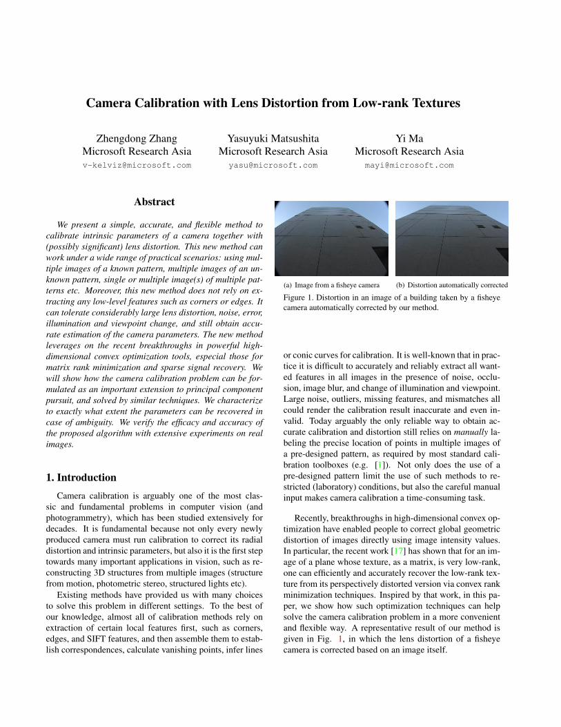
(a) Image from a fisheye camera (b) Distortion automatically corrected

Figure 1. Distortion in an image of a building taken by a fisheyecamera automatically corrected by our method.

or conic curves for calibration. It is well-known that in prac-tice it is difficult to accurately and reliably extract all want-ed features in all images in the presence of noise, occlu-sion, image blur, and change of illumination and viewpoint.Large noise, outliers, missing features, and mismatches allcould render the calibration result inaccurate and even in-valid. Today arguably the only reliable way to obtain ac-curate calibration and distortion still relies on manually la-beling the precise location of points in multiple images ofa pre-designed pattern, as required by most standard cali-bration toolboxes (e.g. [1]). Not only does the use of apre-designed pattern limit the use of such methods to re-stricted (laboratory) conditions, but also the careful manualinput makes camera calibration a time-consuming task.

Recently, breakthroughs in high-dimensional convex op-timization have enabled people to correct global geometricdistortion of images directly using image intensity values.In particular, the recent work [17] has shown that for an im-age of a plane whose texture, as a matrix, is very low-rank,one can efficiently and accurately recover the low-rank tex-ture from its perspectively distorted version via convex rankminimization techniques. Inspired by that work, in this pa-per, we show how such optimization techniques can helpsolve the camera calibration problem in a more convenientand flexible way. A representative result of our method isgiven in Fig. 1, in which the lens distortion of a fisheyecamera is corrected based on an image itself.

Contributions. In this paper, we will show that this newapproach leads to a simple and accurate solution to cameracalibration or self-calibration without requiring extracting,labeling, or matching any low-level features such as pointsand edges. The new algorithm directly works with raw im-age intensity values and can accurately estimate the cameraintrinsic parameters and lens distortion under a broad prac-tical conditions: from a single or multiple images, from aknown or unknown pattern, even with possible noise, sat-urations, occlusion, and under different illuminating condi-tions. It can be used either for pre-calibrating the camer-a from a known pattern or for performing automatic self-calibration from images of structured scenes. It requiresfew, inaccurate initialization, and thus is very convenien-t to use. Also, as it relies on scalable optimization tech-niques, with proper implementation, the speed can be veryfast. As we will verify with extensive experiments, the al-gorithm achieves comparable performance to the standardtoolbox, but with more flexible initialization and workingunder broader realistic conditions.

1.1. Prior work

During the past several decades, researchers have studiedmany different approaches for developing more convenient,practical, and accurate algorithms for camera calibration.

One important class of these solutions require a special-ly designed calibration object, with 3-D geometric informa-tion known explicitly [2, 6, 7, 14, 15]. The calibration ob-jects include 3-D [14], 2-D plane [15], and 1-D [16] line tar-gets. By observing these targets from different viewpoints,these techniques recover the camera intrinsic parameters.The 3-D calibration object usually consists of two or threeplanes orthogonal to each other, and it gives the most accu-rate calibration with a simple algorithm; however, the setupis more complicated and expensive. The 2-D plane-basedcalibration requires observing a planar pattern from differ-ent viewpoints. The technique is implemented in CameraCalibration Toolbox [1], and it gives accurate results withless complicated settings. The 1-D line-based calibrationuses a set of collinear points with known distances. Becauseit can better avoid occlusion problems, it is often used formulti-camera calibration.

Unlike above methods, camera self-calibration [11, 8]avoids the use of known calibration pattern and aims at cal-ibrating a camera by finding intrinsic parameters that areconsistent with the geometry of a given set of images. Itis understood that sufficient point correspondences amongthree images are sufficient to recover both intrinsic and ex-trinsic parameters. Because self-calibration relies on pointcorrespondences across images, it is important for these ap-proaches to extract accurate feature point locations and itnormally does not handle lens distortion.

Calibration based on vanishing points are also investigat-

ed by researchers [3, 10, 13, 4, 9]. These approaches utilizeparallelism and orthogonality among lines in the 3-D space.For example, certain camera intrinsics with the rotation ma-trix can be estimated from three mutually orthogonal van-ishing points. While useful, these approaches strongly relyon a process of edge detection and line fitting for accuratelydetermining vanishing points. Methods that use line fea-tures like done by Devernay and Faugeras [5] share similarprocesses, and the accuracy and robustness are too suscep-tible to noisy and faulty low-level feature extraction.

All in all, almost all calibration methods share one thingin common, i.e., almost exclusively relying on whetherpoints or lines can be reliably obtained from local corneror edge features. Feature extraction or labeling often be-comes a bottleneck of the process, affecting robustness, ac-curacy, and convenience. The proposed new method natu-rally avoids this problem by a new formulation that does notrequire any low-level feature extraction.

2. Camera Model with Lens Distortion

We first briefly describe the common mathematical mod-el used for camera calibration and introduce notation usedin this paper. We use a vector M = (X0, Y0, Z0)T ∈ R3

to denote the 3D coordinates of a point in the world co-ordinate frame, use mn = (xn, yn)T ∈ R2 to denote itsprojection on the canonical image plane in the camera co-ordinate frame. For convenience, we always denote the ho-mogeneous coordinate of a point m as m̃ = [m1 ].

Lens distortion model. If the lens of the camera is dis-torted, on the image plane, the coordinates of a point mn

may be transformed to a different one, denoted as md =(xd, yd)

T ∈ R2. A very commonly used general mathemat-ical model for this distortion D : mn 7→ md is given by apolynomial distortion model [2] by neglecting any higher-order terms as below:

r.=

√x2n + y2n,

f(r).= 1 + kc(1)r2 + kc(2)r4 + kc(5)r6, (1)

md =

[f(r)xn + 2kc(3)xnyn + kc(4)(r2 + 2x2n)f(r)xn + 2kc(4)xnyn + kc(3)(r2 + 2y2n)

].

Notice that this model has a total of five unknownskc(1), . . . , kc(5) ∈ R. If there is no distortion, simply setall kc(i) to be zero, and then it becomes md = mn.

Intrinsic parameters. To transform a point into the pixelcoordinates, we use the usual pin-hole model parametrizedby an intrinsic matrix K ∈ R3×3, which also have five un-knowns; the focal length along x and y-axes fx and fy ,skew parameter θ, and coordinates of the principle point

(ox, oy). In the matrix form, it is described as

K.=

fx θ ox0 fy oy0 0 1

∈ R3×3. (2)

Extrinsic parameters. Finally, we use R = [r1, r2, r3] ∈SO(3) and T ∈ R3 to denote the Euclidean transfor-mation from the world coordinate frame to the cameraframe – so-called extrinsic parameters. The rotation Rcan be parameterized by a vector ω = (ω1, ω2, ω3)T ∈R3 using the Rodrigues formula [7]: R(ω) = I +

sin ‖ω‖ ω̂‖ω‖ + (1 − cos ‖ω‖) ω̂2

‖ω‖2 , where ω̂ denotes the3 × 3 matrix form of the rotation vector ω, defined asω̂ = [0,−ω3, ω2;ω3, 0,−ω1;−ω2, ω1, 0] ∈ R3×3.

With all the notation, the overall imaging process of apoint M in the world to the camera pixel coordinates m bya pinhole camera can be describe as:

m̃ = Km̃d = KD(m̃n); λm̃n = [R T ]M̃, (3)

where λ is the depth of the point. If there is no lens dis-tortion (md = mn), the above model reduces the typicalpin-hole projection with an uncalibrated camera: λm̃ =K[R T ]M̃ .

For compact presentation, later in this paper, we will letτ0 denote the intrinsic parameters and lens distortion param-eters all together. We use τi (i = 1, 2, . . .) to denote the ex-trinsic parameters Ri and Ti for the i-th image. By a slightabuse of notation, we will occasionally use τ0 to representthe combined transformation of K and D acting on the im-age domain, i.e., τ0(·) = KD(·), and use τi (i = 1, 2, . . .)to represent the transforms from the world to individual im-age planes.

3. Calibration from Low-rank TexturesOur method estimates camera parameters from low-rank

textures. The pattern can be unknown, but is sufficient-ly structured, i.e., as a matrix it is sufficiently low-rank(e.g., the normally used checkerboard is one such pattern).We describe our method in two cases; multiple-image andsingle-image cases. From multiple observations of the low-rank textures, our method can fully recover lens distortion,intrinsics, and extrinsics. In the case of a single image asinput, our method can estimate lens distortion as well asintrinsics with additional yet reasonable assumptions.

By default we choose the origin of the world coordinateto be the top-left corner of the image and let the image lie inthe plane Z = 0 and X and Y be the horizontal and verticaldirection, respectively.

3.1. Multiple Images of the Same Low-Rank Pattern

Suppose we have images of a certain pattern I0 ∈Rm0×n0 taken from N different viewpoints R(ωi) and Ti

(in brief τi), with the same intrinsic matrix K and lens dis-tortion kc (in brief τ0). In practice, the observed images arenot direct transformed versions of I0, each may have con-tained some background or partially occluded regions (saydue to limited field of view of the camera). We use Ei tomodel such error between the original pattern I0 and the ithobserved image Ii with the transformations undone. Thenmathematically we have:

Ii ◦ (τ0, τi)−1 = I0 + Ei, (4)

where the operator ◦ denotes the geometric transformation-s. The task of camera calibration is then to recover τ0 andprobably τi (1 ≤ i ≤ N), too, from these images.

In general, we assume that we do not know I0 in ad-vance.1 So, we do not have any ground-truth pattern tocompare or correspond with for the images taken. Our goalis to fully recover the distortion and calibration by utilizingonly the low-rankness of the texture I0 and by establishingprecise correspondence among theN images Ii themselves.

Rectifying deformation via rank minimization. Wedraw inspiration from two previous work. Since we knowthe pattern is low-rank, from the work on transform invari-ant low-rank textures (TILT) [17], we can estimate the de-formation of each image Ii from I0 by solving the followingrobust rank-minimization problem:

min ‖Ai‖∗+λ‖Ei‖1, s.t. Ii ◦(τ0, τi)−1 = Ai+Ei, (5)

with Ai, Ei, τi and τ0 as unknowns. The work [17] hasshown that if there is no radial distortion in τ0, the aboveoptimization recovers the low-rank pattern I0 up to a trans-lation and scaling in each axis, i.e.,

Ai = I0 ◦ τ, where τ =[ sx 0 mx

0 sy my

0 0 1

]. (6)

However, in our problem, both intrinsic parameters and dis-tortion are present in the deformation. Therefore, a singleimage can no longer recover all the unknowns (and we willdiscuss in the next section exactly what can be recoveredfrom a single image of low-rank patterns.)

Our hope is that multiple images give us additional in-formation for all the unknown parameters. For that, weneed to establish precise point-to-point correspondence a-mong all the N images. Again, robust rank-minimizationtechniques offer a good guideline for solving this problem.In the previous work of RASL [12], the authors have pro-posed that multiple images can be precisely and efficientlyaligned by solving a robust rank-minimization problem sim-ilar to Eq. (5). However, the resulting aligned images could

1This is where our method deviates from the classical camera calibra-tion setting and it makes our method works under broader conditions. Wewill discuss by the end of the section what if we do know the pattern inadvance.

still differ from the canonical view I0 by an arbitrary lineartransformation, and each individual image as a matrix doesnot need to be low-rank.

Simultaneous alignment and rectification. For calibra-tion, we need to align all the N images point-wise, and atthe same time each resulting image should be rectified asa low-rank texture. Or more precisely, we want to find thetransformation τ ′0, τ

′i such that Ii, 1 ≤ i ≤ N can be ex-

pressed asIi ◦ (τ ′0 ◦ τ ′i)−1 = Ai + Ei,

where all Ai are low-rank and equal to each other Ai = Aj .Therefore, the natural optimization problem associated withthis problem becomes

min

N∑i=1

‖Ai‖∗ + ‖Ei‖1,

s.t. Ii ◦ (τ ′0 ◦ τ ′i)−1 = Ai + Ei, Ai = Aj . (7)

One can use optimization techniques similar to that ofTILT and RASL to solve the above optimization problem,such as the Alternating Direction Method (ADM) used in[17]. However, having too many constraining terms affectsthe convergence of these algorithms. In addition, in prac-tice, due to different illumination and exposure time, the Nimages could differ from each other in intensity and con-trast. Hence, in this paper, we propose an alternative, moreeffective and efficient way to align the images in the desiredway. The idea is to concatenate all the images as submatri-ces of a joint low-rank matrix:

D1.= [A1, A2, . . . , AN ], D2

.= [AT1 , A

T2 , . . . , A

TN ],

E.= [E1, E2, . . . , EN ]. (8)

We try to simultaneously align the columns and rows ofAi and minimize its rank by solving the following problem:

min ‖D1‖∗ + ‖D2‖∗ + λ‖E‖1,s.t. Ii ◦ (τ0 ◦ τi)−1 = Ai + Ei, (9)

with Ai, Ei, τ0, τi as unknowns. Notice that, by comparingto Eq. (7), which introduces inN+ N(N−1)

2 constraints, thenew optimization has just N constraints and hence is easierto solve. In addition, it is insensitive to illumination andcontrast change across different images. One may view theabove optimization as a generalization for both TILT andRASL: When N = 1, it reduces to TILT; and when there isno D2, this reduces to something similar to RASL.

To deal with the nonlinear constraints in Eq. (9), welinearize the constraints Ii ◦ (τ0, τi)

−1 = Ai + Ei w.r.tall the unknown parameters τ0, τi. To reduce the effec-t of change in illumination and contrast, we normalize

Algorithm 1 (Align Low-rank Textures for Calibration).Input: A rectangular window Ii ∈ Rmi×ni in each im-age, initial extrinsic parameter τi, common intrinsic andlens distortion parameters τ0, and weight λ > 0.While not converged Do

step 1: for each image, normalize it and computethe Jacobian w.r.t. unknown parameters:

Ii ◦ (τ0, τi)−1 ← Ii ◦ (τ0, τi)

−1

‖Ii ◦ (τ0, τi)−1‖F

;

J0i ←

∂

∂ζ0

(Ii ◦ (ζ0, ζi)

−1

‖Ii ◦ (ζ0, ζi)−1‖F

)∣∣∣ζ0=τ0,ζi=τi

;

J1i ←

∂

∂ζi

(Ii ◦ (ζ0, ζi)

−1

‖Ii ◦ (ζ0, ζi)−1‖F

)∣∣∣ζi=τi,ζ0=τ0

;

step 2: solve the linearized convex optimization:min ‖D1‖∗ + ‖D2‖∗ + λ‖E‖1,s.t. Ii ◦ (τ0, τi)

−1 + J0i ∆τ0 + J1

i ∆τi = Ai + Ei;

step 3: update: τ0 ← τ0 + ∆τ0, τi ← τi + ∆τi;End WhileOutput: Converged solution τi, τ0.

Ii ◦ (τ0, τi)−1 by its Frobenius norm to Ii◦(τ0◦τi)−1

‖Ii◦(τ0◦τi)−1‖F . Let

J0i = ∂

∂τ0

(Ii◦(τ0◦τi)−1

‖Ii◦(τ0◦τi)−1‖F

)be the Jacobian of the normal-

ized image w.r.t. shared intrinsic and distortion parametersτ0 and J1

i = ∂∂τi

(Ii◦(τ0◦τi)−1

‖Ii◦(τ0◦τi)−1‖F

)be the Jacobian w.r.t

extrinsic parameters τi for each image. The local linearizedversion of Eq. (9) becomes

min ‖D1‖∗ + ‖D2‖∗ + λ‖E‖1,s.t. Ii ◦ (τ0, τi)

−1 + J0i ∆τ0 + J1

i ∆τi = Ai + Ei, (10)

with ∆τ0,∆τi, Ai, Ei as unknowns. Notice that this lin-earized problem is a convex optimization problem andcan be efficiently solved by some of the modern high-dimensional optimization methods such as the ADMmethod mentioned earlier. To find the global solution to theoriginal nonlinear problem Eq. (9), we only have to incre-mentally update τ0 and τi by ∆τ0,∆τi and iteratively rerunthe above program until convergence. The overall algorithmis summarized in Algorithm 1.

In general, as long as there is sufficient textural variationin the pattern, the lens distortion parameters kc can alwaysbe accurately estimated by the algorithm once the low-ranktexture of the pattern is fully rectified. This is the case evenfrom a single image2.

Now the remaining question is, under what conditionsthe correct intrinsic parametersK and the extrinsic parame-

2although a rigorous mathematical proof for this fact is beyond the s-cope of this paper.

ters (Ri, Ti) are the global minimum to the problem Eq. (9),and whether there is still some ambiguity.

Proposition 1. Given N ≥ 5 images of the low-rank pat-tern I0 taken by a camera with the same intrinsic param-eters K under generic viewpoints τi = (Ri, Ti): Ii =I0 ◦ (τ0 ◦ τi), i = 1, . . . , N . Then the optimal solution(K ′, τ ′i) to problem Eq. (9) must satisfy K ′ = K andR′i = Ri.

That is, all the distortion and intrinsic parameters τ0 canbe recovered and so is the rotation Ri of each image. Thereis only ambiguity left in the recovered translation Ti ofeach image. The proof is rather routine based on existingwork on cameral calibration, but for completeness, a de-tailed derivation is given in Appendix A as supplementarymaterial to this paper.

With a known pattern. If the ground-truth I0 is giv-en and its metric is known, then we may want to alignIi to I0 directly or indirectly. One possible solution isto slightly modify Algorithm 1 by appending D1, D2, Ewith A0, A

T0 , E0, respectively, and adding the constrain-

t I0 = A0 + E0. Another possible solution would be toalign the already rectified textures Ai to I0 by maximizingthe correlation.

In both situations, with knowledge about the metric ofI0, we can uniquely determine Ti and get exactly the full setof intrinsic and extrinsic parameters. Technical justificationis given in Appendix B of the supplementary material.

3.2. Self-Calibration from a Single Image

With a single plane. For most everyday usage of a cam-era, people normally do not need to know the full intrinsicparameters of the camera. For instance, for webcam users,it normally suffices if we can simply remove the annoyinglens distortion. For such users, asking them to take multi-ple images and conduct a full calibration might be too muchtrouble. Sometimes, we need to remove the radial distortionof an image but without any access to the camera itself.

Therefore, it would be desirable if we can calibrate thelens distortion of a camera from a single image. Normallythis would be impossible for a generic image. Nevertheless,if the image contains a plane with low-rank pattern rich withhorizontal and vertical lines, then the lens distortion kc canbe correctly recovered using our method.

Given a single image with a single low-rank pattern, s-ince we cannot expect to obtain all the intrinsic parame-ters correctly, we can make the following simplifying as-sumptions about K: No skew θ = 0, principal point known(say set at the center of the image), and pixel being square(fx = fy = f ). Although these seem to be somewhat re-strictive, they approximately hold for many cameras made

today. In this circumstance, if the viewpoint is not degener-ate, applying the algorithm to the image of this single pat-tern correctly recovers the lens distortion parameters kc andthe focal length f .

With two orthogonal planes. Very often, an image con-tains more than one planar low-rank textures, and they sat-isfy additional geometric constraints. For instance, in a typ-ical urban scene, an image often contains two (orthogonal)facades of a building. Each facade is full of horizontal andvertical lines and can be considered as a low-rank texture.In this case, the image encodes much richer informationabout the camera calibration: Both the focal length and theprincipal point can be recovered from such an image, giventhat the pixel of the camera is assumed to be square, i.e.,fx = fy = f , and there’s no skew, i.e., θ = 0.

For simplicity, we let the intersection of these two or-thogonal planes be the z-axis of the world frame, and thetwo planes are x = 0 and y = 0, each with a low-rank tex-ture I(i)0 , i = 1, 2. We take a photo of the two planes by acamera with intrinsic parameters K and lens distortion kc,from the viewpoint (R, T ). Denote the photo as I , whichcontains two mutually orthogonal low-rank patterns.

Let ML = [0 Y1 Z1]T ∈ R3 be a point on the leftfacade, and MR = [X2 0 Z2]T ∈ R3 be a point on theright facade, and let mL,mR ∈ R2 be the correspondingimages on I . Then we have:

λ1m̃L =

[f 0 ox0 f oy0 0 1

][r2 r3 T1]

[Y1

Z11

], (11)

and

λ2m̃R =

[f 0 ox0 f oy0 0 1

][r1 r3 T2]

[X2

Z21

]. (12)

Here we have used a different translation T1 or T2 for eachplane, mainly because otherwise we must exactly find theposition of the intersection of the two planes, which is be-yond the scope of this paper. So in this circumstance letτ0 = [f, ox, oy, kc(1 : 5), ω] and τi = [Ti] and the opti-mization problem we need to solve to recover them is:

minAi,Ei,τ0,τi ‖A1‖∗ + ‖A2‖∗ + λ(‖E1‖1 + ‖E2‖1),

subject to I ◦ (τ0, τi)−1 = Ai + Ei. (13)

With similar normalization and linearization techniques, wecan solve this problem with slight modification to Algorith-m 1.

Proposition 2. Given one image of two orthogonal planeswith low-rank textures, taken by a camera from a gener-ic viewpoint (R, T ) with intrinsic parameters K with zerosskew θ = 0 and square pixels(fx = fy). If K ′, R′, T ′1, T

′2

are solutions to problem Eq. (13), then K ′ = K, R′ = R.

By an argument similar to the multiple-image case, torecover τ0, we only need to rectify the left and right tex-tures with a joint parameterization of the rotation. For com-pleteness, we leave detailed analysis in Appendix C of thesupplementary material and shows that the solution for τ0 isindeed the correct one.

3.3. Implementation

Detection of the pattern. The initialization of our algo-rithm is extremely simple and flexible. The location ofthe initial window can be obtained from any segmentationmethods that approximately detect the region of the pattern.Or it can be easily specified by a human. There is no needfor the location of the initial window to be exact or evencover the pattern region. The proposed method is very ro-bust and can converge precisely to the pattern.

Initialization. We can first run the TILT on each initialwindow to approximately extract the homography Hi forthe ith image. Then we can obtain a rough estimate ofK,R, T as from the vanishing points given by the first t-wo columns of τi.3 For lens parameters, even if large lensdistortion is present, we set their initial values to be zero.

Multi-resolution implementation. To make the conver-gence region of our algorithm large and to accelerate the al-gorithm, we employ the conventional multi-resolution im-plementation with a proper blurring and pyramid scheme,similar to that described in the work on TILT [17].

4. Simulations and Experiments4.1. Calibration from Multiple Images

A. Calibration using a known pattern. In this experi-ment, we compare our proposed method with the standardcamera calibration toolbox [1]. Normally, the error of cal-ibration can be evaluated by reprojection error of extractedfeature points. But since our method does not involve anyfeature extraction and uses only the raw image pixels, thismeasurement of error is no longer suitable here. Instead, wetry to compare the accuracy of estimated camera parametersagainst the average estimates. More precisely, we run mul-tiple experiments with different images by the same cameraand compute the standard deviation for every parameter weestimate. The smaller the deviation, the more stable the es-timates are.

In this experiment, we take 50 photos of a knownchecker-board pattern using the same camera and setting,from different viewpoints. In each experiment, we ran-domly select 20 out of the 50 images. With these select-ed images, we calibrate the camera with both the proposed

3It is easy to see that the first two columns of τi correspond to thevertical and horizontal directions of the low-rank textures.

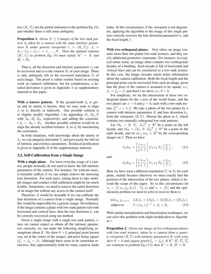
(a) Initialization for the Toolbox (b) Initialization of Our Method

Figure 2. Representative examples of initialization for the twomethods. Notice that ours can be very flexible.

(a) Comparison of intrinsic parameters (b) Comparison of distortion parameters

Figure 3. Comparison with the standard calibration toolbox. Stan-dard deviation in the estimated parameters, in pixels.

method and the standard toolbox. Note that we need to man-ually click the precise location of the four corners of thechecker-board for the toolbox. But for our method, the ini-tialization needs not to be exact at all (several pixels away).See Figure 2 for examples. We repeat the experiment 20times, and calculate the standard derivation of each param-eter4 for each method. The result is shown in Figure 3.

From the figure, we can see that our method is more sen-sitive in the estimation of focal length and principle pointsthan toolbox, but the performance is comparable.5 The es-timation of lens-distortion parameters of our method is al-most the same as the toolbox.

So to conclude from this experiment, under noise-free,well-controlled conditions, the performance of our methodis quite comparable to the toolbox. But our method doesnot require exact initialization of the point location. In laterexperiments, we will see that our method can work undermuch broader conditions: with an unknown pattern, froma single image, and even when significant lens distortionexists, such as fish-eye images.

In order to verify the accuracy of the remaining experi-ments, unless otherwise stated, we use the same Panasoniccamera with the same image resolution [960, 540] (directly

4 By default the calibration toolbox disables the estimation of skew.When turned on, it gives an error. So in this comparison, we do not esti-mate skew either although our method does not have this limitation.

5No serious attempt has been made to improve the numerical stabilityof our method. We believe this sensitivity can be easily addressed by amore careful numerical implementation in the future.

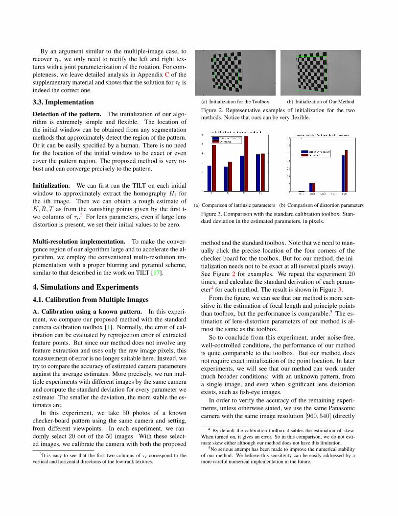
(a) Input images and windows (b) Rectified and aligned textures

Figure 4. Camera calibration from images of an unknown pat-tern. The algorithm aligns the low-rank textures precisely despitespecularities in the images. Although aligned and rectified, corre-sponding pixels do not have to correspond to the same 3D point.

down-sampled from its full [1920, 1080] resolution). Thecamera parameters estimated from this experiment is:

K =[

1142.0 0 453.70 1136.5 301.20 0 1

]. (14)

The camera should have the same set of parameters, exceptfor focal length which may change from experiment to ex-periment.

B. Calibration from an unknown pattern. In this exper-iment, we take multiple photos of an unknown mosaic wallfrom different viewpoints. By rectifying and aligning themosaic images pixel-wise into a common canonical frame,as shown in Figure 4, we obtain the camera calibration. Therecovered intrinsic matrix is:

K̂ =[

1138.6 0 482.30 1127.8 267.70 0 1

]. (15)

4.2. Calibration from a Single Image

C. Calibration from a single pattern. Given just a sin-gle image or a regular pattern, to calibrate the camera, wehave to work with fairly strong assumptions, say that theprincipal point is known (and simply set as the center of theimage) and the pixel is square. Then from the image, onecan calibrate the focal length as well as eliminating the lensdistortion. Figure 5 shows an example with an image givenin the standard toolbox. The estimated intrinsic parameter-s K̂ and the ground-truth K (provided by the calibrationtoolbox) are respectively:[677.1812 0 319.5000

0 677.1812 239.50000 0 1

],[661.6700 0 306.0959

0 662.8285 240.789870 0 1

].

The small error in focal length is mainly due to that theprinciple point is approximated with the center of the image.Nevertheless, we see in Figure 5(b), the radial distortion iscompletely removed by our algorithm.

(a) Input image and window (b) Radial distortion removed

Figure 5. Calibration from a single image in the Toolbox.

(a) Input image (b) Rectified texture

Figure 6. Calibration of our camera using an image of this paper.

To show the flexibility of our method, we further showanother example in Figure 6 where we took with the Pana-sonic camera an image of the frontal page of this paper.With this image as input, the recovered calibration matrixis:

K̂ =[1229.1 0 479.5

0 1229.1 269.50 0 1

]. (16)

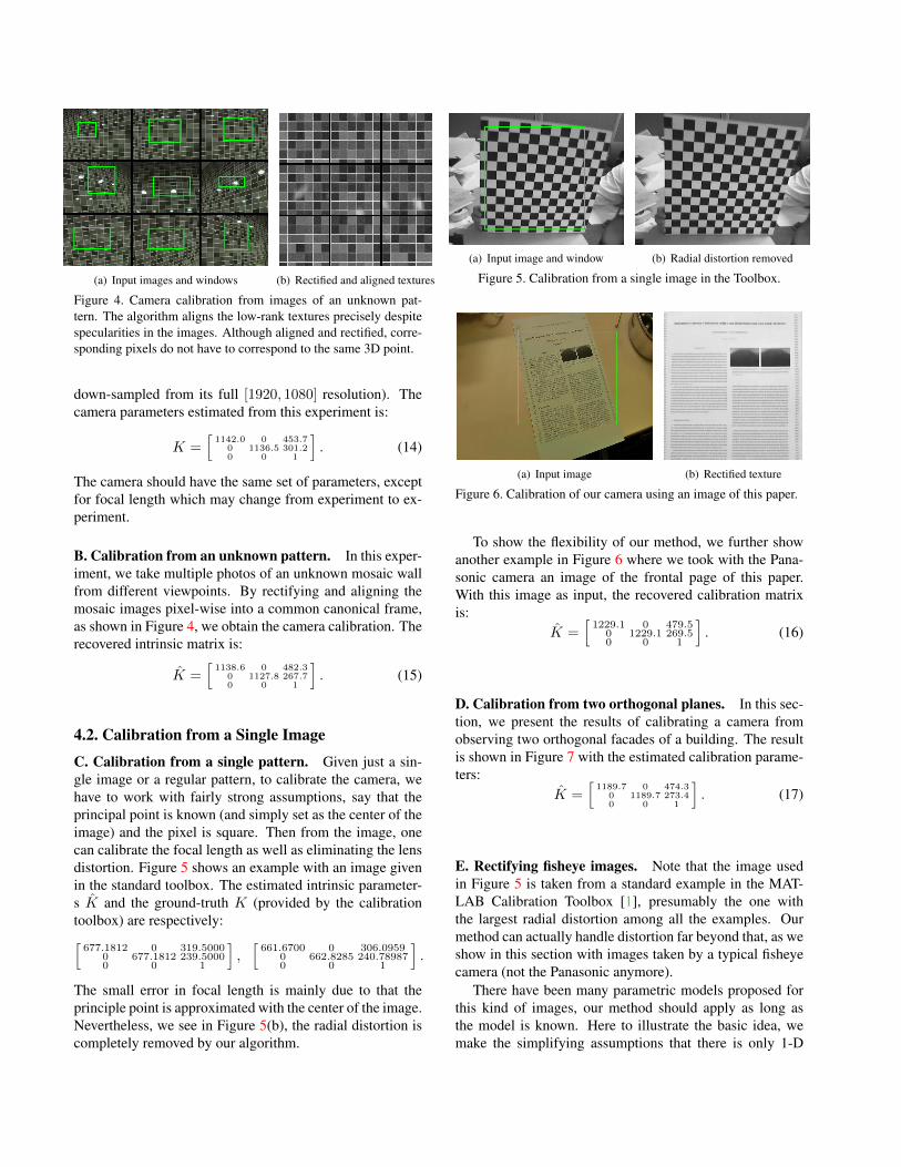
D. Calibration from two orthogonal planes. In this sec-tion, we present the results of calibrating a camera fromobserving two orthogonal facades of a building. The resultis shown in Figure 7 with the estimated calibration parame-ters:

K̂ =[

1189.7 0 474.30 1189.7 273.40 0 1

]. (17)

E. Rectifying fisheye images. Note that the image usedin Figure 5 is taken from a standard example in the MAT-LAB Calibration Toolbox [1], presumably the one withthe largest radial distortion among all the examples. Ourmethod can actually handle distortion far beyond that, as weshow in this section with images taken by a typical fisheyecamera (not the Panasonic anymore).

There have been many parametric models proposed forthis kind of images, our method should apply as long asthe model is known. Here to illustrate the basic idea, wemake the simplifying assumptions that there is only 1-D

(a) Input image (b) Rectified image

(c) Rectified texture of left facade (d) Rectified texture of right facade

Figure 7. Calibration from two orthogonal facades of a building.

Figure 8. Rectify fisheye images with significant lens distortion.Top: input images with a selected window (red); Middle: rectifiedimages; Bottom: rectified low-rank textures (from green window).

distortion along the radial direction and hence try to esti-mate the mapping along the radius before and after distor-tion r = f(rd). We approximate f(·) by polynomials upto degree 4. In addition, we assume the center of the dis-tortion is the center of the image. Moreover, since no priorknowledge about K,R, T is available, we model the trans-formation from the pattern to the image plane as a generalhomography transformation H ∈ R3×3. Some representa-tive results are shown in Figure 8.

References[1] J.-Y. Bouguet. Camera calibration toolbox for Matlab.

http://www.vision.caltech.edu/bouguetj/calib_doc/. 1, 2, 6, 7

[2] D. Brown. Close-range camera calibration. Photogrammet-ric Engineering, 37(8):855–866, 1971. 2

[3] B. Caprile and V. Torre. Using vanishing points for cameracalibration. IJCV, 4(2):127–140, Mar 1990. 2

[4] R. Cipolla, T. Drummond, and D. Robertson. Camera cal-ibration from vanishing points in images of architecturalscenes. In BMVC, volume 2, pages 382–391, 1999. 2

[5] F. Devernay and O. D. Faugeras. Automatic calibrationand removal of distortion from scenes of structured environ-ments. In SPIE Conference on Investigative and Trial ImageProcessing, volume 2567, pages 62–72, 1995. 2

[6] W. Faig. Calibration of close-range photogrammetry system-s: Mathematical formulation. Photogrammetric Engineeringand Remote Sensing, 41(12):1479–1486, 1975. 2

[7] O. Faugeras. Three-Dimensional Computer Vision: a Geo-metric Viewpoint. MIT Press, 1993. 2, 3

[8] O. Faugeras, Q. Luong, and S. Maybank. Camera self-calibration: Theory and experiments. In ECCV, pages 321–334, 1992. 2

[9] L. Grammatikopoulos, G. Karras, E. Petsa, and I. Kalisper-akis. A unified approach for automatic camera calibrationfrom vanishing points. International Archives of the Pho-togrammetry, Remote Sensing & Spatial Information Sci-ences, XXXVI(5), 2006. 2

[10] D. Liebowitz and A. Zisserman. Metric rectification for per-spective images of planes. In CVPR, pages 482–488, June1998. 2

[11] S. Maybank and O. Faugeras. A theory of self-calibration ofa moving camera. IJCV, 8(2):123–152, Aug. 1992. 2

[12] Y. Peng, A. Ganesh, J. Wright, W. Xu, and Y. Ma. RASL:Robust alignment by sparse and low-rank decomposition forlinearly correlated images. In CVPR, 2010. 3

[13] P. Sturm and S. J. Maybank. A method for interactive 3D re-construction of piecewise planar objects from single images.In In BMVC, 1999. 2

[14] R. Tsai. A versatile camera calibration technique for high-accuracy 3D machine vision metrology using off-the-shelf tvcameras and lenses. IEEE Journal of Robotics and Automa-tion, 3(4):323–344, Aug. 1987. 2

[15] Z. Zhang. Flexible camera calibration by viewing a planefrom unknown orientations. In ICCV, 1999. 2

[16] Z. Zhang. Camera calibration with one-dimensional objects.PAMI, 26(7):892 –899, 2004. 2

[17] Z. Zhang, X. Liang, A. Ganesh, and Y. Ma. TILT: Transforminvariant low-rank textures. In ACCV, 2010. 1, 3, 4, 6

Supplementary Material

A. Proof of Proposition 1: Ambiguities in Cal-ibration with an Unknown Pattern

Proof. Suppose by solving Eq. (9), we have aligned all theimages up to translation and scaling of I0. To be more spe-cific we have managed to find τ ′i = (R′i, T

′i ), τ

′0 = (K ′, k′c)

such that

Ii ◦ (τ ′0 ◦ τ ′i)−1 = I0 ◦ τ, with τ =

sx 0 mx

0 sy my

0 0 1

.As all the lines have become straight in the recovered im-ages Ai, the radial distortion parameters k′c should be exactk′c = kc.

Here sx, sy are scaling in the x and y directions of thealigned images Ai w.r.t. the original low-rank pattern I0.mx and my are the translations between Ai and I0. Now letus consider the mapping between a point M0 on I0 (noticethat the Z-coordinate is zero by default) and its image m̃ ∈R3 (in homogeneous coordinates): λm̃ = K[r1, r2, T ]M0.As the recovered parameters are consistent with all con-straints, the same point and its image satisfy:

λ′m̃ = K ′[r′1, r′2, T

′]

sx 0 mx

0 sy my

0 0 1

M0.

So the matrix K[r1, r2, T ] must be equivalent toK ′[sxr

′1, syr

′2,mxr

′1+myr

′2+T ′] (i.e., up to a scale factor),

so we have{Kr1 = ξsxK

′r′1,Kr2 = ξsyK

′r′2.⇒{K ′−1Kr1 = ξsxr

′1,

K ′−1Kr2 = ξsyr′2.

(18)

Since r′T1 r′2 = 0, we have

(Kr1)TK ′−TK ′−1(Kr2) = 0. (19)

This gives one linear constraint for B = K ′−TK ′−1. Sucha symmetric B has six degrees of freedom. Since each im-age gives one constraint on B, we need only five generalimages (not in degenerate configurations) to recover B upto a scale. Since K−TK−1 is a solution too, thus we musthave K ′ = K as the unique solution of the form Eq. (2).Further from Eq. (18), we have r′1 = r1, r′2 = r2, andsx = sy . That is, once all the images are aligned and recti-fied, they only differ from the original pattern I0 by a globalscale s = sx = sy and a translation (mx,my). In addition,we recovered rotation R′i is the correct R′i = Ri. But sincewe still do not know the exact values of sx, mx, and my ,the recovered T ′i is not necessarily the correct Ti.

With a similar analysis, we can show that in fact if we in-dividually rectify the images, we still can obtain the correctK and Ri. The only difference is that sx, sy , mx and my

are all different for different images, thus the translations Tiare even less constrained.

B. Determine Translation from Ground-TruthIf the low-rank pattern I0 is given, we can directly or

indirectly align Ii to I0. From a derivation similar to theabove, one can show that we can recover sx, mx and my

with respect to the ground truth metric of I0. Then for eachimage the ground-truth translation can be recovered by

T =mxr1 +myr2 + T ′

sx. (20)

C. Proof of Proposition 2: Ambiguities in Cal-ibration with Two Orthogonal Planes

Proof. Suppose a low-rank texture lies on the left planeX = 0 and another lies on the right plane Y = 0.ML = (0, Y1, Z1) is the point on the left plane, andMR = (X2, 0, Z2) is a point on the right plane. Similar-ly we have the image point mL = (xL, yL) of the left pointand mR = (xR, yR) of the right point. Then

λ1mL =

f 0 ox0 f oy0 0 1

[r2 r3 T ]

Y1Z1

1

, (21)

and

λ2mR =

f 0 ox0 f oy0 0 1

[r1 r3 T ]

X2

Z2

1

. (22)

For convenience, we use (x, y) to represent points bothon Y = 0 and on X = 0. Suppose the rectified im-age Ai differs from the ground truth I

(i)0 by scaling and

translation: s(i)x , s(i)y ,m

(i)x ,m

(i)y . Then the ground truth K,

R = [r1 r2 r3] and T , and the recovered parameters K ′,R′ = [r′1 r

′2 r′3] and T ′1, T

′2 are related through the following

formulae:[s(1)x Kr2 s

(1)y Kr3 K(m

(1)x r2 +m

(1)y r3 + T )

]= ξ1 [K ′r′2 K ′r′3 K ′T ′1] ,[s(2)x Kr1 s

(2)y Kr3 K(m

(2)x r1 +m

(2)y r3 + T )

]= ξ2 [K ′r′1 K ′r′3 K ′T ′2] .

(23)

This gives

K ′−1K[s(2)xξ2

r1,s(1)x

ξ1r2,

s(1)y

ξ1r3

]= [r′1, r

′2, r

′3]. (24)

Knowing that r′1, r′2, r′3 are orthogonal to each other, we de-

rive three linear constraints for B = K ′−TK ′−1, which hasthree unknowns. So in general, we can extract unique so-lution K ′ from B. Note that K ′ = K is one solution too,hence the recovered is the correct solution.

Also, from Eq. (24) we can see that R′ = R, leavingonly Ti being ambiguous.