Can earnings manipulation create value?�

Anton Migloy

January 2008

�I would like to thank Claude Fluet, Hikmet Gunet, Pierre Lasserre, Nicolas Marceau,Michel Robe, and the seminar and conference participants at UQAM, the 2006 FMAmeeting, the 2005 FMA European meeting, the 2005 Swiss Financial Market Associationmeeting, the 2005 Western Economics Association International meeting, the 2003 Cana-dian Economics Association meeting, and the 2003 French Finance Association meetingfor their helpful discussions and comments. I am also thankful for the �nancial supportawarded by the Social Sciences and Humanities Research Council of Canada (SSHRC) andthe Institut de �nance mathématique de Montréal.

yAuthor a¢ liation and manuscript correspondence: University of Guelph, Departmentof Economics, Guelph, Ontario, Canada, N1G 2W1, tel. (519) 824-4120 ext. 53054, email:amiglo@uoguelph.ca.

1

Can earnings manipulation create value?Abstract. Existing literature usually considers earnings manipulation to

be a negative social phenomenon. We argue that earnings manipulation canbe a part of the equilibrium relationships between �rms�insiders and out-siders. We consider an optimal contract between an entrepreneur and aninvestor where the entrepreneur is subject to a double moral hazard problem(one being the choice of production e¤ort and the other being intertemporalsubstitution, which consists of transferring cash �ows between periods). In-vestment and production e¤ort may be below socially optimal levels becausethe entrepreneur cannot entirely capture the results of his e¤ort. The oppor-tunity to manipulate earnings protects the entrepreneur against the risk ofa low payo¤ when the results of production are low. Ex-ante, this providesan incentive for the entrepreneur to increase his level of e¤ort and investe¢ ciently.

Key words: earnings manipulation, intertemporal substitution, design ofsecurities, property rights, moral hazardJEL classi�cation codes: G32, D92, D82

2

1 Introduction.

The recent wave of corporate scandals (Worldcom, Enron, Nortel etc.) hasraised heated debates regarding the manipulation of earnings by �rms�in-siders. Existing literature usually considers earnings manipulation (hereafterEM) to be a negative social phenomenon and suggests measures for its elim-ination. In the present paper, we argue that earnings manipulation can be apart of the equilibrium relationships between �rms�insiders and outsiders.In contrast to earnings being misreported, which in most cases represents

accounting fraud,1 we consider EM to be a transfer of funds between peri-ods. This transfer does not create any social value (in contrast to productivee¤ort). Some typical examples include delaying the approval of importantdecisions, ine¢ cient investments, borrowing in order to manipulate �nancialresults, ine¢ cient discount policy etc.2 EM is well documented in empiricalliterature. For instance, Degeorge, Patel, and Zeckhauser (1999) discovereddiscontinuities in the distribution of corporate earnings at some speci�c val-ues (thresholds). The number of reports with earnings just below the thresh-old is much lower than those just above the threshold. This suggests thatinsiders are involved in earnings manipulation around the threshold level.Burgstahler and Dichev (1997) show that 30-44% of �rms with small pre-managed losses manage earnings to create a positive pro�t. Recently, Yu,Du, and Sun (2004) examined earnings management by Chinese �rms andfound earnings manipulation around two thresholds.Degeorge, Patel, and Zeckhauser (1999) also present a theoretical model

involving EM by a manager with a bonus-like contract. The authors showthat the manager�s incentive to manipulate earnings depends on the values ofthe latent (pre-managed) earnings, the manager�s bonus, and the magnitudeof the social loss from EM. The manager�s decision also relies on whether pre-

1For empirical evidence about earnings misreporting see Dechow, Sloan and Sweeney(1996) and Erickson, Hanlon and Maydew (2003). For theoretical papers see Cornelli andYoscha (2003), Crocker and Slemrod (2005) and Johnsen and Talley (2005).

2Other examples include the choice of inventory methods, allowance for bad debt, ex-pensing of research and development, recognition of sales not yet shipped, estimation ofpension liabilities, capitalization of leases and marketing expenses, and delay in main-tenance expenditures (see Degeorge, Patel and Zeckhauser, 1999). Roychowdhury (2006)provides extensive evidence on earnings management through real activities manipulation.

3

dictions of future pro�ts are certain or risky. In contrast, the model in thepresent paper contains a double-moral hazard problem (one being the choiceof production e¤ort and the other being the EM decision). We compare dif-ferent contractual arrangements between an investor and an entrepreneur aswell as their impact on the entrepreneur�s e¤ort. This is important given thatseveral recent papers analyze the links between �nancing structures and EM(see, for instance, Richardson, Tuna and Wu (2007), Hodgson and Stevenson(2000) and Jensen (2002)). Finally, we compare the model�s predictions withEM and without EM.We analyze a model where a �rm needs external �nancing. The �rm�s

value consists of current (�rst-period) earnings and the going concern value.In contrast to current earnings, it is costly to verify the going concern valueof the �rm and enforce payments contingent on it (for instance, since itis impossible to describe all states of nature in the future and all optimalactions, the �rm�s owners may be able to divert all future earnings to theirown pockets).3 The fact that it is impossible to write a complete contractcontingent on the �rm�s going concern value eliminates any opportunity towrite a contract contingent on the �rm�s total value (which would eliminatethe problem of EM because EM cannot increase the �rm�s total value). The�nancing contract includes cash payments and an allocation of rights on the�rm�s going concern value - both being contingent on the magnitude of the�rm�s current earnings.4 The contract may optimize the value of the partiescooperation because of the impact it has on the entrepreneur�s incentives toprovide productive e¤ort and engage in EM. For instance, if the going concernvalue represents a new �rm and the party responsible for decision-making isthe sole owner of this new �rm, this party will be interested in shifting thevalue of the original business to the new �rm (even if it is socially ine¢ cient).As mentioned above, we compare two situations. In the �rst, the entrepre-

neur chooses only a costly productive e¤ort - assuming that the entrepreneurcannot be involved in EM. In the second, the entrepreneur is subject to adouble-moral hazard problem which includes the choice of productive e¤ortand the EM decision. It is shown that the entrepreneur�s productive e¤ortmay be higher in the second case. The following demonstrates the intuitionsbehind this result. Consider debt �nancing. If current earnings are below the

3For a similar approach see, for example, Hart, 1995.4See, among others, Kaplan and Stromberg (2004) for contingencies in �nancing con-

tracts.

4

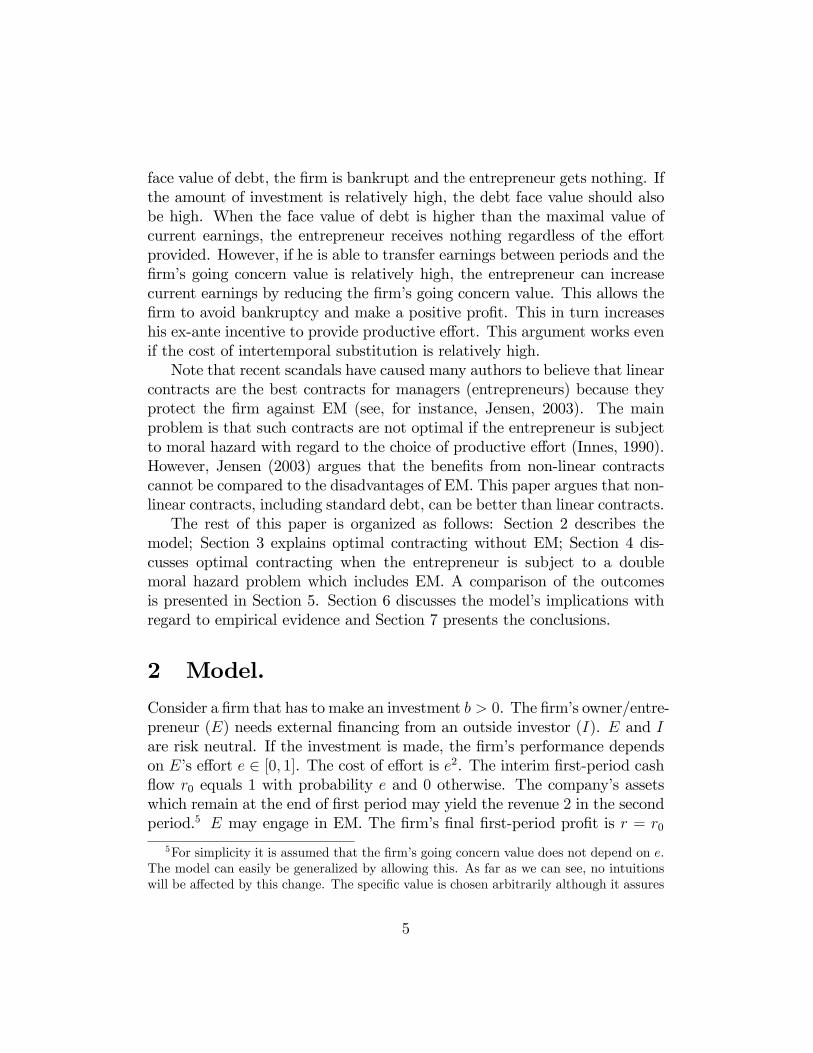
face value of debt, the �rm is bankrupt and the entrepreneur gets nothing. Ifthe amount of investment is relatively high, the debt face value should alsobe high. When the face value of debt is higher than the maximal value ofcurrent earnings, the entrepreneur receives nothing regardless of the e¤ortprovided. However, if he is able to transfer earnings between periods and the�rm�s going concern value is relatively high, the entrepreneur can increasecurrent earnings by reducing the �rm�s going concern value. This allows the�rm to avoid bankruptcy and make a positive pro�t. This in turn increaseshis ex-ante incentive to provide productive e¤ort. This argument works evenif the cost of intertemporal substitution is relatively high.Note that recent scandals have caused many authors to believe that linear

contracts are the best contracts for managers (entrepreneurs) because theyprotect the �rm against EM (see, for instance, Jensen, 2003). The mainproblem is that such contracts are not optimal if the entrepreneur is subjectto moral hazard with regard to the choice of productive e¤ort (Innes, 1990).However, Jensen (2003) argues that the bene�ts from non-linear contractscannot be compared to the disadvantages of EM. This paper argues that non-linear contracts, including standard debt, can be better than linear contracts.The rest of this paper is organized as follows: Section 2 describes the

model; Section 3 explains optimal contracting without EM; Section 4 dis-cusses optimal contracting when the entrepreneur is subject to a doublemoral hazard problem which includes EM. A comparison of the outcomesis presented in Section 5. Section 6 discusses the model�s implications withregard to empirical evidence and Section 7 presents the conclusions.

2 Model.

Consider a �rm that has to make an investment b > 0. The �rm�s owner/entre-preneur (E) needs external �nancing from an outside investor (I). E and Iare risk neutral. If the investment is made, the �rm�s performance dependson E�s e¤ort e 2 [0; 1]. The cost of e¤ort is e2. The interim �rst-period cash�ow r0 equals 1 with probability e and 0 otherwise. The company�s assetswhich remain at the end of �rst period may yield the revenue 2 in the secondperiod.5 E may engage in EM. The �rm�s �nal �rst-period pro�t is r = r0

5For simplicity it is assumed that the �rm�s going concern value does not depend on e.The model can easily be generalized by allowing this. As far as we can see, no intuitionswill be a¤ected by this change. The speci�c value is chosen arbitrarily although it assures

5

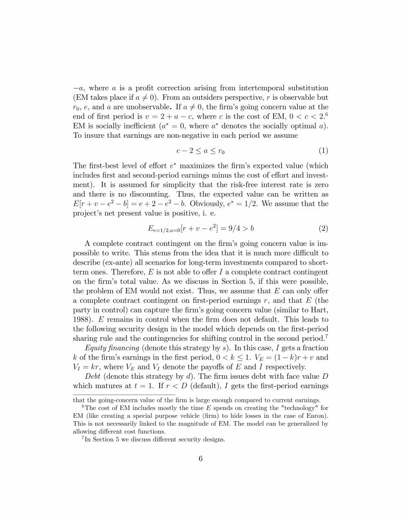
�a, where a is a pro�t correction arising from intertemporal substitution(EM takes place if a 6= 0). From an outsiders perspective, r is observable butr0, e, and a are unobservable. If a 6= 0, the �rm�s going concern value at theend of �rst period is v = 2 + a � c, where c is the cost of EM, 0 < c < 2.6EM is socially ine¢ cient (a� = 0, where a� denotes the socially optimal a).To insure that earnings are non-negative in each period we assume

c� 2 � a � r0 (1)

The �rst-best level of e¤ort e� maximizes the �rm�s expected value (whichincludes �rst and second-period earnings minus the cost of e¤ort and invest-ment). It is assumed for simplicity that the risk-free interest rate is zeroand there is no discounting. Thus, the expected value can be written asE[r + v � e2 � b] = e+ 2� e2 � b. Obviously, e� = 1=2. We assume that theproject�s net present value is positive, i. e.

Ee=1=2;a=0[r + v � e2] = 9=4 > b (2)

A complete contract contingent on the �rm�s going concern value is im-possible to write. This stems from the idea that it is much more di¢ cult todescribe (ex-ante) all scenarios for long-term investments compared to short-term ones. Therefore, E is not able to o¤er I a complete contract contingenton the �rm�s total value. As we discuss in Section 5, if this were possible,the problem of EM would not exist. Thus, we assume that E can only o¤era complete contract contingent on �rst-period earnings r, and that E (theparty in control) can capture the �rm�s going concern value (similar to Hart,1988). E remains in control when the �rm does not default. This leads tothe following security design in the model which depends on the �rst-periodsharing rule and the contingencies for shifting control in the second period.7

Equity �nancing (denote this strategy by s). In this case, I gets a fractionk of the �rm�s earnings in the �rst period, 0 < k � 1. VE = (1� k)r+ v andVI = kr, where VE and VI denote the payo¤s of E and I respectively.Debt (denote this strategy by d). The �rm issues debt with face value D

which matures at t = 1. If r < D (default), I gets the �rst-period earnings

that the going-concern value of the �rm is large enough compared to current earnings.6The cost of EM includes mostly the time E spends on creating the "technology" for

EM (like creating a special purpose vehicle (�rm) to hide losses in the case of Enron).This is not necessarily linked to the magnitude of EM. The model can be generalized byallowing di¤erent cost functions.

7In Section 5 we discuss di¤erent security designs.

6

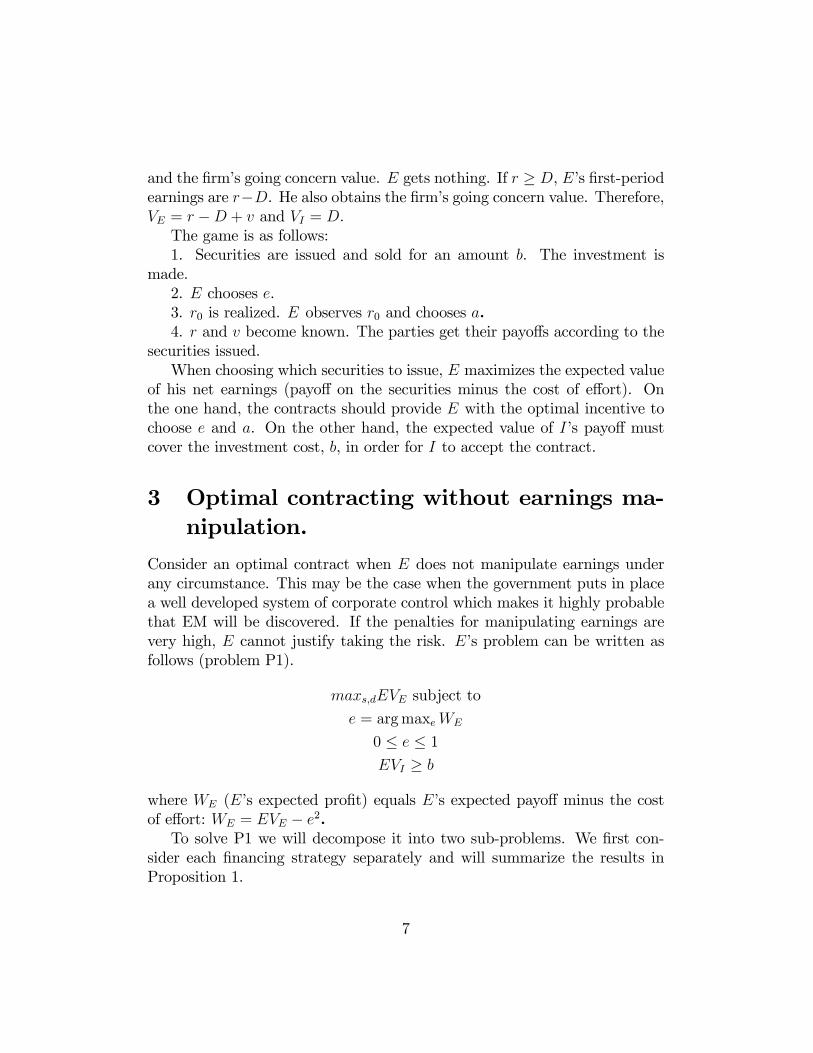
and the �rm�s going concern value. E gets nothing. If r � D, E�s �rst-periodearnings are r�D. He also obtains the �rm�s going concern value. Therefore,VE = r �D + v and VI = D.The game is as follows:1. Securities are issued and sold for an amount b. The investment is

made.2. E chooses e.3. r0 is realized. E observes r0 and chooses a.4. r and v become known. The parties get their payo¤s according to the

securities issued.When choosing which securities to issue, E maximizes the expected value

of his net earnings (payo¤ on the securities minus the cost of e¤ort). Onthe one hand, the contracts should provide E with the optimal incentive tochoose e and a. On the other hand, the expected value of I�s payo¤ mustcover the investment cost, b, in order for I to accept the contract.

3 Optimal contracting without earnings ma-nipulation.

Consider an optimal contract when E does not manipulate earnings underany circumstance. This may be the case when the government puts in placea well developed system of corporate control which makes it highly probablethat EM will be discovered. If the penalties for manipulating earnings arevery high, E cannot justify taking the risk. E�s problem can be written asfollows (problem P1).

maxs;dEVE subject to

e = argmaxeWE

0 � e � 1EVI � b

where WE (E�s expected pro�t) equals E�s expected payo¤ minus the costof e¤ort: WE = EVE � e2.To solve P1 we will decompose it into two sub-problems. We �rst con-

sider each �nancing strategy separately and will summarize the results inProposition 1.

7

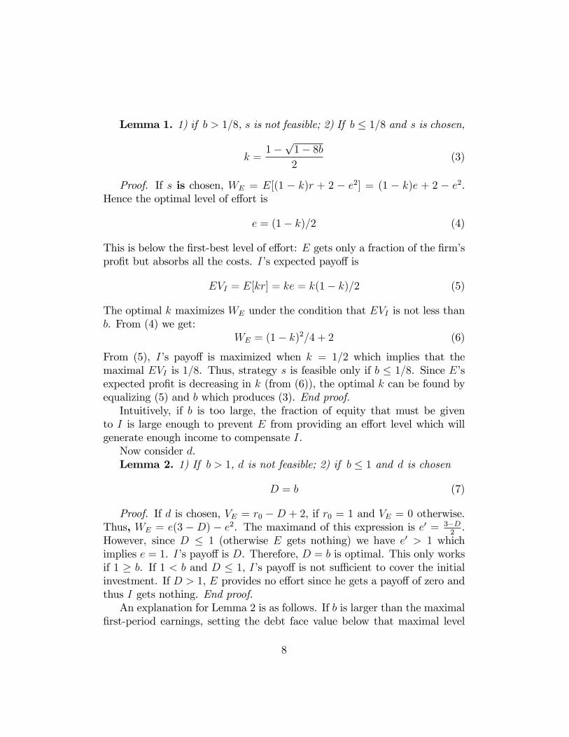
Lemma 1. 1) if b > 1=8, s is not feasible; 2) If b � 1=8 and s is chosen,

k =1�

p1� 8b2

(3)

Proof. If s is chosen, WE = E[(1 � k)r + 2 � e2] = (1 � k)e + 2 � e2.Hence the optimal level of e¤ort is

e = (1� k)=2 (4)

This is below the �rst-best level of e¤ort: E gets only a fraction of the �rm�spro�t but absorbs all the costs. I�s expected payo¤ is

EVI = E[kr] = ke = k(1� k)=2 (5)

The optimal k maximizes WE under the condition that EVI is not less thanb. From (4) we get:

WE = (1� k)2=4 + 2 (6)

From (5), I�s payo¤ is maximized when k = 1=2 which implies that themaximal EVI is 1=8. Thus, strategy s is feasible only if b � 1=8. Since E�sexpected pro�t is decreasing in k (from (6)), the optimal k can be found byequalizing (5) and b which produces (3). End proof.Intuitively, if b is too large, the fraction of equity that must be given

to I is large enough to prevent E from providing an e¤ort level which willgenerate enough income to compensate I.Now consider d.Lemma 2. 1) If b > 1, d is not feasible; 2) if b � 1 and d is chosen

D = b (7)

Proof. If d is chosen, VE = r0 �D + 2, if r0 = 1 and VE = 0 otherwise.Thus, WE = e(3 � D) � e2. The maximand of this expression is e0 = 3�D

2.

However, since D � 1 (otherwise E gets nothing) we have e0 > 1 whichimplies e = 1. I�s payo¤ is D. Therefore, D = b is optimal. This only worksif 1 � b. If 1 < b and D � 1, I�s payo¤ is not su¢ cient to cover the initialinvestment. If D > 1, E provides no e¤ort since he gets a payo¤ of zero andthus I gets nothing. End proof.An explanation for Lemma 2 is as follows. If b is larger than the maximal

�rst-period earnings, setting the debt face value below that maximal level

8

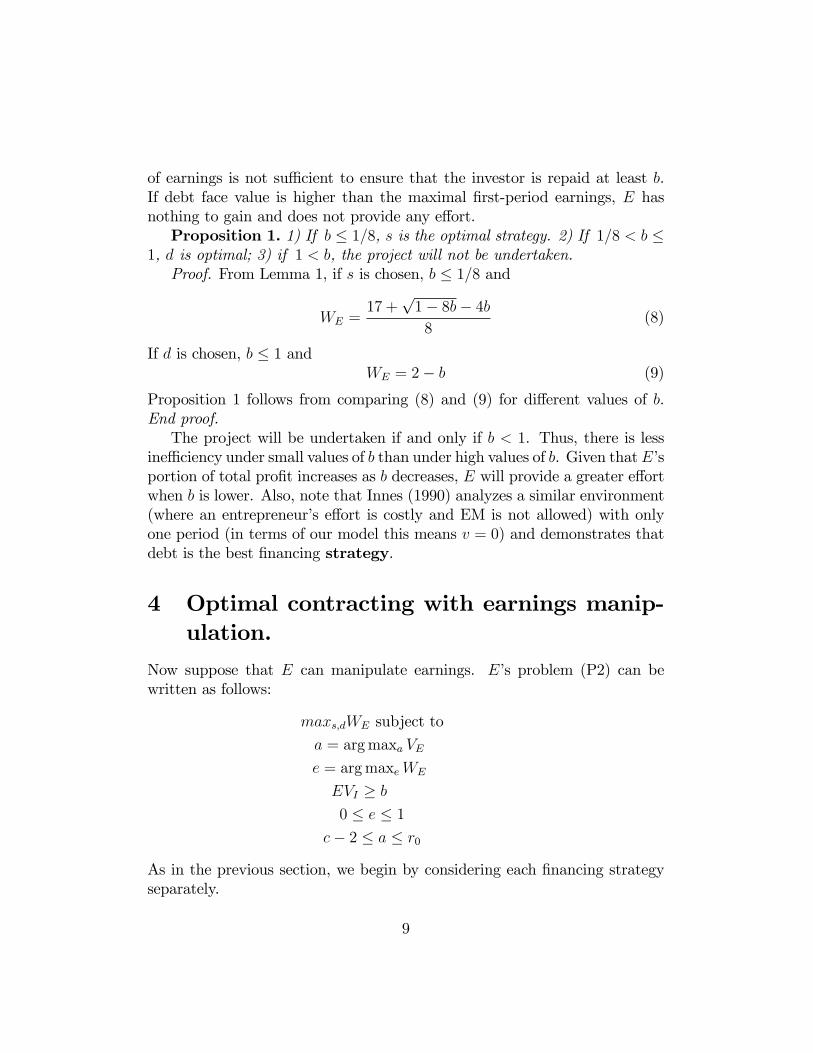
of earnings is not su¢ cient to ensure that the investor is repaid at least b.If debt face value is higher than the maximal �rst-period earnings, E hasnothing to gain and does not provide any e¤ort.Proposition 1. 1) If b � 1=8, s is the optimal strategy. 2) If 1=8 < b �

1, d is optimal; 3) if 1 < b, the project will not be undertaken.Proof. From Lemma 1, if s is chosen, b � 1=8 and

WE =17 +

p1� 8b� 4b8

(8)

If d is chosen, b � 1 andWE = 2� b (9)

Proposition 1 follows from comparing (8) and (9) for di¤erent values of b.End proof.The project will be undertaken if and only if b < 1. Thus, there is less

ine¢ ciency under small values of b than under high values of b. Given thatE�sportion of total pro�t increases as b decreases, E will provide a greater e¤ortwhen b is lower. Also, note that Innes (1990) analyzes a similar environment(where an entrepreneur�s e¤ort is costly and EM is not allowed) with onlyone period (in terms of our model this means v = 0) and demonstrates thatdebt is the best �nancing strategy.

4 Optimal contracting with earnings manip-ulation.

Now suppose that E can manipulate earnings. E�s problem (P2) can bewritten as follows:

maxs;dWE subject to

a = argmaxa VE

e = argmaxeWE

EVI � b0 � e � 1

c� 2 � a � r0

As in the previous section, we begin by considering each �nancing strategyseparately.

9

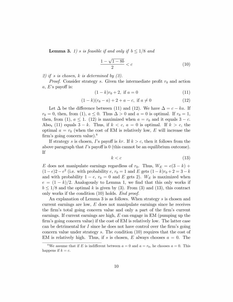
Lemma 3. 1) s is feasible if and only if b � 1=8 and

1�p1� 8b2

< c (10)

2) if s is chosen, k is determined by (3).Proof. Consider strategy s. Given the intermediate pro�t r0 and action

a, E�s payo¤ is:(1� k)r0 + 2; if a = 0 (11)

(1� k)(r0 � a) + 2 + a� c; if a 6= 0 (12)

Let � be the di¤erence between (11) and (12). We have � = c � ka. Ifr0 = 0, then, from (1), a � 0. Thus � > 0 and a = 0 is optimal. If r0 = 1,then, from (1), a � 1. (12) is maximized when a = r0 and it equals 3 � c.Also, (11) equals 3 � k. Thus, if k < c, a = 0 is optimal. If k > c, theoptimal a = r0 (when the cost of EM is relatively low, E will increase the�rm�s going concern value).8

If strategy s is chosen, I�s payo¤ is kr. If k > c, then it follows from theabove paragraph that I�s payo¤ is 0 (this cannot be an equilibrium outcome).If

k < c (13)

E does not manipulate earnings regardless of r0. Thus, WE = e(3 � k) +(1� e)2� e2 (i.e. with probability e, r0 = 1 and E gets (1� k)r0+2 = 3� kand with probability 1 � e, r0 = 0 and E gets 2). WE is maximized whene = (1 � k)=2. Analogously to Lemma 1, we �nd that this only works ifb � 1=8 and the optimal k is given by (3). From (3) and (13), this contractonly works if the condition (10) holds. End proof.An explanation of Lemma 3 is as follows. When strategy s is chosen and

current earnings are low, E does not manipulate earnings since he receivesthe �rm�s total going concern value and only a part of the �rm�s currentearnings. If current earnings are high, E can engage in EM (pumping up the�rm�s going concern value) if the cost of EM is relatively low. The latter casecan be detrimental for I since he does not have control over the �rm�s goingconcern value under strategy s. The condition (10) requires that the cost ofEM is relatively high. Thus, if s is chosen, E always chooses a = 0. The

8We assume that if E is indi¤erent between a = 0 and a = r0, he chooses a = 0. Thishappens if k = c.

10

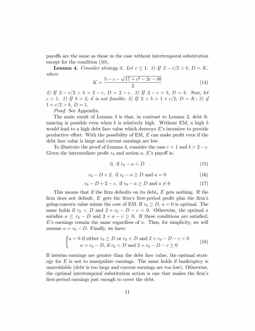
payo¤s are the same as those in the case without intertemporal substitutionexcept for the condition (10).Lemma 4. Consider strategy d. Let c � 1. 1) If 2 � c=2 < b, D = K,

where

K =5� c�

p17 + c2 � 2c� 8b2

(14)

2) If 2 � c=2 > b > 2 � c, D = 2 � c. 3) If 2 � c > b, D = b. Now, letc > 1. 1) If b > 2, d is not feasible; 2) If 2 > b > 1 + c=2, D = K; 3) if1 + c=2 > b, D = 1.Proof. See Appendix.The main result of Lemma 4 is that, in contrast to Lemma 2, debt �-

nancing is possible even when b is relatively high. Without EM, a high bwould lead to a high debt face value which destroys E�s incentive to provideproductive e¤ort. With the possibility of EM, E can make pro�t even if thedebt face value is large and current earnings are low.To illustrate the proof of Lemma 4, consider the case c < 1 and b > 2� c.

Given the intermediate pro�t r0 and action a, E�s payo¤ is:

0; if r0 � a < D (15)

r0 �D + 2; if r0 � a � D and a = 0 (16)

r0 �D + 2� c; if r0 � a � D and a 6= 0 (17)

This means that if the �rm defaults on its debt, E gets nothing. If the�rm does not default, E gets the �rm�s �rst-period pro�t plus the �rm�sgoing-concern value minus the cost of EM. If r0 � D, a = 0 is optimal. Thesame holds if r0 < D and 2 + r0 � D � c < 0. Otherwise, the optimal asatis�es a � r0 � D and 2 + a � c � 0. If these conditions are satis�ed,E�s earnings remain the same regardless of a. Thus, for simplicity, we willassume a = r0 �D. Finally, we have:�

a = 0 if either r0 � D or r0 < D and 2 + r0 �D � c < 0a = r0 �D, if r0 < D and 2 + r0 �D � c � 0

(18)

If interim earnings are greater than the debt face value, the optimal strat-egy for E is not to manipulate earnings. The same holds if bankruptcy isunavoidable (debt is too large and current earnings are too low). Otherwise,the optimal intertemporal substitution action is one that makes the �rm�s�rst-period earnings just enough to cover the debt.

11

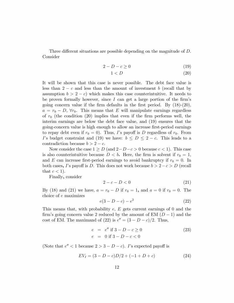
Three di¤erent situations are possible depending on the magnitude of D.Consider

2�D � c � 0 (19)

1 < D (20)

It will be shown that this case is never possible. The debt face value isless than 2 � c and less than the amount of investment b (recall that byassumption b > 2 � c) which makes this case counterintuitive. It needs tobe proven formally however, since I can get a large portion of the �rm�sgoing concern value if the �rm defaults in the �rst period. By (18)-(20),a = r0 � D, 8r0. This means that E will manipulate earnings regardlessof r0 (the condition (20) implies that even if the �rm performs well, theinterim earnings are below the debt face value, and (19) ensures that thegoing-concern value is high enough to allow an increase �rst-period earningsto repay debt even if r0 = 0). Thus, I�s payo¤ is D regardless of r0. FromI�s budget constraint and (19) we have: b � D � 2 � c. This leads to acontradiction because b > 2� c.Now consider the case 1 � D (and 2�D�c > 0 because c < 1). This case

is also counterintuitive because D < b. Here, the �rm is solvent if r0 = 1,and E can increase �rst-period earnings to avoid bankruptcy if r0 = 0. Inboth cases, I�s payo¤ is D. This does not work because b > 2� c > D (recallthat c < 1).Finally, consider

2� c�D < 0 (21)

By (18) and (21) we have, a = r0 � D if r0 = 1, and a = 0 if r0 = 0. Thechoice of e maximizes

e(3�D � c)� e2 (22)

This means that, with probability e, E gets current earnings of 0 and the�rm�s going concern value 2 reduced by the amount of EM (D � 1) and thecost of EM. The maximand of (22) is e00 = (3�D � c)=2. Thus,

e = e00 if 3�D � c � 0 (23)

e = 0 if 3�D � c < 0

(Note that e00 < 1 because 2 > 3�D � c). I�s expected payo¤ is

EVI = (3�D � c)D=2 + (�1 +D + c) (24)

12

This means that debtholders receive D (when r0 = 1) with probability e00

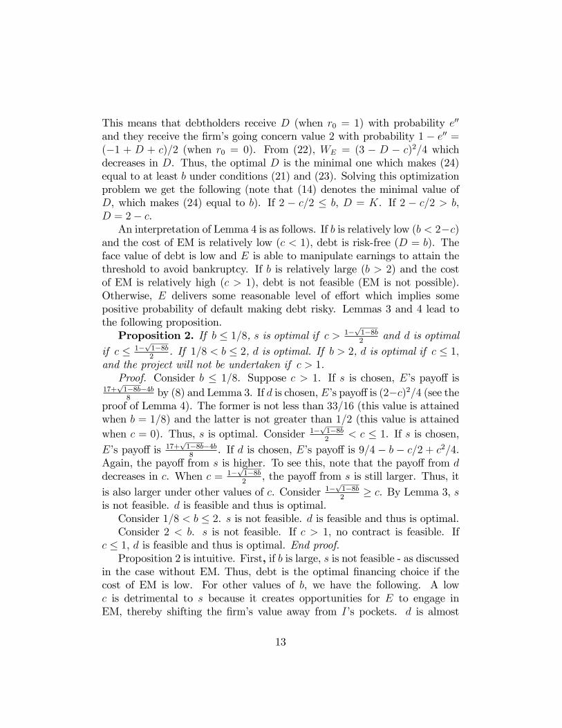
and they receive the �rm�s going concern value 2 with probability 1 � e00 =(�1 + D + c)=2 (when r0 = 0). From (22), WE = (3 � D � c)2=4 whichdecreases in D. Thus, the optimal D is the minimal one which makes (24)equal to at least b under conditions (21) and (23). Solving this optimizationproblem we get the following (note that (14) denotes the minimal value ofD, which makes (24) equal to b). If 2 � c=2 � b, D = K. If 2 � c=2 > b,D = 2� c.An interpretation of Lemma 4 is as follows. If b is relatively low (b < 2�c)

and the cost of EM is relatively low (c < 1), debt is risk-free (D = b). Theface value of debt is low and E is able to manipulate earnings to attain thethreshold to avoid bankruptcy. If b is relatively large (b > 2) and the costof EM is relatively high (c > 1), debt is not feasible (EM is not possible).Otherwise, E delivers some reasonable level of e¤ort which implies somepositive probability of default making debt risky. Lemmas 3 and 4 lead tothe following proposition.Proposition 2. If b � 1=8, s is optimal if c > 1�

p1�8b2

and d is optimal

if c � 1�p1�8b2

. If 1=8 < b � 2, d is optimal. If b > 2, d is optimal if c � 1;and the project will not be undertaken if c > 1.Proof. Consider b � 1=8. Suppose c > 1. If s is chosen, E�s payo¤ is

17+p1�8b�4b8

by (8) and Lemma 3. If d is chosen, E�s payo¤is (2�c)2=4 (see theproof of Lemma 4). The former is not less than 33=16 (this value is attainedwhen b = 1=8) and the latter is not greater than 1=2 (this value is attainedwhen c = 0). Thus, s is optimal. Consider 1�

p1�8b2

< c � 1. If s is chosen,E�s payo¤ is 17+

p1�8b�4b8

. If d is chosen, E�s payo¤ is 9=4 � b � c=2 + c2=4.Again, the payo¤ from s is higher. To see this, note that the payo¤ from ddecreases in c. When c = 1�

p1�8b2

, the payo¤ from s is still larger. Thus, it

is also larger under other values of c. Consider 1�p1�8b2

� c. By Lemma 3, sis not feasible. d is feasible and thus is optimal.Consider 1=8 < b � 2. s is not feasible. d is feasible and thus is optimal.Consider 2 < b. s is not feasible. If c > 1, no contract is feasible. If

c � 1, d is feasible and thus is optimal. End proof.Proposition 2 is intuitive. First, if b is large, s is not feasible - as discussed

in the case without EM. Thus, debt is the optimal �nancing choice if thecost of EM is low. For other values of b, we have the following. A lowc is detrimental to s because it creates opportunities for E to engage inEM, thereby shifting the �rm�s value away from I�s pockets. d is almost

13

always accompanied by EM, so reducing the cost of EM is bene�cial for debt�nancing.Corollary 1 considers the e¤ect of changes in b on the optimal choice

of contract. It is shown that when c is relatively small, �rms with a highb issue debt while �rms with the same c but a low b issue equity. If b isrelatively small, E will �nance the project by issuing stock. The �rm�s goingconcern value will fully cover the investor�s investment. The entrepreneurwill keep 100% of current period earnings which will mitigate the moralhazard problem. If b is large, then �nancing in this way may not be feasible.Therefore, debt becomes optimal.Corollary 1. If 1�

p1�8b2

� c, d is optimal. If 1�p1�8b2

< c � 1, s isoptimal if b � 1=8, and d is optimal if b > 1=8. If c > 1, s is optimal ifb � 1=8, d is optimal if 1=8 < b � 2, and no contract is feasible if b > 2.Proof. Follows directly from Proposition 2.Corollary 2. Earnings manipulation can appear in equilibrium. Earn-

ings manipulation is more probable as c decreases and b increases.Proof. From Proposition 2, if, for instance, c < 1 and b > 2� c, the equi-

librium outcome is �nancing by debt and, if r0 = 1, the �rm will manipulateearnings. Also, from Proposition 2, for a given b, debt �nancing is optimalwhen c is relatively low. In most cases, debt �nancing, in contrast to equity�nancing, will be accompanied by earnings manipulation (see the proof ofLemma 4). From Corollary 1, the same holds for high values of b. End proof.

5 Can earnings manipulation enhance a �rm�svalue?

We now compare �rms that are involved in EM (Section 4) with those thatare not (Section 3). If the amount of investment is large (b > 1), a �rmthat does not manipulate earnings will not undertake projects with positivevalue. In contrast, a �rm that manipulates earnings will undertake the sameprojects. If the amount of investment is low and EM is not possible, �nancingwith equity is optimal. If a �rm can manipulate earnings, equity may stillbe optimal. However, for equity to be optimal, the cost of EM must be high- otherwise the entrepreneur will "convert" current earnings into ine¢ cientlong-term projects making the issuance of equity unfeasible (ex-ante). In thelatter case, debt becomes optimal. This will usually be accompanied by EM:

14

the entrepreneur will try to achieve the threshold to avoid bankruptcy. Itfollows that there is a trade-o¤ in social e¢ ciency between the bene�ts fromEM improving the entrepreneur�s e¤ort and the costs of EM.Proposition 3. If 1 < b � 2, �rms that manipulate earnings have a

higher value than �rms that do not :Otherwise, �rms that manipulate earningshave a higher value if and only if the cost of manipulation is low.Proof. Let VEM denote the value of �rms that can manipulate earnings

and let VN denote the value of �rms that cannot manipulate earnings. Asfollows from Proposition 1, if b > 1 and earnings manipulation is not allowed,the �rm does not invest and thus VN = 0. According to Proposition 2, if1 < b � 2 or if b > 2 and c < 1, �rms that can engage in EM will usedebt �nancing and invest in the project. The value of these �rms will bepositive. Consider 1=8 < b � 1. According to Proposition 1, VN = 2� b. Ifc � 1, VEM = 9=4 � b � c=2 + c2=4 (from the proof of Proposition 2). Thisexpression decreases in c when c � 1. The minimal value, 2� b, is attainedwhen c = 1. Therefore, the value of �rms that can engage in EM is greaterthan or equal to the value of �rms that are not involved in EM. If c > 1,VEM = (2 � c)2=4. This is less than 2 � b. Therefore, �rms that do notmanipulate earnings have a higher value. If 1=8 � b, VN = 17+

p1�8b�4b8

. If

c > 1�p1�8b2

, �rms that manipulate earnings have the same value as �rms that

do not. If c � 1�p1�8b2

, VEM = 9=4�b�c=2+c2=4. Consider � = VEM�VN .This expression decreases in c. When c = 0, � > 0. When c = 1�

p1�8b2

,� < 0. The proposition follows from the continuity of � in c. End proof.

6 Model discussion.

1. Suppose that it is possible to write an enforceable contract contingent onthe �rm�s total value. Then, for any contract found in section 4, there existsan alternative contract contingent on the �rm�s total value that will provideE with a higher payo¤. To illustrate this, consider c < 1 and b < 2 � c.If a �rm can engage in EM, the optimal contract is analogous to the onedescribed in proposition 2. E�s e¤ort is e = 1=2 and the parties expectedpayo¤s are:

WE = 9=4� b� c (25)

and EVI = b. D = b is optimal. E manipulates earnings regardless of r0.When r0 = 0 he receives 2 � b � c and when r0 = 1 he receives 3 � b � c.

15

Now suppose the parties write a contract where E gets 2 � b if the �rm�stotal value is 2 or less and 3 � b if the �rm�s total value is greater than 2.The optimal e¤ort maximizes e(3 � b) + (1 � e)(2 � b) � e2. e = 1=2 isoptimal. Also, a = 0 because any a > 0 will only reduce the �rm�s totalvalue. E�s expected payo¤ is 9=4 � b which is greater than (25). EVI =1=2(3� (3� b)) + 1=2(2� (2� b)) = b. Therefore, we have a better contractwhich does not involve EM.2. Now suppose that the model does not contain productive e¤ort. In

this case, equity is the optimal �nancing contract since it eliminates theintertemporal substitution problem (this idea is developed in Jensen, 2003).Other securities will be useless. This scenario is not realistic since �rms donot issue equity alone.3. Suppose that the �rm can issue convertible debt. This is similar to

standard debt described in the model except that I can purchase a fraction ofthe �rm�s shares when it is solvent. However, since E remains in control, hewill cream-o¤ the �rm�s going concern value. Hence, the modelling is similarto standard debt.4. Long-term debt is not considered (in the spirit of incomplete contract

literature) because it cannot be enforced. Since the creditors do not haveproperty rights on the remaining assets, the owners will capture the �rm�sentire going-concern value.5. One can make additional assumptions about the �rst and second pe-

riod sharing rules based on a continuous earnings distribution function ordi¤erent control shifting scenarios. These scenarios may yield some new re-sults. For instance, one can assume that E also has some private bene�tsfrom controlling the �rm. However, the main idea that EM can improveproductive e¤ort will not be a¤ected.

7 Implications.

1. We have shown that EM can be a part of the equilibrium relationshipbetween �rms�insiders and outsiders. This holds even if the cost of EM isrelatively high (as follows from Proposition 2). Investors accept some degreeof EM because this increases the insiders�incentive to provide a high levelproductive e¤ort.2. From Proposition 3, if the cost of EM is relatively low, EM can be

socially e¢ cient. EM can enhance a �rm�s value when compared to the case

16

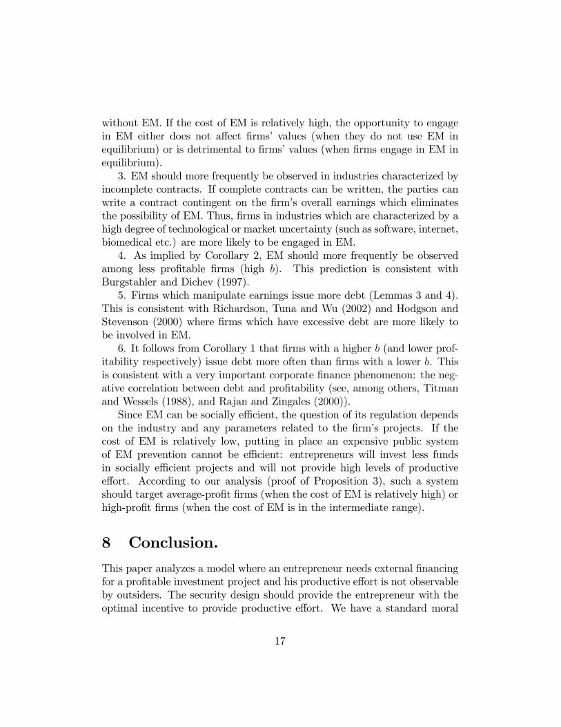
without EM. If the cost of EM is relatively high, the opportunity to engagein EM either does not a¤ect �rms� values (when they do not use EM inequilibrium) or is detrimental to �rms�values (when �rms engage in EM inequilibrium).3. EM should more frequently be observed in industries characterized by

incomplete contracts. If complete contracts can be written, the parties canwrite a contract contingent on the �rm�s overall earnings which eliminatesthe possibility of EM. Thus, �rms in industries which are characterized by ahigh degree of technological or market uncertainty (such as software, internet,biomedical etc.) are more likely to be engaged in EM.4. As implied by Corollary 2, EM should more frequently be observed

among less pro�table �rms (high b). This prediction is consistent withBurgstahler and Dichev (1997).5. Firms which manipulate earnings issue more debt (Lemmas 3 and 4).

This is consistent with Richardson, Tuna and Wu (2002) and Hodgson andStevenson (2000) where �rms which have excessive debt are more likely tobe involved in EM.6. It follows from Corollary 1 that �rms with a higher b (and lower prof-

itability respectively) issue debt more often than �rms with a lower b. Thisis consistent with a very important corporate �nance phenomenon: the neg-ative correlation between debt and pro�tability (see, among others, Titmanand Wessels (1988), and Rajan and Zingales (2000)).Since EM can be socially e¢ cient, the question of its regulation depends

on the industry and any parameters related to the �rm�s projects. If thecost of EM is relatively low, putting in place an expensive public systemof EM prevention cannot be e¢ cient: entrepreneurs will invest less fundsin socially e¢ cient projects and will not provide high levels of productivee¤ort. According to our analysis (proof of Proposition 3), such a systemshould target average-pro�t �rms (when the cost of EM is relatively high) orhigh-pro�t �rms (when the cost of EM is in the intermediate range).

8 Conclusion.

This paper analyzes a model where an entrepreneur needs external �nancingfor a pro�table investment project and his productive e¤ort is not observableby outsiders. The security design should provide the entrepreneur with theoptimal incentive to provide productive e¤ort. We have a standard moral

17

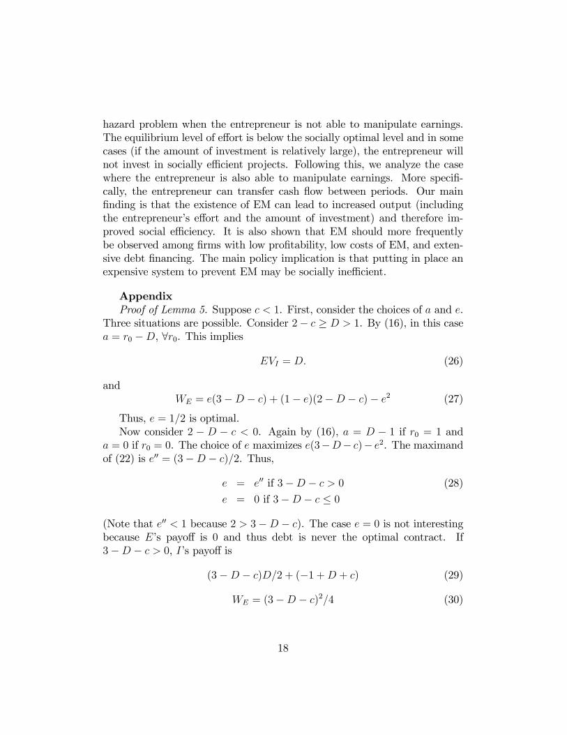
hazard problem when the entrepreneur is not able to manipulate earnings.The equilibrium level of e¤ort is below the socially optimal level and in somecases (if the amount of investment is relatively large), the entrepreneur willnot invest in socially e¢ cient projects. Following this, we analyze the casewhere the entrepreneur is also able to manipulate earnings. More speci�-cally, the entrepreneur can transfer cash �ow between periods. Our main�nding is that the existence of EM can lead to increased output (includingthe entrepreneur�s e¤ort and the amount of investment) and therefore im-proved social e¢ ciency. It is also shown that EM should more frequentlybe observed among �rms with low pro�tability, low costs of EM, and exten-sive debt �nancing. The main policy implication is that putting in place anexpensive system to prevent EM may be socially ine¢ cient.

AppendixProof of Lemma 5. Suppose c < 1. First, consider the choices of a and e.

Three situations are possible. Consider 2� c � D > 1. By (16), in this casea = r0 �D, 8r0. This implies

EVI = D: (26)

andWE = e(3�D � c) + (1� e)(2�D � c)� e2 (27)

Thus, e = 1=2 is optimal.Now consider 2 � D � c < 0. Again by (16), a = D � 1 if r0 = 1 and

a = 0 if r0 = 0. The choice of e maximizes e(3�D� c)� e2. The maximandof (22) is e00 = (3�D � c)=2. Thus,

e = e00 if 3�D � c > 0 (28)

e = 0 if 3�D � c � 0

(Note that e00 < 1 because 2 > 3�D � c). The case e = 0 is not interestingbecause E�s payo¤ is 0 and thus debt is never the optimal contract. If3�D � c > 0, I�s payo¤ is

(3�D � c)D=2 + (�1 +D + c) (29)

WE = (3�D � c)2=4 (30)

18

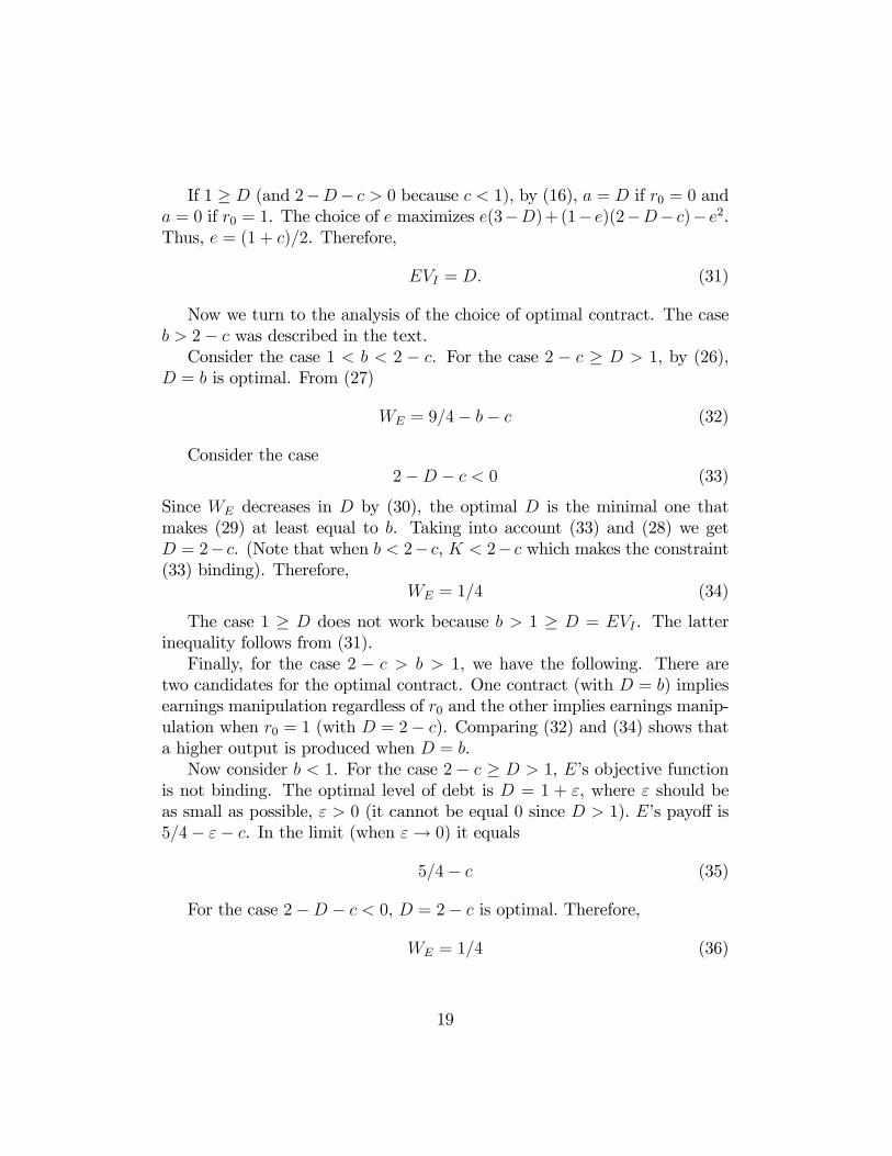
If 1 � D (and 2�D� c > 0 because c < 1), by (16), a = D if r0 = 0 anda = 0 if r0 = 1. The choice of e maximizes e(3�D)+ (1� e)(2�D� c)� e2.Thus, e = (1 + c)=2. Therefore,

EVI = D: (31)

Now we turn to the analysis of the choice of optimal contract. The caseb > 2� c was described in the text.Consider the case 1 < b < 2 � c. For the case 2 � c � D > 1, by (26),

D = b is optimal. From (27)

WE = 9=4� b� c (32)

Consider the case2�D � c < 0 (33)

Since WE decreases in D by (30), the optimal D is the minimal one thatmakes (29) at least equal to b. Taking into account (33) and (28) we getD = 2� c. (Note that when b < 2� c, K < 2� c which makes the constraint(33) binding). Therefore,

WE = 1=4 (34)

The case 1 � D does not work because b > 1 � D = EVI . The latterinequality follows from (31).Finally, for the case 2 � c > b > 1, we have the following. There are

two candidates for the optimal contract. One contract (with D = b) impliesearnings manipulation regardless of r0 and the other implies earnings manip-ulation when r0 = 1 (with D = 2� c). Comparing (32) and (34) shows thata higher output is produced when D = b.Now consider b < 1. For the case 2 � c � D > 1, E�s objective function

is not binding. The optimal level of debt is D = 1 + ", where " should beas small as possible, " > 0 (it cannot be equal 0 since D > 1). E�s payo¤ is5=4� "� c. In the limit (when "! 0) it equals

5=4� c (35)

For the case 2�D � c < 0, D = 2� c is optimal. Therefore,

WE = 1=4 (36)

19

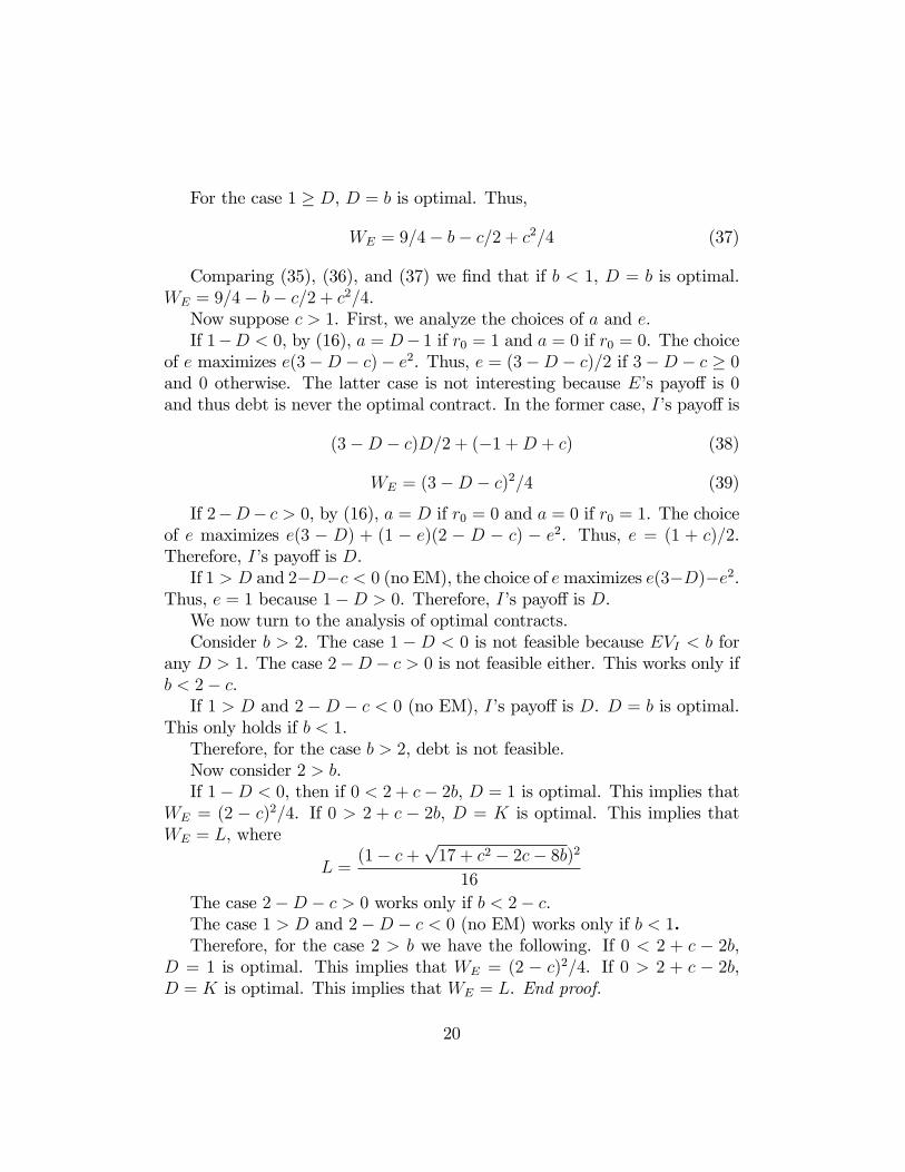
For the case 1 � D, D = b is optimal. Thus,

WE = 9=4� b� c=2 + c2=4 (37)

Comparing (35), (36), and (37) we �nd that if b < 1, D = b is optimal.WE = 9=4� b� c=2 + c2=4.Now suppose c > 1. First, we analyze the choices of a and e.If 1�D < 0, by (16), a = D� 1 if r0 = 1 and a = 0 if r0 = 0. The choice

of e maximizes e(3�D � c)� e2. Thus, e = (3�D � c)=2 if 3�D � c � 0and 0 otherwise. The latter case is not interesting because E�s payo¤ is 0and thus debt is never the optimal contract. In the former case, I�s payo¤ is

(3�D � c)D=2 + (�1 +D + c) (38)

WE = (3�D � c)2=4 (39)

If 2�D� c > 0, by (16), a = D if r0 = 0 and a = 0 if r0 = 1. The choiceof e maximizes e(3 � D) + (1 � e)(2 � D � c) � e2. Thus, e = (1 + c)=2.Therefore, I�s payo¤ is D.If 1 > D and 2�D�c < 0 (no EM), the choice of emaximizes e(3�D)�e2.

Thus, e = 1 because 1�D > 0. Therefore, I�s payo¤ is D.We now turn to the analysis of optimal contracts.Consider b > 2. The case 1 �D < 0 is not feasible because EVI < b for

any D > 1. The case 2�D� c > 0 is not feasible either. This works only ifb < 2� c.If 1 > D and 2�D � c < 0 (no EM), I�s payo¤ is D. D = b is optimal.

This only holds if b < 1.Therefore, for the case b > 2, debt is not feasible.Now consider 2 > b.If 1�D < 0, then if 0 < 2 + c� 2b, D = 1 is optimal. This implies that

WE = (2 � c)2=4. If 0 > 2 + c � 2b, D = K is optimal. This implies thatWE = L, where

L =(1� c+

p17 + c2 � 2c� 8b)216

The case 2�D � c > 0 works only if b < 2� c.The case 1 > D and 2�D � c < 0 (no EM) works only if b < 1.Therefore, for the case 2 > b we have the following. If 0 < 2 + c � 2b,

D = 1 is optimal. This implies that WE = (2 � c)2=4. If 0 > 2 + c � 2b,D = K is optimal. This implies that WE = L. End proof.

20

References

[1] Burgstahler, D. and I. Dichev. 1997. Earnings Management to AvoidEarnings Decreases and Losses. Journal of Accounting and Economics24 (1), 1-33.

[2] Cornelli, F. and O. Yosha. 2003. Stage Financing and the Role of Con-vertible Securities. Review of Economic Studies 70, 1-32.

[3] Crocker, K., and J. Slemord. 2005. The Economics of Earnings Manip-ulation and Managerial Compensation. Working paper.

[4] Dechow, P., Sloan, R., and A. Sweeney. 1996. Causes and Consequencesof Earnings Manipulation: An Analysis of Firms Subject to EnforcementActions by SEC. Contemporary Accounting Research 13, 1-36.

[5] Degeorge, F., Patel, J. and R. Zeckhauser. 1999. Earnings Managementto Exceed Thresholds. The Journal of Business 72 (1), 1-33.

[6] Erickson M., M. Hanlon and E. Maydew. 2003. Is There a Link BetweenExecutive Compensation and Accounting Fraud? Working paper, Uni-versity of Michigan

[7] Hart, O. 1995. Firms, Contracts and Financial Structure. Oxford Uni-versity Press.

[8] Hodgson, A. and P. Stevenson-Clarke. Accounting Variables and StockReturns: The Impact of Leverage. As published in Paci�c AccountingReview, December 2000.

[9] Innes, R., 1990. Limited Liability and Incentive Contracting with ex-ante Choices. Journal of Economic Theory 52, 45-67.

[10] Jensen, M. 2003. Paying People to Lie: the Truth about the BudgetingProcess. Europen Financial Management 9 (3), 379-406.

[11] Johnson, G., and E. Talley. 2005. Corporate Governance, ExecutiveCompensation and Securities Litigation. SSRN Working paper.

[12] Kaplan, S., and P. Stromberg, P. 2003. Financial Contracting TheoryMeets the Real World: An Empirical Analysis of Venture Capital Con-tracts. The Review of Economic Studies 70, 281-316.

21

[13] Rajan, R. G., and L. Zingales. 1995. What do we know about CapitalStructure? Some Evidence from International Data. Journal of Finance50, 1421-1460.

[14] Richardson, S., A. Tuna, and M. Wu. Predicting Earnings Management:The Case of Earnings Restatements SSRN working paper.

[15] Roychowdhury, S. Earnings Management through Real Activities Ma-nipulation. Massachusetts Institute of Technology, 2006. Working PaperSeries

[16] Titman, S., and R. Wessels. 1988. The Determinants of Capital Struc-ture Choice. Journal of Finance 43, 1-19.

[17] Yu Q., B. Du and Q. Sun. 2004. Earnings Management at Thresholds:Evidence from Rights Issues in China. Working paper, Nanyang BusinessSchool.

22