CAN Eye-diagram Mask Testing Application Note Eye-diagram mask testing is used in a broad range of today’s serial bus applications. An eye-diagram is basically an infinite persisted overlay of all bits captured by an oscilloscope to show when bits are valid. This provides a composite picture of the overall quality of a system’s physical layer characteristics, which includes amplitude variations, timing uncertainties, and infrequent signal anomalies. Eye-diagram testing can be performed on differential Controller Area Network (CAN) signals using an Agilent 3000 X-Series oscilloscope licensed with the DSOX3AUTO trigger and decode option (CAN & LIN), along with the DSOX3MASK mask test option. Various CAN mask files can be downloaded from Agilent’s website at no charge. Save the appropriate CAN eye-diagram mask files (based on baud rate, probing polarity, and network length) to your personal USB memory device. The following CAN mask files are available: Introduction • CAN-diff (H-L) 125kbps-400m.msk • CAN-diff (L-H) 125kbps-400m.msk • CAN-diff (H-L) 250kbps-200m.msk • CAN-diff (L-H) 250kbps-200m.msk • CAN-diff (H-L) 500kbps-80m.msk • CAN-diff (L-H) 500kbps-80m.msk • CAN-diff (H-L) 500kbps-10m.msk • CAN-diff (L-H) 500kbps-10m.msk • CAN-diff (H-L) 800kbps-40m.msk • CAN-diff (L-H) 800kbps-40m.msk • CAN-diff (H-L) 1000kbps-25m.msk • CAN-diff (L-H) 1000kbps-25m.msk Introduction…………………………………….. 1 Probing the Differential CAN Bus………. 2 Step-by-step Instructions….…………….… 3 Interpreting the Eye………………………….. 3 CAN Network Delays………………………... 5 The Pass/Fail Mask………………………….. 8 Summary…………………………………………..9 System Requirements……………………….. 9 Related Literature………………………………10 Table of Contents
Transcript
CAN Eye-diagramMask Testing
Application Note
Eye-diagram mask testing is used in a broad range of
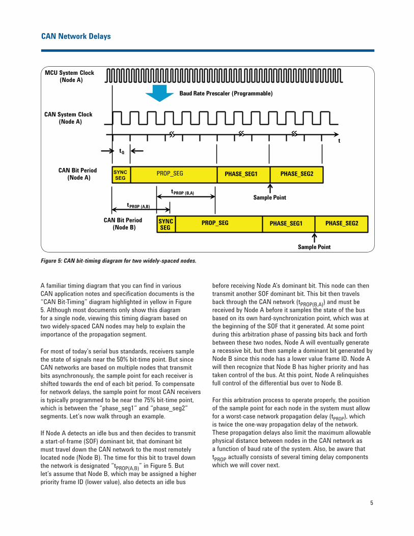
today’s serial bus applications. An eye-diagram is basically
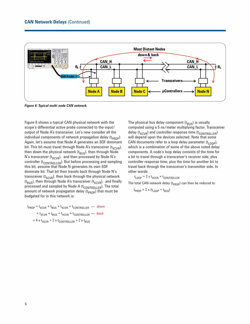
an infinite persisted overlay of all bits captured by an
oscilloscope to show when bits are valid. This provides
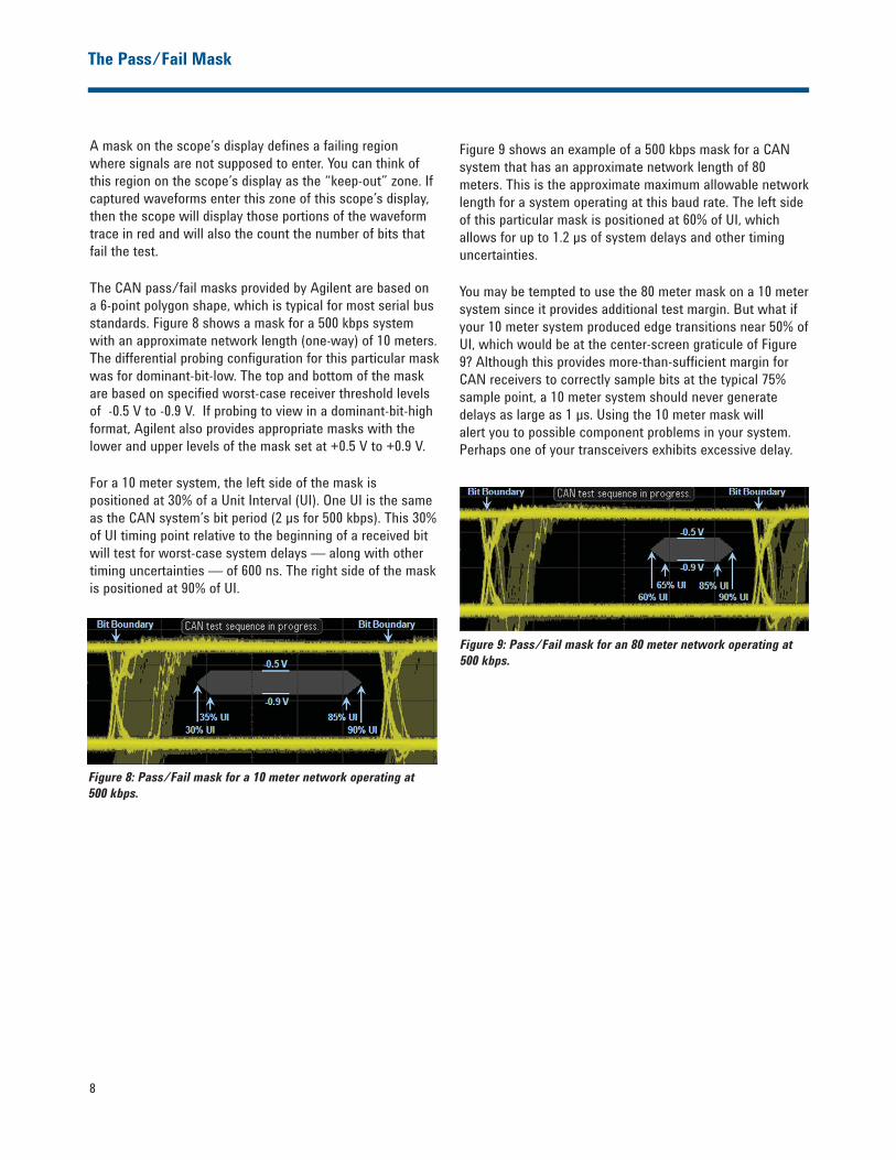
a composite picture of the overall quality of a system’s
physical layer characteristics, which includes amplitude
variations, timing uncertainties, and infrequent signal
anomalies.
Eye-diagram testing can be performed on differential
Controller Area Network (CAN) signals using an Agilent
3000 X-Series oscilloscope licensed with the DSOX3AUTO
trigger and decode option (CAN & LIN), along with the
DSOX3MASK mask test option. Various CAN mask files can
be downloaded from Agilent’s website at no charge. Save
the appropriate CAN eye-diagram mask files (based on baud
rate, probing polarity, and network length) to your personal
USB memory device. The following CAN mask files are
available:
Introduction
• CAN-diff (H-L) 125kbps-400m.msk
• CAN-diff (L-H) 125kbps-400m.msk
• CAN-diff (H-L) 250kbps-200m.msk
• CAN-diff (L-H) 250kbps-200m.msk
• CAN-diff (H-L) 500kbps-80m.msk
• CAN-diff (L-H) 500kbps-80m.msk
• CAN-diff (H-L) 500kbps-10m.msk
• CAN-diff (L-H) 500kbps-10m.msk
• CAN-diff (H-L) 800kbps-40m.msk
• CAN-diff (L-H) 800kbps-40m.msk
• CAN-diff (H-L) 1000kbps-25m.msk
• CAN-diff (L-H) 1000kbps-25m.msk
Introduction…………………………………….. 1
Probing the Differential CAN Bus………. 2
Step-by-step Instructions….…………….… 3
Interpreting the Eye………………………….. 3
CAN Network Delays………………………... 5
The Pass/Fail Mask………………………….. 8
Summary…………………………………………..9
System Requirements……………………….. 9
Related Literature………………………………10
Table of Contents
2
Probing the Differential CAN Bus
CAN eye-diagram mask testing is based on capturing and
overlaying all recessive and dominate bits on the differential
bus. The differential bus must be probed using a differential
active probe. Agilent recommends using the N2791A
25-MHz differential active probe shown in Figure 1. The
attenuation setting on the probe should be set to 10:1 (not
100:1). The output of the probe should be terminated into
the scope’s default 1-MΩ input termination.
Also available is the N2792A 200-MHz bandwidth
differential active probe (not shown). This particular probe
has sufficient bandwidth for either CAN or FlexRay (up to 10
Mbps) applications. If using the N2792A differential active
probe, this probe is designed to be terminated into the
scope’s user-selectable 50-Ω input termination.
If you need to connect to DB9-SubD connectors in your
system, Agilent also offers the CAN/FlexRay DB9 probe
head (Part number 0960-2926). This differential probe head,
which is shown in the inset photo of Figure 1, is compatible
with both the N2791A and N2792A differential active
probes, and allows you to connect easily to your CAN and/
or FlexRay differential bus.
A differential active probe allows you to view signals on
the differential CAN bus in either a dominant-bit-high or
dominant-bit-low format. And CAN eye-diagram mask
testing can be performed using either polarity of probing. To
observe signals as dominant-bit-high, connect the “+” (red)
input of the differential probe to CAN_H and the “-“ (black)
input of the probe to CAN_L. Figure 2 shows a differential
CAN waveform in the dominant-bit-high format.
To observe signals in the dominant-bit-low format, connect
the “+” (red) input of the differential probe to CAN_L and
the “-“ (black) input of the probe to CAN_H. Although
connecting the differential probe to the bus in this manner
may sound backwards and perhaps unintuitive, timing
diagrams of CAN signals are typically shown in a dominant-
bit-low format. In this format, bus idle level is always high
(recessive). Also, during transmission of CAN frames, high-
level signals (recessive bits) will always be interpreted as
“1s”, while low-level signals (dominant bits) will always
be interpreted as “0s”. Figure 3 shows a differential CAN
waveform in the dominant–bit-low format.
Figure 2: Probing the differential CAN bus to show
dominant-bit-high.
Figure 1: N2791A 25-MHz Differential Active Probe and
DB9-Probe Head.
Figure 3: Probing the differential CAN bus to show
dominant-bit-low.
3
Step-by-Step Instructions to Perform a CAN Eye-diagram Mask Test
To perform a CAN eye-diagram mask test, first turn off all
channels of the oscilloscope except for the input channel
that is connected to the CAN differential bus. If you begin
with a Default Setup, only channel-1 will be turned on.
Alternatively, you can begin with the oscilloscope already
set up and triggering on the differential CAN bus. To begin
execution of a CAN eye-diagram mask test, do the following:
1. Insert your USB memory device (with the appropriate
mask file) into the scope’s front panel USB port.
2. Press the [Save/Recall] front panel key; then press the
Recall softkey.
3. Press the Recall: XXXX softkey; then select Mask as
the type of file to recall.
4. Press the Location (or Press to go, or load from)
softkey; then navigate to the appropriate mask file
based on baud rate and probing polarity
(L-H = dominant bit low, H-L = dominant bit high).
5. Press the Press to Recall softkey (or press the entry
knob) to begin a CAN eye-diagram mask test.
When the mask file is recalled, the scope will automatically
set itself up (timebase, vertical, and trigger settings) to
display overlaid CAN bits across the center six divisions
of the scope’s display. During this special sequencing test,
timebase settings and timing cursors cannot be used. To
exit a CAN eye-diagram mask test, either turn off mask
testing or press Clear Mask in the scope’s Analyze-Mask
menu. When the test is exited, the scope will restore most
oscilloscope settings to the state they were in prior to
beginning the test.
Interpreting the Eye
The CAN eye-diagram test randomly captures and overlays
every differential bit of every CAN frame based on a
unique clock recovery algorithm that emulates worst-case
CAN receiver hard-synchronization, re-synchronization,
and sampling. Figure 4 shows a CAN eye-diagram mask
test based on a system baud rate of 500 kbps with
differential probing established to obverse the waveforms
in a dominant-bit-low format. This test basically shows if
dominate and recessive bits have settled to valid/specified
levels prior to receiver sampling, which typically occurs near
the 75% bit-time point. In other words, the CAN eye-diagram
shows what the CAN receiver “sees” by synchronizing the
scope’s acquisition and display timing to the CAN receiver’s
timing. The result is a single measurement that provides
insight into the overall signal integrity of the CAN physical
layer network to show worst-case timing and worst-case
vertical amplitude variations. Overlaid and infinitely persisted bits of the eye-diagram
are continually compared against a 6-point polygon-
shaped pass/fail mask, which is based on CAN physical
layer specifications. Although there are many factors that
determine the eye-diagram test rate, Agilent’s 3000 X-Series
oscilloscope can test approximately 10,000 bits per second
based on a CAN system operating at 500 kbps and with an
approximate bus load equal to 33%.
Figure 4: CAN eye-diagram mask test on a 500 kbps differential
bus viewed in a dominant-bit-low format.
4
Interpreting the Eye (Continued)
On the vertical axis, the eye-diagram display shows various
peak-to-peak amplitudes. Variations in signal amplitudes on
the differential CAN bus are primarily due to the following:
• System noise/interference/coupling
• Different transmitters (nodes in the system) exhibiting
unique and different output characteristics
• Attenuated amplitudes due to network lengths and