Working Paper Research by Raïsa Basselier, David de Antonio Liedo, Jana Jonckheere and Geert Langenus October 2018 No 348 Can inflation expectations in business or consumer surveys improve inflation forecasts ?
Transcript
Working Paper Researchby Raïsa Basselier, David de Antonio Liedo,
Jana Jonckheere and Geert Langenus
October 2018 No 348
Can inflation expectations in business or consumer surveys improve inflation forecasts ?
Can inflation expectations in business orconsumer surveys improve inflation
forecasts?
Raısa Basselier∗, David de Antonio Liedo†, Jana Jonckheere‡, Geert Langenus§
Abstract
In this paper we develop a new model that incorporates inflation expectationsand can be used for the structural analysis of inflation, as well as for forecasting.In this latter connection, we specifically look into the usefulness of real-time surveydata for inflation projections. We contribute to the literature in two ways. First,our model extracts the inflation trend and its cycle, which is linked to real economicactivity, by exploiting a much larger information set than typically seen in thisclass of models and without the need to resort to Bayesian techniques. The reasonis that we use variables reflecting inflation expectations from consumers and firmsunder the assumption that they are consistent with the expectations derived fromthe model. Thus, our approach represents an alternative way to shrink the modelparameters and to restrict the future evolution of the factors. Second, the inflationexpectations that we use are derived from the qualitative questions on expected pricedevelopments in both the consumer and the business surveys. This latter source,in particular, is mostly neglected in the empirical literature. Our empirical resultssuggest that overall, inflation expectations in surveys provide useful information forinflation forecasts. In particular for the most recent period, models that includesurvey expectations on prices tend to outperform similar models that do not, bothfor Belgium and the euro area. Furthermore, we find that the business survey, i.e.the survey replies by the price-setters themselves, contributes most to these forecastimprovements.
∗National Bank of Belgium, Economics and Research Department, e-mail: [email protected].†National Bank of Belgium, R&D Statistics, e-mail: [email protected].‡National Bank of Belgium, Economics and Research Department, e-mail: [email protected].§National Bank of Belgium, Economics and Research Department, e-mail: [email protected] model presented in this paper has been developed and estimated with the software JDemetra+,
which is well known for seasonal adjustment, but it also contains very efficient algorithms for the esti-mation of state-space models like the ones used here. We would like to thank Jean Palate for havingdeveloped the R interface (publicly available in GitHub) that has allowed us to specify our models in Rand estimate them in JDemetra+.
1
Contents
1 Introduction 3
2 Motivation: recent inflation projections for Belgium and the euro area 6
6 Focus on the recent period and interpretation 376.1 A change in the forecast evaluation sample . . . . . . . . . . . . . . . . . . 376.2 Businesses or consumers? . . . . . . . . . . . . . . . . . . . . . . . . . . . . 39
7 Conclusion 42
8 Annexes 47
2
1 Introduction
This paper aims to assess whether the accuracy of Belgian and euro area inflation pro-
jections can be improved by explicitly incorporating information on expected price devel-
opments, drawn from the EC consumer and business surveys, into a structural model. In
recent years, inflation has generally been remarkably low in advanced countries. Conven-
tional models have, in particular, mostly failed to predict and explain the very slow pick-up
of price growth after the great recession. The “missing inflation” puzzle has fuelled the
debate in the literature on the slope of the Phillips curve. In addition, the possibility of
changes in the trend or the persistence of inflation has been discussed. Different strands
of the literature have focused on the pass-through of costs or exchange rate movements
to final prices, as well as on the role of inflation expectations and a possible deanchoring
of those expectations. However, as shown by Mankiw et al. (2003), different measures
of inflation expectations can diverge strongly. In the empirical literature, the question of
the usefulness of inflation expectations is mostly addressed by looking at implied expecta-
tions that are derived from financial market indicators and the term structure of interest
rates, as well as at (point or range) forecasts of economist experts and, to a lesser extent,
consumers. In this connection, Carroll (2003) finds that surveys regarding forecasts by
economic experts are more informative for inflation projections than price expectations
of consumer surveys. Ang et al. (2007) show that projection models for US inflation
that include expectations of professional forecasters can outperform structural Phillips
curve models. The same is true for consumer expectations in the University of Michigan
consumer survey but the accuracy gains are smaller. Literature on qualitative inflation
expectations is somewhat scarcer. Scheufele (2011) finds that qualitative inflation ex-
pectations in the ZEW survey can improve inflation forecasts for Germany. Similarly,
Forsells and Kenny (2004) show that the qualitative data on price expectations in the EC
consumer surveys can provide a reasonably accurate predictor of actual inflation. Within
this strand of literature, research on the usefulness of qualitative information provided
by producers is not strongly represented. Yet, as suggested by Bernanke (2007), the
latter can be an even more important source of information for forecasts, as the survey
respondents are the actual price-setters. Hence, we will investigate the role of (qualita-
tive) survey information on both consumers’ and producers’ inflation expectations that
3
we take from the EC consumers and business surveys. To the best of our knowledge only
a few papers have specifically used these survey data for inflation projections. One ex-
ample is Stockhammar and Osterholm (2016) who find that the inflation expectations in
the Swedish National Institute of Economic Research’s Business Tendency Survey (that,
however, also includes consumers as respondents, in addition to firms) improve model
forecast precision for Swedish inflation in a meaningful way, in particular for the shorter
horizons. Remarkably, this is much less the case for the TNS Sifo Prospera’s inflation
survey – which is conducted on behalf of the Sveriges Riksbank – that is restricted to
businesses and does not include consumers. The Federal Reserve Bank of Atlanta on the
other hand routinely uses price expectations from its business surveys to shape its views
on future inflation developments.2
This paper contributes to the literature in multiple ways. First of all, we follow the
path traced by Coibion and Gorodnichenko (2015) and Coibion et al. (2018) and add to
the scarce literature on the role of qualitative real-time survey data on inflation forecasting.
More specifically, we incorporate information from both consumers and firms and look
into their information content for both headline and core inflation. To the best of our
knowledge, no similar exercise was ever performed for Belgium or the euro area. We also
investigate which of the two surveys offers the most added value in terms of forecasting
accuracy. Furthermore, by assuming that the survey information is consistent with the
expectations derived from our proposed model, we offer a method to impose cross-equation
restrictions on the model parameters and the future evolution of the factors.
The model used is inspired by Stella and Stock (2013) and belongs to the class of
unobserved components models (UCM). Our dataset contains up to ten variables that
range from (core and total) inflation to oil prices, the import deflator, real GDP, the
unemployment rate, the mark-up, a global sentiment indicator and two variables reflecting
inflation expectations from consumers and businesses. Fluctuations of headline and core
inflation are given by a trend and a cyclical component. The latter could co-move with
the cyclical component of real activity, which is the common factor for all variables,
providing a linkage between real and nominal economic activity. This way, our model
is larger than others belonging to the same class, with the advantage that due to the
assumed model-consistency of the survey information, we do not need to specify priors
2Please refer to: https://www.frbatlanta.org/research/inflationproject/bie
4
for the multiple parameters, as done for example in Chan et al. (2016), who use bounds
to improve estimation of the trend, or in Hasenzagl et al. (2018), who propose a model
of the same class as ours.
The remainder of the paper is organised as follows. Following a description of the
motivation and context of this paper, the data that are used in the model will be described,
focusing in particular on the survey data that we incorporate. In Section 4, the unobserved
components model will be described. First, a basic version of the model is considered,
which is then extended to also include the oil price and the mark-up, among others.
In both cases, it is verified whether adding the price expectations from both the relevant
business surveys and the consumer survey in a model-consistent manner improves forecast
accuracy. Results are presented in Section 5, where forecasting accuracy of the different
models is evaluated. We compare the Root Mean Squared Errors of the models that
do not include surveys, with the ones that do. It turns out that survey information
generally improves the accuracy, at least for Belgium. However, Section 6 shows that
survey information may matter for euro area inflation projections as well, if only the
more recent period would be considered. We also investigate whether this result is mostly
due to information coming from businesses or consumers. The last section concludes.
5
2 Motivation: recent inflation projections for Bel-
gium and the euro area
We explicitly chose to juxtapose Belgium and the euro area, as both seem to be polar
cases of the recent difficulties faced by inflation projection models. While the projections
made for the euro area by the ECB tended to overestimate inflation, the opposite holds
for those for Belgium, that were typically too low. In the latter case the pass-through
of the Belgian policies to significantly curb unit labour costs to final prices may have
been different than predicted by benchmark macro models. In this connection, survey
data from firms (i.e. price-setters) on expected price developments could inform inflation
projections, as respondents are likely to take into account envisaged changes in mark-ups.
Figure 1: Macroeconomic projections of core inflation over time: from the December 2013to the June 2018 exercise
0.0
0.5
1.0
1.5
2.0
2014 2015 2016 2017 2018 2019 2020
Euro area
December 2013 June 2014 December 2014 June 2015 December 2015
June 2016 December 2016 June 2017 December 2017 June 2018
0.0
0.5
1.0
1.5
2.0
2.5
2014 2015 2016 2017 2018 2019 2020
Belgium
Wage cost reforms
Source: ECB, NBB.
Not only the forecast (errors), also the actual inflation rates in Belgium and in the
euro area have recently diverged significantly. While the euro area was burdened by (the
risk of) deflation, the overall inflation rate according to the Harmonised Consumer Price
Index (HICP) in Belgium has been almost consistently rising from 2015 to 2017. The
left-hand side of figure 2 shows how the Belgian total inflation rate has been diverging
away from the euro area average since early 2015, and has only recently come closer to
6
the euro area average again.
Figure 2: YoY total and core inflation rate in Belgium and the euro area, based on theHICP (quarterly data, seasonally adjusted, in %)
-2
-1
0
1
2
3
4
5
6
19
97
19
99
20
01
20
03
20
05
20
07
20
09
20
11
20
13
20
15
20
17
Total inflation
Belgium Euro area
0.0
0.5
1.0
1.5
2.0
2.5
3.0
3.5
19
97
19
99
20
01
20
03
20
05
20
07
20
09
20
11
20
13
20
15
20
17
Core inflation
Source: EC.
The difference can be partly explained by diverging evolutions in the energy compo-
nent, which was partly related to government interventions.3 However, part of the higher
overall price increases can be traced back to the level of core inflation, which represents
the total inflation excluding energy and food items. Ever since 2013, Belgian core inflation
has consistently hovered around 1.5 % - between 2015 and 2016 it was even between 1.5
% and 2 % - while the euro area average has been on a downward trend since 2012 (cf.
right-hand side of figure 2).
The recent persistence in Belgian core inflation is all the more remarkable given the
very moderate growth in unit labour costs (ULC)4 (see figure 3). Persistent core inflation
in Belgium can largely be attributed to the service and retail sector, where firms have more
possibilities to maintain or even raise prices, due to lack of (international) competition.
3In 2015, the Belgian government reversed the reduction of the VAT rate on electricity. In March2016, the Flemish regional government decided to pass on to final consumers the sizeable debt overhangfrom supporting renewable energy. This was reversed again in January 2018.
4This is the result of specific government policies to improve cost competitiveness. These policiesincluded constraints on centralised real wage bargaining, a temporary suspension of the indexation mech-anisms that link wage growth to inflation, as well as various cuts in employers’ social security contributionsin the context of the pluriannual taxshift.
7
Thum-Thysen and Canton (2015) found the Belgian retail trade sector to have one of
the largest mark-ups among EU countries in 2013. A key feature in this regard is the
lower-than-expected pass-through of changes in costs by firms, as witnessed by changes in
firms’ mark-ups and profit margins. As business leaders dispose of more information on
their costs and hence on their future price setting, this motivated the choice to incorporate
survey data, in particular for businesses.
Figure 3: YoY core inflation rate in Belgium (SA) and YoY growth of ULC (quarterlydata, in %)
Source: EC, NAI, NBB.1 This series is seasonally adjusted.
8
3 Data description
3.1 Survey data on price expectations
Measures of consumers’ and producers’ inflation perceptions can be derived from surveys.
In some cases, that are referred to as quantitative survey data, respondents are asked
to put an exact figure on the expected change or on their expected level of inflation.
Besides these exact measures, surveys may also ask for a general tendency only, allowing
respondents to reply by using more general, qualitative statements, for example on whether
they expect prices to rise or drop. This is the case in the monthly consumer and producer
survey used in this paper. These surveys are harmonised across EU countries and data
are available via the website of the European Commission. For Belgium, the surveys are
conducted by the National Bank of Belgium among a fixed panel of about 6000 firms and
a sample of 1850 households.
As regards the business survey, respondents from four different sectors (manufacturing,
services, trade, construction) indicate each month how they expect their selling prices to
change over the next three months (increase, remain unchanged or decrease). An analysis
of qualitative survey responses can be conducted by synthesizing the survey information
using balances. The balance is calculated per sector by subtracting the share of negative
replies (decrease) from the fraction of positive replies (increase). For Belgium, survey
responses for all four industries are only available as of 2000. Before that date, there
are no survey data available for the construction industry. However, as the construction
industry is not directly represented in the basket of goods that is used to compose the
HICP index, the survey replies from this industry were deemed irrelevant as a predictor
of HICP headline and core inflation. Hence, we continue with a simple average5 of the
results of three industries, available as of 1995. At the euro area level, data for all three
industries are only available as of mid-2003. In order to have sufficiently long series, the
series was prolonged using only data from the manufacturing industry between 1995 and
2003.
On the consumer side, one of the questions pertains to the inflation outlook, and
consumers need to indicate how they expect consumer prices to evolve over the next
5Other weighting schemes (that aim to capture the industry’s weight for the consumption basket)were considered but turned out not to deviate much from the simple average.
9
twelve months, in comparison with the past twelve months. Consumers may indicate
that prices are increasing more rapidly, increasing at the same rate, increasing at a slower
rate, stay about the same or fall. The net balance is calculated by giving the full weight
to the extreme cases (i.e. increase more rapidly or fall) and half the weight to the less
extreme case (i.e. increasing at the same rate and stay about the same). Consumer survey
results on inflation are available since 1985 for Belgium and the euro area.
It should be stressed that the relevant horizon for the price questions in each survey
is different: while consumers are being asked about their inflation perspectives for the
coming year, business owners are requested to comment on the expected evolution in the
next three months. It may be considered a specific advantage of this survey dataset that
replies pertain to a fixed time period (i.e. the next three/twelve months), which is not the
case in, for example, the Consensus Forecast, where respondents provide their expected
inflation rate for a certain year (but hence, with a varying forecasting horizon, depending
on the moment at which the forecast is conducted). The business and consumer surveys
are available on a monthly basis, but are converted to a quarterly frequency. In order to
exploit their information as early as possible, the value for any specific quarter is proxied
by using the value of the first month of that quarter.
Although no point forecast of the expected rate of inflation can be directly obtained
from the survey data, there is some literature that suggests that the aggregate difference
between the fraction of experts that expect an increase in the inflation rate and those
that expect a decrease (i.e. the balance that was constructed earlier) can still be used to
construct an aggregate measure of inflation expectations (Scheufele, 2011; Carlson and
Parkin, 1975).
In this paper, the approach is to use the seasonally adjusted series of the balance,
to be linked with the seasonally adjusted quarter-on-quarter inflation rates. In line with
the time period of the question asked in the survey, in our model, the consumer survey
is linked to the factors underlying year-on-year (YoY) inflation (a cumulated sum of the
factors underlying quarter-on-quarter (QoQ) inflation), whereas the business survey is
linked to the factors underlying QoQ inflation. Figure 4 displays the balance of net
replies to the question in the business survey, combined with, respectively, quarterly total
and core inflation rates. Figure 5 shows the net balance of replies in the consumer survey,
plotted against year-on-year total and core inflation rates. These figures already show
10
that the movements of the balance of survey replies and the headline inflation seem to be
correlated, to some extent.
Figure 4: QoQ total and core inflation rate in Belgium and the business survey on inflation(quarterly data)
-1.0
-0.5
0.0
0.5
1.0
1.5
2.0
-15
-10
-5
0
5
10
15
20
25
19
95
19
97
19
99
20
01
20
03
20
05
20
07
20
09
20
11
20
13
20
15
20
17
Business surveys net balance¹ (LHS)
QoQ total inflation (RHS)
-0.2
0.0
0.2
0.4
0.6
0.8
1.0
-15
-10
-5
0
5
10
15
20
25
19
95
19
97
19
99
20
01
20
03
20
05
20
07
20
09
20
11
20
13
20
15
20
17
Business surveys net balance¹ (LHS)
QoQ core inflation (RHS)
Source: EC, NBB.1 The value of the first month of the quarter is taken as a proxy for the quarterly average.
It should be acknowledged that it is definitely not guaranteed that respondents have
the HICP in mind when making their assessment of the future price evaluation. More
specifically, producers are inquired about “selling” prices, while consumers are expected
to think in terms of “consumer prices”. Furthermore, the average survey respondent can
never be expected to take into account the same (amount of) information as is being
incorporated in the HICP (ECB, 2007). More specifically, the literature suggests that
consumer inflation expectations, for example, can be quite sensitive to media reporting on
rising prices (Carroll, 2003), which, in turn, is mostly related to gasoline prices (Ehrmann,
Pfajfar and Santoro, 2017). According to Souleles (2004), consumer expectations are
known to be biased and inefficient, while forecast errors are found to be systematically
correlated with demographic characteristics.
11
Figure 5: YoY total and core inflation rate in Belgium and the consumer survey oninflation(quarterly data)
-2
-1
0
1
2
3
4
5
6
-20
-10
0
10
20
30
40
50
19
95
19
97
19
99
20
01
20
03
20
05
20
07
20
09
20
11
20
13
20
15
20
17
Consumer surveys net balance¹ (LHS)
YoY total inflation (RHS)
0.0
0.5
1.0
1.5
2.0
2.5
3.0
3.5
-20
-10
0
10
20
30
40
50
19
95
19
97
19
99
20
01
20
03
20
05
20
07
20
09
20
11
20
13
20
15
20
17
Consumer surveys net balance¹ (LHS)
YoY core inflation (RHS)
Source: EC, NBB.1 The value of the first month of the quarter is taken as a proxy for the quarterly average.
3.2 Other variables
Besides the inflation variables and survey measures on price expectations, some macro-
economic variables will be added to our unobserved components model. They are listed
in table 1. Even though some variables are available on a monthly basis, those will be
converted to a quarterly frequency in order to have a consistent database.
12
Table 1: Specification of the variables that are used in the model
Name Description Source
Total inflation (πt) Total Harmonised Index of Consumer Prices(HICP), all items, seasonally adjusted (quar-terly average)
Eurostat
Core inflation (πcoret ) Harmonised Index of Consumer Prices, allitems excluding energy and food, seasonallyadjusted (quarterly average)
Eurostat
Import deflator (πMt ) QoQ growth rate of the import deflator(quarterly)
Eurostat
Oil (in euros) (πOilt ) Average of the daily price of a barrel of Brentoil in dollars, divided by the euro/dollar ex-change rate (quarterly)
ECB
Real GDP (yt) Gross Domestic Product at market prices(quarterly)
Eurostat
Unemployment rate (ut) Unemployment rate as a % of the labour force(quarterly)
Eurostat
Mark-up (µt) YoY growth of GDP deflator minus YoYgrowth of unit labour costs (quarterly)
Eurostat
BS Global; Belgium (Syt ) Overall business sentiment indicator using apanel of about 6000 business leaders in Bel-gium. The survey is harmonised at the Euro-pean level. Monthly indicator, last month ofthe quarter taken
NBB
ESI; Euro area (Syt ) Economic sentiment indicator. The monthlysurvey is harmonised at the European level(last month of the quarter is taken)
DG ECFIN
Inflation Surveys (SBt , SCt ) Business and consumers surveys harmonised
at the European level. As regards the pricesurvey variable, we use the businesses’ andconsumers’ assessment on future price devel-opments, seasonally adjusted, monthly avail-able but first month of the quarter taken
DG ECFIN
13
4 Unobserved component models with expectational
variables
4.1 Model set-up
Our model aims to capture the inter-linkages among ten variables that are very different
in nature. One the one hand, we have observables directly related to inflation: head-
line inflation, core inflation, oil prices and the import deflator. On the other hand, we
have two variables related to economic activity apart from the unemployment rate that
is traditionally used to model price-activity relationships (in e.g. the Phillips curve): real
output and an economic sentiment indicator. We aim to extract the relevant cyclical
component of economic activity by aggregating information from those three macro vari-
ables. Additionally, we exploit data on price mark-ups, which is a measure of the degree
of competition in the market, and ultimately, a determinant of output and unemployment
deviations from their potential level.
The building blocks of our approach are based on the structural time series models of
Harvey (1985). Our application is inspired by Stella and Stock (2013), who propose an
unobserved components model for unemployment and inflation. Apart from our proposal
to extract the unobserved components from a larger information set, a key innovation
with regard to the existing literature lies in the particular way we filter the informative
content of data reflecting inflation expectations. We use business and consumer surveys
regarding inflation expectations one and four quarters ahead, respectively. The extent
to which these variables can help to improve our estimates of the inflation trend and
its cyclical component in our model depends on the compatibility of those surveys with
the expectations derived from the model. Although we focus on qualitative surveys,
our approach can be applied to both quantitative and qualitative surveys, as well as to
financial variables that contain information regarding inflation expectations.
This section will make a distinction between unobserved components models that
exploit either a limited or a broad information set (see table 2). In the smallest version,
only four ’basic’ variables are included. In the next step, the Small model is expanded with
two additional (survey) variables on expectations and will be labelled as Small X. These
survey variables could potentially help to improve the identification of the trend and the
14
cyclical component of inflation, which was so far only determined by the output gap. The
Large model contains four additional variables, including imports and oil prices. We will
show that in this larger model, the cyclical component of inflation is determined by both
the output gap and a factor that is also present in oil prices. Thus, when the inflation
surveys are added to this model (Large X), we can potentially improve the identification
of both (i) the output gap and (ii) the oil prices component.
The fully model consistent approach, which will be described below, is labelled as X. It
imposes cross-equation restrictions that help us to deal with the curse of dimensionality.
In turn, the X2 approach has the same reduced form, but the parameters that link the
surveys to the unobserved components are not restricted, so parameter uncertainty is
higher. Such distinction will be clarified below.
Table 2: Six UCMs estimated for the euro area and for Belgium
Limited Information Set Broad Information SetNo inflation surveys Small LargeSurveys (model consistent: exact) Small X Large XSurveys (model consistent: reduced form) Small X2 Large X2
4.2 Small model
In the most simple version of the model, four variables are included: total inflation (πt),
core inflation (πcoret ), the unemployment rate (ut) and real GDP (yt). Inflation is repre-
sented as the sum of a trend, a cyclical component that is common to the real activity
variables, and a measurement error. As opposed to Stella and Stock (2013), we consider
both core and headline inflation (i.e. total HICP inflation). In particular, we link core
inflation to the fourth lag of the cyclical component, acknowledging the predictive value
of the business cycle on inflation in the medium term. Thus, the cyclical component of
inflation (δt) is in our case an unobserved factor that is common to unemployment and
output. The equations describing the small model follow:
15
πt = τπt + λπδt + ηπt (1)
πcoret = τπt + λcoreδt−4 + ηcoret (2)
ut = τut + κuδt + ηut (3)
yt = τ yt + κyδt + ηyt (4)
where the measurement errors ηit are i.i.d.N(0, ri) and uncorrelated with each other
and the common trend for the inflation series follows a random walk without drift:
τπt = τπt−1 + επt (5)
The trend in inflation is therefore assumed to be driven by shocks that are i.i.d.N(0, σεπ)
and uncorrelated with the cyclical component. Thus, the factors affecting inflation will
have a permanent effect only if they stem from the innovations underlying the trend
component, επt . Those innovations are also independent from the trends for output and
unemployment:
τut (1− L)2 = εut (6)
τ yt (1− L)2 = εyt (7)
where we impose the presence of two unit roots with the only purpose of obtaining a
smooth trend. Note that the widely used Hodrick and Prescott (HP) filter yields a trend
that minimizes the variance of its second differences, so in a sense, we are emulating the
HP filter. However, our approach is more flexible than the HP filter not only because
we do not impose any restriction on the variance of the innovations, but also because of
our multivariate approach. The assumption that all trends are independent, i.e. each
innovation is i.i.d.N(0, σεi) and uncorrelated with each other, ensures that the dynamic
correlation patterns between inflation and economic activity are driven by the cyclical
component, which is specified as an autoregressive process of order two:
δt = α1δt−1 + α2δt−2 + ζt (8)
16
where ζt is i.i.d.N(0, σζ) and σζ has been normalized to one.
Our model, even in its simplest form, aims to obtain an estimate of the economic cycle
δt, which is the common factor among all series. Dynamic factor models were introduced
in macroeconomics by Sargent and Sims (1977) and Geweke (1977), and in our current
framework, increasing the number of variables may help to obtain sharper estimates of
the unobserved factors. Chan et al. (2016) use a similar model with Bayesian restrictions
for the estimation of the trend components and time-varying parameters to investigate
whether there are periods of time where the ECB has been more tolerant of inflation or
less. However, our paper is very different to theirs because we consider the use of variables
reflecting expectations, which could absorb part of the time-variation, and because our
focus on recent data. The next subsection describes how we incorporate inflation surveys.
4.3 Small X
The model presented above contains the key elements of a New-Keynesian Philips Curve
(NKPC) if one interprets the trend as long term inflation expectations and the cyclical
component as a measure of activity that is correlated with the unemployment rate. In
this framework, we raise the question of how the survey variables should be introduced
in the model. As these survey questions are supposed to reflect both short and long-
term inflation expectations, they are added in a model consistent way. That implies
that the variables are included in separate measurement equations, allowing for their
informative content to improve the estimation of the underlying factors and thereby, the
overall forecasting accuracy of the model.
Surveys as rational expectations forecasts
Given that the business survey asks respondents about inflation expectations for the
next quarter and the consumer survey refers to one year ahead expected change in prices,
the business (SBt ) and consumer (SCt ) survey information could be represented as follows:
2 that appear in the left-hand side of expression (12) are a non-linear
combination of the parameters α1 and α2. Thus, the measurement equation for both
surveys is partially determined by parameters that also appear in the so-called transition
18
equation. The right-hand side of expression (12) represents what will be referred to as the
reduced form of the measurement equations. When the parameters φ1, φ2, φ∗1 and φ∗
2 are
estimated directly, i.e. without taking into account their dependence on α1, α2 and δπ, we
refer to this case as the reduced form of our model with consistent expectations (i.e. the
X2-model in table 2). This formulation would not allow the surveys to impose the kind
of cross equation restrictions implied by the formulation in equation (12). Hasenzagl et
al. (2018) use this approach to integrate quantitative consumer surveys and professional
forecasts. Although they use a model of the same class as ours, they do not impose the
same cross equation restrictions implied by our definition of model consistency. Instead,
they shrink the parameter space through the use of Bayesian priors.
Note that αB and αC are scaling factors that multiply all the factors, including the
trend. Survey respondents do not decompose their forecasts in terms of trend and cycle.
They simply answer whether they believe inflation will increase, stay the same, or increase.
Hence, it is not obvious that the balance of responses could be informative about the trend,
i.e. long-term expectations, as is nonetheless implied by equation (12). If, for example,
inflation would be expected to follow a very clear decreasing path with small cyclical
fluctuations around that path, the fact that all respondents will respond systematically
according to their belief that inflation will keep on decreasing will never yield a decreasing
pattern for the survey. The reason is that the number of respondents is finite and therefore
the surveys have a clear lower (and upper) bound. This fact makes the surveys unsuitable
to help us to quantify a measure of the trend in inflation. For this reason, and given
the fact that they represent short- and medium-run inflation expectations, respectively,
we assume that those surveys will only be linked to the cyclical component of inflation,
which is going to drive short- and medium-term inflation expectations. Thus, the trend
will disappear from the equations above.6
Coibion and Gorodnichenko (2015) defend the use of consumer surveys because con-
sumers are very sensitive to changes in oil prices, which is a variable missing in the Small
model. The Large model described in the next section contains additional variables, in-
cluding oil prices. Thus, the cyclical component of inflation will be given by both the
output gap, and oil prices. We will show that surveys can affect inflation forecasts via
6It can be shown that introducing the trend in the measurement equation for the surveys does notyield any improvements in forecasting accuracy.
19
two separate channels: (i) the economic slack expectations, (ii) the oil price expectations.
4.4 Large X
The Small model is extended in a straightforward manner by adding four more variables:
two variables are directly related to inflation (oil prices and the import deflator) and
two variables are tied to the real side of the economy (the mark-up and global business
survey). First, oil prices and the import deflator are assumed to have their own trend and
are driven by the common cyclical component (δt), as well as by a new factor (ϑt), that
is common across the inflation variables. This factor may be considered to represent the
oil cycle. The resulting equations related to inflation become:
πt = τπt + λπδt + ζπϑt + ηπt (13)
πcoret = τπt + λcoreδt−4 + ηcoret (14)
πMt = τMt + λMδt + ζMϑt + ηMt (15)
P oilt = τOilt + λOilδt + ζOilϑt + ηOilt (16)
where the measurement errors ηit are i.i.d.N(0, ri) and uncorrelated with each other
and the trends are specified as follows:
τπt = τπt−1 + επt (17)
τMt = τMt−1 + εMt (18)
τOilt = cOil + τOilt−1 + εOilt (19)
and the cyclical components of output (δt) and of oil prices (ϑt) follow a stationary AR(2)
process:
δt = α1δt−1 + α2δt−2 + ζδt (20)
ϑt = ρ1δt−1 + ρ2δt−2 + ζϑt (21)
where ζt is i.i.d.N(0, σζ).
Note that the import deflator πMt is allowed to have its own independent trend τMt .
20
Oil prices enter the model in logarithms, and their trend is given by a random walk with
drift. As opposed to Hasenzagl et al. (2018), we allow for the possibility that the cyclical
component (δt) informs oil prices, recognizing that their evolution depends strongly on
the business cycle. The main difference with respect to the smaller model is that the
new oil component, ζMt, which is independent from the output gap, loads on headline
inflation. Thus, the measurement equations of headline inflation, import deflator and oil
prices have a similar structure.
While the import deflator and oil prices should help with the identification of imported
inflation, the two other new variables (the overall business confidence indicator and the
mark-up) are likely to improve the identification of the economic cycle, represented by
δt. The advantage of the business confidence indicator is that it is published before the
end of each month, and as shown by de Antonio Liedo (2015) and Basselier et al. (2018),
it has a relevant contribution at nowcasting GDP growth in Belgium and the euro area.
Thus, the inclusion of this synthetic variable can help to improve the estimation of GDP’s
cyclical component in real time.7
Although much less timely than the business surveys, the mark-up is a widely mon-
itored variable for economists following inflation developments as it relates to the GDP
deflator and the so-called unit labour cost, which measures the wages per capita and turns
out to be a proxy for labour productivity. In practice, the mark-up variable measures the
extent to which aggregate price levels in the economy are higher or lower than labour pro-
ductivity, leading to inflationary and deflationary pressures. In this paper, this variable
will be directly linked to the changes in the economic cycle, which is a key unobserved
component of our model. By doing so, we assume that when the economy grows be-
yond potential, there will be an equivalent increase in the mark-up. Figure 6 reveals that
the mark-up observed for Belgium and the euro area seems to be highly correlated with
the changes in the output gap. Intuitively, this suggests that by including the mark-up
variable, it will be possible to obtain a more precise estimate of the economic cycle.
The equations for the business survey and the mark-up do not require additional trend
7We assume these data are linked to the year-on-year growth rate of real GDP, as suggested by deAntonio Liedo (2015) and Basselier et al. (2018). Although this survey aggregates questions regardingexpectations for economic activity two quarters ahead, we could not link them to the expected factorsderived from the model because such kind of specifications turned out to be at odds with the data. Inother words, this variable cannot be introduced in a model consistent way, as we do for the inflationsurveys.
21
Figure 6: Mark-up and change in the output gap
-8
-6
-4
-2
0
2
4
6
-6
-5
-4
-3
-2
-1
0
1
2
3
19
96
19
98
20
00
20
02
20
04
20
06
20
08
20
10
20
12
20
14
20
16
Belgium
Δ Output gap¹ (LHS) Mark-up² (RHS)
-7
-6
-5
-4
-3
-2
-1
0
1
2
3
4
19
95
19
97
19
99
20
01
20
03
20
05
20
07
20
09
20
11
20
13
20
15
Euro area
Δ Output gap¹ Mark-up²
Sources: EC, NAI, NBB.1 This output gap was obtained by HP-filtering the real GDP series as a proxy for potential output.2 The mark-up is defined by the YoY growth of unit labour cost growth – YoY growth of GDP deflator.
components. They are both informed by the economic cycle δt:
SYt = mS + κS(δt − δt−4) + ηSt
µt = mµ + κµ(δt − δt−4) + ηµt (22)
In addition to the four variables mentioned above, our Large X-model will be charac-
terized by the model-consistent introduction of the business and consumer survey question
on price expectations in the measurement equation. In other words, the surveys will be
linked to the expectation of the factors derived from the model. For the business survey,
which we assume to be linked to inflation expectations one quarter ahead, we have:
We perform a pseudo real-time forecasting exercise, during which we take into account
the publication lags of the different series, but not the presence of data revisions.8 Table
3 represents our dataset, as it would look like at the time when the first out-of-sample
forecast is made. It features a ragged edge because we assume that at the time of calcu-
lating the forecasts, we are at the end of the first month of a given quarter. At this point,
an out-of-sample forecast will be performed for inflation in the current quarter and up to
four more quarters ahead. The evaluation period for the out-of-sample forecasting exer-
cise was chosen in order to include the great recession, so we start at the end of October
2007. At this point, inflation data until September 2007 are already published and data
from 1995 up to the third quarter of 2007 can be considered as known. The same holds
for GDP and the unemployment rate, where data for 2007Q3 would be published 30 days
after the end of that quarter. As regards the mark-up and the import deflator, however,
they are available with a delay of two months and data for Q3 would only be published
at the end of November. Hence, in our specific set-up, where we consider the forecast to
be made already at the end of October, this implies that we have two unknown quarters
for these variables. For oil, we always take the average of the full quarter except for the
current quarter (which is, in our example case, 2007Q4). That is, at the end of October,
we only dispose of data of that first month. For the global sentiment indicator, the set-up
is similar for the current quarter. For the previous quarters, however, we take the last
month of the quarter instead of the average of the quarter, since the correlation of the
last month’s datapoint with GDP growth is slightly higher. As regards the surveys on
inflation, we always take the first month of each quarter.
Coefficients are estimated based on an expanding dataset, that starts in 1995Q1 and
runs – at least – until 2007Q4.
8Inflation data, our inflation expectations data, and the global business survey, which is important todetermine the output gap, are not revised after the initial release, so the issue of data revisions may beless relevant in our context than in nowcasting applications focusing on real economic activity.
25
Table 3: Dataset used for the first out-of-sample forecast
Note: This table shows how our (ragged) dataset looks like at the end of October 2007 (i.e. the first month of thequarter).
5.2 A first look: one-step-ahead forecasts
This section shows the one-step-ahead forecasts that have been generated by the models
in this paper, against the true outcome. In the next section, results will be discussed
more formally, by means of Root Mean Squared Errors (RMSE).
Belgium
Figure 7 shows the QoQ-rates for Belgian total inflation and the 1-step ahead forecasts
produced by three different models depicted in table 2 . The left-hand side of the graph
already allows us to state that the Small and Large model can yield quite different fore-
casts. Furthermore, we see that the forecast produced by the Large model is generally a
bit closer to the true outcome than the Small, especially in the periods of 2008-2009 and
2013-2015. Figure 8 allows for a decomposition of the difference between the two fore-
casts, into oil, the cycle and the inflation trend. The left-hand side of this figure confirms
that, since 2011, the Large forecast has generally been lower than the Small. The decom-
position shows that this difference was largely due to a different cycle in both models.
Indeed, the inclusion of survey information may have an impact on the estimation of the
unobserved components and the estimate of δt, the economic cycle, may change between
different models.9
To assess the difference between forecasts for total inflation made by the Large and
Large X-model, we refer to the right-hand-sides of figures 7 and 8. These forecasts lie
closer together and more detailed calculations are required to verify which one fits the
actual inflation best (cf. Section 5.3). If anything, it is possible to deduct that the Large
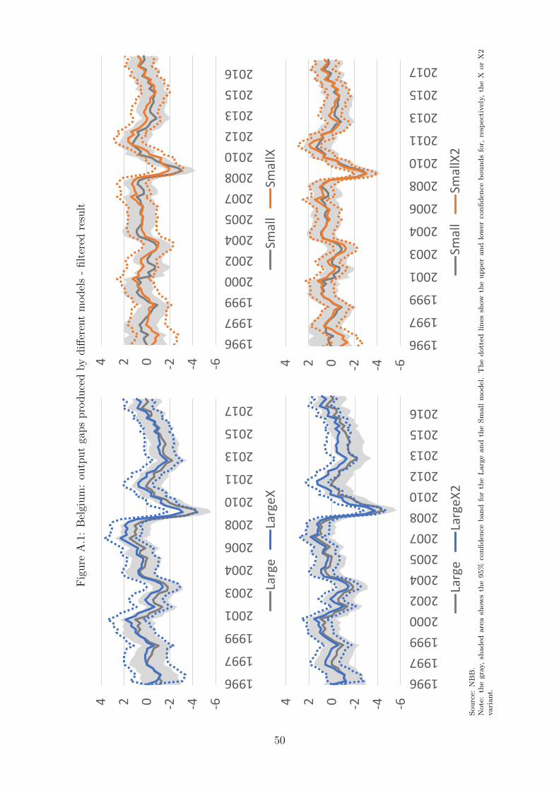
X-model tends to yield a smoother forecast as it does not reach the same peaks and dips
9This is demonstrated by the recursive estimation of the output gaps (i.e. filtered output gaps) thatare available in figure A.1). The smoothed output gaps estimated by all six models are also available inAnnex (figure A.2).
26
as the Large model. More specifically, one noticeable dip in the Large forecast, which is
not produced by Large X (nor by Small), is situated in the first quarter of 2015. Figure
8 demonstrates that the forecast difference at this point is clearly driven by oil. At this
specific point, oil prices dropped by almost 40% on a quarterly basis; the strongest drop
observed since the great recession. Obviously, this oil price movement will not be captured
by the Small model, as it does not include oil among its dependent variables. What is
more remarkable, however, is that the Large X-model incorporates a less negative impact
from oil on the forecast, causing it to remain more stable than the Large. Hence, it seems
that, due to the inclusion of survey information, the short-term forecasts for total inflation
would become less sensitive to oil.
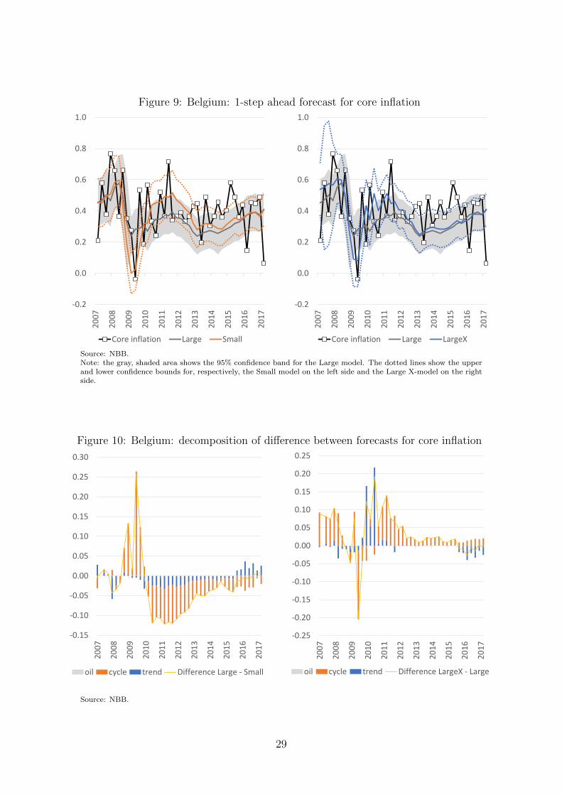
Turning to Belgian core inflation, the left-hand side of figure 9 immediately shows
some interesting results. From 2011 to 2013, the Small forecast lies at the upper confidence
bound of the Large forecast. It is thus consistently higher during this period and, as it
would seem, also closer to the actual outcome for core inflation. The decomposition of
the difference between the forecasts can be found in figure 10. It shows that the Large
forecast has a more negative contribution from the cycle, as well as from the trend, from
2011 onwards. The part of oil prices that is independent from the business cycle does
not have a direct influence on core inflation by construction (cf. equation (14)), which
explains why oil does not appear in the decomposition of the forecast (difference). From
the right-hand side of these figures, we deduct that the forecasts produced by the Large
and the Large X-model are quite similar as of 2012. From 2010 to 2012, however, the
forecast made by Large X demonstrates some more volatility, which relates better to the
actual core inflation.
27
Figure 7: Belgium: 1-step ahead forecast for total inflation
-1.5
-1.0
-0.5
0.0
0.5
1.0
1.5
2.0
20
07
20
08
20
09
20
10
20
11
20
12
20
13
20
14
20
15
20
16
20
17
Total inflation Large Small
-1.5
-1.0
-0.5
0.0
0.5
1.0
1.5
2.0
20
07
20
08
20
09
20
10
20
11
20
12
20
13
20
14
20
15
20
16
20
17
Total inflation Large LargeX
Source: NBB.Note: the gray, shaded area shows the 95% confidence band for the Large model. The dotted lines show the upperand lower confidence bounds for, respectively, the Small model on the left side and the Large X-model on the rightside.
Figure 8: Belgium: decomposition of difference between forecasts for total inflation
-1.0
-0.8
-0.6
-0.4
-0.2
0.0
0.2
0.4
0.6
0.8
1.0
20
07
20
08
20
09
20
10
20
11
20
12
20
13
20
14
20
15
20
16
20
17
oil cycle trend Difference Large - Small
-1.2
-1
-0.8
-0.6
-0.4
-0.2
0
0.2
0.4
0.6
0.8
20
07
20
08
20
09
20
10
20
11
20
12
20
13
20
14
20
15
20
16
20
17
oil cycle trend Difference LargeX - Large
Source: NBB.
28
Figure 9: Belgium: 1-step ahead forecast for core inflation
-0.2
0.0
0.2
0.4
0.6
0.8
1.0
20
07
20
08
20
09
20
10
20
11
20
12
20
13
20
14
20
15
20
16
20
17
Core inflation Large Small
-0.2
0.0
0.2
0.4
0.6
0.8
1.0
20
07
20
08
20
09
20
10
20
11
20
12
20
13
20
14
20
15
20
16
20
17
Core inflation Large LargeX
Source: NBB.Note: the gray, shaded area shows the 95% confidence band for the Large model. The dotted lines show the upperand lower confidence bounds for, respectively, the Small model on the left side and the Large X-model on the rightside.
Figure 10: Belgium: decomposition of difference between forecasts for core inflation
-0.15
-0.10
-0.05
0.00
0.05
0.10
0.15
0.20
0.25
0.30
20
07
20
08
20
09
20
10
20
11
20
12
20
13
20
14
20
15
20
16
20
17
oil cycle trend Difference Large - Small
-0.25
-0.20
-0.15
-0.10
-0.05
0.00
0.05
0.10
0.15
0.20
0.25
20
07
20
08
20
09
20
10
20
11
20
12
20
13
20
14
20
15
20
16
20
17
oil cycle trend Difference LargeX - Large
Source: NBB.
29
Euro area
As regards the 1-step-ahead forecasts for total inflation in the euro area, figure 11
indicates that the Large forecast lies closer to the actual series than the Small forecast.
Remarkably, figure 12 reveals that the difference between these two forecasts is to a
large extent driven by a different estimate for trend inflation, which would have been
generally lower according to the Large model. The forecasts produced by the Large and
Large X-models lie quite close together, although the confidence band around the survey-
augmented model is clearly more moderate. The main differences between the two point
forecasts occur in 2008, 2014 and 2015. For the latter two periods it holds that the Large
forecast incorporates a more negative impact from oil prices. The conclusion is therefore
the same as for Belgium: including survey information appears to temper the weight of oil
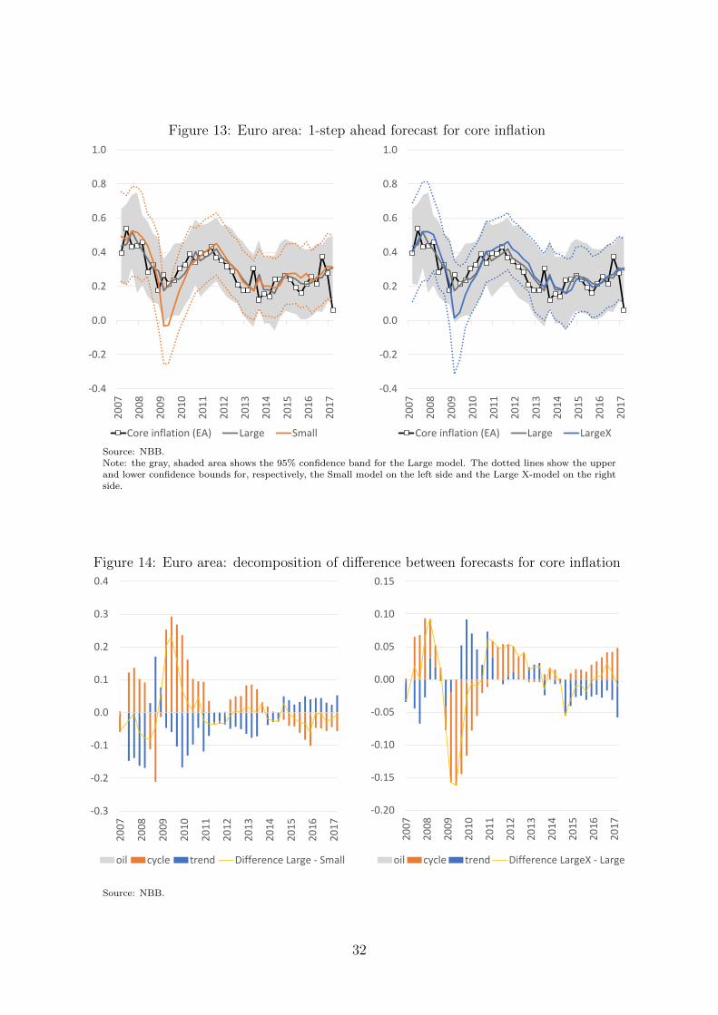
changes on the short-term inflation forecast. Turning to core inflation, it is immediately
clear that the forecast made by the Large model is difficult to beat (cf. figure 13). While
the forecasts produced by the Small, the Large and the Large X differ very little in the
recent period, there is a wide gap during the great recession. In the course of 2009-2010,
both the Small and Large X-model predicted euro area core inflation to be very low,
while this wasn’t actually the case. According to the decomposition (figure 14), this large
difference is mainly due to a different assessment of the cyclical component.
30
Figure 11: Euro area: 1-step ahead forecast for total inflation
-2.0
-1.5
-1.0
-0.5
0.0
0.5
1.0
1.5
2.0
20
07
20
08
20
09
20
10
20
11
20
12
20
13
20
14
20
15
20
16
20
17
Total inflation (EA) Large Small
-2.0
-1.5
-1.0
-0.5
0.0
0.5
1.0
1.5
2.0
20
07
20
08
20
09
20
10
20
11
20
12
20
13
20
14
20
15
20
16
20
17
Total inflation (EA) Large LargeX
Source: NBB.Note: the gray, shaded area shows the 95% confidence band for the Large model. The dotted lines show the upperand lower confidence bounds for, respectively, the Small model on the left side and the Large X-model on the rightside.
Figure 12: Euro area: decomposition of difference between forecasts for total inflation
-1.0
-0.8
-0.6
-0.4
-0.2
0.0
0.2
0.4
0.6
0.8
20
07
20
08
20
09
20
10
20
11
20
12
20
13
20
14
20
15
20
16
20
17
oil cycle trend Difference LargeX - Large
-1.2
-1.0
-0.8
-0.6
-0.4
-0.2
0.0
0.2
0.4
0.6
0.8
1.0
20
07
20
08
20
09
20
10
20
11
20
12
20
13
20
14
20
15
20
16
20
17
oil cycle trend Difference Large - Small
Source: NBB.
31
Figure 13: Euro area: 1-step ahead forecast for core inflation
-0.4
-0.2
0.0
0.2
0.4
0.6
0.8
1.0
20
07
20
08
20
09
20
10
20
11
20
12
20
13
20
14
20
15
20
16
20
17
Core inflation (EA) Large Small
-0.4
-0.2
0.0
0.2
0.4
0.6
0.8
1.0
20
07
20
08
20
09
20
10
20
11
20
12
20
13
20
14
20
15
20
16
20
17
Core inflation (EA) Large LargeX
Source: NBB.Note: the gray, shaded area shows the 95% confidence band for the Large model. The dotted lines show the upperand lower confidence bounds for, respectively, the Small model on the left side and the Large X-model on the rightside.
Figure 14: Euro area: decomposition of difference between forecasts for core inflation
-0.3
-0.2
-0.1
0.0
0.1
0.2
0.3
0.4
20
07
20
08
20
09
20
10
20
11
20
12
20
13
20
14
20
15
20
16
20
17
oil cycle trend Difference Large - Small
-0.20
-0.15
-0.10
-0.05
0.00
0.05
0.10
0.15
20
07
20
08
20
09
20
10
20
11
20
12
20
13
20
14
20
15
20
16
20
17
oil cycle trend Difference LargeX - Large
Source: NBB.
32
5.3 Quantifying forecasting accuracy
The Root Mean Squared Errors (RMSE) can be calculated for the forecast outcomes of
all the models. As a benchmark, the RMSE is calculated for a naıve forecast, similar to
the one put forward by Atkeson and Ohanian (2001), where the expected rate of inflation
equals the sum of observations over the past h quarters. Results will be shown relative
to the naıve RMSE. Ideally, all lines should lie below ’1’, which would indicate that
they perform relatively better than the naıve. It is interesting to note that even if the
corresponding RMSE sometimes lie very close together and their differences are unlikely
to be statistically significant. the previous section has demonstrated some qualitative
differences in the forecasts produced by the models (for example, between the Large and
Small model in figure 9). This may imply that combining certain forecasts may yield
additional information and could further lower the RMSE.
Belgium
Results for Belgium are shown in figure 15, relative against the naıve benchmark for
different horizons, so values smaller than one imply that our model is more accurate
than the benchmark. When it comes to total inflation, the gain from including survey
information in the forecasting model seems limited at first sight, as the most accurate
forecasts are produced by the large model without survey expectations. However, keep in
mind that the graph displays expected inflation cumulated over the forecasting horizon
and the accuracy of the Large and Large X-models mainly (or only) differs at the shortest
horizon. This suggests that the two-steps-ahead forecast from Large X is actually more
accurate than the one coming from Large.
Forecasts for core inflation, on the other hand, could benefit more clearly from the
inclusion of survey information, as the dotted lines (expectations-augmented models) lie
beneath the full lines (models that include no surveys).
Euro area
Figure 16 shows the relative forecasting accuracy of the models for the euro area
inflation rates. For both total and core inflation, Large delivers the most accurate forecasts
over the evaluation period. The usefulness of survey information seems less clear than in
the Belgian case: models augmented with expectations (X or X2) are generally unable
to further improve the forecasting accuracy. Also, as indicated by the right-hand side of
33
Figure 15: Belgium: relative RMSE for six models for total and core inflation
0.6
0.7
0.8
0.9
1.0
1.1
0Q 1Q 2Q 3Q 4Q
Total inflation
Small SmallX SmallX2 Large LargeX LargeX2
0.6
0.7
0.8
0.9
1.0
0Q 1Q 2Q 3Q 4Q
Core inflation
Source: NBB.
Note: the forecast evaluation period runs from 2007Q4 to 2017Q4.
the graph, only the Large model manages to outperform the naıve benchmark for core
inflation.
5.4 Adding noise: AR(1) measurement errors in the two survey
equations
Model consistency may impose a very strict restriction on the way survey data is exploited.
First, in the presence of model misspecification, it may not be a good idea to link the
surveys with forecasts coming from the (possibly misspecified) model. Second, even if
model misspecification would be small, our qualitative measures of inflation expectations
are a sum of balances where the respondents are simply asked to produce a binary output,
i.e. “prices will go up” vs “prices will go down”. In this context, it may be too much to
expect that the balance of responses will exactly match a quantitative measure of inflation
expectations that can be made consistent with the model.
By including autocorrelated measurement errors that are orthogonal to all factors,
we aim to re-interpret the fluctuations in the surveys according to their correlation with
the model factors. This way, less weight would be attributed to fitting the surveys in a
34
Figure 16: Euro area: relative RMSE for six models for total and core inflation
0.6
0.7
0.8
0.9
1.0
0Q 1Q 2Q 3Q 4Q
Total inflation (EA)
Small SmallX SmallX2 Large LargeX LargeX2
0.5
0.7
0.9
1.1
1.3
1.5
1.7
0Q 1Q 2Q 3Q 4Q
Core inflation (EA)
Source: NBB.Note: the forecast evaluation period runs from 2007Q4 to 2017Q4.
model-consistent way.
As shown by the blue line in figure 17, for Belgium, this new specification (called “X
noise”) does typically not improve the accuracy of the Large X-model, with the exception
of the current period forecast for total inflation. It is likely that, in the alternative model,
by allowing for more noise in the measurement equation of the surveys, the role of the
surveys decreases in favour of the hard data on oil prices, which in Belgium is highly
correlated with headline inflation. This would explain why the current-quarter forecast
of the model with noise is more accurate for total inflation, where we found earlier that
surveys tend to diminish the weight given to oil price changes (cf. Section 5.2).
For the euro area, the alternative model allowing for persistent measurement errors
consistently outperforms the Large X-model, while it only manages to outperform the
Large model without any survey information at the horizons 0 and 1 (figure 18).
35
Figure 17: Belgium: sensitivity analysis of large models
0.6
0.7
0.8
0.9
1.0
0Q 1Q 2Q 3Q 4Q
Total inflation (BE)
Large LargeX LargeX_noise
0.6
0.7
0.8
0.9
1.0
0Q 1Q 2Q 3Q 4Q
Core inflation (BE)
Source: NBB.
Figure 18: Euro area: sensitivity analysis of large models
0.7
0.8
0.9
1.0
0Q 1Q 2Q 3Q 4Q
Total inflation (EA)
Large LargeX LargeX_noise
0.5
0.6
0.7
0.8
0.9
1.0
1.1
1.2
1.3
0Q 1Q 2Q 3Q 4Q
Core inflation (EA)
Source: NBB.
36
6 Focus on the recent period and interpretation
6.1 A change in the forecast evaluation sample
Our pseudo out-of-sample evaluation suggests that the reported differences in accuracy
are related to a few outliers during the great recession period. Figure 13, in particular,
illustrated the large differences in performance over three consecutive quarters alone. This
section evaluates how our results (and conclusions) may change if we focus on the most
recent period only and start evaluating the forecasts as of 2012. After all, this is the
period that is of most interest to us: due to the appearance of inflation (forecast) puzzles,
we wanted to investigate the usefulness of surveys. Results are shown in figures 19 and
20.
For Belgian core inflation, the conclusion remains that the survey-augmented models
are more accurate. However, while before the Large and Small models were found to be
equally accurate, the Small model prevails when focusing on the shorter evaluation sample.
For Belgian total inflation, the shorter evaluation sample could lead us to conclude that
adding surveys could be beneficial (in case of the Large model).
Turning to the euro area, the survey-augmented X2-models for total inflation seem
to beat the Large model, when the forecasting horizon reaches at least 1 quarter ahead.
Also for core inflation, the Large X2-model is found to be somewhat more accurate than
the Large over this specific evaluation sample.
As the differences in RMSE’s can be very little, it is worth looking at the actual
forecasts. More specifically, we investigate 4-steps-ahead forecasts for total and core
inflation, for Belgium and the euro area respectively. Inflation rates and forecasts are
cumulated over 4 periods, in order to make the differences clear on a graph. Figure 21
is mainly interesting from the perspective of core inflation (on the right-hand side of the
graph). It is visually immediately clear that the Large model performs best during the
great recession. However, in the most recent period, say as of early 2013, the Large X2-
model is actually consistently (much) closer to the actual core inflation in Belgium. This
figure thereby also illustrates the “missing low inflation puzzle” for Belgium, because all
forecasts were significantly below the actual outcome in the recent period. One would
have expected (core) inflation to be much lower than it turned out. While the puzzle
37
Figure 19: Belgium: relative RMSE for six models for total and core inflation (robustness)
0.5
0.6
0.7
0.8
0.9
1.0
0Q 1Q 2Q 3Q 4Q
Total inflation (BE)
Small SmallX SmallX2 Large LargeX LargeX2
0.6
0.8
1.0
1.2
1.4
1.6
0Q 1Q 2Q 3Q 4Q
Core inflation (BE)
Source: NBB.
Note: the forecast evaluation period for the robustness exercise runs from 2012Q1 to 2017Q4.
Figure 20: Euro area: relative RMSE for six models for total and core inflation (robust-ness)
0.4
0.5
0.6
0.7
0.8
0.9
0Q 1Q 2Q 3Q 4Q
Total inflation (EA)
Small SmallX SmallX2 Large LargeX LargeX2
0.5
0.8
1.1
1.4
0Q 1Q 2Q 3Q 4Q
Core inflation (EA)
Source: NBB.
Note: the forecast evaluation period for the robustness exercise runs from 2012Q1 to 2017Q4.
38
cannot be completely solved using survey information, adding this source of information
does help. For Belgian total inflation, the forecasts incorporating survey information only
clearly prevail as of 2015.
For the euro area, total inflation as of 2011 is best approximated by models containing
surveys; either in a model-consistent way (X) or in a looser way (X2). The forecasting
puzzle here is different than for Belgian core inflation: forecasts for euro area inflation
were generally too positive during 2013-2016 and inflation surprised on the downside. For
euro area core inflation, there is no obvious forecasting puzzle, yet forecasts made by the
Large X2-model seem to end up closest to the actual inflation rates between 2012 and
Now that the previous sections have established that, at least for certain periods, survey
information may be useful for the purpose of inflation forecasting, one may wonder which
of the two surveys is yielding the most relevant information: is it the business or the
consumer survey?
39
Figure 22: Euro area: 4-steps ahead inflation forecasts (cumulated figures)
-1.0
-0.5
0.0
0.5
1.0
1.5
2.0
2.5
3.0
3.5
4.02
00
8
20
09
20
10
20
11
20
12
20
13
20
14
20
15
20
16
20
17
Total inflation (EA) Large
LargeX LargeX2
-0.5
0.0
0.5
1.0
1.5
2.0
2.5
20
08
20
09
20
10
20
11
20
12
20
13
20
14
20
15
20
16
20
17
Core inflation (EA) Large
LargeX LargeX2
Source: NBB.
Figure 23: Belgium: relative RMSE of survey-augmented models (business versus con-sumer surveys)
0.6
0.7
0.8
0.9
1.0
0Q 1Q 2Q 3Q 4Q
Total inflation
Large LargeX BE_LargeX_Bonly BE_LargeX_Conly
0.6
0.7
0.8
0.9
1.0
0Q 1Q 2Q 3Q 4Q
Core inflation
Source: NBB.Note: The forecast evaluation period runs from 2007Q4 to 2017Q4. Bonly and Conly represent the case in whichthe model is augmented with survey information from businesses, respectively consumers, only.
40
For Belgian core inflation, accuracy gains realized by Large X mostly come from the
short-term price expectations in the business surveys. The model that includes business
expectations only (“Bonly” in figure 23) is about as accurate as the normal Large X-model,
while the model that includes consumer expectations only (“Conly”) clearly delivers a less
accurate forecast. This suggests that disregarding the readily available survey information
from price-setters leads to sub-optimal inflation projections.
While for the euro area, the added value from surveys is less clear than for Belgium,
figure 24 yields the same conclusion as in the Belgian case. If anything, survey information
from businesses (“Bonly”) tends to improve the forecasting accuracy most.
Figure 24: Euro area: relative RMSE of survey-augmented models (business versus con-sumer surveys)
0.65
0.75
0.85
0.95
0Q 1Q 2Q 3Q 4Q
Total inflation (EA)
Large LargeX LargeX_Bonly LargeX_Conly
0.5
0.6
0.7
0.8
0.9
1.0
1.1
1.2
1.3
0Q 1Q 2Q 3Q 4Q
Core inflation (EA)
Source: NBB.Note: The forecast evaluation period runs from 2007Q4 to 2017Q4. Bonly and Conly represent the case in whichthe model is augmented with survey information from businesses, respectively consumers, only.
41
7 Conclusion
The motivation for this paper can be traced back to the recent difficulties in correctly
forecasting inflation developments, in particular using models based on the Phillips Curve.
In this connection, the euro area and Belgium are interesting cases as inflation typically
turned out lower than expected in the euro area, while the opposite was true for Belgium.
Several studies have tried to gauge the usefulness of including measures of inflation
expectations in forecasting models and have found mixed results. However, the literature
has mostly focused on indicators derived from financial markets, inflation estimates of
professional forecasters and, to a lesser extent, expectations in consumer surveys. In this
paper we use qualitative information from both consumer and business surveys that are
harmonised at the EU level. Consumers are asked about the development of consumer
prices over the next twelve months while respondents to the business survey have to
indicate whether or not they expect increases in selling prices over the next quarter. We
argue that, in both cases, the balance of replies can provide useful information, on a
monthly basis, regarding inflation expectations.
With a view to formally testing the information content of these survey indicators for
inflation projections, we develop a suite of unobserved component models for both the euro
area and Belgium. In some models, surveys are linked to the expectations derived from the
model, while in others, they are simply added to the information set while imposing weaker
forms of model consistency. We specifically include headline as well as core inflation and
assess whether adding the survey information on expected price changes leads to accuracy
gains. Results are mixed if one considers the whole evaluation period covering the last
ten years. For Belgium, surveys do not help to explain total inflation: the larger models
that also explicitly take into account the oil price and the price mark-up, but not the
survey information on prices are the most accurate. As regards core inflation estimates,
surveys do seem to matter and we specifically show that it is the business survey that is
driving this result. However, for the euro area, adding price expectations from surveys to
the models does not improve their accuracy. All in all, we do not find convincing evidence
that shows that survey information can always inform inflation projections.
However, a focus on the most recent period alters the conclusion. If the evaluation
sample is restricted to the period starting in 2012 only, models that include the survey
42
expectations on prices tend to outperform similar models that don’t, both for Belgium
and the euro area. This may suggest that, specifically in periods where structural models
fail to account for actual developments, such as in the recent ones, price expectations from
business surveys in particular could provide information that can be used to improve the
forecasts. Our paper just presents one modelling approach that allows to combine struc-
tural drivers of inflation with survey information. Further research is definitely necessary
to assess the best manner to include survey information in actual forecasting models (the
design and structure of which may depend on the horizon considered). Our results suggest
that it may be worthwhile to explore that option.
Another avenue for further research relates to the more formal identification of the
periods for which survey information could improve the accuracy of the projections, or –
to put it differently – for which the accuracy of the traditional models is particularly low.
One tentative interpretation of the recent episode is that this may pertain to significant
changes in underlying cost drivers and the misspecification of the pass-through to final
prices. At least for the Belgian case, a slower pass-through of the policy-driven moderation
in labour costs (as also evidenced by very dynamic profit margins around that time) has
definitely contributed to keeping inflation high. To the extent that the business survey
measures the expectations of the actual price-setters, they could specifically inform about
the planned pass-through of changes in costs that may be different from the one included
in the structural models that are routinely used for forecasting.
43
References
[1] Atkeson, A. and L.E. Ohanian (2001), Are Phillips curves useful for forecasting in-
flation?, Federal Reserve Bank of Minneapolis Quarterly Review, Win, 2-11.
[2] Ang, A., G. Bekaert and M. Wei (2007), Do macro variables, asset markets, or surveys
forecast inflation better?, Journal of Monetary Economics, 4, 1163-1212.
[3] Basselier, R., D. de Antonio Liedo and G. Langenus (2018), Nowcasting real economic
activity in the euro area : Assessing the impact of qualitative surveys, Journal of
Business Cycle Research,14, 1-46
[4] Bernanke, B.S. (2007), Inflation expectations and inflation forecasting, speech given
at the Monetary Economics Workshop of the National Bureau of Economic Research
Summer Institute, Cambridge, Massachusetts, July 10, 2007.
[5] Brockwell, P.J. and R.A. Davis (1987), Time Series: Theory and Models, New York:
Springer-Verlag .
[6] Carlson, J.A. and M. Parkin (1975), Inflation Expectations, Economica, 42 (166),
123-138.
[7] Carroll, C. (2003), Macroeconomic expectations of households and professional fore-
casters, The Quarterly Journal of Economics, 118 (1), 269-298.
[8] Chan, J., G. Koop and S. Potter (2016), A Bounded Model of Time Variation in
Trend Inflation, Nairu and the Phillips Curve, Journal of Applied Econometrics, 31
(3), 551-565.
[9] Coibion, O. and Y. Gorodnichenko (2015), Is the Phillips Curve Alive and Well
after All? Inflation Expectations and the Missing Disinflation, American Economic
Journal: Macroeconomics, 7 (1), 197-232.
[10] Coibion, O., Y. Gorodnichenko and R. Kamdar (2018), How Do Firms Form Their
Expectations? New Survey Evidence, Forthcoming in American Economic Review
44
[11] de Antonio Liedo, D. (2015), Nowcasting Belgium, National Bank of Belgium, Eu-
rostat Review of National Accounts and Macroeconomic Indicator, Special Issue on
New Techniques and Technologies for Statistics 2, 7-41.
[12] ECB (2007), Recent developments in consumers’ inflation perceptions and expecta-
tions in the euro area, ECB Monthly Bulletin, November 2007, 38-41.
[13] Ehrmann, M., D. Pfajfar and E. Santoro (2017), Consumers’ Attitudes and Their
Inflation Expectations, International Journal of Central Banking, 13 (1), 225-259.
[14] Forsells, M. and G. Kenny (2004), Survey expectations, rationality and the dynamics
of euro area inflation, Journal of Business cycle measurement and analysis, 1, 13-41.
[15] Francke, M.K., S.J. Koopman, and A.F. de Vos (2010), Likelihood functions for
state space models with diffuse initial conditions, Journal of Time Series Analysis,
31, 407-414.
[16] Geweke, J. (1977), The Dynamic Factor Analysis of Economic Time Series. In:
Aigner, D.J. and Goldberger, A.S., Eds., Latent Variables in Socio-Economic Models
1, North-Holland, Amsterdam.
[17] Harvey, A. (1985), Trends and Cycles in Macroeconomic Time Series, Journal of
Business and Economic Statistics, 3 (3), 216-227.
[18] Hasenzagl, T., F. Pellegrino, L. Reichlin and G. Ricco (2018), A model of the FED’s
view on inflation, Sciences PO OFCE Working Paper, 03.
[19] Mankiw, NG., R. Reis and J. Wolfers (2004), Disagreement about inflation expecta-
autoregressive-moving average process, Biometrika, 67, 232-233.
[20] Sargent, T.J. and C.A. Sims (1977), Business cycle modeling without pretending
to have too much a priori economic theory, Federal Reserve Bank of Minneapolis,
Working Paper 55.
[21] Scheufele, R. (2011), Are qualitative inflation expectations useful to predict infla-
tion?, Journal of Business Cycle Measurement and Analysis, 2, 29-53.
45
[22] Souleles, N.S. (2004), Expectations, Heterogeneous Forecast Errors and Consump-
tion: Micro Evidence from the Michigan Consumer Sentiment Surveys, Inflation
Expectations, 36 (1), 39-72.
[23] Stella, A. and J.H. Stock (2013), A State-Dependent Model for Inflation Forecasting,
FRB International Finance Discussion Paper, 1062.
[24] Stockhammer, P. and P. Osterholm (2016), Do inflation expectations Granger cause
inflation?, National institute of economic research working paper, 145.
[25] Thum-Thysen, A. and E. Canton (2015), Estimation of service sector mark-ups de-
termined by structural reform indicators, European Commission, Economic Papers
547.
46
8 Annexes
Equation (A.1): State-Space form of the Large X-UCM: measurement equation . . . . . .48
Equation (A.2): State-Space form of the Large X-UCM: transition equation . . . . . . . . . 49
Figure A.1: Belgium: output gaps produced by different models - filtered result . . . . . 50
Figure A.2: Belgium: output gaps produced by different models - smoothed result . . . 51
Figure A.3: Euro area: output gaps produced by different models - filtered result . . . . 52
47
Sta
te-S
pac
efo
rmof
the
Lar
geX
-UC
M:
mea
sure
men
teq
uat
ion
Ut
Yt
πt
πcore
t
πM t
Poil
t
µYoY
t
Sy t
SB t
SC t
=
mu
my
mπ
mcore
mm
moil
mµ
ms
mb
mc
+
10
00
00
00
01
00
00
00
0
00
10
00
00
0κ
00
00
00
0
00
00
10
00
0λπ
00
00
ζ π0
0
00
00
01
00
00
00
0λcore
00
0
00
00
00
10
0λM
00
00
ζ M0
φM
00
00
00
01
0λOil
00
00
ζ Oil
00
00
00
00
00
0λµ
00
0−λµ
00
0
00
00
00
00
0κS
00
0−κS
00
0
00
00
00
00
0Λ
1Λ
20
00
Z1
Z2
0
00
00
00
00
0Λ
∗ 1Λ
∗ 20
00
Z∗ 1
Z∗ 2
0
τU t τU t−
1
τY t τY t−
1
τπ t τcore
t τM t τOil
t τOil
t−1
δ t δ t−
1
δ t−
2
δ t−
3
δ t−
4
ϑt
ϑt−
1
ξM t
+
ηU t ηY t ηπ t ηcore
t ηM t ηoilt ηµ t ηBC
S,t
ηB S,t
ηC S,t
(A.1
)
48
Sta
te-S
pac
efo
rmof
the
Lar
geX
-UC
M:
tran
siti
oneq
uat
ion
τU t τU t−
1
τY t τY t−
1
τπ t τcore
t τM t τOil
t τOil
t−1
δ t δ t−1
δ t−2
δ t−3
δ t−4
ϑt
ϑt−
1
ξM t
=
0 0 0 0 0 0 0 c oil
0 0 0 0 0 0 0 0 0 0
+
2−
10
00
00
00
00
00
00
00
10
00
00
00
00
00
00
00
0
00
2−
10
00
00
00
00
00
00
00
10
00
00
00
00
00
00
0
00
00
10
00
00
00
00
00
0
00
00
01
00
00
00
00
00
0
00
00
00
10
00
00
00
00
0
00
00
00
01
00
00
00
00
0
00
00
00
00
10
00
00
00
0
00
00
00
00
0α1
α2
00
00
00
00
00
00
00
01
00
00
00
0
00
00
00
00
00
10
00
00
0
00
00
00
00
00
01
00
00
0
00
00
00
00
00
00
10
00
0
00
00
00
00
00
00
00
ρ1
ρ2
0
00
00
00
00
00
00
00
10
0
00
00
00
00
00
00
00
00
ρM
τU t−
1
τU t−
2
τY t−
1
τY t−
2
τπ t−
1
τcore
t−2
τM t−
1
τOil
t−1
δ t−1
δ t−2
δ t−3
δ t−4
δ t−5
ϑt−
1
ϑt−
2
ξM t−
1
+
εU t 0 εY t 0 επ t εcore
t εM t εOil
t ζϑ t 0 0 0 0 ζϑ t 0 eM t
(A.2
)
Model
consi
sten
cy(X
)im
plies
:
Λ1
=f
(αBλπ,α
1),
Λ2
=f
(αBλπ,α
2)
Z1
=f
(αBζ pi,ρ
1),Z2
=f
(αBζ pi,ρ
2)
Λ∗ 1
=f
(αBλπ,α
1,α
2),
Λ∗ 2
=f
(αBλπ,α
1,α
2)
Z∗ 1
=f
(αBζ pi,ρ
1,ρ
2),Z
∗ 2=f
(αBζ pi,ρ
1,ρ
2)
49
Fig
ure
A.1
:B
elgi
um
:ou
tput
gaps
pro
duce
dby
diff
eren
tm
odel
s-
filt
ered
resu
lt
-6-4-20241996
1997
1999
2001
2003
2004
2006
2008
2010
2011
2013
2015
2017
Large
LargeX
-6-4-2024
1996
1997
1999
2000
2002
2004
2005
2007
2008
2010
2012
2013
2015
2016
Large
LargeX
2
-6-4-2024
1996
1997
1999
2000
2002
2004
2005
2007
2008
2010
2012
2013
2015
2016
Small
SmallX
-6-4-2024
1996
1997
1999
2001
2003
2004
2006
2008
2010
2011
2013
2015
2017
Small
SmallX2
Sou
rce:
NB
B.
Note
:th
egra
y,sh
ad
edare
ash
ow
sth
e95%
con
fid
ence
ban
dfo
rth
eL
arg
ean
dth
eS
mall
mod
el.
Th
ed
ott
edlin
essh
ow
the
up
per
an
dlo
wer
con
fid
ence
bou
nd
sfo
r,re
spec
tivel
y,th
eX
or
X2
vari
ant.
50
Fig
ure
A.2
:B
elgi
um
:ou
tput
gaps
pro
duce
dby
diff
eren
tm
odel
s-
smoot
hed
resu
lt
-4-20246
1995
1997
1998
2000
2002
2004
2006
2008
2009
2011
2013
2015
2017
Large
LargeX
2
-4-202461995
1997
1998
2000
2002
2004
2006
2008
2009
2011
2013
2015
2017
Large
LargeX
-4-2024
1995
1997
1998
2000
2002
2004
2006
2008
2009
2011
2013
2015
2017
Small
SmallX
-4-2024
1995
1997
1998
2000
2002
2004
2006
2008
2009
2011
2013
2015
2017
Small
SmallX2
Sou
rce:
NB
B.
Note
:th
egra
y,sh
ad
edare
ash
ow
sth
e95%
con
fid
ence
ban
dfo
rth
eL
arg
ean
dth
eS
mall
mod
el.
Th
ed
ott
edlin
essh
ow
the
up
per
an
dlo
wer
con
fid
ence
bou
nd
sfo
r,re
spec
tivel
y,th
eX
or
X2
vari
ant.
51
Fig
ure
A.3
:E
uro
area
:ou
tput
gaps
pro
duce
dby
diff
eren
tm
odel
s-
filt
ered
resu
lt
-12-8-4048
12
1996
1997
1999
2001
2003
2004
2006
2008
2010
2011
2013
2015
2017
Large
LargeX
-12-8-4048
12
1996
1997
1999
2001
2003
2004
2006
2008
2010
2011
2013
2015
2017
Large
LargeX
2
-8-4048
1996
1997
1999
2001
2003
2004
2006
2008
2010
2011
2013
2015
2017
Small
SmallX
-12-8-4048
1996
1997
1999
2001
2003
2004
2006
2008
2010
2011
2013
2015
2017
Small
SmallX2
Sou
rce:
NB
B.
Note
:th
egra
y,sh
ad
edare
ash
ow
sth
e95%
con
fid
ence
ban
dfo
rth
eL
arg
ean
dth
eS
mall
mod
el.
Th
ed
ott
edlin
essh
ow
the
up
per
an
dlo
wer
con
fid
ence
bou
nd
sfo
r,re
spec
tivel
y,th
eX
or
X2
vari
ant.
52
NBB WORKING PAPER No. 348 – OCTOBER 2018 53
NATIONAL BANK OF BELGIUM - WORKING PAPERS SERIES
The Working Papers are available on the website of the Bank: http://www.nbb.be.
302. “The transmission mechanism of credit support policies in the Euro Area”, by J. Boeckx, M. de Sola Pereaand G. Peersman, Research series, October 2016.
303. “Bank capital (requirements) and credit supply: Evidence from pillar 2 decisions”, by O. De Jonghe,H. Dewachter and S. Ongena, Research series, October 2016.
304. “Monetary and macroprudential policy games in a monetary union”, by R. Dennis and P. Ilbas, Researchseries, October 2016.
305. “Forward guidance, quantitative easing, or both?, by F. De Graeve and K. Theodoridis, Research series,October 2016.
306. “The impact of sectoral macroprudential capital requirements on mortgage loan pricing: Evidence from theBelgian risk weight add-on”, by S. Ferrari, M. Pirovano and P. Rovira Kaltwasser, Research series, October2016.
307. “Assessing the role of interbank network structure in business and financial cycle analysis”, by J-Y Gnaboand N.K. Scholtes, Research series, October 2016.
308. “The trade-off between monetary policy and bank stability”, by M. Lamers, F. Mergaerts, E. Meuleman andR. Vander Vennet, Research series, October 2016.
309. “The response of euro area sovereign spreads to the ECB unconventional monetary policies”, byH. Dewachter, L. Iania and J-C. Wijnandts, Research series, October 2016.
310. “The interdependence of monetary and macroprudential policy under the zero lower bound”, by V. Lewisand S. Villa, Research series, October 2016.
311. “The impact of exporting on SME capital structure and debt maturity choices”, by E. Maes,N. Dewaelheynes, C. Fuss and C. Van Hulle, Research series, October 2016.
312. “Heterogeneous firms and the micro origins of aggregate fluctuations”, by G. Magerman, K. De Bruyne, E.Dhyne and J. Van Hove, Research series, October 2016.
313. “A dynamic factor model for forecasting house prices in Belgium”, by M. Emiris, Research series,November 2016.
314. “La Belgique et l’Europe dans la tourmente monétaire des années 1970 – Entretiens avec Jacques vanYpersele”, by I. Maes and S. Péters, Research series, December 2016.
315. “Creating associations to substitute banks’ direct credit. Evidence from Belgium”, by M. Bedayo, Researchseries, December 2016.
316. “The impact of export promotion on export market entry”, by A. Schminke and J. Van Biesebroeck,Research series, December 2016.
317. “An estimated two-country EA-US model with limited exchange rate pass-through”, by G. de Walque,Ph. Jeanfils, T. Lejeune, Y. Rychalovska and R. Wouters, Research series, March 2017.
318. Using bank loans as collateral in Europe: The role of liquidity and funding purposes”, by F. Koulischer andP. Van Roy, Research series, April 2017.
319. “The impact of service and goods offshoring on employment: Firm-level evidence”, by C. Ornaghi,I. Van Beveren and S. Vanormelingen, Research series, May 2017.
320. “On the estimation of panel fiscal reaction functions: Heterogeneity or fiscal fatigue?”, by G. Everaert andS. Jansen, Research series, June 2017.
321. “Economic importance of the Belgian ports: Flemish maritime ports, Liège port complex and the port ofBrussels - Report 2015”, by C. Mathys, Document series, June 2017.
322. “Foreign banks as shock absorbers in the financial crisis?”, by G. Barboni, Research series, June 2017.323. “The IMF and precautionary lending: An empirical evaluation of the selectivity and effectiveness of the
flexible credit line”, by D. Essers and S. Ide, Research series, June 2017.324. “Economic importance of air transport and airport activities in Belgium – Report 2015”, by S. Vennix,
Document series, July 2017.325. “Economic importance of the logistics sector in Belgium”, by H. De Doncker, Document series, July 2017.326. “Identifying the provisioning policies of Belgian banks”, by E. Arbak, Research series, July 2017.327. “The impact of the mortgage interest and capital deduction scheme on the Belgian mortgage market”, by
A. Hoebeeck and K. Inghelbrecht, Research series, September 2017.
328. “Firm heterogeneity and aggregate business services exports: Micro evidence from Belgium, France,Germany and Spain”, by A. Ariu, E. Biewen, S. Blank, G. Gaulier, M.J. González, Ph. Meinen, D. Mirza,C. Martín and P. Tello, Research series, September 2017.
329. “The interconnections between services and goods trade at the firm-level”, by A. Ariu, H. Breinlichz,G. Corcosx, G. Mion, Research series, October 2017.
54 NBB WORKING PAPER No. 348 – OCTOBER 2018
330. “Why do manufacturing firms produce services? Evidence for the servitization paradox in Belgium”, byP. Blanchard, C. Fuss and C. Mathieu, Research series, November 2017.
331. “Nowcasting real economic activity in the euro area: Assessing the impact of qualitative surveys”, byR. Basselier, D. de Antonio Liedo and G. Langenus, Research series, December 2017.
332. “Pockets of risk in the Belgian mortgage market: Evidence from the Household Finance and ConsumptionSurvey (HFCS)”, by Ph. Du Caju, Research series, December 2017.
333. “The employment consequences of SMEs’ credit constraints in the wake of the great recession” byD. Cornille, F. Rycx and I. Tojerow, Research series, December 2017.
334. “Exchange rate movements, firm-level exports and heterogeneity”, by A. Berthou and E. Dhyne, Researchseries, January 2018.
335 “Nonparametric identification of unobserved technological heterogeneity in production”, by L. Cherchye,T. Demuynck, B. De Rock and M. Verschelde, Research series, February 2018.
336 “Compositional changes in aggregate productivity in an era of globalisation and financial crisis”, by C. Fussand A. Theodorakopoulos, Research series, February 2018.
337. “Decomposing firm-product appeal: How important is consumer taste?”, by B. Y. Aw, Y. Lee andH. Vandenbussche, Research series, March 2018.
338 “Sensitivity of credit risk stress test results: Modelling issues with an application to Belgium”, byP. Van Roy, S. Ferrari and C. Vespro, Research series, March 2018.
339. “Paul van Zeeland and the first decade of the US Federal Reserve System: The analysis from a Europeancentral banker who was a student of Kemmerer”, by I. Maes and R. Gomez Betancourt, Research series,March 2018.
340. “One way to the top: How services boost the demand for goods”, by A. Ariu, F. Mayneris and M. Parenti,Research series, March 2018.
341 “Alexandre Lamfalussy and the monetary policy debates among central bankers during the Great Inflation”,by I. Maes and P. Clement, Research series, April 2018.
342. “The economic importance of the Belgian ports: Flemish maritime ports, Liège port complex and the portof Brussels – Report 2016”, by F. Coppens, C. Mathys, J.-P. Merckx, P. Ringoot and M. Van Kerckhoven,Document series, April 2018.
343. “The unemployment impact of product and labour market regulation: Evidence from European countries”,by C. Piton, Research series, June 2018.
344. “Trade and domestic production networks”, by F. Tintelnot, A. Ken Kikkawa, M. Mogstad, E. Dhyne,Research series, September 2018.
345. “Review essay: Central banking through the centuries”, by I. Maes, Research series, October 2018.346 “IT and productivity: A firm level analysis”, by E. Dhyne, J. Konings, J. Van den Bosch, S. Vanormelingen,
Research series, October 2018.347 “Identifying credit supply shocks with bank-firm data: methods and applications”, by H. Degryse,
O. De Jonghe, S. Jakovljević, Klaas Mulier, Glenn Schepens, Research series, October 2018.348 “Can inflation expectations in business or consumer surveys improve inflation forecasts?”, by R. Basselier,
D. de Antonio Liedo, J. Jonckheere and G. Langenus, Research series, October 2018.
Layout : Analysis and Research Group Cover : NBB AG – Prepress & Image
Published in October 2018
Editor
Jan SmetsGovernor of the National Bank of Belgium
National Bank of Belgium Limited liability company RLP Brussels – Company’s number : 0203.201.340 Registered office : boulevard de Berlaimont 14 – BE -1000 Brussels www.nbb.be