Accident Analysis and Prevention 59 (2013) 301– 308
Contents lists available at ScienceDirect
Accident Analysis and Prevention
journa l h om epage: www.elsev ier .com/ locate /aap
an it be true that most drivers are safer than the average driver?
une Elvik ∗
nstitute of Transport Economics, Gaustadalleen 21, NO-0349 Oslo, Norway
r t i c l e i n f o
rticle history:eceived 10 March 2013eceived in revised form 5 June 2013ccepted 19 June 2013
eywords:river safetyptimism bias
a b s t r a c t
Surveys finding that a large majority of drivers regard themselves as safer than the average driver havebeen ridiculed as showing that most drivers are overconfident about their safety and as showing some-thing which is logically impossible, since in a normal distribution exactly half are below average and halfabove. This paper shows that this criticism is misplaced. Driver accident involvement does not follow anormal distribution, and it is mathematically entirely possible that a huge majority of drivers could besafer than the average driver. The distribution of accidents in a population of drivers is typically skewed,with a majority of drivers not reporting involvement in any accident in the period covered by the data,
egression-to-the-meanong-term expected number of accidentsegative binomial distribution
often a period of 1–3 years. In this paper, examples are given of data sets in which the percentage ofdrivers who are safer than the average driver ranges from about 70% to 90%. The paper explains how,based on knowing the mean and variance of the distribution of accidents in a population of drivers in agiven period, the long-term expected number of accidents for drivers who were involved in 0, 1, 2, ormore accidents can be estimated. Such estimates invariably show that the huge majority of drivers aresafer than the average driver.
. Introduction
In 1981 Ola Svenson published a much-quoted paper entitled:Are we all less risky and more skilful than our fellow drivers?”Svenson, 1981). In the paper, he asked students in the United Statesnd Sweden to place themselves in percentiles with respect to driv-ng skill and safety. Ten percentiles (0–10, 11–20, etc.) were listed.he percentiles were ranked so that the first (0–10) indicated theottom 10% with respect to skill and safety and the last (91–100) thepper 10% with respect to skill and safety. If students had a real-
stic perception of their skill and safety, then, by definition, eachercentile should contain 10% of the students. However, Svensonound that 87.5% of US students and 77.1% of Swedish students ratedheir safety in the upper five percentiles, i.e. safer than the median50th percentile) driver.
Similar results have been reproduced in subsequent studies (see,or example, Svenson et al., 1985; DeJoy, 1989; Holland, 1993; Harrénd Sibley, 2007) and interpreted as showing “optimism bias”.ome authors seem to assume that it is mathematically impossibleor more than half of drivers to be safer than average. Thus, Svenson,ishhoff and MacGregor state (1985, page 119): “Of course, it is no
ore possible for most people to be safer than average than it is forost to have above average intelligence.” Hence, when more than
0% of drivers state that they are safer than the average driver this
is interpreted as showing a biased perception of driver safety. It is,however, entirely possible that more than 50% of drivers actuallyare safer than the average driver. The aim of this paper is to showthat in representative samples of drivers, it will typically be the casethat:
1. A large majority of drivers will not report involvement in anaccident during a period of a few years (like 1–3 years).
2. The long-term expected number of accidents for drivers whoreported involvement in 0, 1, 2, or more accidents can be esti-mated if the mean number of accidents per driver and itsvariance in the population of drivers are known.
3. It will typically be the case that a huge majority of drivers have along-term expected number of accidents which is slightly lowerthan the overall mean number of accidents per driver whereasa small minority of drivers have a long-term expected numberof accidents which is considerably higher than the overall meannumber of accidents per driver.
Obviously, these facts about how accidents are typically dis-tributed in a population of drivers do not imply that drivers whostate that they are safer than average are correct in this assessment.However, the characteristics that are common to the distribution ofaccidents in a population of drivers suggest that it is not necessarily
meaningless or impossible, for a majority of drivers to be safer thanthe average driver. Before showing examples of data sets wherethe majority of drivers are safer than the average driver, some keyconcepts of the study will be briefly discussed.
There are three key concepts in this study that require brief com-ents: driver safety, average driver, and population of drivers. The
afety of a driver is defined as the long-term expected number ofccidents per unit of time for that driver. This definition of safetys identical to the definition proposed by Hauer (1997, page 24)tating that safety is “the number of accidents by kind and severity,xpected to occur on an entity during a specific period:” An “entity”s any study unit, such as a driver, an intersection, a road section or
vehicle. The expected number of accidents denotes the expectedalue of a random variable. This definition is preferred to definingafety in terms of an accident rate, i.e. the number of accidents pernit of exposure (e.g. per kilometre of driving), since accident ratesend to be highly non-linear and their values are therefore not pro-ortional to the number of accidents. The relationship between thexpected number of accidents and accident rate as estimators ofriver safety will be discussed later in the paper.
The concept of an “average driver” can be elaborated in manyays. One might think of an average driver as a driver with an
verage amount of experience, who drives an average distance, ando on. By enumerating characteristics for which it makes sense topeak about average values, one can make the concept of an aver-ge driver very precise. Ultimately, however, defining an averageriver as a driver who has average values on a number of variablesecomes absurd. What is an average place of residence? Or averageender? The focus of this paper is the distribution of accidents in aopulation of drivers. When studying the distribution of accidents,
ndividual characteristics of each driver are of no interest. Hence,n this paper an average driver is defined as a driver whose long-erm expected number of accidents is equal to the mean number ofccidents per driver in the population of drivers to which the driverelongs.
A population of drivers is simply all drivers who are identifiedn a formal record, such as the record of driving licence holders in
country (or part of a country). It should be possible to enumerateembers of the population. In some cases, sub-populations satis-
ying certain conditions can be formed (e.g. female driver between8 and 24 years of age). The most commonly studied population ofrivers is all driving licence holders in a jurisdiction, but all profes-ional drivers employed by a company may also be regarded as aell-defined population of drivers.
. The distribution of accidents among drivers and thestimation of the long-term expected number of accidentser driver
In order to evaluate whether it is common for the majority ofrivers to be safer than the average driver, data for a set of popula-ions of drivers have been reviewed:
. Drivers in Connecticut, USA, with accident data for 1931–36(Forbes, 1939).
. Bus drivers in Northern Ireland, with accident data for 1952–55(Cresswell and Froggatt, 1963).
. Drivers in California, USA, with accident data for 1962–68 (Burg,1970).
. Drivers in California, USA, with accident data from 1961 to 63(Weber, 1972).
. Drivers in North Carolina, USA, with accident data for four years
(years not stated) (Hauer and Persaud, 1983).
. Drivers in Ontario, Canada, with data from 1981 to 84 (Haueret al., 1991).
. Young drivers in Norway, with data for 1998–99 (Sagberg, 2000).
vention 59 (2013) 301– 308
These data sets have been selected because they all permit anevaluation of the accuracy of estimates of the long-term expectednumber of accidents per driver. The data sets are therefore infor-mative about the distribution of drivers according to the expectednumber of accidents. Moreover, the data sets cover a long periodof time, originate in different countries and include both ordinarydrivers and professional drivers.
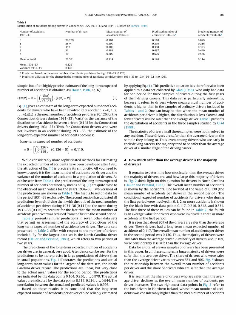
One of the first researchers who presented data on the distri-bution of accidents in a population of drivers was Forbes (1939),who in 1939 presented data on the distribution of accidents among29,531 drivers in the state of Connecticut for two three-year peri-ods: 1931–33 and 1934–36. Forbes states that the data were takenfrom a report of the Bureau of Public Roads. Table 1 reproducesthese data.
It is seen that most drivers were not involved in an accident inthe first three years. On the average, these drivers were involvedin 0.101 accidents in the second three years. 2874 drivers wereinvolved in one accident in the first three years. On the average,these drivers were involved in 0.199 accidents in the second threeyears. The mean number of accidents per driver among drivers whowere involved in 1, 2, 3 or 4 accidents during the first three yearswas substantially reduced in the second three years. Conversely,the mean number of accidents per driver increased from the firstto the second three years among drivers who were not involved inaccidents during the first three years.
These changes are an example of regression-to-the-mean. Therecorded number of accidents during the first three years is not anunbiased estimator of the long-term expected number of accidentsper driver, but is partly the result of random fluctuations around themean value. The relative contributions from random and system-atic variation in the number of accidents to the recorded numberof accidents per driver during the first three years can be deter-mined by examining the ratio of the mean to the variance. In general(Hauer, 1986):
Variation in the recorded number of accidents = Random variation
+ Systematic variation
It is generally assumed that random variation in the num-ber of accidents can be modelled statistically by means of thePoisson distribution (Fridstrøm et al., 1995). If variation in therecorded number of accidents was purely random, the varianceof the distribution of accidents among drivers would equal themean number of accidents per driver, because the variance equalsthe mean in a Poisson-distribution. In the population of driversin Connecticut during the period 1931–33, the mean number ofaccidents per driver was 0.126. The variance was 0.145. Hence,(0.126/0.145) × 100 = 86.9% of the variation in the recorded numberof accidents was random and [(0.145 − 0.126)/0.145] × 100 = 13.1%was systematic.
The systematic variation in the number of accidents, which isvariation in the long-term expected number of accidents per driver,is reflected in the differences in the mean number of accidents perdriver in the period 1934–36 for drivers who were involved in 0,1, 2, 3 or 4 accidents in the period 1931–33. Random variationis eliminated from the first to the second three-year period andonly systematic variation remains. Thus, the mean number of acci-dents per driver during the period 1934–36 reflects the long-term
expected number of accidents per driver.
The long-term expected number of accidents per driver can beestimated on the basis of knowledge of the mean and variance ofthe distribution of accidents between drivers in the first period. A
R. Elvik / Accident Analysis and Prevention 59 (2013) 301– 308 303
Table 1Distribution of accidents among drivers in Connecticut, USA, 1931–33 and 1934–36. Based on Forbes (1939).
a Prediction based on the mean number of accidents per driver during 1931–33 (b Prediction adjusted for the change in the mean number of accidents per driver
imple, but often highly precise estimate of the long-term expectedumber of accidents is obtained as (Hauer, 1986, Eq. 6):
(m|x) = x +[(
E(x)Var(x)
)· (E(x) − x)
](1)
q. (1) gives an estimate of the long-term expected number of acci-ents for drivers who have been involved in x accident (x = 0, 1, 2,
. ., n). E(x) is the mean number of accidents per driver (0.126 for theonnecticut drivers during 1931–33). Var(x) is the variance of theistribution of accidents between drivers (0.145 for the Connecticutrivers during 1931–33). Thus, for Connecticut drivers who wereot involved in an accident during 1931–33, the estimate of the
ong-term expected number of accidents becomes:
Long-term expected number of accidents
= 0 +[(
0.1260.145
)· (0.126 − 0)
]= 0.110.
While considerably more sophisticated methods for estimatinghe expected number of accidents have been developed after 1986,he attraction of Eq. (1) is precisely its simplicity. All you need tonow to apply it is the mean number of accidents per driver and theariance of the number of accidents in a population of drivers. Asan be seen from Table 1, the predictions of the long-term expectedumber of accidents obtained by means of Eq. (1) are quite close tohe observed mean values for the years 1934–36. Two versions ofhe predictions are shown in Table 1. The first is based on data forhe period 1931–33 exclusively. The second version has adjusted allredictions by multiplying them with the ratio of the mean numberf accidents per driver during 1934–36 (0.114) to the mean during931–33 (0.126) to account for the fact that the mean number ofccidents per driver was reduced from the first to the second period.
Table 2 presents similar predictions in seven other data setshat permit an assessment of the accuracy of predictions of theong-term expected number of accidents per driver. The data setsresented in Table 2 differ with respect to the number of drivers
ncluded. By far the largest data set is the North Carolina driverecord (Hauer and Persaud, 1983), which refers to two periods ofwo years.
The predictions of the long-term expected number of accidentser driver are, in general, very good. A tendency can be seen for theredictions to be more precise in large populations of drivers than
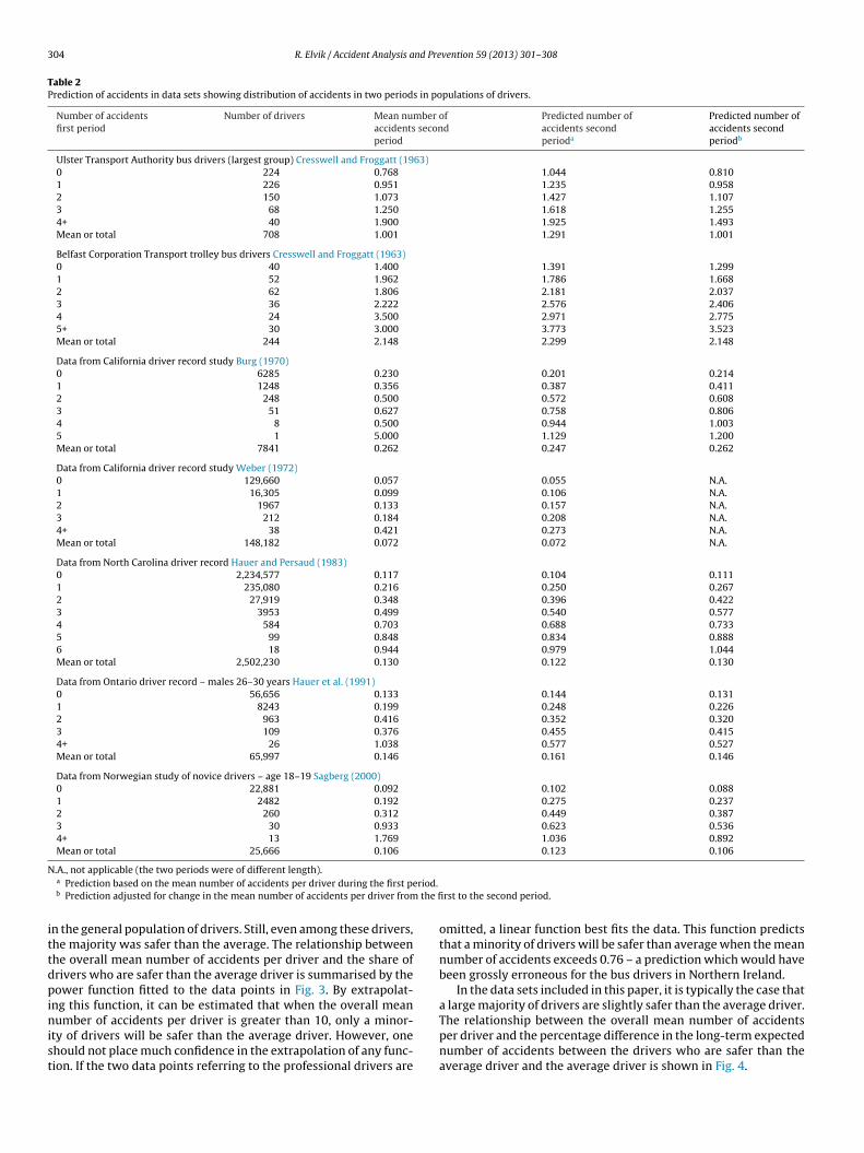
n small populations. Fig. 1 illustrates the predictions and actualong-term mean values for the largest of the data sets, the Northarolina driver record. The predictions are linear, but very closeo the actual mean values for the second period. The predictionsre indicated by the data points 0.104, 0.250, . . ., 0.979. The actual
alues are indicated by the data points 0.117, 0.216, . . ., 0.944. Theorrelation between the actual and predicted values is 0.996.
Based on these results, it is concluded that the long-termxpected number of accidents per driver can be reliably estimated
).931–33 to 1934–36 (0.114/0.126).
by applying Eq. (1). This predictive equation has therefore also beenapplied to a data set collected by Glad (1988), who only had datafor one period for three samples of drivers during the first yearsof their driving careers. This data set is particularly interesting,because it refers to drivers whose mean annual number of acci-dents is higher than in the samples of ordinary drivers included inTables 1 and 2. One can imagine that when the mean number ofaccidents per driver is higher, the distribution is less skewed andfewer drivers will be safer than the average driver. Table 3 presentsthe distribution of accidents in the three samples studied by Glad(1988).
The majority of drivers in all three samples were not involved inany accident. These drivers are safer than the average driver in thesample they belong to. Thus, even among drivers who are early intheir driving careers, the majority tend to be safer than the averagedriver at a similar stage of the driving career.
4. How much safer than the average driver is the majorityof drivers?
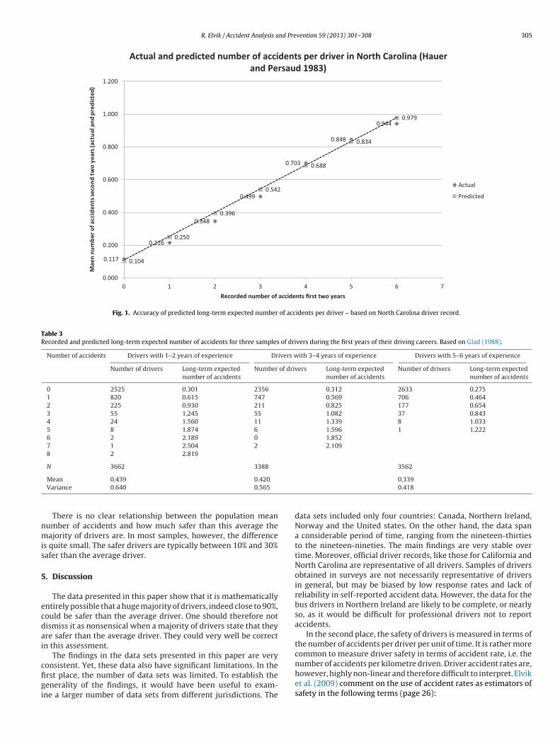
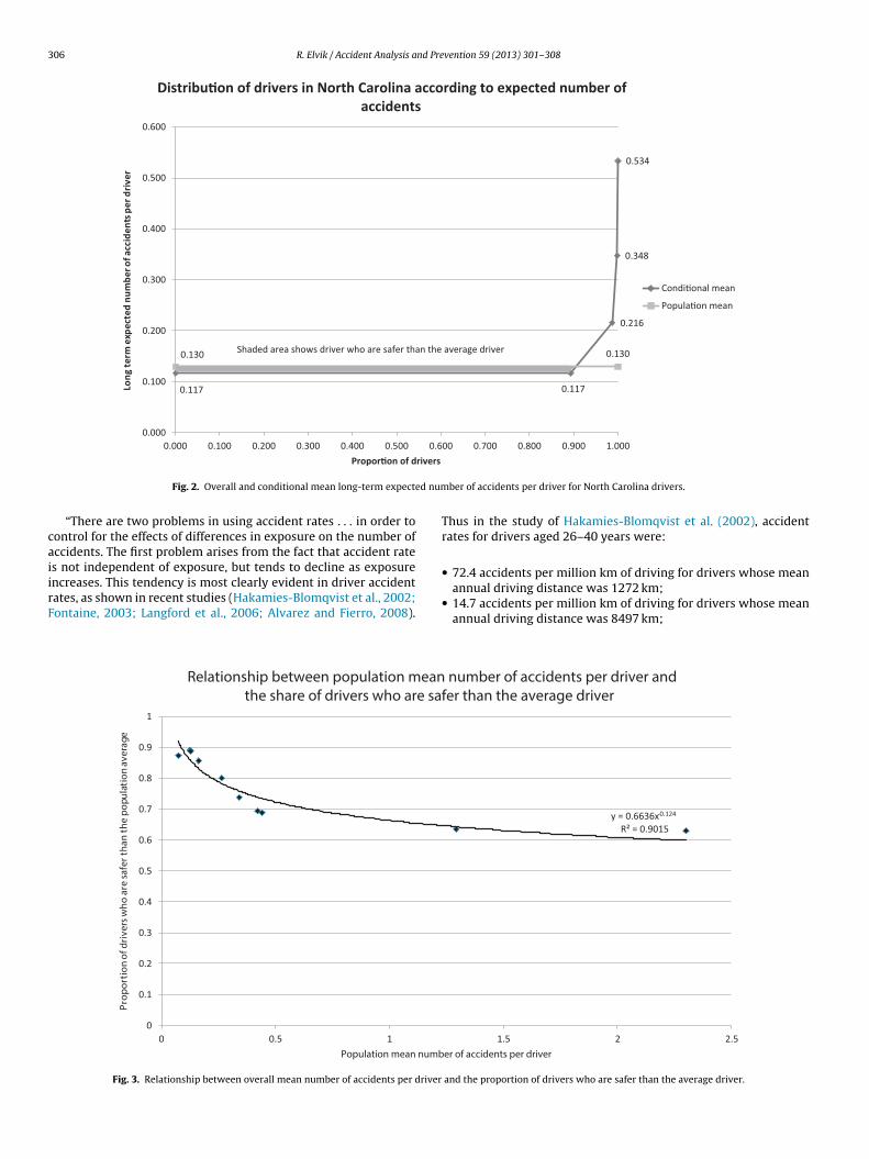
It remains to determine how much safer than the average driverthe majority of drivers are, and how large this majority of driversis. Fig. 2 sheds light on this question for drivers in North Carolina(Hauer and Persaud, 1983). The overall mean number of accidentsis shown by the horizontal line located at the value of 0.130 (themean number of accidents per driver in the second period). Theconditional expected number of accidents for drivers who duringthe first period were involved in 0, 1, 2, or more accidents is shownby the black line with data points 0.117, 0.216, 0.348, and 0.534.The first three of these values can be found in Table 2; the fourthis an average value for drivers who were involved in three or moreaccidents in the first period.
It is seen that about 90% of the drivers are safer than the averagedriver. These drivers had a long-term mean expected number ofaccidents of 0.117. The overall mean number of accidents per driverin the second period was 0.130. Thus, the majority of drivers were10% safer than the average driver. A minority of drivers, about 10%,were considerably less safe than the average driver.
Data for a total of eleven samples of drivers has been presentedin this paper. In all these samples, a huge majority of drivers weresafer than the average driver. The share of drivers who were saferthan the average driver varies between 63% and 90%. Fig. 3 showsthe relationship between the overall mean number of accidentsper driver and the share of drivers who are safer than the averagedriver.
It is seen that the share of drivers who are safer than the aver-
age driver declines as the overall mean number of accidents perdriver increases. The two rightmost data points in Fig. 3 refer tothe bus drivers in Northern Ireland, whose mean number of acci-dents was considerably higher than the mean number of accidents
304 R. Elvik / Accident Analysis and Prevention 59 (2013) 301– 308
Table 2Prediction of accidents in data sets showing distribution of accidents in two periods in populations of drivers.
Number of accidentsfirst period
Number of drivers Mean number ofaccidents secondperiod
Predicted number ofaccidents secondperioda
Predicted number ofaccidents secondperiodb
Ulster Transport Authority bus drivers (largest group) Cresswell and Froggatt (1963)0 224 0.768 1.044 0.8101 226 0.951 1.235 0.9582 150 1.073 1.427 1.1073 68 1.250 1.618 1.2554+ 40 1.900 1.925 1.493Mean or total 708 1.001 1.291 1.001
Belfast Corporation Transport trolley bus drivers Cresswell and Froggatt (1963)0 40 1.400 1.391 1.2991 52 1.962 1.786 1.6682 62 1.806 2.181 2.0373 36 2.222 2.576 2.4064 24 3.500 2.971 2.7755+ 30 3.000 3.773 3.523Mean or total 244 2.148 2.299 2.148
Data from California driver record study Burg (1970)0 6285 0.230 0.201 0.2141 1248 0.356 0.387 0.4112 248 0.500 0.572 0.6083 51 0.627 0.758 0.8064 8 0.500 0.944 1.0035 1 5.000 1.129 1.200Mean or total 7841 0.262 0.247 0.262
Data from California driver record study Weber (1972)0 129,660 0.057 0.055 N.A.1 16,305 0.099 0.106 N.A.2 1967 0.133 0.157 N.A.3 212 0.184 0.208 N.A.4+ 38 0.421 0.273 N.A.Mean or total 148,182 0.072 0.072 N.A.
Data from North Carolina driver record Hauer and Persaud (1983)0 2,234,577 0.117 0.104 0.1111 235,080 0.216 0.250 0.2672 27,919 0.348 0.396 0.4223 3953 0.499 0.540 0.5774 584 0.703 0.688 0.7335 99 0.848 0.834 0.8886 18 0.944 0.979 1.044Mean or total 2,502,230 0.130 0.122 0.130
Data from Ontario driver record – males 26–30 years Hauer et al. (1991)0 56,656 0.133 0.144 0.1311 8243 0.199 0.248 0.2262 963 0.416 0.352 0.3203 109 0.376 0.455 0.4154+ 26 1.038 0.577 0.527Mean or total 65,997 0.146 0.161 0.146
Data from Norwegian study of novice drivers – age 18–19 Sagberg (2000)0 22,881 0.092 0.102 0.0881 2482 0.192 0.275 0.2372 260 0.312 0.449 0.3873 30 0.933 0.623 0.5364+ 13 1.769 1.036 0.892Mean or total 25,666 0.106 0.123 0.106
Neriod.
the fi
ittdpinist
.A., not applicable (the two periods were of different length).a Prediction based on the mean number of accidents per driver during the first pb Prediction adjusted for change in the mean number of accidents per driver from
n the general population of drivers. Still, even among these drivers,he majority was safer than the average. The relationship betweenhe overall mean number of accidents per driver and the share ofrivers who are safer than the average driver is summarised by theower function fitted to the data points in Fig. 3. By extrapolat-
ng this function, it can be estimated that when the overall mean
umber of accidents per driver is greater than 10, only a minor-
ty of drivers will be safer than the average driver. However, onehould not place much confidence in the extrapolation of any func-ion. If the two data points referring to the professional drivers are
rst to the second period.
omitted, a linear function best fits the data. This function predictsthat a minority of drivers will be safer than average when the meannumber of accidents exceeds 0.76 – a prediction which would havebeen grossly erroneous for the bus drivers in Northern Ireland.
In the data sets included in this paper, it is typically the case thata large majority of drivers are slightly safer than the average driver.
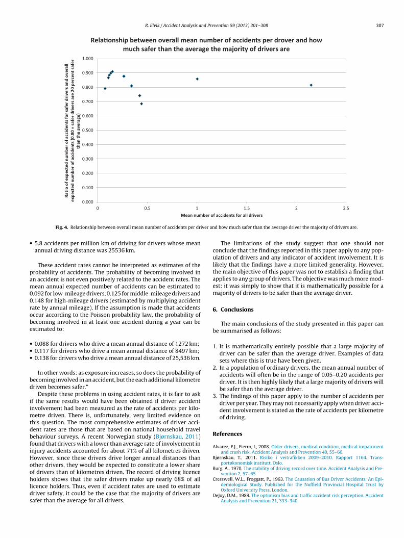
The relationship between the overall mean number of accidentsper driver and the percentage difference in the long-term expectednumber of accidents between the drivers who are safer than theaverage driver and the average driver is shown in Fig. 4.
R. Elvik / Accident Analysis and Prevention 59 (2013) 301– 308 305
0.117
0.216
0.348
0.499
0.703
0.848
0.944
0.104
0.250
0.396
0.542
0.688
0.834
0.979
0.000
0.200
0.400
0.600
0.800
1.000
1.200
0 1 2 3 4 5 6 7
)detciderpdnalautca(sraey
owt
dn ocesstnediccaforebmun
neaM
Recorded number of accidents first two years
Actual and predicted number of accidents per driver in North Carolina (Hauer and Persaud 1983)
Actual
Predicted
Fig. 1. Accuracy of predicted long-term expected number of accidents per driver – based on North Carolina driver record.
Table 3Recorded and predicted long-term expected number of accidents for three samples of drivers during the first years of their driving careers. Based on Glad (1988).
Number of accidents Drivers with 1–2 years of experience Drivers with 3–4 years of experience Drivers with 5–6 years of experience
Number of drivers Long-term expectednumber of accidents
Number of drivers Long-term expectednumber of accidents
Number of drivers Long-term expectednumber of accidents
There is no clear relationship between the population meanumber of accidents and how much safer than this average theajority of drivers are. In most samples, however, the difference
s quite small. The safer drivers are typically between 10% and 30%afer than the average driver.
. Discussion
The data presented in this paper show that it is mathematicallyntirely possible that a huge majority of drivers, indeed close to 90%,ould be safer than the average driver. One should therefore notismiss it as nonsensical when a majority of drivers state that theyre safer than the average driver. They could very well be correctn this assessment.
The findings in the data sets presented in this paper are very
onsistent. Yet, these data also have significant limitations. In therst place, the number of data sets was limited. To establish theenerality of the findings, it would have been useful to exam-ne a larger number of data sets from different jurisdictions. The
0.3390.418
data sets included only four countries: Canada, Northern Ireland,Norway and the United states. On the other hand, the data spana considerable period of time, ranging from the nineteen-thirtiesto the nineteen-nineties. The main findings are very stable overtime. Moreover, official driver records, like those for California andNorth Carolina are representative of all drivers. Samples of driversobtained in surveys are not necessarily representative of driversin general, but may be biased by low response rates and lack ofreliability in self-reported accident data. However, the data for thebus drivers in Northern Ireland are likely to be complete, or nearlyso, as it would be difficult for professional drivers not to reportaccidents.
In the second place, the safety of drivers is measured in terms ofthe number of accidents per driver per unit of time. It is rather morecommon to measure driver safety in terms of accident rate, i.e. the
number of accidents per kilometre driven. Driver accident rates are,however, highly non-linear and therefore difficult to interpret. Elviket al. (2009) comment on the use of accident rates as estimators ofsafety in the following terms (page 26):
306 R. Elvik / Accident Analysis and Prevention 59 (2013) 301– 308
Distribu�on of drivers in North Carolina according to expected number of accidents
Condi�onal mean
Popula�on mean
Shaded area shows driver who are safer than the average driver
ed num
caiirF
Propor�on of d
Fig. 2. Overall and conditional mean long-term expect
“There are two problems in using accident rates . . . in order toontrol for the effects of differences in exposure on the number ofccidents. The first problem arises from the fact that accident rate
s not independent of exposure, but tends to decline as exposurencreases. This tendency is most clearly evident in driver accidentates, as shown in recent studies (Hakamies-Blomqvist et al., 2002;ontaine, 2003; Langford et al., 2006; Alvarez and Fierro, 2008).
0
0.1
0.2
0.3
0.4
0.5
0.6
0.7
0.8
0.9
1
0 0.5 1
egarevanoitalup op
e htnah trefas
erao h
wsre virdfonoitroporP
Population mean numb
Relationship between population meanthe share of drivers who are sa
Fig. 3. Relationship between overall mean number of accidents per driver
ber of accidents per driver for North Carolina drivers.
Thus in the study of Hakamies-Blomqvist et al. (2002), accidentrates for drivers aged 26–40 years were:
• 72.4 accidents per million km of driving for drivers whose meanannual driving distance was 1272 km;
• 14.7 accidents per million km of driving for drivers whose meanannual driving distance was 8497 km;
y = 0.6636x-0.124
R² = 0.9015
1.5 2 2.5er of accidents per driver
number of accidents per driver and fer than the average driver
and the proportion of drivers who are safer than the average driver.
R. Elvik / Accident Analysis and Prevention 59 (2013) 301– 308 307
0.000
0.100
0.200
0.300
0.400
0.500
0.600
0.700
0.800
0.900
1.000
0 0.5 1 1.5 2 2.5
llarevodnasrevirdrefasrofstnediccaforeb
mundetcepxefo
oitaRex
pect
ed n
umbe
r of a
ccid
ents
(0.8
0 =
safe
r driv
ers a
re 2
0 pe
rcen
t saf
er
than
the
aver
age)
ber o
Rela�onship between overall mean number of accidents per drover and how much safer than the average the majority of drivers are
iver an
•
pam00robe
•••
bd
iimtdbfiHoohlds
Mean num
Fig. 4. Relationship between overall mean number of accidents per dr
5.8 accidents per million km of driving for drivers whose meanannual driving distance was 25536 km.
These accident rates cannot be interpreted as estimates of therobability of accidents. The probability of becoming involved inn accident is not even positively related to the accident rates. Theean annual expected number of accidents can be estimated to
.092 for low-mileage drivers, 0.125 for middle-mileage drivers and
.148 for high-mileage drivers (estimated by multiplying accidentate by annual mileage). If the assumption is made that accidentsccur according to the Poisson probability law, the probability ofecoming involved in at least one accident during a year can bestimated to:
0.088 for drivers who drive a mean annual distance of 1272 km;0.117 for drivers who drive a mean annual distance of 8497 km;0.138 for drivers who drive a mean annual distance of 25,536 km.
In other words: as exposure increases, so does the probability ofecoming involved in an accident, but the each additional kilometreriven becomes safer.”
Despite these problems in using accident rates, it is fair to askf the same results would have been obtained if driver accidentnvolvement had been measured as the rate of accidents per kilo-
etre driven. There is, unfortunately, very limited evidence onhis question. The most comprehensive estimates of driver acci-ent rates are those that are based on national household travelehaviour surveys. A recent Norwegian study (Bjørnskau, 2011)ound that drivers with a lower than average rate of involvement innjury accidents accounted for about 71% of all kilometres driven.owever, since these drivers drive longer annual distances thanther drivers, they would be expected to constitute a lower sharef drivers than of kilometres driven. The record of driving licence
olders shows that the safer drivers make up nearly 68% of all
icence holders. Thus, even if accident rates are used to estimateriver safety, it could be the case that the majority of drivers areafer than the average for all drivers.
f accidents for all drivers
d how much safer than the average driver the majority of drivers are.
The limitations of the study suggest that one should notconclude that the findings reported in this paper apply to any pop-ulation of drivers and any indicator of accident involvement. It islikely that the findings have a more limited generality. However,the main objective of this paper was not to establish a finding thatapplies to any group of drivers. The objective was much more mod-est: it was simply to show that it is mathematically possible for amajority of drivers to be safer than the average driver.
6. Conclusions
The main conclusions of the study presented in this paper canbe summarised as follows:
1. It is mathematically entirely possible that a large majority ofdriver can be safer than the average driver. Examples of datasets where this is true have been given.
2. In a population of ordinary drivers, the mean annual number ofaccidents will often be in the range of 0.05–0.20 accidents perdriver. It is then highly likely that a large majority of drivers willbe safer than the average driver.
3. The findings of this paper apply to the number of accidents perdriver per year. They may not necessarily apply when driver acci-dent involvement is stated as the rate of accidents per kilometreof driving.
References
Alvarez, F.J., Fierro, I., 2008. Older drivers, medical condition, medical impairmentand crash risk. Accident Analysis and Prevention 40, 55–60.
Bjørnskau, T., 2011. Risiko i veitrafikken 2009–2010. Rapport 1164. Trans-portøkonomisk institutt, Oslo.
Burg, A., 1970. The stability of driving record over time. Accident Analysis and Pre-vention 2, 57–65.
Cresswell, W.L., Froggatt, P., 1963. The Causation of Bus Driver Accidents. An Epi-demiological Study. Published for the Nuffield Provincial Hospital Trust byOxford University Press, London.
DeJoy, D.M., 1989. The optimism bias and traffic accident risk perception. AccidentAnalysis and Prevention 21, 333–340.
Svenson, O., Fischhoff, B., MacGregor, D., 1985. Perceived driving safety and seatbelt
08 R. Elvik / Accident Analysis a
lvik, R., Erke, A., Christensen, P., 2009. Elementary units of exposure. TransportationResearch Record 2103, 25–31.
ontaine, H., 2003. Driver age and road accidents. What is the risk for seniors?Recherche Transports Sécurité 79, 107–120.
orbes, T.W., 1939. The normal automobile driver as a traffic problem. Journal ofGeneral Psychology 20, 471–474.
ridstrøm, L., Ifver, J., Ingebrigtsen, S., Kulmala, R., Krogsgård Thomsen, L., 1995.Measuring the contribution of randomness, exposure, weather, and daylight tothe variation in road accident counts. Accident Analysis and Prevention 27, 1–20.
lad, A., 1988. Fase 2 i føreropplæringen. Effekt på ulykkesrisikoen. Rapport 0015.Transportøkonomisk institutt, Oslo.
akamies-Blomqvist, L., Raitanen, T., O’Neill, D., 2002. Driver ageing does not causehigher accident rates per km. Transportation Research Part F 5, 271–274.
arré, N., Sibley, C.G., 2007. Explicit and implicit self-enhancement biases in driversand their relationship to driving violations and crash-risk optimism. AccidentAnalysis and Prevention 39, 1155–1161.
auer, E., 1986. On the estimation of the expected number of accidents. AccidentAnalysis and Prevention 18, 1–12.
auer, E., 1997. Observational Before–After Studies in Road Safety. Estimating theEffect of Highway and Traffic Engineering Measures on Road Safety. PergamonPress, Oxford.
vention 59 (2013) 301– 308
Hauer, E., Persaud, B., 1983. Common bias in before-and-after accident comparisonsand its elimination. Transportation Research Record 905, 164–174.
Hauer, E., Persaud, B.N., Smiley, A., Duncan, D., 1991. Estimating the acci-dent potential of an Ontario driver. Accident Analysis and Prevention 23,133–152.
Holland, C.A., 1993. Self-bias in older drivers’ judgments of accident likelihood.Accident Analysis and Prevention 25, 431–441.
Langford, J., Methorst, R., Hakamies-Blomqvist, L., 2006. Older drivers do not havea high crash risk – a replication of low mileage bias. Accident Analysis andPrevention 38, 574–578.
Sagberg, F., 2000. Evaluering av 16-årsgrense for øvelseskjøring med personbil.Ulykkesrisiko etter førerprøven. Rapport 498. Transportøkonomisk institutt,Oslo.
Svenson, O., 1981. Are we all less risky and more skillful than our fellow drivers?Acta Psychologica 47, 143–148.
usage. Accident Analysis and Prevention 17, 119–133.Weber, D.C., 1972. An analysis of the California driver record study in the
context of a classical accident model. Accident Analysis and Prevention 4,109–116.