Can Violence Harm Cooperation? Experimental Evidence · Can Violence Harm Cooperation? Experimental...

Can Violence Harm Cooperation? Experimental Evidence

Giacomo De Luca∗, Petros G. Sekeris†, and Dominic E. Spengler‡

Abstract

While folk theorems for dynamic renewable common pool resource games sustain cooperation at equi-

librium, the possibility of appropriating violently the resource can destroy the incentives to cooperate,

because of the expectation of conflict when resources are sufficiently depleted. This paper provides ex-

perimental evidence that individuals behave according to the theoretical predictions. For high stocks of

resources, when conflict is a costly activity, participants cooperate less than in the control group, and play

non-cooperatively with higher frequency. This comes as a consequence of the anticipation that, when

resources run low, the conflict option is used by a large share of participants.

Keywords: Experiment, Dynamic Game, Cooperation

JEL classification: C72; C73; C91; D74

1 Introduction

The depletion of the world’s renewable natural resources has become increasingly concerning and is re-

flected in the warnings of the scientific community (Homer Dixon 1999, Stern 2007). When such resources

are commonly managed, they are prone to the tragedy of the commons problem, i.e. over-extraction resulting

from inherent externality problems (Hardin 1968). The management of these resources is best described in

a formal dynamic setting, which allows to capture the regenerative nature of resources through time. In a∗University of York. Contact e-mail: [email protected]†University of Portsmouth. Contact e-mail: [email protected]‡University of York. Contact e-mail: [email protected]

1

dynamic setting, cooperation on the efficient extraction of a renewable resource can be sustained among re-

source users by the threat of reverting to noncooperation in case of noncompliance to some agreed behaviour

(Cave 1987, Dutta 1995, Sorger 2005, Dutta and Radner 2009).

More recently, the game theoretic predictions on the management of the commons have received exten-

sive attention by experimental economists. The early experimental literature focused on testing the equilib-

rium behavior generated by repeated games (Palfrey and Rosenthal 1994, Dal Bo 2005), or finite dynamic

games (Herr et al. 1997). In general, findings tend to concur with the theoretical predictions, suggesting that

free riding and therefore inefficiencies do arise, and that dynamics help fostering the cooperative equilib-

rium through reputation mechanisms and the existence of latent punishment schemes.1 Exploring whether

cooperation can be sustained in dynamic games of resource exploitation is a more challenging question that

has only been tackled recently (Dal Bo and Frechette 2014). Since the cooperative extraction level can be

sustained with several different subgame perfect punishments, experimental economists need to limit their

experimental tests to a (some) specific strategie(s). Vespa (2014) shows that individuals tend to cooperate in

a dynamic renewable common pool resource (CPR) game if given the possibility to “cooperate” or “defect”

to the non-cooperative Markovian strategy. Yet such cooperation is jeopardized when participants are of-

fered the choice of a “highly profitable” deviation. These findings therefore seem to suggest that individuals

do cooperate under the threat of some punishment strategies.

The punishment strategies described above rely on the dynamic nature of the game. As a consequence,

the picture changes if players are given the possibility to alter the nature of the game via their actions. Sekeris

(2014) demonstrates that in a dynamic renewable CPR game, where individuals are given the choice to revert

to violence at any point in time so as to claim ownership of the common resource, the efficient solution may

not be sustainable at equilibrium. This follows from the players’ incentives to violently appropriate the CPR

when the resource becomes scarce, which renders the non-cooperative punishments necessary to support

cooperation not subgame perfect, and therefore invalidates the logic of Folk theorems. Given the important

consequences that such reasoning may have with regards to the conservation of resources that are vital for

sustaining human life, such as fresh water, land and fossil fuels, it is crucial to inquire whether individuals

do act as rational theory predicts. In this paper we therefore experimentally investigate whether in settings

comparable to Sekeris (2014) participants act as predicted by the theory.

1Scholars have also demonstrated a tendency of participants to use costly punishments against non-cooperators, even that leaves

them materially worse-off (Fehr and Gaechter 2000, Casari and Plott, 2003).

2

A burgeoning experimental literature on conflicts has emerged lately.2 While the initial contributions

subjected to experimental validation static theories of conflict, the dynamic considerations we are focusing

on have equally received attention by scholars more recently (Abbink and de Haan 2014, Lacomba et al.

2014, McBride and Skaperdas 2014). Yet, whereas these contributions perceive conflict as an appropriation

of private goods and/or production potential, our approach conceives the status quo as a CPR game. Coop-

eration in experimental conflict settings has equally received some attention, albeit the focus of the existing

literature has been on alliance formation and group fighting as opposed to cooperation in the production pro-

cess (Abbink et al. 2010, Ke et al. 2015, Herbst et al. forthcoming). Moreover, to conform to the dynamic

theory that we are testing, we design a conflict experiment replicating an infinite-horizon game as in Vespa

(2014).

In this paper we consider a CPR where costly appropriation of the resources is allowed for, and we

experimentally explore whether the costliness of conflict influences the incentives to cooperate. To that end,

we develop a simplified version of the model in Sekeris (2014), which allows us to derive clear predictions

with regards to the players’ optimal strategies. In the presence of prohibitively costly appropriation, the

theory predicts that cooperation can be sustained at equilibrium. If the cost of appropriation decreases

as resources become scarcer, results change dramatically: individuals stop cooperating by opting for non-

cooperation in the early stages of the game, and eventually resort to costly appropriation. Notice that this

apparently restrictive assumption is an endogenous feature in Sekeris (2014) where conflict is modeled as a

standard contest success function. In order to keep the model simple and tractable, we decided to impose

this feature as an assumption in this paper.

To experimentally evaluate the applicability of this theory, we design two treatments and compare coop-

eration rates across them. Each treatment involves 58 participants, for a combined total of 116 students from

the University of York (UK). In both treatments participants are randomly matched into pairs and then called

to decide the amount of ‘points’ to extract from a pool of points at each ‘round’ of the game, and given a pre-

defined regeneration rate of the CPR. In the first treatment, which we label the ‘chance’ treatment, during

each ‘round’ participants are given the possibility to extract either a ‘low’ level of points corresponding to the

theoretical prediction of a cooperative extraction, or a ‘high’ level of points corresponding to the theoretical

prediction of a non-cooperative (Markov-perfect) extraction. In addition to ‘low’ and ‘high’, participants are

given the choice of opting for resource appropriation, denoted by ‘chance’, whereby the CPR is split equally

2see Dechenaux et al. (2014) for a recent review of the literature.

3

between the two paired individuals, at some cost which is increasing in the stock of the CPR.3 If at some

time period chance is played, the optimal extraction path is imposed on participants from the subsequent

time period and thereafter.

The second treatment named ‘costly chance’ is identical to the ‘chance’ treatment, except for the cost

of opting for resource appropriation, which is substantially increased to make it theoretically suboptimal.

In other words, we offer participants the same three options as in the ‘chance’ treatment (i.e. low, high

extraction rates and chance), but if chance is chosen 60% of the CPR is destroyed, thus making that choice

suboptimal for any level of resources.

To emulate the infinite horizon environment required for folk theorems to be applicable, we follow the

methodology in Vespa (2014) which was first introduced by Roth and Murnighan (1978) and later applied

by Cabral et al. (2011). The technique introduces an uncertain time horizon by allowing the software to

terminate the game at any ‘time period’ with some predetermined probability. This practice - which in theory

is equivalent to an infinite time horizon if individuals are risk neutral - has been shown not to be innocuous in

practice (Dal bo 2005, Frechette and Yuksel 2014). Since both our control and treatment groups are subject

to the same random termination rule, however, the validity of our experiment is not jeopardized.

Our experimental findings support our theoretical predictions. In the initial rounds of the game where

conflict is unlikely to have been selected in either treatment, in the chance treatment the level of cooperation

is lower compared to the costly-chance treatment, and non-cooperation is higher. Hence, the expectation

of a higher likelihood of chance being played in later stages of the game in the chance treatment reduces

cooperation in favour of non-cooperation in the early stages of the game. Restricting the analysis to the early

rounds of the game (or alternatively to high levels of CPR) confirms that participants tend to non-cooperate

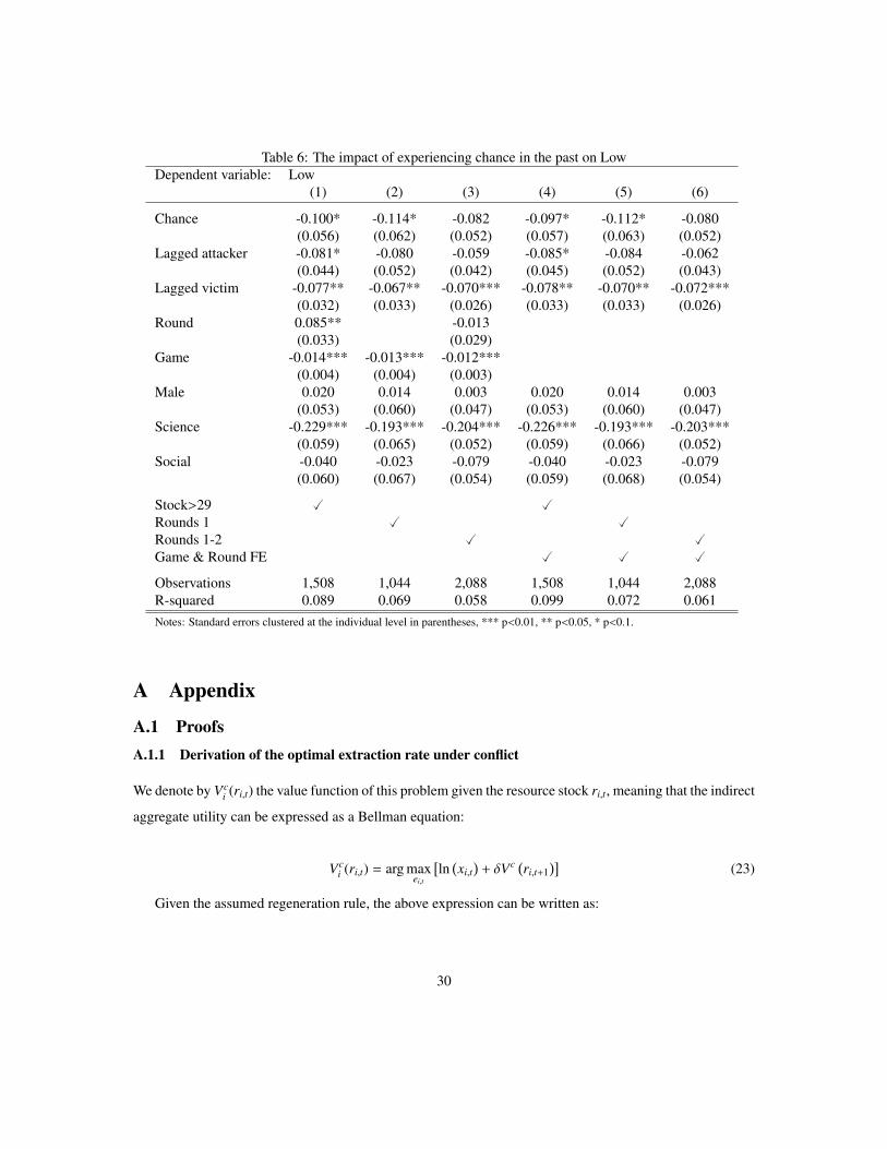
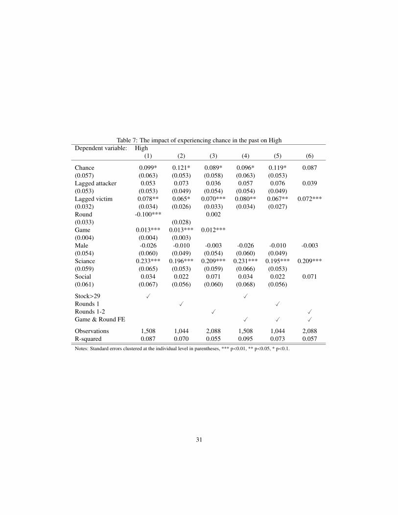
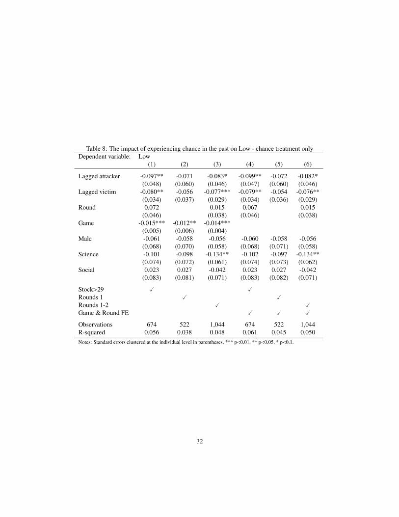
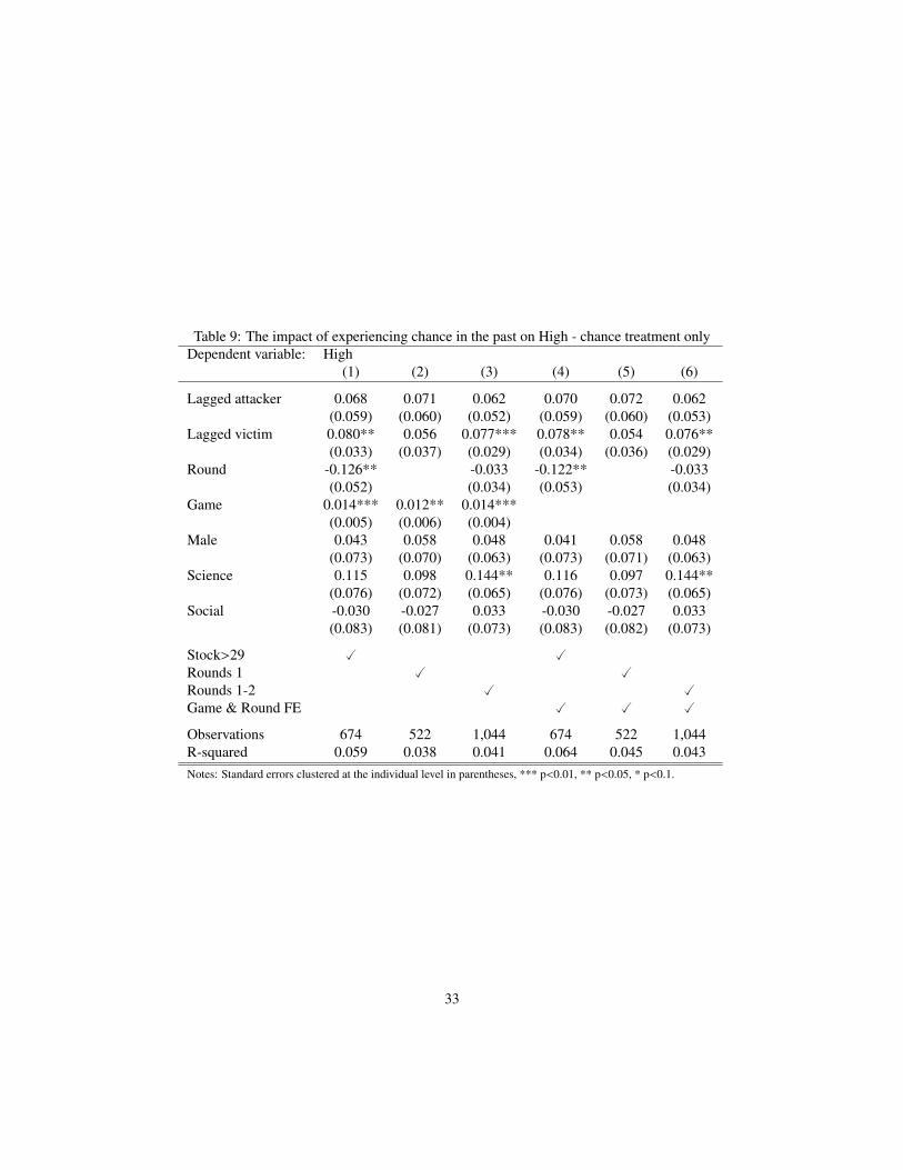
more in expectation of chance being potentially chosen in subsequent rounds. Moreover, we supplement

the analysis with a test supporting the theoretical mechanism underlying the participants’ behaviour. We

demonstrate that participants that experienced violence in a specific game are more likely to behave accord-

ing to predictions in the subsequent game, thus providing evidence that a higher expectation of chance being

played incentivizes the participants to substitute cooperation by non-cooperation. Lastly, we track individual

paths of play by participants, and we find that in 24% of the games being played in the chance treatment, par-

ticipants behave according to the theoretical predictions. In the costly-chance treatment, however, no single

3We deliberately chose a neutral tag to denote the conflict action in our experiment to avoid any framing bias. In particular,

had we named our resource appropriation ‘conflict’ or ‘violence’, changes in cooperation rates across treatments may have been the

consequence of different moral/ethical values among participants.

4

participant made these same choices. This constitutes compelling evidence that our experimental findings

are indeed driven by individual participants behaving as predicted by the theory.

In the following section we lay out the theoretical model, in Section 3 we describe the experimental

design, in Section 4 we present our experimental results, and lastly Section 5 concludes.

2 Theory

2.1 The setting

We consider a dynamic common pool resource game featuring a renewable resource, rt, initially owned

commonly by two players labeled 1 and 2. Time is discrete and denoted by t = {0, 1 . . .∞}. At any time

period t the two players make a conflict decision, (w1,t,w2,t), with wi,t = v if player i opts for violence, and

wi,t = p, otherwise. If either or both players opt for violence, conflict ensues. If conflict does not occur, in

a second stage the two players simultaneously decide the amount of resources to extract from the common

pool of resource, (e1,t, e2,t), and the game moves to the next time period. If conflict occurs, part of the

resources get destroyed and the remaining stock gets shared equally among the players forever after, thus

making conflict an absorbing state. The players then choose the amount of resources to extract from their -

now - private stock of resources, before the game moves to the next time period.

The initial resource endowment is given by r0 and the resource regenerates at some linear rate γ. Players

costlessly invest effort in resource-use, so that player i’s appropriation effort of renewable resources in time

t is denoted by ei,t, with ei,t ∈ [0, e], e > r0.

Conflict

In case of conflict in time τ the resources’ resilience is described by function φ(rτ), with φ(rτ)′

> 0 and

player i’s instantaneous consumption for any t ≥ τ is given by xi,t such that:

xi,t = ei,tri,t (1)

The law of motion of resources is given by:

rt+1 = (1 + γ)(ri,t − xi,t) (2)

5

The instantaneous utility of any player i in time t is given by:

ui,t = ln(xi,t) (3)

And the discounted life-time utility of player i in time period τ thus equals:

Uci (ri,τ) =

∞∑t=τ

δt−τ ln(xi,t

(ri,t

))(4)

where δ designates the discount rate, c denotes the conflict scenario, and ri,τ = φ(rτ)xτ/2.

No conflict

If conflict does not occur in time period t or at any earlier time period, player i’s instantaneous consump-

tion equals

xi,t =

ei,trt if e1,t + e2,t ≤ rt

ei,t

e1,t+e2,trt otherwise

(5)

The law of motion of resources is given by:

rt+1 = (1 + γ)(rt − x1,t − x2,t) (6)

And the discounted life-time utility of player i in time period t equals:

Ui,t = ln(xi,t) + δUi,t+1(rt+1) (7)

We denote a strategy for player i by (wi, ei) = {wi,t, ei,t}∞t=0. Our equilibrium concept is the subgame

perfect Nash equilibrium in dominant strategies.4

2.2 Equilibrium analysis

2.2.1 Preliminaries

The conflict subgame

Since conflict is an absorbing state, we begin by solving the subgame where either or both players chose

v. If in time period τ, (w1,τ,w2,τ) , (p, p), and conflict has not occurred for some t < τ, conflict takes place

4Focusing on dominant strategies allows us to rule out equilibria in (weakly) dominated strategies which - as will become clearer

below - are highly unrealistic.

6

in time τ. In Appendix A.1.1 we show that it is optimal for player i to extract a constant share of the available

stock of resources, so that at optimality ei,t = sci ri,t, with sc

i = 1 − δ.

Accordingly, along the optimal consumption path Expression (4) can be written as:

Vviolencei (rτ) =

11 − δ

ln((1 − δ)

φ(rτ)rτ2

)+

δ

(1 − δ)2 ln((1 + γ)δ) (8)

Eternal cooperation

A second building block of the equilibrium analysis is the ‘cooperative path’ whereby extractive effi-

ciency is achieved. Under this scenario both players choose extraction rates that internalize the negative

externality of resource depletion on the opponent. Stated otherwise, the ‘cooperative path’ is the central

planner solution which reads as:

maxe1,e2

∑i=1,2

∞∑t=0

δt ln(xi,t) (9)

s.t. (1) and (2)

We denote the players’ associated extraction rates by superscript l, i.e. ‘low’ extraction rates, and in the

remainder of the paper refer to such actions as ‘low’ actions. The solution to this problem, the details of

which can be found in Appendix A.1.2, is such that:

eli,t =

1 − δ2

rt i = {1, 2} (10)

Denoting by sl the (constant) optimal extraction share of either player at any time period t, we have

sl = (1−δ)/2. Accordingly, the cooperative strategy is given by the pair of vectors{wl

i, eli

}=

{p, slrt

}∞t=0

. The

proportion of the stock of resources which is preserved from one period to another therefore equals δ(1+γ).5

The discounted expected utility of both players following the cooperative strategy forever can be shown

to equal:

V li,t =

11 − δ

[ln

((1 − δ)rt

2

)+

δ

1 − δln(δ(1 + γ))

](11)

Eternal non-cooperation

We next derive the non-cooperative extraction path of this dynamic game. We denote the associated

strategies by h, i.e. ‘high’ extraction rates, and for the remainder of the paper we refer to these actions as

5Notice that the resource is dynamically depleted if (1 + γ)δ < 1⇔ γ < 1−δδ . For the problem to be salient, in the remainder of the

article we assume that this condition is satisfied.

7

‘high’ actions. In time period t the maximization problem for player i therefore reads as follows:

maxei

∞∑t=0

δt ln(xi,t) (12)

s.t. (1) and (2)

After optimizing, we obtain the high extraction levels:

ehi,t =

1 − δ2 − δ

rt i = {1, 2} (13)

Denoting by sh the (constant) optimal extraction share of either player at any time period t, we have

sh = (1 − δ)/(2 − δ). Accordingly, the non-cooperative strategy is defined by the pair of vectors{wh

i , ehi

}={

p, shrt}∞t=0

.

This enables us to compute the discounted expected utility of players following their non-cooperative

strategy:

Vhi,t −

11 − δ

[ln

((1 − δ)rt

2 − δ

)+

δ

1 − δln

(δ(1 + γ)

2 − δ

)](14)

2.2.2 Equilibrium with costly conflict

We first consider the game’s equilibria if conflict is highly damaging. More specifically, we assume that the

resilience function is defined by φ(rt) = φ, with φ ≤ 40.

Our next step consists in demonstrating that with such costly conflict technology, neither player finds

it optimal to opt for violence along the equilibrium path. To establish that, we simply demonstrate that

the non-cooperative strategy strictly dominates the conflict one by showing that the following inequality is

verified for the conflict technology considered:

Vci (rt) < Vh

i (rt) (15)

Replacing for the appropriate values and simplifying yields:

(1 − δ) ln (φ/2) + ln(2 − δ) < 0 (16)

And this inequality is always satisfied for φ ≤ 0.4 and for any δ.

We can now deduce that since both players following their non-cooperative strategies is a Markov perfect

equilibrium, it is necessarily a SPE of the game as well.

8

Our last step aims at establishing the conditions making also the cooperative strategies a SPE. The co-

operative strategy yields - by construction - a Pareto-dominant situation, and given the assumed symmetry

it equally yields a higher discounted expected intertemporal utility for each player than any alternative equi-

librium strategy for any given starting stock of resources. A strategy whereby players implement ‘low’

irrespective of the opponent’s action cannot be an equilibrium strategy, however, since the instantaneous

utility of deviating from the ‘low’ extraction rate is higher than the instantaneous utility of ‘low’. To sustain

cooperation, therefore, punishment strategies should be considered. A widespread strategy that supports the

cooperative extraction path as a SPE, is the Grim-trigger strategy, whereby any deviation from the ‘low’ ac-

tion by either player implies that both players revert to the non-cooperative SPE forever after. One interesting

route is therefore to derive the conditions that induce play of the cooperative path in equilibrium.

For cooperation to be sustained as a SPE it is sufficient that the following condition be satisfied:

ln(edev

i,t (elj,t)

)+ δVh

i

((rt − edev

i,t (elj,t) − el

j,t)(1 + γ))< V l

i (rt) (17)

where the dev superscript designates the “deviation” best response of player i to any extraction rate of player

j. In the above expression, since we are inspecting the condition for the cooperative path of play to be an

equilibrium, player i considers the deviation best response in time period t given player j’s ‘low’ extraction

level in time period t, and given the reversion to the non-cooperative SPE in period t + 1 (i.e. Grim-trigger

strategy).

It is shown in Appendix A.1.3 that, after replacing for the appropriate terms, this expression can be

written as:

δ ln(2 − δ) > (1 − δ) ln(1 + δ) (18)

which is true for any δ > 1/2. We can therefore state the following result:

Proposition 1. In a renewable resource exploitation game where conflict is costly, ‘low’ extraction of re-

sources is supported as a subgame perfect equilibrium by a Grim-trigger strategy of reversion to the non-

cooperative subgame perfect Nash strategy for any δ > 1/2.

While this is not the only punishment supporting ‘low’ extraction rates, it is a particularly convenient

punishment for an experimental application.6

6In particular, the strategy of mutual full exhaustion of the resource is subgame perfect and constitutes the harshest possible punish-

ment supporting the cooperative equilibrium for any (see Vespa 2014 and Sekeris 2014).

9

2.2.3 Equilibrium with varying cost of conflict

We now consider the game’s equilibria when the resources’ resilience φ(rt) is a function of the stock of

resources such that φ(rt) ∈ [0, 1], φ(rt)′

≤ 0, and ∃ ¯r > r > 0, whereby φ(r) = 1,∀r ≤ r and φ(r) = 0,∀r ≥ ¯r.

The function φ(rt) is continuous on the interval ]r, ¯r[.7

To understand how this conflict technology affects the game’s equilibria, we proceed in two steps. We

first demonstrate that playing ‘low’ eternally is not achievable because, through the dynamic depletion of the

resource, the game reaches a point where both players prefer deviating from ‘low’ to conflict. In a second

step, we demonstrate that playing ‘low’ in the short run alone is not implementable either.

To demonstrate that ‘low’ cannot be played forever at equilibrium, it is sufficient to establish that Inequal-

ity (18) is violated when the stock of resources falls below some threshold. For any rt+1 ≤ r, φ(rt+1) = 1

and Inequality (18) is violated for any value of δ. For any rt+1 ≥ ¯r, φ(rt+1) = 0, and the inequality is then

satisfied for any value of δ. Moreover, since φ(rt) is continuously defined on ]r, ¯r[, there exists a r ∈ [r, ¯r]

such that the inequality is violated for any rt+1 < r.

Having shown that ‘low’ cannot be sustained forever, we now demonstrate that ‘low’ is not sustainable in

the short run either and that the game’s unique subgame perfect equilibrium involves playing ‘high’ for high

stocks of resources, and conflict for low stocks of resources. To establish this, we exploit the previous result

according to which ‘low’ is not sustainable forever, together with the fact that for low levels of resources,

violence is better than the discounted expected utility of playing ‘high’ forever. The latter result is proven

by establishing that there exist values of rt, which satisfy the following inequality:

Vci (rt) > Vh

i (rt) (19)

Replacing for the appropriate values and simplifying yields:

(1 − δ) ln (φ(rt)/2) + ln(2 − δ) > 0 (20)

Replacing rt by r implies that the condition is satisfied for any δ.

7Notice that this set of simplifying assumptions about the conflict technology is meant to produce numerical results that can easily

be mapped in the lab, while also capturing the essence of Sekeris (2014) where the players’ armaments and therefore the associated

damage to the resource are endogenous. Indeed, no such - seemingly extreme - assumption on the conflict technology would be required

for our results to hold in a more elaborate model with endogenous armaments and a Contest Success function conflict technology. The

economic intuition for why abundant resources are less resilient to conflict is that in such instances the fight over the control of the

resources will be fiercer, thereby resulting in higher damage to the contested pie.

10

Defining by r the maximal value of resources satisfying inequality (20), we show that for any resources

rt > r players will play ‘high’. Assume that in period τ we expect conflict to be the preferred option if both

players expect each other to play ‘low’. Then in t = τ − 1, should one’s opponent play ‘low’, it is optimal

to play the deviation best response. Hence, as both players follow the same reasoning, in t = τ − 1 they will

both play ‘high’. This mutual non-cooperation is due to the fact that in time τ players have no punishment

scheme to support ‘low’. Applying the argument backwardly implies that players never play ‘low’, which

leads to the following proposition.

Proposition 2. In a renewable resource exploitation game where resources are increasingly resilient to

conflict when they are scarcer, the unique equilibrium is such that players choose ‘high’ if r > r and they

declare conflict if r ≤ r.

Combining the results of Propositions 1 and 2, we can enunciate the following corollary which will be

tested in the experimental section of the paper:

Corollary 1. In a renewable resource exploitation game where resources can be violently appropriated

at some cost, replacing a highly costly conflict technology by a technology making resources increasingly

resilient to conflict when resources are scarcer,

1. ‘low’ is substituted by ‘high’ when resources are sufficiently abundant.

2. Conflict is chosen when the resources are sufficiently depleted.

3 Experimental design

The theory developed in the previous section establishes two results. First, playing ‘low’ forever may be sup-

ported as a subgame perfect equilibrium of the game provided the conflict technology is sufficiently costly.

Second, when resources’ resilience to conflict increases with scarcity, the unique equilibrium involves play-

ers playing ‘high’ when the stock of resources is large, and opting for conflict when the stock of resources

drops below some threshold level. We now proceed to the experimental validation of the theory.

3.1 Parametrization

For the experimental game, we fix the parameters of the model such that (i) cooperation is supported as a SPE

in the costly-conflict version of the game, and (ii) conflict is the players’ prefered option when resources are

11

sufficiently depleted in the version of the game where resources’ resilience to conflict increases with scarcity,

therefore verifying Proposition 2.

For (i) to hold we require that δ > 1/2 and φ ≤ 0.4. We accordingly set the discount rate in the lab to

δ = 0.7, and the values of sl and sh are thus respectively fixed at 0.15 and 0.23. The associated value of the

non-cooperative best response to cooperation, sdev =(1−δ)(1+δ)

2 , is equal to 0.255. We equally set φ = 0.4.

For (ii) to hold, we consider the following function:

φ(rt) =

1 if rt < 25

2 − 0.04rt otherwise(21)

which implies that the threshold value of the CPR below which conflict is theoretically optimal is given by

r = 29.15.

We set the initial stock of points to be r0 = 40 so that φ(rt) ∈ [0, 1[, and the regeneration rate to γ = 0.3.

3.2 Design

The experiment was programmed in zTree and participants were recruited among students of the University

of York using hroot (Bock et al. 2014). We conducted two different treatments capturing the two different

“resilience functions” identified in the theory: the “chance” treatment with a variable resilience of resources

to conflict, and the “costly chance” treatment where the resources’ resilience is fixed to φ = 0.4. Each

treatment involved 58 participants, and each treatment consists of one supergame, in which participants play

20 identical games (10 practice games and 10 “real” games with a lottery payment of two out of the 10

“real” games).8 For each game, participants are randomly matched into pairs, whereby each game runs

for a randomly determined number of rounds. Random rematching at the end of each game occurs using

zTree’s matching-stranger option. To implement an infinitely dynamic game in the laboratory, we follow

the methodology of Vespa (2014), building on Roth and Murninghan (1978) and the recent application of

Cabral et al. (2011). Like Vespa (2014), we impose that the first six rounds of each game are played with

unit probability but the earned payoff is discounted at a constant rate of 0.7. From round 7 onwards, the

software randomly terminates the game with a probability of (1 − δ) = 0.3. The rationale for adopting such

a hybrid termination rule is that, without such a rule in place for the entire game (i.e. such that at each round

the game would terminate with probability 0.3), the average length of a game would approximately equal 3.3

8This payment method was chosen to prevent participants from adapting strategies with regards to accumulated payoffs obtained

during earlier games.

12

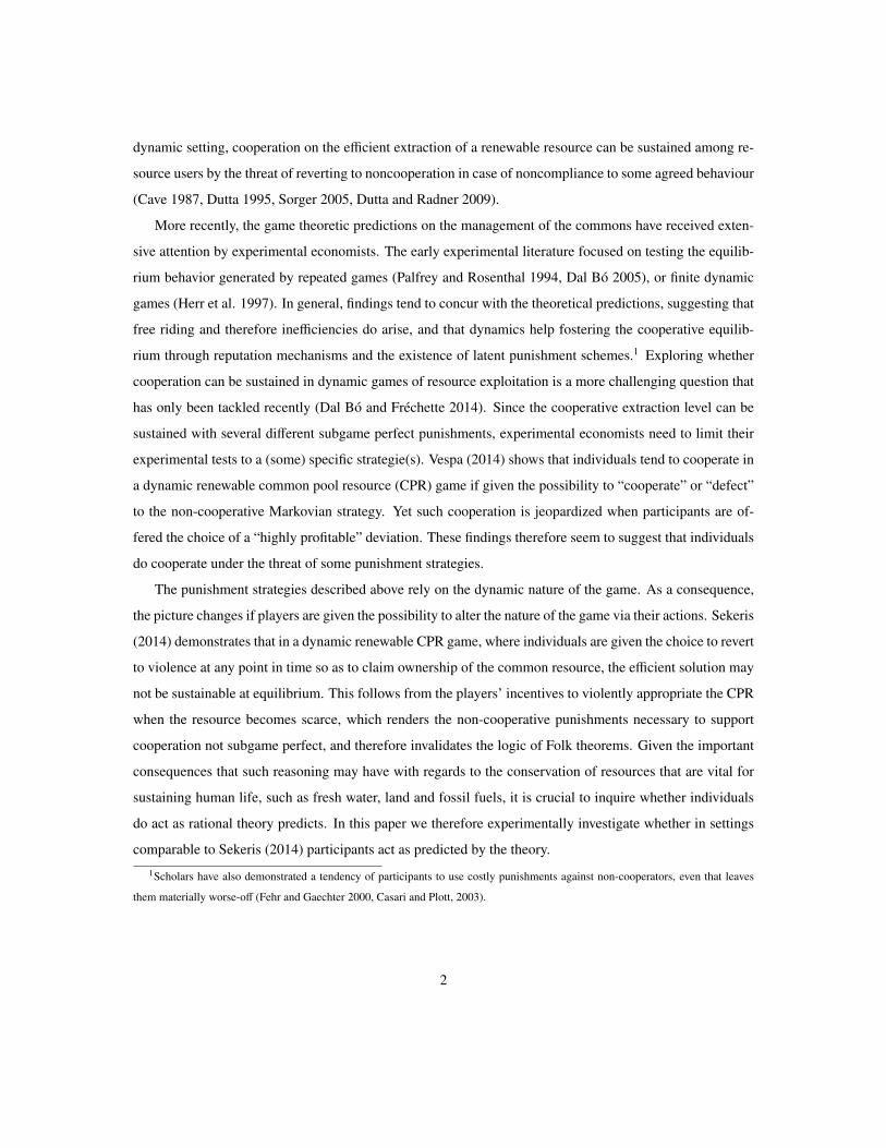
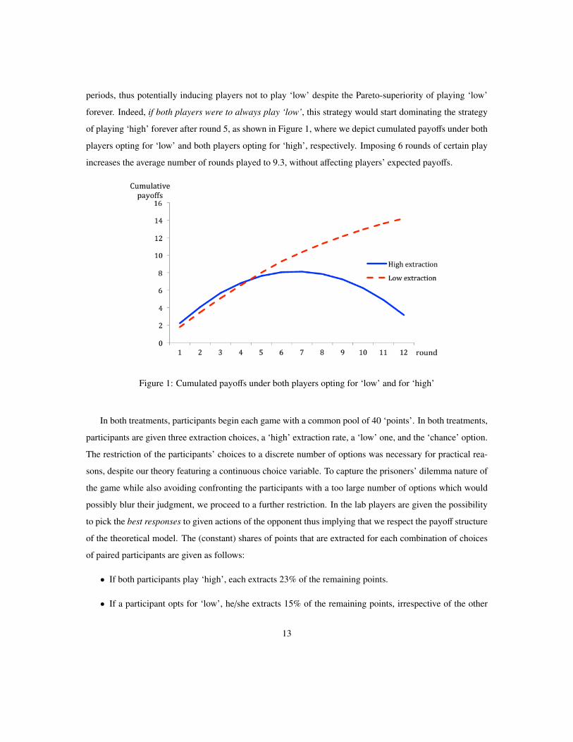
periods, thus potentially inducing players not to play ‘low’ despite the Pareto-superiority of playing ‘low’

forever. Indeed, if both players were to always play ‘low’, this strategy would start dominating the strategy

of playing ‘high’ forever after round 5, as shown in Figure 1, where we depict cumulated payoffs under both

players opting for ‘low’ and both players opting for ‘high’, respectively. Imposing 6 rounds of certain play

increases the average number of rounds played to 9.3, without affecting players’ expected payoffs.

Figure 1: Cumulated payoffs under both players opting for ‘low’ and for ‘high’

In both treatments, participants begin each game with a common pool of 40 ‘points’. In both treatments,

participants are given three extraction choices, a ‘high’ extraction rate, a ‘low’ one, and the ‘chance’ option.

The restriction of the participants’ choices to a discrete number of options was necessary for practical rea-

sons, despite our theory featuring a continuous choice variable. To capture the prisoners’ dilemma nature of

the game while also avoiding confronting the participants with a too large number of options which would

possibly blur their judgment, we proceed to a further restriction. In the lab players are given the possibility

to pick the best responses to given actions of the opponent thus implying that we respect the payoff structure

of the theoretical model. The (constant) shares of points that are extracted for each combination of choices

of paired participants are given as follows:

• If both participants play ‘high’, each extracts 23% of the remaining points.

• If a participant opts for ‘low’, he/she extracts 15% of the remaining points, irrespective of the other

13

participant’s extraction.

• If a participant plays ‘high’ and his/her match plays ‘low’, he/she extracts 25.5% of the remaining

points.

• If either participant plays ‘chance’, he/she retains the control of φ(rt)rt resources, and extracts 30% of

the resources at this round and at the following ones.

If chance is selected, therefore, the CPR is subjected to a loss described by (1−φ(rt))rt with the resilience

function given by (21) in the ‘chance’ treatment, or by (1 − φ)rt = 0.6rt in the ‘costly chance’ treatment.

In both treatments the remaining stock of points is shared equally among both players, who are from then

on imposed the (optimal) ‘low’ level of extraction for the current and all subsequent rounds. Consistent

with the theoretical findings, we expect that, when confronted with the chance treatment, participants should

substitute ‘low’ by ‘high’ in a game’s early rounds, while chance should be selected after the stock of points

drops below 29.15 (i.e. when inequality (20) is satisfied).

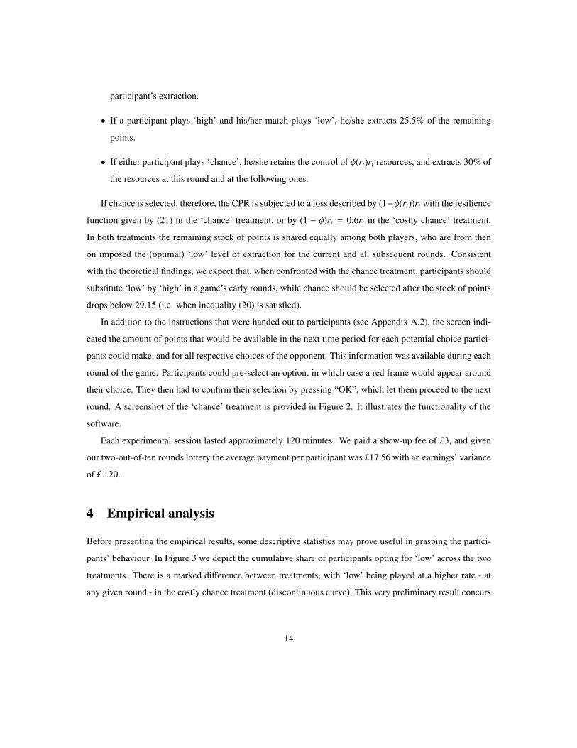
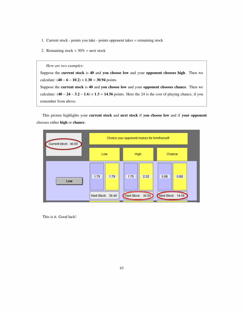
In addition to the instructions that were handed out to participants (see Appendix A.2), the screen indi-

cated the amount of points that would be available in the next time period for each potential choice partici-

pants could make, and for all respective choices of the opponent. This information was available during each

round of the game. Participants could pre-select an option, in which case a red frame would appear around

their choice. They then had to confirm their selection by pressing “OK”, which let them proceed to the next

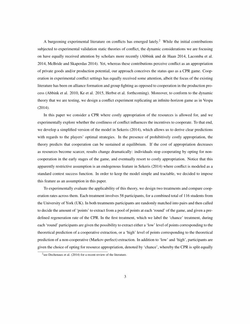
round. A screenshot of the ‘chance’ treatment is provided in Figure 2. It illustrates the functionality of the

software.

Each experimental session lasted approximately 120 minutes. We paid a show-up fee of £3, and given

our two-out-of-ten rounds lottery the average payment per participant was £17.56 with an earnings’ variance

of £1.20.

4 Empirical analysis

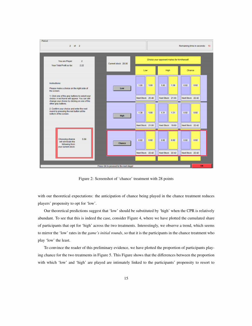
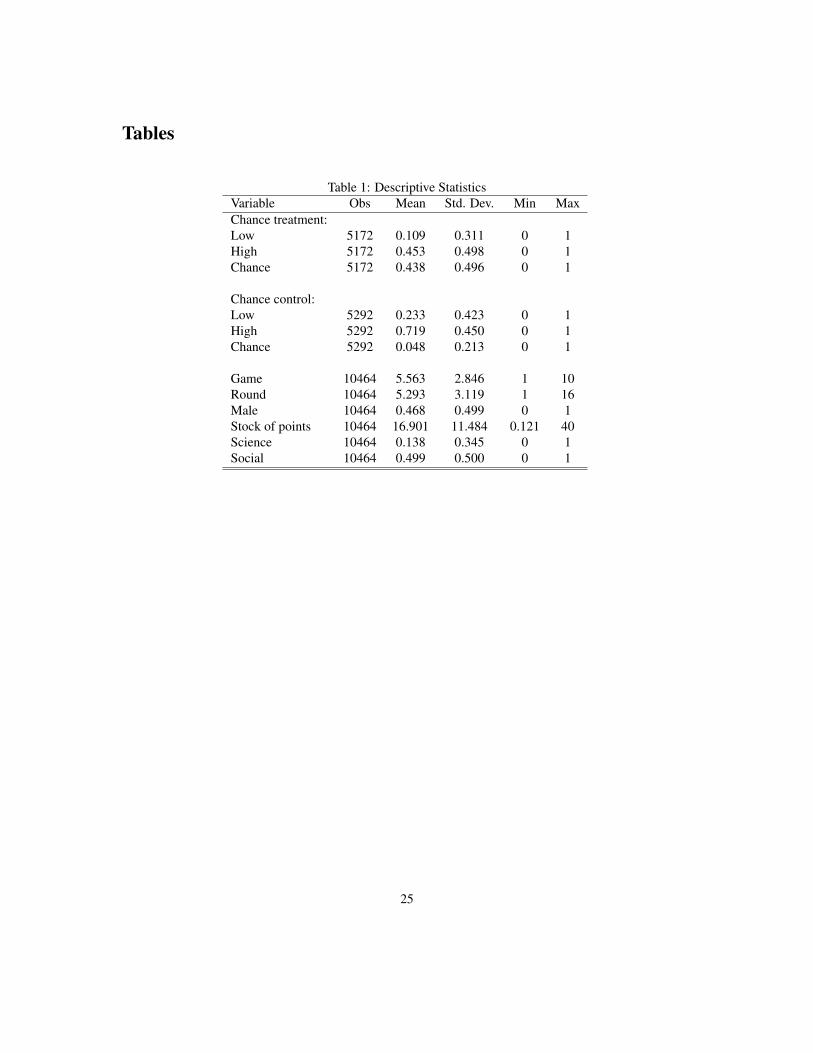
Before presenting the empirical results, some descriptive statistics may prove useful in grasping the partici-

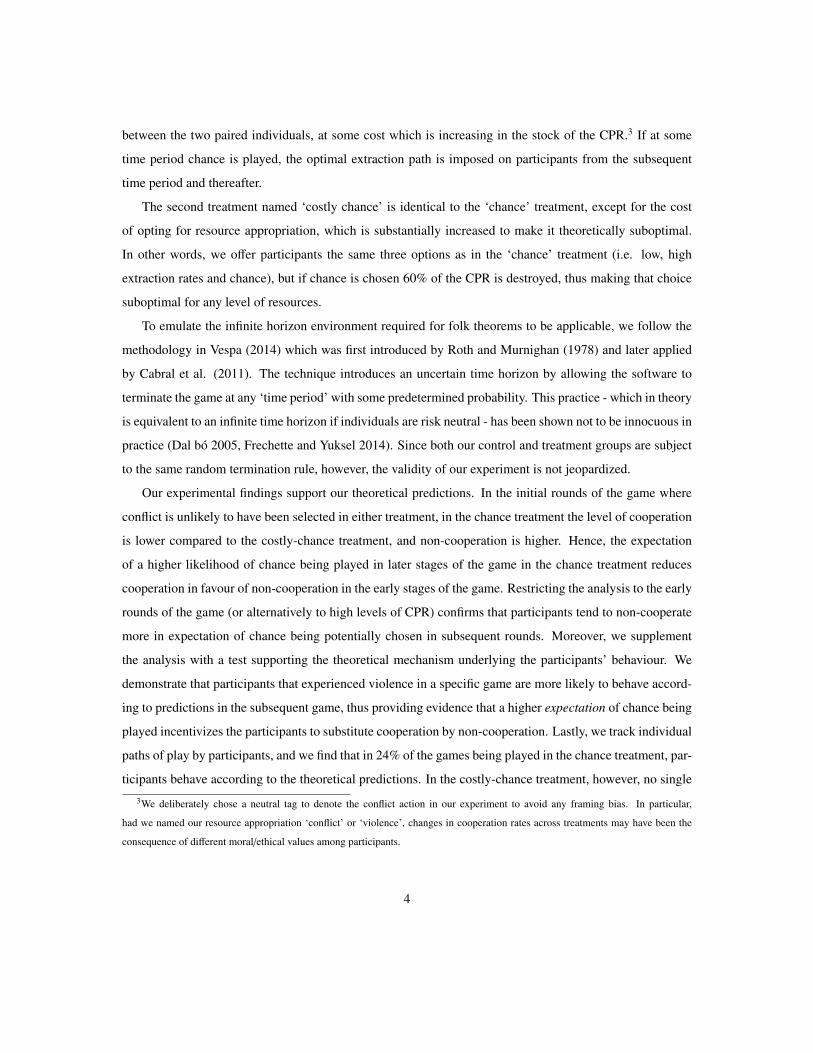
pants’ behaviour. In Figure 3 we depict the cumulative share of participants opting for ‘low’ across the two

treatments. There is a marked difference between treatments, with ‘low’ being played at a higher rate - at

any given round - in the costly chance treatment (discontinuous curve). This very preliminary result concurs

14

Figure 2: Screenshot of ‘chance’ treatment with 28 points

with our theoretical expectations: the anticipation of chance being played in the chance treatment reduces

players’ propensity to opt for ‘low’.

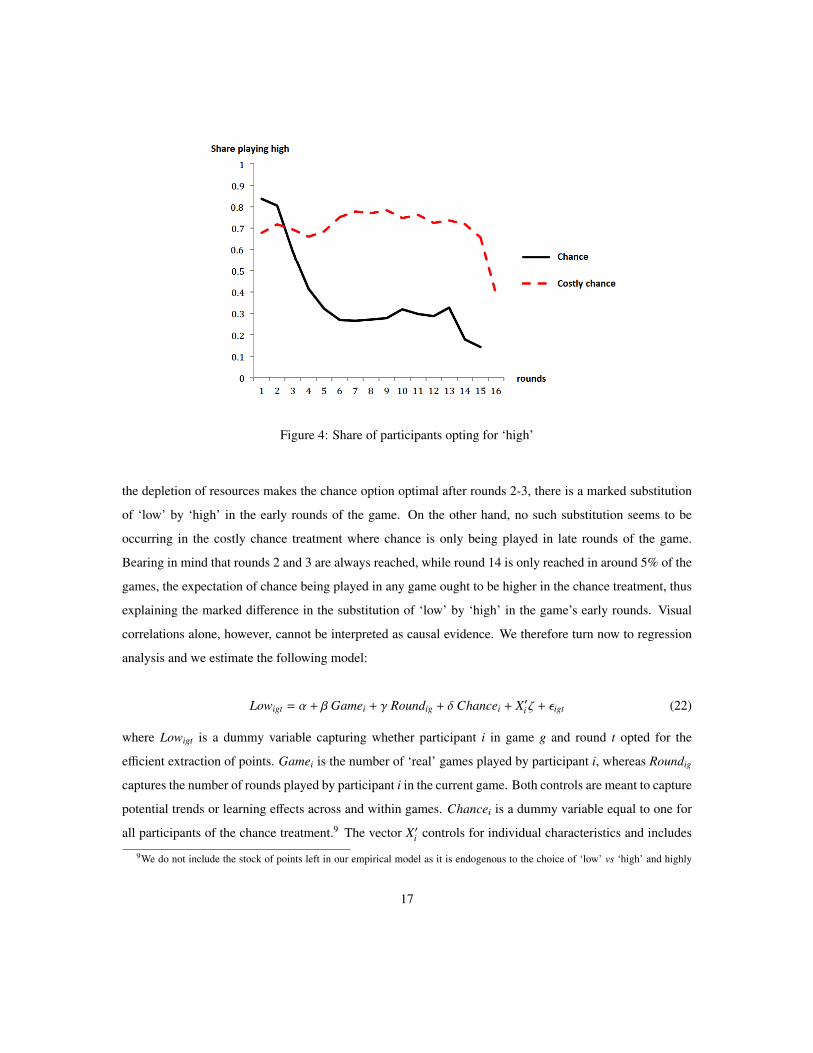
Our theoretical predictions suggest that ‘low’ should be substituted by ‘high’ when the CPR is relatively

abundant. To see that this is indeed the case, consider Figure 4, where we have plotted the cumulated share

of participants that opt for ‘high’ across the two treatments. Interestingly, we observe a trend, which seems

to mirror the ‘low’ rates in the game’s initial rounds, so that it is the participants in the chance treatment who

play ‘low’ the least.

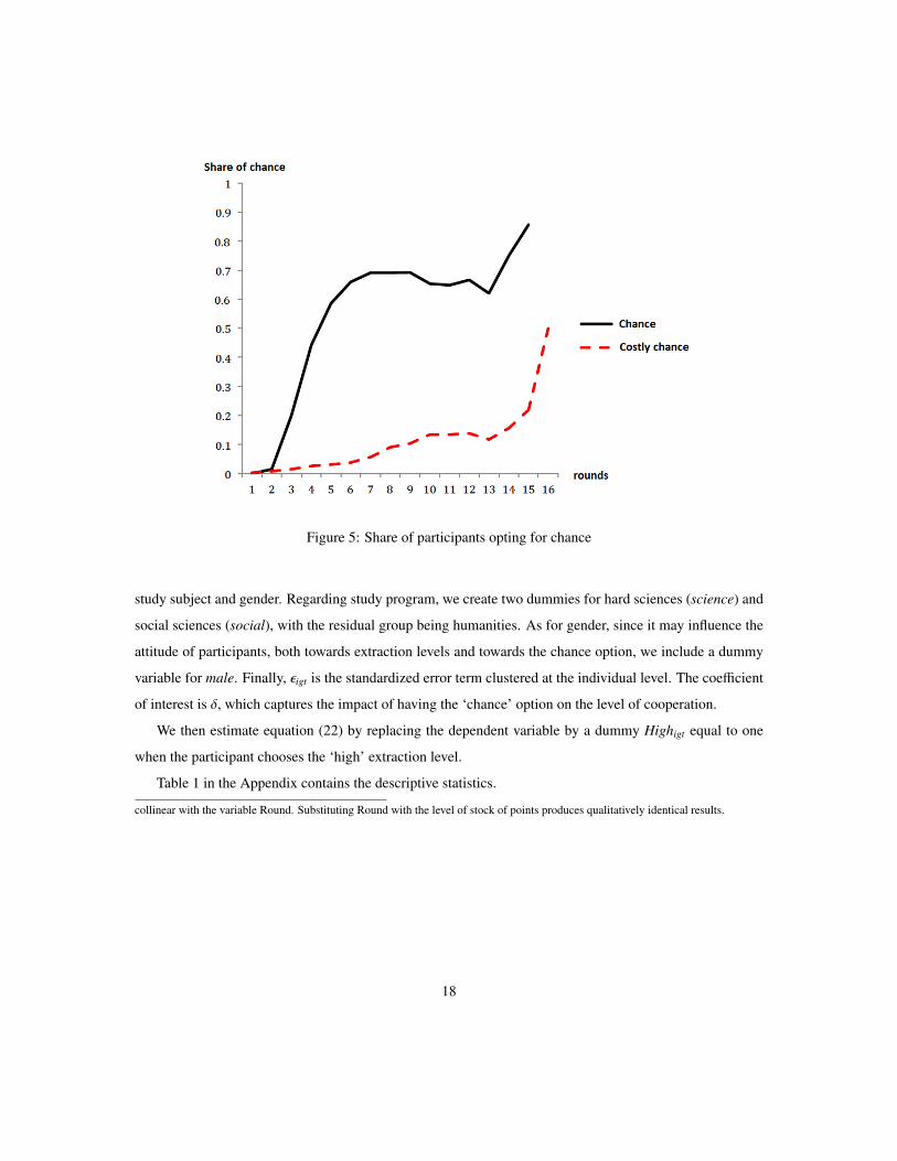
To convince the reader of this preliminary evidence, we have plotted the proportion of participants play-

ing chance for the two treatments in Figure 5. This Figure shows that the differences between the proportion

with which ‘low’ and ‘high’ are played are intimately linked to the participants’ propensity to resort to

15

chance during later rounds of the game. There is a marked difference in the proportion with which chance

is being played in the chance (continuous curve) and the costly-control (dotted curve) treatments. In the

former treatment, participants are more willing to play chance during any round of the game, but perhaps

more importantly, there is a striking difference between the chronological evolution depicted in the sepa-

rate curves. In the chance treatment we observe a sharp increase in round 3, which corresponds to the round

where the level of points is - on average - in the range where chance becomes optimal in theory. Since chance

is never optimal in the chance-control treatment, we should expect no similar pattern in the latter treatment,

which seems to be confirmed by Figure 5. Under both treatments we do, however, observe an increase in the

proportion of participants that play chance in later rounds, and more specifically around round 14. Bearing

in mind the imposed random termination rule, the likelihood that any game reaches round 14 equals 0.057,

thus making it a very unlikely event. In trying to understand this behaviour, several reasons can be invoked.

One could be that participants resort to some sort of protection mechanism by attempting to put an end to the

depletion of the CPR. Other psychological mechanisms could be invoked to explain these observations, but

irrespective of the cause of this behaviour, the only explanation for the differences in the higher propensity

to play ‘high’ in the game’s early rounds must be the differential expectations of such behaviour in the future

(i.e. higher such expectations in the chance treatment).

Figure 3: Share of participants opting for ‘low’

The patterns presented in Figures 3-5 are consistent with our mechanism: in the chance treatment where

16

Figure 4: Share of participants opting for ‘high’

the depletion of resources makes the chance option optimal after rounds 2-3, there is a marked substitution

of ‘low’ by ‘high’ in the early rounds of the game. On the other hand, no such substitution seems to be

occurring in the costly chance treatment where chance is only being played in late rounds of the game.

Bearing in mind that rounds 2 and 3 are always reached, while round 14 is only reached in around 5% of the

games, the expectation of chance being played in any game ought to be higher in the chance treatment, thus

explaining the marked difference in the substitution of ‘low’ by ‘high’ in the game’s early rounds. Visual

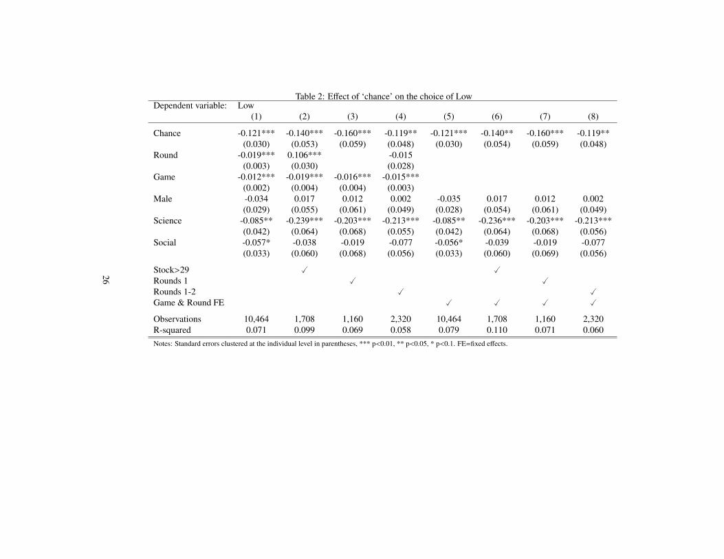
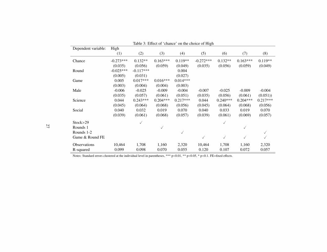
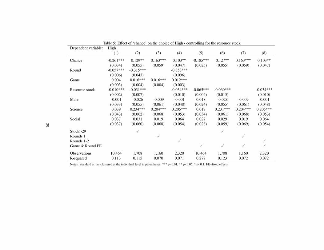
correlations alone, however, cannot be interpreted as causal evidence. We therefore turn now to regression

analysis and we estimate the following model:

Lowigt = α + β Gamei + γ Roundig + δ Chancei + X′i ζ + εigt (22)

where Lowigt is a dummy variable capturing whether participant i in game g and round t opted for the

efficient extraction of points. Gamei is the number of ‘real’ games played by participant i, whereas Roundig

captures the number of rounds played by participant i in the current game. Both controls are meant to capture

potential trends or learning effects across and within games. Chancei is a dummy variable equal to one for

all participants of the chance treatment.9 The vector X′i controls for individual characteristics and includes

9We do not include the stock of points left in our empirical model as it is endogenous to the choice of ‘low’ vs ‘high’ and highly

17

Figure 5: Share of participants opting for chance

study subject and gender. Regarding study program, we create two dummies for hard sciences (science) and

social sciences (social), with the residual group being humanities. As for gender, since it may influence the

attitude of participants, both towards extraction levels and towards the chance option, we include a dummy

variable for male. Finally, εigt is the standardized error term clustered at the individual level. The coefficient

of interest is δ, which captures the impact of having the ‘chance’ option on the level of cooperation.

We then estimate equation (22) by replacing the dependent variable by a dummy Highigt equal to one

when the participant chooses the ‘high’ extraction level.

Table 1 in the Appendix contains the descriptive statistics.

collinear with the variable Round. Substituting Round with the level of stock of points produces qualitatively identical results.

18

4.1 Baseline results

In Table 2 we report the results of estimating model (22).10 In other words, we are evaluating the effect of

having a conflict technology which makes conflict a profitable choice on the propensity to play ‘low’. The

first column of Table 2 reports the results of the benchmark specification. Compared to the costly-chance

control, participants in the chance treatment tend to play ‘low’ by 12.1 percentage points less on average,

thus lending support to our theoretical findings. Given that the average propensity of ‘low’ in the costly-

chance treatment equals 71.9%, this implies that the introduction of the chance option reduces the likelihood

of ‘low’ being played by 16.8%. Consistently with previous findings, the Game coefficient, which captures

the learning effect across games, implies that the propensity of ‘low’ decreases on average by 1.2 percentage

points from one game to another (Dal Bo and Frechette 2011). Moreover, ‘low’ is decreasing on average

by 1.9 percentage point from one round to another within a game. As will become clear later, the latter

result is mainly driven by participants’ increasingly frequent choice of chance, on the one hand, and by the

participants’ increasingly frequent reversion to ‘high’ when the stock of points start to run very low. Lastly,

the gender and studies coefficients take signs compatible with earlier findings: male participants tend to

cooperate less (Eckel and Grossman 1998), and the same holds true for non-humanities students (Frank et

al. 1993).

The negative effect on ‘low’ of allowing participants to use the ‘chance’ option does not necessarily map

onto an increase of ‘high’ to the extent that the effect may be driven by an increase in the use of the third

option, chance, which is sub-optimal in the costly-chance treatment. Proposition 2 stipulates that for high

levels of the stock of points (i.e. r > 29.15 given our parametrization) the optimal decision is to choose

‘high’, with the chance option being used only when the stock of points is sufficiently depleted (r ≤ 29.15).

To verify therefore that we indeed observe a substitution of ‘low’ by ‘high’ in the game’s early rounds, we

restrict our estimation in multiple ways. In column 2 of Table 2, we restrict the sample to r > 29 to see

whether for high stock of points - where chance is unlikely to have been chosen in either treatment - ‘low’

does decrease. Compared to the benchmark estimation (Column 1), the coefficient is larger and significant at

the 1% level, thus implying that ‘low’ decreases as compared to the costly chance treatment, when resorting

to chance is theoretically sub-optimal.

As alternative tests, we restrict the estimation in Columns 3 and 4 to the game’s early rounds. As the

choice of ‘low’ after round 1 is endogenous to the choices of round 1, decisions in subsequent rounds may

10All model specifications are estimated by OLS. Replicating our estimates by a probit estimation does not affect our results qualita-

tively.

19

be influenced by strategic reactions to the opponent’s earlier choices in the same game. Accordingly, in

Column 3 we restrict the analysis to round 1 alone. The coefficient of interest is larger than in the previous

estimations, and significant at the 1% level. In Column 4 we repeat the exercise by restricting the analysis

to the game’s first 2 rounds. Given that all games begin with a stock of 40 points, the stock of points

would equal 28 in round 2, even if both players played ‘high’ in the game’s first rounds, making participants

roughly indifferent between playing ‘chance’ and not in the chance treatment. Cooperation is significantly

lower under the chance treatment by 11.9 percentage points, further confirming our expectations.

Specification 22 considers a linear effect of Round and Game on the dependent variable. To allow for

non-linear effects, we reproduce in Columns 5 − 8 the specifications of Columns 1 − 4 by introducing round

and game fixed effects instead of linear trends. The results remain quantitatively almost unchanged.

In Table 3 we present the results of the same specifications as in Table 2 by replacing the dependent

variable by ‘high’. The benchmark regression yields a negative coefficient, which is significant at the 1%

level: adding the ‘chance’ option reduces ‘high’ on average by 27.3 percentage points compared to the costly

chance treatment. As mentioned earlier, one may be tempted to conclude that in the ‘chance’ option when

playing chance becomes optimal, we observe a reduction of both ‘low’ and ‘high’ in favour of ‘chance’, thus

possibly contradicting Proposition 2. Such an interpretation would be mistaken, however, since the bench-

mark model captures the average effects of the introduction of chance in a standard CPR exploitation game,

while Proposition 2 clearly identifies two distinct optimal choices depending on the stock of points: where

points are abundant ‘high’ should increase, whereas where points are scarce chance is the optimal choice.

We therefore proceed in columns 2-4 with the same sample restrictions as in Table 2. If Proposition 2 is to

be verified, we should expect ‘high’ to increase only when the stock of points is abundant, or alternatively

in the early rounds of the game. Our results confirm this prediction: according to the results reported in

column 4, ‘high’ increases by 16.3 percentage points in the game’s first round compared to the costly chance

treatment. Hence, the availability of “profitable” conflict technology induces participants to substitute ‘low’

with ‘high’ when the stock of points is sufficiently large.

One potential concern could be that since playing chance implies that participants stop making choices

in subsequent rounds of the same game, the decision to play chance could be driven by non-pecuniary

motivations such as putting an early end to the game (playing chance too early) or deferring chance to future

rounds because of the utility derived by playing the game (playing chance too late). Since our theoretical

mechanism identifies a critical resource threshold triggering conflict (i.e. chance), we reproduce Tables 2

and 3 by adding as a control variable the level of resources. The results are contained in Tables 4 and 5. Our

20

results are strongly robust to this additional test.

As explained earlier, the substitution of ‘low’ by ‘high’ in the chance treatment is explained by the sharp

increase of ‘chance’ being played in rounds 3− 6. Indeed, as can be seen in Figure 5 virtually no participant

opts for ‘chance’ in the first 2 rounds of the game. Secondly, we observe a surge of ‘chance’ being chosen

in rounds 3 to 6, rising from it being played by 1.5% to 66% of the pairs. This coincides roughly with our

expectation that chance becomes optimal when the stock of points drops below 29, since the average stock

of points in rounds 2 and 3 is equal to 29 and 21.1 points, respectively. Bearing in mind the relatively low

proportion of participants opting for ‘chance’ in the costly chance treatment, as well as the low probability

of the game lasting long enough (i.e. after round 13) for there to be a real risk of ‘chance’ being played,

this graph supports our story. Combined with the results of Tables 2 and 3, we can confidently state that

the introduction of a profitable (for low levels of resources) appropriation option in an experimental game

of renewable CPR exploitation induces participants to become more non-cooperative in the presence of

abundant resource stocks, thus precipitating their depletion, and eventually opting for the partition of the

resource.

4.2 Exploring the mechanism

4.2.1 The expectation of chance

To further convince the reader that it is indeed the expectation of chance being played that triggers ‘high’

in the game’s early rounds, we explore whether higher expectations of ‘chance’ being played reinforces

the behaviour patterns compatible with our theory. If the substitution of ‘low’ by ‘high’ observed in the

early rounds of the chance treatment rests in the expectation of ‘chance’ being played, we should expect

participants who choose ‘chance’ (‘attackers’), and those matched with them (‘victims’) in the previous

game, to increase their expectation for chance to be played. While the attackers’ behaviour may be driven

by unobserved characteristics equally explaining their previous decision to opt for ‘chance’, the potential

alteration of the victims’ behaviour would reveal some information updating on behalf of the participants,

who would now be expecting ‘chance’ to be played with a higher probability. This, in turn, implies that past

attackers, and even more so past victims, should more markedly reduce ‘low’ and increase ‘high’ in the early

rounds of a game.

To implement this test we create two additional variables: a dummy capturing whether a participant has

played chance in the previous game (lagged attacker) and another dummy capturing whether a participant

21

was matched with an attacker in the previous game (lagged victim). We then re-estimate our models, includ-

ing these two additional controls. The results of this test are reported in Tables 6 and 7. The first 3 columns

of both tables replicate columns 2 − 4 of Tables 2 and 3, respectively.

The results in column 1 of Table 6 suggest that, when the stock of points is higher than 29 points, previous

game attackers play ‘low’ by 8.1 percentage points less than the average participant in the chance treatment.

The equivalent figure for victims in the previous game equals 7.7 percentage points. The equivalent values

for ‘high’ as contained in Column 1 of Table 7 equal 5.3 and 7.8 percentage points, respectively. This

suggests that lagged victims fully substitute their reduced propensity to play ‘low’ by ‘high’ when resources

are abundant. On the other hand, lagged attackers seem to substitute ‘low’ by a mixture of ‘high’ and

‘chance’. This considerable difference between participants who did not experience chance in the previous

game, and those who did, further supports that the expectation of chance is the mechanism driving the

substitution of ‘low’ by ‘high’. Results in columns 2&3 of both tables follow a similar pattern, thus further

strengthening our interpretation. In Columns 4 − 6 of both tables we substitute round and game trends by

round and game fixed effects. The results remain unaffected.

Finally we replicate the same exercise but restricting the analysis on participants in the chance treatment.

We therefore test whether participants that experience ‘chance’ in the previous game, as an attacker or as

a victim, are more likely to play ‘high’ and less likely to play ‘low’ in the early periods of the game. The

results, reported in Tables 8 and 9 broadly confirm our previous results. We can thus confidently deduce that

participants who have experienced ‘chance’ in the previous game are more likely to expect ‘chance’ to be

chosen in the current game, therefore substituting ‘low’ by ‘high’ in the game’s early rounds.

4.2.2 Tracking individual paths of play

To further convince the reader that the mechanism identified in our theoretical framework is actually the one

driving our experimental results, we provide some additional supportive evidence based on the individual

play-paths of our participants. The theory predicts that in the chance treatment participants should play h for

two rounds, before opting for c. In the costly chance treatment, on the other hand, no similar pattern should

be observed since conflict is theoretically suboptimal. Interestingly, out of 580 participant-game play paths

(i.e. 58 participants each playing separate 10 games), 77 perfectly match the theoretical expectations. In

other words, in 13.3% of the participant-games, the participants opted for the sequence {h, h, c}. In the costly

chance treatment on the other hand this was never the case.

Given that computing the precise optimal round where conflict should be played in the chance treatment

22

may involve a significant level of sophistication on behalf of the participants, we equally explore the number

of participant-game play paths where chance was chosen in rounds 4 and 5, respectively, following a contin-

uous sequence of h choices. The respective number of participant-games following such sequences are 38

for the sequence {h, h, h, c}, and 24 for the sequence {h, h, h, h, c}. In total, this implies that if we adopt a less

stringent reading of our theory, about 24% of the participant-game play paths matching the sequence of ac-

tions compatible with our theory. This figure is particularly salient given that in the costly chance treatment

not a single instance of a participant-game matches either of the above sequences of play. These findings

constitute strong evidence that our results do not merely reflect behaviour compatible with the theoretical

results on average, but instead that the mechanism is verified for a large share of participants at the individual

level.

5 Conclusion

Folk theorems permit cooperation to arise in equilibrium in dynamic common pool renewable resource

games, both theoretically and experimentally. Allowing the players to revert to violence to split the re-

source (and to thereafter manage efficiently what has become a private resource) disrupts the logic of Folk

theorems. In our theoretical section we propose a simple version of the CPR management model of Sek-

eris (2014), where players can opt for potentially costly conflict to share resources. In the presence of a

highly destructive conflict technology, violence is never optimal, and thus cooperation is sustainable. With

conflict technologies making conflict profitable under some circumstances, infinite horizon dynamic games

may endogenously become finite horizon strategic games up to the moment when conflict emerges, after

which the problem stops being strategic and instead becomes decision-theoretic. This deprives players of

the required punishment strategy for sustaining cooperation, thereby leading to the collapse of cooperation.

In this paper we inquire experimentally whether participants respond to such incentives that should lead to

(i) less cooperation in the presence of high stocks of resources, and to (ii) conflict after the resource stock

is sufficiently depleted. We find a strong and highly significant effect of conflict on the choices of coopera-

tion and non-cooperation. In the game’s first round, participants reduce their cooperation by 16 percentage

points and increase non-cooperation by 16.3 percentage points. Given that the average rates of cooperation

and non-cooperation in the game’s first round are around 24.1% and and 75.7%, respectively, this equates,

to a 66% decrease of cooperation, and to a 21% increase of non-cooperation.

To provide further evidence of the theoretical mechanism proposed in this paper, we equally proceeded

23

to two additional verification tests. We explored whether having experienced chance in the previous game

being played as an attacker or a victim increases the participants’ inclination to play according to the theo-

retical results. The findings unambiguously point towards an increased substitution of cooperation by non-

cooperation among both lagged attackers and lagged victims. This confirms that the experience of conflict

in a previous game increases the expectation among these participants of conflict occurring in the ongoing

game, in turn leading to less cooperative behaviour. The second verification exercise consisted in tracking

the sequence of choices made by participants in games. We find that in the chance treatment about 24% of

the participant-game play paths match the sequence of actions compatible with our theory, compared with

0% in the costly-chance treatment. We interpret these figures as strong evidence that our experimental find-

ings are driven by the participants’ individual behaviour rather than by average effects, thus allowing us to

confidently conclude that participants behave as predicted by our theory.

This contribution constitutes the first evidence that the fear of - possibly distant - conflicts over shared

resources can hamper cooperation in the short run, and can thereby accelerate the depletion of the resources.

Our findings may help comprehend the failure to reach agreements over such matters as the conservation of

the environment. This in turn would imply that one crucial dimension for promoting cooperation would be

the strengthening of institutions and international bodies able to contain such violence.

Acknowledgments

This project has benefited from the financial support of the Universities of Portsmouth and York.

24

Tables

Table 1: Descriptive StatisticsVariable Obs Mean Std. Dev. Min MaxChance treatment:Low 5172 0.109 0.311 0 1High 5172 0.453 0.498 0 1Chance 5172 0.438 0.496 0 1

Chance control:Low 5292 0.233 0.423 0 1High 5292 0.719 0.450 0 1Chance 5292 0.048 0.213 0 1

Game 10464 5.563 2.846 1 10Round 10464 5.293 3.119 1 16Male 10464 0.468 0.499 0 1Stock of points 10464 16.901 11.484 0.121 40Science 10464 0.138 0.345 0 1Social 10464 0.499 0.500 0 1

25

Table 2: Effect of ‘chance’ on the choice of LowDependent variable: Low

(1) (2) (3) (4) (5) (6) (7) (8)

Chance -0.121*** -0.140*** -0.160*** -0.119** -0.121*** -0.140** -0.160*** -0.119**(0.030) (0.053) (0.059) (0.048) (0.030) (0.054) (0.059) (0.048)

Round -0.019*** 0.106*** -0.015(0.003) (0.030) (0.028)

Game -0.012*** -0.019*** -0.016*** -0.015***(0.002) (0.004) (0.004) (0.003)

Male -0.034 0.017 0.012 0.002 -0.035 0.017 0.012 0.002(0.029) (0.055) (0.061) (0.049) (0.028) (0.054) (0.061) (0.049)

Science -0.085** -0.239*** -0.203*** -0.213*** -0.085** -0.236*** -0.203*** -0.213***(0.042) (0.064) (0.068) (0.055) (0.042) (0.064) (0.068) (0.056)

Social -0.057* -0.038 -0.019 -0.077 -0.056* -0.039 -0.019 -0.077(0.033) (0.060) (0.068) (0.056) (0.033) (0.060) (0.069) (0.056)

Stock>29 � �Rounds 1 � �Rounds 1-2 � �Game & Round FE � � � �

Observations 10,464 1,708 1,160 2,320 10,464 1,708 1,160 2,320R-squared 0.071 0.099 0.069 0.058 0.079 0.110 0.071 0.060Notes: Standard errors clustered at the individual level in parentheses, *** p<0.01, ** p<0.05, * p<0.1. FE=fixed effects.

26

Table 3: Effect of ‘chance’ on the choice of HighDependent variable: High

(1) (2) (3) (4) (5) (6) (7) (8)

Chance -0.273*** 0.132** 0.163*** 0.119** -0.272*** 0.132** 0.163*** 0.119**(0.035) (0.056) (0.059) (0.049) (0.035) (0.056) (0.059) (0.049)

Round -0.025*** -0.117*** 0.004(0.005) (0.031) (0.027)

Game 0.005 0.017*** 0.016*** 0.014***(0.003) (0.004) (0.004) (0.003)

Male -0.006 -0.025 -0.009 -0.004 -0.007 -0.025 -0.009 -0.004(0.035) (0.057) (0.061) (0.051) (0.035) (0.056) (0.061) (0.051))

Science 0.044 0.243*** 0.204*** 0.217*** 0.044 0.240*** 0.204*** 0.217***(0.045) (0.064) (0.068) (0.056) (0.045) (0.064) (0.068) (0.056)

Social 0.040 0.032 0.019 0.070 0.040 0.033 0.019 0.070(0.039) (0.061) (0.068) (0.057) (0.039) (0.061) (0.069) (0.057)



27

Table 4: Effect of ‘chance’ on the choice of Low - controlling for the resource stockDependent variable: Low

(1) (2) (3) (4) (5) (6) (7) (8)

Chance -0.129*** -0.136** -0.160*** -0.100** -0.150*** -0.135** -0.160*** -0.100**(0.029) (0.053) (0.059) (0.044) (0.029) (0.052) (0.059) (0.044)

Round 0.001 0.324*** 0.426***(0.005) (0.044) (0.069)

Game -0.011*** -0.017*** -0.016*** -0.013***(0.002) (0.004) (0.004) (0.003)

Resource stock 0.006*** 0.035*** 0.042*** 0.021*** 0.063*** 0.041***(0.002) (0.007) (0.007) (0.003) (0.015) (0.007)

Male -0.037 0.018 0.012 -0.002 -0.043* 0.020 0.012 -0.002(0.027) (0.053) (0.061) (0.046) (0.025) (0.053) (0.061) (0.046)

Science -0.082** -0.230*** -0.203*** -0.198*** -0.077* -0.226*** -0.203*** -0.198***(0.041) (0.062) (0.068) (0.052) (0.039) (0.061) (0.068) (0.052)

Social -0.055* -0.037 -0.019 -0.070 -0.052* -0.034 -0.019 -0.070(0.032) (0.058) (0.068) (0.052) (0.030) (0.058) (0.069) (0.052)



28

Table 5: Effect of ‘chance’ on the choice of High - controlling for the resource stockDependent variable: High

(1) (2) (3) (4) (5) (6) (7) (8)

Chance -0.261*** 0.129** 0.163*** 0.103** -0.185*** 0.127** 0.163*** 0.103**(0.034) (0.055) (0.059) (0.047) (0.025) (0.055) (0.059) (0.047)

Round -0.057*** -0.315*** -0.353***(0.006) (0.043) (0.096)

Game 0.004 0.016*** 0.016*** 0.012***(0.003) (0.004) (0.004) (0.003)

Resource stock -0.010*** -0.031*** -0.034*** -0.065*** -0.060*** -0.034***(0.002) (0.007) (0.010) (0.004) (0.015) (0.010)

Male -0.001 -0.026 -0.009 -0.001 0.018 -0.028 -0.009 -0.001(0.033) (0.055) (0.061) (0.048) (0.024) (0.055) (0.061) (0.048)

Science 0.039 0.234*** 0.204*** 0.205*** 0.017 0.231*** 0.204*** 0.205***(0.043) (0.062) (0.068) (0.053) (0.034) (0.061) (0.068) (0.053)

Social 0.037 0.031 0.019 0.064 0.027 0.029 0.019 0.064(0.037) (0.060) (0.068) (0.054) (0.028) (0.059) (0.069) (0.054)



29

Table 6: The impact of experiencing chance in the past on LowDependent variable: Low

(1) (2) (3) (4) (5) (6)

Chance -0.100* -0.114* -0.082 -0.097* -0.112* -0.080(0.056) (0.062) (0.052) (0.057) (0.063) (0.052)

Lagged attacker -0.081* -0.080 -0.059 -0.085* -0.084 -0.062(0.044) (0.052) (0.042) (0.045) (0.052) (0.043)

Lagged victim -0.077** -0.067** -0.070*** -0.078** -0.070** -0.072***(0.032) (0.033) (0.026) (0.033) (0.033) (0.026)

Round 0.085** -0.013(0.033) (0.029)

Game -0.014*** -0.013*** -0.012***(0.004) (0.004) (0.003)

Male 0.020 0.014 0.003 0.020 0.014 0.003(0.053) (0.060) (0.047) (0.053) (0.060) (0.047)

Science -0.229*** -0.193*** -0.204*** -0.226*** -0.193*** -0.203***(0.059) (0.065) (0.052) (0.059) (0.066) (0.052)

Social -0.040 -0.023 -0.079 -0.040 -0.023 -0.079(0.060) (0.067) (0.054) (0.059) (0.068) (0.054)

Stock>29 � �Rounds 1 � �Rounds 1-2 � �Game & Round FE � � �

Observations 1,508 1,044 2,088 1,508 1,044 2,088R-squared 0.089 0.069 0.058 0.099 0.072 0.061Notes: Standard errors clustered at the individual level in parentheses, *** p<0.01, ** p<0.05, * p<0.1.

A Appendix

A.1 ProofsA.1.1 Derivation of the optimal extraction rate under conflict

We denote by Vci (ri,t) the value function of this problem given the resource stock ri,t, meaning that the indirect

aggregate utility can be expressed as a Bellman equation:

Vci (ri,t) = arg max

ei,t

[ln

(xi,t

)+ δVc (

ri,t+1)]

(23)

Given the assumed regeneration rule, the above expression can be written as:

30

Table 7: The impact of experiencing chance in the past on HighDependent variable: High

(1) (2) (3) (4) (5) (6)

Chance 0.099* 0.121* 0.089* 0.096* 0.119* 0.087(0.057) (0.063) (0.053) (0.058) (0.063) (0.053)Lagged attacker 0.053 0.073 0.036 0.057 0.076 0.039(0.053) (0.053) (0.049) (0.054) (0.054) (0.049)Lagged victim 0.078** 0.065* 0.070*** 0.080** 0.067** 0.072***(0.032) (0.034) (0.026) (0.033) (0.034) (0.027)Round -0.100*** 0.002(0.033) (0.028)Game 0.013*** 0.013*** 0.012***(0.004) (0.004) (0.003)Male -0.026 -0.010 -0.003 -0.026 -0.010 -0.003(0.054) (0.060) (0.049) (0.054) (0.060) (0.049)Sciance 0.233*** 0.196*** 0.209*** 0.231*** 0.195*** 0.209***(0.059) (0.065) (0.053) (0.059) (0.066) (0.053)Social 0.034 0.022 0.071 0.034 0.022 0.071(0.061) (0.067) (0.056) (0.060) (0.068) (0.056)


Observations 1,508 1,044 2,088 1,508 1,044 2,088R-squared 0.087 0.070 0.055 0.095 0.073 0.057Notes: Standard errors clustered at the individual level in parentheses, *** p<0.01, ** p<0.05, * p<0.1.

31

Table 8: The impact of experiencing chance in the past on Low - chance treatment onlyDependent variable: Low

(1) (2) (3) (4) (5) (6)

Lagged attacker -0.097** -0.071 -0.083* -0.099** -0.072 -0.082*(0.048) (0.060) (0.046) (0.047) (0.060) (0.046)

Lagged victim -0.080** -0.056 -0.077*** -0.079** -0.054 -0.076**(0.034) (0.037) (0.029) (0.034) (0.036) (0.029)

Round 0.072 0.015 0.067 0.015(0.046) (0.038) (0.046) (0.038)

Game -0.015*** -0.012** -0.014***(0.005) (0.006) (0.004)

Male -0.061 -0.058 -0.056 -0.060 -0.058 -0.056(0.068) (0.070) (0.058) (0.068) (0.071) (0.058)

Science -0.101 -0.098 -0.134** -0.102 -0.097 -0.134**(0.074) (0.072) (0.061) (0.074) (0.073) (0.062)

Social 0.023 0.027 -0.042 0.023 0.027 -0.042(0.083) (0.081) (0.071) (0.083) (0.082) (0.071)


Observations 674 522 1,044 674 522 1,044R-squared 0.056 0.038 0.048 0.061 0.045 0.050Notes: Standard errors clustered at the individual level in parentheses, *** p<0.01, ** p<0.05, * p<0.1.

32

Table 9: The impact of experiencing chance in the past on High - chance treatment onlyDependent variable: High

(1) (2) (3) (4) (5) (6)

Lagged attacker 0.068 0.071 0.062 0.070 0.072 0.062(0.059) (0.060) (0.052) (0.059) (0.060) (0.053)

Lagged victim 0.080** 0.056 0.077*** 0.078** 0.054 0.076**(0.033) (0.037) (0.029) (0.034) (0.036) (0.029)

Round -0.126** -0.033 -0.122** -0.033(0.052) (0.034) (0.053) (0.034)

Game 0.014*** 0.012** 0.014***(0.005) (0.006) (0.004)

Male 0.043 0.058 0.048 0.041 0.058 0.048(0.073) (0.070) (0.063) (0.073) (0.071) (0.063)

Science 0.115 0.098 0.144** 0.116 0.097 0.144**(0.076) (0.072) (0.065) (0.076) (0.073) (0.065)

Social -0.030 -0.027 0.033 -0.030 -0.027 0.033(0.083) (0.081) (0.073) (0.083) (0.082) (0.073)


Observations 674 522 1,044 674 522 1,044R-squared 0.059 0.038 0.041 0.064 0.045 0.043Notes: Standard errors clustered at the individual level in parentheses, *** p<0.01, ** p<0.05, * p<0.1.

33

Vci (ri,t) = arg max

ei,t

[ln

(xi,t

)+ δVc

i((1 + γ)

(ri,t − xi,t

))](24)

Differentiating (31) with respect to ei,t, we obtain the following equation:

∂Vci (ri,t)∂ei,t

=1

xci (ri,t)

− δ(1 + γ)Vci′ (

(1 + γ)(rit − xc

i(ri,t

)))= 0 (25)

We next inquire whether ei,t(ri,t) can be a linear in the stock of resources so that ei,t(ri,t) = scri,t. This

assumption implies that the stock of resources in time t+1 equals ri,t+1 = (1+γ)(1− sc)ri,t so that the player’s

indirect utility now reads as:

Vci (ri,t) =

[ln(scri,t) + δ ln

(scri,t(1 + γ)(1 − sc)ri,t

)+ δ2 ln

(scri,t(1 + γ)2(1 − sc)2ri,t

)+ . . .

](26)

Factoring yields:

Vci (ri,t) =

ln(scri,t)1 − δ

+

∞∑t=0

δt ln((1 + γ)t(1 − sc)t

)(27)

Thus implying that:

Vci′

(ri,t) =1

(1 − δ)ri,t(28)

This is turn allows to re-write (25) as:

1scri,t

−δ(1 + γ)

(1 − δ)(1 + γ)(ri,t − scri,t)⇔ sc = 1 − δ (29)

A.1.2 Derivation of the cooperative extraction rate

We denote by Vc(rt) the value function of this problem given the resource stock rt, meaning that the indirect

aggregate utility can be expressed as a Bellman equation:

Vc(rt) = arg maxe1,t ,e2,t

∑i=1,2

ln(xi,t

)+ δVc (rt+1)

(30)

Given the assumed regeneration rule, the above expression can be written as:

Vc(rt) = arg maxe1,t ,e2,t

∑i=1,2

ln(xi,t

)+ δVc (

(1 + γ)(rt − x1,t − x2,t

)) (31)

34

Differentiating (31) with respect to the two decision variables, e1,t and e2,t, we obtain the following

system of equations:

∂Vc(rt)∂e1,t

= 1xc

1(rt)− δ(1 + γ)

∑i=1,2 Vc

i′((1 + γ)

(rt − xc

1 (rt) − xc2 (rt)

))= 0

∂Vc(rt)∂e2,t

= 1xc

2(rt)− δ(1 + γ)

∑i=1,2 Vc

i′((1 + γ)

(rt − xc

1 (rt) − xc2 (rt)

))= 0

(32)

Where these equations hold because the constraint e1,t + e2,t ≤ rt will never be binding, as limrt→0 Vci′

=

+∞.

From (32) we deduce that xc1(rt) = xc

2(rt) = xc(rt). To derive the efficient equilibrium, we inquire whether

xc(rt) may be a linear function of its argument so that xc(rt) = scrt. This assumption implies that the stock

of resources in time period t + 1 can be expressed as rt+1 = (1 + γ) (1 − 2sc) rt. Replacing in Vci , together

with using the regeneration rule gives us:

Vc(rt) = 2[ln (scrt) + δ ln (sc(1 + γ)(1 − 2sc)rt) + δ2 ln

(sc(1 + γ)2(1 − 2sc)2rt

)+ . . .

](33)

Rearranging the terms of (33) gives us:

Vc(rt) =2 ln (scrt)

1 − δ+ 2

∞∑τ=0

δτ ln ((1 + γ)τ(1 − 2sc)τ) (34)

Thus implying that Vc′ (rt) = 2(1−δ)rt

. Substituting in (32) for Vc′ (.) yields:

1scrt−

2δ(1 + γ)(1 − δ)(1 + γ)(1 − 2sc)rt

⇒ sc =1 − δ

2

A.1.3 Derivation of expression (18)

We first need to compute the deviation extraction rate in time period t. This extraction rate is determined by

maximizing player i’s intertemporal payoff, by imposing that in time period t player j chooses his cooperative

extraction rate, while from period t + 1 onwards both players choose their (Markov perfect) non-cooperative

extraction rates. Player i’s optimization problem therefore reads as:

maxx

ln(x) + δVnc((

rt − x −1 − δ

2

)(1 + γ

)Replacing for the appropriate values and optimizing yields the optimal extraction rate xdev given by:

xdev =(1 − δ)(1 + δ)

2(35)

35

Replacing in the regeneration rate implies that:

rt+1 =δ(δ + 1)(1 + γ)

2

Replacing in expression (11) yields:

ln(

(1 − δ)(1 + δ)2

rt

)+

δ

1 − δln

((1 − δ)(1 + γ)δ(1 + δ)

2(2 − δ)rt

)+

δ2

(1 − δ)2 ln(δ(1 + γ)

2 − δ

)<

11 − δ

ln(

1 − δ2

rt

)+

δ

(1 − δ)2 ln(

1 − δ2

)(36)

Simplilfying yields:

(1 − δ) ln(1 + δ) + δ ln(

12 − δ

)< 0

which straightforwardly gives expression (18).

36

A.2 FOR ONLINE PUBLICATION - Instructions to the chance treatment

In this section we present the instruction handed to the chance treatment alone. The chance-control group

received the same instructions, with the difference that the cost of chance was maintained equal to 60%

of the resources throughout, while the no-chance-treatment was presented with the two choices ‘low’ and

‘high’ alone.

Welcome,

You are about to participate in an experiment on decision-making. You will be paid for your participation

in cash, privately, at the end of the session. What you earn depends partly on your decisions, partly on the

decisions of others, and partly on chance.

Please turn off all electronic devices now.

The entire experiment will take place through computer terminals. Please do not talk or in any way try

to communicate with other participants until everybody has been told that the experiment is over and that

you can leave the room.

We will now give you some time to carefully read the following instructions. If you have any questions,

please raise your hand and your question will be answered so everyone can hear.

Overview & Payment

In this experiment you will play the same game 20 times. Each time you play, the computer will

randomly pair you up with someone else in the room (but you don’t know with whom). So, in each game

you are paired with a random person in the room. The first 10 games you play will be for practice. The

remaining 10 games will be for real.

Each game lasts for at least 6 rounds. After the 6th round, you will enter each next round with a proba-

bility of 70% (so with a 30% probability the game ends). So, if you happen to enter round 7, there is a 70%

share that you will enter round 8 and so on and so forth.

When you have played the game 10 times, each game lasting 6 or more rounds, you will be paid. Your

payment has two components, an initial endowment of £5 and a payment of £1.50 per point won. To

establish how many points you have won, we will randomly draw 2 of the last 10 games (the for-real

games) you played and pay you according to the amount of points you won in those games. So, your final

payment will be your initial endowment plus your points payment.

37

Here is an example:

Say, the random draws were games 4 and 6, and you won 5.6 points and 2.4 points in those games

respectively. Then your final payment would be: 3 + (5.6 + 2.4) x 1.50 = £15.

Depending on how you play and for how many rounds the game continues, it is possible that you will

get negative points, though this is unlikely.

Here is another example:

Say, the random draws were games 4 and 6, and you got -2.4 points and 1.2 points in those games

respectively. Then your final payment would be: 3 + (-1.2 + 2.4) x 1.50 = £4.80.

So, to conclude, the choices you make really matter.

Playing a game

At the beginning of each game, you and your opponent both start with a joint stock of 40 points. Each

round, you can choose how much of this stock of points you want to take. Whatever you and your opponent

choose each round will affect how much stock there will be left next round.

The game continues like this. In the second round you choose how much to take of the remaining stock

and that will affect how much stock will be left in round 3, and so on and so forth, until the game ends.

So, there are two things to understand: choice and stock.Your choices are:

• Low

• High

• Chance

Low:

If you choose low and your opponent chooses low too, you each take 15% of the points in stock (e.g. 15%

of 40 points = 6 points).

If you choose low and your opponent chooses high, you take 15% of the points (e.g. 15% of 40 points =

6) and your opponent takes 25.5% of the points (25.5% of 40 points = 10.2).

If you choose low but your opponent chooses chance, then you are in chance mode. What this means is

described below.

38

High:

If you choose high and your opponent chooses low, you take 25.5% of the points (25.5% of 40 points =

10.2) and your opponent takes 15% of the points (15% of 40 points = 6).

If you choose high and your opponent chooses high too, you each take 23% of the points (23% of 40 points

= 9.2 points).

If you choose high but your opponent chooses chance, then you are in chance mode (described below).

Chance:

If either you or your opponent pick chance, then both of you will be in chance mode.

If one of you has played chance, (so that you are both in chance mode) you will each take 15% of the stock

in all of the remaining rounds. As explained more in detail below, the total number of points you will collect

is entirely left to chance under this scenario since you will not be making any more decisions after picking

this option.

Playing chance is costly. Once chance is chosen, a cost will be taken away from your joint stock. The

cost is a one-off loss of points, so it will only be applied once when you enter chance mode, but not in

subsequent rounds of chance mode. Depending on the size of the current stock, this is how much playing

chance would cost:

Stock: 40 39 38 37 36 35 34 33 32 31 30 29 28 27 26 25 24 . . . 0Cost: 24 21.8 19.8 17.8 15.8 14 12.2 10.6 9 7.4 6 4.6 3.4 2.2 1 0 0 . . . 0

There is more to know about your choices:

The points that you take from the current stock each round are not exactly the points that you get to keep.

There is a formula, which describes how many points you get to keep each round.

This will involve some mathematics, i.e. the natural logarithm. If you don’t like maths, don’t worry about

understanding what logarithm means. All you need to know is that the natural logarithm of something is

quite a bit less than that something.

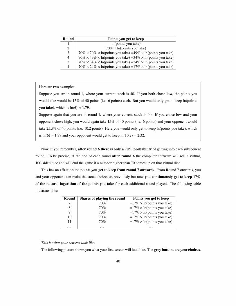
Anyway, the following table shows how this works. In round 1 you get to keep the natural logarithm of

the points you decide to take. In round 2 you get 70% of the natural logarithm of the points you take.

In round 3, you get to keep 70% of 70% of the natural logarithm of the points you took, and so on and so

forth. (Note that “ln” just means natural logarithm.)

39

Round Points you get to keep1 ln(points you take)2 70% × ln(points you take)3 70% × 70% × ln(points you take) =49% × ln(points you take)4 70% × 49% × ln(points you take) =34% × ln(points you take)5 70% × 34% × ln(points you take) =24% × ln(points you take)4 70% × 24% × ln(points you take) =17% × ln(points you take)

Here are two examples:

Suppose you are in round 1, where your current stock is 40. If you both chose low, the points you

would take would be 15% of 40 points (i.e. 6 points) each. But you would only get to keep ln(points

you take), which is ln(6) ≈ 1.79.

Suppose again that you are in round 1, where your current stock is 40. If you chose low and your

opponent chose high, you would again take 15% of 40 points (i.e. 6 points) and your opponent would

take 25.5% of 40 points (i.e. 10.2 points). Here you would only get to keep ln(points you take), which

is ln(6) ≈ 1.79 and your opponent would get to keep ln(10.2) = 2.32.

Now, if you remember, after round 6 there is only a 70% probability of getting into each subsequent

round. To be precise, at the end of each round after round 6 the computer software will roll a virtual,

100-sided dice and will end the game if a number higher than 70 comes up on that virtual dice.

This has an effect on the points you get to keep from round 7 onwards. From Round 7 onwards, you

and your opponent can make the same choices as previously but now you continuously get to keep 17%

of the natural logarithm of the points you take for each additional round played. The following table

illustrates this:

Round Shares of playing the round Points you get to keep7 70% =17% × ln(points you take)8 70% =17% × ln(points you take)9 70% =17% × ln(points you take)

10 70% =17% × ln(points you take)11 70% =17% × ln(points you take). . . . . . . . .

This is what your screens look like:

The following picture shows you what your first screen will look like. The grey buttons are your choices.

40

The purple boxes display the points you get to keep, the yellow boxes display the points your opponent

gets to keep. The little grey boxes show you what your next stock will be if you were to make that choice.

The big grey boxes show you what either player would get if you were to choose chance.

If you click a choice button, a red frame will appear around the choice that you have picked (see image).

If you click on the “chance” choice-button, a box will appear next to it. It tells you what the cost

of choosing chance would be, if you chose it in your current round. The following screenshot gives an

example:

Of course, you do not know what your opponent?s choice will be until the next round, so do not wait for

him/her.

At the bottom of the screen there is a red OK button. You ought to press it in order to confirm your

choice and enter the next round.

Finally, the following picture shows the screen you would get if either of you were to choose chance; it

shows you what chance mode looks like:

41

Stock:

Now, there is a little more to know about the stock of points. First, depending on the choices made, the

stock decreases in size. But second, it also replenishes. It regrows by 30% each round. This is how the next

stock of points is calculated:

42

1. Current stock - points you take - points opponent takes = remaining stock

2. Remaining stock + 30% = next stock

Here are two examples:

Suppose the current stock is 40 and you choose low and your opponent chooses high. Then we

calculate: (40 − 6 − 10.2) × 1.30 = 30.94 points.

Suppose the current stock is 40 and you choose low and your opponent chooses chance. Then we

calculate: (40 − 24 − 3.2 − 1.6) × 1.3 = 14.56 points. Here the 24 is the cost of playing chance, if you

remember from above.

This picture highlights your current stock and next stock if you choose low and if your opponent

chooses either high or chance:

This is it. Good luck!

43

References

[1] Klaus Abbink, Jordi Brandts, Benedikt Herrmann, and Henrik Orzen. Intergroup conflict and intra-

group punishment in an experimental contest game. American Economic Review, 100(1):420–447,

2010.

[2] Klaus Abbink and Thomas de Haan. Trust on the brink of armageddon: The first-strike game. European

Economic Review, 67:190–196, 2014.

[3] Olaf Bock, Ingmar Baetge, and Andreas Nicklisch. hroot: Hamburg registration and organization

online tool. European Economic Review, 71:117–120, 2014.

[4] Luis Cabral, Erkut Y. Ozbay, and Andrew Schotter. Intrinsic and instrumental reciprocity: An experi-

mental study. Games and Economic Behaviour, 87:100–121, 2014.

[5] Marco Casari and Charles Plott. Decentralized management of common property resources: Experi-

ments with a centuries-old institution. Journal of Economic Behavior & Organization, 51(2):217–247,

2003.

[6] Jonathan Cave. Long-term competition in a dynamic game: the cold fish war. RAND Journal of

Economics, 18 (4):596–610, 1987.

[7] Pedro Dal Bo. Cooperation under the shadow of the future: Experimental evidence from infinitely

repeated games. American Economic Review, 95(5):1591–1604, 2005.

[8] Pedro Dal Bo and Guillaume Frechette. The evolution of cooperation in infinitely repeated games:

Experimental evidence. American Economic Review, 101:411–429, 2011.

[9] Pedro Dal Bo and Guillaume Frechette. On the determinants of cooperation in infinitely repeated

games: A survey. Working Paper, 2014.

[10] Prajit K. Dutta. A folk theorem for stochastic games. Journal of Economic Theory, 66:1–32, 1995.

[11] Prajit K. Dutta and Roy Radner. A strategic analysis of global warming: Theory and some numbers.

Journal of Economic Behavior & Organization, 71:187–209, 2009.

[12] Catherine C. Eckel and Philip J. Grossman. Are women less selfish than men?: Evidence from dictator

experiments. Economic Journal, 108:726–735, 1998.

44

[13] Dan Kovenock Emmanuel Dechenaux and Roman M. Sheremeta. A survey of experimental research

on contests, all-pay auctions and tournaments. Experimental Economics, forthcoming, 2014.

[14] Ernst Fehr and Simon Gaechter. Cooperation and punishment in public goods experiments. American

Economic Review, 90(4):980–994, 2000.

[15] Robert Frank, Thomas Gilovich, and Denis T. Regan. Does studying economics inhibit cooperation?

Journal of Economic Perspectives, 7(2):159–171, 1993.

[16] Garrett Hardin. The tragedy of the commons. Science, 162:1243–1248, 1968.

[17] Luisa Herbst, Kai A. Konrad, and Florian Morath. Endogenous group formation in experimental con-

tests. European Economic Review, Forthcoming, 2015.

[18] Andrew Herr, Roy Gardner, and James M. Walker. An experimental study of time-independent and

time-dependent externalities in the commons. Games and Economic Behaviour, 19(1):77–96, 1997.

[19] Thomas F. Homer-Dixon. Environment, Scarcity, and Violence. Princeton University Press, 1999.

[20] Changxia Ke, Kai A. Konrad, and Florian Morath. Alliances in the shadow of conflict. Economic

Inquiry, 53(2):854–871, 2015.

[21] Juan A. Lacomba, Francisco Lagosa, Ernesto Reuben, and Frans van Winden. On the escalation and

de-escalation of conflict. Games and Economic Behaviour, 86:40–57, 2014.

[22] Michael McBride and Stergios Skaperdas. Conflict, settlement, and the shadow of the future. Journal

of Economic Behavior & Organization, 105:75–89, 2014.

[23] Thomas R. Palfrey and Howard Rosenthal. Repeated play, cooperation and coordination: an experi-

mental study. Review of Economic Studies, 61(3):545–565, 1994.

[24] Alvin E Roth and J.Keith Murnighan. Equilibrium behavior and repeated play of the prisoner’s

dilemma. Journal of Mathematical Psychology, 17(2):189–198, 1978.

[25] Petros G. Sekeris. The tragedy of the commons in a violent world. RAND Journal of Economics,

45(3):521–532, 2014.

[26] Gerhard Sorger. A dynamic common property resource problem with amenity value and extraction

costs. International Journal of Economic Theory, 1 (1):3–19, 2005.

45

[27] Nicholas Stern. Stern review on the economics of climate change. Cambridge University Press, 2007.

[28] Emanuel I. Vespa. An experimental investigation of strategies in dynamic games. mimeo, UC Santa

Barbara, 2014.

46

Date post:	13-Apr-2018
Category:	Documents
Upload:	vuonglien
View:	215 times
Download:	1 times

Can Violence Harm Cooperation? Experimental Evidence · Can Violence Harm Cooperation? Experimental...

Documents