Can We Prevent Boom-Bust Cycles During Euro Area Accession?

Open Econ Rev (2014) 25:35–69DOI 10.1007/s11079-013-9299-z

RESEARCH ARTICLE

Can We Prevent Boom-Bust Cycles During Euro AreaAccession?

Michał Brzoza-Brzezina ·Pascal Jacquinot ·Marcin Kolasa

Published online: 15 January 2014© Springer Science+Business Media New York 2014

Abstract Euro-area accession caused boom-bust cycles in several catching-up econ-omies. Declining interest rates and easier financing conditions fuelled spending andborrowing from abroad. Over time inflation deteriorated external competitiveness,turning the boom into a bust. We ask whether such a scenario can be avoidedusing macroeconomic tools that are available in the period of joining a monetaryunion: central parity revaluation, fiscal tightening or increased taxation. We find thatexchange rate revaluation is the most attractive option. It simultaneously trims theexpansion of output and domestic demand, reduces the cost pressure and ranks firstin terms of welfare.

Keywords Boom-bust cycles · Euro area accession · Dynamic general equilibriummodels

JEL Classifications E52 · E58 · E63

1 Introduction

Several countries witnessed a boom-bust cycle during their euro area accession. Thispattern was particularly pronounced in relatively poor, catching-up economies, where

M. Brzoza-Brzezina (�) · M. KolasaNarodowy Bank Polski and Warsaw School of Economics, Warsaw, Polande-mail: [email protected]

M. Kolasae-mail: [email protected]

P. JacquinotDirectorate General of Research, European Central Bank, Frankfurt, Germanye-mail: [email protected]

mailto:[email protected]



36 M. Brzoza-Brzezina et al.

nominal and real interest rates were relatively high before the monetary integration.One of the crucial features of a currency union is equalization of short-term interestrates as these are determined by the (now single) central bank. This means a sub-stantial reduction of these rates in high-growth economies. Medium and long-terminterest rates (e.g., on government bonds) need not be equal across the monetaryunion members. Nevertheless, in practice, they also tend to adjust substantially, themain reasons being elimination of the exchange rate risk and increased credibil-ity. Moreover, for a small economy, entering a monetary union means accessingan almost inexhaustible pool of funds, which facilitates financing borrowing needs.Finally, joining the club of more developed economies may be (rightly or wrongly)perceived as a permanent boost to productivity. All these developments induce agentsto borrow more and increase spending. As a result, the economy enters a boom phase,characterised by expansion of consumption, investment and credit.

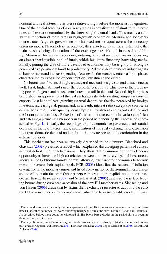
No boom lasts forever, though, and several mechanisms give an end to such one aswell. First, higher demand raises the domestic price level. This lowers the purchas-ing power of agents and hence contributes to a fall in demand. Second, higher pricesbring about an appreciation of the real exchange rate, deteriorating competitiveness ofexports. Last but not least, growing external debt raises the risk perceived by foreigninvestors, increasing risk premia and, as a result, interest rates (except the short-termcentral bank rate). Consequently, consumption, investment and exports decline andthe boom turns into bust. Behaviour of the main macroeconomic variables of richand catching-up euro area members in the period neighbouring their accession is pre-sented in Fig. 1.1 Clearly, the second group of economies experienced a substantialdecrease in the real interest rates, appreciation of the real exchange rate, expansionin output, domestic demand and credit to the private sector, and deterioration in theexternal position.

This mechanism has been extensively described in the literature. Blanchard andGiavazzi (2002) presented a model which explained the diverging patterns of currentaccount deficits in a monetary union. They show that a common currency offers anopportunity to break the high correlation between domestic savings and investment,known as the Feldstein-Horioka puzzle, allowing lower income economies to borrowmore to increase their capital stock. ECB (2003) identified the reasons of inflationdivergence in the monetary union and listed convergence of the nominal interest ratesas one of the main factors.2 Other papers were even more explicit about boom-bustcycles. Brzoza-Brzezina (2005) and Schadler et al. (2005) analysed the risk of lend-ing booms during euro area accession of the new EU member states. Siedschlag andvon Hagen (2006) argue that by fixing their exchange rate prior to adopting the eurothe EU new member states become more vulnerable to unsustainable capital inflows.

1These results are based not only on the experience of the official euro area members, but also of threenew EU member countries that were following hard pegs against the euro: Estonia, Latvia and Lithuania.As described below, these countries witnessed similar boom-bust episodes in the period close to peggingtheir currencies to the euro.2The large literature on inflation divergence in the euro area is also closely related to the topic of boom-bust cycles (Angeloni and Ehrmann 2007; Honohan and Lane 2003; Lopez-Salido et al. 2005; Zdarek andAldasoro 2009).

Can We Prevent Boom-Bust Cycles During Euro Area Accession? 37

(a) Real interest rate

-2%

-1%

0%

1%

2%

3%

-3 -2 -1 0 1 2 3 4

Rich Catching-up

(b) Real effective exchange rate (ULC)

85

90

95

100

105

-3 -2 -1 0 1 2 3 4Rich Catching-up

(c) Inflation

0%

2%

4%

6%

-2 -1 0 1 2 3 4

Rich Catching-up

(d) Loans

0

2

4

6

8

10

12

-3 -2 -1 0 1 2 3 4

Rich Catching-up

(e) Consumption

0%

2%

4%

6%

8%

10%


(f) GDP

0%

2%

4%

6%

8%

10%


(g) Current account balance

-12%

-10%

-8%

-6%

-4%

-2%

0%

2%

4%

-3 -2 -1 0 1 2 3 4

Rich Catching-up

(h) Net foreign assets

-80%

-60%

-40%

-20%

0%

20%

-3 -2 -1 0 1 2 3 4

Rich Catching-up

Fig. 1 Stylised facts for boom-bust cycles. The figures present unweighted averages of rich (Austria,Belgium, Finland, France, Germany, Italy and Netherlands) and catching-up (Estonia, Greece, Latvia,Lithuania, Portugal and Spain) euro area members and countries with a hard peg against the euro. Theplots are centred around the year (denoted as zero) of each country’s accession or pegging (Estonia - 1999,Latvia - 2004, Lithuania - 2002). We drop the observations that were substantially affected by factorsunrelated to these processes, e.g., the Russian crisis of 1998 and the financial crisis of 2008-09. Theseinclude i.a. GDP and consumption growth rates in Estonia and Lithuania in 1999 and all data for Latviain 2009. GDP and consumption are presented as growth rates, the current account balance and net foreignassets as percent of GDP, while loans as percentage point change of the ratio of loans to the private sectorto GDP. Inflation is measured with HICP excluding energy and seasonal food. The real effective exchangerate is deflated using unit labour costs (EA accession or pegging year = 100, increase denotes depreciation).Source: Eurostat, IFS and ESCB WGEM Report on empirical macro-financial linkages


Fagan and Gaspar (2007) documented the diverging patterns of main macroeconomicvariables (i.a. real interest rates, consumption, lending and current account balances)between the core and converging countries of the euro area. They presented a generalequilibrium framework based on Blanchard-Yari households that replicates the mainfeatures of the boom-bust scenario described above. Blanchard (2007) and Almeidaet al. (2009) analysed the case of Portugal and ascribed its boom-bust pattern to thedrop in interest rates related to the euro area accession, while Honohan and Leddin(2006) documented similar developments in Ireland. Eichengreen and Steiner (2008)analysed the potential of Poland to become a victim of the boom-bust scenario dur-ing the euro adoption. They found that several features (relatively high interest rates,low credit to GDP ratio) place Poland on the list of potentially endangered countries.As mentioned above, the list of countries already affected by a boom-bust scenario isnot restricted to official euro area members. Several new EU member states peggedtheir currencies to the euro. In particular, the three Baltic countries (Estonia, Latviaand Lithuania) experienced a dramatic overheating in the mid 2000s, with low inter-est rates imported from the euro area being one of the potential culprits (Brixiovaet al. 2009; Kuodis and Ramanauskas 2009). All in all, there is plenty of evidencethat the euro area accession of catching-up economies might end up in unsustainablebooms.

In this paper we ask whether such a boom in domestic demand can be pre-vented using tools that remain available to policymakers in the process of euroadoption and thereafter. We concentrate our attention on Poland, by far the biggestnew EU member country which is supposed to join the euro area in the future.At the same time, its GDP per capita amounts to approximately 60 % of the euroarea average and its interest rates are still substantially higher than in the euro area.As such, Poland is a model example of a potential boom-bust cycle victim. How-ever, the analysis presented in this paper also applies to other new EU memberstates.

Our simulations are based on EAGLE, a multicountry model developed by Gomeset al. (2012). Before doing them, however, we substantially modify the model andits calibration. First, the model is extended to allow for a non-zero import content ofexports. This feature, being relatively less important in the original setting of EAGLEthat was calibrated for Germany, the rest of the Euro Area, the United States andthe rest of the world, is highly relevant for the new EU member states, where theimport content of exports is relatively high. Second, we incorporate public goodsinto households’ utility function, which allows us to perform meaningful welfarecomparisons across alternative fiscal policies. Third, the calibration of the model ischanged so that it now includes Poland, the euro area, the United States and the restof the world.

After extending and recalibrating the model we design a series of simulations.Our baseline scenario consists of declining interest rates under a fixed exchange rateregime. This generates a boom, under which output expands by nearly 2.5 % abovethe steady state, consumption grows by 5 % and investment by above 12 %. As aconsequence, inflation increases, the real exchange rate appreciates and, after approx-imately two years, the boom turns into bust. We design four policy experiments thatare supposed to trim the boom-bust cycle. First, we consider a revaluation of the


exchange rate, a policy tool that is available only before joining the euro area. Sec-ond, we analyse the effects of increasing two tax rates: VAT and personal incometax (PIT). Finally, we experiment with cuts in government expenditures. To makeour scenarios more realistic, we impose implementability constraints on all policiesconsidered, i.e., we do not allow for repeated revaluations or changes in the fiscalparameters.

Our main findings are as follows. First, all considered policies are able to sub-stantially smooth the output boom. Second, the alternative policy interventions havedifferentiated effects on other macro variables. In particular, fiscal contraction addseven more to the private demand boom, a higher PIT rate increases inflation, whilea VAT hike increases the boom in investment. Overall, in this category, the exchangerate revaluation cuts off relatively well. Third, this policy ranks first when the model-consistent welfare criterion is applied. Two important robustness checks based onalternative mechanisms generating the boom-bust cycle do not change our main con-clusions. They also remain unaffected when we allow private agents to anticipate thedate of eurozone entry.

When comparing the size of instrument adjustment minimising the output gapvolatility, we find that the optimal revaluation amounts to ca. 7 %, the VAT rate shouldbe raised by 9 percentage points, the PIT rate by 12 percentage points and fiscalcontraction should amount to around 2 % of GDP. Thus, the analysed tax policies arenot only relatively inefficient in smoothing the output boom, but also very difficult toimplement from the political perspective. On the other hand, the fiscal contraction,and even more the exchange rate revaluation seem to be of acceptable magnitudes.Given these considerations, together with the results of the welfare analysis and theundesirable property of spending cuts which increase the consumption boom, we findthe exchange rate revaluation the most promising tool in smoothing out the boom-bust cycle.

Having said this, one thing should be made explicit. In this paper we deal withthe risk of a boom-bust cycle in domestic demand. One important issue that thisstudy does not take into account is the possible emergence and bursting of asset pricebubbles. EAGLE has a well developed structure of production, international linkagesand government policies, which seem important when analysing issues related tothe monetary union accession, exchange rate movements and policy intervention.However, this comes at a cost, being the model size. It seems hardly possible toextend such a model for the existence of asset price bubbles and regulatory policies.Second, we doubt whether policies available to the local authorities are able to stop anasset price bubble from emerging, due to potential regulatory arbitrage. Nevertheless,we believe that this is an important and interesting topic for further research.

The rest of the paper is structured as follows. In Section 2 we present the model, itscalibration and the main business cycle properties. Section 3 discusses our baselineboom-bust scenario. Section 4 describes how we define and design the optimal pol-icy interventions. The scenarios implied by these policies are presented in Section 5and evaluated in Section 6. Section 7 discusses robustness checks, based on threealternative boom-bust scenarios. Section 8 concludes.


2 The Model

2.1 EAGLE and its Extension

The EAGLE (Euro Area and GLobal Economy) model is a four-country dynamicstochastic general equilibrium (DSGE) model of the euro area in a global economy.It includes Germany, the rest of the euro area (which are both in a monetary union),the US and the rest of the world. EAGLE, based on the NAWM (Coenen et al. 2008),is also in the vein of the other international models such as GEM (Bayoumi et al.2004) or SIGMA (Erceg et al. 2006). Thus, the new open economy macroeconomicsparadigm constitutes its theoretical background. All country-bloc specifications areidentical.

Households are infinitely lived, consume final goods and supply labour to all firmsin a monopolistic manner. Wages are sticky a la Calvo with an indexation scheme.Households are distinguished according to their ability to access the financial market.Non-Ricardian agents that do not have this facility can only finance their consump-tion through labour income. At the opposite, Ricardian agents own domestic firms,rent the physical capital to them, and can buy or sell bonds: a government bond or abond denominated in US dollars. The internationally traded bond is subject to trans-action costs, meaning that households pay a premium to financial intermediaries.There are also adjustment costs on physical capital accumulation. Both capital andlabour are internationally immobile.

On the supply side, there are two types of firms. Firms producing final goods forconsumption or investment purposes use a constant elasticity of substitution (CES)technology assembling domestic intermediate goods and imports (that are subjectto adjustment costs) and act under perfect competition. Firms producing interme-diate goods operate under monopolistic competition. Intermediate goods can eitherbe internationally traded (tradable sector) or not (nontradable sector). Both sectorsuse a Cobb-Douglas production function combining domestic capital and domesticlabour. Exporting firms set prices in the currency of the destination market (local cur-rency pricing) to limit the exchange rate pass-through. Finally, staggered contracts ala Calvo (with indexation) introduce sluggishness in price adjustment.

The government purchases a public good (nontradable only) and finances itsexpenditure by issuing bonds and levying taxes. These taxes can either be lump-sumor distortionary, with the latter based on consumption purchases, labour, capital ordividend incomes. Fiscal authorities make transfers to households and earn seignior-age on outstanding money holdings. The fiscal rule sets the lump-sum tax bytargeting the debt-to-GDP ratio. Monetary authorities fix the short-term nominalinterest rates with a Taylor rule.

The original structure of the model has been amended to better fit the Polish econ-omy. In particular, the Polish economy features a much higher import content ofexports than for instance the euro area or the United States. This feature can be impor-tant while running simulations in which international linkages play an important role.For this reason we extend the model for the import content of exports. FollowingCoenen and Vetlov (2009), we introduce a new type of good, i.e., the export good,


which consists of domestic tradables and imported goods. This good is producedunder monopolistic competition and priced in the currency of the destination market.3

Another important modification of the original structure of EAGLE is related toour use of welfare as one of the criteria for evaluation of alternative policy inter-ventions. It is standard in the DSGE literature to include government purchasesneither in households’ utility nor firms’ production function. With such an assump-tion, however, public expenditures are wasteful and hence welfare can be increasedby driving them to zero. To eliminate such corner prescriptions in our welfare anal-ysis, we interpret government spending as provision of public goods and modify theutility function of each household type accordingly. Our aim is to make this modifi-cation as natural and neutral as possible. More specifically, the flow of governmentgoods is assumed to be equally distributed (in per capita terms) across Ricardianand non-Ricardian households. Further, we assume that utility is separable in privateconsumption and public goods so that no first order conditions of households’ opti-mization are affected by our modification. We also use the same functional formsfor the utility components related to both types of goods. Finally, we follow Adamand Billi (2008) and calibrate the relative weight on the utility component includinggovernment spending such that for each type of households the steady state marginalutility of public goods provision and private goods consumption are equalized.

2.2 Calibration

As already mentioned, we are interested in examining the impact of euro area acces-sion on a converging economy, and hence calibrate the model to Poland (PL), theeuro area (EA), the United States (US) and the rest of the world (RW). Our strategyto calibrate EAGLE can be divided into two stages. First, we pin down a subset ofparameters governing some key steady-state ratios, using their approximate empiri-cal counterparts. Next, we calibrate the remaining parameters of the model, drawingheavily on the original version of EAGLE, which in turn can be traced back to theparametrisation of the NAWM or GEM, as well as estimated small scale DSGE mod-els for the euro area (e.g., Smets and Wouters 2003; Adolfson et al. 2007; Christoffelet al. 2008), the United States (e.g., Christiano et al. 2005) and Poland (Grabek et al.2011; Kolasa 2009; Gradzewicz and Makarski 2013). The calibrated parameters arereported in Tables 1–7. Below we provide a brief discussion on our main choices anddata sources.

2.2.1 Steady-State Ratios

The relative size of each region is calibrated to reflect its GDP share in the worldeconomy. Consistently with the assumption that each region’s steady-state tradebalance is zero, we set the nominal output shares of consumption, governmentexpenditures and investment to the respective domestic demand shares of private

3Details of the derivation are given in the technical appendix available in the working paper version of thisarticle.


Table 1 Steady state ratios

PL EA US RW

GDP share in world GDP (%) 1.0 22.0 28.0 49.0Consumption share in GDP (%) 61.3 58.1 66.6 58.3Government expenditures share in GDP (%) 17.4 20.5 14.7 16.6Investment share in GDP (%) 21.2 21.4 18.7 25.1Imported consumption goods share in GDP (%) 11.3 8.2 7.7 3.6Imported investment goods share in GDP (%) 13.9 8.4 7.6 4.5

consumption, government consumption and gross capital formation. All this datacorresponds to the averages for the period 1995-2008 and comes from the nationalaccounts statistics collected in the Eurostat and World Development Indicatorsdatabases.

To obtain a more recent picture of international trade relations, we set the totalimport share of each region using the same data source, but averaged over a shortersample (2004-2008). The structure of bilateral trade flows, including their finaluse breakdown (consumption, investment or intermediate), relies on flows of goodsextracted from the CHELEM database and averaged over the years 2004-2008. Theexception is Poland, for which we were able to collect data on bilateral trade in bothgoods and services provided by the Narodowy Bank Polski. It is worth noting thatmore than half of Poland’s imports of any type of goods come from the euro area.

The shares of domestic tradables in production of the export good (i.e. one minusthe import content of exports) were set to 80 % for the EA, 85 % for the US, 55 % forPL and 65 % for the RW. For the former three regions this is consistent with estimates

Table 2 International linkages

to\from PL EA US RW

Consumption goodsPL – 52.1 2.9 45.0EA 4.4 – 7.8 87.8US 0.2 14.7 – 85.1RW 2.3 58.3 39.4 –

Investment goodsPL – 51.2 3.7 45.1EA 3.0 – 11.6 85.4US 0.2 14.9 – 84.9RW 1.0 47.0 52.0 –

Intermediate goodsPL – 51.5 2.3 46.2EA 3.4 – 6.0 90.7US 0.2 11.7 – 88.1RW 1.6 45.3 53.1 –

Note: the numbers refer to percentage shares of imports from column country to row country in totalimports to row country of consumption, investment or intermediate goods, respectively


Table 3 Final goods

PL EA US RW

Quasi-share of nontradables in final consumption goods (%) 65.0 65.0 65.0 65.0Quasi-share of nontradables in final investment goods (%) 25.0 25.0 25.0 25.0Quasi-share of imports in export good (%) 45.0 20.0 15.0 35.0Quasi-share of imports in tradable consumption goods (%) 66.1 44.3 40.4 17.3Quasi-share of imports in tradable investment goods (%) 90.9 56.1 60.4 23.0Elasticity of substitution between tradable and nontradable goods 0.5 0.5 0.5 0.5Elasticity of substitution between domestic goods and imports

(production of consumption and investment goods) 2.5 2.5 2.5 2.5Elasticity of substitution between domestic goods and imports

(production of export good) 1.5 1.5 1.5 1.5Elasticity of substitution between imported goods 2.5 2.5 2.5 2.5

from the input/output matrices, while for the RW it is based on the proportion ofintermediate goods imports to total exports (no input/output matrix is available). Thequasi-shares of nontradables in the consumption and investment baskets are set to75 % and 35 %, respectively, which together with the assumption of fully nontradablecontent of government expenditures implies the share of tradable output in GDP ofabout 35 %. This number is roughly consistent with the values implied by the shareof agriculture, mining and manufacturing in the total market economy, calculatedfor Poland, the euro area and the United States for the period 1995-2008 using theEU-KLEMS database.

2.2.2 Other Parameters

We set the capital share in production functions in all countries to 30 %. The taxstructure for the euro area and the United States is taken directly from Gomes et al.(2012). The tax structure for Poland comes from national sources and tax wedges forthe rest of the world are calibrated at the US level. The capital tax rate is treated as afree parameter and used to calibrate the region-specific investment shares in output.

Table 4 Intermediate goods

PL EA US RW

Capital share in nontradable production 0.30 0.30 0.30 0.30

Capital share in tradable production 0.30 0.30 0.30 0.30

Elasticity of substitution between intermediate nontradable varieties 3.0 3.0 4.3 4.3

Elasticity of substitution between intermediate tradable varieties 4.3 4.3 6.0 6.0

Elasticity of substitution between imported varieties 4.3 4.3 6.0 6.0

Calvo probability for goods sold domestically 0.75 0.75 0.75 0.75

Calvo probability for exported goods 0.75 0.75 0.75 0.75

Price indexation 0.50 0.50 0.50 0.50


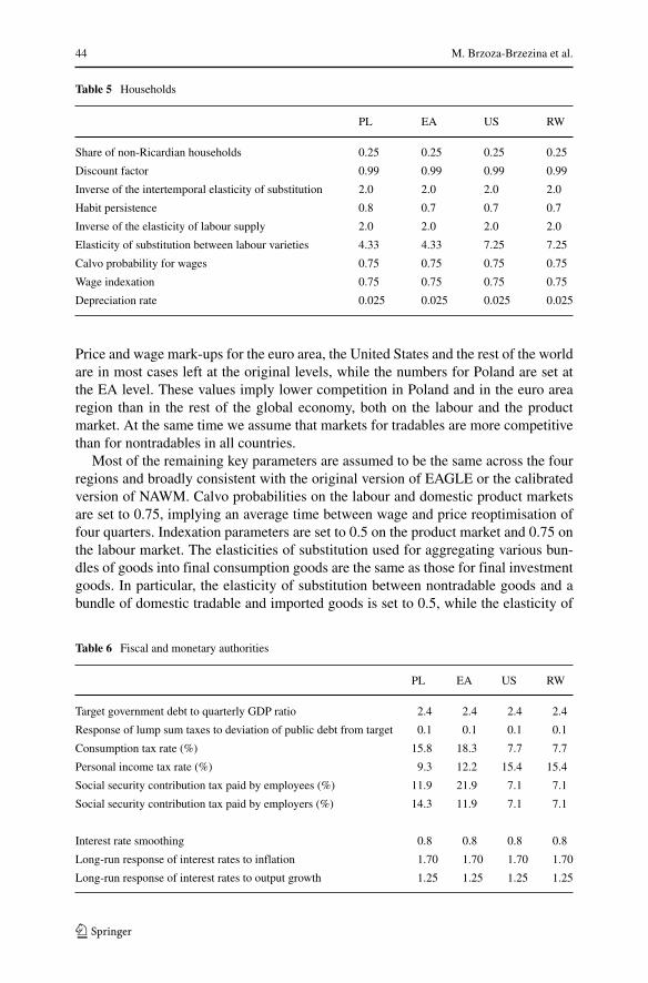
Table 5 Households

PL EA US RW

Share of non-Ricardian households 0.25 0.25 0.25 0.25

Discount factor 0.99 0.99 0.99 0.99

Inverse of the intertemporal elasticity of substitution 2.0 2.0 2.0 2.0

Habit persistence 0.8 0.7 0.7 0.7

Inverse of the elasticity of labour supply 2.0 2.0 2.0 2.0

Elasticity of substitution between labour varieties 4.33 4.33 7.25 7.25

Calvo probability for wages 0.75 0.75 0.75 0.75

Wage indexation 0.75 0.75 0.75 0.75

Depreciation rate 0.025 0.025 0.025 0.025

Price and wage mark-ups for the euro area, the United States and the rest of the worldare in most cases left at the original levels, while the numbers for Poland are set atthe EA level. These values imply lower competition in Poland and in the euro arearegion than in the rest of the global economy, both on the labour and the productmarket. At the same time we assume that markets for tradables are more competitivethan for nontradables in all countries.

Most of the remaining key parameters are assumed to be the same across the fourregions and broadly consistent with the original version of EAGLE or the calibratedversion of NAWM. Calvo probabilities on the labour and domestic product marketsare set to 0.75, implying an average time between wage and price reoptimisation offour quarters. Indexation parameters are set to 0.5 on the product market and 0.75 onthe labour market. The elasticities of substitution used for aggregating various bun-dles of goods into final consumption goods are the same as those for final investmentgoods. In particular, the elasticity of substitution between nontradable goods and abundle of domestic tradable and imported goods is set to 0.5, while the elasticity of

Table 6 Fiscal and monetary authorities

PL EA US RW

Target government debt to quarterly GDP ratio 2.4 2.4 2.4 2.4

Response of lump sum taxes to deviation of public debt from target 0.1 0.1 0.1 0.1

Consumption tax rate (%) 15.8 18.3 7.7 7.7

Personal income tax rate (%) 9.3 12.2 15.4 15.4

Social security contribution tax paid by employees (%) 11.9 21.9 7.1 7.1

Social security contribution tax paid by employers (%) 14.3 11.9 7.1 7.1

Interest rate smoothing 0.8 0.8 0.8 0.8

Long-run response of interest rates to inflation 1.70 1.70 1.70 1.70

Long-run response of interest rates to output growth 1.25 1.25 1.25 1.25


Table 7 Adjustment costs

PL EA US RW

Capacity utilisation cost 2000 2000 2000 2000

Investment adjustment cost 6.0 6.0 6.0 6.0

Import adjustment cost for consumption goods 5.0 5.0 5.0 5.0

Import adjustment cost for investment goods 2.0 2.0 2.0 2.0

Import adjustment cost for intermediate goods 2.0 2.0 2.0 2.0

International transaction cost 0.0025 0.0025 – 0.0025

substitution between home-made and imported tradable baskets is calibrated at 2.5.The elasticity of substitution between domestic and imported goods in the productionof export goods is set at a somewhat lower level of 1.5 and the parameter governingsubstitutability across imports from different countries is assumed to be 2.5.

The choices of adjustment cost parameters are taken directly from the originalversions of EAGLE and NAWM as well. The response of the share of lump-sumtaxes in nominal output to deviations of the public debt-to-output ratio from the tar-get (60 % on an annual basis) is set to 0.1. We also maintain the NAWM assumptionon asymmetric distribution of lump sum transfers and taxes across the two typesof households, favouring those with limited access to capital markets in the propor-tion of 3 to 1. Finally, the long-run monetary policy response to inflation and outputgrowth is calibrated at 1.7 and 1.25, respectively, while the weight on the laggedinterest rate is set to 0.8.

Besides taking most parameters from the literature, we pay special attention tothe short-term dynamic responses of the Polish economy to various shocks. This iscrucial, taking into account the simulations to be performed. In particular, our goalwas to bring the impulse response functions close to those from the estimated DSGEmodels of the Polish economy (Grabek et al. 2011; Kolasa 2009; Gradzewicz andMakarski 2013). In order to match the impulse responses, we run the model assumingindependent monetary policy for Poland, as is currently the case. Given the calibra-tion presented above, this did not require substantial changes to the parameters, anexception being a somewhat higher habit persistence parameter, helping to trim thevolatility of consumption. The impulse response functions are presented in the nextsection.

2.3 Dynamic Properties

In this section we document the main dynamic properties of the recalibrated model.We concentrate on the reaction of the Polish economy to a set of standard shocks.4

As mentioned in the previous section, the calibration of several parameters was done

4For the sake of comparability with other studies, we calibrate the autoregressive coefficients of all shockprocesses at a common value of 0.9 and normalize the innovations size to 1 %.


0 10 20 30 400

0.2

0.4

0.6

0.8

1Output

0 10 20 30 400

0.2

0.4

0.6

0.8Consumption

0 10 20 30 40−0.2

0

0.2

0.4

0.6

0.8

1

1.2Investment

0 10 20 30 400

0.2

0.4

0.6

0.8Exports

0 10 20 30 40−0.2

−0.1

0

0.1

0.2

0.3

0.4

0.5Imports

0 10 20 30 400

0.02

0.04

0.06

0.08

0.1Gov. spending

0 10 20 30 40−0.2

0

0.2

0.4

0.6

0.8

1

1.2Real effective exchange rate

0 10 20 30 40−1.5

−1

−0.5

0

0.5Inflation

0 10 20 30 40−0.6

−0.5

−0.4

−0.3

−0.2

−0.1

0

0.1Interest rate

Fig. 2 Impulse responses to a technology shock. Solid line - peg, dashed line - independent monetarypolicy. Both responses for Poland. All values in per cent deviations from steady state except inflation andinterest rate, which are given in annualised percentage point deviations

so as to match the impulse responses to those from estimated DSGE models underthe assumption of independent monetary policy. On the other hand, our boom-bustscenarios will be designed under the assumption of a fixed exchange rate against theeuro. As a consequence, we present impulse responses under both monetary policyregimes.

Our analysis begins with the reaction to a standard technology shock, affectingto the same degree productivity in the tradable and nontradable sectors. Figure 2shows the reaction of the main macroeconomic variables. The impulse responses arestandard to a supply side shock. In particular, real variables increase while inflationdeclines. Under independent monetary policy, the central bank reacts to this by low-ering interest rates. However, this reaction is muted since output and inflation movein opposite directions. Under the fixed exchange rate regime, domestic interest ratesdecline slightly as well due to improvement in the current account balance, the result-ing lower risk premium and spillovers to the euro area. Given the weak reaction ofthe domestic central bank in the float case, the economy reacts similarly under bothexchange rate regimes.

Monetary policy shocks constitute a more interesting case (Fig. 3). Since underthe peg regime domestic monetary policy does not control the short-term interest


0 10 20 30 40−0.25

−0.2

−0.15

−0.1

−0.05

0

0.05

0.1Output

0 10 20 30 40−0.35

−0.3

−0.25

−0.2

−0.15

−0.1

−0.05

0Consumption

0 10 20 30 40−0.4

−0.3

−0.2

−0.1

0

0.1Investment

0 10 20 30 40−0.2

−0.15

−0.1

−0.05

0

0.05Exports

0 10 20 30 40−0.25

−0.2

−0.15

−0.1

−0.05

0

0.05

0.1Imports

0 10 20 30 40−10

−8

−6

−4

−2

0

2

4x 10

−3 Gov. spending

0 10 20 30 40−1

−0.8

−0.6

−0.4

−0.2

0

0.2


0 10 20 30 40−0.3

−0.25

−0.2

−0.15

−0.1

−0.05

0

0.05Inflation

0 10 20 30 40−0.2

0

0.2

0.4

0.6

0.8

1

1.2Interest rate

Fig. 3 Impulse responses to a monetary policy shock. Solid line - peg, dashed line - independent monetarypolicy. Both responses for Poland. All values in per cent deviations from steady state except inflation andinterest rate, which are given in annualised percentage point deviations

rate, in this case we present the reaction to a shock to the euro area interest rate. Thisshould be kept in mind since the euro area interest rate affects also the euro area econ-omy and so has an additional, indirect impact on Poland. In general, the shape of thereaction functions is standard. Output, consumption and investment decline, so doesinflation. The magnitude of reactions of the main variables under independent mone-tary policy is broadly consistent with that from other studies on the Polish economy.However, reactions under the peg are somewhat weaker. The reason is the exchangerate channel, which is an important component of the monetary transmission underthe float. After pegging to the euro, the appreciation of the real effective exchangerate is weaker and so is the reaction of most variables.

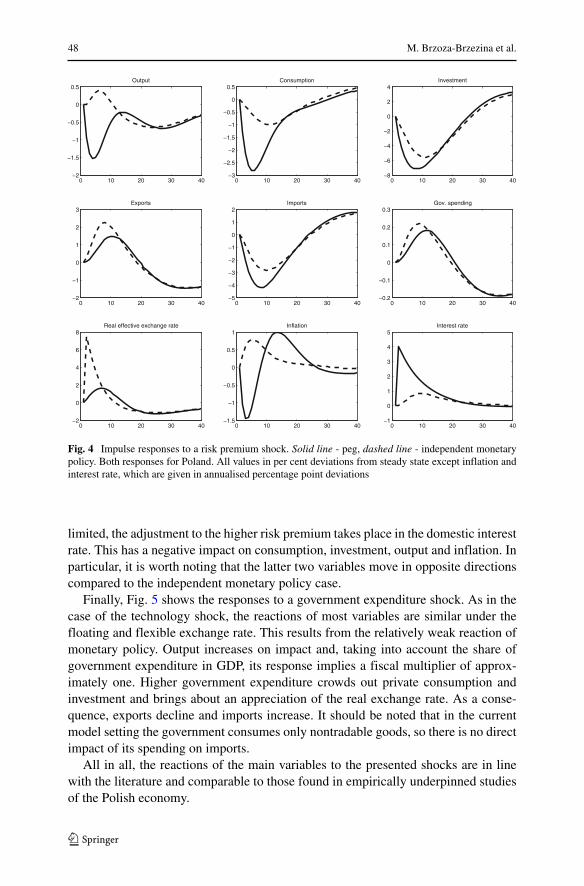
Figure 4 presents the impulse responses to a risk premium shock. The reactionunder the floating exchange rate comes primarily from the sharp depreciation ofthe exchange rate. As a result, exports surge and imports decline, generating a sur-plus in the current account and giving a boost to GDP. Following the exchange ratedepreciation, inflation increases, which results in a monetary policy tightening. Thiscontributes to a drop of consumption and investment. As before, the magnitude ofreaction of the main variables is in line with other estimates for Poland. The trans-mission pattern is different under the peg. Since the possible exchange rate reaction is


0 10 20 30 40−2

−1.5

−1

−0.5

0

0.5Output

0 10 20 30 40−3

−2.5

−2

−1.5

−1

−0.5

0

0.5Consumption

0 10 20 30 40−8

−6

−4

−2

0

2

4Investment

0 10 20 30 40−2

−1

0

1

2

3Exports

0 10 20 30 40−5

−4

−3

−2

−1

0

1

2Imports

0 10 20 30 40−0.2

−0.1

0

0.1

0.2

0.3Gov. spending

0 10 20 30 40−2

0

2

4

6

8Real effective exchange rate

0 10 20 30 40−1.5

−1

−0.5

0

0.5

1Inflation

0 10 20 30 40−1

0

1

2

3

4

5Interest rate

Fig. 4 Impulse responses to a risk premium shock. Solid line - peg, dashed line - independent monetarypolicy. Both responses for Poland. All values in per cent deviations from steady state except inflation andinterest rate, which are given in annualised percentage point deviations

limited, the adjustment to the higher risk premium takes place in the domestic interestrate. This has a negative impact on consumption, investment, output and inflation. Inparticular, it is worth noting that the latter two variables move in opposite directionscompared to the independent monetary policy case.

Finally, Fig. 5 shows the responses to a government expenditure shock. As in thecase of the technology shock, the reactions of most variables are similar under thefloating and flexible exchange rate. This results from the relatively weak reaction ofmonetary policy. Output increases on impact and, taking into account the share ofgovernment expenditure in GDP, its response implies a fiscal multiplier of approx-imately one. Higher government expenditure crowds out private consumption andinvestment and brings about an appreciation of the real exchange rate. As a conse-quence, exports decline and imports increase. It should be noted that in the currentmodel setting the government consumes only nontradable goods, so there is no directimpact of its spending on imports.

All in all, the reactions of the main variables to the presented shocks are in linewith the literature and comparable to those found in empirically underpinned studiesof the Polish economy.


0 10 20 30 400

0.2

0.4

0.6

0.8

1Output

0 10 20 30 40−0.35

−0.3

−0.25

−0.2

−0.15

−0.1

−0.05

0Consumption

0 10 20 30 40−0.15

−0.1

−0.05

0

0.05Investment

0 10 20 30 40−0.3

−0.25

−0.2

−0.15

−0.1

−0.05

0

0.05Exports

0 10 20 30 40−0.1

−0.05

0

0.05

0.1Imports

0 10 20 30 400

1

2

3

4

5

6Gov. spending

0 10 20 30 40−0.4

−0.3

−0.2

−0.1

0


0 10 20 30 40−0.2

−0.1

0

0.1

0.2

0.3

0.4

0.5Inflation

0 10 20 30 40−0.05

0

0.05

0.1

0.15

0.2

0.25

0.3Interest rate

Fig. 5 Impulse responses to a government expenditure shock. Solid line - peg, dashed line - independentmonetary policy. Both responses for Poland. All values in per cent deviations from steady state exceptinflation and interest rate, which are given in annualised percentage point deviations

3 Interest Rate Convergence

Entering the euro area has important implications for interest rate convergence. Sincemonetary policy is now conducted by a common central bank, short-term interestrates, being the bank’s instrument, must converge fully. The problem is more nuancedas regards long-term rates. Joining the common currency area necessarily eliminatesthe exchange rate risk premium and hence can be expected to lower these rates aswell. Moreover, if adopting the euro is perceived as a boost to credibility, it canalso reduce the default risk premium. Indeed, in the early years of the euro almostcomplete convergence of long-term yields between member countries suggested thatboth factors were at play. However, the strong divergence of long-term interest ratesthat could be observed after the financial crisis casts doubts whether the effect ofdefault risk reduction should be expected once Poland adopts the euro.

Accordingly, for our baseline scenario we make the following assumptions. Uponentry short-term interest rates converge completely. Given the historical experi-ence (2005-2011 average), we assume that short-term interest rates in Poland willdrop by 250 basis points. Regarding long-term interest rates, we assume that onlythe exchange rate risk will be eliminated, while default risk remains unchanged.


This implies reducing long-term rates by around 120 basis points, which corre-sponds to the historical (2005-2011) difference between the yields on 10-year Polishgovernment bonds denominated in Polish zlotys and euros.

Since there is only one interest rate in EAGLE, we proceed as follows. Consis-tently with the expectations hypothesis of the term structure of interest rates, wedefine the 10-year interest rate as the average of short term rates over the 40-quarterhorizon. The drop of the short term rate is driven by a positive risk premium shock,whose size and autoregressive coefficient are calibrated such that our assumptions onshort and long-term interest rate convergence are met simultaneously.

The dynamic responses to the baseline boom scenario are presented in Fig. 6.Lower interest rates make Ricardian households increase their spending, so con-sumption and investment go up. Higher demand leads to an expansion in domesticoutput and imports, so the current account balance deteriorates significantly. Theboom increases labour demand and improves the fiscal balance, which allows thegovernment following the fiscal rule to cut lump sum taxes. As a result, income ofnon-Ricardian households improves and their spending grows. Increased cost pres-sure pushes prices up. As the nominal exchange rate is fixed and prices abroad hardlymove, the real exchange rate appreciates.

0 20 40 60 80 100−0.5

0

0.5

1

1.5

2

2.5Output

0 20 40 60 80 100−2

−1

0

1

2

3

4

5Consumption

0 20 40 60 80 100−5

0

5

10

15Investment

0 20 40 60 80 100−1

0

1

2

3

4

5Fiscal surplus

0 20 40 60 80 100−3.5

−3

−2.5

−2

−1.5

−1

−0.5

0Current account balance

0 20 40 60 80 100−4

−3

−2

−1

0

1


0 20 40 60 80 100−2

−1

0

1

2

3Inflation

0 20 40 60 80 100−3

−2.5

−2

−1.5

−1

−0.5

0

0.5Interest rate

0 20 40 60 80 100−0.04

−0.03

−0.02

−0.01

0

0.01

0.02Euro area output

Fig. 6 Interest rate convergence scenario (baseline). The fiscal surplus and current account balance areexpressed relative to nominal output. Inflation and the nominal interest rate are annualised. All variablesare reported as per cent or percentage point deviations from their steady state values


This process initiates the bust phase of the cycle. Reduced competitiveness under-mines exports, which translates into lower output - the boom turns into bust alreadyafter approximately two years. Only once the cost pressures decline somewhat andthe competitiveness is restored do exports recover, which together with decliningimports leads to a second, but smaller in magnitude, expansion in output.

As Poland is a small country, the spillovers to other regions, even to the closelylinked euro area, are very limited. Since increased lending to Poland is financed withhigher savings of other regions, including the euro area, our scenario implies a verysmall contraction in the latter’s output. All in all, we believe that the designed sce-nario reflects the main feature of the boom-bust cycles described in the Introduction.We are now ready to analyse the effects of policies that could potentially cool downthe boom, and hence reduce the risk of a bust.

4 Designing Policies for the Boom

The model we are using is not able to capture all channels making the boom-bustcycle harmful. In particular, our baseline scenario is not a typical bubble, result-ing from overly optimistic expectations. Instead, it reflects dynamic responses ofrational agents, subject to a set of constraints. Since the model includes a range ofnominal and real rigidities, appropriately designed stabilization policies can be wel-fare improving. However, gains from applying them are known to be rather smallin a standard quantitative business cycle framework, at least when model-consistentevaluation criteria are used (Lucas 2003).

That said, one can list several reasons why smoothing the boom-bust cycle mightbe in practice more justified than the welfare analysis suggests. The most importantone is that temporary but prolonged periods of prosperity can lead to excessive opti-mism, increasing the likelihood of bubbles building up and making the necessaryadjustment of imbalances sudden and painful. Moreover, rapid expansions in outputand consumption are usually accompanied by lending booms, which may have detri-mental effects on the banking sector stability. Therefore, even though such effects arenot incorporated in our workhorse model, it still might be relevant to analyse whichpolicies are most successful in smoothing the boom.

For a small economy, adopting the euro means in practice giving up monetaryautonomy as short-term interest rates are now set by the European Central Bank inresponse to area-wide developments. The only monetary parameter that can be used(but only prior to accession) is revaluation of the nominal exchange rate. In contrast,the new entrant can still use a full set of fiscal instruments. In theory, one can designmany revenue and expenditure policies smoothing the boom completely. In practice,they would require changes of the fiscal instruments on a quarterly basis. While thismight be feasible for some types of expenditures, it is difficult to imagine so frequentadjustments in such parameters as the tax rates or major spending components.

Therefore, we restrict our attention to those policies that can be considered imple-mentable. In particular, we assume that the exchange rate can be revalued only once,and the tax rates can be changed twice (i.e., up and back to the original level) for


full-year periods. We make a similar assumption for the government spending sharein GDP, but additionally look at a variant allowing it to be adjusted every period.

For the reasons discussed before, we parametrize and evaluate alternative policiesusing two criteria. First, we consider a simple stabilization objective. While thereare a number of economic indicators that could be used as potential targets for acountercyclical policy, we use the most natural one, i.e., the output gap volatility,defined as the root mean square deviation of output from its steady state level andcalculated over a 10-year horizon. Even though the focus on output gap stabilizationseems natural given the common practice, this choice might be considered somewhatarbitrary. Therefore, we will also discuss the implications of the policies designed tominimise output gap volatility for other variables.

Second, we apply the welfare criterion. This is not straightforward as the steadystate equilibrium in the model is not efficient and so the constrained optimal policieswe consider imply non-zero interventions even if the interest rate convergence doesnot occur. Since we want to net such effects out, we proceed as follows. For eachpolicy variant, we calculate the optimal change of policy parameters with and withoutthe boom and define the best response to the boom from the welfare perspective asthe difference between the two. Essentially, this tells us how, taking the steady stateas the reference point, the optimal policy should be modified if faced with the boomscenario.

5 Policy Simulations

5.1 Exchange Rate Revaluation

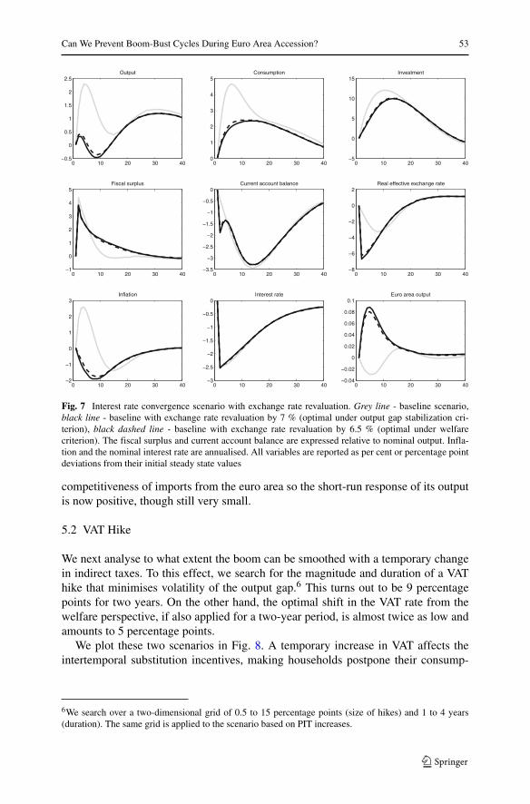
The first policy scenario we consider relies on counteracting the boom with a one-offexchange rate revaluation. One can think of this policy as resulting from an agree-ment between the new entrant and the rest of the euro area to set the conversion rateat a stronger level than currently prevailing on the foreign exchange market. Interest-ingly, the magnitude of the revaluation minimising the output gap volatility almostcoincides with that implied by the welfare criterion, amounting respectively to 7 %and 6.5 %.5

The dynamic responses to this scenario are plotted in Fig. 7. The exchange raterevaluation turns out quite successful in cooling down the boom. Compared to thebaseline, the initial swing in output is dramatically reduced. This affects house-holds’ income, so the peak response of consumption and investment is delayed anddecreased substantially. The contraction in exports is slightly deeper (by 0.7 percent-age points) than under baseline so the current account deteriorates more, but only inthe short run. The revaluation has also an effect on inflation, which is smoother andof different sign compared to the baseline. The stronger exchange rate increases price

5Since the parametrization of our policies is based on a grid search, the accuracy of our results is deter-mined by the size of the search step, which we set to 0.5 percentage points for all policies considered inthis section.


0 10 20 30 40−0.5

0

0.5

1

1.5

2

2.5Output

0 10 20 30 400

1

2

3

4

5Consumption

0 10 20 30 40−5

0

5

10

15Investment

0 10 20 30 40−1

0

1

2

3

4

5Fiscal surplus

0 10 20 30 40−3.5

−3

−2.5

−2

−1.5

−1

−0.5


0 10 20 30 40−8

−6

−4

−2

0


0 10 20 30 40−2

−1

0

1

2

3Inflation

0 10 20 30 40−3

−2.5

−2

−1.5

−1

−0.5

0Interest rate

0 10 20 30 40−0.04

−0.02

0

0.02

0.04

0.06

0.08

0.1Euro area output

Fig. 7 Interest rate convergence scenario with exchange rate revaluation. Grey line - baseline scenario,black line - baseline with exchange rate revaluation by 7 % (optimal under output gap stabilization cri-terion), black dashed line - baseline with exchange rate revaluation by 6.5 % (optimal under welfarecriterion). The fiscal surplus and current account balance are expressed relative to nominal output. Infla-tion and the nominal interest rate are annualised. All variables are reported as per cent or percentage pointdeviations from their initial steady state values

competitiveness of imports from the euro area so the short-run response of its outputis now positive, though still very small.

5.2 VAT Hike

We next analyse to what extent the boom can be smoothed with a temporary changein indirect taxes. To this effect, we search for the magnitude and duration of a VAThike that minimises volatility of the output gap.6 This turns out to be 9 percentagepoints for two years. On the other hand, the optimal shift in the VAT rate from thewelfare perspective, if also applied for a two-year period, is almost twice as low andamounts to 5 percentage points.

We plot these two scenarios in Fig. 8. A temporary increase in VAT affects theintertemporal substitution incentives, making households postpone their consump-

6We search over a two-dimensional grid of 0.5 to 15 percentage points (size of hikes) and 1 to 4 years(duration). The same grid is applied to the scenario based on PIT increases.


0 10 20 30 40−1

−0.5

0

0.5

1

1.5

2

2.5Output

0 10 20 30 40−1

0

1

2

3

4

5Consumption

0 10 20 30 40−5

0

5

10

15Investment

0 10 20 30 40−2

0

2

4

6

8

10Fiscal surplus

0 10 20 30 40−3.5

−3

−2.5

−2

−1.5

−1

−0.5


0 10 20 30 40−4

−3

−2

−1

0

1


0 10 20 30 40−2

−1

0

1

2

3Inflation

0 10 20 30 40−2.5

−2

−1.5

−1

−0.5

0Interest rate

0 10 20 30 40−0.04

−0.03

−0.02

−0.01

0

0.01


Fig. 8 Interest rate convergence scenario with a 2-year VAT hike. Grey line - baseline scenario, black solidline - baseline with VAT rate hike by 9 pp for 2 years (optimal under output gap stabilization criterion),black dashed line - baseline with VAT rate hike by 5 pp for 2 years (optimal under welfare criterion).The fiscal surplus and current account balance are expressed relative to nominal output. Inflation and thenominal interest rate are annualised. All variables are reported as per cent or percentage point deviationsfrom their initial steady state values

tion decisions. As a result, the short-run increase in consumption is nearly elimi-nated if the rate goes up by 9 percentage points and substantially decreased if thechange amounts 5 percentage points. However, in the former variant, once the taxrate is restored to its initial value, consumption expenditures quickly take off and inthe medium run reach values exceeding those under the baseline. Given the smooth-ing motive implied by households’ utility function, such swings in consumption areundesired and the welfare consistent criterion takes this into account. Since any VAThike makes the relative price of investment goods cheaper, the boom in investment ismagnified. Overall, the VAT policy successfully weakens the short run expansion indomestic demand, smoothing the boom in output and slightly decreasing the pace ofcurrent account deterioration. Inflation pressure, measured with the consumer priceindex at producer prices, is also reduced.7

7Naturally, with a hike in VAT, market prices of consumption goods go up much more compared to thebaseline scenario.


0 10 20 30 40−1

−0.5

0

0.5

1

1.5

2

2.5Output

0 10 20 30 400

1

2

3

4

5Consumption

0 10 20 30 40−5

0

5

10

15Investment

0 10 20 30 40−5

0

5

10

15Fiscal surplus

0 10 20 30 40−4

−3

−2

−1


0 10 20 30 40−5

−4

−3

−2

−1

0

1


0 10 20 30 40−3

−2

−1

0

1

2

3

4Inflation

0 10 20 30 40−2.5

−2

−1.5

−1

−0.5

0Interest rate

0 10 20 30 40−0.06

−0.04

−0.02

0

0.02


Fig. 9 Interest rate convergence scenario with a 2-year PIT hike. Grey line - baseline scenario, black solidline - baseline with PIT rate hike by 12 pp for 2 years (optimal under output gap stabilization criterion),black dashed line - baseline with PIT rate reduction by 0.06 pp for 2 years (optimal under welfare crite-rion). The fiscal surplus and current account balance are expressed relative to nominal output. Inflationand the nominal interest rate are annualised. All variables are reported as per cent or percentage pointdeviations from their initial steady state values

5.3 PIT Hike

If the government wants to minimise output volatility by changing personal incometaxes levied on labour income, it should increase the PIT rate by 12 percentagepoints for two years. In contrast, the welfare analysis prescribes virtually the samemagnitude of intervention with and without the boom.

Figure 9 helps to understand this result. As can be seen, increasing the PIT rate isquite effective in stifling domestic demand. In particular, it cools down the boom inboth consumption and investment. However, an increase in direct taxes decreases fac-tor supply, hence firms’ costs and inflation go up. This is costly in terms of welfare ifprices are set in a staggered fashion. Also, increased cost pressure erodes firms’ com-petitiveness. As a result, the real exchange rate appreciation is stronger and exportsfall by more than under the baseline. Finally, while a PIT hike helps to cut the peakresponse of output, it also makes the subsequent bust larger.


0 10 20 30 40−1

−0.5

0

0.5

1

1.5

2

2.5Output

0 10 20 30 400

1

2

3

4

5

6

7Consumption

0 10 20 30 40−5

0

5

10

15Investment

0 10 20 30 40−2

0

2

4

6

8Fiscal surplus

0 10 20 30 40−3.5

−3

−2.5

−2

−1.5

−1

−0.5


0 10 20 30 40−4

−3

−2

−1

0

1


0 10 20 30 40−2

−1

0

1

2

3Inflation

0 10 20 30 40−2.5

−2

−1.5

−1

−0.5

0Interest rate

0 10 20 30 40−0.04

−0.03

−0.02

−0.01

0

0.01


Fig. 10 Interest rate convergence scenario with government spending cuts. Grey line - baseline scenario,black solid line - baseline with fiscal contraction by 2 % of GDP for 3 years (optimal under output gapstabilization criterion), black dashed line - baseline with fiscal contraction by 0.04 % of GDP for 3 years(optimal under welfare criterion), black dotted line - baseline with government spending adjustments thatfully stabilize output. The fiscal surplus and current account balance are expressed relative to nominaloutput. Inflation and the nominal interest rate are annualised. All variables are reported as per cent orpercentage point deviations from their initial steady state values

5.4 Government Spending Cuts

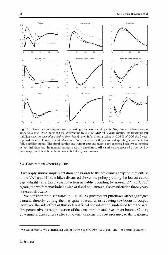
If we apply similar implementation constraints to the government expenditure cuts asto the VAT and PIT rate hikes discussed above, the policy yielding the lowest outputgap volatility is a three year reduction in public spending by around 2 % of GDP.8

Again, the welfare maximizing size of fiscal adjustment, also restricted to three years,is essentially zero.

We consider these scenarios in Fig. 10. As government purchases affect aggregatedemand directly, cutting them is quite successful in reducing the boom in output.However, the side effect of thus defined fiscal consolidation, undesired from the wel-fare perspective, is magnification of the consumption and investment booms. Cuttinggovernment expenditures also somewhat weakens the cost pressure, so the responses

8We search over a two-dimensional grid of 0.5 to 5 % of GDP (size of cuts) and 1 to 4 years (duration).


of inflation, the real exchange rate and hence the current account balance becomesmoother.

It can be argued that public spending is to a large extent at the discretion of thegovernment and so faces less severe implementation lags compared to changes in thetax rates. Therefore, one can at least conceptually think of a policy that fine-tunes thegovernment purchases so that output fluctuations are eliminated completely. Such apolicy is illustrated with dotted lines in Fig. 10. The required path of governmentexpenditures (not shown) is roughly the rescaled mirror image of the output responsein our baseline scenario. The magnitude of short-term spending cuts is substantial,reaching 19 % (or 3.2 % of GDP) in the second year. The impact of this scenario onother macrocategories is qualitatively similar to its restricted variant.9

5.5 Other Policies

Besides the variants described above, we have also considered a range of other poli-cies that might be used to cool down the boom sparked by the euro adoption. Theseinclude changes in social security contributions, capital income taxes and the targetpublic debt to GDP ratio. Overall, these alternative scenarios are either very ineffec-tive in smoothing the cycle or generate outcomes very similar to one of our four mainvariants, so we do not report them in detail. In particular, hikes in social security con-tributions paid by employees are isomorphic to appropriate increases in the PIT ratesas both are levied on labour income only. The results do not differ significantly if thegovernment uses contributions levied on employers rather than employees. Accord-ing to our simulations, only enormous and completely unrealistic increases in capitalincome taxes would achieve reductions in output volatility that come close to thoseobtained with the four policy instruments considered above. We have also checkedhow our results change if the fiscal surplus generated by the boom is used to perma-nently reduce the public debt. We have found no additional insights from this kind ofexercises.10

6 Evaluation of Alternative Policies

A natural question emerging from the simulations presented in the previous sectionis: which of these policies achieves the best outcome? The answer depends on thecriteria applied and these are not straightforward to define, given that the model doesnot have all mechanisms that could make the boom scenario harmful.

9The only important difference is that now the expansion in investment becomes weaker than under thebaseline without any intervention. This is because government spending consists of nontradables only, soa reduction in demand for this type of goods results in a decrease in their relative price. As the nontradablecontent of investment is much lower than that of consumption, the relative demand for the former will godown as long as the shift in relative prices is expected not to be quickly reversed, which is the case in thevariant fully stabilizing output.10The results would change more if we assumed that the fiscal consolidation leads to an increase in thelong run net foreign assets position (Faruqee et al. 2007; Coenen et al. 2008). This would essentially undosome (though less than 20 %, using the parametrisation from the literature) of our baseline impulse.


Table 8 Volatility reduction of the main macrovariables - policies minimizing output fluctuations

Output Consump. Investment Cur. acc. Real ER Inflation

Revaluation (7 %) 33.2 32.9 16.1 1.9 −59.8 4.8

VAT hike (9 pp, 2y) 18.4 29.1 −13.6 1.3 13.6 24.5

PIT hike (12 pp, 2y) 27.4 28.0 12.2 −2.1 −33.5 −41.3

Gov. exp. cuts 17.2 −14.9 −5.7 0.7 20.2 30.4

(2 % of GDP, 3y)

Gov. exp. cuts 100.0 −67.7 11.8 7.0 12.0 28.5

(full GDP stabil.)

Note: Volatility reductions are relative to the baseline scenario and expressed in per cent. Inflation ismeasured as CPI at producer prices

We have already used output volatility and welfare to choose between differentpolicy variants. The relative performance of the policies along this first dimension issummarised in the first column of Table 8. Obviously, if we assume that governmentpurchases do not suffer from implementation lags or commitment problems, appro-priately designed spending cuts can eliminate output fluctuations completely and sothis policy ranks first. As regards other policies, their performance is far worse, whichis not surprising as we assumed that they cannot be adjusted on a quarterly basis.One-off revaluation can at best reduce swings in GDP by a third. Using the PIT ratesas an instrument decreases output volatility by about a quarter. Temporary VAT hikesand government spending cuts, constrained in a similar way as the policies using taxrates, appear least attractive (less than 20 % reduction).

As we have already discussed, while targeting the output gap is a standard goal ofstabilisation policies, one can think of a number of other variables that are relevant topolicy makers striving to prevent accumulation of imbalances and overly optimisticexpectations. The remaining columns of Table 8 offer such a summary. Clearly, ifthe consumption boom is of concern, government spending cuts significantly lose inattractiveness. The VAT hike magnifies the boom in investment. The undesired effectof increases in the PIT rate are increased volatility of the real exchange rate andinflation. The main weakness of the revaluation is high volatility of the real exchangerate. Still, this is the only policy that cools down the boom in both of private demandcomponents and weakens the cost pressure.

The results of the second, welfare based approach are reported in Table 9. Theexchange rate revaluation clearly ranks first, with a steady state consumption equiv-alent more than four times larger than the VAT hike.11 Interestingly, both policyvariants imply some redistribution of welfare between the two types of households,favouring non-Ricardian consumers. The reason is that this type of households havea very limited ability to smooth their consumption (they can only adjust money hold-

11The reported welfare gains from exchange rate revaluation can also be interpreted as welfare losses frominability to adjust the exchange rate while in the monetary union.


Table 9 Welfare gains - policies maximizing households’ utility

Welfare gain, of which households

Ricardian Non-Ricardian All

Revaluation (6.5 %) −0.022 0.174 0.027

VAT hike (5 pp, 2y) −0.040 0.144 0.006

PIT hike (0 pp, 2y) 0.000 0.000 0.000

Gov. exp. cuts (0 % of GDP, 3y) 0.000 0.000 0.000

Note: Welfare gains are defined as the difference (in per cent of steady state consumption) between welfareunder the optimal response to the boom and welfare achieved by applying during the boom a policy thatis optimal in normal times. Aggregation of the two types of households uses their shares in population

ings) and countercyclical policies make their lack of access to asset markets lesspainful. Since the policies relying on changes in the PIT rate or government spendingdo not call for any significant adjustment, their welfare implications are negligible.

Finally, it should be noted that the considered policy variants are not equallyimplementable. It is difficult to imagine the government of an accession countryraising personal income taxes by more than 10 percentage points. VAT hikes of theorder suggested by our analysis would also be difficult to implement. The requiredmagnitude of fiscal contraction does not look unreasonable, but would certainly alsoface political constraints. Given the size of historical swings in the Polish zlotyand Slovakia’s experience in the ERM-II system,12 the exchange rate revaluation of6.5–7 % is by far the least problematic option. Overall, since this policy also performsrelatively well along the other dimensions, we consider it most promising.

7 Robustness Checks

Consistently with the literature discussed in the Introduction, the driving force of ourbaseline scenario is a decrease in an acceding country’s interest rates. However, theremay be also other mechanisms explaining the boom-bust cycles observed during theeuro adoption. We have already mentioned one of them, related to overly optimisticexpectations. For instance, if agents in a catching-up economy expected that enteringthe eurozone would significantly speed up real convergence, this could result in aboom. This boom is bound to turn into bust if these expectations fail to materialize.A second possibility could be related to an easing of access to foreign credit. Joiningthe euro area could improve the access of domestic banks to refinancing abroad oreven enable residents to start borrowing widely from foreign banks. Both channelscould fuel credit flow and give a temporary kick to domestic spending. Finally, it maybe argued that entering the eurozone does not come as a surprise but is announced

12The Slovak koruna was revalued twice while in the ERM-II mechanism: by 8.5 % in March 2007 andby 17.65 % in May 2008.


0 20 40 60 80 100−1

−0.5

0

0.5

1Output

0 20 40 60 80 100−1

−0.5

0

0.5

1

1.5

2

2.5Consumption

0 20 40 60 80 100−1.5

−1

−0.5

0

0.5

1

1.5Investment

0 20 40 60 80 100−1

−0.8

−0.6

−0.4

−0.2

0

0.2

0.4Current account balance

0 20 40 60 80 100−2

−1.5

−1

−0.5

0

0.5


0 20 40 60 80 100−1.5

−1

−0.5

0

0.5

1

1.5Inflation

Fig. 11 Overly optimistic expectations scenario. The current account balance is expressed relative tonominal output. Inflation is annualised. All variables are reported as per cent or percentage point deviationsfrom their steady state values

in advance and hence anticipated by households and firms. This can spark a boomwell before the expected accession. These three alternative scenarios will be analysedbelow as robustness checks.

7.1 Overly Optimistic Expectations

In this section we present the overly optimistic expectations scenario, drawing onsimulations described in Kolasa (2014). We associate the euro adoption with a pos-itive but false news shock. More specifically, agents believe that two years afteraccession productivity in the tradable sector will start converging to a level that is10 % higher than under the baseline. The speed of convergence, i.e., the share ofthe remaining gap that is eliminated every period, is set to 5 %.13 After two years,however, productivity does not take off, which pricks the bubble and brings theexpectations back to their pre-accession level.

The dynamic responses to this scenario are plotted in Fig. 11. A favourable newsshock drives private demand and output up, the current account deteriorates and infla-tion pressure translates into depreciation of the real exchange rate. Once it becomesclear that the news was false, agents’ plans get revised, turning the boom into a sharpcontraction.

There are at least two features of this scenario that make it less appealing as acandidate for replicating a typical euro-related boom-bust episode. First, the mag-nitude of the boom is small given the stylized facts discussed before, even though

13Parametrization of our scenario is based on Daras and Hagemejer (2009), who estimate the long-runeffect of the euro adoption on Poland’s GDP at 7.5 % (which is consistent with an increase in tradablesector productivity by 10 %), of which around 90 % is realized in the first 10 years (consistently with ourcalibration of the speed of convergence at 5 % quarterly).


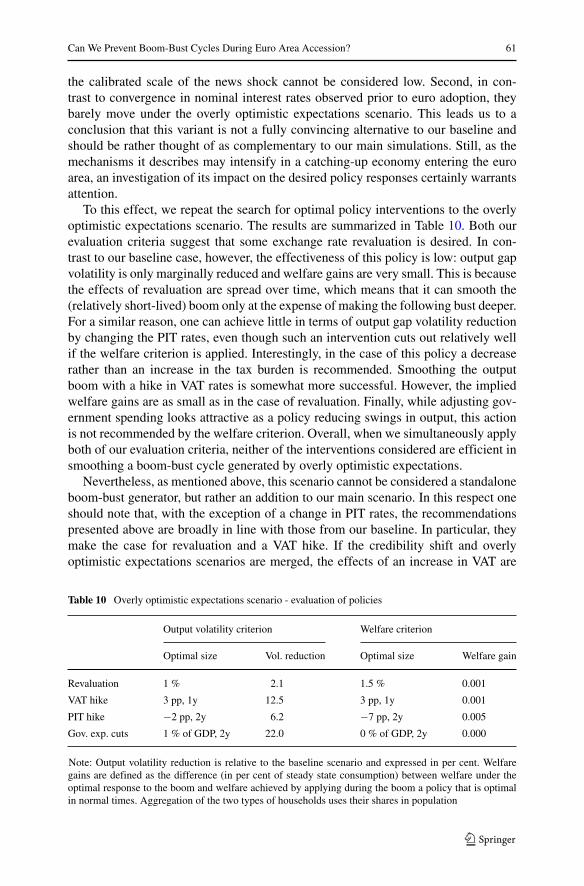
the calibrated scale of the news shock cannot be considered low. Second, in con-trast to convergence in nominal interest rates observed prior to euro adoption, theybarely move under the overly optimistic expectations scenario. This leads us to aconclusion that this variant is not a fully convincing alternative to our baseline andshould be rather thought of as complementary to our main simulations. Still, as themechanisms it describes may intensify in a catching-up economy entering the euroarea, an investigation of its impact on the desired policy responses certainly warrantsattention.

To this effect, we repeat the search for optimal policy interventions to the overlyoptimistic expectations scenario. The results are summarized in Table 10. Both ourevaluation criteria suggest that some exchange rate revaluation is desired. In con-trast to our baseline case, however, the effectiveness of this policy is low: output gapvolatility is only marginally reduced and welfare gains are very small. This is becausethe effects of revaluation are spread over time, which means that it can smooth the(relatively short-lived) boom only at the expense of making the following bust deeper.For a similar reason, one can achieve little in terms of output gap volatility reductionby changing the PIT rates, even though such an intervention cuts out relatively wellif the welfare criterion is applied. Interestingly, in the case of this policy a decreaserather than an increase in the tax burden is recommended. Smoothing the outputboom with a hike in VAT rates is somewhat more successful. However, the impliedwelfare gains are as small as in the case of revaluation. Finally, while adjusting gov-ernment spending looks attractive as a policy reducing swings in output, this actionis not recommended by the welfare criterion. Overall, when we simultaneously applyboth of our evaluation criteria, neither of the interventions considered are efficient insmoothing a boom-bust cycle generated by overly optimistic expectations.

Nevertheless, as mentioned above, this scenario cannot be considered a standaloneboom-bust generator, but rather an addition to our main scenario. In this respect oneshould note that, with the exception of a change in PIT rates, the recommendationspresented above are broadly in line with those from our baseline. In particular, theymake the case for revaluation and a VAT hike. If the credibility shift and overlyoptimistic expectations scenarios are merged, the effects of an increase in VAT are

Table 10 Overly optimistic expectations scenario - evaluation of policies

Output volatility criterion Welfare criterion

Optimal size Vol. reduction Optimal size Welfare gain

Revaluation 1 % 2.1 1.5 % 0.001

VAT hike 3 pp, 1y 12.5 3 pp, 1y 0.001

PIT hike −2 pp, 2y 6.2 −7 pp, 2y 0.005

Gov. exp. cuts 1 % of GDP, 2y 22.0 0 % of GDP, 2y 0.000

Note: Output volatility reduction is relative to the baseline scenario and expressed in per cent. Welfaregains are defined as the difference (in per cent of steady state consumption) between welfare under theoptimal response to the boom and welfare achieved by applying during the boom a policy that is optimalin normal times. Aggregation of the two types of households uses their shares in population


0 20 40 60 80 100−1

0

1

2

3

4

5Output

0 20 40 60 80 100−2

0

2

4

6

8

10Consumption

0 20 40 60 80 100−10

−5

0

5

10

15

20

25Investment

0 20 40 60 80 100−6

−5

−4

−3

−2

−1

0


0 20 40 60 80 100−6

−4

−2

0

2


0 20 40 60 80 100−4

−2

0

2

4

6Inflation

Fig. 12 Easier access to foreign credit scenario. The current account balance is expressed relative tonominal output. Inflation is annualised. All variables are reported as per cent or percentage point deviationsfrom their initial steady state values

somewhat closer to those of revaluation, but the latter still ranks first according toboth optimality criteria. Needless to say, while the implied joint size of revaluation(7.5–8.5 %) still looks acceptable from a political perspective, increasing the VATrates by another 3 pp. over what is implied by our baseline is even more difficultto imagine. All in all, the presented robustness check does not change our mainconclusion of the attractiveness of revaluation.

7.2 Easier Access to Foreign Credit

In order to analyse the impact of foreign credit easing, we make some modificationsto the baseline model. In particular, we assume that Polish households are subjectto a constraint on foreign credit volume, expressed as a percentage of their fixedcapital holdings.14 After joining the euro area, this constraint is gradually loosened(i.e. the loan-to-value ratio increased) so that after five years borrowing from abroadultimately increases by an equivalent of 15 % of Polish GDP. While this number issomewhat arbitrary, we justify it by referring to the experience of relatively poor EUcountries presented in the Introduction. In their case, the net foreign assets positiondeteriorated by an average of 30 % of GDP during the five years following the euroadoption. However, given the recent balance of payments tensions in some euro areacountries, it is reasonable to expect that in the future banks will be less likely totolerate as large increases in foreign debt and hence we assume only half of theincrease in our simulations.

The dynamic responses to this scenario are plotted in Fig. 12. In contrast to theoverly optimistic expectations scenario, this one generates a fully-fledged boom-bust,

14See Appendix for technical details.


Table 11 Easier access to foreign credit scenario - evaluation of policies



Revaluation 6.5 % 32.6 2 % 0.105

VAT hike 16 pp, 1y 19.7 3 pp, 1y 0.003

PIT hike 10 pp, 1y 6.9 1.4 pp, 1y 0.009

Gov. exp. cuts 4.2 % of GDP, 2y 51.2 0 % of GDP, 1y 0.000


similar in nature to our baseline case. Higher borrowing ability fuels consumptionand investment, which leads to a sharp increase in imports and output. However, asprices rise and the real exchange rate appreciates, exports become uncompetitive anddecrease gradually. This brings an end to the boom: output contracts and bottoms outin the fourth year after accession.

As before, we next implement our stabilisation policies. The results are collectedin Table 11. Regarding the output volatility criterion, the most effective policy is thefiscal tightening, followed by the exchange rate revaluation. However, while the lat-ter is also a good policy in terms of welfare improvement, the former is useless forthe reasons described previously. As it was found in the baseline scenario, tax poli-cies seem largely ineffective and require rate adjustments that are not implementablein practice. All in all, if the boom-bust scenario is driven not only by interest rate con-vergence (our baseline), but also by easier access to foreign credit, the main policyconclusions do not change: the exchange rate revaluation seems to be the preferredoption.

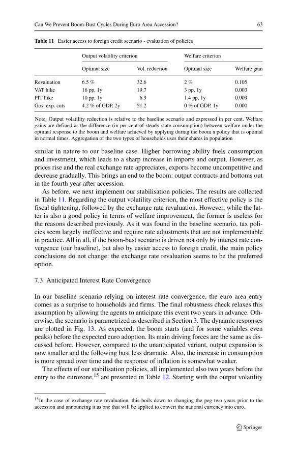
7.3 Anticipated Interest Rate Convergence

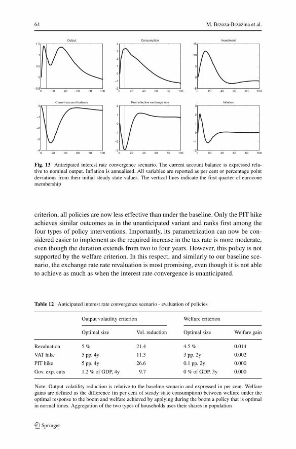
In our baseline scenario relying on interest rate convergence, the euro area entrycomes as a surprise to households and firms. The final robustness check relaxes thisassumption by allowing the agents to anticipate this event two years in advance. Oth-erwise, the scenario is parametrized as described in Section 3. The dynamic responsesare plotted in Fig. 13. As expected, the boom starts (and for some variables evenpeaks) before the expected euro adoption. Its main driving forces are the same as dis-cussed before. However, compared to the unanticipated variant, output expansion isnow smaller and the following bust less dramatic. Also, the increase in consumptionis more spread over time and the response of inflation is somewhat weaker.

The effects of our stabilisation policies, all implemented also two years before theentry to the eurozone,15 are presented in Table 12. Starting with the output volatility

15In the case of exchange rate revaluation, this boils down to changing the peg two years prior to theaccession and announcing it as one that will be applied to convert the national currency into euro.


0 20 40 60 80 100−0.5

0

0.5

1

1.5Output

0 20 40 60 80 100−2

−1

0

1

2

3

4Consumption

0 20 40 60 80 100−5

0

5

10

15Investment

0 20 40 60 80 100−4

−3

−2

−1


0 20 40 60 80 100−3

−2

−1

0

1


0 20 40 60 80 100−2

−1

0

1

2

3Inflation

Fig. 13 Anticipated interest rate convergence scenario. The current account balance is expressed rela-tive to nominal output. Inflation is annualised. All variables are reported as per cent or percentage pointdeviations from their initial steady state values. The vertical lines indicate the first quarter of eurozonemembership

criterion, all policies are now less effective than under the baseline. Only the PIT hikeachieves similar outcomes as in the unanticipated variant and ranks first among thefour types of policy interventions. Importantly, its parametrization can now be con-sidered easier to implement as the required increase in the tax rate is more moderate,even though the duration extends from two to four years. However, this policy is notsupported by the welfare criterion. In this respect, and similarly to our baseline sce-nario, the exchange rate rate revaluation is most promising, even though it is not ableto achieve as much as when the interest rate convergence is unanticipated.

Table 12 Anticipated interest rate convergence scenario - evaluation of policies



Revaluation 5 % 21.4 4.5 % 0.014

VAT hike 5 pp, 4y 11.3 3 pp, 2y 0.002

PIT hike 5 pp, 4y 26.6 0.1 pp, 2y 0.000

Gov. exp. cuts 1.2 % of GDP, 4y 9.7 0 % of GDP, 3y 0.000



8 Conclusions

In this paper we investigate whether boom-bust episodes that have plagued severalcatching-up economies during their euro-area accession (or pegging to the euro) canbe avoided by an appropriate use of macroeconomic policy tools. The boom-bustcycles are a result of sharply declining interest rates in the period shortly preced-ing the euro area accession. Lower interest rates boost domestic demand, output andimports. Over time this brings about higher inflation and deterioration in competi-tiveness. As a result, domestic demand as well as exports decline and the boom turnsinto a bust.

To analyse the ability of monetary and fiscal authorities to smooth the boom, weuse EAGLE, a four-country model developed by Gomes et al. (2012). The modelis changed in three areas in order to fit our needs. First, we calibrate the model toinclude Poland - one of the potential victims of the boom-bust scenario. The secondadjustment is related to a specific feature of the Polish economy - a relatively highimport content of its exports. Since in the original version of EAGLE exports areproduced only domestically, we reconstruct the model so that it now reflects a foreigninput into the production of export goods. Third, in order to perform meaningfulwelfare comparisons across alternative fiscal policies, we incorporate public goodsinto households’ utility function.

Having done this, we first generate the boom-bust scenario. Convergence of inter-est rates generates a temporary boom that resembles the episodes described above.Next, we analyse the impact of four policies (exchange rate revaluation, PIT increase,VAT increase and fiscal contraction) designed to cool down the boom.

We find that all considered policies are able to substantially smooth the boom inoutput. However, they have differentiated effects on other macro variables, some ofthem being undesired. For example, fiscal contraction fuels the consumption boom,and a higher PIT rate increases inflation. From this point of view, the exchange raterevaluation cuts off relatively well, cooling down the output and inflation booms andsubstantially limiting booms in consumption and investment. Of course, this comesat a cost of somewhat increased volatility of exports.

Revaluation is also the preferred policy according to the welfare criterion. Impor-tantly, its optimal magnitude roughly coincides with that minimizing volatility of theoutput gap. This is in contrast to the other policies, for which the welfare analysissuggests a significantly lower size of intervention than that implied by the output gapcriterion, or even no action at all.

Looking at the instrument adjustment minimizing output gap volatility, we findthat the revaluation should amount to ca. 7 %, the VAT rate should be raised by 9 per-centage points, the PIT rate by 12 percentage points and the fiscal contraction shouldamount to around 2 % of GDP. Thus, from the political perspective, the analysed taxpolicies seem impossible to implement. On the other hand, both the exchange raterevaluation and fiscal contraction seem to be of reasonable magnitudes. Taking allthese considerations together, we conclude that revaluation is the most promising toolin smoothing out the boom-bust cycle. This conclusion still holds when we allow forthe fact that the boom-bust episodes observed in catching-up economies during their


euro accession may additionally reflect a build-up of overly optimistic expectationsabout the real convergence processes or result from easier access to foreign credit.

One should keep in mind that all policies considered in this paper have beendesigned to trim a boom-bust cycle in domestic demand. They should not be expectedto prevent asset price bubbles, if these are going to emerge after euro area acces-sion. This important and interesting problem qualifies for another study using anothermodel.

Acknowledgments The paper was written while Michał Brzoza-Brzezina was visiting the EuropeanCentral Bank. We would like to thank Grzegorz Dobroczek, Ewa Korzyc, Wojciech Mroczek, Gabor Pula,Ieva Rubene, Daria Taglioni and Maria Valderrama for their help in obtaining the data. We also greatlyappreciate the comments received from Jan Bruha, Guter Coenen, Giancarlo Corsetti, Juergen von Hagen,Stefan Laseen, Bartosz Mackowiak, Reiner Martin, Dobromił Serwa and an anonymous referee, as wellas participants of the seminars at the European Central Bank, the Narodowy Bank Polski, the WarsawSchool of Economics, the Central Bank Macroeconomic Modeling Workshop, the CEUS Workshop, theICMAIF conference, the IES conference and the meeting of the ESBC Working Group on EconometricModeling. This article should not be reported as representing the views of the the Narodowy Bank Polskior the European Central Bank (ECB).The views expressed are those of the authors and do not necessarilyreflect those of the Narodowy Bank Polski or the ECB.

Appendix: Extending EAGLE for collateral constraints

In EAGLE there are two types of households. Type I households have access tofinancial markets, where they buy and sell domestic government bonds and inter-nationally traded bonds, accumulate physical capital and rent its services to firms,and hold money for transaction purposes. J-type households do not trade in financialand physical assets and hence can smooth their consumption intertemporally only byadjusting their holdings of money.

In this extension we assume that I-type households are subject to financial frictionsin the form of collateral constraints on foreign borrowing (e.g., Kiyotaki and Moore1997; Mendoza 2006). For the sake of brevity, symbols that are unchanged withrespect to the original EAGLE documentation (Gomes et al. 2012) are not describedagain.

More specifically, the lifetime utility function of i-th household of type I:

Et

{ ∞∑k=0

βk

(1 − κ

1 − σ

(CI,t+k(i) − κCI,t+k−1

1 − κ

)1−σ)− 1

1 + ζNt+k(i)

1+ζ

}(1)

is maximised subject to the budget constraint:(1 + τC

t + �v (vt (i)))

PC,tCt (i) + Pi,t It (i) + R−1t Bt+1(i)

+((

1 − �B∗

(S

H,USt B∗

t+1

PY,tYt

; rpt

))R∗

t

)−1

SH,USt B∗

t+1(i)

+ Mt(i) + �t(i) + t =(1 − τN

t − τWht

)Wt(i)Nt (i) +

(1 − τK

t

) (RK,tut (i) − �u (ut (i)) PI,t

)Kt(i)

+τKt δPI,tKt (i)+

(1 − τD

t

)Dt(i)+T Rt (i) − Tt (i) + Bt (i) + S

H,USt B∗

t (i) + Mt−1(i) (2)


the law of motion for the capital stock:

Kt+1(i) = (1 − δ)Kt (i) +(

1 − �I

(It (i)

It−1(i)

))It (i) (3)

and the collateral constraint:

SH,USt B∗

t+1 ≤ mt (1 − δ) Kt+1(i)EtPI,t+1 (4)

where mt is the loan-to-value (LTV) ratio. In the spirit of Iacoviello (2005), weassume that constraint (4) is always binding, which is achieved by assuming that Pol-ish households are relatively impatient (i.e., they discount the future more heavilythan their foreign counterparts).

The first-order condition wrt. Kt+1 can then be written:

−βEt

{�t+1

PC,t+1

[(1 − τK

t+1

) (RK,t+1ut+1(i) − �u (ut+1(i)) PI,t+1

) + τKt+1δPI,t+1

]}

+�tQt − β(1 − δ)Et {�t+1Qt+1} − (1 − δ)μt

PC,t

mtEtPI,t+1 = 0 (5)

where �t/PC,t , Qt�t and μt/PC,t are Lagrange multipliers associated respectivelywith budget constraint (2), capital accumulation rule (3) and collateral constraint (4).

Rearranging terms and using the equilibrium result that PI,t /PC,t = Qt yields:

Qt = βEt

{�t+1

�t

[(1 − τK

t+1

) (RK,t+1

PC,t+1ut+1(i) − �u (ut+1(i))

PI,t+1

PC,t+1

)

+δτKt+1

PI,t+1

PC,t+1+ (1 − δ) Qt+1

]}+ (1 − δ)

μt

�t

mtEt

{Qt+1�C,t+1

}(6)

The first-order condition wrt. foreign bond holdings now becomes:

�t

((1 − �B∗

(S

H,USt B∗

t+1

PY,tYt

; rpt

))R∗

t

)−1

= βEt

{�t+1

�C,t+1

SH,USt+1

SH,USt

}− μt (7)

The rest of the equilibrium conditions remain unchanged. If we assume that the col-lateral constraint never binds, i.e., μt = 0, we obtain the frictionless version ofEAGLE.

References

Adam K, Billi RM (2008) Monetary conservatism and fiscal policy. J Monet Econ 55(8):1376–1388Adolfson M, Laseen S, Linde J, Villani M (2007) Bayesian estimation of an open economy DSGE model

with incomplete pass-through. J Int Econ 72(2):481–511Almeida V, Castro G, Felix R (2009) The Portuguese economy in the European context: structure,

shocks and policy. In: The Portuguese economy in the context of economic, financial and monetaryintegration, (Banco de Portugal)

Angeloni I, Ehrmann M (2007) Euro area inflation differentials. B.E. J Macroecon 7(1):24


Bayoumi T, Laxton D, Faruqee H, Hunt B, Karam PD, Lee J, Rebucci A, Tchakarov I (2004) GEM: a newinternational macroeconomic model. IMF Occasional Papers 239, International Monetary Fund

Blanchard O (2007) Adjustment within the euro: the difficult case of Portugal. Port Econ J 6(1):1–21Blanchard O, Giavazzi F (2002) Current account deficits in the euro area: the end of the Feldstein Horioka

puzzle? Brook Pap Econ Act 33(2002–2):147–210Brixiova Z, Vartia L, Worgotter A (2009) Capital inflows, household debt and the boom-bust cycle in

Estonia. OECD Economics Department Working Papers 700, OECD, Economics DepartmentBrzoza-Brzezina M (2005) Lending booms in the new EU member states - will euro adoption matter?

Working Paper Series 543, European Central BankChristiano LJ, Eichenbaum M, Evans CL (2005) Nominal rigidities and the dynamic effects of a shock to

monetary policy. J Polit Econ 113(1):1–45Christoffel K, Coenen G, Warne A (2008) The new area-wide model of the euro area - a micro-founded

open-economy model for forecasting and policy analysis. Working Paper Series 944, EuropeanCentral Bank

Coenen G, Vetlov I (2009) Extending the NAWM for the import content of exports. Mimeo, EuropeanCentral Bank

Coenen G, Mohr M, Straub R (2008) Fiscal consolidation in the euro area: long-run benefits and short-runcosts. Econ Model 25(5):912–932

Coenen G, McAdam P, Straub R (2008) Tax reform and labour-market performance in the euro area: asimulation-based analysis using the new area-wide model. J Econ Dyn Control 32(8):2543–2583

Daras T, Hagemejer J (2009) The long run-effects of Poland’s accession to the eurozone. Simulation usingPOLDYN - a dynamic computable general equilibrium model. Working Paper Series 70, NationalBank of Poland

ECB (2003) Inflation differentials in the euro area: potential causes and policy implications. Technicalreport. European Central Bank

Eichengreen B, Steiner K (2008) Is Poland at risk of a boom-and-bust cycle in the run-up to euro adoption?NBER Working Papers 14438, National Bureau of Economic Research, Inc.

Erceg CJ, Guerrieri L, Gust C (2006) SIGMA: a new open economy model for policy analysis. Int J CentBank 2(1):1–50

Fagan G, Gaspar V (2007) Adjusting to the euro. Working Paper Series 716, European Central BankFaruqee H, Laxton D, Muir D, Pesenti PA (2007) Smooth landing or crash? Model-based scenarios of

global current account rebalancing. In: G7 current account imbalances: sustainability and adjustment,NBER Chapters, (National Bureau of Economic Research, Inc.), pp 377–456

Gomes S, Jacquinot P, Pisani M (2012) The EAGLE: a model for policy analysis of macroeconomicinterdependence in the euro area. Econ Model 29(5):1686–1714

Grabek G, Klos B, Koloch G (2011) SOEPL 2009 - An estimated dynamic stochastic general equilibriummodel for policy analysis and forecasting. National Bank of Poland Working Papers 83, NationalBank of Poland, Economic Institute

Gradzewicz M, Makarski K (2013) The macroeconomic effects of losing autonomous monetary policyafter the euro adoption in Poland. Appl Econ 45(17):2443–2455

Honohan P, Leddin AJ (2006) Ireland in EMU - more shocks, less insulation? Econ Soc Rev 37(2):263–294

Honohan P, Lane PR (2003) Divergent inflation rates in EMU. Econ Pol 18(37):357–394Iacoviello M (2005) House prices, borrowing constraints, and monetary policy in the business cycle. Am

Econ Rev 95(3):739–764Kiyotaki N, Moore J (1997) Credit cycles. J Polit Econ 105(2):211–48Kolasa M (2009) Structural heterogeneity or asymmetric shocks? Poland and the euro area through the

lens of a two-country DSGE model. Econ Model 26(6):1245–1269Kolasa M (2014) Real convergence and its illusions. Econ Model 37(C):79–88Kuodis R, Ramanauskas T (2009) From boom to bust: lessons from Lithuania. Monetary Studies 1,

Lietuvos BankasLopez-Salido D, Restoy F, Valles J (2005) Inflation differentials in EMU: the Spanish case. Banco de

Espana Working Papers 0514, Banco de EspanaLucas RE (2003) Macroeconomic priorities. Am Econ Rev 93(1):1–14Mendoza EG (2006) Endogenous sudden stops in a business cycle model with collateral constraints: a fish-

erian deflation of Tobin’s Q. NBER Working Papers 12564, National Bureau of Economic Research,Inc., October


Schadler S, Drummond N, Flavio P, Kuijs L, Murgasova Z, van Elkan R (2005) Adopting the euro inCentral Europe: challenges of the next step in European integration. IMF Occasional Papers 234,International Monetary Fund

Siedschlag I, von Hagen J (2006) Macroeconomic adjustment in the new EU member states, Vol 42-1 ofChapters in SUERF Studies

Smets F, Wouters R (2003) An estimated dynamic stochastic general equilibrium model of the euro area.J Eur Econ Assoc 1(5):1123–1175

Zdarek V, Aldasoro JI (2009) Inflation differentials in the euro area and their determinants - an empiricalview. Kiel Advanced Studies Working Papers 450, Kiel Institute for the World Economy

Date post:	23-Dec-2016
Category:	Documents
Upload:	marcin
View:	217 times
Download:	2 times

Can We Prevent Boom-Bust Cycles During Euro Area Accession?

Documents