87
Capacity Building Workshop Python for Climate Data Analysis Christoph Menz November 26, 2019

Capacity Building WorkshopPython for Climate Data Analysis
Christoph Menz
November 26, 2019
Module Overview
• Lecture: Introduction to Python• Hands-On: Python for Beginners• Exercise: Python• Lecture: Introduction to Python Libraries• Hands-On: Access and analysis of netCDF Data with Python• Lecture: Python Libraries for Data Visualization• Hands-On: Visualization of Scientific Data with matplotlib• Hands-On: Visualization of Geospatial Data with cartopy• Exercise: Analysis and Visualization of netCDF Data with
python
,Christoph Menz RD II: Climate Resilience 2

Introduction to Python
,Christoph Menz RD II: Climate Resilience 3
Introduction to Python
• High-level general-purpose programming language• Emerges in the late 80s and early 90s (first release 1991)• Based on teaching/prototyping language ABC• Freely available under Python Software Foundation License• Major design philosophy: readability and performance• Important features:
• Dynamic types (type automatically declared and checked atruntime)
• Automatized memory management• Objects, Loops, Functions• Easily extendible by various libraries (numpy, netCDF4,
scikit-learn, ...)
,Christoph Menz RD II: Climate Resilience 4
Scope of this Course
• Basic programming and scripting with python• Read, preparation, statistics and visualization of netCDF
based data• Focus on python version 3.x using Anaconda platform• Online Tutorials:
Anaconda Tutorialshttps://docs.python.org/3/tutorialhttps://www.tutorialspoint.com/python3https://scipy.org & http://scikit-learn.orghttps://matplotlib.org/http://scitools.org.uk/cartopy
,Christoph Menz RD II: Climate Resilience 5

Anaconda - Data Science Platform
,Christoph Menz RD II: Climate Resilience 6

Jupyter - Interactive Computing Notebook
,Christoph Menz RD II: Climate Resilience 7
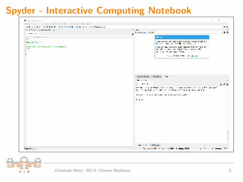
Spyder - Interactive Computing Notebook
,Christoph Menz RD II: Climate Resilience 8

Variables in python
• Variable types are automatically defined at runtime
variable_name = value
• Uses dynamic and static type casting:• 5*5.0 is a float and "Hello world" is a string• str(5) is a string and int("9") is a integer
• python got 13 different built-in types:• bool, int, float, str, list, tuple, dict, bytearray, bytes,
complex, ellipsis, frozenset, set• Possibility to create your own type for object-oriented
programming ( class statement)
,Christoph Menz RD II: Climate Resilience 9
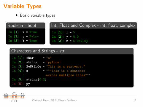
Variable Types• Basic variable types
Boolean - boolIn [1]: x = TrueIn [2]: y = FalseIn [3]: Y = True
Int, Float and Complex - int, float, complexIn [1]: x = 5In [2]: y = 5.0In [3]: z = 5.0+2.0j
Characters and Strings - strIn [1]: char = "a"In [2]: string = 'python'In [3]: SeNtEnCe = "This is a sentence."In [4]: x = """This is a sentence
...: across multiple lines"""In [5]: string[0:2]In [5]: py
,Christoph Menz RD II: Climate Resilience 10
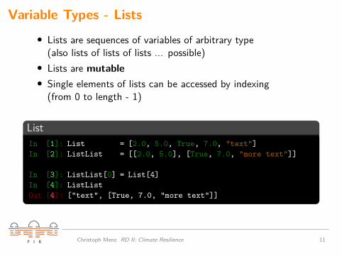
Variable Types - Lists• Lists are sequences of variables of arbitrary type
(also lists of lists of lists ... possible)• Lists are mutable• Single elements of lists can be accessed by indexing
(from 0 to length - 1)
ListIn [1]: List = [2.0, 5.0, True, 7.0, "text"]In [2]: ListList = [[2.0, 5.0], [True, 7.0, "more text"]]
In [3]: ListList[0] = List[4]In [4]: ListListOut [4]: ["text", [True, 7.0, "more text"]]
,Christoph Menz RD II: Climate Resilience 11

Variable Types - Tuples• Tuples are similar to lists• But tuples are immutable
TupleIn [1]: Tuple = (2.0, 5.0, True, 7.0, "text")In [2]: TupleTuple = ((2.0, 5.0), (True, 7.0, "more text"))
In [3]: TupleTuple[0] = Tuple[4]----------------------------------------------------------------TypeError Traceback (most recent call last)<ipython-input-52-862d5dc2e8bb> in <module> ()----> 1 TupleTuple [0] = Tuple [4]
TypeError : 'tuple' object does not support item assignment
,Christoph Menz RD II: Climate Resilience 12

Variable Types - Dictionaries• Dictionaries are unordered collections of arbitrary variables• Dictionaries are mutable• Elements of dictionaries get accessed by keys instead of
indices• Keys in dictionaries are unique
DictionaryIn [1]: my_dict = {"a":2.0, "b":5.0, "zee":[True, True]}In [2]: my_dict["b"] = 23.0In [3]: my_dictOut [3]: {'a':2.0, 'b':23, 'zee':[True,True]}In [4]: {"a":2.0, "b":5.0, "zee":[True, True], "a":7}Out [4]: {'a':7, 'b':5.0, 'zee':[True,True]}
,Christoph Menz RD II: Climate Resilience 13

Operations
Addition & SubtractionIn [1]: 3 + 5.0Out [1]: 8.0In [2]: 3 - 5Out [2]: -2
Multiplication & DivisionIn [1]: 4 * 4Out [1]: 16In [2]: 8 / 2Out [2]: 4.0In [3]: 7 // 3Out [3]: 2In [4]: 7 % 3Out [4]: 1
• python supports the usualmathematical operations onfloat, int and complex
• Dynamic casting depends onoperator and variable type
Power & RootIn [1]: 4**2Out [1]: 16In [2]: 4**2.5Out [2]: 32.0In [3]: 16**0.5Out [3]: 4.0
,Christoph Menz RD II: Climate Resilience 14
Boolean Operations
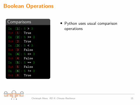
ComparisonsIn [1]: 5 > 3Out [1]: TrueIn [2]: 5 >= 3Out [2]: TrueIn [3]: 5 < 3Out [3]: FalseIn [4]: 5 <= 3Out [4]: FalseIn [5]: 5 == 3Out [5]: FalseIn [6]: 5 != 3Out [6]: True
• Python uses usual comparisonoperations
• in -Operator permits an easy searchfunctionality
in-OperatorIn [7]: 7 in [1, 2, 3, 4, 5]Out [7]: FalseIn [8]: "b" in {"a":4, "b":6, "c":8}Out [8]: True
,Christoph Menz RD II: Climate Resilience 15

Boolean Operations
ComparisonsIn [1]: 5 > 3Out [1]: TrueIn [2]: 5 >= 3Out [2]: TrueIn [3]: 5 < 3Out [3]: FalseIn [4]: 5 <= 3Out [4]: FalseIn [5]: 5 == 3Out [5]: FalseIn [6]: 5 != 3Out [6]: True
• Python uses usual comparisonoperations
• in -Operator permits an easy searchfunctionality
in-OperatorIn [7]: 7 in [1, 2, 3, 4, 5]Out [7]: FalseIn [8]: "b" in {"a":4, "b":6, "c":8}Out [8]: True
,Christoph Menz RD II: Climate Resilience 15

Boolean Operators
• python supports the basic logicaloperators to combine booleans
Logical NOTOperator Results
not True Falsenot False True
Logical ANDx Operator y Results
True and True TrueTrue and False False
False and True FalseFalse and False False
Logical ORx Operator y Results
True or True TrueTrue or False TrueFalse or True TrueFalse or False False
,Christoph Menz RD II: Climate Resilience 16

Methods of Objects/Variables
• Python variables are notjust atomic variables
• Python variables areobjects by themself
• Each variable alreadycomes with associatedmethods
• Syntax:variable.method
Object methodsIn [1]: x = []In [2]: x.append(3)In [3]: x.append(5)In [4]: print(x)[3,5]In [5]: y = {"a":1,"b":2,"c":3}In [6]: print(y.keys())dict_keys(['a','b','c'])In [7]: "This is a sentence".split(" ")In [7]: ['This','is','a','sentence']In [8]: " ".join(["This","is","a","list"])In [8]: 'This is a list'
You can use the dir() function to get an overview of all methodsavailable for a given variable.
,Christoph Menz RD II: Climate Resilience 17

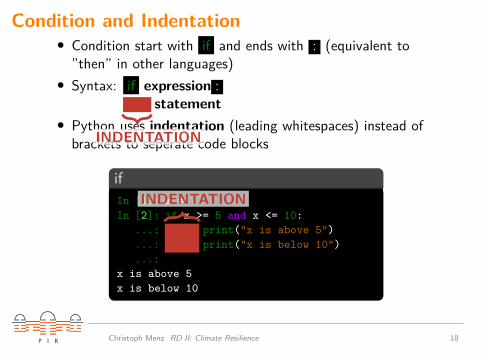
Condition and Indentation• Condition start with if and ends with : (equivalent to
”then” in other languages)• Syntax: if expression :
statement
• Python uses indentation (leading whitespaces) instead ofbrackets to seperate code blocks
ifIn [1]: x = 7In [2]: if x >= 5 and x <= 10:
...: print("x is above 5")
...: print("x is below 10")
...:x is above 5x is below 10
INDENTATION
INDENTATION
,Christoph Menz RD II: Climate Resilience 18

Condition and Indentation• Condition start with if and ends with : (equivalent to
”then” in other languages)• Syntax: if expression :
statement• Python uses indentation (leading whitespaces) instead of
brackets to seperate code blocks
ifIn [1]: x = 7In [2]: if x >= 5 and x <= 10:
...: print("x is above 5")
...: print("x is below 10")
...:x is above 5x is below 10
INDENTATION
INDENTATION
,Christoph Menz RD II: Climate Resilience 18
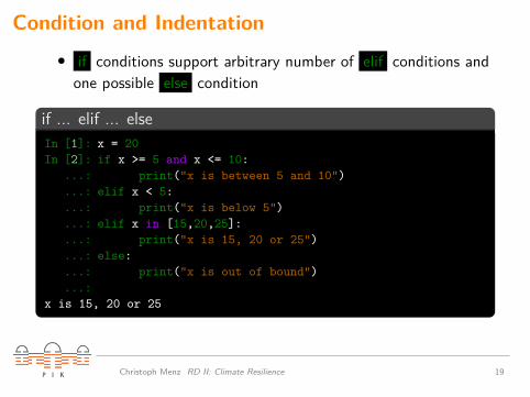
Condition and Indentation• if conditions support arbitrary number of elif conditions and
one possible else condition
if ... elif ... elseIn [1]: x = 20In [2]: if x >= 5 and x <= 10:
...: print("x is between 5 and 10")
...: elif x < 5:
...: print("x is below 5")
...: elif x in [15,20,25]:
...: print("x is 15, 20 or 25")
...: else:
...: print("x is out of bound")
...:x is 15, 20 or 25
,Christoph Menz RD II: Climate Resilience 19

Loops• For loops iterate only a specific number of times• Syntax: for variable in iterable :
statement• Iterable are objects you can iterate over (list, tuple, dict,
iterators, etc.)
for-LoopIn [1]: for x in [2,4,6,8]:
...: print(x*2)
...:481216
,Christoph Menz RD II: Climate Resilience 20
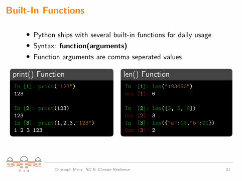
Built-In Functions
• Python ships with several built-in functions for daily usage• Syntax: function(arguments)• Function arguments are comma seperated values
print() FunctionIn [1]: print("123")123
In [2]: print(123)123In [3]: print(1,2,3,"123")1 2 3 123
len() FunctionIn [1]: len("123456")Out [1]: 6
In [2]: len([3, 5, 8])Out [2]: 3In [3]: len({"a":13,"b":21})Out [3]: 2
,Christoph Menz RD II: Climate Resilience 21

Type Related Built-In Functions
• Use the type() function toget the type of any variable
• Type conversion can bedone using one of thefollowing functions:bool(), int(), float(), str(),list(), tuple(), dict()
type() FunctionIn [1]: type("PyThOn")Out [1]: strIn [2]: type(3)Out [2]: intIn [3]: type(3.0)Out [3]: floatIn [4]: type({"a":13,"b":21})Out [4]: dict
Type Conversion IIn [1]: bool(0)Out [1]: FalseIn [2]: bool(2.2)Out [2]: TrueIn [3]: int(2.8)Out [3]: 2
Type Conversion IIIn [1]: list((2,3,5))Out [1]: [2, 3, 5]In [2]: tuble([2,3,5])Out [2]: (2, 3, 5)In [3]: float("3.14")Out [3]: 3.14
,Christoph Menz RD II: Climate Resilience 22

Mathematical Built-In Functions• Python supports basic mathematical operations• Work on numbers: abs and round• Work on list and tuples: min, max, sum and sorted
abs() and round()In [1]: abs(-5)Out [1]: 5In [2]: round(24.03198)Out [2]: 24In [3]: round(24.03198,3)Out [3]: 24.032
min(), max(), sum() and sorted()In [1]: min([55,89,144,233])Out [1]: 55In [2]: max([55,89,144,233])Out [2]: 233In [3]: sum([55,89,144,233])Out [3]: 521In [4]: sorted([12,3,17,3])Out [4]: [3, 3, 12, 17]In [5]: sorted(["b","aca","aaa","cd"])Out [5]: ['aaa', 'aca', 'b', 'cd']
,Christoph Menz RD II: Climate Resilience 23

Help Built-In Function• The most important built-in function is help()• Gives you a short description on the given argument
(variables or other functions)
help()In [1]: help(max)Help on built-in function max in module builtins:
max(...)max(iterable, *[, default=obj, key=func]) -> valuemax(arg1, arg2, *args, *[, key=func]) -> value
With a single iterable argument, return its biggest item. Thedefault keyword-only argument specifies an object to return ifthe provided iterable is empty.With two or more arguments, return the largest argument.
,Christoph Menz RD II: Climate Resilience 24
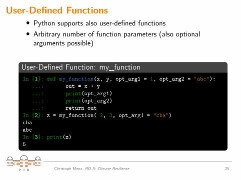
User-Defined Functions• Python supports also user-defined functions• Arbitrary number of function parameters (also optional
arguments possible)
User-Defined Function: my_functionIn [1]: def my_function(x, y, opt_arg1 = 1, opt_arg2 = "abc"):
...: out = x + y
...: print(opt_arg1)
...: print(opt_arg2)
...: return outIn [2]: z = my_function( 2, 3, opt_arg1 = "cba")cbaabcIn [3]: print(z)5
mandatoryparameters
optionalparameters
,Christoph Menz RD II: Climate Resilience 25
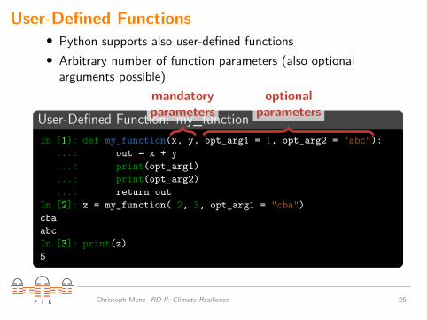

Hands-On: Python forBeginners
,Christoph Menz RD II: Climate Resilience 26
Exercise: Python
,Christoph Menz RD II: Climate Resilience 27

Exercise
1. Test if the following operations between various types arepossible: float*int, bool*int, bool*float, bool+bool,string*bool, string*int, string*float, string+int
2. What is the result of the following operations:["a","b","c"]*3, (1,2,3)*3 and{"a":1,"b":2,"c":3}*3. Could you explain why the lastoperation isn’t working?
3. Print all even numbers between 0 and 100 to the screen (hint:use a for loop and if condition).
,Christoph Menz RD II: Climate Resilience 28

Exercise4. Write a function that calculates the mean of a given list of
floats (hint: use sum() and len()).5. Write a function that calculates the median of a given list of
floats (hint: use sorted() and len() to determine thecentral value of the sorted list, use if condition to distinguishbetween even and odd length lists).
6. Test your mean and median function with the following lists:
list mean median[4,7,3,2,7,4,2] 4.143 4.0[2,6,3,1,8,5,4] 4.143 4.0[2,1,4,5,7,9] 4.667 4.5[2,7,4,8,5,1] 4.500 4.5
,Christoph Menz RD II: Climate Resilience 29

Introduction to PythonLibraries
,Christoph Menz RD II: Climate Resilience 30

Libraries• Basic functionality of python is limited• Libraries extend the functionality of python to various fields
(I/O of various formats, math/statistics, visualization, etc.)• Import syntax: import <library>• Sublibrary/Function import:
from <library> import <sublibrary/function>• Use syntax: <library>.<sublibrary/function>
LibrariesIn [1]: import osIn [2]: from os import listdirIn [3]: listdir("/")In [3]: ['root','etc','usr','bin', ... ,'srv','tmp','mnt']In [4]: import numpy as npIn [4]: np.sqrt(2)In [3]: 1.4142135623730951
,Christoph Menz RD II: Climate Resilience 31

Python Package Index
• Search for libraries on the web• Short description, install instructions and source files
https://pypi.org
,Christoph Menz RD II: Climate Resilience 32

Install with Anaconda Navigator• Anaconda Navigator can install libraries (→ Environment)• You can install multiple environments with different libraries
,Christoph Menz RD II: Climate Resilience 33

Important Libraries
os OS routines implementation in pythoncftime Implementation of date and time objects
numpy Fast general-purpose processing of multi-dimensionalarrays
scikit-learn Machine-learning routines in python
pandas Easy and intuitive handling of structured and timeseries data
netCDF4 I/O of netCDF filesmatplotlib Basic 2D visualization in python
cartopy Draw geospatial data in python
,Christoph Menz RD II: Climate Resilience 34

Introduction topython-numpy
,Christoph Menz RD II: Climate Resilience 35

Introduction to python-numpyFast general-purpose processing for large multidimensional arrays
• Implements a powerful N-dimensional array type(huge improvement over lists/tuples)
• Basic linear algebra, Fourier transform, and random numbercapabilities
• I/O of formated and unformated data• Based on C and FORTRAN77 routines in the background• Requirement for most scientific python libraries (matplotlib,
pandas, netCDF4, etc.)
Import NumpyIn [1]: import numpy as np
,Christoph Menz RD II: Climate Resilience 36
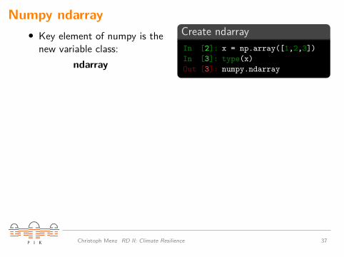
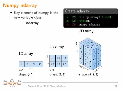
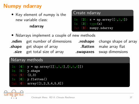
Numpy ndarray• Key element of numpy is the
new variable class:ndarray
Create ndarrayIn [2]: x = np.array([1,2,3])In [3]: type(x)Out [3]: numpy.ndarray
• Ndarrays implement a couple of new methods.ndim get number of dimensions
.shape get shape of array.size get total size of array
.reshape change shape of array.flatten make array flat
.swapaxes swap dimensions
Ndarray methodsIn [4]: y = np.array([[1,2,3],[4,5,6]])In [5]: y.shapeOut [5]: (2,3)In [6]: y.flatten()Out [6]: array([1,2,3,4,5,6])
,Christoph Menz RD II: Climate Resilience 37
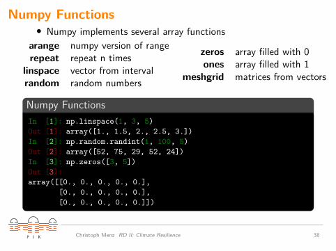
Numpy Functions• Numpy implements several array functions
arange numpy version of rangerepeat repeat n times
linspace vector from intervalrandom random numbers
zeros array filled with 0ones array filled with 1
meshgrid matrices from vectors
Numpy FunctionsIn [1]: np.linspace(1, 3, 5)Out [1]: array([1., 1.5, 2., 2.5, 3.])In [2]: np.random.randint(1, 100, 5)Out [2]: array([52, 75, 29, 52, 24])In [3]: np.zeros([3, 5])Out [3]:array([[0., 0., 0., 0., 0.],
[0., 0., 0., 0., 0.],[0., 0., 0., 0., 0.]])
,Christoph Menz RD II: Climate Resilience 38

Math Functions• Mathematical functions for elementwise evaluation
ExponentialIn [1]: np.exp([0, 1, np.log(2)])Out [1]: array([1. , 2.71828183, 2. ])In [2]: np.log([0, np.e, np.e**0.5])Out [2]: array([0. , 1. , 0.5])
exp and log are defined asnatural exponential andlogarithm (base e)
log is invers to exp
Trigonometric FunctionsIn [1]: x = np.array([0, np.pi, 0.5*np.pi])In [2]: np.sin(x)Out [2]: array([0., 0., 1.])In [3]: np.cos(x)Out [3]: array([1., -1., 0.])In [4]: np.tan(x)Out [4]: array([0., 0., 0.])
Further Functionsarcsin, arccos, arctan,deg2rad, rad2deg, sinh,cosh, tanh, arcsinh,arccosh, arctanh, sqrt,log2, log10, exp2, ...
,Christoph Menz RD II: Climate Resilience 39

Statistical Functions
• Numpy implements usualstatistical functions
• Implementation as function(np.mean) and arraymethod (x.mean)
mean: mean(x, axis = <axis>)sum: sum(x, axis = <axis>)
median: median(x, axis = <axis>)maximum: max(x, axis = <axis>)minimum: min(x, axis = <axis>)
<axis>: dimensions along to evaluate(int or tuple of ints)
Statistic Functions IIn [1]: x = np.random.random((4,2,8))In [2]: np.mean(x)Out [2]: 0.46376In [3]: x.sum(axis = (0,2))Out [3]: array([15.59966 , 14.08082])In [4]: np.median(x)Out [4]: 0.38988
Statistic Functions IIIn [5]: np.min(x, axis = 2)Out [5]: array([[0.0381, 0.2301],
[0.0220, 0.1045],[0.1903, 0.2746],[0.0539, 0.0203]])
In [6]: x.max()Out [6]: 0.9788
,Christoph Menz RD II: Climate Resilience 40

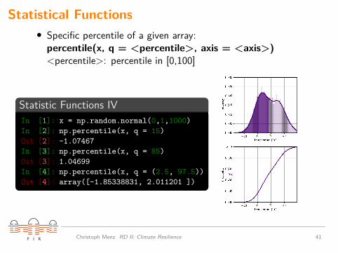
Statistical Functions• Specific percentile of a given array:
percentile(x, q = <percentile>, axis = <axis>)<percentile>: percentile in [0,100]
Statistic Functions IVIn [1]: x = np.random.normal(0,1,1000)In [2]: np.percentile(x, q = 15)Out [2]: -1.07467In [3]: np.percentile(x, q = 85)Out [3]: 1.04699In [4]: np.percentile(x, q = (2.5, 97.5))Out [4]: array([-1.85338831, 2.011201 ])
,Christoph Menz RD II: Climate Resilience 41
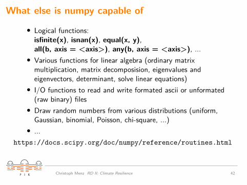
What else is numpy capable of
• Logical functions:isfinite(x), isnan(x), equal(x, y),all(b, axis = <axis>), any(b, axis = <axis>), ...
• Various functions for linear algebra (ordinary matrixmultiplication, matrix decomposision, eigenvalues andeigenvectors, determinant, solve linear equations)
• I/O functions to read and write formated ascii or unformated(raw binary) files
• Draw random numbers from various distributions (uniform,Gaussian, binomial, Poisson, chi-square, ...)
• ...https://docs.scipy.org/doc/numpy/reference/routines.html
,Christoph Menz RD II: Climate Resilience 42
Introduction topython-netCDF4
,Christoph Menz RD II: Climate Resilience 43

Introduction to python-netCDF4
• Read and write netCDF4 files in python• Based on Unidata group netCDF4-C libraries• Uses python-numpy arrays to store data in python• We will cover only the read-functionality in this course
python-netCDF4In [1]: from netCDF4 import DatasetIn [2]: from cftime import num2date
Dataset Main object to read and write netCDF filesnum2date Contains functions to translate the dates
,Christoph Menz RD II: Climate Resilience 44
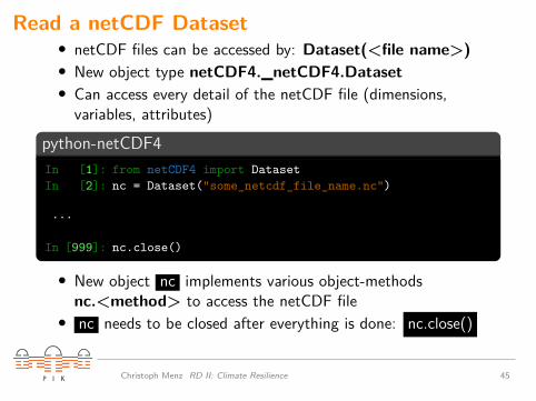
Read a netCDF Dataset• netCDF files can be accessed by: Dataset(<file name>)• New object type netCDF4._netCDF4.Dataset• Can access every detail of the netCDF file (dimensions,
variables, attributes)
python-netCDF4In [1]: from netCDF4 import DatasetIn [2]: nc = Dataset("some_netcdf_file_name.nc")
...
In [999]: nc.close()
• New object nc implements various object-methodsnc.<method> to access the netCDF file
• nc needs to be closed after everything is done: nc.close()
,Christoph Menz RD II: Climate Resilience 45

Access Global Attributes• Get list of all global attributes: nc.ncattrs()• Get value of specific attribute: nc.getncattr(”<attribute>”)
Access Global AttributesIn [3]: nc.ncattrs()In [3]:['institution','institute_id','experiment_id',...'cmor_version']In [4]: nc.getncattr("institution")In [4]: 'Max Planck Institute for Meteorology'In [5]: nc.getncattr("experiment")In [5]: 'RCP8.5'
,Christoph Menz RD II: Climate Resilience 46

Access Dimensions• Get a dictionary of all dimension: nc.dimensions
(not a function)
Access DimensionsIn [3]: nc.dimensions.keys()In [3]: odict_keys(['time', 'lat', 'lon', 'bnds'])In [4]: nc.dimensions["time"].nameIn [4]: 'time'In [5]: nc.dimensions["time"].sizeIn [5]: 1461In [6]: nc.dimensions["time"].isunlimitedIn [6]: True
nc.dimensions[”<dim>”].name name of <dim>nc.dimensions[”<dim>”].size size of <dim>
nc.dimensions[”<dim>”].isunlimited() True if <dim> is record(size of record dimensions (time) can increase unlimited)
,Christoph Menz RD II: Climate Resilience 47
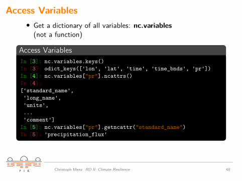
Access Variables• Get a dictionary of all variables: nc.variables
(not a function)
Access VariablesIn [3]: nc.variables.keys()In [3]: odict_keys(['lon', 'lat', 'time', 'time_bnds', 'pr'])In [4]: nc.variables["pr"].ncattrs()In [4]:['standard_name','long_name','units',...'comment']In [5]: nc.variables["pr"].getncattr("standard_name")In [5]: 'precipitation_flux'
,Christoph Menz RD II: Climate Resilience 48
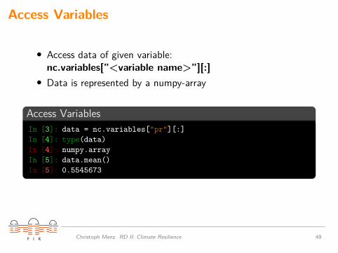
Access Variables
• Access data of given variable:nc.variables[”<variable name>”][:]
• Data is represented by a numpy-array
Access VariablesIn [3]: data = nc.variables["pr"][:]In [4]: type(data)In [4]: numpy.arrayIn [5]: data.mean()In [5]: 0.5545673
,Christoph Menz RD II: Climate Resilience 49
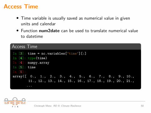
Access Time
• Time variable is usually saved as numerical value in givenunits and calendar
• Function num2date can be used to translate numerical valueto datetime
Access TimeIn [3]: time = nc.variables["time"][:]In [4]: type(time)In [4]: numpy.arrayIn [5]: timeIn [5]:array([ 0., 1., 2., 3., 4., 5., 6., 7., 8., 9., 10.,
11., 12., 13., 14., 15., 16., 17., 18., 19., 20., 21.,...
,Christoph Menz RD II: Climate Resilience 50

Access Time• Function num2date can be used to translate numerical value
to datetime• Returns a numpy-array of datetime-objects (containing: year,
month, day, ...)
Convert TimeIn [3]: time = nc.variables["time"][:]In [4]: units = nc.variables["time"].unitsIn [5]: calendar = nc.variables["time"].calendarIn [5]: cftime.num2date(time, units = units, calendar = calendar)array([
cftime.datetime(1979, 1, 1, 0, 0),cftime.datetime(1979, 1, 2, 0, 0),cftime.datetime(1979, 1, 3, 0, 0),...
units: ’days since 1979-1-1 00:00:00’ calendar: ’standard’
,Christoph Menz RD II: Climate Resilience 51

Hands-On: Access andanalysis of netCDF Data
with Python
,Christoph Menz RD II: Climate Resilience 52
Python Libraries for DataVisualization
,Christoph Menz RD II: Climate Resilience 53
Introduction topython-matplotlib
,Christoph Menz RD II: Climate Resilience 54

Introduction to python-matplotlib• Library for 2D plotting in python• Originates in emulating MATLAB graphics commands• Produce nice looking plots fast and easy, but user still have
the power to change every detail (line properties, font, ticks,colors, etc.)
https://matplotlib.org
,Christoph Menz RD II: Climate Resilience 55
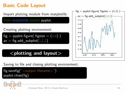
Basic Code LayoutImport plotting module from matplotlib:from matplotlib import pyplot
Creating plotting environment:fig = pyplot.figure( figsize = (4,4) )ax = fig.add_subplot(1,1,1)
<plotting and layout>
fig = pyplot.figure( figsize = (4,4) )
ax = fig.add_subplot(1,1,1)
Saving to file and closing plotting environment:fig.savefig(”<output filename>”)pyplot.close(fig)
,Christoph Menz RD II: Climate Resilience 56
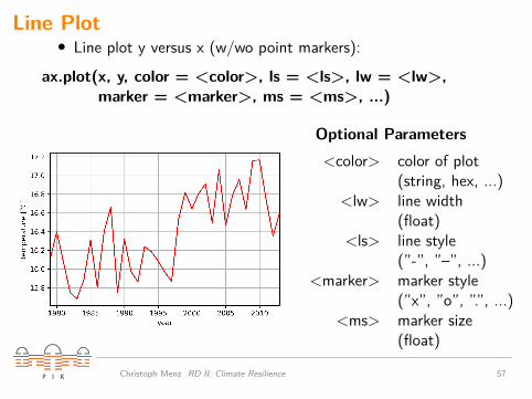
Line Plot• Line plot y versus x (w/wo point markers):
ax.plot(x, y, color = <color>, ls = <ls>, lw = <lw>,marker = <marker>, ms = <ms>, ...)
Optional Parameters<color> color of plot
(string, hex, ...)<lw> line width
(float)<ls> line style
(”-”, ”–”, ...)<marker> marker style
(”x”, ”o”, ”.”, ...)<ms> marker size
(float),
Christoph Menz RD II: Climate Resilience 57
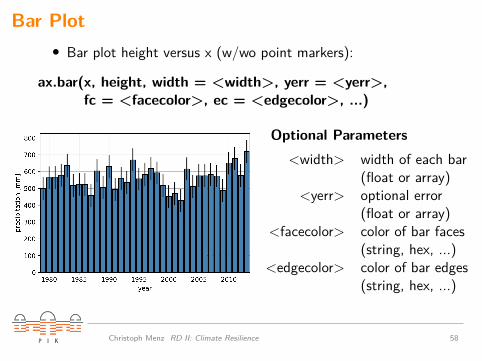
Bar Plot• Bar plot height versus x (w/wo point markers):
ax.bar(x, height, width = <width>, yerr = <yerr>,fc = <facecolor>, ec = <edgecolor>, ...)
Optional Parameters<width> width of each bar
(float or array)<yerr> optional error
(float or array)<facecolor> color of bar faces
(string, hex, ...)<edgecolor> color of bar edges
(string, hex, ...)
,Christoph Menz RD II: Climate Resilience 58
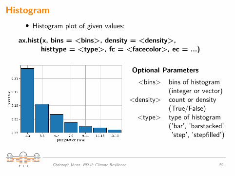
Histogram• Histogram plot of given values:
ax.hist(x, bins = <bins>, density = <density>,histtype = <type>, fc = <facecolor>, ec = ...)
Optional Parameters<bins> bins of histogram
(integer or vector)<density> count or density
(True/False)<type> type of histogram
(’bar’, ’barstacked’,’step’, ’stepfilled’)
,Christoph Menz RD II: Climate Resilience 59
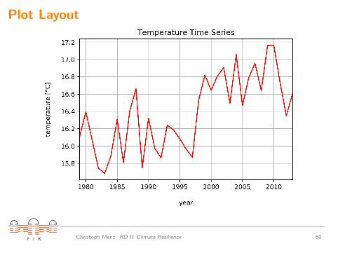
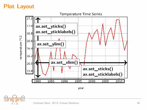
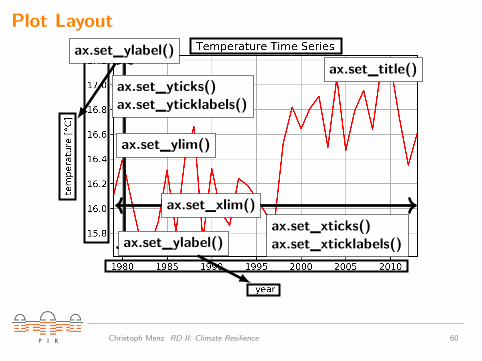
Plot Layout
ax.set_xlim()
ax.set_ylim()
ax.set_xticks()ax.set_xticklabels()
ax.set_yticks()ax.set_yticklabels()
ax.set_ylabel()
ax.set_ylabel()
ax.set_title()
,Christoph Menz RD II: Climate Resilience 60

Plot Layout
ax.set_xlim()
ax.set_ylim()
ax.set_xticks()ax.set_xticklabels()
ax.set_yticks()ax.set_yticklabels()
ax.set_ylabel()
ax.set_ylabel()
ax.set_title()
,Christoph Menz RD II: Climate Resilience 60
Plot Layout
ax.set_xlim()
ax.set_ylim()
ax.set_xticks()ax.set_xticklabels()
ax.set_yticks()ax.set_yticklabels()
ax.set_ylabel()
ax.set_ylabel()
ax.set_title()
,Christoph Menz RD II: Climate Resilience 60

Plot Layout
ax.set_xlim()
ax.set_ylim()
ax.set_xticks()ax.set_xticklabels()
ax.set_yticks()ax.set_yticklabels()
ax.set_ylabel()
ax.set_ylabel()
ax.set_title()
,Christoph Menz RD II: Climate Resilience 60
Plot Layout
ax.set_xlim()
ax.set_ylim()
ax.set_xticks()ax.set_xticklabels()
ax.set_yticks()ax.set_yticklabels()
ax.set_ylabel()
ax.set_ylabel()
ax.set_title()
,Christoph Menz RD II: Climate Resilience 60
Hands-On: Visualizationof Scientific Data with
matplotlib
,Christoph Menz RD II: Climate Resilience 61

Introduction topython-cartopy
,Christoph Menz RD II: Climate Resilience 62
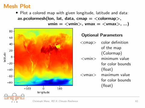
Mesh Plot• Plot a colored map with given longitude, latitude and data:ax.pcolormesh(lon, lat, data, cmap = <colormap>,
vmin = <vmin>, vmax = <vmax>, ...)
Optional Parameters<cmap> color definition
of the map(Colormap)
<vmin> minimum valuefor color bounds(float)
<vmax> maximum valuefor color bounds(float)
,Christoph Menz RD II: Climate Resilience 63
Introduction to python-cartopy
• Matplotlib can only plot raw data without referencingunderlying geographical information (no countries, no lakes,no projection, ...)
• Cartopy builds on matplotlib and implements advancedmapping features
• Developed by UK Met Office• Added features:
• Boundaries of continents, countries and states• Adding rivers and lakes to map• Adding content from shape file to map• Relate map to a projections and translate between different
projections
,Christoph Menz RD II: Climate Resilience 64
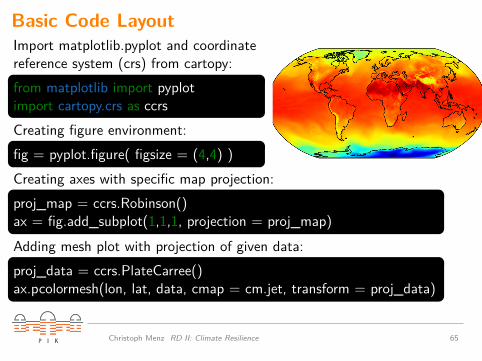
Basic Code LayoutImport matplotlib.pyplot and coordinatereference system (crs) from cartopy:from matplotlib import pyplotimport cartopy.crs as ccrsCreating figure environment:fig = pyplot.figure( figsize = (4,4) )Creating axes with specific map projection:proj_map = ccrs.Robinson()ax = fig.add_subplot(1,1,1, projection = proj_map)
Adding mesh plot with projection of given data:proj_data = ccrs.PlateCarree()ax.pcolormesh(lon, lat, data, cmap = cm.jet, transform = proj_data)
,Christoph Menz RD II: Climate Resilience 65

Projections: OverviewM
apP
roje
ctio
n
ccrs.PlateCarree() ccrs.Robinson() ccrs.Orthographic()
...
Dat
aTr
ansf
orm
atio
n Transformation between projections:
proj_cyl = ccrs.PlateCarree()proj_rot = ccrs.RotatedPole(77, 43)lon = [-170, 170, 170, -170, -170]lat = [-30, -30, 30, 30, -30]ax.fill(lon, lat, transform = proj_cyl)ax.fill(lon, lat, transform = proj_rot)
,Christoph Menz RD II: Climate Resilience 66

Adding Features to MapCartopy implements variousmap features
import cartopy.feature as cfeature
coastline = cfeature.COASTLINEborders = cfeature.BORDERSlakes = cfeature.LAKESrivers = cfeature.RIVERS
ax.add_feature(<feature>)
• Features in 3 different resolutions (110 m, 50 m and 10 m)from www.natrualearthdata.com
• External shapefiles can also be plotted
,Christoph Menz RD II: Climate Resilience 67

Colorbar• Add a colorbar to an existing map plot:
map = ax.pcolormesh(lon, lat, data)fig.colorbar(map, ax = <ax>, label = <label>,
orientation = <orientation>, ...)
Parameters<ax> parent axes
to add colorbar<label> label to add
to colorbar(string)
<orientation> colorbar orientation(”horizontal” or”vertical”)
,Christoph Menz RD II: Climate Resilience 68
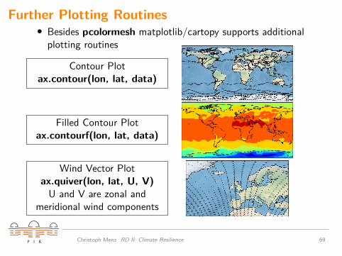
Further Plotting Routines• Besides pcolormesh matplotlib/cartopy supports additional
plotting routines
Contour Plotax.contour(lon, lat, data)
Filled Contour Plotax.contourf(lon, lat, data)
Wind Vector Plotax.quiver(lon, lat, U, V)
U and V are zonal andmeridional wind components
,Christoph Menz RD II: Climate Resilience 69

Hands-On: Visualizationof Geospatial Data with
cartopy
,Christoph Menz RD II: Climate Resilience 70
Exercise: Analysis andVisualization of netCDF
Data with python
,Christoph Menz RD II: Climate Resilience 71
Exercise
1. Create a line plot showing the annual temperature anomalytimeseries of observation and GCM model simulation of theManila grid box. The anomaly is defined as the temperatureof each year minus the average of 1981 to 2000.Hints:
• Use read_single_data() to read the data from file.• Use ilon = 12; ilat = 19 as coordinates of Manila.• Select the timeframe 1981 to 2000 using get_yindex().• Calculate the average using either np.mean() function ordata.mean() method.
• Use create_lineplot() and save_plot() to create andsave the plot.
,Christoph Menz RD II: Climate Resilience 72
Exercise
2. Create a map plot of the GCM temperature bias (for theperiod 1981 to 2000). Here the bias is defined as thedifference of the long term averages (1981 to 2000) betweenGCM simulation and observation (GCM minus observation).Hints:
• Use read_single_data() to read the data from file.• Select the timeframe 1981 to 2000 using get_yindex().• Use create_mapplot() and save_plot() to create and save
the plot.
,Christoph Menz RD II: Climate Resilience 73


![Strenghtening Capacity for Climate Change Adaptation in ... · STRENGTHENING CAPACITY FOR CLIMATE CHANGE ADAPTATION IN THE AGRICULTURE SECTOR IN ETHIOPIA] ... aims to strengthen capacity](https://static.documents.pub/doc/80x56/5ed01cafb6f1ac63cd2a298f/strenghtening-capacity-for-climate-change-adaptation-in-strengthening-capacity.jpg)
