Date post: | 05-Jun-2018 |
Category: |
Documents |
Upload: | phungtuyen |
View: | 218 times |
Download: | 0 times |
Univers
ity of
Cap
e Tow
n
Metamorphic and melt-migration history
of midcrustal migmatitic gneisses from
Nupskapa, the Maud Belt, Antarctica
Sukey Thomas
a thesis submitted for the degree of
Master of Science
at the University of Cape Town, Cape Town,
South Africa.
2014
The copyright of this thesis vests in the author. No quotation from it or information derived from it is to be published without full acknowledgement of the source. The thesis is to be used for private study or non-commercial research purposes only.
Published by the University of Cape Town (UCT) in terms of the non-exclusive license granted to UCT by the author.
Univers
ity of
Cap
e Tow
n
Plagiarism Declaration:
I know the meaning of plagiarism and declare that all the work in the document,
save for that which is properly acknowledged, is my own.
Sukey Anna Jay Thomas
15 August 2014
ii
Abstract
Melt migration is an important process in the crust that causes significant mass
transport, as well as differentiation and stabilisation of continental crust. Melt
migration near the source occurs pervasively, through interconnected networks of
melt-bearing structures. This style is restricted to the suprasolidus mid- to lower
crust, while focused migration and ascent of magma occurs in isolated dyke-
like structures under subsolidus conditions, generally in the upper crust where
brittle fracturing of rocks can occur. The details of how and when melt migration
changes from a pervasive to focused style are poorly understood, particularly
the temperature, pressure and deformation conditions which allow the transition
to occur. The Nupskapa nunatak, in Dronning Maud Land of East Antarctica,
exposes large cliffs that record evidence of multiple episodes of melt movement, in
the form of pervasive leucogranite vein networks cross-cut by larger leucogranite
dykes.
Mineral equilibria modelling with THERMOCALC and comparison of results with
previous work indicates that the Nupskapa nunatak records both Grenvillian
and Pan-African metamorphism. Coarse-grained peak assemblages in samples
from the Nupskapa area record conditions of 820–880 ◦C at 9.5–11.6 kbar, while
post-tectonic retrograde assemblages record late Pan-African conditions of 555–
595 ◦C at 3.2–4.8 kbar. These later conditions lie between the wet solidus and the
brittle-viscous transition and are inferred to represent the conditions of intrusion
for post-tectonic composite dykes.
Small-scale leucosomes predominantly lie parallel to the gneissic host rock fab-
ric and define a pervasive network across the Nupskapa cliff. These leucosomes
exhibit diffuse feathery boundaries and are inferred to represent in situ melting
and melt segregation during M1 granulite facies peak metamorphism. Compos-
ite leucogranitic dykes cross-cut both the early leucosome phase and Pan-African
shear zones in the field area. These north-trending, subvertical dykes are near-
iii
orthogonal to the gneissic fabric. They are 0.5–2 m wide and spaced ∼10–20 m
apart but not interconnected except where two dykes coalesce. The dykes show
almost no shear displacement, indicating that they formed via tensile fracture.
This indicates that their intrusion occurred during extensional or strike-slip de-
formation, under conditions of low differential stress, probably coupled to high
melt pressure. The composite dykes resulted from the far-field transport of melt
from a source 5 to 15 km below the Nupskapa outcrop. Although individually they
are discrete and focused structures, they are numerous across the field area and
closely spaced, so together they do not represent a wholly focused melt transfer
system.
The style of melt migration displayed by the composite dykes is an example of
the transition from pervasive to focused migration, occurring in the mid-crust at
subsolidus conditions. This transition involved a network of smaller melt-filled
fractures gradually coalescing into larger ones with decreasing depth. If pervasive
migration becomes focused via this gradual transition, melt accumulation and
mixing need not occur solely in the source or final emplacement structure, but
rather occurs throughout transport of the magma.
iv
Acknowledgements
I would like to thank SANAP for funding my field work in Antarctica and the
National Research Foundation for my Innovation Scholarship. Thank you to my
supervisors Johann Diener and Ake Fagereng for their guidance and assistance
and for the amazing opportunities they have provided me with. Thank you to
friends and family for their proof-reading skills and confidence in me.
v
Contents
1 Introduction 11.1 Mechanisms of melt ascent . . . . . . . . . . . . . . . . . . . . . . . . . . . . . 2
2 Geological Setting 102.1 Stratigraphy . . . . . . . . . . . . . . . . . . . . . . . . . . . . . . . . . . . . . 11
2.1.1 Jutulrøra Formation . . . . . . . . . . . . . . . . . . . . . . . . . . . . 122.1.2 Fuglefjellet and Rootshorga Formations . . . . . . . . . . . . . . . . . 122.1.3 Mafic intrusive rocks . . . . . . . . . . . . . . . . . . . . . . . . . . . . 122.1.4 Granitic intrusive phases . . . . . . . . . . . . . . . . . . . . . . . . . 13
2.2 Deformational History . . . . . . . . . . . . . . . . . . . . . . . . . . . . . . . 132.3 Metamorphic History . . . . . . . . . . . . . . . . . . . . . . . . . . . . . . . . 152.4 The Nupskapa nunatak and surrounds . . . . . . . . . . . . . . . . . . . . . . 17
2.4.1 Sveabreen Orthogneisses . . . . . . . . . . . . . . . . . . . . . . . . . . 172.4.2 Paragneisses of the Rootshorga Formation . . . . . . . . . . . . . . . . 202.4.3 Intrusive Phases . . . . . . . . . . . . . . . . . . . . . . . . . . . . . . 22
3 The Nupskapa Outcrop 233.1 Lithologies and fabrics . . . . . . . . . . . . . . . . . . . . . . . . . . . . . . . 243.2 Leucogranite Phases . . . . . . . . . . . . . . . . . . . . . . . . . . . . . . . . 27
3.2.1 Stromatic leucosome . . . . . . . . . . . . . . . . . . . . . . . . . . . . 273.2.2 Injected pervasive network . . . . . . . . . . . . . . . . . . . . . . . . . 273.2.3 Composite dykes . . . . . . . . . . . . . . . . . . . . . . . . . . . . . . 283.2.4 Pegmatitic phase . . . . . . . . . . . . . . . . . . . . . . . . . . . . . . 31
4 Petrography and Mineral Chemistry 334.1 Petrography . . . . . . . . . . . . . . . . . . . . . . . . . . . . . . . . . . . . . 34
4.1.1 Mafic Samples . . . . . . . . . . . . . . . . . . . . . . . . . . . . . . . 344.1.2 Metapelitic Samples . . . . . . . . . . . . . . . . . . . . . . . . . . . . 38
4.2 Mineral Chemistry . . . . . . . . . . . . . . . . . . . . . . . . . . . . . . . . . 414.2.1 Mafic Samples . . . . . . . . . . . . . . . . . . . . . . . . . . . . . . . 414.2.2 Metapelitic Samples . . . . . . . . . . . . . . . . . . . . . . . . . . . . 50
4.3 Inferred equilibrium assemblages . . . . . . . . . . . . . . . . . . . . . . . . . 554.3.1 Mafic Samples . . . . . . . . . . . . . . . . . . . . . . . . . . . . . . . 554.3.2 Metapelitic Samples . . . . . . . . . . . . . . . . . . . . . . . . . . . . 56
5 Mineral Equilibria Modelling 575.1 Methodology . . . . . . . . . . . . . . . . . . . . . . . . . . . . . . . . . . . . 575.2 Results . . . . . . . . . . . . . . . . . . . . . . . . . . . . . . . . . . . . . . . . 59
5.2.1 Mafic Samples . . . . . . . . . . . . . . . . . . . . . . . . . . . . . . . 59
vi
5.2.2 Metapelitic Samples . . . . . . . . . . . . . . . . . . . . . . . . . . . . 65
6 Discussion 706.1 Estimation of peak and retrograde P-T conditions . . . . . . . . . . . . . . . 70
6.1.1 Mafic Samples . . . . . . . . . . . . . . . . . . . . . . . . . . . . . . . 706.1.2 Summary of metamorphic conditions recorded by mafic samples . . . 716.1.3 Summary of conditions recorded by metapelitic samples . . . . . . . . 72
6.2 Likely P-T paths and comparisons with previous work . . . . . . . . . . . . . 726.3 Inferred style of melt migration . . . . . . . . . . . . . . . . . . . . . . . . . . 766.4 Implications for far-field melt transfer . . . . . . . . . . . . . . . . . . . . . . 836.5 Conclusions . . . . . . . . . . . . . . . . . . . . . . . . . . . . . . . . . . . . . 85
References 87
A Electron microprobe tables 94
vii
List of Tables
4.1 Mineral names and abbreviations used in this study, as used in THERMOCALC. 334.2 Representative mineral compositions for sample S33 . . . . . . . . . . . . . . 434.3 Representative mineral compositions for sample S53 . . . . . . . . . . . . . . 454.4 Representative mineral compositions for sample S65 . . . . . . . . . . . . . . 474.5 Representative mineral compositions for sample S67 . . . . . . . . . . . . . . 514.6 Representative mineral compositions for sample S62 . . . . . . . . . . . . . . 534.7 Representative mineral compositions for sample S64 . . . . . . . . . . . . . . 54
5.1 XRF whole-rock analyses of selected samples . . . . . . . . . . . . . . . . . . 585.2 Bulk compositions (in mol %) used to construct pseudosections . . . . . . . . 59
A.1 Electron microprobe results for garnet in all samples . . . . . . . . . . . . . . 95A.2 Electron microprobe results for amphibole . . . . . . . . . . . . . . . . . . . . 101A.3 Electron microprobe results for pyroxenes . . . . . . . . . . . . . . . . . . . . 117A.4 Electron microprobe results for feldspars . . . . . . . . . . . . . . . . . . . . . 120A.5 Electron microprobe results for biotite . . . . . . . . . . . . . . . . . . . . . . 136A.6 Electron microprobe results for Muscovite . . . . . . . . . . . . . . . . . . . . 146A.7 Electron microprobe results for Sillimanite . . . . . . . . . . . . . . . . . . . . 148
viii
List of Figures
1.1 Illustration of fracture system . . . . . . . . . . . . . . . . . . . . . . . . . . . 4
2.1 Geological map of western Antarctica . . . . . . . . . . . . . . . . . . . . . . 112.2 P-T-t histories for H.U Sverdrupfjella as identified by different researchers . . 162.3 Geological map of Nupskapa field are . . . . . . . . . . . . . . . . . . . . . . . 182.4 Example of Nupskapa orthogneiss . . . . . . . . . . . . . . . . . . . . . . . . 192.5 Example of Nupskapa paragneiss . . . . . . . . . . . . . . . . . . . . . . . . . 202.6 Example of a mafic lens . . . . . . . . . . . . . . . . . . . . . . . . . . . . . . 21
3.1 Other outcrops showing similar intrusive phases . . . . . . . . . . . . . . . . . 243.2 Stereonet showing orientation of cliff foliation . . . . . . . . . . . . . . . . . . 253.3 The Nupskapa Cliff . . . . . . . . . . . . . . . . . . . . . . . . . . . . . . . . . 263.4 Close-up of stromatic leucosome phase . . . . . . . . . . . . . . . . . . . . . . 273.5 Close-ups of the primary pervasive melt and composite dyke phases . . . . . 283.6 Stereonet showing orientations of composite dykes . . . . . . . . . . . . . . . 293.7 Close-up photograph of two narrower dykes joining . . . . . . . . . . . . . . . 293.8 Composite dyke cross-cutting a shear zone . . . . . . . . . . . . . . . . . . . . 303.9 The different phases making up the composite dykes . . . . . . . . . . . . . . 313.10 Stereonet showing orientations of the pegmatitic phase dykes . . . . . . . . . 323.11 Pegmatitic phase exploiting fabric . . . . . . . . . . . . . . . . . . . . . . . . 32
4.1 Field area with sample locations indicated . . . . . . . . . . . . . . . . . . . . 344.2 Thin section textures of S33 . . . . . . . . . . . . . . . . . . . . . . . . . . . . 354.3 Thin section texture of S53 . . . . . . . . . . . . . . . . . . . . . . . . . . . . 364.4 Thin section textures of S65 . . . . . . . . . . . . . . . . . . . . . . . . . . . . 374.5 Thin section textures of S67 . . . . . . . . . . . . . . . . . . . . . . . . . . . . 384.6 Thin-section texture in S62 showing fine muscovite . . . . . . . . . . . . . . . 394.7 Thin-section texture in S62 showing coarse muscovite . . . . . . . . . . . . . 394.8 Thin-section textures in S64 showing sillimanite . . . . . . . . . . . . . . . . . 404.9 Thin-section textures in S64 showing layering . . . . . . . . . . . . . . . . . . 404.10 Graph to show distribution of Al and Na in hornblende grains in S33 . . . . . 424.11 Graph to show distribution of feldspar compositions in S33 . . . . . . . . . . 424.12 Feldspar compositions in S53 . . . . . . . . . . . . . . . . . . . . . . . . . . . 444.13 Al(VI) and Na in amphibole grains in S65 . . . . . . . . . . . . . . . . . . . . 464.14 Plagioclase compositions in S65 . . . . . . . . . . . . . . . . . . . . . . . . . . 484.15 Graph showing Al and Ti in biotite grains in S65 . . . . . . . . . . . . . . . . 484.16 Al and Na in amphibole grains in S67 . . . . . . . . . . . . . . . . . . . . . . 494.17 Feldspar compositions in S67 . . . . . . . . . . . . . . . . . . . . . . . . . . . 504.18 Graph to show distribution of feldspar compositions in S62. . . . . . . . . . . 52
ix
4.19 Graph to show distribution of feldspar compositions in S64. . . . . . . . . . . 52
5.1 Calculated pseudosection for S65 . . . . . . . . . . . . . . . . . . . . . . . . . 605.2 Calculated pseudosection for S67 . . . . . . . . . . . . . . . . . . . . . . . . . 625.3 Calculated pseudosection for S33 . . . . . . . . . . . . . . . . . . . . . . . . . 635.4 Calculated pseudosection for S53 . . . . . . . . . . . . . . . . . . . . . . . . . 655.5 Calculated pseudosection for the residuum composition of S62 . . . . . . . . . 665.6 Calculated pseudosection for the rehydrated composition of S62 . . . . . . . . 675.7 Calculated pseudosection for the residuum composition of S64 . . . . . . . . . 685.8 Calculated pseudosection for the rehydrated composition of sample S64 . . . 69
6.1 Overlapping the stable assemblage fields . . . . . . . . . . . . . . . . . . . . . 736.2 Pan-African P-T path . . . . . . . . . . . . . . . . . . . . . . . . . . . . . . . 746.3 Polymetamorphic . . . . . . . . . . . . . . . . . . . . . . . . . . . . . . . . . . 746.4 Comparison of Nupskapa P-T conditions with other work . . . . . . . . . . . 756.5 An idealised crustal-scale melt migration network . . . . . . . . . . . . . . . . 84
x
Chapter 1
Introduction
Granitic melt migration is an important process in the Earth’s continental crust. It causes
significant mass transport, as well as differentiation and stabilisation of continental crust
(Sawyer, 1994; Brown & Solar, 1998a; Bons et al., 2004; Brown, 2004, 2010; Sawyer et al.,
2011). The presence of even a low melt fraction can significantly weaken the continental crust,
and therefore has important consequences for how deformation and orogenic events occur
(Brown, 1994; Brown & Solar, 1998a; Vigneresse, 2006; Schulmann et al., 2008; Beaumont
et al., 2009; Brown, 2010; Sawyer et al., 2011; Jamieson & Beaumont, 2011)
Granitic melt forms in the lower crust through partial melting of extensive volumes of
rock (Stevens et al., 1997; Vielzeuf & Schmidt, 2001). How much melt forms depends on
the rock type, the temperature and pressure at which melting occurs, and the hydrous fluid
content of the source rocks (Clemens & Vielzeuf, 1987; Stevens et al., 1997; Vigneresse, 2006).
Melt forms in the lower crust at depths anywhere between 20 and 70 km (but on average at
∼30 km; Brown et al., 2011; Sawyer et al., 2011), with large volumes of rock producing melt
dispersed along grain boundaries (i.e. millimetre to submillimetre scale) (Vigneresse, 2006).
Melt emplaces in the upper crust as discrete plutonic bodies (up to tens of kilometres in
size) in the upper crust, at ∼10 km depth, or may erupt as lava (Brown et al., 2011; Sawyer
et al., 2011). Thus melt must accumulate into larger volumes and migrate through the crust,
before being emplaced in the upper crust. On its way through the crust melt must move
through country rocks at suprasolidus conditions, into shallower country rock at subsolidus
conditions and, in some instances, cross the brittle-viscous transition(Sawyer et al., 2011); all
without crystallising. The solidus represents the transition from melt-bearing to melt-absent
rocks, and the brittle-viscous transition represents the change from distributed to localised
1
deformation of the country rock. Thus, both form major rheological boundaries and rocks
on either side will respond very differently to deformation (Brown & Solar, 1999; Vigneresse,
2006; Brown, 2010; Sawyer et al., 2011). It is therefore unlikely that melt can move from the
lower to upper crust via one mechanism that is capable of overcoming all of these rheological
changes (Clemens & Mawer, 1992; Paterson & Fowler, 1993; Brown, 1994; Weinberg, 1996).
Melt migration is generally thought to occur via one (or a combination) of two end-member
mechanisms, which operate in different parts of the crust: pervasive flow in the lower, hotter
parts of the crust (see Collins & Sawyer, 1996; Weinberg, 1999; Bons et al., 2004; Hall &
Kisters, 2012), and focused flow in the upper, cooler parts of the crust (see Clemens &
Mawer, 1992; Brown, 1994; Weinberg, 1996; Clemens et al., 1997; Petford et al., 1994). The
conditions and processes by which one mechanism transforms to the other have not been
resolved (e.g. Brown & Solar, 1998a). This project aims to address some of these issues,
in particular: by what mechanisms, and under what pressure, temperature and deformation
conditions melt moves through the mid-crust, as well as how and when the style of movement
changes from pervasive to focused.
1.1 Mechanisms of melt ascent
There are three main end-member models of how melt ascent can take place:
1. Diapirism involves the gradual rising of buoyant magma as large single volumes. Duc-
tile deformation in the hot surrounding rock controls the rate of ascent (Bons et al.
(2004) and others therein). Up until the early 1990s, this was the preferred mechanism
of ascent for granitic melt (Sweeney, 1975; Marsh, 1982; Bateman, 1984). Many re-
searchers (e.g. Clemens & Mawer, 1992; Brown, 1994; Weinberg, 1996; Clemens et al.,
1997; Bons et al., 2004) now agree that evidence for frequent diapirism in the crust
is lacking, and consider it to be an unfeasible explanation for the ascent of melt and
emplacement of most plutons and magma chambers in the upper crust. Others (e.g
Weinberg & Podladchikov, 1994) regard it as a suitable explanation for the ascent
and emplacement of plutons in the lower crust. In particular, the emplacement of the
well-studied Sierra Nevada batholith is thought to have involved diapirism, as well as
other mechanisms such as fracturing (Paterson & Vernon, 1995; McNulty et al., 2000).
Extensive computer modelling by Mahon et al. (1988), based on calculating an ascent
velocity relationship for granitoid diapirs and applying this to a heat flow model within
2
the crust, has shown that despite varying the magma volume, temperature, starting
depth and density contrast between diapir and country rock, and irrespective of likely
changes in geothermal gradient, diapiric granitic magma bodies eventually crystallize
and do not emplace higher than the mid-crust. Because diapirism is thought to occur
only under very specific circumstances, it will not be considered further in this study.
2. Focused flow involves the ascent of magma via a limited number of conduits, such as
conventional dykes, self-propagating fractures and crustal-scale shear zones (Weertman,
1971; Sleep, 1988; Lister & Kerr, 1991; Clemens & Mawer, 1992; Petford et al., 1993;
Brown, 1994; Petford et al., 1994; Weinberg, 1996; Clemens et al., 1997; Bons et al.,
2004; Hall & Kisters, 2012). It was known as a mechanism for the transport of mafic
magmas (e.g Weertman, 1971), and researchers were doubtful as to its application to
granitic magmas, owing to the much lower viscosity contrast between granitic magma
and country rocks. However, it has since been shown that granitic magmas can also
ascend via dyke structures and that this is an efficient mechanism of transporting large
volumes of melt through subsolidus crust (Clemens & Mawer, 1992; Petford et al., 1993;
Brown & Solar, 1999; Hall & Kisters, 2012).
Focused flow may occur via brittle mechanisms, where fracturing occurs as a result of
melt pressure building up sufficiently to overcome the tensile strength of the rock at
the fracture tip, creating a path along which melt can then move (Sleep, 1988; Petford,
1996; Brown, 2004; Weinberg, 1999; Kisters et al., 2009). This results in dykes and/or
self-propagating fractures.
The aspect ratio (i.e. width verses length) of a dyke or self-propagating fracture is
a function of effective normal stress and tensile strength (Clemens & Mawer, 1992;
Vermilye & Scholz, 1995). This aspect ratio is thus limited by gradients in effective
normal stress as a result of the differing rates of increase between lithostatic pressure and
melt pressure with depth, and is also limited by the tensile stress caused by melt pressure
and therefore by melt-supply (Weertman, 1971). If a melt-filled fracture exceeds its
maximum length (on the order of several tens to hundreds of metres), or if melt supply is
insufficient to keep the dyke open, it may start to close on one end while simultaneously
opening on the other (Clemens & Mawer, 1992; Weinberg, 1999; Bons et al., 2001,
2004; Kisters et al., 2009). Melt is then envisaged as moving through these ‘mobile’
fractures as individual pulses, controlled by the supply of magma in the source region.
3
In subduction zones, these pulses are thought to be frequent and of small volume, as
less-frequent, larger volumes would require more storage time in larger crustal reservoirs
(Brown, 2004). Because the fracture closes up after the individual batch of melt has
passed through, this mechanism may leave little evidence behind in exposed outcrops,
with dykes appearing much thinner after having been almost totally drained of melt
(Clemens & Mawer, 1992; Petford et al., 1994; Weinberg, 1999; Bons et al., 2008; Brown,
2004).
It is thought that smaller melt-filled fractures gradually coalesce into larger fractures,
creating a self-similar system, which eventually drains into crustal-scale features ((Fig-
ure 1.1; Weinberg, 1999; Bons et al., 2004; Sawyer et al., 2011). These large features are
then able to drain the source and transport a large volume of magma through a small
number of individual structures (Weinberg, 1996; Bons et al., 2004; Brown, 2004).
Figure 1.1: Schematic illustration of the way in which melt-filled fractures are thought to
gradually coalesce into larger fractures, creating a self-similar system. The larger fractures
drain into crustal-scale features such as large dykes and shear zones. (After Faber, 2012)
Focused flow may also occur via ductile or strain-controlled mechanisms. Owing to
the anisotropic nature of the lower crust, the anatectic region is unlikely to be a simple
tabular horizontal section of the crust. Similarly, it is likely that sections of the anatectic
zone will be inclined to one of the principal stresses and thus shear stresses will operate
4
across that section. Melt-filled fractures experiencing shear stresses will deform more
easily than the surrounding melt-free rock. This leads to the development of melt-
lubricated shear zones (Hollister & Crawford, 1986; Brown & Solar, 1998a,b, 1999;
Handy et al., 2001). Dykes may initiate in suprasolidus crust through ductile fracture
but, during ascent through increasingly viscous subsolidus crust, this ductile fracture
process may change to a brittle-elastic fracture process (Weinberg & Regenauer-Lieb,
2010; Brown et al., 2011; Brown, 2013).
It has been shown that melt migration via this method, in discrete structures that are on
the order of a few metres wide, is an efficient process that allows for the transport of large
volumes of magma through the subsolidus crust, at rapid rates, to the emplacement
level in the upper crust (Clemens & Mawer, 1992; Petford et al., 1993, 1994; Rubin,
1995; Petford, 1996).
The regional stress regime operating in the crust during magma ascent will greatly
influence the style of focused flow, particularly the deformation mechanism but also the
shape and orientations of the fractures or melt-ascent-features (Petford, 1996; Weinberg,
1996). Conventional (vertical) dyking as an ascent mechanism may be inhibited in
convergent orogenies, for instance, as fractures generally form parallel to maximum (and
normal to minimum) compressive stress (Anderson, 1951; Brown, 1994; Vanderhaeghe,
2001; Vigneresse, 2006). Assuming Andersonian mechanics, this means that dykes in
convergent orogenies will be horizontal, normal to a vertical σ3. Thus melt will migrate
laterally in fractures and dykes but upward movement of melt will be inhibited. In
such a case it is more likely that melt will ascend via crustal-scale shear zone structures
(Clemens & Mawer, 1992; Brown, 1994; Brown & Solar, 1998b).
In order for dyking to initiate and operate, the surrounding rock must be brittle, at
least momentarily and locally at the fracture tip, as rock behaving viscously will flow
instead of fracturing, thus dissipating the fracture propagation energy (Clemens &
Mawer, 1992). Brittle failure by tensile fracture is possible in rocks in the anatectic
zone if the melt pressure is larger than the combination of the tensile strength of the
rocks and the least compressive stress. This required melt pressure will increase with
depth because of increases in confining stress, resulting in larger melt pressures being
required to initiate fractures. Under the high temperature conditions of the lower crust,
rocks will be more likely to flow viscously before this large required melt pressure is
5
reached. If enough melt pressure does build up to cause hydraulic fracturing, that melt
pressure is soon dissipated and will take a while to build up again. This may lead to
melt being transported via discrete pulses or batches (e.g. Bons et al., 2004), but will
not result in continuous melt flow from the source to the upper crust (Brown, 1994).
Thus, the formation of dykes that transport large volumes of magma vertically upwards
is most likely limited to the higher subsolidus parts of the crust as their formation and
propagation is inhibited in the lower, high-pressure crust (Clemens & Mawer, 1992;
Petford et al., 1994; Bons et al., 2004).
3. Pervasive melt migration envisages melt moving through interconnected permeability
or fracture systems (Collins & Sawyer, 1996; Weinberg, 1999; Vanderhaeghe, 2001;
Leitch & Weinberg, 2002; Bons et al., 2004; Weinberg & Regenauer-Lieb, 2010; Hall
& Kisters, 2012). The movement of magma in these pervasive networks is thought
to be driven by local pressure gradients caused by tectonic deformation (and in some
instances buoyancy), and operates efficiently in rocks at suprasolidus conditions (Brown,
1994; Weinberg, 1999). Deformation of anisotropic crust leads to the development of
pressure gradients and structural heterogeneities on all scales. These pressure gradients
cause melt to move towards sites of low pressure (Brown, 1994; Sawyer, 1994; Collins
& Sawyer, 1996; Brown & Solar, 1999). Thus melt exploits existing anisotropies and
dilatancy sites such as layering, foliation planes, fold hinges, mineral lineation and
boudin necks (Brown, 1994; Collins & Sawyer, 1996; Weinberg, 1999).
The orientation of dilational sites depends on the orientation of the principal stresses
and on the orientation of pre-existing anisotropies, which may vary depending on when
they formed, as they may have formed in a separate deformation phase (Sawyer et al.,
2011; Hall & Kisters, 2012; Reichardt & Weinberg, 2012). Thus, the dilational sites and
existing anisotropies that melt exploits may commonly be subhorizontal, and so melt
may experience extensive lateral migration before any vertical ascent occurs (Brown,
1994). In the absence of a pressure gradient, if melt volume is locally very high, or if
the strain rate caused by deformation is greater than the rate at which melt can move
to low-pressure sites, melt pressure can increase, reducing effective normal stress and
causing hydraulic fracturing of the country rock (Clemens & Mawer, 1992; Brown, 1994;
Weinberg, 1999; Hall & Kisters, 2012).
Because the small melt bodies making up the pervasive network are susceptible to solidi-
6
fication as a result of heat loss, melt migration may cease if the thermal contrast between
melt and country rock becomes too large. Pervasive flow is therefore generally limited
to hotter parts of the crust, usually to the level of the crustal isotherm corresponding
to the solidus of the melt (Brown & Solar, 1998a; Weinberg, 1999). Thus, pervasive
flow generally occurs within, or close to, the anatectic region (Weinberg, 1999; Brown,
2004; Hall & Kisters, 2012). However, the limits of pervasive flow may be extended to
shallower levels in the crust through feedback relationships between melt migration and
thermal structure (Weinberg, 1996; Brown & Solar, 1998a; Weinberg, 1999). Once melt
has been removed from its source, the remaining volume of rock will be less fertile and
so will have an elevated solidus (White & Powell, 2002). Thus, segregated melt tends to
have a lower solidus temperature than the rocks it formed from (sometimes by as much
as 100◦C; Weinberg, 1999), and so can migrate away from its source before freezing.
The movement of melt up through the crust allows heat to be transferred to shallower
crustal levels, moving isotherms higher and allowing melt to migrate further before it
freezes, thus extending the limits of pervasive migration (Brown & Solar, 1999). With
favourable conditions, the zone of pervasive melt migration may be extended above
the anatectic zone, by about 3–5 km (Weinberg, 1999; Faber, 2012). Controls such as
rate of melt production and extraction, as well as the rate of heat advection, will cause
pervasive flow to eventually cease operating and thus, pervasive flow cannot account
for large volumes of magma intruded into colder and/or shallower levels of the crust
(Weinberg, 1999; Leitch & Weinberg, 2002).
Pervasive flow occurs via a dispersed network of many small centimetre- to metre-scale
structures, whereas focused flow operates via fewer, separated structures, on the order of a
few metres in width, and up to several hundreds of metres high. Pervasive migration occurs
in the lower crust, where melt is formed, whereas focused flow operates in the upper crust
where melt is emplaced (Weinberg, 1999; Sawyer et al., 2011). Both of these melt migration
mechanisms are greatly inhibited under the conditions at which the other operates. However,
melt is able to ascend through the crust and so there must be some depth in the crust at
which the mechanism of melt ascent changes from a pervasive network and instead occurs in
fewer, discrete, focused structures.
The details of how and when pervasive flow changes to focused flow are poorly con-
strained. Specifically, little is known about the mechanisms that might result in the linking
7
of distributed melt-bearing networks, close to the anatectic region, to larger discrete bodies
that allow melt ascent through subsolidus crust. (Brown & Solar, 1998a,b; Weinberg, 1999;
Connolly & Podladchikov, 2007; Hall & Kisters, 2012; Brown, 2013).
Bons et al. (2004) produced a numerical model to investigate stepwise segregation and
accumulation of melt batches during progressive melting of a source region. Instead of a
discrete point at which one migration style changes to another, their model explained melt
movement as occurring, from initial segregation into centimetre-scale leucosomes to far-field
melt transfer and emplacement, via one holistic system of mobile hydrofractures. This self-
similar fracture system, as illustrated in Figure 1.1, is thought to link the pervasive network
with the larger dykes or shear zones that eventually feed plutons. Ito & Martel (2002) per-
formed laboratory experiments and numerical calculations in order to investigate how dykes
may coalesce owing to interactions with the local stress field. They found that neighbouring
dykes create distortions in the local stress field that can be attractive or repulsive according
to vertical and horizontal spacing. Two adjacent dykes will tend to merge as they interact,
if they are spaced closely enough to each other. However, their study was more applicable
to the low-viscosity asthenosphere below mid-ocean ridges, and the possibility of a similar
situation operating in the continental crust was not evaluated. Weinberg & Regenauer-Lieb
(2010) suggested dyking by ductile fracturing as a mechanism for melt extraction from rocks
with a low melt fraction. These ductile fractures would have blunt tips and irregular mar-
gins. If they were to grow large enough, they might have sufficient buoyancy to overcome the
fracture toughness at their tips, or could transport melt to cooler and more competent parts
of the crust where brittle-elastic dyking could take over. In this way, brittle-elastic dykes
may have their origins as ductile fracture dykes in the hotter regions of the crust. While this
model was only valid for pure-shear systems, it does appear to corroborate, to some extent,
the ‘one holistic system’ of Bons et al. (2004).
Diener et al. (2014) described an example of melt segregation and substantial melt accu-
mulation occurring in the near-source region, allowing larger volumes of melt to accumulate.
This substantial melt accumulation implies that the change from a pervasive to focused melt
migration mechanism can happen in the source rather than higher in the crust (Rubin, 1995;
Diener et al., 2014).
Morfin et al. (2013) described an example where melt migrated into a near-solidus region,
with injection occurring along thin dykes parallel to the existing bedding or foliation planes.
The melt was never channelled into larger structures capable of transporting melt through
8
the crust, and so the near-source region instead forms an injection complex.
Faber (2012) described an example where pervasive melt migration occurred in rocks
above the solidus, and operated as an effective mechanism of melt migration beyond the
source region and through the suprasolidus mid-crust. Faber (2012) also acknowledged the
limitations of pervasive migration, to about 3-5 km above the source region, as well as the
need for the pervasive network to become amalgamated into the larger structures that feed
plutons. Faber (2012) suggested that melt migration was a pervasive process, and involved
networks of dykes throughout the crust that become less interconnected and less numerous
towards shallower levels, much like the model suggested by Bons et al. (2004).
The various models of how pervasive flow changes to focused flow lack consensus, and more
descriptions of exhumed field examples are needed. Furthermore, the temperature, pressure
and deformation conditions, which allow pervasive flow to become more focused, are poorly
understood. This project will attempt to address these questions, through the investigation of
well-exposed mid-crustal rocks that exhibit a style of melt-migration that contains aspects of
both pervasive and focused mechanisms. These rocks are exposed at Nupskapa in Dronning
Maud Land, Antarctica, and form part of the polymetamorphic Maud Belt that joins the
Grunehogna craton with the central cratonic block (or ‘Mawson Continent’) of Antarctica
(Fitzsimons, 2000a).
This study examines the petrography of several samples taken from the Nupskapa area
in order to identify the different mineral assemblages preserved in the samples. The textures
of minerals in each sample are examined to better identify equilibrium mineral assemblages.
Mineral chemistry of individual samples, determined using an electron microprobe, are anal-
ysed in terms of compositional variations both across the sample and within individual min-
eral grains. This provides insight into how minerals re-equilibrated as a response to changes
in pressure and temperature experienced by the rocks. Both the petrographic and mineral
chemistry studies are combined with the results of mineral equilibria modelling, through
the program THERMOCALC, to determine the P-T history recorded by the rocks in the
Nupskapa area, specifically, the metamorphic conditions under which the composite dykes
intruded. The geometry and orientations of the leucogranitic dykes and host-rock fabric are
also described. This provides insight into the deformational conditions under which the dykes
intruded, and allows description of the physical conditions of this style of melt migration.
9
Chapter 2
Geological Setting
The East Antarctic Shield is made up of several Archaean cratonic nuclei, separated by
polydeformed mobile belts that preserve evidence of complex metamorphic and deformation
histories (Figure 2.1; Fitzsimons, 2000a; Board, 2001). Two major tectonothermal episodes
are recorded in the high-grade gneisses of the polymetamorphic Maud Belt. The first, at
∼1300 to 900 Ma, corresponds to the Grenvillian event and the amalgamation of the Rodinia
supercontinent, and involved high-grade metamorphism accompanied by major tectonism
(Groenewald & Hunter, 1991; Grantham et al., 1995). The second, at ∼600 Ma to ∼450 Ma,
corresponds to the Pan-African event and the amalgamation of Gondwana and was originally
thought to have involved heating with little associated deformation (e.g Groenewald et al.,
1991; Grantham et al., 1995) but is now interpreted to have also involved significant tectonism
(Fitzsimons, 2000a; Board et al., 2005; Bisnath & Frimmel, 2005).
The high-grade Maud Belt lies along the southern edge of the Grunehogna Province, an
Antarctic fragment of the Kaapvaal-Zimbabwe craton (Fitzsimons, 2000a). The belt stretches
for over 700 km northeast-southwest (Figure 2.1). It is composed of upper amphibolite-
to granulite-facies supracrustal rocks of the Sverdrupfjella Group that experienced multiple
phases of deformation from the Mesoproterozoic to early Cambrian, as well as several pre-,
syn- and post-tectonic intrusions, mostly granitic or mafic in composition (Groenewald et al.,
1995; Paulsson & Austrheim, 2003; Bisnath et al., 2006). The belt is made up of several
different geographic sections which have been studied to varying degrees. From southwest
to northeast they are: Heimefrontfjella, Kirwanveggen and H.U. Sverdrupfjella. Further east
of H.U. Sverdrupfjella are the Gjelsvikfjella, Muhlig-Hofmannfjella and Central Dronning
Maud Land sections. Correlation between the different sections can be problematic owing
10
Figure 2.1: Geological map of western Antarctica, with field area indicated. After Board
et al. (2005)
to the lack of outcrop in between. H.U. Sverdrupfjella, lying between the Kirwanveggen
and Gjelsvikfjella ranges in the central part of the Maud Belt, represents one of the more
thoroughly-studied sections (Grantham et al., 1995; Groenewald et al., 1995; Board et al.,
2005) and forms the focus of this study.
2.1 Stratigraphy
Several different stratigraphic subdivisions have been proposed for the rocks of the H.U.
Sverdrupfjella area (e.g. Grantham & Hunter, 1988). The subdivisions used here are those of
Hjelle (1974) as modified by Groenewald et al. (1995) and Board et al. (2005).
The gneisses of the Sverdrupfjella Group are made up of both amphibolite-facies assem-
blages and partially retrogressed granulites (Hjelle, 1974; Groenewald et al., 1995; Grantham
11
et al., 1995; Board et al., 2005). The relative proportions of these different rock types varies
from area to area.
2.1.1 Jutulrøra Formation
The gneisses of the Jutulrøra Formation form most of the outcrop in the western section
of H.U. Sverdrupfjella, and show U–Pb zircon ages of 1160–1140 Ma (Arndt et al., 1991;
Groenewald et al., 1995; Paulsson & Austrheim, 2003; Board et al., 2005; Bisnath et al.,
2006). This formation is made up of tonalitic gneisses intercalated with banded mafic to
felsic ortho- and paragneisses. These, together with the oldest intrusive rocks that preserve
ages of 1140–1130 Ma, are thought to represent part of a larger Mesoproterozoic volcanic arc
system (Groenewald et al., 1995; Bisnath et al., 2006).
2.1.2 Fuglefjellet and Rootshorga Formations
The eastern and southeastern sections of H.U. Sverdrupfjella comprise the Fuglefjellet and
Rootshorga Formations. The former (and structurally lower) is a sequence of predominantly
carbonates intercalated with quartzofeldspathic, calc-silicate, magnesian and mafic rocks
(Groenewald et al., 1995; Board et al., 2005). The Rootshorga Formation makes up most of
the eastern H.U. Sverdrupfjella and shows more diversity in composition, containing pelitic
to quartzofeldspathic paragneiss and intermediate to felsic orthogneiss, with minor zones of
mafic and calc-silicate composition (Board, 2001). A sedimentary origin is indicated for this
formation by the gradational compositional variations, banding on a metre scale and inter-
layering of gneisses derived from pelites, greywackes, conglomerates, diamictites and arenites
(Groenewald et al., 1995; Board et al., 2005). The Fuglefjellet and Rootshorga Formations
together are inferred to represent a retro-arc marginal basin succession (Groenewald et al.,
1995)
2.1.3 Mafic intrusive rocks
Intrusive mafic rocks occur throughout the Sverdrupfjella Group, usually as lenses, boudins
and isolated layers within gneisses. They vary in composition, including gabbro, pyroxenite,
olivine gabbronorite and dunite. They are mostly pretectonic, with the interior of the lenses
or boudins protected from the gneissic foliation which anastomoses around the mafic lenses
(Groenewald et al., 1995; Board, 2001). Several Jurassic dolerite dykes are found in the H.U.
12
Sverdrupfjella area, and are related to the breakup of Gondwana (Harris & Grantham, 1993;
Groenewald et al., 1995; Board, 2001).
2.1.4 Granitic intrusive phases
Multiple phases of early (relating to the Grenvillian orogeny) leucogranitic intrusions are
found in H.U. Sverdrupfjella. Harris et al. (1995) identified early tabular granite bodies
(1103 ± 17 Ma; Harris et al., 1995) as well as garnet-biotite granites (1131 ± 25 Ma; Harris
et al., 1995). Various generations of smaller leucogranitic bodies are also found across the
area (Board et al., 2005). The various age relations can be difficult to correlate between
localised areas but there appears to be a progressive change in the melt compositions over
time. They show a progressive change from early near minimum melt compositions to decom-
pression melts, and finally to volcanic arc types which may represent second-stage melting of
subducted rocks.This is characteristic of an extended period of collisional tectonics, possibly
followed by second-stage melting of subducted rocks leading to the formation of a volcanic
arc (Groenewald et al., 1995).
The Sveabreen gneissic granites described by Groenewald et al. (1995) extend through-
out the eastern and south-eastern H.U. Sverdrupfjella, where they are intercalated with the
Rootshorga Formation through a series of thrusts (Board et al., 2005). These gneissic gran-
ites are megacrystic and show S-type characteristics, with garnet and sillimanite present in
isolated areas. Groenewald et al. (1995) interpreted the Sveabreen granites as having an early
syn-tectonic origin. They have been dated at 1061 ±14 Ma by Harris et al. (1995).
Younger, post-tectonic intrusions found in the H.U. Sverdrupfjella area include the Brattskarvet
Intrusive Suite, which comprises alkaline to peralkaline A-type granites, thought to have re-
sulted from a major heating event between ∼550 and 450 Ma(Grantham et al., 1995; Groe-
newald et al., 1995; Board et al., 2005) as well as abundant monzogranitic dykes and veins,
which show ages of 469 ± 5 Ma (Board (2001); after Grantham (1992)).
2.2 Deformational History
The two orogenic events recorded in the H.U. Sverdrupfjella area have near-identical kine-
matic expressions. They both appear to have resulted in the formation of shallowly-dipping
fabrics and top-to-the-NW shear-sense indicators. Discriminating between the structures
and fabrics of the two orogenic periods is therefore challenging and somewhat controversial
13
(Grantham et al., 1995; Groenewald et al., 1995; Board et al., 2005).
Throughout H.U. Sverdrupfjella rootless intrafolial folds, defined by compositional band-
ing and quartzofeldspathic leucosome domains, are associated with an axial-planar fabric
(S1) which parallels compositional layering. This fabric is the oldest recognisable structure
and corresponds to the D1 deformational event which is thought to have involved folding and
transposition as well as tectonic interleaving via a series of top-to-the-NW thrusts (Grantham
et al., 1995; Board, 2001). Grantham et al. (1995) identified an age of ∼1100 Ma for this
event and attributed the majority of deformation in the H.U. Sverdrupfjella area to it.
The D2 event involved the development of a regionally penetrative fabric (L2-S2) through
serial transposition and ductile thrusting. This fabric has a consistent dip of ∼20–50 ◦ to the
southeast (Board, 2001). Coplanar with S2 are zones of high shear strain that are charac-
terised by mylonitic rocks and intensely sheared gneiss (McGibbon, 2014). These zones occur
throughout H.U. Sverdrupfjella and are a few metres to several hundreds of metres wide, with
the larger zones showing continuity across the field area (see Figure 2.3). Abundant kine-
matic indicators such as δ- and σ-clasts consistently indicate a top-to-the-northwest shear
sense (Board et al., 2005). Grantham et al. (1995) suggested that the Pan-African event
involved a mainly-thermal overprint with some slight reshaping on a regional scale. However,
Board et al. (2005) used U-Pb SHRIMP dating on monazite inclusions in S2-fabric-forming
minerals from H.U. Sverdrupfjella, and found an age of ∼540 Ma for this fabric. Bisnath
et al. (2006) found identical peak metamorphic assemblages and fabric-forming minerals in
the Gjelsvikfjella area and inferred the same age for the main tectonic fabric. According to
McGibbon (2014), the deformation related to the Pan-African orogenic event did not form a
penetrative fabric across the Nupskapa area, but was instead partitioned the localised shear
zones seen across the field area. The cumulative evidence indicates a major tectono-thermal
overprint by the Pan-African orogeny, at least in these particular geographic sections of the
Maud Belt, between 540 and 530 Ma (Board et al., 2005; Bisnath et al., 2006).
A minor deformational event involving warping of the existing D1 and D2 features on a
regional scale is thought to be related to the intrusion of dykes and plutons belonging to the
Brattskarvet Suite at ∼475 Ma (Grantham et al., 1995; Board, 2001).
The final deformational event resulted in the formation of vertical north-south trending
fractures and joints. These structures correspond with the intrusion of Jurassic dolerite dykes
and the breakup of Gondwana (Grantham et al., 1995; Groenewald et al., 1995; Board, 2001).
14
2.3 Metamorphic History
Researchers such as Grantham et al. (1995), Groenewald et al. (1995) and Board et al. (2005)
have proposed that there are two high-grade metamorphic events recorded in the Maud Belt.
The first (M1), between 1040 Ma and 1030 Ma, corresponds with Grenvillian orogenic events
whereas the second (M2), between ∼565 and 499 Ma, corresponds with Pan-African tectonism
(Groenewald & Hunter, 1991; Grantham et al., 1995; Groenewald et al., 1995; Bisnath &
Frimmel, 2005; Board et al., 2005). The metamorphic conditions and timing of the two
events, identified by the different researchers, show some variation and are summarised in
Figure 2.2.
Groenewald & Hunter (1991) studied the northern end of H.U. Sverdrupfjella, and by
using thermobarometry on core, rim and corona assemblages of garnet, pyroxene, plagioclase
and quartz, found an early M1 stage with initial peak conditions in the high-pressure granulite
facies (9–11 kbar at ∼850 ◦C ) followed by rehydration and retrogression to a later stage with
conditions of 6–7 kbar at ∼650 ◦C . Groenewald & Hunter (1991) suggested that both these
events occurred before the Pan-African orogeny (Figure 2.2).
Grantham et al. (1995) indentified three main metamorphic episodes in H.U. Sverdrupf-
jella. The first, recorded in an assemblage of garnet, clinopyroxene, plagioclase and quartz,
is thought to have occurred around 1000 Ma, at conditions of ∼12 kbar and 675–750 ◦C .
The second episode is recorded in retrogressive textures and records temperatures of 600–
700 ◦C at 7–9.5 kbar. The timing of this event is not well constrained but grain-boundary
annealing and closure temperature ages indicate this period involved prolonged residence
time at mid-crustal levels. Grantham et al. (1995) recognised a third metamorphic episode
recorded in the west part of H.U. Sverdrupfjella. This event occurred around 500 Ma at
conditions of 620–700 ◦C and 3–9 kbar (Figure 2.2). However, the regional extent of this
episode is unclear.
Groenewald et al. (1995) attributes high-pressure assemblages in the eastern H.U. Sver-
drupfjella, recording more than 12 kbar at 750–790 ◦C , to an early stage of the Grenvillian
event. This was then followed by a later (M1) stage of medium-pressure granulite-facies con-
ditions (8–10 kbar at ∼850 ◦C ) which led to decompression melting and the generation of
the Sveabreen granites. Groenewald et al. (1995) identified a second major event at ∼500
Ma, which involved conditions of ∼600 ◦C at 5–6 kbar and thrusting leading to emplacement
of tectonostratigraphically-lower rocks above higher ones and rapid exhumation and uplift,
15
Figure 2.2: Summary of metamorphic conditions and timing of the orogenic events recorded
in the H.U. Sverdrupfjella area, as identified by different researchers. Depth scale based on
an average crustal density of 2.8 g/cm3, after Board et al. (2005).
which then resulted in decompressive retrogression (Figure 2.2).
Whereas early workers interpreted the peak of metamorphism to be associated with the
Grenvillian tectonic event, more recent workers have suggested the Pan-African also involved
high-pressure conditions. Board et al. (2005) found several stages of metamorphism in the
southern H.U. Sverdrupfjella. The oldest metamorphic stage is only preserved in strain-
protected mafic boudins which record eclogite-facies conditions with pressures greater than
12.9 kbar. No reliable temperature constraint could be made, but Board et al. (2005) assumed
similar temperatures to those of the overprinting amphibolite-facies stage that occurred after
decompression. The second stage records amphibolite-facies conditions of ∼690–760 ◦C at
9.4–11.3 kbar which were responsible for the majority of the mineral assemblages. The
metapelitic samples record a third metamorphic stage with lower grade than the second,
most likely owing to their lower competency when compared with the mafic rocks. Lower
competency means that they would be weaker and so the chances of dilation and fluid in-
filtration occurring would be higher, resulting in more extensive retrogression. This stage
occurred under conditions of ∼690 ◦C at 7–7.5 kbar, and is not associated with any preferred
16
orientation of minerals (see chapter 5), indicating that it occurred after the fabric-forming
deformation.
The eclogite-facies stage remains to be reliably dated, and may correspond to either the
Grenvillian or Pan-African metamorphic event. Board et al. (2005) view it as an early stage
of the Pan-African event (M2a), mainly because the widespread and well-preserved symplec-
titic decompression textures (making up M2b) appear to indicate a smooth transition from
eclogite to amphibolite-facies conditions, and show no evidence of reheating along a second
prograde path. Furthermore, the Grenvillian event preserves evidence of granulite-, rather
than eclogite-, -facies peak conditions (Figure 2.2 Groenewald & Hunter, 1991; Grantham
et al., 1995; Fitzsimons, 2000b).
Ar40–Ar39 dating of hornblende from various amphibolites provided insight into the final
cooling history as the peak temperatures exceeded the closure temperature to argon diffusion
in hornblende (∼500 ◦C , Harrison & Fitzgerald, 1986). Board et al. (2005) found an Ar40–
Ar39 cooling age of 486 ±5 Ma. Thus the rocks are thought to have cooled through 500 ◦C for
the last time at ∼486 Ma (Figure 2.2).
2.4 The Nupskapa nunatak and surrounds
The field area for this study forms the southernmost end of H.U. Sverdrupfjella range, at the
Nupskapa nunatak (red square in Figure 2.1). This area is underlain by quartzofeldspathic
paragneisses and metapelites of the Rootshorga Formation, intercalated with the Sveabreen
orthogneisses by a series of shearzone thrusts (see Figure 2.3; Grantham et al., 1995; McGib-
bon, 2014; Ohta, 1996). The thrusted slabs of ortho- and paragneiss are generally 100–200 m
thick and dip consistently at ∼20 ◦ to the southwest. They are laterally continuous, and can
be traced across the field area and beyond, over a distance of 10 km (Grantham et al., 1995;
Bisnath et al., 2006). The area also records evidence of multiple generations of leucogranitic
and mafic intrusions that occurred throughout the duration of both deformation events (Groe-
newald et al., 1995; Board, 2001).
2.4.1 Sveabreen Orthogneisses
The Sveabreen orthogneisses vary in grain size from outcrop to outcrop. They are generally
megacrystic but can be much finer grained, particularly where they have experienced high
strain and mylonitization in shear zones. They are generally interpreted as having an early
17
Figure 2.3: Geological map of the field area, with the location of the Nupskapa Cliff indicated
in red (From McGibbon, 2014)
18
intrusive origin as they share gradational as well as thrust contacts with the paragneiss
in more northern sections of H.U. Sverdrupfjella (Board, 2001; Groenewald et al., 1995).
The orthogneisses contain K-feldspar, plagioclase, quartz and biotite, with minor garnet and
sphene. K-feldspar is commonly present as large (2–5 cm) porphyroclasts, giving the gneiss
an augen appearance. The sub-horizontal fabric in the orthogneiss is defined by fine layers
of leucosome as well as the tectonic alignment of biotite, which wraps around porphyroclasts
of K-feldspar and quartz (Figure 2.4).
Figure 2.4: An example of the orthogneiss found in the Nupskapa area, with a leucogranitic
dyke cutting through layers showing different grainsizes. The inset shows a close-up of the
K-feldspar porphyroclasts in the coarser orthogneiss.
The presence of large amounts of stromatic leucosome implies that this rock may have
experienced melting. Evidence of retrogression is present in the form of biotite and quartz
pseudomorphing garnet, and microcline having been replaced by muscovite.
19
2.4.2 Paragneisses of the Rootshorga Formation
The paragneiss is more compositionally variable than the orthogneiss, with some layers (on
the order of ∼10 m in thickness) showing more quartzofeldspathic and others more mafic
compositions. According to Groenewald et al. (1995), these different paragneisses formed
from pelites, arenites and greywackes. This compositional heterogeneity may have also been
enhanced by the selective retrogression and fluid infiltration of the different lithologies (Groe-
newald et al., 1995).
Figure 2.5: An example of the paragneiss found in the Nupskapa area.
The major proportion of outcrop volume is made up of metapsammitic paragneiss, with
garnet-bearing semi-pelitic paragneiss and sillimanite-bearing aluminous metapelite forming
smaller layers in some outcrops (Figure 2.5). The metapelitic paragneiss dominates the
south-eastern end of the field area (see Figure 2.3). All lithologies contain quartz, k-feldspar,
plagioclase, biotite and sphene in varying proportions, with some layers containing garnet,
hornblende, epidote and rutile. Mafic rocks occur either as several-metres-wide layers or
isolated metabasic pods and lenses within the paragneiss (Figure 2.6). The mafic rocks in
the lenses record the entire deformational history of the area and have been interpreted as
having a pre-tectonic origin (Board, 2001). They are generally 0.5–2 m in diameter, tens of
metres long, and are contained within the gneisses throughout the area. They are generally
medium to coarse-grained and massive, showing only weakly-developed internal fabrics and
20
are wrapped by the fabric of the gneissic host-rocks. Some mafic lenses were sampled (e.g.
S01, see Appendix) and seen to vary in composition; the majority are made up of hornblende
and plagioclase but some show unusual textures and mineralogies (e.g well-developed corona
textures, with symplectites of garnet and hornblende surrounding ilmenite grains; very similar
to those described by Whitney & McLelland (1983)). They do not cross-cut the pre-tectonic
orthogneisses (of the Sveabreen suite) which are thought to be the next oldest.
Figure 2.6: An example of a mafic lense contained within paragneiss.
The paragneiss preserves evidence of melting in the large amount of leucosome contained
within the rock. Evidence of retrogression is provided by sillimanite and K-feldspar being
replaced by muscovite, as well as by garnet-breakdown textures. The fabric is also mostly
sub-horizontal, although it anastomoses and can be seen to steepen to around 40 ◦ in localised
areas. Like the orthogneiss, the fabric is defined by leucosome-melanosome layering as well
as by the alignment of biotite and sillimanite.
21
2.4.3 Intrusive Phases
Syn-tectonic leucogranites are represented by intensely deformed, pervasive stromatic leuco-
some, which ranges from <5 mm to >10 m in thickness and is contained within hundred-
metre-scale sections of the ortho- and paragneiss in the area. The leucosomes are intensely
deformed and, in places, wrapped by the foliation and form pinch-and-swell structures. Lo-
cally, smaller leucosome structures join up to larger ones which cross-cut the gneissic host-rock
fabric. This stromatic leucosome is thought to have been formed by early syn-tectonic (with
respect to the Grenvillian orogeny) partial melting of the host rock (Board, 2001).
Several generations of felsic intrusions that post-date both major deformational events can
be found throughout H.U. Sverdrupfjella, with Board (2001) having identified at least three
separate generations of leucogranites. These monzogranitic bodies occur either as subvertical
dykes, between 20 cm and 60 m wide, or as sub-horizontal sheet-like bodies, between 10 cm
and 2 m thick, that are generally discordant to the local fabric but in places have exploited
the gneissic foliation of the host rock. The sharp and coarse-grained edges of the dykes and
lack of any contact metamorphic aureole in the paragneisses may indicate a low degree of
thermal contrast between the host rock and the melt at the time of intrusion (Board, 2001).
However it may also be a result of the country rock having reached suprasolidus metamorphic
conditions prior to the intrusion of the dykes (White & Powell, 2002).
Finally, numerous undeformed dolerite dykes are present in H.U. Sverdrupfjella. These
near-vertical dykes are oriented north-south, parallel to late fractures and joints, and vary
in thickness from 3 cm to ∼50 m, commonly displaying chilled margins. They cross-cut all
the other lithologies, as well as the late felsic intrusions and are thought to be related to the
break-up of Gondwana (Grantham et al., 1995; Groenewald et al., 1995; Board, 2001).
The following chapter will describe the geometry and mineralogy of the various leucogran-
ites that are pervasive through this area by examining a 100 metre long cliff section that is
representative of the typical intrusive phases and the characteristics they display across the
greater Nupskapa area. The location of this cliff is indicated in Figure 2.3.
22
Chapter 3
The Nupskapa Outcrop
The various generations of leucogranites present in the Nupskapa area are particularly well
exposed in a vertical northeast-facing cliff face at the base of the Nupskapa nunatak. This
outcrop is approximately 100 metres wide by 80 metres high and composed of metapsammitic
paragneiss, with a variable but mostly sub-horizontal foliation. Field work was conducted
over 10 days, during the 2012-2013 field season. Structural and lithological mapping of the
area was conducted by McGibbon (2014). Approximately 60 samples were collected, and from
these the most representative and useful samples (for determining P and T conditions) were
seleced. The Nupskapa cliff was mapped according to lithology and cross-cutting relationships
of the various intrusive phases. The first ∼5 metres from the base of the cliff was accessible
through scrambling, and the rest was mapped from the edge of a windscoop (some way up the
cliff but about 10 metres away from it) and later digitised with the aid of photo interpretation.
The upper 15 metres of the cliff was not digitised as it could not be accurately mapped. The
outcrop records evidence of a primary, concordant segregation leucosome phase as well as
several episodes of discordant melt intrusion and transport. Several of these intrusive phases,
particularly composite dykes (the post-tectonic ‘monzogranitic’ dykes of Board, 2001) and
pegmatitic intrusions, show similar characteristics (size, spacing, lack of interconnectivity)
across much of the field area (see Figure 3.1).
23
Figure 3.1: Other outcrops in the field area showing similar intrusive phases. A) shows the
outcrops several hundred metres above the Nupskapa Cliff (note the darker, more mafic gniess
layers). B) is an outcrop to the east of Nupskapa. Both photos are taken facing southwest.
3.1 Lithologies and fabrics
The Nupskapa cliff shows two main rock types. The majority of the cliff is composed of
a regular metapsammitic paragneiss containing plagioclase, k-feldspar, biotite, hornblende
and quartz, with minor garnet and sphene. The gneiss contains a strong layering defined by
alternating layers of stromatic leucosome (used here to describe coarse-grained quartzofelds-
pathic veins or layers, formed as a result of high-grade metamorphism and in-situ melting)
and melanosome. This layering defines a migmatitic banding that is oriented parallel to the
tectonic fabric in the rocks.
Contained within the metapsammitic gneiss are isolated lenses, 8-15 metres in length, of a
more mafic paragneiss. This rock type occurs throughout the area and at some locations forms
extensive layers, such as in the cliff above the Nupskapa outcrop (Figure 3.1). These lenses
commonly contain hornblende, biotite and plagioclase, with some containing clinopyroxene,
and are commonly retrogressed.
24
Figure 3.2: Equal area, lower hemisphere stereonet showing the orientation of the foliation
in the Nupskapa cliff, defined by the layering of leucosome and melanosome.
The gneissic fabric was measured in several places along the cliff and found to be striking
NNE-SSW and dipping gently (07–26 ◦ ) east to south east (Figure 3.2). The fabric shows
more folding in the upper left side of the cliff, and appears to steepen towards the northwest
side of the cliff. The traces of this foliation have been approximated by dashed lines in
Figure 3.3.
25
Figure 3.3: The Nupskapa cliff, with the various intrusive phases mapped from the photo
above. The photo was taken towards the southwest.
26
3.2 Leucogranite Phases
Four separate leucogranite phases are identified, based on cross-cutting relations. The phases
differ in orientation, width and mineralogy and are mapped in Figure 3.3.
3.2.1 Stromatic leucosome
The oldest leucogranitic phase is made up of medium-grained k-feldspar and quartz, with
some plagioclase and very rare garnets. It occurs exclusively in fine structures, such that it
forms a small to mesoscale pervasive leucosome network. This network consists of predomi-
nantly centimetre-scale subhorizontal leucosomes that have diffuse boundaries (Figure 3.4),
exhibit pinch-and-swell and boudinage structures, and define the gneissic host rock fabric (see
Figure 3.5A). The fine leucosomes appear to feed into larger, discordant structures that have
very diffuse boundaries and appear to connect the fold hinges of the host-rock fabric (note the
dotted lines approximating the fabric in Figure 3.3) and in turn connect to a subhorizontal,
∼2 metre thick melt layer towards the top of the cliff. The larger melt structures have been
mapped in blue in Figure 3.3. The fine, distributed nature of the leucosome as well as the
diffuse boundaries indicate that this melt likely formed from melting of the host rock.
Figure 3.4: Close-up of the Nupskapa cliff, showing the diffuse nature of the stromatic leu-
cosome phase (mapped in blue). For scale and lithologies, refer to previous figure.
3.2.2 Injected pervasive network
Cross-cutting and overprinting this pervasive network is a less extensive but still intercon-
nected series of narrow (5–20 cm) but long (10–15 m) leucogranite-bearing structures. The
27
Figure 3.5: A) Close up of the primary pervasive melt phase. Note the diffuse boundaries.
B) Close-up of a composite dyke. Note the sharp boundaries with the host rock, and the
different melt phases within the dyke.
individual features have sharp edges and their orientations vary, but are generally discor-
dant and approximately perpendicular to each other. These structures are not very extensive
across the outcrop, and are mapped in pink in Figure 3.3. The mineralogy of this phase is
very similar to the stromatic leucosome phase.
3.2.3 Composite dykes
The two early leucosome networks are cross-cut by a younger generation of injected composite
leucogranitic dykes. The dykes show slightly different orientations but generally strike north-
south and are subvertical, with the exception of two that dip at ∼25 ◦ to the east (Figure 3.6).
These highly discordant dykes are 0.5–2 m wide, and are closely and regularly spaced (∼10–
20 m apart) but show little interconnectivity except towards the base of the cliff where smaller
dykes coalesce into larger ones (Figure 3.7). The dykes are the most obvious feature in the
cliff, and can be identified throughout the field area. They correspond to the ‘monzogranitic
dykes’ of Board (2001).
These younger composite dykes show sharp edges, and show only minor (maximum
∼30 cm) shear displacement of the host rock fabric. They can be seen to cross-cut the
Pan-African shear zones in other outcrops in the field area (Figure 3.8). They comprise at
least four different leucogranite phases (Figure 3.5B). These phases are distinguishable in the
field and define banded layers or flow structures which are parallel to the edges of the dykes.
However, there are no consistent cross-cutting age relations amongst the different phases.
These dykes are mapped in purple in Figure 3.3.
28
Figure 3.6: Equal area, lower hemisphere stereonet showing the orientations of the various
composite-phase dykes, mapped in purple in Figure 3.3.
Figure 3.7: Close-up photograph of two narrower composite dykes joining up to make a single
wider dyke, with edge of dykes outlined in black. Image is approximately 5 m across. A late-
stage pegmatitic-phase dyke can be seen cross-cutting the composite dyke towards the base
of the cliff.
29
Figure 3.8: Example of an outcrop where composite dykes can be seen to cross-cut a shallowly
dipping thrust shear zone (the brown lower half of the outcrop) These shear zones were dated
by Board et al. (2005) to have a Pan-African age. Field of view is roughly 15 m across.
Leucogranite phases of composite dykes
Equigranular leucogranitic phase A medium to coarse-grained (2–5 mm) equigranular
leucogranite, consisting of quartz and k-feldspar in equal proportions, and minor biotite.
This phase is not pegmatitic, and makes up ∼60 % of the dykes by volume (Figure 3.9A).
Biotite-rich pegmatitic phase A medium to coarse-grained pegmatitic (4–20 mm) biotite-
rich phase makes up 10–20 % of the dyke volume and contains occasional k-feldspar
phenocrysts. The biotite grains show a wide range of grain sizes, up to 10 mm, and
have no preferred orientation (Figure 3.9B).
Biotite-poor pegmatitic phase Very coarse-grained, contains predominantly k-feldspar
with minor quartz and very little biotite, making up 10–20 % of the dykes by volume.
The 0.5–1 mm biotite blades are randomly oriented and the quartz and feldspar are
intergrown, giving the phase a graphic appearance (Figure 3.9C).
Fine-grained equigranular phase A fine-grained (1–2 mm) equigranular phase, rich in
biotite and quartz, with minor k-feldspar. This phase makes up ∼10 % of the dykes by
volume and gives them a schlierened appearance (Figure 3.9D).
30
Figure 3.9: Photos of the different phases making up the composite dykes, as seen in the
field. A) Equigranular leucogranitic phase B) Biotite-rich pegmatitic phase C) Biotite-poor
pegmatitic phase D) Fine-grained equigranular phase.
3.2.4 Pegmatitic phase
The youngest intrusion in the Nupskapa cliff is made up of a very coarse grained (pegmatitic)
phase. Some of these pegmatitic intrusions are subhorizontal and appear to have exploited the
weakness of the host rock fabric (Figure 3.11), while others are subvertical and strike north-
to-northwest. Two of these features strike east-west and dip ∼75 ◦ to the northnorthwest
(Figure 3.10). The pegmatitic dykes also have sharp boundaries and are generally much
narrower than the composite phase dykes, ranging from several 10’s of cm to 1 m wide
(measured perpendicular to fracture plane). The sub-horizontal dyke at the base of the cliff
shows more variation, from less than 0.5 m to more than 2 m in width, measured perpendicular
to fracture plane. There is at most only ∼30 cm of shear offset across the pegmatitic dyke
structures. While the differently oriented dykes may represent slightly different generations
(with the subhorizontal structures being slightly older as some of the concordant structures
are cut by discordant ones), their mineralogy is very similar. This phase is mapped in orange
in Figure 3.3.
31
Figure 3.10: Equal area, lower hemisphere stereonet showing the orientations of the various
single-phase pegmatitic intrusive features, mapped in orange in Figure 3.3.
Figure 3.11: A close-up image of the concordant pegmatitic dyke at the base of the Nupskapa
cliff. Note how the intrusion has exploited the weakness of the gneissic foliation. This phase
is mapped in orange in Figure 3.3.
32
Chapter 4
Petrography and Mineral
Chemistry
More than 24 samples were collected in the field area, from rocks that were representative of
the textures and mineralogy of the area. Of those collected, four mafic and two pelitic samples
proved useful for mineral equilibria modelling and constraining the pressure and temperature
conditions experienced by the Nupskapa section of the Maud Belt during the Rodinian and
Pan-African metamorphic events. The locations of samples in the field area are indicated by
red stars in Figure 4.1. The petrography and mineral chemistry of the samples is outlined
below. For the sake of consistancy, mineral abbreviations used are the same as those used in
the THERMOCALC program. These are listed in Table 4.1.
Table 4.1: Mineral names and abbreviations used in this study, as used in THERMOCALC.
albite ab garnet g orthopyroxene opx
andalusite and hornblende hb paragonite pa
biotite bi ilmenite ilm plagioclase pl
chlorite chl jadeite jd quartz q
clinopyroxene cpx K-feldspar ksp rutile ru
cordierite cd kyanite ky sillimanite sil
cummingtonite cu melt liq sphene sph
diopside di muscovite mu
33
Figure 4.1: The field area, as mapped by McGibbon (2014), with sample locations indicated
with red stars.
4.1 Petrography
4.1.1 Mafic Samples
All mafic samples contain hornblende, plagioclase and biotite, with clinopyroxene occurring
in S33 and resorbed garnets occurring in S65 and S67. With the exception of S53, the samples
all show a coarse assemblage locally replaced by a finer symplectitic assemblage. Generally,
garnet or clinopyroxene has been partially resorbed by finer grains of plagioclase, biotite and
amphiboles. Some samples show clear compositional differences between these coarser and
finer symplectite minerals, while other samples show clear zoning of feldspars or alteration
of the rims of coarse-grained amphiboles. Samples S65 and S67 show a medium to strong
foliation defined by the alignment of biotite and hornblende, which anastomoses around the
resorbed garnet grains.
34
S33 shows a coarse-grained assemblage of diopside-hornblende-plagioclase-sphene-quartz-
biotite. The diopside occurs as large (6–8 mm) anhedral grains which show a high
degree of alteration. The rims of these grains have been altered to actinolite (see
Figure 4.2 C&D). The hornblende grains are 2–4 mm and form stubby prismatic grain
shapes, with weakly coloured rims in plane polarised light. Biotite is present as 1–2
mm laths and shows a weak allignment in the more feldspar-rich bands, whereas biotite
amongst the hornblende-rich bands shows very little alignment. The plagioclase grains
are coarse grained and subhedral, with triple-junction grain boundaries (see Figure 4.2
A&B).
Figure 4.2: Thin section textures of S33 in plane-polarised (ppl) and crossed-polarised (xpl)
light. A) and B) show the general texture of the sample, with medium- to coarse-grained
biotite, hornblende and plagioclase. C) and D) show a portion of a large clinopyroxene grain
(top left) with the rim having been altered to actinolite, as well as the pale weakly coloured
rims of hornblende grains surrounding the clinopyroxene grain. The scale is the same for all
4 images.
35
S53 contains an assemblage of hornblende-biotite-plagioclase-sphene-quartz. Biotite and
hornblende grains show a slight preferred orientation. Hornblende and biotite are sub- to
euhedral and form weakly elongated stubby prisms (1–2 mm), while plagioclase is finer
grained (0.1–0.5 mm) and appears to be interstitial to the more euhedral hornblende
and biotite (Figure 4.3). No garnet or clinopyroxene is present, and the sample contains
less plagioclase than S33.
Figure 4.3: Representative thin section texture of S53 in ppl (left) and xpl (right), showing
sub- to euhedral hornblende and biotite with finer interstitial plagioclase and quartz.
S65 is dominated by slightly elongate 1–3 mm hornblende grains which make up ∼75% of
the sample. Together with very elongate 1–3 mm biotite grains, they show a moderately
preferred orientation. The hornblende grains in particular have sub- to euhedral grain
shapes, including triple-junction grain boundaries. Plagioclase and quartz occur as fine
grains (<1 mm) interstitial to the hornblende and biotite (Figure 4.4). Garnet occurs
as rare, isolated subrounded 0.5–1 mm grains, with individual grains often exhibiting
embayed grain boundaries. These small grains are surrounded by a 1–1.5 mm symplec-
tite of fine-grained anhedral plagioclase, cummingtonite, hornblende and rutile. The
sample does not show any clear banding.
36
Figure 4.4: Thin section textures of S65 in plane-polarised and cross-polarised light. A) and
B) show the more predominant coarse-grained, euhedral assemblage. C) and D) show the
symplectite of plagioclase, biotite, hornblende and cummingtonite that occurs around small
resorbed garnet grains.
S67 is dominated by hornblende, biotite and plagioclase which make up ∼80% of the sample,
with the rest being comprised of isolated garnet grains and minor ilmenite. There
appears to be two texturally distinct generations of hornblende, biotite and plagioclase.
One generation is coarse-grained (1–3 mm), euhedral and defines a strong foliation
(Figure 4.5A). The other is much finer-grained (<1 mm), anhedral, shows no alignment
and occurs as symplectic intergrowths pseudomorphing garnet grains. These garnet
grains exhibit embayed and resorbed grain boundaries. The fabric defined by the coarse,
euhedral hornblende and biotite anastomoses around the symplectites (Figure 4.5B).
Ilmenite and quartz are present as fine grains distributed throughout the sample.
37
Figure 4.5: Thin section textures of S67 in plane-polarised light. A) shows the assemblage
of coarser, euhedral, aligned biotite and hornblende. B) shows the remains of a garnet grain
(outlined in black), surrounded by finer-grained, anhedral biotite and hornblende. The fabric
defined by the minerals in A) anastomoses around the pseudomorphed garnet seen in B).
4.1.2 Metapelitic Samples
Both samples are metapelitic gneisses, showing an inferred peak assemblage of biotite, plagio-
clase, K-feldspar, quartz, garnet and possible sillimanite. Both show evidence of replacement
of the sillimanite and feldspar by muscovite, as well as the breakdown of garnet. The sam-
ples show a strong foliation defined by biotite and compositional layering of biotite- and
muscovite-rich layers alternating with feldspar- and quartz-rich layers.
S62 shows an assemblage of biotite–muscovite–plagioclase–K-feldspar–garnet–quartz with
biotite- and muscovite-rich layers alternating with recrystallised feldspar- and quartz-
rich layers. Biotite laths show a strong preferred orientation and are clustered together
with clots of muscovite. Garnet is present as small grains (0.5–1 mm) or clusters
thereof, often showing embayed grain boundaries and usually surrounded by plagioclase
(1–2 mm), and sometimes biotite (0.1–2 mm) or muscovite. Feldspar (1–2 mm) and
quartz (0.5–1 mm) grains are highly recrystallized, showing sutured grain boundaries.
Two texturally distinct generations of muscovite are present. One generation exists as
clumps of very fine (∼0.1 mm) needles, in amongst the slightly larger biotite needles. It
is possible that they are pseudomorphing sillimanite as they resemble the fibrous clots
38
Figure 4.6: Thin-section texture in S62 showing a clot of fine-grained muscovite surrounded
by coarser biotite and plagioclase grains. Together the mica grains show a strong allignment.
sillimanite needles tend to form(however, electron microprobe data shows them to be
muscovite; Figure 4.6). Together the biotite and muscovite show a strong alignment.
The second muscovite generation takes the form of coarser (2–4 mm) grains which
are often associated with K-feldspar or surround small (<1 mm) garnets (Figure 4.7).
These coarser grains show very little alignment to each other or to the fabric defined by
biotite and the fine muscovite, and are situated in the more quartzo-feldspathic layers.
Figure 4.7: Thin-section textures in S62 showing coarse grained muscovite with embayed
grain boundaries surrounding smaller garnet grains.
S64 shows the assemblage biotite–muscovite–plagioclase–sillimanite–K-feldspar–garnet–quartz,
with mica-rich layers alternating with feldspar- and quartz-rich layers (Figure 4.9). Gar-
net is present as 0.5–1 mm rare, isolated rounded grains, usually surrounded by pla-
gioclase (2–4 mm). The quartz (0.5–2 mm) and feldspar (2–4 mm) are recrystallised,
39
exhibiting sutured grain boundaries. The biotite laths (0.1–0.2 mm) show a strong
alignment, and surround clots of very fine-grained sillimanite. Muscovite is present
as ∼0.2 mm wide beards on the rims of these sillimanite clots (Figure 4.8). SOme
sillimanite clots are not completely surrounded by these beards.
Figure 4.8: Thin-section textures in S64 showing a clot of sillimanite with a beard of mus-
covite, amongst coarser biotite.
Figure 4.9: Thin-section textures in S64 showing layering of mica-rich zones with more
feldspar- and quartz-rich zones.
40
4.2 Mineral Chemistry
Mineral compositions were determined using a JEOL JXA-8100 electron microprobe housed
at the University of Cape Town. Analyses were carried out using a 15 kV acceleration voltage,
20 nA probe current and 2–3 µm spot size. Counting times were 5 seconds for backgrounds
and 10 seconds for peaks on all elements. Typical compositions for minerals in each of the
samples are presented in Tables 4.2 to 4.7 and all analyses are in the appendix tables.
4.2.1 Mafic Samples
s33 Amphiboles show significant compositional variation within grains (Figure 4.10). The
strongly coloured cores show Na content of 0.25–0.43, and Al(VI) content of 0.35–0.64
cations per formula unit (based on 23 oxygens) whereas the lighter-coloured rims are
more actinolitic, with Na=0.11–0.42 and Al(VI)=0.21–0.63. Actinolite with Na=0.02–
0.15 and Al(VI)=0.06–0.19 cations per formula unit (based on 23 oxygens) also occurs
as rims on clinopyroxene (Figures 4.2 and 4.10). Plagioclase shows minor variation
across grains, with cores showing An/(An+Ab+Or) ratios (XAn) of 0.27–0.35 and rims
XAn=0.23–0.34 (Figure 4.11). The clinopyroxene shows negligible core-to-rim compo-
sitional variation and contains very little Al or Na, with XDi∼0.71, XHed∼0.28 and
XJd∼0.01. Biotite shows little compositional variability, with Ti=0.14–0.18, Al(VI)=0.16–
0.23 cations per formula unit, based on 11 oxygens, and Fe/Mg ratio (XFe) of 0.48–0.50.
41
Figure 4.10: Graph to show distribution of Al and Na in hornblende grains in S33. Cores
(blue diamonds) of hornblende grains are generally richer in both elements than the rims
(green triangles). Clinopyroxene grains are rimmed by actinolite (red squares).
Figure 4.11: Graph to show distribution of feldspar compositions in S33. Cores (blue crosses)
appear to be slightly more albitic than rims (red crosses).
42
Table 4.2: Representative mineral compositions for sample S33
pl hb core hb rim act bi
SiO2 60.20 42.44 43.65 50.14 36.66
TiO2 0.13 1.61 1.43 0.10 3.35
Al2O3 25.24 12.11 11.26 2.77 16.29
Cr2O3 0.00 0.09 0.11 0.10 0.11
FeO 0.03 16.64 16.49 13.41 19.93
MnO 0.03 0.39 0.34 0.35 0.25
MgO 0.00 9.98 10.35 13.35 11.41
CaO 6.30 12.05 12.17 13.57 0.00
Na2O 7.71 1.50 1.35 0.30 0.11
K2O 0.12 1.30 1.17 0.25 9.66
Total 99.76 98.10 98.32 99.51 97.77
Oxygens 8 23 23 23 11
Si 2.68 6.37 6.52 7.59 2.74
Ti 0.00 0.18 0.16 0.01 0.19
Al 1.33 2.14 1.98 0.49 1.43
Cr 0.00 0.01 0.01 0.01 0.01
Fe 0.00 2.09 2.06 1.70 1.24
Mn 0.00 0.05 0.04 0.05 0.02
Mg 0.00 2.23 2.30 3.01 1.27
Ca 0.30 1.94 1.95 2.20 0.00
Na 0.67 0.44 0.39 0.09 0.02
K 0.01 0.25 0.22 0.05 0.92
Total 4.99 15.71 15.63 15.21 7.83
43
S53 The amphibole present is hornblende, with no discernible core-rim compositional zoning.
Cores show Na=0.34–0.47 and Al(VI)=0.51–0.67 while rims show Na=0.38–0.45 and
Al(VI)=0.56–0.64. Plagioclase grains vary in composition across the sample, as well as
across individual grains. Cores show XAn=0.32—0.45 and rims show XAn=0.30–0.48.
When plotted on a triangular graph it is clear that the cores are generally slightly more
albitic than the rims (Figure 4.12). Biotite shows little variation, with XFe=0.40–0.44,
Ti=0.07–0.17 and Al(VI)=0.11–0.19 cations per formula unit based on 11 oxygens.
Figure 4.12: Feldspar compositions in S53. Cores (blue) appear slightly more albitic than
rims (purple).
S65 Coarser hornblende grains show little compositional difference between cores (Na=0.33–
0.38, Al(VI)=0.75–0.84 cations per formula unit based on 23 oxygens) and rims (Na=0.34–
0.36, Al(VI)=0.75-0.81 cations per formula unit based on 23 oxygens). These val-
ues are slightly higher than those of the finer hornblende grains in the symplectite
surrounding garnet, which again show little distinction between cores (Na=0.34–0.39,
Al(VI)=0.81-0.91 cations per formula unit based on 23 oxygens) and rims (Na=0.36–
0.39 and, Al(VI)=0.82-0.95 cations per formula unit based on 23 oxygens) (Figure 4.13).
Hornblende shows the opposite variation in terms of XFe, with the finer grains in the
44
Table 4.3: Representative mineral compositions for sample S53
pl pl hb hb bi
core rim core rim
SiO2 57.73 57.51 42.80 42.67 36.88
TiO2 0.00 0.00 1.41 1.39 2.28
Al2O3 27.07 27.12 13.18 12.95 17.02
Cr2O3 0.00 0.00 0.06 0.08 0.09
FeO 0.03 0.09 14.58 15.08 17.85
MnO 0.07 0.04 0.21 0.23 0.20
MgO 0.00 0.01 11.29 11.36 14.17
CaO 8.27 8.46 12.32 12.29 0.06
Na2O 6.74 6.54 1.52 1.40 0.30
K2O 0.08 0.18 1.25 1.33 9.19
Total 99.99 99.96 98.62 98.79 98.04
Oxygens 8 8 23 23 11
Si 2.58 2.58 6.32 6.31 2.71
Ti 0.00 0.00 0.16 0.15 0.13
Al 1.43 1.43 2.29 2.26 1.47
Cr 0.00 0.00 0.01 0.01 0.01
Fe 0.00 0.00 1.80 1.86 1.10
Mn 0.00 0.00 0.03 0.03 0.01
Mg 0.00 0.00 2.49 2.50 1.55
Ca 0.40 0.41 1.95 1.95 0.00
Na 0.58 0.57 0.44 0.40 0.04
K 0.00 0.01 0.24 0.25 0.86
Total 5.00 5.00 15.71 15.73 7.88
45
symplectite showing XFe of ∼0.35, while matrix hornblende grains show lower values
of ∼0.31. In the symplectites surrounding the garnets, cummingtonite shows Na=0.01-
0.05 and Al(VI)=0.02-0.14 cations per formula unit (based on 23 oxygens). Plagioclase
compositions vary greatly across the sample, from XAn=0.37 to XAn=0.70. There
is no clear distinction in composition between cores and rims, or between the coarser
matrix grains and the finer symplectite grains, except that the matrix grains do show
particularly albite-rich compositions (XAn=0.28–0.32) that the symplectite grains do
not (Figure 4.14). Garnets show zoning, with Fe/Mg ratios (XFe) ranging from 0.62 in
the cores to 0.72 on the rims of grains. End-member compositions also vary slightly,
with cores showing XPy=0.31, XAlm=0.54, XGr=0.13, XSpss=0.02 and rims showing
XPy=0.24, XAlm=0.58, XGr=0.14, XSpss=0.04. Biotite composition is variable, with
finer grains in the symplectites around garnet showing Ti=0.04–0.11 and Al(VI)=0.14–
0.33 cations per formula unit based on 11 oxygens, while coarser grains in the rest of
the sample show less variability, with Ti=0.08–0.11 and Al(VI)=0.21–0.27 cations per
formula unit based on 23 oxygens. Neither show clear distinction between rim and core
compositions (Figure 4.15).
Figure 4.13: Al(VI) and Na in amphibole grains in S65. Cummingtonite (very low Al(VI)
and Na values) is only found surrounding garnets. Besides this, there is no clear distinction
in terms of composition between amphiboles surrounding garnets (‘garnet-breakdown’) and
those in the rest of the rock (‘matrix’). Likewise there is no clear difference between rims
and cores of individual grains.
46
Table 4.4: Representative mineral compositions for sample S65. Abbreviation indicate po-
sition in mineral texture. M indicates a mineral in the coarse-grained ‘matrix’, while GB
indicates a mineral in garnet-breakdown textures. C indicates the core of a mineral and R
the rim.
pl pl pl pl g hb hb hb hb cu bi
MC MR GBC GBR MC MR GBC GBR
SiO2 60.66 61.83 48.62 56.28 38.30 45.23 45.64 45.42 45.07 53.73 37.69
TiO2 0.02 0.03 0.00 0.01 0.06 1.11 1.00 0.84 1.01 0.09 1.59
Al2O3 25.43 24.89 33.57 27.99 22.77 13.66 13.46 13.88 14.08 1.89 17.40
Cr2O3 0.00 0.00 0.00 0.00 0.12 0.21 0.06 0.16 0.11 0.05 0.14
FeO 0.05 0.23 0.05 0.25 25.87 11.14 11.43 11.79 10.91 19.75 16.08
MnO 0.08 0.05 0.08 0.06 1.07 0.16 0.16 0.27 0.20 0.58 0.07
MgO 0.00 0.00 0.01 0.09 7.17 13.50 13.61 13.40 13.40 20.37 15.09
CaO 6.33 5.70 15.08 8.83 5.71 12.04 11.77 11.68 12.16 1.00 0.06
Na2O 7.33 7.98 2.49 5.26 0.02 1.40 1.33 1.34 1.40 0.14 0.22
K2O 0.03 0.02 0.00 0.19 0.00 0.46 0.38 0.35 0.46 0.01 8.09
Total 99.93 100.73 99.90 98.96 101.09 98.91 98.85 99.12 98.81 97.61 96.43
Oxygens 8 8 8 8 24 23 23 23 23 23 11
Si 2.69 2.72 2.22 2.54 5.88 6.48 6.53 6.49 6.45 7.74 2.76
Ti 0.00 0.00 0.00 0.00 0.01 0.12 0.11 0.09 0.11 0.01 0.09
Al 1.33 1.29 1.81 1.49 4.12 2.30 2.27 2.34 2.38 0.32 1.50
Cr 0.00 0.00 0.00 0.00 0.01 0.02 0.01 0.02 0.01 0.01 0.01
Fe 0.00 0.01 0.00 0.01 3.32 1.33 1.37 1.41 1.31 2.38 0.99
Mn 0.00 0.00 0.00 0.00 0.14 0.02 0.02 0.03 0.02 0.07 0.00
Mg 0.00 0.00 0.00 0.01 1.64 2.88 2.90 2.86 2.86 4.38 1.65
Ca 0.30 0.27 0.74 0.43 0.94 1.85 1.80 1.79 1.87 0.15 0.00
Na 0.63 0.68 0.22 0.46 0.01 0.39 0.37 0.37 0.39 0.04 0.03
K 0.00 0.00 0.00 0.01 0.00 0.08 0.07 0.06 0.08 0.00 0.76
Total 4.96 4.97 4.99 4.95 16.05 15.48 15.44 15.46 15.48 15.10 7.79
47
Figure 4.14: Plagioclase compositions in S65. While there is not a clear difference between
rims and cores of individual minerals, the grains around garnets (‘garnet-breakdown’) do not
show the strongly albitic compositions shown by grains in the rest of the rock (‘matrix’).
0
0.02
0.04
0.06
0.08
0.1
0.12
0 0.05 0.1 0.15 0.2 0.25 0.3 0.35
Ti
Al(VI)
chloritegarnet-breakdown cores garnet-breakdown rims matrix cores matrix rims
Figure 4.15: Graph showing Al and Ti in biotite grains in S65
48
S67 Cores of hornblende grains in the symplectites show Na=0.24–0.30 and Al(VI)=0.65–
0.76 cations per formula unit based on 23 oxygens, while the rims show Na=0.25–
0.28 and Al(VI)=0.68–0.76 cations per formula unit based on 23 oxygens. Coarse
hornblende grains in the matrix are generally richer in both elements, with cores
showing Na=0.30–0.35 and Al(VI)=0.74–0.88 and rims showing Na=0.26–0.33 and
Al(VI)=0.72–0.81 (Figure 4.16). Plagioclase in the symplectites surrounding garnet
shows cores of XAn=0.88–0.92 while the rims show XAn=0.88–0.91. Plagioclase in the
rest of the sample shows very similar compositions with cores showing XAn=0.83–0.89
and rims showing XAn=0.87–0.89. In both types of plagioclase grains, rims are less
likely to show more albitic compositions shown by cores (Figure 4.17). Garnet cores
show XFe=0.77–0.83, XPy=0.16, XAlm=0.60, XGr=0.23, XSpss=0.01 whereas rims
show XFe=0.80–0.85, XPy=0.12, XAlm=0.60, XGr=0.23, XSpss=0.05. Biotite grains
in the symplectites show Ti=0.09–0.14, Al(VI)=0.13–0.25 and in the rest of the rock
show Ti=0.1–0.13, Al(VI)=0.21–0.25 cations per formula unit based on 11 oxygens.
0
0.05
0.1
0.15
0.2
0.25
0.3
0.35
0.4
0 0.1 0.2 0.3 0.4 0.5 0.6 0.7 0.8 0.9 1
Na
Al(IV)garnet-breakdown cores garnet-breakdown rims matrix cores matrix rims
Figure 4.16: Al and Na in amphibole grains in S67. While individual grains do not show
clear zoning, grains in the symplectites surrounding garnet (‘garnet-breakdown’) are generally
lower in Al(VI) and Na than grains in the rest of the rock (‘matrix’).
49
Figure 4.17: Feldspar compositions in S67. Rims are less likely to show more albitic compo-
sitions.
4.2.2 Metapelitic Samples
S62 The feldspars are orthoclase (XOr=0.87–0.9, XAb=0.13–0.88) and oligoclase, which
varies slightly across the sample and within grains, with XAn=0.21–0.26, XOr=0.009–
0.01 and XAb=0.73–0.77 (Figure 4.18). Garnet also has very little variation within
grains and across the sample, with XFe of ∼0.89, XPy=0.08, XAlm=0.73, XGr=0.31,
XSpss=0.15. Biotite grains show Ti=0.13–0.22, Al(VI)=0.39–0.46 cations per formula
unit based on 11 oxygens, and XFe=0.58–0.61.
50
Table 4.5: Representative mineral compositions for sample S67. Abbreviation indicates po-
sition in mineral texture. M indicates a mineral in the coarse-grained ‘matrix’, while GB
indicates a mineral in garnet-breakdown textures. C indicates the core of a mineral and R
the rim
pl pl pl pl g g hb hb hb hb bi
MC MR GBC GBR core rim MC MR GBC GBR
SiO2 46.04 45.61 45.33 44.86 37.75 37.73 43.20 44.40 45.27 45.44 36.69
TiO2 0.00 0.01 0.00 0.04 0.03 0.04 1.28 0.77 0.75 0.55 2.01
Al2O3 35.15 35.44 34.46 36.14 21.91 22.11 13.91 12.74 12.32 12.01 16.51
Cr2O3 0.00 0.00 0.00 0.00 0.02 0.06 0.11 0.10 0.07 0.08 0.07
FeO 0.10 0.11 0.81 0.32 27.87 26.00 15.54 15.64 15.52 15.32 19.41
MnO 0.10 0.00 0.01 0.00 1.54 0.74 0.17 0.25 0.18 0.17 0.14
MgO 0.02 0.00 0.34 0.03 3.67 5.00 10.34 11.03 11.24 11.53 13.32
CaO 16.75 16.50 15.95 17.40 7.83 8.50 11.40 11.42 11.49 11.22 0.07
Na2O 1.39 1.30 1.05 0.89 0.03 0.06 1.14 1.07 0.99 0.95 0.21
K2O 0.02 0.00 0.17 0.04 0.00 0.00 0.69 0.50 0.40 0.38 8.21
Total 99.57 98.97 98.12 99.72 100.64 100.24 97.78 97.92 98.22 97.65 96.63
Oxygens 8 8 8 8 24 24 23 23 23 23 11
Si 2.12 2.11 2.12 2.07 5.93 5.89 6.40 6.55 6.63 6.68 2.74
Ti 0.00 0.00 0.00 0.00 0.00 0.01 0.14 0.09 0.08 0.06 0.11
Al 1.91 1.93 1.90 1.96 4.06 4.07 2.43 2.21 2.13 2.08 1.45
Cr 0.00 0.00 0.00 0.00 0.00 0.01 0.01 0.01 0.01 0.01 0.00
Fe 0.00 0.00 0.03 0.01 3.66 3.40 1.92 1.93 1.90 1.88 1.21
Mn 0.00 0.00 0.00 0.00 0.20 0.10 0.02 0.03 0.02 0.02 0.01
Mg 0.00 0.00 0.02 0.00 0.86 1.16 2.28 2.43 2.46 2.53 1.48
Ca 0.83 0.82 0.80 0.86 1.32 1.42 1.81 1.80 1.80 1.77 0.01
Na 0.12 0.12 0.10 0.08 0.01 0.02 0.33 0.31 0.28 0.27 0.03
K 0.00 0.00 0.01 0.00 0.00 0.00 0.13 0.09 0.07 0.07 0.78
Total 4.99 4.98 4.98 4.99 16.04 16.07 15.47 15.45 15.39 15.38 7.83
51
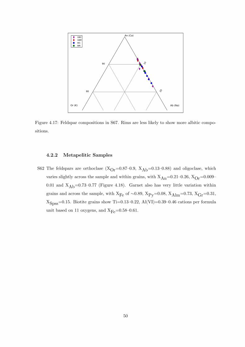
Figure 4.18: Graph to show distribution of feldspar compositions in S62.
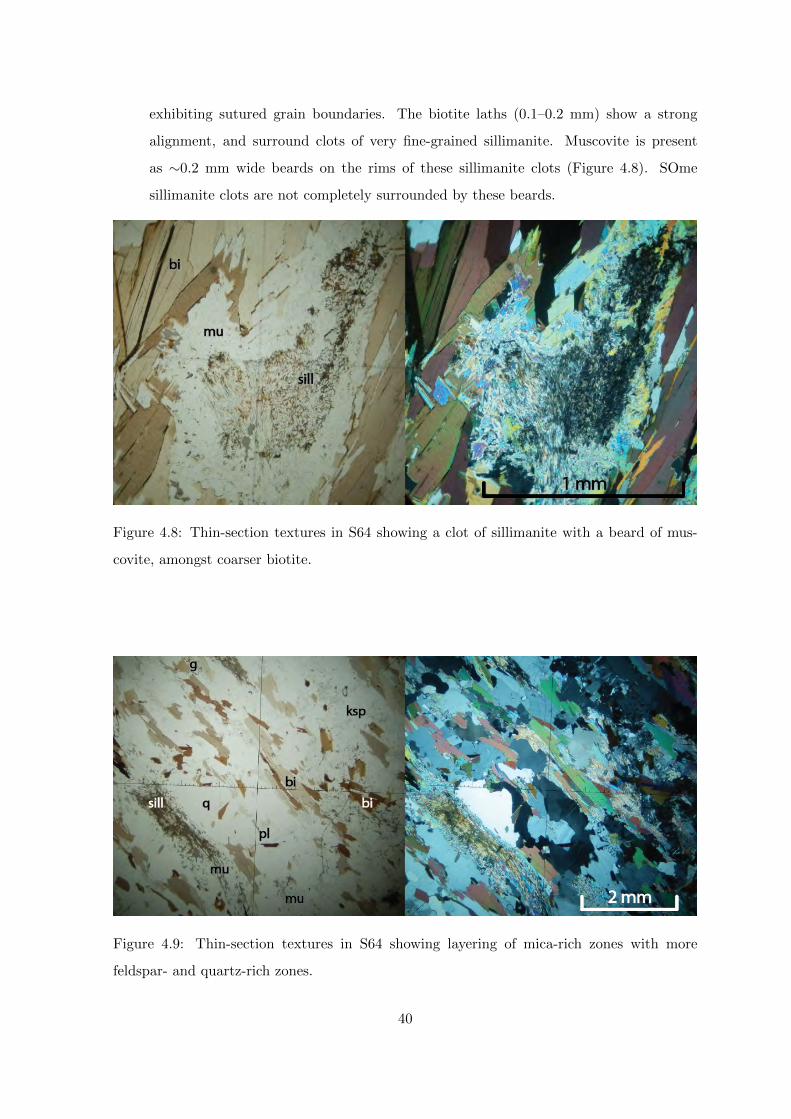
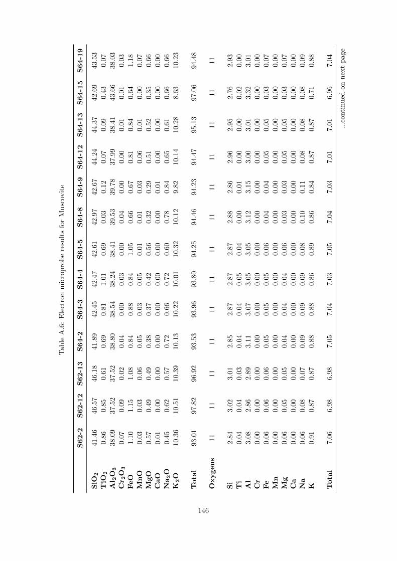
S64 The feldspars are orthoclase (XOr∼0.90, XAb∼0.10) and oligoclase, which shows XAn=0.19–
0.25, XOr=0–0.2 and XAb=0.71–0.80 (Figure 4.19). Garnet compositions are quite
uniform across the sample, with XFe of ∼0.86, XPy=0.11, XAlm=0.75, XGr=0.04,
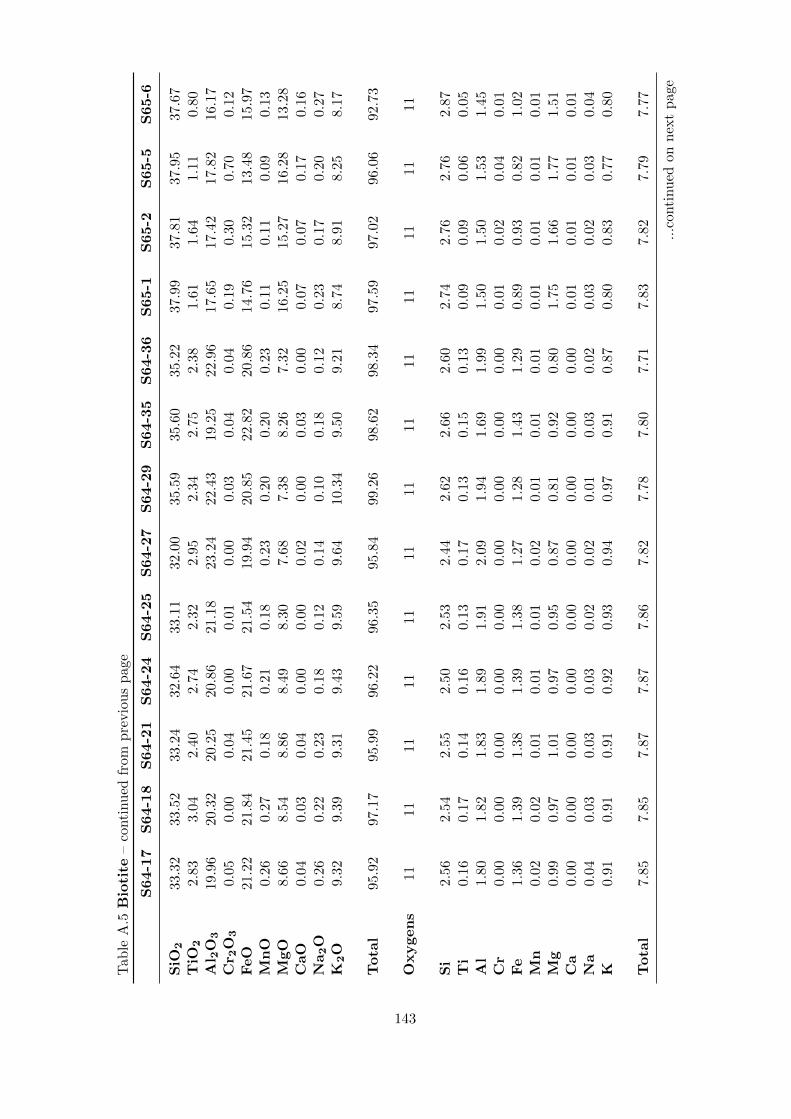
XSpss=0.10. Biotite cores show Ti=0.31–0.39, Al(VI)=0.58–0.59 cations per formula
unit based on 11 oxygens, and rims show Ti=0.36–0.53, Al(VI)=0.58–0.60.
Figure 4.19: Graph to show distribution of feldspar compositions in S64.
52
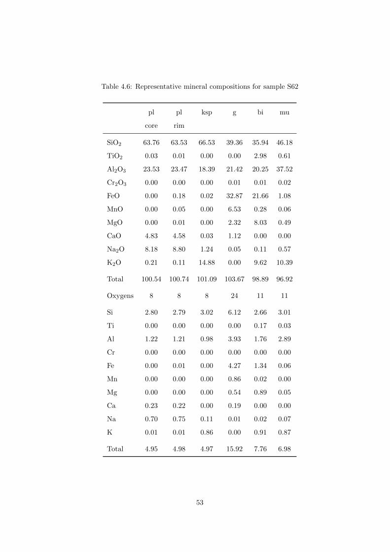
Table 4.6: Representative mineral compositions for sample S62
pl pl ksp g bi mu
core rim
SiO2 63.76 63.53 66.53 39.36 35.94 46.18
TiO2 0.03 0.01 0.00 0.00 2.98 0.61
Al2O3 23.53 23.47 18.39 21.42 20.25 37.52
Cr2O3 0.00 0.00 0.00 0.01 0.01 0.02
FeO 0.00 0.18 0.02 32.87 21.66 1.08
MnO 0.00 0.05 0.00 6.53 0.28 0.06
MgO 0.00 0.01 0.00 2.32 8.03 0.49
CaO 4.83 4.58 0.03 1.12 0.00 0.00
Na2O 8.18 8.80 1.24 0.05 0.11 0.57
K2O 0.21 0.11 14.88 0.00 9.62 10.39
Total 100.54 100.74 101.09 103.67 98.89 96.92
Oxygens 8 8 8 24 11 11
Si 2.80 2.79 3.02 6.12 2.66 3.01
Ti 0.00 0.00 0.00 0.00 0.17 0.03
Al 1.22 1.21 0.98 3.93 1.76 2.89
Cr 0.00 0.00 0.00 0.00 0.00 0.00
Fe 0.00 0.01 0.00 4.27 1.34 0.06
Mn 0.00 0.00 0.00 0.86 0.02 0.00
Mg 0.00 0.00 0.00 0.54 0.89 0.05
Ca 0.23 0.22 0.00 0.19 0.00 0.00
Na 0.70 0.75 0.11 0.01 0.02 0.07
K 0.01 0.01 0.86 0.00 0.91 0.87
Total 4.95 4.98 4.97 15.92 7.76 6.98
53
Table 4.7: Representative mineral compositions for sample S64
pl pl ksp g bi mu sill
core rim
SiO2 58.59 59.48 43.01 36.92 32.69 42.61 33.66
TiO2 0.02 0.00 0.06 0.04 2.73 0.69 0.04
Al2O3 23.60 24.31 37.37 22.05 20.51 38.41 66.41
Cr2O3 0.00 0.00 0.00 0.04 0.03 0.00 0.04
FeO 0.00 0.16 0.79 34.58 21.16 1.05 0.16
MnO 0.03 0.02 0.02 4.21 0.19 0.01 0.06
MgO 0.02 0.00 0.37 2.90 8.54 0.56 0.01
CaO 4.55 4.78 0.00 1.85 0.01 0.00 0.02
Na2O 8.43 8.68 0.71 0.01 0.20 0.60 0.04
K2O 0.35 0.10 9.63 0.00 9.35 10.32 0.05
Total 95.59 97.53 91.96 102.59 95.42 94.25 100.47
Oxygens 8 8 8 24 11 11 11
Si 2.72 2.71 2.15 5.84 2.52 2.87 2.00
Ti 0.00 0.00 0.00 0.00 0.16 0.04 0.00
Al 1.29 1.30 2.20 4.11 1.87 3.05 4.65
Cr 0.00 0.00 0.00 0.00 0.00 0.00 0.00
Fe 0.00 0.01 0.03 4.57 1.37 0.06 0.01
Mn 0.00 0.00 0.00 0.56 0.01 0.00 0.00
Mg 0.00 0.00 0.03 0.68 0.98 0.06 0.00
Ca 0.23 0.23 0.00 0.31 0.00 0.00 0.00
Na 0.76 0.77 0.07 0.00 0.03 0.08 0.00
K 0.02 0.01 0.61 0.00 0.92 0.89 0.00
Total 5.02 5.03 5.09 16.10 7.86 7.05 6.68
54
4.3 Inferred equilibrium assemblages
4.3.1 Mafic Samples
All mafic samples are amphibolites. Some exhibit traces of a higher-grade history in the form
of garnet-breakdown textures, and some show extensive retrogression and replacement of peak
minerals, (such as muscovite replacing sillimanite and K-feldspar) commonly in texturally
isolated areas.
S33 shows one textural assemblage comprising diopside, hornblende, plagioclase, sphene
and quartz. The edges of hornblende grains show lower Na and Al(VI) values than the rims,
particularly where these grains are in contact with clinopyroxene grains, where Al(VI) is
generally less than 0.2 cations per formula unit (based on 23 oxygens). This indicates that
hornblende was partially re-equilibrated towards an actinolitic composition, with grains in
contact with clinopyroxene showing more extensive retrogression. Thus it is assumed that
apart from the altered rims of hornblende grains and the actinolite on the rims of clinopyrox-
ene, the minerals and mineral compositions represent an equilibrium assemblage. Therefore
the inferred peak assemblage is diopside, hornblende, plagioclase, sphene and quartz, with
inferred retrograde alteration to form actinolite on the rims of clinopyroxene grains.
In S53, there is no significant zoning of the amphibole grains and there are no separate
textural domains in the thin section. Grain compositions are fairly consistent across the
sample and the majority of grains show annealed boundaries, indicating all minerals are
in equilibrium, resulting in an inferred peak assemblage of hornblende, biotite, plagioclase,
sphene and quartz.
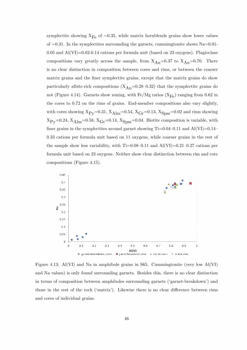
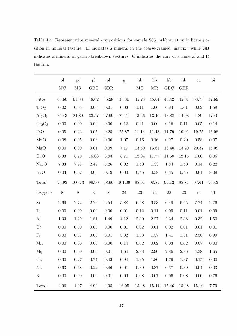
S65 and S67 both show two distinct textural assemblages. In S65, the first assemblage
is made up of coarse euhedral grains of biotite, hornblende, plagioclase and inferred garnet.
The second assemblage is confined to symplectites that pseudomorph garnets. It consists of
biotite, hornblende, plagioclase and cummingtonite, intergrown around resorbed garnets. The
first assemblage (with the addition of garnet) is interpreted as representing an equilibrated
matrix of minerals, in which the second assemblage formed owing to the breakdown of coarse
garnet grains. While there is little compositional difference between the hornblende in the
different assemblages, the plagioclase in the peak assemblage shows compositions of XAn∼0.3
that are not seen in the grains of the garnet-breakdown assemblage. Biotite grains in the this
assemblage show a wider range of Ti and Al(VI) content than grains in the peak assemblage.
In S67, the inferred peak assemblage is characterised by coarse euhedral grains of horn-
55
blende and biotite that show a strong alignment, inferred coarse garnets, and interstitial
grains of plagioclase. The secondary assemblage is characterised by finer anhedral grains
of hornblende and biotite, that do not show alignment and are intergrown with plagioclase
around resorbed garnet grains. While there does not seem to be any significant composi-
tional difference between the plagioclase or biotite grains in the two assemblages, hornblende
in the first assemblage shows higher Na and Al(VI) values than in the second assemblage.The
second assemblage is inferred to have formed as a result of the breakdown of coarse garnet
grains in the first assemblage and is therefore considered to be retrograde and, due to a lack
of mineral alignment, to have formed after the fabric-forming deformation.
4.3.2 Metapelitic Samples
Both S62 and S64 show evidence of having been granulites, containing in-situ leucosome in
outcrop. Thus, the muscovite in the sample cannot have been in equilibrium with the peak
assemblage as it would have been consumed to make melt (White & Powell, 2002). In S62,
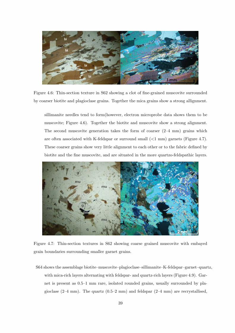
muscovite is present as either a fine mass of needle-like grains, resembling the fibrous clots
that sillimanite needles tend to form, or as medium-coarse grains with which appear to have
formed at the expense of K-feldspar. (Figures 4.6 and 4.7). In S64 the muscovite is present
as a beard on the rim of sillimanite clots (Figure 4.8). It therefore appears that all muscovite
in these samples formed through the retrograde breakdown of peak granulite facies minerals,
and so must have formed as a result of rehydration and retrogression of the samples.
S62 shows an inferred peak assemblage of biotite, garnet, K-feldspar, plagioclase quartz
and ilmenite, with the inferred presence of melt. Sillimanite may have been present, but has
been completely replaced by muscovite during retrogression and rehydration. S64 shows the
same assemblage but with sillimanite definitely present. It is inferred that melt was present
at peak conditions, but then froze following the start of retrograde metamorphism. With the
addition of fluid, muscovite then formed to completely replace sillimanite and partially replace
K-feldspar. (In S64 the replacement of sillimanite was less extensive, perhaps because less
fluid was added.) Garnet also appears to have undergone breakdown, and is only present as
small remnants, surrounded by plagioclase. The other peak minerals are still stable, making
the inferred retrograde assemblage for S62 muscovite, biotite, plagioclase, K-feldspar, quartz
and ilmenite, and for S64 the same but with sillimanite still stable.
56
Chapter 5
Mineral Equilibria Modelling
The metamorphic evolution of the Nupskapa samples was investigated through the use of cal-
culated pseudosections to determine the P–T conditions preserved by the mineral assemblages
present in the samples.
5.1 Methodology
Pseudosections were calculated in the model system Na2O–CaO–K2O–FeO–MgO–Al2O3–
SiO2–H2O–TiO2–Fe2O3 (NCKFMASHTO) using THERMOCALC 3.33 (Powell and Holland,
1988, updated June 2009) with an updated version of the internally consistent dataset of
Holland and Powell (1998, dataset file tc-ds55.txt, created 22/11/2003).
The phases considered in the modelling and references to the activity-composition models
used are biotite (White et al., 2007) , epidote (Holland & Powell, 1998), orthopyroxene
and spinel–magnetite (White et al., 2002), muscovite–paragonite (Coggon & Holland, 2002),
amphibole (Diener et al., 2007, updated by Diener & Powell, 2012), clinopyroxene (Green
et al., 2007), updated by (Diener & Powell, 2012), chlorite (Holland et al., 1998), plagioclase–
K-feldspar (Holland & Powell, 2003) and ilmenite–hematite (White et al., 2000). The sphene,
quartz and aqueous fluid (H2O) are pure end-member phases.
Bulk rock compositions for the samples were determined by X-ray fluorescence (XRF)
analysis using a Philips X’Unique II wavelength-dispersive spectrometer housed at the Uni-
versity of Cape Town. The XRF results are presented in Table 5.1. Selected analyses were
converted to the NCKFMASHTO system by disregarding the small amounts of MnO, Cr2O3
and P2O5 and converting selected amounts of total Fe to Fe3+. For the pelitic samples ∼10%,
57
and for the mafic samples ∼15%, of total Fe was converted to Fe3+ (Diener and Powell, 2010).
These re-calculated values are presented in Table 5.2.
Table 5.1: XRF whole-rock analyses of selected samples
S33 S53 S62 S64 S65 S67
SiO2 49.31 44.79 54.12 59.31 45.49 48.78
TiO2 1.05 1.32 1.27 0.88 0.91 2.76
Al2O3 14.38 14.69 19.94 18.18 14.45 14.91
Fe2O3 11.60 14.21 10.04 7.96 12.20 13.84
MnO 0.19 0.20 0.10 0.11 0.16 0.19
MgO 7.19 9.27 3.20 2.67 12.33 6.68
CaO 9.60 10.13 1.35 1.98 10.19 8.90
Na2O 3.07 2.29 2.56 2.90 1.51 0.86
K2O 1.66 1.82 5.29 4.00 0.53 1.42
P2O5 0.16 0.10 0.08 0.12 0.10 0.41
SO2 0.01 0.02 0.01 0.01 0.04 0.03
Cr2O3 0.06 0.07 0.05 0.04 0.12 0.06
NiO 0.03 0.02 0.01 0.01 0.05 0.01
H2O- 0.55 0.07 0.09 0.04 0.06 0.05
LOI 0.65 0.58 1.33 1.02 1.38 0.91
Total 99.52 99.57 99.45 99.23 99.53 99.82
The abundant leucosome present in the metapelitic samples is consistent with the rocks
having produced a significant amount of melt. However, the peak granulite facies assemblage
is well preserved, indicating that a significant amount of melt was lost from these rocks before
substantial cooling occurred (White & Powell, 2002). The petrography of the pelitic samples
suggests muscovite formed at the expense of sillimanite and K-feldspar, which is consistent
with rehydration (Spear, 1995). The current composition of these rocks therefore represents
that of a residuum that has been modified first by melt loss, and then by the addition of
fluid. For the residuum pseudosections, H2O content for each sample was estimated such
that the inferred peak assemblage was stable at conditions immediately above the residuum
solidus, to reflect conditions where the assemblage would have been in equilibrium with the
58
Table 5.2: Bulk compositions (in mol %) used to construct pseudosections
S33 S53 S62 S64 S65 S67
Si 53.31 47.98 62.53 67.21 47.83 53.34
Ti 0.86 1.07 1.11 0.75 0.72 2.27
Al 9.17 9.27 13.58 12.14 8.96 9.61
FeT 9.44 11.46 8.73 6.79 9.66 11.39
Mn 0.17 0.18 0.10 0.11 0.15 0.17
Mg 11.58 14.79 5.50 4.51 19.32 10.89
Ca 11.12 11.62 1.68 2.40 11.48 10.43
Na 3.21 2.38 2.87 3.18 1.54 0.91
K 1.15 1.24 3.90 2.89 0.36 0.99
O 0.70 0.85 0.45 0.30 0.75 0.85
remaining melt (White et al., 2004; Diener et al., 2008). For the rehydrated pseudosections,
the minimum H2O content needed to stabilise the retrograde assemblage was selected. Fluid
was assumed to be in excess for the mafic amphibolites, and no mafic granulites were selected
for pseudosection calculations because the current silicate melt model is not appropriate for
mafic compositions and their suprasolidus evolution cannot be quantitatively investigated
yet (White & Powell, 2002). Where necessary, contours were calculated for mineral compo-
sitions and in some cases, mineral modes. These were used to further constrain pressure and
temperature ranges of stable assemblages. The calculated pseudosections are presented in
Figures 5.1 to 5.8.
5.2 Results
5.2.1 Mafic Samples
S65
The inferred peak assemblage of hornblende, rutile, quartz, plagioclase and garnet (with
biotite and H2O in excess) is stable over a large P-T range, above 9 kbar and at more than
725 ◦C (Figure 5.1). The field is bounded by the breakdown of garnet below ∼9 kbar, and
of plagioclase to lower temperatures. At higher temperatures and lower pressures, quartz
59
breaks down. The peak assemblage field was contoured for Fe/Mg ratio in garnet. These
contours are sensitive to changes in pressure and temperature, and show that the Fe/Mg ratio
increases with decreasing temperature and pressure. The contours range from XFe=0.60 at
the high end of the field, to XFe=0.72 at the lower end.
500 550 600 650 700 750 800 850 900
3
4
5
6
7
8
9
10
11
12
13
14
450
act hb chlep ru q
act chl ep sph
q ab
act hbchl epsph q
act chl sph ep
q gl
hb chlep ru q
hbchl epsph q
act hbchl epsph q
pl
hb chlru q
hb chlru qpl
hb ru q hb ru q pl
hb ru pl
hb ru q g
hb ru q pl g
hb ru pl g
hb ru q pl cu
hb ru pl cu
hb epru q g
S65act glchl ep
ru qhb chlep ruq g
0.73
0.74
0.76
0.77
0.78
0.75
NCKFMASHTO (+bi+H2O)
0.60
0.61
0.620.63
0.64
0.650.66
0.670.680.690.700.710.72
Temperature (ºC)
Pres
sure
(kba
r)
Figure 5.1: Calculated pseudosection for S65. The inferred peak assemblage stability field
(hb–ru–q–pl–g) has been contoured for XFe ratio in garnet. These range from 0.60 at high
T and P, to 0.72 at lower T and P. The inferred retrograde assemblage stability field (hb–
ru–q–pl–cu) was too small to warrant contouring, but the field between the inferred peak
and retrograde fields (hb–ru–q–pl) has been contoured for anorthite content in plagioclase
(dotted lines). These show decreasing values from higher to lower pressures.
Between ∼600 and 700 ◦ , at 4-6 kbar below garnet stability, cummingtonite becomes
60
stable and quartz breaks down almost immediately thereafter. The inferred retrograde as-
semblage, present in the garnet-replacement textures, is then hornblende, rutile, quartz,
plagioclase and cummingtonite and is stable in a narrow field between 585 and 705 ◦C, and
3.3 and 6.0 kbar. However, the position of the quartz-breakdown line is highly dependent on
Si content in the rock, and so the lower pressure estimate is far less reliable than the upper
(Figure 5.1).
S67
The inferred peak assemblage of hornblende, quartz, rutile, plagioclase and garnet (with
biotite and H2O in excess) is stable above 7 kbar, and from 650 to above 850 ◦C . The
assemblage is bounded by the breakdown of garnet to lower pressures, and by the stabilisation
of epidote to lower temperatures (Figure 5.2).
Contours showing Fe/Mg ratio in garnet and anorthite content in plagioclase vary from
XFe=0.74, XAn=0.76 at 10 kbar and 800 ◦C , to XFe=0.88, XAn=0.90 at 7 kbar and 650 ◦C ,
in the stability field of the peak assemblage. The retrograde assemblage of hornblende, quartz,
rutile, plagioclase, biotite and excess H2O is stable at 550-650 ◦C and 3–7 kbar (Figure 5.2).
The field is bounded by the garnet-breakdown line to higher pressures, and the stabilisation
of epidote to lower temperatures and cummingtonite to lower pressures. Towards higher
temperatures, orthopyroxene becomes stable.
61
450 500 550 600 650 700 750 800 850
2
3
4
5
6
7
8
9
10
11
12
0.84
0.860.
88
0.9
0.8
0.82
0.84
0.860.880.9
0.74
0.76
0.78
0.80
0.82
0.84
hb q ru g ep
hb chlep qru g
hb chlep q
ru
hb chlep sph
q ru
gl chlep sph
q ru
hb q
ru g
ep
pl
hb q ru g pl
hb q ru pl
hb q ru pl cu
hb c
hl e
pab
sph
q
hb q rupl chl
hb chlep plsph q
chlact ep ab sph q
hb ch
lep
q ru
pl
hb chlep plsph q
ru
hb q ru ep pl
NCKFMASHTO (+bi+H2O)S67
hb q ru pl opx
Temperature (ºC)
Pres
sure
(kba
r)
Figure 5.2: Calculated pseudosection for S67. The inferred peak assemblage stability field
(hb–q–ru–g–pl) has been contoured for XFe ratio in garnet (dashed lines) and anorthite
content in plagioclase (solid lines). Both sets of contours have fairly shallow negative slope
and increase towards lower P and T. The inferred retrograde assemblage stability field (hb–
q–ru–pl) has also been contoured for anorthite content in plagioclase. These steeper contours
have a positive slope and increase with decreasing T.
S33
The inferred peak assemblage of diopside, hornblende, plagioclase, sphene and quartz (with
biotite and H2O in excess) is stable over a wide range of pressures, from 4 to 11 kbar, and a
narrower range of temperatures, from 525 to 700 ◦C. The field is bounded by the stabilisation
of epidote to lower temperatures and higher pressures, actinolite to lower temperatures at low
62
pressures, and of rutile to higher temperatures. To lower pressures quartz breaks down and at
higher pressures (greater than ∼11 kbar) garnet becomes stable. This field was contoured for
Na content in hornblende. The contours are sensitive to pressure, and range from XNa=0.29
at ∼4 kbar to XNa=0.55 at ∼9 kbar. The presence of actinolitic rims on hornblende grains,
and of actinolite alteration rims on clinopyroxene grains implies a retrograde assemblage of
diopside, hornblende, plagioclase, sphene, quartz and actinolite (with biotite and H2O in
excess) which is stable over a small area, from 510–520 ◦C and 3–3.4 kbar. The field is
bounded by the breakdown of quartz to lower pressures, and by the stabilisation of epidote
to higher pressures.
450 500 550 600 650 700 750 800
5
6
7
8
9
10
11
12
13
14
4
3
0.29
0.31
0.33
0.45
0.47
0.49
0.51
0.53
0.55
0.35
0.37
0.39
0.41
0.43
NCKFMASHTO (+bi+H2O)S33
di hb pl ep sph q
act gl o ep sph q
di hb pl ilm qdi hb pl sph q
di hb pl ep ru q g
act ep chl ab q
di hb ab
ep sph q
o hb ep ru q
di hb pl sph
di hb pl ilm
di hb pl ru q g
act ep chl ab
di h
b pl
sph
ru q
act hb ab ep sph q
act h
b pl e
p
sph q
act h
b pl e
p sph
act di hb pl ep sph q
hb o ep sph q
hb o ep ab sph qdi hb pl ilm q g
act gl o ep ru q
Temperature (ºC)
Pres
sure
(kba
r)
Figure 5.3: Calculated pseudosection for S33. The inferred peak assemblage stability field
has been contoured for A-site Na in hornblende, and these range from 0.55 at ∼9 kbar and
∼650 ◦C , to 0.29 at ∼3 kbar and ∼550 ◦C
63
S53
The inferred diopside-free peak metamorphic assemblage of hornblende, plagioclase, sphene,
biotite and excess fluid seen in S53 is not stable anywhere in the S53 pseudosection. However,
this assemblage with additional diopside is stable over a wide range of pressures and tempera-
tures. The field is bounded by the presence of orthopyroxene to higher temperatures, and by
garnet to higher pressures. Calculations show that the modal proportions of diopside in this
field is uniformly low, between 1 and 6 volume %. The sample does not contain any epidote
or quartz (stabilised to lower temperatures) or garnet such that the best representation of
the peak assemblage on the pseudosection is taken to be hornblende, plagioclase, sphene,
biotite and diopside with possible fluid. The discrepancy between the sample and the model
could be the result of the bulk composition not accurately representing the thin section or
the presence of diopside being easily overlooked owing to its low abundance. This field is
stable over a wide range of temperatures, above 475 ◦C and below 10 kbar (Figure 5.4). The
diopside-bearing peak field has also been contoured for anorthite content in plagioclase (solid
lines). These contours have a positive slope and increase towards higher temperature and
lower pressure conditions.
64
450 500 550 600 650 700 750 800 850
2
3
4
5
6
7
8
9
10
hb di pl sph
act hb ep ab
sph chl
hb di pl sph opx
hb di pl sph g
hb di pl sph q ep
hb di pl sph q
act hb ep sph
chl
hb pl sphq ep
hb d
i pl s
ph e
p
hb p
l sph
ep
act
hb p
l sph
ep
act c
hl
hb p
l sph
ep
hb absphq ep
NCKFMASHTO (+bi+H2O)S53
0.47
0.48
0.49
0.50
0.01
0.02
0.03
0.04
0.05
0.06
Temperature (ºC)
Pres
sure
(kba
r)
Figure 5.4: Calculated pseudosection for S53. The inferred peak assemblage stability field has
been contoured for the mode of diopside in the sample (dotted lines), which range from 1 vol.
% at lower pressures and temperatures, to 6 vol. % at higher temperatures and pressures.
The field has also been contoured for anorthite content in plagioclase (solid lines). These
contours have a positive slope and increase towards higher temperature and lower pressure
conditions.
5.2.2 Metapelitic Samples
S62
The inferred granulite facies peak assemblage of biotite, garnet, K-feldspar, plagioclase,
quartz, sillimanite, ilmenite and melt is stable on the residual pseudosection between 820
and 880 ◦C , and 6.4–11.6 kbar (Figure 5.5). The field is bounded by the solidus to lower
temperatures and by biotite breakdown to higher temperatures. To higher pressures, kyanite
65
is stable instead of sillimanite, and cordierite becomes stable at pressures below ∼6 kbar.
The inferred retrograde assemblage of muscovite, biotite, plagioclase, K-feldspar, quartz and
ilmenite is not stable anywhere on the pseudosection for the residual composition, as mus-
covite is missing. Petrographic analysis suggests that muscovite formed at the expense of
sillimanite and K-feldspar, which is consistent with rehydration (Spear, 1995). Rehydrated
pseudosections were calculated with varying fluid contents. The inferred retrograde assem-
blage becomes stable with a minimum water content of 7.5 wt% H2O, between 430 and
600 ◦C and below 5 kbar (Figure 5.6). The field is bounded by k-feldspar breakdown and the
solidus to higher temperature, and aluminosilicate stabilisation to lower temperatures and
higher pressures.
350 400 450 500 550 600 650 700 750 800 850 900
1
2
3
4
5
6
7
8
9
10
11
12
13
14 S62 residuum H2O=2% NCKFMASHTO(+ilm)
bi g ksp pl q ky
bi g ksp pl q sill
bi g ksppl q ky liq
bi g ksppl q sill
liq
bi g ksp pl q sill cd
bi g ksp pl q cdbi g ksp pl
q ky cd
bi g ksp pl q cd
liq
bi g ksp pl cd
liq
Temperature (ºC)
Pres
sure
(kba
r)
Figure 5.5: Calculated pseudosection for the residuum composition of sample S62. The
solidus is indicated with a dashed line.
66
350 400 450 500 550 600 650 700 750 800 850 900
2
3
4
5
6
7
8
9
10
11
750
mu bi pl ky ksp
mu bi pl ky
mu bi pl ksp
mu bi pl
mu
bi p
lliq
ksp
bi pl liq ksp sill
bi pl li
q ksp ky
mu bi pl si
ll
S62 rehydrate with H2O=7.25% NCKFMASHTO (+ilm+q)
Temperature (ºC)
Pres
sure
(kba
r)
Figure 5.6: Calculated pseudosection for the composition of sample S62, rehydrated with
7.25 wt% H2O. The solidus is indicated with a dashed line.
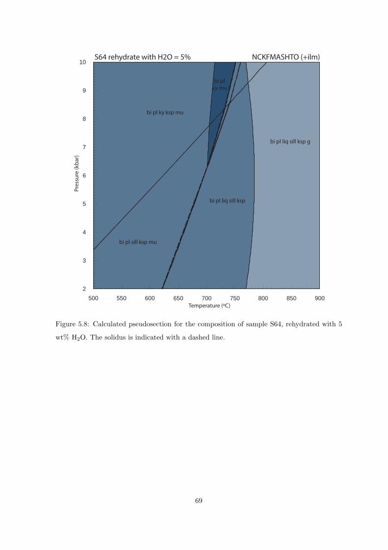
S64
The inferred granulite facies peak assemblage of biotite, garnet, K-feldspar, plagioclase,
quartz, sillimanite, ilmenite and melt is stable on the residual pseudosection between 805
and 880 ◦C , and 6.2 to 11.6 kbar (Figure 5.7). The field is bounded by biotite breakdown
to higher temperatures, and the solidus to lower temperatures. To higher pressures kyanite
replaces sillimanite, and to lower pressures cordierite becomes stable. The inferred retrograde
assemblage of muscovite, biotite, plagioclase, k-feldspar, quartz, sillimanite and ilmenite is not
stable anywhere on the pseudosection for the residual composition. Muscovite has formed on
the rims of sillimanite clots, suggesting it formed as a result of sillimanite breakdown, consis-
67
tent with rehydration (Spear, 1995). On a partially rehydrated pseudosection, calculated with
5 wt% H2O, this retrograde assemblage is stable below 700 ◦C and 7.8 kbar (Figure 5.8). The
field is bounded by the kyanite-sillimanite transition to higher pressures and by k-feldspar
breakdown, as well as melt-formation, to higher temperatures. The pressure-temperature
range constrained by this field is wide and as there is little variation in mineral composition
across the sample, contours are of little use in constraining it further.
650 700 750 800 850
2
3
4
5
6
7
8
9
10
1
4
bi g ksp pl sill
bi g ksp pl cd
bi g ksp pl sill liq
bi g ksp pl sill cd
bi g ksp pl cd liq
g ksp pl cd liq opx
bi g ksp pl cd opx
bi ksp pl cd opx
ksp pl cd liq opx
g ks
p pl
cd
liq
bi g ksp pl ky
S64 residual NCKFMASHTO (+q+ilm)
Temperature (ºC)
Pres
sure
(kba
r)
Figure 5.7: Calculated pseudosection for the residuum composition of sample S64. The
solidus is indicated with a dashed line.
68
650 700 750 800 850 900
2
3
4
5
6
7
8
9
10
550 600500Temperature (ºC)
Pres
sure
(kba
r)
S64 rehydrate with H2O = 5% NCKFMASHTO (+ilm)
bi pl ky ksp mu
bi pl sill ksp mu
bi pl liq sill ksp
bi pl liq sill ksp g
bi plky mu
Figure 5.8: Calculated pseudosection for the composition of sample S64, rehydrated with 5
wt% H2O. The solidus is indicated with a dashed line.
69
Chapter 6
Discussion
6.1 Estimation of peak and retrograde P-T conditions
6.1.1 Mafic Samples
In sample S65, Fe/Mg ratios in garnet show that garnet grains are commonly zoned, with cores
showing XFe=0.62 and rims showing XFe=0.72. Contours in the peak assemblage stability
field show an increase in XFe in garnet with a decrease in pressure and temperature. This
indicates that the sample underwent re-equilibration following decompression from more than
14 kbar to below 9 kbar where garnet was no longer stable (Figure 5.1). The replacement of
garnet by plagioclase and cummingtonite indicates further decompression to around 5 kbar,
at ∼640 ◦C , where the retrograde assemblage developed.
Sample S67 shows zoning in both the plagioclase and garnet grains. Contouring the peak
assemblage field for anorthite content in plagioclase and Fe/Mg ratio in garnet shows that
plagioclase becomes more anorthitic, and garnet more Fe-rich, with a decrease in pressure
and, to a lesser extent, temperature. The increase from core to rim in anorthite content in
plagioclase and Fe content in garnet shows the sample experienced retrogression followed by
garnet breakdown, from above ∼10 kbar and ∼800 ◦C to conditions at the lower-temperature
end of the hb-q-ru-pl (+bi+H2O) stability field (Figure 5.2). Plagioclase rims show XAn=0.9,
and therefore the retrograde assemblage can be constrained to 550–665 ◦C and 3–6.8 kbar.
The fabric in S67, defined by the alignment of biotite, hornblende and ilmenite, anasto-
moses around the garnet relics, which appear unaffected by the deformation, as the plagioclase-
cummingtonite-biotite symplectite displays the sub-idioblastic shape of the original garnet.
The biotite within the breakdown-textures is not aligned, whereas the biotite in the rest of the
70
sample is strongly aligned. This indicates that garnet breakdown (and therefore retrograde
metamorphism) must have occurred after the main fabric-forming deformation event.
Sample S33’s stability field is confined to a narrow range of temperatures, from 520 to
700 ◦C , but a very wide range of pressures. It overlaps with S67 and S53 between 550 and
650 ◦C , and from 3 to 6.4 kbar (Figure 5.3). Contouring the field for Na in hornblende
indicates a decrease in Na content with a decrease in pressure (Figure 5.3). Zoning in horn-
blende grains in S33 shows the cores to be more Na- and Al-rich than the rims (Figure 4.10),
indicating a decompressive retrogression. Exactly how much cooling occurred during this
retrogression is unconstrained, but it was likely more than ∼150 ◦C . S33 does not preserve
evidence of a separate peak assemblage, but the zoning preserved in the hornblende shows
clear evidence of decompression, with some potential cooling.
The stable assemblage in S53 is less tightly constrained than the other samples as the
assemblage is stable over a very wide field. This field overlaps with the conditions constrained
by S33, S65 and S67. Microprobe data shows the cores of plagioclase grains as less anorthitic
than the rims (XAncore=0.30, XAnrim=0.48). As XAn increases across the field, with de-
creasing pressure and increasing temperature, the zoning could be the result of decompression
with minimal temperature changes (Figure 5.4).
6.1.2 Summary of metamorphic conditions recorded by mafic samples
Both S65 and S67 show clear evidence for a peak assemblage followed by decompression and
cooling to form a retrograde assemblage. If the peak assemblage fields for S65 and S67 are
overlapped, they constrain a range of peak metamorphic conditions above 735 ◦C at more
than 9 kbar (Figure 6.1).
Overlapping the retrograde assemblage fields of all four samples shows that S33, S53 and
S67 all overlap and constrain a pressure and temperature field between 555 and 645 ◦C , and
3.2 and 6.4 kbar (Figure 6.1). The retrograde assemblage in S65 sits at slightly lower pressures
and higher temperatures, and this may be because the retrograde assemblage developed in
isolated pockets, out of equilibrium with the rest of the rock, and so this assemblage was
modelled with the incorrect/inappropriate bulk composition.
The zoning in S65 and S67 (where plagioclase cores are more anorthitic than rims, and
garnet cores are more Fe-rich than rims) indicates retrograde re-equilibration of some kind.
This could show early retrogression after peak conditions, from above ∼800 ◦C at 10 kbar,
71
to ∼720 ◦C at 8 kbar (Figures 5.1 and 5.2). However, the zoning in these minerals may
also simply represent the partial re-equilibration of the peak assemblage to the retrograde
conditions at a later stage. The zoning is not used in constraining the P-T conditions, but
does indicate the trajectory of retrogression at some point in the poly-metamorphic history.
6.1.3 Summary of conditions recorded by metapelitic samples
Samples S62 and S64 overlap to constrain peak temperatures and pressures to be essentially
those constrained by S62. The upper P limit of the peak stability field in both samples is the
kyanite-sillimanite transition. It is therefore possible that the samples experienced conditions
where kyanite was stable, but that during decompression this kyanite broke down to form
sillimanite. Thus the samples may have come from higher pressures than those recorded
here (perhaps similar to the conditions suggested by Board et al. (2005)). The sillimanite
in S64 is clearly replaced, at least partially, by muscovite. It is likely that the same process
occurred in S62, but to a greater extent, resulting in the complete replacement of sillimanite by
muscovite. Together, the peak fields of S62 and S64 constrain peak metamorphic conditions
to be between 820 and 880 ◦C , and 6.4–11.6 kbar. The retrograde assemblages of S62 and
S64 overlap between 500 and 605 ◦C at less than 5 kbar (Figure 6.1).
6.2 Likely P-T paths and comparisons with previous work
Overlapping the conditions constrained by the pelitic samples with those constrained by the
mafic samples shows that the peak conditions overlap between 820 and 880 ◦C , at 9.5–11.6
kbar, while the retrograde conditions show overlap between 555 and 595 ◦C , at 3.2–4.8 kbar.
It may be that both the peak and retrograde conditions recorded in the Nupskapa area oc-
curred during the Pan-African event, such that a direct transition occurred, from ∼850 ◦C at
12.5 kbar, to ∼575 ◦C at 4 kbar (Figure 6.2). However, based on previous metamorphic
studies conducted in the area (e.g. Groenewald & Hunter, 1991; Groenewald et al., 1995;
Grantham et al., 1995; Board et al., 2005), the ‘peak’ conditions are instead closer to the M1
conditions of Groenewald & Hunter (1991), indicating a likely Grenvillian age for this assem-
blage (see Figure 6.4). The ‘retrograde’ conditions are recorded by minerals that formed after
the fabric-forming deformational event. This event was dated by Board (2001) and found to
have an age of ∼ 540 Ma, indicating that the post-tectonic ‘retrograde’ conditions are likely
have occurred during a late stage of the M2 metamorphic event. These M2 conditions are
72
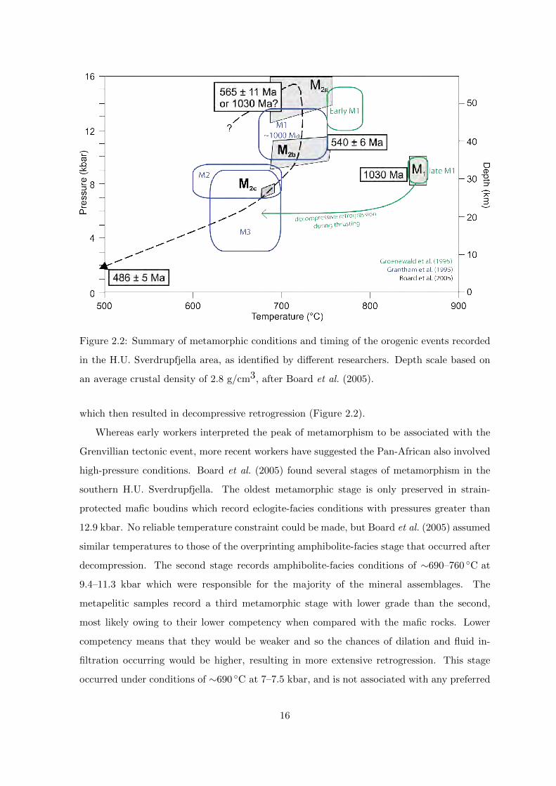
Figure 6.1: Overlapping the stable assemblage fields for all 6 samples shows that the mafic
samples overlap to constrain peak conditions above 735 ◦C at more than 9 kbar, and retro-
grade conditions of 555–645 ◦C , and 3.2–6.4 kbar. The pelitic samples overlap to constrain
peak conditions of 820–880 ◦C , at 6.4–11.6 kbar. The retrograde assemblages of S62 and S64
overlap between 500 and 605 ◦C at less than 5 kbar. Final constrained conditions are shaded
in yellow, and show that peak conditions were between 820 and 880 ◦C at 9.5–11.6 kbar, while
the retrograde conditions were between 555 and 595 ◦C at 3.2–4.8 kbar.
lower than the three sets of M2 conditions identified by Board et al. (2005). However, they
do lie along the retrograde path, between the M2c stage and the point at which the rocks
reached the ∼500 ◦C closure temperature of hornblende (at ∼486 Ma; Figure 6.4). Thus it
appears plausible that the ‘peak’ and ‘retrograde’ conditions of this study are likely to have
resulted from two separate metamorphic cycles, and that there is evidence of both Grenvillian
and Pan-African metamorphism recorded in the Nupskapa area (Figure 6.3). A more certain
P-T-t path for the Nupskapa area could be achieved through isotopic dating of the minerals
that make up the different assemblages but that is beyond the scope of this study.
73
Figure 6.2: P-T path if both conditions occurred during the Pan-African orogeny.
Figure 6.3: Possible P-T paths if the peak conditions occurred during the Grenvillian orogeny,
and the retrograde conditions during the Pan-African orogeny.
74
Both Groenewald et al. (1995) and Board et al. (2005) found evidence for eclogite-facies
metamorphic conditions, around 750 ◦C at more than 12 kbar. Groenewald et al. (1995)
attributed these to an early M1 event while Board et al. (2005) related them the M2a Pan-
African event (Figure 6.4). No evidence was found in the Nupskapa area for similar high-
pressure conditions. The samples collected in the Nupksapa area record much higher tem-
peratures than those of the M2a event (Figure 6.4). The stability field of S33 is situated at
the right temperatures for the M2a event, and is bounded by the garnet breakdown line to
higher pressures. If garnet relics were found in this sample one could infer that S33 might
potentially have experienced conditions similar to the M2a conditions of Board et al. (2005).
However, none were found in either the hand sample or thin section. The high-pressure con-
ditions identified by Board et al. (2005) were for an inferred assemblage, based on Na content
in clinopyroxene, which suggested it was originally omphacite. The clinopyroxene in samples
from the Nupskapa area have very low sodium and aluminium content (Table 4.2), and so no
high-pressure omphacite-bearing assemblage was inferred for this study.
Figure 6.4: The peak and retrograde conditions recorded in the Nupskapa area (red), com-
pared with the P-T conditions identified by Groenewald et al. (1995) (green), Grantham et al.
(1995) (blue) and Board et al. (2005) (black with grey shading).
75
Regardless of the details of the early poly-metamorphic history of the Nupskapa area, the
late-M2 conditions are recorded in a post-tectonic assemblage, made up of minerals that do
not show any preferred orientation. The retrogression associated with the formation of this
assemblage required the introduction of fluid into the crust (White & Powell, 2002). The
formation of the M2 shear zones is likely to have resulted in the introduction of fluid into the
host rocks, which later resulted in the formation of the retrograde assemblage. The intrusion
of the composite leucogranites occurred after the formation of these shear zones(see Fig-
ure 3.8). The late-M2 conditions are therefore likely to be the maximum physical conditions
under which intrusion of the composite dyke phase could have occurred. These conditions, of
∼575 ◦C at 4 kbar, lie between the wet solidus (Figures 5.5 to 5.8) (Vigneresse, 2006) and the
brittle-viscous transition (Handy et al., 2001), and indicate a location in the mid-crust where
temperatures are high, but more than 100 ◦C below the solidus, where a pervasive network of
small-scale melt-bearing structures would no longer be feasible, but where temperatures are
still high enough to also hinder focused migration (Weinberg, 1999; Faber, 2012). Thus, these
conditions represent a likely location where one might expect the transition from pervasive
to focused migration to occur.
6.3 Inferred style of melt migration
The P-T estimates indicate that suprasolidus conditions were reached by both metapelitic
samples, and that melting is therefore most likely to have occurred under M1 conditions.
The host-rock paragneiss of the Nupskapa Cliff should therefore contain evidence of melting
and melt segregation. The oldest intrusive phase in the cliff has a leucogranitic composition
and forms a small to mesoscale pervasive leucosome network, consisting of predominantly
centimetre-scale subhorizontal structures, with smaller diffuse stromatic leucosome structures
connecting to larger, discordant structures. The leucosomes have diffuse feathery boundaries,
and therefore appear to have been fed by melt from within the country rock (Sawyer et al.,
2011; Brown, 2013). They also exhibit pinch-and-swell and boudinage structures, and are
generally oriented parallel to the gneissic host rock fabric. The larger structures of the oldest
leucosome, although somewhat discordant to the gneissic fabric, are connected to foliation-
parallel leucosomes and connect the dilatant sites formed in the fold hinges of the foliation,
and so are still occupying pre-existing zones of weakness and low-pressure (Figure 3.3; Vernon
& Paterson, 2001). Thus this phase seems to represent melting and melt segregation within
76
the host rock during M1 granulite facies peak metamorphism.
The temperatures experienced by the Nupskapa area during M2, inferred to represent the
Pan-African event, are below the original peak conditions reached during the M1 event (even
if we take the conditions of Grantham et al. (1995); Groenewald et al. (1995) and Board
et al. (2005) as peak). The rocks would have become dehydrated during the first high-grade
metamorphic cycle and the solidus temperatures would have been elevated. Furthermore
there is no evidence that these rocks were rehydrated following M1 (which may have allowed
melting during M2, so melting is unlikely to have occurred again at the lower temperatures
of M2 peak metamorphism (White & Powell, 2002; Diener et al., 2008). Thus, even though
they reached reasonably high temperatures, the rocks exposed in the Nupskapa area do not
appear to have melted during the Pan-African M2 event. According to McGibbon (2014),
the deformation related to the Pan-African orogenic event did not form a penetrative fabric
across the Nupskapa area, but was instead partitioned into areas that were weaker due to
features such as pre-existing fabrics, finer grain sizes, retrogressed minerals and the presence
of melt. This resulted in the narrow and localised shear zones seen across the field area. The
Nupskapa cliff is not located in such a shear zone and so only represents M1 fabric formation.
Cooling and exhumation following peak M1 conditions may have involved melt fluxing
through these rocks, from anatectic rocks at greater depth. The second-oldest melt phase
(mapped in pink in Figure 3.3) shows sharp boundaries, some interconnectivity, and is less
extensive over the outcrop than the older phase. The individual structures are generally
discordant and some are at ∼90 ◦C to each other. This phase is clearly not fed by smaller
leucosomes from within the host rock, and so represents melt intrusion after the period of
initial in situ melting and melt segregation, and may be the result of melt produced at
greater depths attempting to rise through these rocks. This phase is contained in relatively
fine structures that form a pervasive network and so must have intruded when the rocks
were close to, but likely below, the solidus. The narrow structures are not deformed in the
Nupskapa outcrop, but as this phase is not that extensive across the field area it is difficult
to tell its cross-cutting relationship with the Pan-African shear zones. Thus this phase may
represent either a post-peak M1, or near-peak M2 intrusion of melt into hot, but subsolidus,
rocks.
The composite dykes form the third intrusive phase in the Nupskapa outcrop. Through
U-Pb SHRIMP dating of zircon, Board (2001) identified a late Pan-African age for these
‘monzogranitic dykes’. These dykes are sub-vertical and highly discordant to the subhor-
77
izontal gneissic fabric in the host rocks. As they cross-cut shear zones (Figure 3.8), they
must have intruded after the Pan-African thrusting event which confirms the post-tectonic
age given to these dykes by Board et al. (2005). Older leucosome structures can be matched
up across the width of individual dykes and show almost no shear displacement (maximum
∼30 cm), indicating that the dykes resulted from tensile fracture (Figure 2.4). This suggests
that their intrusion occurred during extensional or strike-slip deformation, under conditions
of low differential stress, probably coupled to high magma pressure. In the Nupskapa area,
the post-M2 mineral assemblage records conditions of ∼575 ◦C at 4 kbar. The retrograde
minerals represent late M2 conditions, after the formation of the Pan-African shear zones
(for more one the distribution of retrogression, see Sebetlela (2013)). The composite dykes
are thought to have a similar age of intrusion and so these conditions are inferred to be
the maximum physical conditions at which the dykes intruded. Based on an average crustal
density of 2.8 g/cm3, the metamorphic conditions of the country rock indicate a mid-crustal
position, at a depth of ∼15 km, when the composite dykes intruded (Figure 6.4; Board et al.,
2005).
These dykes contain several phases of leucogranite with different mineralogies and tex-
tures. The different phases do not show consistent age relations, indicating the heterogeneity
cannot be the result of successive melt batches pulsing through the same structures (a method
suggested by Brown & Solar (1998a), Bons et al. (2004) and Brown (2013), amongst others).
This implies that the source was extremely heterogeneous, and that the dykes were fed by
compositionally different melt sources simultaneously. At the least, it implies that successive
melt batches must have intruded before the previous batches had solidified or completely left
the structure.
The composite dykes range between 0.5 and 2 m in width. At the base of the cliff, narrower
dykes can be seen to coalesce and feed into the wider dykes (see Figures 3.3 and 3.7). This
same process must have occurred several times before, below the level of this outcrop, in order
for contrasting melt phases to be contained in the same structure in such a disorganised way.
It must be noted that the preserved widths of the intrusive features in the Nupskapa Cliff
are not necessarily the same as the width during melt transport through them, as large
melt-bearing structures can lose melt and appear very thin (Clemens & Mawer, 1992; Brown,
1994; Bons et al., 2004). It is also very hard to tell just how extensive these dykes were in
strike direction at the time of melt flux. While it can be estimated from generalised aspect
ratios (breadth-width-height, see Vermilye & Scholz (1995)), in the 2-dimensional outcrop
78
of the Nupskapa cliff we can only measure the width (measured perpendicular to fracture
wall) at the time of freezing. An assumption made in this study is that relative widths
are preserved, such that the smaller dykes feeding into the larger ones showed similar size
relationships during melt transport. Individual dykes show a similar lack of consistent age
relations between the different leucogranite phases. Furthermore, where two dykes join up to
make one, there does appear to be some mixing of the magmas from different sources. Thus
it is assumed that together they represent a ‘snapshot’ in time, and that the majority of the
dykes intruded near-simultaneously, rather than as separate events spread out over time.
The composite dykes show sharp, straight boundaries indicating that they formed as a
result of melt intrusion rather than melt segregation from within this outcrop. They are
mostly vertical, irrespective of the anastomosing sub-horizontal host rock fabric, and formed
through tensile fracture with negligible vertical displacement of the host rock, implying that
their intrusion was independent of existing anisotropies and occurred under low differential
stress. They show little interconnectivity, at least in the view displayed by the Nupskapa
Cliff, and are fed by smaller dykes at the base of the cliff. Therefore they do not represent a
network of in situ melt, but rather the far-field transport of melt from a spatially removed
source, anywhere from 5 to 15 km below this outcrop (Board, 2001). These features are
characteristic of a focused migration style.
The composite dykes are found right across the field area, and even beyond it in the more
eastern parts of H.U. Sverdrupfjella (Board, 2001). The numerous dykes are commonly not
more than a few metres apart. Thus, although individually they are discrete and focused
structures, together they do not represent a wholly focused melt transfer system. Further-
more, based on P-T estimates, the dykes appear to have intruded into a mid-crustal location,
and therefore into a likely position where the transition from pervasive to focused migration
can be expected to occur.
The numerical model produced by Bons et al. (2004) describes a way in which melt
migration may become more focused through a gradual coarsening of the melt network. In this
model melt moves from the grain boundaries where it is first formed into discrete batches that
make up veins. These veins grow larger as they are fed by more melt. Eventually neighbouring
veins may coalesce to make larger melt batches. As the melt volume increases, buoyancy forces
become greater and melt begins to move upward along steep veins. Eventually veins are large
enough to move through the crust without freezing and leave the system as dykes. In this
model, mixing and mingling of magmas occurs throughout the hierarchical accumulation and
79
ascent system, as smaller batches gradually join up to make larger ones (Bons et al., 2004).
This could be seen as a hybrid version of the two end-members of mixing and mingling
outlined by Collins et al. (2000), i.e. mixing and mingling does not take place solely in
the source or in the final emplacement structure but rather throughout the process of melt
migration.
Similarly, the numerical modelling of dykes in low-viscosity asthenosphere below mid-
ocean ridges, performed by Ito & Martel (2002), showed that neighbouring dykes create
distortions in the local stress field that can be attractive or repulsive according to vertical
and horizontal spacing. Two adjacent dykes will tend to merge if they initiate within a few
hundred metres of each other. This implies that smaller dykes, transporting separate melt
batches parallel to each other, could gradually begin to interact and join up, combining the
volume of melt and enabling the larger dyke to migrate further (Ito & Martel, 2002; Brown,
2013). This would result in a gradual ‘coarsening’ of the melt network, with smaller melt
structures feeding into fewer, larger ones (see Figure 1.1).
The study performed by Ito & Martel (2002) did not address the potential for interaction
of dykes in the continental crust. However, at the base of the Nupskapa cliff (and higher
up on the western side of the cliff) narrow dykes can be seen to coalesce and form wider
ones (Figure 3.7). If we assume that the relative widths along the length of the dykes were
preserved, this coalescing might be an example of the melt-focusing mechanism described by
the models of Bons et al. (2004) and Ito & Martel (2002). The vertical length of a dyke is
dependent on the aperture (width perpendicular to fracture wall) and wider dykes containing
more melt will be able to propagate further (Weertman, 1971; Clemens & Mawer, 1992).
Dykes containing more melt also contain more heat and so would be able to intrude cooler
country rock without freezing.
This model of gradual focusing of the melt network also explains how the dykes came
to be composite and contain multiple melt phases simultaneously. Mixing and mingling of
magmas occurred during melt migration, rather than only in the source or final emplacement
structure. As dykes carrying different melt batches (from laterally and horizontally dispersed
sources) coalesced, the different melt batches were mixed together. If this is the case, the
transition from pervasive to focused migration appears to be a gradual one, with smaller
structures joining up to make larger ones which can propagate further due to the increased
melt volume now contained within them. The composite dykes in the Nupskapa area would
then represent a ‘mostly-focused’ melt network. The melt was no longer moving in a pervasive
80
style, but was not yet completely focused either, resulting in the numerous, closely spaced
composite dykes seen across the field area. Above the Nupskapa cliff, the dykes may in
turn have joined up to make even fewer, wider structures which eventually could have fed a
pluton. For instance, the two composite dykes on the far western side of the cliff face are
only 2 metres apart at the top of the cliff, and above this height may well have joined up to
make a single wider dyke. However, there is no outcrop directly above this cliff and so no
clear indication as to whether or not they did coalesce above it.
Based on the composite dyke phase seen in the Nupskapa area, a hybrid style of melt
migration can be envisaged for the mid-crust, which incorporates characteristics of both
pervasive and focused melt migration. Melting occurs at depths anywhere between 20 and
70 km (Brown et al., 2011; Sawyer et al., 2011). Melt segregation and accumulation begins
in the near-source region, eventually forming a pervasive melt network made up of small
(cm-scale) structures that are highly interconnected (much like the earliest M1 leucosome
phase seen in the Nupskapa cliff). As the melt migrates higher, the smaller structures of this
network gradually join up to make larger structures. This results in smaller melt batches
coalescing into larger ones, which allows the melt fractures to having a larger maximum
aspect ratio, and therefore a larger maximum vertical length (Weertman, 1971; Clemens &
Mawer, 1992; Vermilye & Scholz, 1995). Longer, wider structures can then transport melt
further. As the melt network moves higher, it gradually becomes more focused with larger
structures that are less interconnected, at some point resulting in the situation seen in the
Nupskapa cliff. Above this structural level, the 0.5–2 m wide dykes perhaps in turn joined
up to form even larger structures, which may have eventually fed into a pluton. A schematic
diagram of how the full melt network might look is presented in Figure 6.5.
This scenario assumes that by the time the migrating melt reaches subsolidus country
rock it has coalesced into large enough volumes to be able to continue moving through colder
rock without freezing. This hybrid style does not preclude the occasional stage of melt
accumulation at deeper levels in the network, such as that described by Diener et al. (2014).
It must be noted that the composite dykes may also represent a ‘failed attempt’ by the magma
to move through the host rock. While the flow structures created by the different phases and
alignment of biotite in the rocks do seem to indicate that there was significant movement
of the magma within these structures, it is impossible to tell from this outcrop whether the
major movement was upwards or laterally (i.e. perpendicular to the cliff surface). Some
fraction of the magma volume must have remained trapped in the outcrop, otherwise they
81
would simply be present as fractures rather than felsic dykes.
The lack of any significant shearing of the country rocks around the composite dykes
is indicative of low differential stress at the time of emplacement. The dykes appear to
have resulted from tensile fracture, which requires low differential stress (Etheridge, 1983).
Perhaps if differential stress had been higher, melt-lubricated shear zones may have formed
instead (Brown & Solar, 1998b) which would result in a different style of melt migration in
the mid-crust (Hollister & Crawford, 1986; Brown & Solar, 1998b; Handy et al., 2001). Thus
the lack of any major differential stress is necessary in order for this hybrid style to operate.
In the Nupskapa area, the composite dykes can be seen to cross-cut several different rock
types, apparently irrespective of any potential strength variations that might have resulted
from variations in grain size, mineralogy, fluid content or pre-existing foliations (Figure 2.4;
Brown & Solar, 1998a). This could indicate that the intrusion occurred when the rocks
were cool enough to be isotropic with regard to strength, so that pre-existing foliations and
variations in rock type were not important, or the subhorizontal fabric was poorly oriented
for the buoyant, upward flow, and so was not utilized by the melt. It could also indicate
that the melt pressure in the dyke structures was high enough to form tensile fractures across
rocks with variable strength (it may well have been the result of a combination of all three).
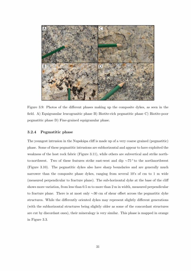
The last intrusive phase seen in the Nupskapa outcrop is a pegmatitic leucogranite phase,
which has intruded in several orientations. Some pegmatitic dykes are vertical and discordant,
while others are subhorizontal, and exploit the weakness of the host-rock fabric, as can be
seen in Figure 3.11. The pegmatitic phase appears to have intruded under somewhat different
conditions to the intrusion of the composite dyke phase, as their orientations are different.
The pegmatitic phase can be seen to intrude parallel to the gneissic fabric of the host rock, as
well as subvertically and discordant to the fabric. As the pegmatitic phase intruded after the
composite phase, the difference in orientation between the two is likely the result of the host
rocks sitting at shallower depths. With less depth and therefore less overburden, lower melt
pressure would be required for horizontal flow to occur. The differences in orientation may
also have resulted from a combination of changes in melt pressure, differential stress and the
orientation of the pre-existing weaknesses relative to the principle stresses. The pegmatitic
phase may also represent more than one intrusive event, with the more concordant features
having intruded under different conditions to the vertical ones (alhough there is no clear
mineralogical distinction between dykes with different orientations).
82
6.4 Implications for far-field melt transfer
The Nupskapa cliff represents an example of melt migration under mid-crustal conditions.
Melt transport appears to have occurred in numerous focused structures, that are spaced up
to 10 m apart and together form a pervasive intrusion of the country rock. The cliff also indi-
cates how melt accumulation can occur during transport and ascent in dyke-like structures.
Accumulation occurs via a gradual or step-wise process with smaller dykes coalescing and
feeding into larger dykes, which can exist parallel to each other for several tens or hundreds
of metres but may eventually join up to make larger structures.
This study shows an example of melt migration very different to the example described by
Diener et al. (2014). In the Aus granulite terrain in southern Namibia, these authors report
evidence of melt redistribution and accumulation occurring in the suprasolidus near-source
region. The implication of this is that melt batches entering the subsolidus crust would
be relatively large (on the order of several 10s of m3) and would already consist of several
smaller melt batches with differing compositions. The transition from pervasive to focused
migration is thought to occur in the near-source region, with large dykes initiating from the
large batches of accumulated melt (Rubin, 1995; Diener et al., 2014). Larger propagating
dykes would be less likely to become trapped by obstacles and further accumulation of melt
during ascent would not be required (Diener et al., 2014).
The style of melt migration represented by the composite dykes in the Nupskapa area
seems instead to have involved a gradual transition from pervasive to focused migration, with
intermittent accumulation occurring during transport. Smaller dyke structures coalesce into
larger ones, resulting in the mixing of melt batches en route. This reduces the need for, but
does not preclude, substantial accumulation in the near-source region.
The composite nature of the dykes indicates that the melt within them came from multiple
source areas, or a heterogeneous source. Whether these areas are distributed laterally or
vertically in space is hard to tell, but it is likely a combination of both (Figure 6.5). The
lack of consistent relative age relations amongst the different phases implies that the different
melt batches were contained simultaneously, not in separate pulses of different compositions.
Researchers (e.g Weertman, 1971; Bons et al., 2001, 2004; Brown, 2013) have suggested that
dykes are kept open by successive melt pulses, but this does not appear necessary for the
Nupskapa composite dykes. They appear to have had different melt phases moving through
them simultaneously, resulting in the disorganised leucosome phases now seen in the cliff. As
83
the dykes are thought to have intruded at temperatures significantly below the solidus, it is
unlikely that the different phases resulted from separate pulses of melt, with some of each
phase staying liquid long enough to mix with successive melt pulses within the dyke.
Figure 6.5: An idealised crustal-scale melt migration network, suggested by the composite
dyke phase in the Nupskapa area. Scale of melt-bearing structures indicated on left side.
84
6.5 Conclusions
The samples taken from the Nupskapa area show evidence of two equilibrium mineral as-
semblages. The ‘peak’ assemblage records metamorphic conditions of 820–880 ◦C at 9.5–
11.6 kbar. These granulite facies conditions are more than 100 ◦C higher than the Pan-African
peak conditions. They are much closer to the Grenvillian conditions identified in other parts
of H.U. Sverdrupfjella and the rest of the Maud Belt (Grantham et al., 1995; Groenewald
et al., 1995; Board et al., 2005). The area also preserves retrograde mineral assemblages,
which record metamorphic conditions of 555–595 ◦C at 3.2–4.8 kbar. As this assemblage is
preserved in these rocks it must post-date the last metamorphic event to have had tempera-
tures greater than 595 ◦C , otherwise a higher grade assemblage would be recorded instead.
Because the retrograde minerals show no preferred orientation, and based on dating by other
researchers, the retrograde conditions are interpreted as having a post-tectonic Pan-African
age (Board, 2001). These late M2 conditions lie between the wet solidus and brittle-viscous
transition and indicate a mid-crustal location, and the most likely conditions under which the
composite dykes were intruded. No direct evidence was found in the Nupskapa area for Pan-
African eclogite-facies conditions, as reported by Board (2001), although early Grenvillian
metamorphism may potentially have involved high-pressure granulite facies conditions.
The Nupskapa cliff shows evidence of multiple phases of melt intrusion. The oldest is
a concordant leucosome phase which is interpreted to represent initial melting and melt
segregation during M1 granulite-facies metamorphism. Younger, subvertical composite dykes
which cross-cut granulite fabric and concordant leucosome appear to have contained multiple
leucogranitic melt phases simultaneously. Melt migration through these structures is thought
to have occurred via tensile fracturing of the host rock, under conditions of low differential
stress and after the period of low-angle Pan-African thrusting had ceased to operate. It is
likely that melt pressure was sufficiently high to enable tensile fractures to propagate across
rocks of different grain size and composition, apparently irrespective of variations in strength
between the different rock types. The final intrusive phase is a pegmatitic leucogranite which
occurs in subvertical discordant structures as well as concordant structures that appear to
have exploited the subhorizontal foliation of the host rock. This phase is inferred to have
intruded at shallower conditions, and therefore lower pressures than the composite dyke phase
The composite dykes are inferred to represent an example of a gradual transition from
pervasive to focused migration. This transition appears to have occurred in the mid-crust, at
85
subsolidus temperatures, after the melt phases had been transported an estimated 5–15 km
from the source. This transition involves a network of smaller melt-filled fractures gradually
coalescing into larger ones which can then propagate further due to the increase in melt
volume (and therefore increased aperture as well as increased melt pressure). These larger
fractures may in turn have joined up at levels above this outcrop to make major dykes which
ultimately fed into emplacement structures at higher crustal levels. If pervasive migration
becomes focused via this gradual transition, melt accumulation and mixing need not occur
solely in the source or final emplacement structure, but rather occurs throughout transport
of the magma.
86
References
Anderson, E. M., 1951. The Dynamics of Faulting and Dyke Formation with Applications toBritain, Oliver & Boyd.
Arndt, N., Todt, W., Chauvel, C., Tapfer, M. & Weber, K., 1991. U-Pb zircon age and Nd iso-topic composition of granitoids, charnockites and supracrustal rocks from Heimefrontfjella,Antarctica. Geologische Rundschau, 80, 759–777.
Bateman, R., 1984. On the mechanics of igneous diapirism, stoping, and zone-melting -comment. American Journal of Science, 284(8), 979–980.
Beaumont, C., Jamieson, R., Butler, J. & Warren, C., 2009. Crustal structure: A keyconstraint on the mechanism of ultra-high-pressure rock exhumation. Earth and PlanetaryScience Letters, 287, 116–129.
Bisnath, A. & Frimmel, H. E., 2005. Metamorphic evolution of the Maud Belt: PTt pathfor high-grade gneisses in Gjelsvikfjella, Dronning Maud Land, East Antarctica. Journalof African Earth Sciences, 43, 505–524.
Bisnath, A., Frimmel, H. E., Armstrong, R. A. & Board, W. S., 2006. Tectono-thermalevolution of the Maud Belt: New SHRIMP U-Pb zircon data from Gjelsvikfjella, DronningMaud Land, East Antarctica. Precambrian Research, 150(1-2), 95–121.
Board, W. S., 2001. Tectonothermal evolution of the Southern H.U. Sverdrupfjella, WesternDronning Maud Land, Antarctica. PhD thesis, University of Cape Town.
Board, W. S., Frimmel, H. & Armstrong, R., 2005. Pan-African Tectonism in the WesternMaud Belt: P-T-t Path for High-grade Gneisses in the H.U. Sverdrupfjella, East Antarctica.Journal of Petrology, 46, 671–699.
Bons, P. D., Arnold, J., Elburg, M. A., Kaldad, J., Soesoo, A. & van Milligen, B. P., 2004.Melt extraction and accumulation from partially molten rocks. Lithos, 78, 25–42.
Bons, P. D., Druguet, E., Castano, L.-M. & Elburg, M. A., 2008. Finding what is now notthere anymore: Recognizing missing fluid and magma volumes. Geology, 36(11), 851–854.
Bons, P., Dougherty-Page, J. & Elburg, M., 2001. Stepwise accumulation and ascent ofmagmas. Journal of Metamorphic Geology, 19(5), 625–631.
Brown, M., 1994. The generation, segregation, ascent and emplacement of granite magma -The migmatite-to-crustally-derived-granite connection in thickened orogens. Earth-ScienceReviews, 36, 83–130.
Brown, M., 2004. The mechanism of melt extraction from lower continental crust of orogens.Transactions of the Royal Society of Edinburgh: Earth Sciences, 95(1-2), 35–48.
87
Brown, M., 2010. Melting of the continental crust during orogenesis: the thermal, rheological,and compositional consequences of melt transport from lower to upper continental crust.Canadian Journal of Earth Sciences, 47, 655–694.
Brown, M., 2013. Granite: From genesis to emplacement. Geological Society of AmericaBulletin, 125(7-8), 1079–1113.
Brown, M. & Solar, G., 1998a. Granite ascent and emplacement during contractional defor-mation in convergent orogens. Journal of Structural Geology, 20, 1365–1393.
Brown, M. & Solar, G., 1998b. Shear-zone systems and melts: feedback relations and self-organization in orogenic belts. Journal of Structural Geology, 20, 221–227.
Brown, M. & Solar, G., 1999. The mechanism of ascent and emplacement of granite magmaduring transpression: a syntectonic granite paradigm. Tectonophysics, 312, 1–33.
Brown, M., Korhonen, F. J. & Siddoway, C. S., 2011. Organizing Melt Flow through theCrust. Elements, 7, 261–266.
Clemens, J. & Mawer, C., 1992. Granitic magma transport by fracture propagation. Tectono-physics, 204, 339–360.
Clemens, J. & Vielzeuf, D., 1987. Constraints on melting and magma production in the crust.Earth and Planetary Science Letters, 86, 287–306.
Clemens, J., Petford, N. & Mawer, C., 1997. Ascent mechanisms of granitic magmas: causesand consequences.. In: Deformation-enhanced Fluid Transport in the Earth’s Crust andMantle, (ed. Holness, M. B.), pp. 145–172. Chapman & Hall for the Mineralogical SocietySeries.
Coggon, R. & Holland, T. J. B., 2002. Mixing properties of phengitic micas and revisedgarnet–phengite thermobarometers. Journal of Metamorphic Geology, 20, 683–696.
Collins, W. & Sawyer, E., 1996. Pervasive granitoid magma transfer through the lower-middle crust during non-coaxial compressional deformation. Journal of metamorphic Ge-ology, 14(5), 565–579.
Collins, W. J., Richards, S. R., Healy, B. E. & Ellison, P. I., 2000. Origin of heterogeneousmafic enclaves by two-stage hybridisation in magma conduits (dykes) below and in graniticmagma chambers. Earth and Environmental Science Transactions of the Royal Society ofEdinburgh, 91, 27–45.
Connolly, J. A. D. & Podladchikov, Y. Y., 2007. Decompaction weakening and channel-ing instability in ductile porous media: Implications for asthenospheric melt segregation.Journal of Geophysical Research, 112, B10205.
Diener, J. F. A. & Powell, R., 2012. Revised activity–composition models for clinopyroxeneand amphibole. Journal of Metamorphic Geology, 30, 131–142.
Diener, J. F. A., Powell, R., White, R. W. & Holland, T. J. B., 2007. A new thermodynamicmodel for clino- and orthoamphiboles in the system Na2O–CaO–FeO–MgO–Al2O3–SiO2–H2O–O. Journal of Metamorphic Geology, 25, 631–656.
88
Diener, J. F., White, R. W. & Hudson, T. J., 2014. Melt production, redistribution andaccumulation in mid-crustal source rocks, with implications for crustal-scale melt transfer.Lithos, 200-201, 212–225.
Diener, J., White, R. & Powell, R., 2008. Granulite facies metamorphism and subsolidusfluid-absent reworking, Strangways Range, Arunta Block, central Australia. Journal ofMetamorphic Geology, 26, 603622.
Etheridge, M., 1983. Differential stress magnitudes during regional deformation and meta-morphism - upper bound imposed by tensile fracturing. Geology, 11(4), 231–234.
Faber, C., (2012). Processes of felsic melt migration through the mid-crust: evidence fromfield relations in the central zone of the damara belt, namibia, Master’s thesis, Universityof Cape Town.
Fitzsimons, I., 2000a. A review of tectonic events in the East Antarctic Shield and theirimplications for Gondwana and earlier supercontinents. Journal of African Earth Sci-ences, 31, 3–23.
Fitzsimons, I., 2000b. Grenville-age basement provinces in East Antarctica: Evidence forthree separate collisional orogens. Geology, 28(10), 879–882.
Grantham, G., 1992. Geological evolution of western H.u. Sverdrupfje/la, Dronning MaudLand, Antarctica. PhD thesis, University of Natal, Pietermaritzburg.
Grantham, G. H., Jackson, C., Moyes, A. B., Groenewald, P. B., Harris, P. D., Ferrar, G. &Krynauw, J. R., 1995. The tectonothermal evolution of the KirwanveggenH.U. Sverdrupf-jella areas, Dronning Maud Land, Antarctica. Precambrian Research, 75, 209–229.
Grantham, G.H., G. P. & Hunter, D., 1988. Geology of the northern h.u. sverdrupfjella,western dronning maud land, and implications for gondwana reconstructions. South AfricanJournal of Antarctic Research, 18, 2–10.
Green, E. C. R., Holland, T. J. B. & Powell, R., 2007. An order–disorder model for om-phacitic pyroxenes in the system jadeite–diopside–hedenbergite–acmite, with applicationsto eclogitic rocks. American Mineralogist, 92, 1181–1189.
Groenewald, P. B. & Hunter, D. R., 1991. Granulites of the northern H.U. Sverdrupfjella,western Dronning Maud Land: Metamorphic history from garnetpyroxene assemblages,coronas and hydration reactions. In: Geological Evolution of Antarctica., (eds Thomson,M. R. A., Crame, J. A. & Thomson, J. W.). Cambridge University Press.
Groenewald, P. B., Moyes, A. B., Grantham, G. H. & Krynauw, J. R., 1995. East Antarcticcrustal evolution: Geological constraints and modelling in western Dronning Maud Land.Precambrian Research, 75, 231–250.
Groenewald, P., Grantham, G. & Watkeys, M., 1991. Geological evidence for a Proterozoic toMesozoic link between Southeastern Africa and Dronning Maud Land, Antarctica. Journalof the Geological Society, 148(6), 1115–1123.
Hall, D. & Kisters, A., 2012. The stabilization of self-organised leucogranite networksImpli-cationsfor melt segregation and far-field melt transfer in the continental crust. Earth andPlanetary Science Letters, 355-356, 1–12.
89
Handy, M., Braun, J., Brown, M., Kukowski, N., Paterson, M., Schmid, S., Stockhert, B.,Stuwe, K., Thompson, A. & Wosnitza, E., 2001. Rheology and geodynamic modelling: thenext step forward. International Journal of Earth Sciences, 90(1), 149–156.
Harris, C. & Grantham, G., 1993. Geology and petrogenesis of the Straumsvola nephelinesyenite complex, Dronning Maud Land, Antarctica. Geological Magazine, 130, 523–532.
Harris, P., Moyes, A., Fanning, C. & Armstrong, R., 1995. Zircon ion microprobe resultsfrom the Maudheim high-grade gneiss terrane, western Dronning Maud Land, Antarctica.Extended Abstracts, Centennial Geocongress, Rand Afrikaans University, Johannesburg,South Africa, pp. 240–243.
Harrison, T. & Fitzgerald, J., 1986. Exsolution in hornblende and its consequences for 40Ar–39Ar age spectra and closure temperature. Geochimica et Cosmochimica Acta, 50, 247–253.
Hjelle, A., 1974. Some observations on the geology of the H.U. Sverdrupfjella, DronningMaud Land, Antarctica. Norsk Polarinstitutt., Arbor 1972, 7–22.
Holland, T. J. B. & Powell, R., 1998. An internally consistent thermodynamic dataset forphases of petrological interest. Journal of Metamorphic Geology, 16, 309–343.
Holland, T. J. B. & Powell, R., 2003. Activity–composition relations for phases in petrologicalcalculations: an asymmetric multicomponent formulation. Contributions to Mineralogy andPetrology, 145, 492–501.
Holland, T. J. B., Baker, J. M. & Powell, R., 1998. Mixing properties and activity–composition relationships of chlorites in the system MgO–FeO–Al2O3–SiO2–H2O . Eu-ropean Journal of Mineralogy, 10, 395–406.
Hollister, L. S. & Crawford, M. L., 1986. Melt-enhanced deformation: A major tectonicprocess. Geology, 14, 558–561.
Ito, G. & Martel, S., 2002. Focusing of magma in the upper mantle through dike interaction.Journal Of Geophysical Research-Solid Earth, 107(B10).
Jamieson, R. & Beaumont, C., 2011. Coeval thrusting and extension during lower crustalductile flow implications for exhumation of high-grade metamorphic rocks. Journal ofmetamorphic Geology, 29, 33–51.
Kisters, A., Ward, R., Anthonissen, C. & Vietze, M., 2009. Melt segregation and far-fieldmelt transfer in the mid-crust. Journal of the Geological Society, 166, 905–918.
Leitch, A. & Weinberg, R., 2002. Modelling granite migration by mesoscale pervasive flow.Earth and Planetary Science Letters, 200(1-2), 131–146.
Lister, J. & Kerr, R., 1991. Fluid-mechanical models of crack-propagation and their applica-tion to magma transport in dykes. Journal of Geophysical Research, 96(B6), 10049–10077.
Mahon, K., Harrison, T. & Drew, D., 1988. Ascent of a granitoid diapir in a temperaturevarying medium. Journal of Geophysical Research, B93, 1174–1188.
Marsh, B. D., 1982. On the mechanics of igneous diapirism, stoping and zone melting.American Journal of Science, 282, 808–855.
90
McGibbon, D., 2014. Shear Zones of the Maud Belt, Antarctica: Kinematics and DeformationMechanisms. PhD thesis, University of Cape Town.
McNulty, B., Tobisch, O. T., Cruden, A. R. & Gilder, S., 2000. Multistage emplacement ofthe Mount Givens pluton, central Sierra Nevada batholith, California. Geological Societyof America Bulletin, 112, 119–135.
Morfin, S., Sawyer, E. W. & Bandyayera, D., 2013. Large volumes of anatectic melt retainedin granulite facies migmatites: An injection complex in northern Quebec. Lithos, 168, 200–218.
Ohta, Y., (1996). 1996: Nature environment map, h.u. sverdrupfjella 1:150000, Technicalreport, Norsk Polarinstitutt Temakart Nr. 28.
Paterson, S. & Vernon, R., 1995. Bursting the bubble of ballooning plutons - a returnto nested diapirs emplaced by multiple processes. Geological Society of America Bul-letin, 107(11), 1356–1380.
Paterson, S. R. & Fowler, T., 1993. Re-examining pluton emplacement processes. Journal ofStructural Geology, 15, 191–206.
Paulsson, O. & Austrheim, H., 2003. A geochronological and geochemical study of rocksfrom Gjelsvikfjella, Dronning Maud Land, Antarctica - implications for Mesoproterozoiccorrelations and assembly of Gondwana. Precambrian Research, 125(1-2), 113–138.
Petford, N., 1996. Dykes or Diapirs? Transactions of the Royal Society of Edinburgh: EarthSciences, 87, 105–114.
Petford, N., Kerr, R. & Lister, J., 1993. Dike transport of granitoid magmas. Geol-ogy, 21(9), 845–848.
Petford, N., Lister, J. & Kerr, R., 1994. The ascent of felsic magmas in dykes. Lithos, 32(1-2), 161–168.
Reichardt, H. & Weinberg, R. E., 2012. The dike swarm of the Karakoram shear zone,Ladakh, NW India: Linking granite source to batholith. Geological Society of AmericaBulletin, 124(1-2), 89–103.
Rubin, A., 1995. Propagation of magma-filled cracks. Annual Review of Earth And PlanetarySciences, 23, 287–336.
Sawyer, E. W., 1994. Melt Segregation in the continental crust. The Geological Society ofAmerica, 22, 1019–1022.
Sawyer, E. W., Cesare, B. & Brown, M., 2011. When the Continental Crust Melts. Ele-ments, 7, 220–234.
Schulmann, K., Lexa, O., Stipska, P., Racek, M., Tajcmanova, L., Konopasek, J., Edel, J.,Peschler, A. & Lehmann, J., 2008. Vertical extrusion and horizontal channel flow of orogeniclower crust: key exhumation mechanisms in large hot orogens? Journal of MetamorphicGeology, 26, 273–297.
Sebetlela, T., (2013). Geometry and deformation mechanisms of a polydeformed retrogradeshear zone of the Maud Belt, Antarctica, Honours thesis, University of Cape Town.
91
Sleep, N., 1988. Tapping of melt by veins and dikes. Journal of Geophysical Re-search, 93(B9), 10255–10272.
Spear, F. S., 1995. Metamorphic Phase Equilibria And Presure-Temperature-Time-Paths,Mineralogical Society of America Monograph.
Stevens, G., Clemens, J. & Droop, G. T., 1997. Melt production during granulite-faciesanatexis: experimental data from ’primitive’ metasedimentary protoliths. Contributions toMineralogy and Petrology, 128, 352–370.
Sweeney, J., 1975. Diapiric granite batholiths in south-central Maine. American Journal ofScience, 275(10), 1183–1191.
Vanderhaeghe, O., 2001. Melt Segregation, Pervasive Melt Migration and Magma Mobilityin the Continental Crust: The Structural Record from Pores to Orogens. Physics andChemistry of the Earth, 26, 213–223.
Vermilye, J. M. & Scholz, C. H., 1995. Relation between vein length and aperture. Journalof Structural Geology, 17, 423–434.
Vernon, R. H. & Paterson, S. R., 2001. Axial-surface leucosomes in anatectic migmatites.Tectonophysics, 335., 183–192.
Vielzeuf, D. & Schmidt, M., 2001. Melting relations in hydrous systems revisited: applica-tion to metapelites, metagreywackes and metabasalts. Contributions to Mineralogy andPetrology, 141, 251–267.
Vigneresse, J. L., 2006. Granitic batholiths: from pervasive and continuous melting in thelower crust to discontinuous and spaced plutonism in the upper crust. Transactions of theRoyal Society of Edinburgh: Earth Sciences, 97, 311–324.
Weertman, J., 1971. Theory of water-filled crevasses in glaciers applied to vertical magmatransport beneath oceanic ridges. Journal of Geophysical Research, 76, 1171–1183.
Weinberg, R. & Podladchikov, Y., 1994. Diapiric ascent of magmas through power law crustand mantle. Journal of Geophysical Research, 99, 9543–9559.
Weinberg, R. F., 1996. Ascent of felsic magmas: news and reviews. Transactions of the RoyalSociety of Edinburgh: Earth Sciences, 87, 95–103.
Weinberg, R. F., 1999. Mesoscale pervasive felsic magma migration: alternatives to dyking.Lithos, 46, 393–410.
Weinberg, R. F. & Regenauer-Lieb, K., 2010. Ductile fractures and magma migration fromsource. Geology, 38(4), 363–366.
White, R. & Powell, R., 2002. Melt loss and the preservation of granulite facies mineralassemblages. Journal of Metamorphic Geology, 20, 621632.
White, R., Powell, R. & Halpin, J., 2004. Spatially-focussed melt formation in aluminousmetapelites from Broken Hill, Australia. Journal of Metamorphic Geology, 22, 825845.
White, R. W., Powell, R. & Clarke, G. L., 2002. The interpretation of reaction textures in Fe-rich metapelitic granulites of the Musgrave Block, central Australia: constraints from min-eral equilibria calculations in the system K2O–FeO–MgO–Al2O3–SiO2–H2O–TiO2–Fe2O3.Journal of Metamorphic Geology, 20, 41–55.
92
White, R. W., Powell, R. & Holland, T. J. B., 2007. Progress relating to calculation of partialmelting equilibria for metapelites. Journal of Metamorphic Geology, 25, 511–527.
White, W., Powell, R., Holland, T. J. B. & Worley, B. A., 2000. The effect of TiO2 andFe2O3 on metapelitic assemblages at greenschist and amphibolite facies conditions: min-eral equilibria calculations in the system K2O–FeO–MgO–Al2O3–SiO2–H2O–TiO2–Fe2O3.Journal of Metamorphic Geology, 18, 497–511.
Whitney, P. R. & McLelland, J. M., 1983. Origin of Biotite-Hornblende-Garnet Coronasbetween Oxides and Plagioclase in Olivine Metagabbros, Adirondack Region, New York.Contributions to Mineralogy and Petrology, 82, 34–41.
93
Tab
leA
.1:
Ele
ctro
nm
icro
pro
be
resu
lts
for
garn
etin
all
sam
ple
s
S01-1
S01-2
S01-3
S01-4
S01-5
S01-6
S01-7
S01-8
S01-9
S01-1
0S
01-1
1S
01-1
2S
01-1
3
SiO
238
.85
37.3
137
.41
37.6
937
.40
37.5
736
.67
36.5
546.2
936.7
736.8
836.7
536.5
2T
iO2
0.06
0.04
0.05
0.03
0.01
0.09
0.08
0.05
0.0
00.0
20.0
40.0
60.0
7A
l 2O
318
.88
21.8
022
.02
22.3
021
.80
22.0
421
.69
21.8
15.4
521.9
522.0
021.9
121.6
3C
r 2O
30.
020.
000.
010.
000.
030.
040.
060.
00
0.0
00.0
20.0
10.0
00.0
2FeO
32.9
532
.44
31.2
529
.29
31.4
730
.37
33.0
532
.54
35.2
632.1
232.0
732.0
432.9
9M
nO
1.42
1.49
1.31
1.15
1.37
1.24
1.79
1.71
0.7
41.7
11.5
81.5
01.6
0M
gO
4.11
2.54
3.15
3.15
2.71
3.11
2.13
2.40
11.6
02.2
72.5
32.7
02.2
1C
aO
6.26
6.48
7.28
9.07
7.67
8.01
6.59
6.84
1.6
77.3
77.0
46.8
26.9
0N
a2O
0.06
0.02
0.01
0.02
0.03
0.00
0.04
0.03
0.0
00.0
80.0
40.0
30.0
6
Tota
l10
2.61
102.
1310
2.50
102.
7010
2.49
102.
4710
2.10
101.9
3101.0
1102.3
2102.1
9101.8
1102.0
0
Oxygen
s24
2424
2424
2424
2424
24
24
24
24
Si
6.10
5.88
5.85
5.85
5.86
5.86
5.82
5.80
7.3
45.8
05.8
15.8
15.8
0T
i0.
010.
010.
010.
000.
000.
010.
010.
01
0.0
00.0
00.0
00.0
10.0
1A
l3.
494.
054.
064.
084.
034.
054.
054.
08
1.0
24.0
84.0
94.0
84.0
5C
r0.
000.
000.
000.
000.
000.
000.
010.
00
0.0
00.0
00.0
00.0
00.0
0Fe
4.33
4.27
4.08
3.80
4.12
3.96
4.38
4.32
4.6
74.2
44.2
34.2
44.3
8M
n0.
190.
200.
170.
150.
180.
160.
240.
23
0.1
00.2
30.2
10.2
00.2
2M
g0.
960.
600.
730.
730.
630.
720.
500.
57
2.7
40.5
30.5
90.6
40.5
2C
a1.
051.
091.
221.
511.
291.
341.
121.
16
0.2
81.2
51.1
91.1
61.1
7N
a0.
020.
010.
000.
010.
010.
000.
010.
01
0.0
00.0
20.0
10.0
10.0
2
Tota
l16
.15
16.1
016
.12
16.1
216
.13
16.1
116
.15
16.1
616.1
516.1
616.1
416.1
416.1
7
...c
onti
nu
edon
nex
tp
age
95
Tab
leA
.1G
arn
et
–co
nti
nu
edfr
omp
revio
us
pag
e
S01-1
4S
01-1
5S
01-1
6S
01-1
7S
01-1
8S
01-1
9S
10-2
S10-3
S10-4
S10-5
s52-1
s52-2
s52-3
10p
tS
iO2
36.6
146
.29
35.7
235
.76
47.1
435
.96
35.4
535
.82
36.0
736.0
540.3
539.9
439.6
9T
iO2
0.08
0.04
0.06
0.00
0.06
0.12
0.13
0.09
0.0
50.0
40.0
90.0
50.0
3A
l 2O
321
.98
4.02
21.8
321
.69
1.16
21.1
121
.13
21.1
120.9
321.4
621.8
421.5
621.5
0C
r 2O
30.
000.
010.
000.
000.
000.
010.
020.
00
0.0
20.0
40.0
00.0
10.0
2FeO
32.8
037
.30
33.1
034
.17
38.9
228
.82
27.9
527
.86
28.0
125.1
829.9
130.0
527.6
7M
nO
1.39
0.67
1.69
1.67
0.59
1.29
1.66
1.99
2.0
25.9
41.1
30.7
13.3
9M
gO
2.42
11.1
52.
132.
2711
.82
1.75
1.55
1.75
1.8
11.0
01.7
01.9
50.8
5C
aO
6.85
1.10
6.90
5.65
0.53
11.5
511
.42
11.2
211.2
310.1
89.7
110.0
410.3
9N
a2O
0.06
0.03
0.01
0.00
0.05
0.04
0.10
0.07
0.0
40.1
10.0
10.1
00.0
0
Tota
l10
2.19
100.
6010
1.44
101.
2210
0.28
100.
6599
.41
99.9
1100.1
7100.0
0104.7
3104.4
1103.5
4
Oxygen
s24
2424
2424
2424
2424
24
24
24
24
Si
5.79
7.44
5.72
5.75
7.66
5.77
5.75
5.78
5.8
15.8
26.1
26.0
86.1
1T
i0.
010.
000.
010.
000.
010.
010.
020.
01
0.0
10.0
00.0
10.0
10.0
0A
l4.
100.
764.
124.
110.
223.
994.
044.
01
3.9
74.0
83.9
03.8
73.9
0C
r0.
000.
000.
000.
000.
000.
000.
000.
00
0.0
00.0
10.0
00.0
00.0
0Fe
4.34
5.01
4.43
4.59
5.29
3.86
3.79
3.76
3.7
73.4
03.7
93.8
33.5
6M
n0.
190.
090.
230.
230.
080.
170.
230.
27
0.2
80.8
10.1
40.0
90.4
4M
g0.
572.
670.
510.
542.
860.
420.
380.
42
0.4
30.2
40.3
80.4
40.1
9C
a1.
160.
191.
180.
970.
091.
981.
991.
94
1.9
41.7
61.5
81.6
41.7
1N
a0.
020.
010.
000.
000.
020.
010.
030.
02
0.0
10.0
30.0
00.0
30.0
0
Tota
l16
.16
16.1
816
.21
16.2
016
.23
16.2
316
.23
16.2
116.2
116.1
515.9
315.9
915.9
3
...c
onti
nu
edon
nex
tp
age
96
Tab
leA
.1G
arn
et
–co
nti
nu
edfr
omp
revio
us
pag
e
s52-4
s52-5
s52-6
s52-7
s52-9
s52-1
0s6
4-1
s64-2
s64-3
s62-1
s62-2
s62-3
s62-4
10p
tS
iO2
39.8
339
.99
37.4
737
.38
37.0
236
.27
36.7
736
.92
36.4
835.4
135.1
534.5
039.3
3T
iO2
0.05
0.07
0.08
0.06
0.03
0.04
0.02
0.04
0.0
30.0
30.0
30.0
00.0
0A
l 2O
321
.69
21.6
621
.79
21.9
021
.46
21.4
421
.99
22.0
521.7
422.0
321.9
721.8
121.4
4C
r 2O
30.
010.
010.
000.
000.
000.
000.
000.
04
0.0
00.0
40.0
10.0
00.0
2FeO
29.1
429
.66
29.4
630
.18
29.5
729
.16
34.7
534
.58
34.0
934.0
033.0
132.9
032.9
2M
nO
0.60
2.24
0.57
0.63
1.67
0.74
4.37
4.21
4.4
45.5
77.1
67.0
66.8
8M
gO
2.24
1.21
2.04
2.09
1.34
1.86
2.98
2.90
3.0
02.5
02.0
82.0
82.0
8C
aO
10.1
09.
6610
.02
9.38
10.0
211
.11
1.58
1.85
1.4
11.1
01.0
81.0
61.2
2N
a2O
0.00
0.06
0.06
0.01
0.03
0.05
0.01
0.01
0.0
40.0
50.0
50.0
00.0
4
Tota
l10
3.66
104.
5610
1.50
101.6
310
1.14
100.
6710
2.47
102.
59
101.2
3100.7
3100.5
499.4
1103.9
3
Oxygen
s24
2424
24
2424
2424
24
24
24
24
24
Si
6.08
6.10
5.90
5.88
5.89
5.79
5.83
5.84
5.8
55.7
45.7
35.7
06.1
1T
i0.
010.
010.
010.
010.
000.
010.
000.
00
0.0
00.0
00.0
00.0
00.0
0A
l3.
903.
894.
044.
064.
024.
044.
114.
11
4.1
14.2
14.2
24.2
53.9
3C
r0.
000.
000.
000.
000.
000.
000.
000.
00
0.0
00.0
10.0
00.0
00.0
0Fe
3.72
3.78
3.88
3.97
3.93
3.90
4.61
4.57
4.5
74.6
14.5
04.5
44.2
8M
n0.
080.
290.
080.
080.
220.
100.
590.
56
0.6
00.7
70.9
90.9
90.9
1M
g0.
510.
280.
480.
490.
320.
440.
700.
68
0.7
20.6
00.5
10.5
10.4
8C
a1.
651.
581.
691.
581.
711.
900.
270.
31
0.2
40.1
90.1
90.1
90.2
0N
a0.
000.
020.
020.
000.
010.
020.
000.
00
0.0
10.0
10.0
20.0
00.0
1
Tota
l15
.96
15.9
516
.08
16.0
816
.10
16.1
916
.11
16.1
016.1
016.1
516.1
616.1
815.9
3
...c
onti
nu
edon
nex
tp
age
97
Tab
leA
.1G
arn
et
–co
nti
nu
edfr
omp
revio
us
pag
e
s62-5
s50-1
s50-2
s50-3
s50-4
s50-6
s50-7
s50-8
s50-9
s50-1
0s5
5-1
s55-2
s55-3
SiO
239
.36
39.5
138
.79
39.3
538
.48
39.7
839
.31
38.9
538.8
138.4
538.6
038.0
838.3
5T
iO2
0.00
0.05
0.02
0.09
0.01
0.08
0.06
0.06
0.0
70.0
40.0
30.0
60.0
9A
l 2O
321
.42
21.3
621
.42
21.4
721
.02
21.3
421
.50
21.6
621.5
721.7
621.7
921.6
521.6
3C
r 2O
30.
010.
010.
000.
010.
060.
000.
030.
00
0.0
00.0
40.0
00.0
00.0
5FeO
32.8
729
.82
30.4
629
.37
29.5
929
.59
30.2
129
.41
30.3
629.4
130.5
429.7
830.6
2M
nO
6.53
0.73
2.03
0.52
2.23
0.49
1.81
0.63
1.6
40.6
50.6
02.6
00.8
3M
gO
2.32
2.34
1.21
2.50
1.05
2.53
1.17
2.45
1.4
92.5
72.3
41.1
81.9
2C
aO
1.12
9.55
9.09
9.70
9.02
9.80
9.27
9.67
9.0
49.7
49.4
19.3
79.6
2N
a2O
0.05
0.00
0.04
0.05
0.10
0.01
0.03
0.06
0.0
10.0
40.0
20.0
20.0
4
Tota
l10
3.67
103.
3710
3.05
103.
0610
1.55
103.
6310
3.38
102.8
9102.9
9102.7
0103.3
4102.7
4103.1
5
Oxygen
s24
2424
2424
2424
2424
24
24
24
24
Si
6.12
6.07
6.04
6.06
6.07
6.09
6.08
6.01
6.0
35.9
65.9
65.9
65.9
5T
i0.
000.
010.
000.
010.
000.
010.
010.
01
0.0
10.0
00.0
00.0
10.0
1A
l3.
933.
873.
933.
893.
913.
853.
923.
94
3.9
53.9
73.9
73.9
93.9
6C
r0.
000.
000.
000.
000.
010.
000.
000.
00
0.0
00.0
00.0
00.0
00.0
1Fe
4.27
3.83
3.96
3.78
3.90
3.79
3.91
3.80
3.9
43.8
13.9
43.8
93.9
7M
n0.
860.
100.
270.
070.
300.
060.
240.
08
0.2
20.0
90.0
80.3
40.1
1M
g0.
540.
540.
280.
570.
250.
580.
270.
56
0.3
50.5
90.5
40.2
80.4
4C
a0.
191.
571.
521.
601.
521.
611.
541.
60
1.5
01.6
21.5
61.5
71.6
0N
a0.
010.
000.
010.
020.
030.
000.
010.
02
0.0
00.0
10.0
10.0
10.0
1
Tota
l15
.92
15.9
916
.00
16.0
015
.99
15.9
815
.96
16.0
215.9
916.0
616.0
616.0
416.0
6
...c
onti
nu
edon
nex
tp
age
98
Tab
leA
.1G
arn
et
–co
nti
nu
edfr
omp
revio
us
pag
e
s55-4
s55-5
s55-6
s55-7
s55-8
s55-9
s65-1
s65-2
s65-3
s65-4
s65-5
s65-6
s67-1
SiO
238
.39
37.8
437
.46
37.3
037
.35
37.5
938
.94
38.5
338.5
138.3
038.4
238.2
837.8
1T
iO2
0.02
0.05
0.03
0.07
0.07
0.05
0.00
0.01
0.0
30.0
60.0
00.0
00.0
6A
l 2O
321
.80
21.8
921
.72
21.8
521
.26
21.6
922
.67
22.7
822.8
222.7
722.6
822.5
521.8
6C
r 2O
30.
010.
010.
030.
010.
000.
010.
140.
11
0.0
60.1
20.0
90.1
10.0
8FeO
29.9
930
.48
27.8
931
.47
29.7
930
.67
24.9
426
.04
26.7
825.8
727.2
328.0
026.7
0M
nO
2.28
0.62
3.79
0.79
2.89
0.60
1.08
1.05
1.7
61.0
71.6
92.0
50.9
0M
gO
1.22
2.01
0.71
1.77
0.95
1.95
8.47
7.87
6.3
87.1
76.5
66.1
34.3
5C
aO
9.64
9.58
10.4
89.
4310
.17
9.48
4.95
4.89
5.2
05.7
15.1
74.9
88.1
6N
a2O
0.00
0.05
0.74
0.04
0.05
0.03
0.02
0.01
0.0
40.0
20.0
20.0
10.0
0
Tota
l10
3.35
102.
5310
2.85
102.
7210
2.54
102.
0710
1.21
101.3
0101.5
8101.0
9101.8
6102.1
199.9
1
Oxygen
s24
2424
2424
2424
2424
24
24
24
24
Si
5.96
5.91
5.88
5.85
5.89
5.90
5.92
5.88
5.9
15.8
85.8
95.8
85.9
4T
i0.
000.
010.
000.
010.
010.
010.
000.
00
0.0
00.0
10.0
00.0
00.0
1A
l3.
994.
034.
024.
043.
954.
014.
064.
10
4.1
24.1
24.1
04.0
84.0
5C
r0.
000.
000.
000.
000.
000.
000.
020.
01
0.0
10.0
10.0
10.0
10.0
1Fe
3.90
3.98
3.66
4.13
3.93
4.03
3.17
3.33
3.4
33.3
23.4
93.6
03.5
1M
n0.
300.
080.
500.
100.
390.
080.
140.
14
0.2
30.1
40.2
20.2
70.1
2M
g0.
280.
470.
170.
410.
220.
461.
921.
79
1.4
61.6
41.5
01.4
01.0
2C
a1.
601.
601.
761.
581.
721.
590.
810.
80
0.8
50.9
40.8
50.8
21.3
7N
a0.
000.
020.
230.
010.
020.
010.
010.
00
0.0
10.0
10.0
00.0
00.0
0
Tota
l16
.04
16.0
816
.22
16.1
316
.13
16.0
916
.04
16.0
616.0
316.0
516.0
616.0
716.0
2
...c
onti
nu
edon
nex
tp
age
99
Tab
leA
.1G
arn
et
–co
nti
nu
edfr
omp
revio
us
pag
e
s67-2
s67-3
s67-4
s67-5
s67-6
s67-7
s67-8
s67-9
s67-1
0s6
7-1
1s6
7-1
2s6
7-1
3
SiO
237
.75
37.8
437
.81
37.3
537
.40
37.6
637
.75
37.7
337.4
537.2
137.2
837.9
9T
iO2
0.01
0.07
0.04
0.03
0.04
0.03
0.03
0.04
0.0
60.0
40.0
10.0
9A
l 2O
321
.65
23.2
922
.32
21.7
421
.72
21.9
321
.91
22.1
121.6
921.7
321.7
121.9
5C
r 2O
30.
080.
000.
010.
000.
090.
000.
020.
06
0.0
50.0
00.0
70.0
5FeO
28.4
824
.30
26.5
228
.12
27.7
227
.31
27.8
726
.00
28.2
928.5
728.3
026.9
4M
nO
1.89
0.95
0.90
2.20
1.98
1.61
1.54
0.74
2.0
21.9
72.3
80.9
1M
gO
3.50
3.33
4.53
3.05
3.20
3.29
3.67
5.00
3.3
43.2
42.8
84.2
4C
aO
6.84
9.44
8.28
6.81
7.72
8.52
7.83
8.50
7.2
07.4
26.9
88.5
6N
a2O
0.04
0.07
0.01
0.01
0.06
0.03
0.03
0.06
0.0
00.0
20.0
00.0
2
Tota
l10
0.24
99.2
910
0.42
99.3
199
.93
100.
3910
0.64
100.
24
100.1
0100.2
099.6
1100.7
5
Oxygen
s24
2424
2424
2424
2424
24
24
24
Si
5.97
5.93
5.90
5.96
5.93
5.93
5.93
5.89
5.9
35.9
05.9
55.9
3T
i0.
000.
010.
010.
000.
000.
000.
000.
01
0.0
10.0
10.0
00.0
1A
l4.
034.
304.
114.
094.
064.
074.
064.
07
4.0
54.0
64.0
84.0
4C
r0.
010.
000.
000.
000.
010.
000.
000.
01
0.0
10.0
00.0
10.0
1Fe
3.76
3.18
3.46
3.75
3.68
3.60
3.66
3.40
3.7
53.7
93.7
73.5
2M
n0.
250.
130.
120.
300.
270.
210.
200.
10
0.2
70.2
60.3
20.1
2M
g0.
820.
781.
050.
730.
760.
770.
861.
16
0.7
90.7
70.6
80.9
9C
a1.
161.
581.
381.
161.
311.
441.
321.
42
1.2
21.2
61.1
91.4
3N
a0.
010.
020.
000.
000.
020.
010.
010.
02
0.0
00.0
10.0
00.0
1
Tota
l16
.02
15.9
316
.04
15.9
916
.04
16.0
416
.04
16.0
716.0
316.0
616.0
116.0
4
100
Tab
leA
.2:
Ele
ctro
nm
icro
pro
be
resu
lts
for
am
ph
ibole
S01-1
S01-2
S01-3
S01-4
S01-5
S01-6
S01-7
S01-8
S01-9
S01-1
0S
01-1
3S
01-1
4S
01-1
5
SiO
241
.06
41.0
741
.19
41.3
140
.28
40.5
940
.63
38.9
041.9
540.5
140.6
940.6
740.9
5T
iO2
1.88
1.87
1.76
1.56
1.80
2.06
2.19
1.5
91.6
71.3
51.7
11.6
41.6
2A
l 2O
312
.97
12.8
113
.14
12.9
314
.64
13.9
213
.47
11.6
312.3
614.3
012.7
012.9
913.3
6C
r 2O
30.
000.
010.
010.
000.
000.
050.
020.0
00.0
30.0
00.0
00.0
00.0
0FeO
21.8
721
.47
21.7
521
.27
19.7
719
.80
20.1
718.6
620.2
620.2
421.5
621.7
321.6
2M
nO
0.16
0.13
0.20
0.16
0.16
0.14
0.14
0.1
10.0
80.0
80.1
40.1
70.2
4M
gO
7.69
7.73
7.86
8.47
8.25
8.35
8.44
8.5
59.1
08.3
07.7
57.8
17.9
5C
aO
10.9
910
.89
10.8
410
.82
11.3
111
.32
11.2
110.4
711.4
111.4
410.9
211.0
710.8
2N
a2O
2.37
2.41
2.46
2.50
2.59
2.61
2.50
2.2
82.3
92.6
02.4
22.4
62.4
7K
2O
0.91
0.85
0.81
0.67
0.64
0.69
0.79
0.6
30.7
00.6
80.7
00.6
70.6
8
Tota
l99
.90
99.2
310
0.01
99.6
999
.44
99.5
399
.56
92.8
399.9
699.5
098.5
999.2
199.7
1
Oxygen
s23
2323
2323
2323
23
23
23
23
23
23
Si
6.20
6.23
6.20
6.22
6.05
6.10
6.11
6.2
66.2
76.0
96.2
16.1
86.1
8T
i0.
210.
210.
200.
180.
200.
230.
250.1
90.1
90.1
50.2
00.1
90.1
8A
l2.
312.
292.
332.
292.
592.
462.
392.2
02.1
82.5
32.2
92.3
32.3
7C
r0.
000.
000.
000.
000.
000.
010.
000.0
00.0
00.0
00.0
00.0
00.0
0Fe
2.76
2.72
2.74
2.68
2.48
2.49
2.54
2.5
12.5
32.5
52.7
52.7
62.7
3M
n0.
020.
020.
020.
020.
020.
020.
020.0
10.0
10.0
10.0
20.0
20.0
3M
g1.
731.
751.
761.
901.
851.
871.
892.0
52.0
31.8
61.7
61.7
71.7
9C
a1.
781.
771.
751.
741.
821.
821.
811.8
01.8
31.8
41.7
91.8
01.7
5N
a0.
690.
710.
720.
730.
750.
760.
730.7
10.6
90.7
60.7
20.7
20.7
2K
0.17
0.16
0.16
0.13
0.12
0.13
0.15
0.1
30.1
30.1
30.1
40.1
30.1
3
Tota
l15
.87
15.8
515
.87
15.8
915
.89
15.8
815
.89
15.8
715.8
615.9
315.8
715.9
015.8
8
...c
onti
nu
edon
nex
tp
age
101
Tab
leA
.2A
mp
hib
ole
s–
conti
nu
edfr
omp
revio
us
pag
e
S01-1
6S
01-1
7S
01-1
8S
01-2
0S
01-2
1S
01-2
2S
01-2
3S
01-2
4S
01-2
5S
01-2
6S
01-2
7S
01-2
8S
01-2
9
SiO
240
.85
41.5
541
.18
41.6
640
.86
40.5
939
.92
41.2
040.2
834.7
639.7
739.5
739.6
6T
iO2
1.62
1.35
0.90
1.23
1.50
1.66
1.48
1.4
01.5
03.6
81.5
31.8
11.5
6A
l 2O
313
.30
12.8
513
.71
12.6
112
.64
13.1
714
.21
12.9
912.4
915.8
212.9
512.9
912.8
3C
r 2O
30.
050.
000.
000.
000.
010.
000.
000.0
40.0
00.0
00.0
30.0
00.0
3FeO
21.4
420
.77
19.9
822
.58
22.1
822
.26
22.2
921.4
822.7
625.4
022.7
923.3
022.7
9M
nO
0.13
0.16
0.12
0.16
0.19
0.11
0.11
0.2
10.1
60.0
30.2
30.2
10.2
0M
gO
8.07
9.03
9.06
8.20
7.90
7.57
7.27
8.0
37.5
19.2
17.2
87.1
77.4
3C
aO
11.0
210
.81
10.7
910
.91
10.9
511
.07
11.0
310.9
210.5
40.0
010.6
310.5
710.5
3N
a2O
2.44
2.44
2.51
2.43
2.47
2.34
2.48
2.3
82.3
80.4
62.5
52.5
82.4
9K
2O
0.69
0.62
0.65
0.58
0.63
0.71
0.80
0.6
80.6
18.9
40.6
50.6
60.6
2
Tota
l99
.61
99.5
798
.90
100.
3699
.33
99.4
899
.60
99.3
398.2
398.3
198.4
198.8
698.1
3
Oxygen
s23
2323
2323
2323
23
23
23
23
23
23
Si
6.17
6.24
6.20
6.26
6.21
6.16
6.06
6.2
36.2
15.5
56.1
36.0
96.1
3T
i0.
180.
150.
100.
140.
170.
190.
170.1
60.1
70.4
40.1
80.2
10.1
8A
l2.
372.
272.
432.
232.
262.
362.
542.3
22.2
72.9
72.3
52.3
62.3
4C
r0.
010.
000.
000.
000.
000.
000.
000.0
10.0
00.0
00.0
00.0
00.0
0Fe
2.71
2.61
2.52
2.84
2.82
2.83
2.83
2.7
22.9
33.3
92.9
43.0
02.9
5M
n0.
020.
020.
010.
020.
020.
010.
010.0
30.0
20.0
00.0
30.0
30.0
3M
g1.
822.
022.
031.
841.
791.
711.
651.8
11.7
32.1
91.6
71.6
51.7
1C
a1.
781.
741.
741.
761.
781.
801.
791.7
71.7
40.0
01.7
61.7
41.7
4N
a0.
710.
710.
730.
710.
730.
690.
730.7
00.7
10.1
40.7
60.7
70.7
5K
0.13
0.12
0.12
0.11
0.12
0.14
0.16
0.1
30.1
21.8
20.1
30.1
30.1
2
Tota
l15
.89
15.8
915
.91
15.9
015
.91
15.8
915
.94
15.8
615.9
016.5
115.9
615.9
715.9
5
...c
onti
nu
edon
nex
tp
age
102
Tab
leA
.2A
mp
hib
ole
s–
conti
nu
edfr
omp
revio
us
pag
e
S10-1
S10-2
S10-3
S10-4
S10-5
S10-9
S10-1
0S
10-1
1S
10-1
2S
10-1
3S
10-1
4S
10-1
5S
10-1
6
SiO
238
.66
39.2
733
.49
38.7
239
.16
38.7
638
.75
38.4
438.6
139.3
338.6
938.8
939.1
2T
iO2
1.63
1.29
2.42
1.74
1.59
1.64
1.19
1.7
51.7
01.3
81.6
31.6
71.5
1A
l 2O
313
.05
13.0
317
.06
13.4
812
.90
12.9
113
.24
13.1
212.8
713.0
413.3
413.1
613.1
8C
r 2O
30.
000.
000.
020.
020.
020.
000.
000.0
00.0
30.0
00.0
10.0
00.0
0FeO
24.3
625
.02
27.2
824
.91
24.4
925
.03
24.8
824.8
724.4
324.5
924.3
924.2
124.4
0M
nO
0.62
0.64
0.35
0.65
0.59
0.64
0.64
0.6
40.7
10.6
60.6
30.5
60.6
6M
gO
4.85
4.75
6.06
4.66
4.82
4.72
4.71
4.6
64.4
04.6
04.5
64.5
44.8
4C
aO
11.6
211
.59
0.01
11.5
911
.61
11.6
511
.76
11.5
711.3
711.4
911.3
211.3
311.5
2N
a2O
1.22
1.16
0.05
1.36
1.24
1.25
1.04
1.2
11.2
51.1
51.1
91.3
91.1
5K
2O
1.72
1.66
9.31
1.87
1.76
1.71
1.59
1.8
01.7
31.6
41.8
81.8
41.7
2
Tota
l97
.73
98.4
096
.05
99.0
198
.18
98.3
097
.81
98.0
797.1
097.8
897.6
597.5
998.0
9
Oxygen
s23
2323
2323
2323
23
23
23
23
23
23
Si
6.10
6.16
5.54
6.05
6.15
6.10
6.12
6.0
76.1
46.1
96.1
16.1
46.1
4T
i0.
190.
150.
300.
200.
190.
190.
140.2
10.2
00.1
60.1
90.2
00.1
8A
l2.
432.
413.
332.
482.
392.
402.
462.4
42.4
12.4
22.4
82.4
52.4
4C
r0.
000.
000.
000.
000.
000.
000.
000.0
00.0
00.0
00.0
00.0
00.0
0Fe
3.22
3.28
3.78
3.26
3.22
3.30
3.28
3.2
83.2
53.2
33.2
23.2
03.2
0M
n0.
080.
080.
050.
090.
080.
090.
090.0
90.1
00.0
90.0
80.0
70.0
9M
g1.
141.
111.
501.
091.
131.
111.
111.1
01.0
41.0
81.0
71.0
71.1
3C
a1.
971.
950.
001.
941.
951.
961.
991.9
61.9
41.9
41.9
21.9
21.9
4N
a0.
370.
350.
020.
410.
380.
380.
320.3
70.3
90.3
50.3
70.4
30.3
5K
0.35
0.33
1.97
0.37
0.35
0.34
0.32
0.3
60.3
50.3
30.3
80.3
70.3
4
Tota
l15
.85
15.8
316
.48
15.8
915
.83
15.8
715
.83
15.8
715.8
215.7
815.8
315.8
415.8
1
...c
onti
nu
edon
nex
tp
age
103
Tab
leA
.2A
mp
hib
ole
s–
conti
nu
edfr
omp
revio
us
pag
e
S10-1
7S
10-1
8S
10-1
9S
10-2
0s5
2-1
s52-2
s52-7
s52-8
s52-9
s52-1
0s5
2-1
2s5
2-1
3s5
2-1
4
SiO
238
.85
33.9
133
.27
38.9
041
.30
41.1
740
.44
38.9
638.6
938.7
141.5
740.8
138.1
6T
iO2
1.61
3.04
3.26
1.33
1.57
1.48
1.74
1.1
80.1
00.0
71.6
91.2
60.0
6A
l 2O
312
.95
16.5
215
.77
12.8
413
.24
13.3
313
.33
13.1
322.7
722.8
313.0
513.8
422.8
1C
r 2O
30.
000.
030.
000.
010.
000.
050.
020.0
00.0
00.0
00.0
00.0
00.0
0FeO
24.5
227
.69
27.0
623
.98
26.4
126
.34
26.5
926.2
729.0
730.0
627.1
426.3
629.0
3M
nO
0.63
0.50
0.42
0.63
0.29
0.34
0.35
0.2
50.5
71.5
30.3
30.3
40.6
5M
gO
4.64
5.77
5.79
4.63
4.14
4.02
3.64
3.8
12.3
11.3
13.8
13.7
32.0
0C
aO
11.4
00.
030.
0511
.49
11.3
911
.46
11.4
69.
97
10.4
19.9
611.3
911.4
710.8
1N
a2O
1.37
0.06
0.12
1.10
1.41
1.07
1.29
1.0
10.0
20.0
51.3
11.2
50.0
1K
2O
1.80
9.03
9.05
1.62
1.71
1.58
1.72
1.5
10.0
10.0
11.7
31.5
70.0
0
Tota
l97
.77
96.5
894
.80
96.5
310
1.46
100.
8410
0.58
96.0
8103.9
7104.5
3102.0
2100.6
3103.5
3
Oxygen
s23
2323
2323
2323
23
23
23
23
23
23
Si
6.13
5.58
5.59
6.20
6.27
6.28
6.21
6.2
55.6
65.6
76.2
96.2
45.6
2T
i0.
190.
380.
410.
160.
180.
170.
200.1
40.0
10.0
10.1
90.1
40.0
1A
l2.
413.
213.
122.
412.
372.
402.
412.4
83.9
33.9
42.3
32.4
93.9
6C
r0.
000.
000.
000.
000.
000.
010.
000.0
00.0
00.0
00.0
00.0
00.0
0Fe
3.24
3.81
3.80
3.19
3.35
3.36
3.42
3.5
23.5
63.6
83.4
33.3
73.5
8M
n0.
080.
070.
060.
080.
040.
040.
050.0
30.0
70.1
90.0
40.0
40.0
8M
g1.
091.
421.
451.
100.
940.
910.
830.9
10.5
00.2
90.8
60.8
50.4
4C
a1.
930.
010.
011.
961.
851.
871.
891.7
11.6
31.5
61.8
51.8
81.7
1N
a0.
420.
020.
040.
340.
410.
320.
390.3
10.0
10.0
10.3
80.3
70.0
0K
0.36
1.90
1.94
0.33
0.33
0.31
0.34
0.3
10.0
00.0
00.3
30.3
10.0
0
Tota
l15
.86
16.3
916
.43
15.7
715
.74
15.6
615
.74
15.6
815.3
715.3
615.7
115.7
015.3
9
...c
onti
nu
edon
nex
tp
age
104
Tab
leA
.2A
mp
hib
ole
s–
conti
nu
edfr
omp
revio
us
pag
e
s52-1
5s5
2-1
6s5
2-1
7s5
2-2
0s5
2-2
1s5
0-1
s50-2
s50-3
s50-4
s50-7
s50-8
s50-1
0s5
0-1
2
SiO
237
.91
35.3
339
.05
37.9
937
.72
41.5
240
.47
41.6
541.7
641.1
939.3
741.0
841.3
8T
iO2
0.03
0.13
1.20
1.81
1.47
1.66
0.97
1.4
71.2
01.3
50.6
01.6
11.5
4A
l 2O
322
.30
18.3
413
.68
13.2
413
.57
13.3
215
.95
13.5
313.6
613.3
416.5
813.0
613.1
1C
r 2O
30.
000.
000.
010.
010.
000.
010.
010.0
10.0
50.0
10.0
20.0
00.0
0FeO
28.6
428
.94
26.2
425
.94
26.5
224
.65
24.4
724.4
524.6
924.7
724.8
024.8
824.5
2M
nO
0.65
2.77
0.34
0.26
0.31
0.27
0.16
0.1
80.2
20.1
60.1
70.1
70.2
0M
gO
1.90
2.33
3.72
4.06
4.01
5.09
4.25
5.2
04.9
65.2
34.1
85.3
55.5
1C
aO
10.9
46.
0311
.38
11.2
311
.40
11.4
711
.58
11.5
411.3
711.1
611.5
311.4
511.4
4N
a2O
0.00
0.06
1.17
1.46
1.28
1.32
1.19
1.4
31.4
11.4
21.0
51.1
01.2
6K
2O
0.00
0.69
1.64
1.74
1.65
1.27
1.22
1.2
31.2
01.1
41.1
61.0
81.1
3
Tota
l10
2.37
94.6
298
.44
97.7
497
.92
100.
5910
0.27
100.6
9100.5
299.7
599.4
599.7
8100.0
9
Oxygen
s23
2323
2323
2323
23
23
23
23
23
23
Si
5.65
5.79
6.14
6.04
6.00
6.29
6.13
6.2
96.3
26.2
96.0
36.2
76.2
9T
i0.
000.
020.
140.
220.
180.
190.
110.1
70.1
40.1
50.0
70.1
80.1
8A
l3.
923.
542.
542.
482.
542.
382.
852.4
12.4
32.4
02.9
92.3
52.3
5C
r0.
000.
000.
000.
000.
000.
000.
000.0
00.0
10.0
00.0
00.0
00.0
0Fe
3.57
3.97
3.45
3.45
3.53
3.12
3.10
3.0
93.1
23.1
63.1
83.1
83.1
2M
n0.
080.
380.
040.
030.
040.
030.
020.0
20.0
30.0
20.0
20.0
20.0
3M
g0.
420.
570.
870.
960.
951.
150.
961.1
71.1
21.1
90.9
51.2
21.2
5C
a1.
751.
061.
921.
911.
941.
861.
881.8
71.8
41.8
21.8
91.8
71.8
6N
a0.
000.
020.
360.
450.
390.
390.
350.4
20.4
10.4
20.3
10.3
30.3
7K
0.00
0.14
0.33
0.35
0.33
0.25
0.24
0.2
40.2
30.2
20.2
30.2
10.2
2
Tota
l15
.39
15.5
015
.79
15.9
015
.91
15.6
515
.63
15.6
715.6
515.6
815.6
715.6
415.6
6
...c
onti
nu
edon
nex
tp
age
105
Tab
leA
.2A
mp
hib
ole
s–
conti
nu
edfr
omp
revio
us
pag
e
s50-1
3s5
0-1
4s5
0-1
6s5
0-1
9s5
0-2
0s5
0-2
1s5
5-2
s55-3
s55-4
s55-5
s55-6
s55-7
s55-8
SiO
241
.14
40.7
540
.60
40.8
940
.51
41.5
039
.80
40.3
440.2
038.7
440.0
239.6
539.2
4T
iO2
1.48
1.37
1.38
1.59
1.74
1.30
1.65
1.5
31.5
31.7
01.4
71.6
71.2
1A
l 2O
313
.45
13.1
113
.31
13.2
013
.00
12.5
913
.59
13.3
113.6
313.2
113.5
813.4
813.9
8C
r 2O
30.
000.
000.
010.
000.
000.
010.
010.0
00.0
00.0
10.0
20.0
30.0
0FeO
24.3
024
.82
24.7
024
.47
24.6
924
.61
26.8
426.8
326.0
525.5
026.3
126.2
626.3
5M
nO
0.14
0.21
0.14
0.20
0.20
0.22
0.26
0.3
30.2
90.3
40.2
50.2
50.2
4M
gO
5.43
5.32
5.37
5.14
5.23
5.12
3.84
3.8
73.6
93.9
63.8
03.9
93.9
0C
aO
11.2
211
.43
11.4
511
.47
11.2
911
.27
11.4
011.4
611.3
411.1
611.5
011.3
511.4
5N
a2O
1.32
1.20
1.12
1.40
1.34
1.35
1.22
1.0
91.1
41.3
01.2
51.3
01.1
5K
2O
1.27
1.21
1.20
1.31
1.43
1.14
1.75
1.6
71.6
81.6
91.7
01.7
81.7
1
Tota
l99
.74
99.4
399
.27
99.6
799
.43
99.1
010
0.37
100.4
399.5
597.6
199.9
099.7
599.2
3
Oxygen
s23
2323
2323
2323
23
23
23
23
23
23
Si
6.27
6.26
6.24
6.26
6.23
6.37
6.14
6.2
16.2
26.1
46.1
96.1
56.1
2T
i0.
170.
160.
160.
180.
200.
150.
190.1
80.1
80.2
00.1
70.1
90.1
4A
l2.
422.
372.
412.
382.
362.
282.
472.4
12.4
92.4
72.4
72.4
62.5
7C
r0.
000.
000.
000.
000.
000.
000.
000.0
00.0
00.0
00.0
00.0
00.0
0Fe
3.10
3.19
3.17
3.13
3.18
3.16
3.46
3.4
53.3
73.3
83.4
03.4
03.4
3M
n0.
020.
030.
020.
030.
030.
030.
030.0
40.0
40.0
50.0
30.0
30.0
3M
g1.
231.
221.
231.
171.
201.
170.
880.8
90.8
50.9
40.8
80.9
20.9
1C
a1.
831.
881.
881.
881.
861.
851.
881.8
91.8
81.8
91.9
01.8
91.9
1N
a0.
390.
360.
330.
420.
400.
400.
370.3
30.3
40.4
00.3
70.3
90.3
5K
0.25
0.24
0.23
0.26
0.28
0.22
0.34
0.3
30.3
30.3
40.3
40.3
50.3
4
Tota
l15
.67
15.7
015
.68
15.7
015
.73
15.6
515
.78
15.7
315.7
015.8
015.7
615.8
015.8
0
...c
onti
nu
edon
nex
tp
age
106
Tab
leA
.2A
mp
hib
ole
s–
conti
nu
edfr
omp
revio
us
pag
e
s55-9
s55-1
1s2
1-1
s21-2
s21-3
s21-4
s21-5
s21-6
s21-7
s21-8
s21-9
s21-1
0S
21-1
1
SiO
239
.93
39.2
242
.38
41.3
542
.59
41.1
240
.75
42.1
942.7
042.1
541.0
040.4
942.3
5T
iO2
1.37
1.62
0.98
1.12
0.84
1.06
1.01
0.9
60.9
60.9
51.0
21.2
00.9
5A
l 2O
313
.06
13.4
412
.77
13.2
112
.93
13.4
413
.77
13.1
812.9
912.9
413.3
513.9
613.3
9C
r 2O
30.
040.
010.
010.
050.
040.
030.
100.0
30.0
60.0
70.0
30.0
20.0
0FeO
26.0
026
.92
18.7
618
.90
18.7
918
.39
18.8
118.9
118.5
918.5
719.0
818.6
918.6
4M
nO
0.30
0.32
0.22
0.29
0.26
0.29
0.30
0.2
40.2
50.3
00.3
00.2
30.2
0M
gO
4.18
4.04
8.82
8.64
8.73
8.62
8.28
8.7
78.7
68.7
38.2
88.5
18.5
7C
aO
11.5
711
.45
11.8
511
.68
11.6
611
.53
11.6
111.6
811.7
311.6
411.5
211.7
711.7
7N
a2O
1.21
1.36
1.06
1.28
1.12
1.37
1.25
1.0
51.1
41.1
91.2
91.3
61.1
9K
2O
1.66
1.74
0.71
0.87
0.75
0.94
0.89
0.7
80.8
00.8
20.9
11.0
00.8
6
Tota
l99
.31
100.
1297
.58
97.3
997
.71
96.7
896
.77
97.7
997.9
897.3
796.7
897.2
297.9
3
Oxygen
s23
2323
2323
2323
23
23
23
23
23
23
Si
6.21
6.09
6.41
6.30
6.43
6.29
6.25
6.3
76.4
26.3
96.2
96.1
96.3
8T
i0.
160.
190.
110.
130.
100.
120.
120.1
10.1
10.1
10.1
20.1
40.1
1A
l2.
392.
462.
282.
372.
302.
422.
492.3
52.3
02.3
12.4
12.5
12.3
8C
r0.
000.
000.
000.
010.
000.
000.
010.0
00.0
10.0
10.0
00.0
00.0
0Fe
3.38
3.49
2.37
2.41
2.37
2.35
2.41
2.3
92.3
42.3
62.4
52.3
92.3
5M
n0.
040.
040.
030.
040.
030.
040.
040.0
30.0
30.0
40.0
40.0
30.0
3M
g0.
970.
941.
991.
961.
961.
971.
891.9
71.9
61.9
71.8
91.9
41.9
3C
a1.
931.
901.
921.
911.
891.
891.
911.8
91.8
91.8
91.8
91.9
31.9
0N
a0.
360.
410.
310.
380.
330.
410.
370.3
10.3
30.3
50.3
80.4
00.3
5K
0.33
0.34
0.14
0.17
0.14
0.18
0.17
0.1
50.1
50.1
60.1
80.1
90.1
7
Tota
l15
.78
15.8
715
.56
15.6
615
.56
15.6
715
.66
15.5
715.5
615.5
915.6
615.7
215.5
8
...c
onti
nu
edon
nex
tp
age
107
Tab
leA
.2A
mp
hib
ole
s–
conti
nu
edfr
omp
revio
us
pag
e
S21-1
2S
21-1
3S
21-1
4S
21-1
5S
21-1
6S
21-1
7S
21-1
9S
21-2
0S
21-2
1S
21-2
2S
21-2
3S
21-2
6S
21-2
7
SiO
241
.79
42.4
442
.91
42.6
142
.77
42.1
842
.56
42.0
843.2
742.4
743.0
142.9
542.3
3T
iO2
1.16
0.95
1.05
1.19
1.11
1.15
1.03
1.1
60.9
51.1
20.9
91.1
61.1
7A
l 2O
313
.18
13.2
812
.81
12.8
212
.70
13.0
413
.31
13.4
513.0
513.7
013.1
712.7
713.6
0C
r 2O
30.
030.
030.
050.
000.
030.
000.
080.0
80.0
60.0
50.0
10.0
60.0
2FeO
18.6
818
.61
18.6
218
.39
18.4
718
.51
18.6
618.8
719.0
018.8
818.8
318.9
118.6
4M
nO
0.30
0.24
0.32
0.28
0.24
0.30
0.24
0.3
30.2
80.2
70.2
60.2
60.2
9M
gO
8.26
8.69
8.77
8.86
8.87
8.62
8.51
8.4
88.9
78.4
38.8
09.0
48.8
3C
aO
11.6
111
.88
11.8
011
.69
11.6
311
.66
11.7
811.7
411.8
911.6
511.9
611.8
011.8
5N
a2O
1.27
1.32
1.23
1.31
1.33
1.16
1.42
1.2
71.2
41.3
41.1
81.2
81.3
7K
2O
0.89
0.86
0.86
0.91
0.84
0.89
0.90
0.9
30.8
60.9
30.8
00.8
10.9
3
Tota
l97
.17
98.2
998
.40
98.0
697
.98
97.5
198
.49
98.3
899.5
898.8
499.0
199.0
599.0
3
Oxygen
s23
2323
2323
2323
23
23
23
23
23
23
Si
6.36
6.38
6.43
6.41
6.44
6.39
6.38
6.3
36.4
26.3
56.4
16.4
16.3
2T
i0.
130.
110.
120.
130.
130.
130.
120.1
30.1
10.1
30.1
10.1
30.1
3A
l2.
362.
352.
262.
272.
252.
332.
352.3
82.2
82.4
12.3
12.2
42.3
9C
r0.
000.
000.
010.
000.
000.
000.
010.0
10.0
10.0
10.0
00.0
10.0
0Fe
2.38
2.34
2.33
2.31
2.32
2.34
2.34
2.3
72.3
62.3
62.3
52.3
62.3
3M
n0.
040.
030.
040.
040.
030.
040.
030.0
40.0
30.0
30.0
30.0
30.0
4M
g1.
871.
951.
961.
991.
991.
951.
901.9
01.9
81.8
81.9
52.0
11.9
6C
a1.
891.
911.
901.
881.
871.
891.
891.8
91.8
91.8
71.9
11.8
91.8
9N
a0.
370.
380.
360.
380.
390.
340.
410.3
70.3
60.3
90.3
40.3
70.4
0K
0.17
0.16
0.16
0.17
0.16
0.17
0.17
0.1
80.1
60.1
80.1
50.1
50.1
8
Tota
l15
.59
15.6
115
.57
15.6
015
.58
15.5
815
.61
15.6
215.5
915.6
015.5
715.6
015.6
4
...c
onti
nu
edon
nex
tp
age
108
Tab
leA
.2A
mp
hib
ole
s–
conti
nu
edfr
omp
revio
us
pag
e
S33-1
S33-2
S33-3
S33-4
S33-5
S33-6
S33-7
S33-8
S33-9
S33-1
0S
33-1
1S
33-1
2S
33-1
3
SiO
243
.24
44.2
645
.40
46.0
248
.95
48.0
642
.44
42.3
342.5
444.5
643.6
547.2
041.8
3T
iO2
1.46
1.48
1.04
1.05
0.54
0.50
1.61
1.5
41.4
01.3
21.4
30.7
21.6
3A
l 2O
311
.54
10.4
79.
249.
166.
297.
4712
.11
12.7
512.6
110.6
211.2
67.7
313.4
9C
r 2O
30.
090.
070.
110.
100.
080.
080.
090.1
20.1
40.0
90.1
10.1
20.0
7FeO
17.0
116
.24
15.3
615
.65
14.9
015
.27
16.6
416.6
416.8
216.3
016.4
914.9
516.9
4M
nO
0.32
0.34
0.33
0.38
0.27
0.35
0.39
0.3
60.3
30.3
00.3
40.3
60.3
2M
gO
10.2
710
.85
11.5
911
.52
13.1
012
.64
9.98
9.77
9.6
810.6
710.3
512.4
39.2
8C
aO
12.3
212
.07
11.9
812
.23
12.3
512
.41
12.0
512.1
312.0
712.1
312.1
712.4
312.0
5N
a2O
1.31
1.27
1.19
1.03
0.76
0.87
1.50
1.4
41.4
41.2
81.3
50.8
81.4
1K
2O
1.19
1.03
0.83
0.85
0.48
0.56
1.30
1.4
31.3
51.0
61.1
70.6
21.6
5
Tota
l98
.76
98.0
997
.07
98.0
097
.72
98.2
198
.10
98.5
198.3
898.3
398.3
297.4
498.6
8
Oxygen
s23
2323
2323
2323
23
23
23
23
23
23
Si
6.45
6.60
6.79
6.82
7.20
7.06
6.37
6.3
36.3
76.6
36.5
27.0
06.2
6T
i0.
160.
170.
120.
120.
060.
060.
180.1
70.1
60.1
50.1
60.0
80.1
8A
l2.
031.
841.
631.
601.
091.
292.
142.2
52.2
31.8
61.9
81.3
52.3
8C
r0.
010.
010.
010.
010.
010.
010.
010.0
10.0
20.0
10.0
10.0
10.0
1Fe
2.12
2.03
1.92
1.94
1.83
1.88
2.09
2.0
82.1
12.0
32.0
61.8
52.1
2M
n0.
040.
040.
040.
050.
030.
040.
050.0
50.0
40.0
40.0
40.0
50.0
4M
g2.
282.
412.
582.
552.
872.
772.
232.1
82.1
62.3
72.3
02.7
52.0
7C
a1.
971.
931.
921.
941.
951.
951.
941.9
41.9
41.9
31.9
51.9
71.9
3N
a0.
380.
370.
350.
300.
220.
250.
440.4
20.4
20.3
70.3
90.2
50.4
1K
0.23
0.20
0.16
0.16
0.09
0.10
0.25
0.2
70.2
60.2
00.2
20.1
20.3
2
Tota
l15
.67
15.5
915
.52
15.4
815
.35
15.4
115
.71
15.7
115.6
915.5
815.6
315.4
315.7
2
...c
onti
nu
edon
nex
tp
age
109
Tab
leA
.2A
mp
hib
ole
s–
conti
nu
edfr
omp
revio
us
pag
e
S33-1
4S
33-1
5S
33-1
6S
33-1
7S
33-1
8S
33-1
9S
33-2
0S
33-2
1S
65-1
S65-2
S65-3
S65-4
S65-5
SiO
242
.03
41.9
840
.25
45.4
043
.98
46.4
043
.28
43.9
554.3
744.3
553.7
744.8
744.7
8T
iO2
1.55
1.63
6.06
1.01
1.40
1.06
1.68
1.2
10.0
20.6
30.0
41.0
40.9
6A
l 2O
313
.08
13.3
711
.67
9.40
10.9
48.
7011
.95
11.2
01.0
914.0
41.7
114.2
314.0
7C
r 2O
30.
090.
070.
090.
030.
040.
080.
140.0
80.0
60.3
70.0
90.1
50.0
8FeO
16.9
616
.82
14.2
614
.80
16.4
016
.11
16.8
716.6
619.1
311.8
719.9
010.5
612.1
3M
nO
0.33
0.39
0.24
0.33
0.33
0.34
0.28
0.3
40.4
50.2
20.5
20.1
90.1
9M
gO
9.53
9.38
7.96
11.1
710
.62
11.8
810
.06
10.4
221.3
813.1
020.2
213.9
014.3
8C
aO
11.9
711
.99
14.3
912
.16
12.2
712
.06
12.0
112.2
50.4
410.7
40.9
111.7
110.0
2N
a2O
1.56
1.45
1.19
0.95
1.07
1.20
1.35
1.2
70.0
51.4
60.0
61.4
21.3
7K
2O
1.52
1.57
1.33
0.84
1.09
0.79
1.27
1.1
00.0
00.2
10.0
10.4
70.5
9
Tota
l98
.62
98.6
597
.45
96.0
998
.14
98.6
298
.88
98.4
896.9
996.9
997.2
398.5
498.5
7
Oxygen
s23
2323
2323
2323
23
23
23
23
23
23
Si
6.29
6.28
6.10
6.84
6.56
6.84
6.43
6.5
57.8
46.4
77.7
86.4
36.4
3T
i0.
170.
180.
690.
110.
160.
120.
190.1
40.0
00.0
70.0
00.1
10.1
0A
l2.
312.
362.
081.
671.
921.
512.
091.9
70.1
92.4
10.2
92.4
02.3
8C
r0.
010.
010.
010.
000.
000.
010.
020.0
10.0
10.0
40.0
10.0
20.0
1Fe
2.12
2.10
1.81
1.86
2.05
1.99
2.10
2.0
72.3
11.4
52.4
11.2
61.4
6M
n0.
040.
050.
030.
040.
040.
040.
030.0
40.0
50.0
30.0
60.0
20.0
2M
g2.
132.
091.
802.
512.
362.
612.
232.3
14.6
02.8
54.3
62.9
73.0
8C
a1.
921.
922.
341.
961.
961.
911.
911.9
50.0
71.6
80.1
41.8
01.5
4N
a0.
450.
420.
350.
280.
310.
340.
390.3
70.0
10.4
10.0
20.3
90.3
8K
0.29
0.30
0.26
0.16
0.21
0.15
0.24
0.2
10.0
00.0
40.0
00.0
80.1
1
Tota
l15
.74
15.7
115
.47
15.4
315
.58
15.5
215
.64
15.6
215.0
715.4
615.0
815.4
915.5
1
...c
onti
nu
edon
nex
tp
age
110
Tab
leA
.2A
mp
hib
ole
s–
conti
nu
edfr
omp
revio
us
pag
e
S65-6
S65-7
S65-8
S67-1
S67-2
S67-3
S67-4
S67-5
S67-7
S67-8
S67-1
0S
67-1
1S
67-1
2
SiO
245
.77
53.7
344
.22
44.2
046
.03
45.4
446
.09
45.6
945.2
746.0
443.4
345.4
442.2
8T
iO2
0.98
0.09
0.86
1.01
0.60
0.55
0.60
0.6
30.7
50.5
91.0
00.6
61.3
6A
l 2O
313
.09
1.89
14.1
512
.71
11.7
712
.01
10.8
311
.21
12.3
211.3
413.8
811.5
914.9
7C
r 2O
30.
080.
050.
140.
180.
070.
080.
080.0
50.0
70.1
80.1
00.0
90.1
1FeO
12.4
819
.75
11.3
315
.68
15.5
815
.32
15.1
915.8
815.5
214.8
615.8
914.7
915.7
0M
nO
0.15
0.58
0.23
0.23
0.22
0.17
0.25
0.2
00.1
80.1
90.2
50.1
90.2
6M
gO
14.6
020
.37
13.1
011
.03
11.5
511
.53
11.9
411.9
011.2
411.7
610.3
011.4
510.2
0C
aO
9.81
1.00
11.4
011
.18
10.8
711
.22
11.4
110.7
011.4
911.6
711.4
711.4
911.5
9N
a2O
1.31
0.14
1.38
1.05
0.85
0.95
0.93
1.0
10.9
90.8
91.2
31.0
01.1
4K
2O
0.44
0.01
0.30
0.73
0.39
0.38
0.33
0.3
80.4
00.3
10.5
90.3
70.9
6
Tota
l98
.70
97.6
197
.11
97.9
997
.94
97.6
597
.65
97.6
498.2
297.8
398.1
497.0
898.5
7
Oxygen
s23
2323
2323
2323
23
23
23
23
23
23
Si
6.55
7.74
6.44
6.52
6.74
6.68
6.78
6.7
36.6
36.7
56.4
16.7
26.2
4T
i0.
110.
010.
090.
110.
070.
060.
070.0
70.0
80.0
60.1
10.0
70.1
5A
l2.
210.
322.
432.
212.
032.
081.
881.9
52.1
31.9
62.4
22.0
22.6
0C
r0.
010.
010.
020.
020.
010.
010.
010.0
10.0
10.0
20.0
10.0
10.0
1Fe
1.49
2.38
1.38
1.94
1.91
1.88
1.87
1.9
61.9
01.8
21.9
61.8
31.9
4M
n0.
020.
070.
030.
030.
030.
020.
030.0
20.0
20.0
20.0
30.0
20.0
3M
g3.
124.
382.
852.
432.
522.
532.
622.6
12.4
62.5
72.2
72.5
22.2
4C
a1.
500.
151.
781.
771.
711.
771.
801.6
91.8
01.8
31.8
11.8
21.8
3N
a0.
360.
040.
390.
300.
240.
270.
270.2
90.2
80.2
50.3
50.2
90.3
3K
0.08
0.00
0.06
0.14
0.07
0.07
0.06
0.0
70.0
70.0
60.1
10.0
70.1
8
Tota
l15
.45
15.1
015
.46
15.4
715
.33
15.3
815
.38
15.4
015.3
915.3
515.4
915.3
715.5
6
...c
onti
nu
edon
nex
tp
age
111
Tab
leA
.2A
mp
hib
ole
s–
conti
nu
edfr
omp
revio
us
pag
e
S67-1
3S
67-1
4S
67-1
5S
67-1
6S
67-1
7S
67-1
8S
67-1
9S
67-2
0S
67-2
1S
67-2
2S
67-2
3S
67-2
4S
53-1
SiO
245
.85
42.7
243
.91
42.2
244
.14
42.4
844
.40
43.2
043.9
342.1
744.6
142.6
942.8
0T
iO2
0.73
1.28
0.90
1.34
0.81
1.30
0.77
1.2
80.8
81.3
10.8
01.1
11.4
1A
l 2O
311
.04
14.2
313
.20
14.0
912
.88
14.3
912
.74
13.9
113.4
614.7
412.8
014.4
013.1
8C
r 2O
30.
110.
110.
140.
110.
120.
060.
100.1
10.1
20.1
00.0
90.1
50.0
6FeO
14.6
215
.56
15.4
515
.36
15.5
715
.88
15.6
415.5
415.5
015.5
815.2
115.6
014.5
8M
nO
0.16
0.24
0.22
0.17
0.20
0.21
0.25
0.1
70.2
60.2
40.2
40.2
50.2
1M
gO
11.8
510
.10
10.5
510
.13
10.9
29.
8911
.03
10.3
410.4
49.8
510.9
510.0
111.2
9C
aO
11.3
511
.50
11.3
311
.43
11.3
611
.37
11.4
211.4
011.2
911.3
811.3
311.2
912.3
2N
a2O
0.86
1.06
1.16
1.20
1.13
1.22
1.07
1.1
41.1
81.1
71.1
11.0
91.5
2K
2O
0.35
0.86
0.48
0.99
0.48
0.88
0.50
0.6
90.5
10.8
90.5
10.7
51.2
5
Tota
l96
.92
97.6
697
.35
97.0
497
.61
97.6
997
.92
97.7
897.5
997.4
397.6
597.3
498.6
2
Oxygen
s23
2323
2323
2323
23
23
23
23
23
23
Si
6.77
6.35
6.51
6.32
6.53
6.32
6.55
6.4
06.5
06.2
96.5
86.3
66.3
2T
i0.
080.
140.
100.
150.
090.
150.
090.1
40.1
00.1
50.0
90.1
20.1
6A
l1.
922.
492.
312.
492.
252.
522.
212.4
32.3
52.5
92.2
22.5
32.2
9C
r0.
010.
010.
020.
010.
010.
010.
010.0
10.0
10.0
10.0
10.0
20.0
1Fe
1.81
1.93
1.92
1.92
1.93
1.98
1.93
1.9
21.9
21.9
41.8
81.9
41.8
0M
n0.
020.
030.
030.
020.
030.
030.
030.0
20.0
30.0
30.0
30.0
30.0
3M
g2.
612.
242.
332.
262.
412.
192.
432.2
82.3
02.1
92.4
12.2
22.4
9C
a1.
801.
831.
801.
831.
801.
811.
801.8
11.7
91.8
21.7
91.8
01.9
5N
a0.
250.
310.
330.
350.
330.
350.
310.3
30.3
40.3
40.3
20.3
20.4
4K
0.07
0.16
0.09
0.19
0.09
0.17
0.09
0.1
30.1
00.1
70.1
00.1
40.2
4
Tota
l15
.33
15.4
915
.44
15.5
515
.46
15.5
315
.45
15.4
715.4
415.5
215.4
215.4
815.7
1
...c
onti
nu
edon
nex
tp
age
112
Tab
leA
.2A
mp
hib
ole
s–
conti
nu
edfr
omp
revio
us
pag
e
S53-2
S53-3
S53-4
S53-5
S53-6
S53-7
S53-8
S53-9
S53-1
0S
53-1
1S
53-1
2S
53-1
5S
53-1
7
SiO
242
.67
42.4
942
.92
43.9
142
.90
42.1
042
.86
42.4
543.2
042.2
743.5
133.4
646.8
7T
iO2
1.39
1.56
1.27
1.29
1.28
1.38
1.18
1.3
11.2
51.4
01.3
10.0
30.9
5A
l 2O
312
.95
13.9
212
.72
12.1
412
.54
13.6
812
.52
13.7
013.1
613.7
111.7
310.9
88.7
9C
r 2O
30.
080.
110.
070.
100.
120.
140.
060.1
10.0
90.1
00.1
10.0
00.1
0FeO
15.0
814
.73
14.8
714
.61
14.7
614
.54
14.6
414.5
414.3
014.6
414.0
422.1
816.1
3M
nO
0.23
0.32
0.30
0.34
0.25
0.29
0.27
0.2
50.2
70.3
00.2
90.1
60.3
8M
gO
11.3
611
.00
11.4
711
.86
11.3
310
.97
11.2
711.0
711.3
111.1
411.9
410.7
911.3
9C
aO
12.2
911
.96
12.5
512
.45
12.3
812
.31
12.4
412.2
812.2
912.3
112.4
72.0
611.6
8N
a2O
1.40
1.65
1.32
1.25
1.43
1.58
1.35
1.5
11.6
01.5
31.1
80.5
00.9
4K
2O
1.33
1.18
1.27
1.25
1.26
1.31
1.30
1.3
51.3
01.3
51.1
40.5
00.7
4
Tota
l98
.79
98.9
298
.74
99.2
098
.25
98.3
097
.90
98.5
798.7
898.7
497.7
280.6
697.9
7
Oxygen
s23
2323
2323
2323
23
23
23
23
23
23
Si
6.31
6.26
6.34
6.44
6.37
6.25
6.38
6.2
86.3
66.2
56.4
66.2
06.9
3T
i0.
150.
170.
140.
140.
140.
150.
130.1
50.1
40.1
60.1
50.0
00.1
1A
l2.
262.
422.
222.
102.
192.
392.
202.3
92.2
82.3
92.0
52.4
01.5
3C
r0.
010.
010.
010.
010.
010.
020.
010.0
10.0
10.0
10.0
10.0
00.0
1Fe
1.86
1.81
1.84
1.79
1.83
1.80
1.82
1.8
01.7
61.8
11.7
43.4
41.9
9M
n0.
030.
040.
040.
040.
030.
040.
030.0
30.0
30.0
40.0
40.0
20.0
5M
g2.
502.
412.
532.
592.
512.
432.
502.4
42.4
82.4
52.6
42.9
82.5
1C
a1.
951.
891.
991.
961.
971.
961.
981.9
51.9
41.9
51.9
80.4
11.8
5N
a0.
400.
470.
380.
360.
410.
450.
390.4
30.4
60.4
40.3
40.1
80.2
7K
0.25
0.22
0.24
0.23
0.24
0.25
0.25
0.2
50.2
40.2
50.2
20.1
20.1
4
Tota
l15
.73
15.7
015
.71
15.6
615
.71
15.7
415
.70
15.7
215.7
115.7
415.6
415.7
515.4
0
...c
onti
nu
edon
nex
tp
age
113
Tab
leA
.2A
mp
hib
ole
s–
conti
nu
edfr
omp
revio
us
pag
e
S53-1
8S
65-1
0S
65-1
1S
65-1
2S
65-1
3S
65-1
4S
65-1
5S
65-1
6S
65-1
7S
65-1
8S
65-1
9S
65-2
0S
65-2
1
SiO
243
.04
46.4
355
.30
45.0
745
.23
44.6
945
.57
45.6
445.4
244.2
845.8
446.6
354.6
8T
iO2
1.55
1.05
0.14
1.01
1.11
1.15
0.80
1.0
00.8
40.4
60.8
90.5
90.0
1A
l 2O
312
.95
12.4
71.
5714
.08
13.6
613
.84
13.8
313
.46
13.8
814.7
514.0
012.5
22.0
0C
r 2O
30.
090.
180.
030.
110.
210.
150.
150.0
60.1
60.3
40.2
30.1
30.1
2FeO
14.7
411
.81
19.4
110
.91
11.1
411
.11
10.7
611.4
311.7
912.6
711.0
711.9
719.7
2M
nO
0.29
0.24
0.44
0.20
0.16
0.16
0.18
0.1
60.2
70.2
40.1
80.2
00.5
6M
gO
11.0
813
.75
20.4
713
.40
13.5
013
.31
13.7
413.6
113.4
012.3
013.5
214.2
219.7
2C
aO
11.3
211
.22
1.17
12.1
612
.04
11.8
112
.05
11.7
711.6
811.3
012.0
711.3
41.4
9N
a2O
1.48
1.20
0.12
1.40
1.40
1.30
1.32
1.3
31.3
41.4
01.4
01.2
50.1
9K
2O
1.26
0.33
0.01
0.46
0.46
0.39
0.49
0.3
80.3
50.2
40.3
40.3
20.0
3
Tota
l97
.80
98.6
898
.66
98.8
198
.91
97.9
198
.89
98.8
599.1
297.9
799.5
499.1
798.5
2
Oxygen
s23
2323
2323
2323
23
23
23
23
23
23
Si
6.39
6.65
7.85
6.45
6.48
6.46
6.51
6.5
36.4
96.4
36.5
06.6
57.8
0T
i0.
170.
110.
010.
110.
120.
120.
090.1
10.0
90.0
50.0
90.0
60.0
0A
l2.
272.
100.
262.
382.
302.
362.
332.2
72.3
42.5
22.3
42.1
00.3
4C
r0.
010.
020.
000.
010.
020.
020.
020.0
10.0
20.0
40.0
30.0
10.0
1Fe
1.83
1.41
2.30
1.31
1.33
1.34
1.28
1.3
71.4
11.5
41.3
11.4
32.3
5M
n0.
040.
030.
050.
020.
020.
020.
020.0
20.0
30.0
30.0
20.0
20.0
7M
g2.
452.
934.
332.
862.
882.
872.
922.9
02.8
62.6
62.8
63.0
24.1
9C
a1.
801.
720.
181.
871.
851.
831.
841.8
01.7
91.7
61.8
31.7
30.2
3N
a0.
430.
330.
030.
390.
390.
360.
370.3
70.3
70.3
90.3
90.3
40.0
5K
0.24
0.06
0.00
0.08
0.08
0.07
0.09
0.0
70.0
60.0
40.0
60.0
60.0
0
Tota
l15
.63
15.3
815
.02
15.4
815
.48
15.4
515
.46
15.4
415.4
615.4
615.4
415.4
315.0
5
...c
onti
nu
edon
nex
tp
age
114
Tab
leA
.2A
mp
hib
ole
s–
conti
nu
edfr
omp
revio
us
pag
e
S65-2
2S
67-2
5S
67-2
6S
67-2
7S
67-2
8S
67-2
9S
67-3
0S
67-3
1S
67-3
2S
67-3
3S
67-3
4S
67-3
5S
67-3
6
SiO
246
.21
45.4
245
.63
45.3
844
.73
45.4
343
.19
44.9
943.1
447.1
442.9
844.6
444.5
8T
iO2
0.56
0.87
0.62
0.84
0.97
0.81
1.21
0.8
61.3
90.5
81.4
10.8
10.8
0A
l 2O
313
.56
12.0
111
.67
12.3
112
.76
12.3
014
.28
12.4
214.3
79.7
114.4
212.6
612.5
0C
r 2O
30.
330.
100.
120.
050.
070.
140.
150.1
10.0
80.0
40.1
10.1
70.0
8FeO
12.6
916
.18
15.9
416
.25
16.1
015
.88
16.0
916.0
816.2
615.0
215.8
715.6
915.7
2M
nO
0.26
0.20
0.22
0.19
0.18
0.27
0.27
0.2
40.1
90.2
30.1
90.2
10.2
3M
gO
13.2
610
.98
11.1
611
.08
10.6
611
.07
10.3
610.8
210.1
112.3
210.1
410.8
110.9
6C
aO
10.5
711
.56
12.0
912
.02
11.9
011
.92
11.7
611.9
811.7
111.8
511.6
811.6
811.5
3N
a2O
1.41
1.07
1.01
1.02
1.08
1.04
1.10
0.9
41.2
00.8
31.1
21.1
21.1
3K
2O
0.30
0.46
0.38
0.52
0.52
0.44
0.93
0.4
90.8
10.3
10.9
00.4
40.4
9
Tota
l99
.15
98.8
598
.84
99.6
698
.97
99.3
099
.33
98.9
499.2
798.0
398.8
398.2
298.0
3
Oxygen
s23
2323
2323
2323
23
23
23
23
23
23
Si
6.60
6.64
6.67
6.59
6.54
6.61
6.33
6.5
86.3
26.9
06.3
26.5
76.5
7T
i0.
060.
100.
070.
090.
110.
090.
130.0
90.1
50.0
60.1
60.0
90.0
9A
l2.
282.
072.
012.
112.
202.
112.
472.1
42.4
81.6
72.5
02.1
92.1
7C
r0.
040.
010.
010.
010.
010.
020.
020.0
10.0
10.0
00.0
10.0
20.0
1Fe
1.51
1.98
1.95
1.97
1.97
1.93
1.97
1.9
71.9
91.8
41.9
51.9
31.9
4M
n0.
030.
030.
030.
020.
020.
030.
030.0
30.0
20.0
30.0
20.0
30.0
3M
g2.
822.
392.
432.
402.
332.
402.
262.3
62.2
12.6
92.2
22.3
72.4
1C
a1.
621.
811.
891.
871.
871.
861.
851.8
81.8
41.8
61.8
41.8
41.8
2N
a0.
390.
300.
290.
290.
310.
290.
310.2
70.3
40.2
40.3
20.3
20.3
2K
0.05
0.09
0.07
0.10
0.10
0.08
0.17
0.0
90.1
50.0
60.1
70.0
80.0
9
Tota
l15
.41
15.4
215
.43
15.4
515
.45
15.4
315
.54
15.4
215.5
315.3
515.5
115.4
415.4
6
...c
onti
nu
edon
nex
tp
age
115
Tab
leA
.2A
mp
hib
ole
s–
conti
nu
edfr
omp
revio
us
pag
e
S33-2
3S
33-2
4S
33-2
5S
33-2
6S
33-2
7S
33-2
9S
33-2
3S
33-2
4S
33-3
4s3
3-1
s33-2
s33-4
s33-5
SiO
246
.45
44.1
646
.31
47.5
352
.57
47.6
450
.14
53.1
051.4
346.4
450.4
244.8
846.6
9T
iO2
1.13
1.60
1.14
0.95
0.16
0.80
0.10
0.0
70.1
71.0
80.2
71.2
00.9
9A
l 2O
39.
4711
.34
9.20
8.98
3.52
7.96
2.77
2.7
73.5
99.5
65.4
810.5
28.6
8C
r 2O
30.
120.
090.
110.
080.
030.
150.
100.1
10.0
90.1
50.1
00.1
00.1
2FeO
15.6
316
.88
16.1
816
.25
15.2
416
.09
13.4
113.9
114.6
315.1
513.7
215.4
214.9
7M
nO
0.36
0.38
0.37
0.34
0.35
0.37
0.35
0.3
50.3
70.3
60.3
40.3
40.3
6M
gO
11.2
110
.21
11.2
911
.45
14.1
411
.81
13.3
514.8
713.7
711.6
113.7
810.7
611.5
8C
aO
12.1
311
.48
11.7
011
.37
11.5
911
.92
13.5
712.6
412.2
311.9
412.4
711.9
811.9
6N
a2O
0.94
1.43
1.03
1.10
0.39
1.09
0.30
0.4
80.5
31.1
70.6
21.2
31.0
5K
2O
0.90
1.19
0.87
0.77
0.25
0.69
0.25
0.1
60.1
90.9
10.3
91.1
10.8
3
Tota
l98
.34
98.7
698
.19
98.8
298
.25
98.5
199
.51
100.5
1101.5
198.3
897.6
097.5
597.2
3
Oxygen
s23
2323
2323
2323
23
23
23
23
23
23
Si
6.85
6.55
6.85
6.96
7.62
7.01
7.59
7.6
67.5
66.8
37.3
66.6
96.9
4T
i0.
130.
180.
130.
100.
020.
090.
010.0
10.0
20.1
20.0
30.1
40.1
1A
l1.
641.
981.
601.
550.
601.
380.
490.4
70.6
21.6
60.9
41.8
51.5
2C
r0.
010.
010.
010.
010.
000.
020.
010.0
10.0
10.0
20.0
10.0
10.0
1Fe
1.93
2.09
2.00
1.99
1.85
1.98
1.70
1.6
81.8
01.8
61.6
71.9
21.8
6M
n0.
040.
050.
050.
040.
040.
050.
050.0
40.0
50.0
50.0
40.0
40.0
5M
g2.
462.
262.
492.
503.
052.
593.
013.2
03.0
22.5
53.0
02.3
92.5
6C
a1.
921.
831.
851.
781.
801.
882.
201.9
51.9
31.8
81.9
51.9
11.9
0N
a0.
270.
410.
300.
310.
110.
310.
090.1
30.1
50.3
30.1
80.3
60.3
0K
0.17
0.23
0.16
0.14
0.05
0.13
0.05
0.0
30.0
40.1
70.0
70.2
10.1
6
Tota
l15
.42
15.5
915
.44
15.3
915
.14
15.4
315
.21
15.1
815.1
915.4
615.2
615.5
315.4
2
116
Tab
leA
.3:
Ele
ctro
nm
icro
pro
be
resu
lts
for
pyro
xen
es
S01-1
S01-2
S01-3
S01-4
S01-5
S01-6
S01-7
S01-8
S01-1
2S
01-1
3S
01-1
4S
01-1
5S
01-1
6
SiO
253
.92
51.2
651
.52
51.4
650
.89
50.1
450
.52
51.6
550.4
650.5
449.0
048.4
150.1
7T
iO2
0.35
0.49
0.29
0.38
0.20
0.11
1.20
0.4
30.1
90.1
90.0
80.0
70.1
8A
l 2O
32.
402.
262.
262.
862.
160.
222.
412.2
91.8
11.9
00.1
60.2
22.2
2C
r 2O
30.
010.
010.
010.
010.
000.
000.
000.0
00.0
00.0
00.0
20.0
00.0
0FeO
10.8
912
.15
10.6
110
.33
12.0
230
.75
11.8
311.3
211.3
012.4
334.4
834.0
513.3
8M
nO
0.18
0.25
0.16
0.21
0.23
0.45
0.20
0.2
30.1
50.2
50.5
70.5
60.2
5M
gO
11.9
911
.47
11.6
411
.59
11.8
915
.66
11.4
211.2
711.5
611.1
213.6
613.5
110.5
4C
aO
21.3
521
.64
21.7
321
.14
20.7
70.
8020
.59
20.8
021.4
920.9
20.3
50.4
120.4
8N
a2O
1.02
0.72
0.99
1.19
0.82
0.07
1.14
1.1
21.0
00.8
60.0
00.0
41.0
0
Tota
l10
2.10
100.
2499
.20
99.1
798
.99
98.2
099
.32
99.1
197.9
598.2
198.3
397.2
798.2
3
Oxygen
s6
66
66
66
66
66
66
Si
1.98
1.94
1.96
1.95
1.95
1.99
1.93
1.9
61.9
51.9
51.9
81.9
81.9
5T
i0.
010.
010.
010.
010.
010.
000.
030.0
10.0
10.0
10.0
00.0
00.0
1A
l0.
100.
100.
100.
130.
100.
010.
110.1
00.0
80.0
90.0
10.0
10.1
0C
r0.
000.
000.
000.
000.
000.
000.
000.0
00.0
00.0
00.0
00.0
00.0
0Fe
0.33
0.38
0.34
0.33
0.38
1.02
0.38
0.3
60.3
70.4
01.1
71.1
60.4
3M
n0.
010.
010.
000.
010.
010.
020.
010.0
10.0
00.0
10.0
20.0
20.0
1M
g0.
660.
650.
660.
650.
680.
930.
650.6
40.6
70.6
40.8
20.8
20.6
1C
a0.
840.
880.
880.
860.
850.
030.
840.8
50.8
90.8
70.0
20.0
20.8
5N
a0.
070.
050.
070.
090.
060.
010.
080.0
80.0
70.0
60.0
00.0
00.0
7
Tota
l4.
004.
024.
024.
024.
034.
004.
034.0
14.0
44.0
34.0
14.0
24.0
3
...c
onti
nu
edon
nex
tp
age
117
Tab
leA
.3P
yro
xen
es
–co
nti
nu
edfr
omp
revio
us
pag
e
S01-1
9S
01-2
0S
01-2
1S
01-2
2S
01-2
3S
01-2
4S
01-2
6S
01-2
7s3
3-3
s33-7
s33-8
s33-9
s33-1
2
SiO
248
.12
48.4
848
.56
48.5
248
.32
48.4
848
.16
36.1
352.9
853.0
553.3
353.7
952.9
8T
iO2
0.07
0.07
0.04
0.07
0.00
0.06
0.07
0.0
20.0
00.0
00.0
10.0
10.0
3A
l 2O
30.
390.
280.
320.
380.
280.
300.
3621.5
30.1
80.2
50.3
00.3
40.3
5C
r 2O
30.
000.
000.
020.
000.
010.
000.
000.0
00.0
30.0
50.0
70.0
10.0
2FeO
35.6
435
.68
35.6
835
.33
35.9
935
.93
35.3
230.8
78.6
79.0
79.2
09.0
29.3
4M
nO
0.57
0.58
0.59
0.56
0.55
0.57
0.56
1.6
80.5
40.4
50.3
50.4
40.3
7M
gO
12.7
512
.82
12.6
112
.55
12.6
012
.64
13.0
12.
10
12.5
313.1
112.9
612.8
212.7
7C
aO
0.42
0.35
0.41
1.00
0.44
0.44
0.40
6.2
524.5
824.2
924.1
824.3
923.9
7N
a2O
0.04
0.05
0.03
0.02
0.05
0.02
0.04
0.0
30.1
60.2
20.1
70.1
90.2
5
Tota
l98
.00
98.3
198
.25
98.4
498
.25
98.4
497
.92
98.6
199.7
0100.4
9100.5
9101.0
1100.0
9
Oxygen
s6
66
66
66
66
66
66
Si
1.97
1.97
1.98
1.97
1.97
1.97
1.97
1.4
72.0
01.9
91.9
92.0
01.9
9T
i0.
000.
000.
000.
000.
000.
000.
000.0
00.0
00.0
00.0
00.0
00.0
0A
l0.
020.
010.
020.
020.
010.
010.
021.0
30.0
10.0
10.0
10.0
10.0
2C
r0.
000.
000.
000.
000.
000.
000.
000.0
00.0
00.0
00.0
00.0
00.0
0Fe
1.22
1.21
1.21
1.20
1.23
1.22
1.21
1.0
50.2
70.2
80.2
90.2
80.2
9M
n0.
020.
020.
020.
020.
020.
020.
020.0
60.0
20.0
10.0
10.0
10.0
1M
g0.
780.
780.
770.
760.
770.
770.
790.1
30.7
00.7
30.7
20.7
10.7
2C
a0.
020.
020.
020.
040.
020.
020.
020.2
70.9
90.9
70.9
70.9
70.9
6N
a0.
000.
000.
000.
000.
000.
000.
000.0
00.0
10.0
20.0
10.0
10.0
2
Tota
l4.
024.
024.
014.
024.
024.
024.
024.0
14.0
14.0
24.0
14.0
04.0
1
...c
onti
nu
edon
nex
tp
age
118
Tab
leA
.3P
yro
xen
es
–co
nti
nu
edfr
omp
revio
us
pag
e
s33-1
3S
33-2
0S
33-2
1S
33-2
2S
33-2
5S
33-3
2S
33-3
5S
33-3
7
SiO
252
.82
53.0
952
.87
52.7
552
.88
53.4
752
.87
52.9
4T
iO2
0.00
0.03
0.02
0.00
0.03
0.00
0.03
0.0
3A
l 2O
30.
320.
190.
280.
150.
330.
240.
350.2
6C
r 2O
30.
030.
060.
020.
020.
040.
020.
010.0
7FeO
9.68
9.29
9.33
9.54
9.51
9.85
9.43
9.4
2M
nO
0.41
0.56
0.40
0.48
0.48
0.47
0.48
0.5
0M
gO
12.5
612
.91
12.7
912
.75
12.5
612
.34
13.5
612.5
4C
aO
24.0
625
.87
24.9
425
.29
23.9
924
.79
23.5
724.0
6N
a2O
0.17
0.12
0.24
0.11
0.23
0.12
0.20
0.1
6
Tota
l10
0.04
102.
1410
0.91
101.
0910
0.08
101.
3110
0.52
100.0
1
Oxygen
s6
66
66
66
6
Si
1.99
1.97
1.98
1.97
1.99
1.99
1.98
1.9
9T
i0.
000.
000.
000.
000.
000.
000.
000.0
0A
l0.
010.
010.
010.
010.
010.
010.
020.0
1C
r0.
000.
000.
000.
000.
000.
000.
000.0
0Fe
0.30
0.29
0.29
0.30
0.30
0.31
0.29
0.3
0M
n0.
010.
020.
010.
020.
020.
010.
020.0
2M
g0.
710.
710.
710.
710.
700.
690.
760.7
0C
a0.
971.
031.
001.
010.
970.
990.
940.9
7N
a0.
010.
010.
020.
010.
020.
010.
010.0
1
Tota
l4.
014.
034.
034.
034.
014.
014.
024.0
1
119
Tab
leA
.4:
Ele
ctro
nm
icro
pro
be
resu
lts
for
feld
spars
S01-1
S01-2
S01-3
S01-4
S01-5
S01-6
S01-7
S01-8
S01-9
S01-1
0S
01-1
2S
01-1
3S
01-1
4
SiO
254
.04
56.6
063
.56
62.6
157
.78
63.0
356
.91
54.5
259.6
163.2
056.5
661.3
356.1
9T
iO2
0.01
0.99
0.05
0.00
0.76
0.08
0.07
0.2
00.0
30.0
00.3
10.0
20.0
3A
l 2O
329
.29
27.3
723
.32
24.0
026
.17
23.3
227
.51
28.1
425.5
523.3
027.3
923.1
427.3
5FeO
0.49
1.22
0.40
0.16
0.94
0.22
0.40
1.3
00.0
40.0
00.8
30.8
10.0
5M
nO
0.02
0.01
0.03
0.01
0.10
0.03
0.00
0.0
20.0
70.0
10.0
50.0
30.0
0M
gO
0.10
0.02
0.01
0.00
0.00
0.00
0.03
0.0
80.0
00.0
20.1
10.1
00.0
0C
aO
10.0
28.
443.
854.
677.
373.
998.
338.5
26.5
44.0
27.9
34.0
58.6
6N
a2O
5.39
6.33
8.67
8.40
6.96
8.81
6.56
6.02
7.5
58.5
66.6
48.2
86.2
3K
2O
0.05
0.06
0.15
0.18
0.11
0.19
0.09
0.08
0.1
10.1
70.1
60.2
60.0
7
Tota
l99
.42
101.
0510
0.04
100.
0310
0.20
99.6
799
.89
98.8
799.5
099.2
999.9
898.0
298.5
9
Oxygen
s8
88
88
88
88
88
88
Si
2.45
2.52
2.80
2.77
2.59
2.79
2.55
2.49
2.6
72.8
02.5
42.7
72.5
5T
i0.
000.
030.
000.
000.
030.
000.
000.
01
0.0
00.0
00.0
10.0
00.0
0A
l1.
571.
441.
211.
251.
381.
221.
451.
51
1.3
51.2
21.4
51.2
31.4
6Fe
0.02
0.05
0.01
0.01
0.04
0.01
0.01
0.05
0.0
00.0
00.0
30.0
30.0
0M
n0.
000.
000.
000.
000.
000.
000.
000.
00
0.0
00.0
00.0
00.0
00.0
0M
g0.
010.
000.
000.
000.
000.
000.
000.
01
0.0
00.0
00.0
10.0
10.0
0C
a0.
490.
400.
180.
220.
350.
190.
400.
42
0.3
10.1
90.3
80.2
00.4
2N
a0.
470.
550.
740.
720.
600.
760.
570.
53
0.6
50.7
40.5
80.7
30.5
5K
0.00
0.00
0.01
0.01
0.01
0.01
0.00
0.00
0.0
10.0
10.0
10.0
10.0
0
Tota
l5.
015.
004.
964.
975.
004.
985.
005.
02
4.9
94.9
65.0
24.9
84.9
9
...c
onti
nu
edon
nex
tp
age
120
Tab
leA
.4Feld
spars
–co
nti
nu
edfr
omp
revio
us
pag
e
S01-1
5S
01-1
6S
01-1
7S
01-1
8S
01-1
9S
01-2
0S
10-1
S10-2
S10-3
S10-4
S10-5
S10-6
S10-7
SiO
257
.38
55.7
755
.74
55.4
859
.29
59.8
659
.97
60.3
959.2
5100.0
263.7
263.7
263.7
2T
iO2
0.02
0.00
0.12
0.01
0.16
0.24
0.01
0.0
00.0
00.0
50.0
40.0
10.0
3A
l 2O
326
.81
27.7
127
.38
27.9
825
.29
22.9
924
.63
24.9
325.4
50.0
018.9
318.8
718.7
5FeO
0.10
1.28
0.52
1.82
0.46
0.75
0.03
0.0
50.1
10.0
20.0
00.0
10.0
5M
nO
0.03
0.05
0.05
0.03
0.03
0.00
0.01
0.0
50.0
20.0
60.0
10.0
00.0
1M
gO
0.02
0.05
0.01
0.08
0.00
0.01
0.02
0.0
10.0
00.0
00.0
20.0
20.0
0C
aO
7.61
7.57
8.20
7.40
6.18
4.26
5.56
5.6
16.4
60.0
10.0
00.0
00.0
0N
a2O
7.11
6.80
6.51
6.62
7.91
8.52
8.20
7.96
7.6
00.0
10.9
30.9
20.8
5K
2O
0.07
0.07
0.08
0.08
0.10
0.15
0.19
0.24
0.1
20.0
015.0
815.2
115.3
6
Tota
l99
.14
99.3
098
.60
99.5
099
.43
96.7
798
.63
99.2
599.0
1100.1
698.7
298.7
698.7
7
Oxygen
s8
88
88
88
88
88
88
Si
2.59
2.53
2.54
2.51
2.66
2.75
2.70
2.70
2.6
64.0
02.9
72.9
72.9
8T
i0.
000.
000.
000.
000.
010.
010.
000.
00
0.0
00.0
00.0
00.0
00.0
0A
l1.
421.
481.
471.
491.
341.
241.
311.
31
1.3
50.0
01.0
41.0
41.0
3Fe
0.00
0.05
0.02
0.07
0.02
0.03
0.00
0.00
0.0
00.0
00.0
00.0
00.0
0M
n0.
000.
000.
000.
000.
000.
000.
000.
00
0.0
00.0
00.0
00.0
00.0
0M
g0.
000.
000.
000.
010.
000.
000.
000.
00
0.0
00.0
00.0
00.0
00.0
0C
a0.
370.
370.
400.
360.
300.
210.
270.
27
0.3
10.0
00.0
00.0
00.0
0N
a0.
620.
600.
570.
580.
690.
760.
720.
69
0.6
60.0
00.0
80.0
80.0
8K
0.00
0.00
0.00
0.00
0.01
0.01
0.01
0.01
0.0
10.0
00.9
00.9
10.9
2
Tota
l5.
015.
035.
015.
035.
015.
015.
014.
99
5.0
04.0
05.0
05.0
05.0
0
...c
onti
nu
edon
nex
tp
age
121
Tab
leA
.4Feld
spars
–co
nti
nu
edfr
omp
revio
us
pag
e
S10-8
S10-9
S10-1
0S
10-1
2S
10-1
3S
10-1
4S
10-1
6S
10-1
7S
10-1
8S
10-1
9S
10-2
0S
10-2
3S
52-s
1
SiO
260
.20
60.7
359
.61
63.4
560
.15
60.1
563
.50
62.8
899.2
959.3
459.6
564.0
764.2
8T
iO2
0.00
0.00
0.00
0.00
0.01
0.00
0.03
0.0
30.0
20.0
00.0
00.0
00.0
0A
l 2O
324
.40
24.1
925
.31
18.9
024
.77
25.3
019
.15
18.7
80.0
025.1
725.2
618.9
218.9
7FeO
0.07
0.05
0.24
0.02
0.05
0.00
0.00
0.0
00.0
40.0
30.0
30.0
20.0
0M
nO
0.07
0.04
0.07
0.06
0.05
0.05
0.02
0.0
60.0
30.0
30.0
20.0
00.0
0M
gO
0.00
0.02
0.01
0.00
0.02
0.00
0.00
0.0
00.0
00.0
20.0
00.0
00.0
1C
aO
5.44
5.13
6.13
0.00
5.57
6.03
0.00
0.0
00.0
16.1
66.2
20.0
20.0
0N
a2O
8.05
8.41
7.69
0.85
8.11
7.90
0.88
0.54
0.0
17.9
47.7
50.9
01.0
4K
2O
0.17
0.20
0.16
15.3
10.
270.
1315
.25
15.8
10.0
00.1
60.1
515.1
515.5
5
Tota
l98
.40
98.7
899
.23
98.5
898
.99
99.5
698
.83
98.0
999.4
198.8
699.0
999.0
999.8
6
Oxygen
s8
88
88
88
88
88
88
Si
2.71
2.73
2.67
2.97
2.70
2.68
2.96
2.97
4.0
02.6
72.6
82.9
82.9
7T
i0.
000.
000.
000.
000.
000.
000.
000.
00
0.0
00.0
00.0
00.0
00.0
0A
l1.
301.
281.
341.
041.
311.
331.
051.
04
0.0
01.3
41.3
41.0
41.0
3Fe
0.00
0.00
0.01
0.00
0.00
0.00
0.00
0.00
0.0
00.0
00.0
00.0
00.0
0M
n0.
000.
000.
000.
000.
000.
000.
000.
00
0.0
00.0
00.0
00.0
00.0
0M
g0.
000.
000.
000.
000.
000.
000.
000.
00
0.0
00.0
00.0
00.0
00.0
0C
a0.
260.
250.
290.
000.
270.
290.
000.
00
0.0
00.3
00.3
00.0
00.0
0N
a0.
700.
730.
670.
080.
710.
680.
080.
05
0.0
00.6
90.6
70.0
80.0
9K
0.01
0.01
0.01
0.91
0.02
0.01
0.91
0.95
0.0
00.0
10.0
10.9
00.9
2
Tota
l4.
995.
005.
005.
015.
005.
005.
005.
01
4.0
05.0
15.0
04.9
95.0
2
...c
onti
nu
edon
nex
tp
age
122
Tab
leA
.4Feld
spars
–co
nti
nu
edfr
omp
revio
us
pag
e
S52-2
S52-6
S52-7
S52-9
S52-1
2S
52-1
3S
52-1
4S
64-1
S64-3
S64-6
S64-7
S64-9
S64-1
1
SiO
263
.91
57.3
657
.78
101.
0562
.23
55.9
656
.12
58.0
1101.4
659.2
459.3
163.9
659.4
8T
iO2
0.01
0.00
0.01
0.01
0.04
0.01
0.01
0.0
50.0
30.0
00.0
40.0
30.0
0A
l 2O
319
.11
26.2
826
.13
0.01
19.0
526
.06
26.2
124.5
10.0
023.7
923.8
222.1
624.3
1FeO
0.00
0.11
0.19
0.06
0.05
0.21
0.06
0.0
00.0
30.0
30.2
80.0
00.1
6M
nO
0.06
0.03
0.05
0.07
0.04
0.04
0.01
0.0
00.0
10.0
40.0
20.0
30.0
2M
gO
0.02
0.01
0.02
0.02
0.00
0.00
0.00
0.0
20.0
10.0
10.0
20.0
10.0
0C
aO
0.02
7.15
7.02
0.00
0.02
6.99
6.87
5.1
40.0
14.4
84.4
93.7
34.7
8N
a2O
0.91
7.22
7.18
0.02
0.99
7.09
7.45
8.20
0.0
18.8
08.8
38.6
08.6
8K
2O
15.5
90.
150.
170.
0115
.25
0.17
0.16
0.3
30.0
10.2
30.1
20.0
50.1
0
Tota
l99
.63
98.3
198
.55
101.
2597
.67
96.5
396
.90
96.2
7101.5
796.6
296.9
398.5
797.5
3
Oxygen
s8
88
88
88
88
88
88
Si
2.96
2.61
2.62
4.00
2.95
2.59
2.59
2.68
4.0
02.7
22.7
22.8
52.7
1T
i0.
000.
000.
000.
000.
000.
000.
000.
00
0.0
00.0
00.0
00.0
00.0
0A
l1.
041.
411.
400.
001.
061.
421.
431.
33
0.0
01.2
91.2
91.1
61.3
0Fe
0.00
0.00
0.01
0.00
0.00
0.01
0.00
0.00
0.0
00.0
00.0
10.0
00.0
1M
n0.
000.
000.
000.
000.
000.
000.
000.
00
0.0
00.0
00.0
00.0
00.0
0M
g0.
000.
000.
000.
000.
000.
000.
000.
00
0.0
00.0
00.0
00.0
00.0
0C
a0.
000.
350.
340.
000.
000.
350.
340.
25
0.0
00.2
20.2
20.1
80.2
3N
a0.
080.
640.
630.
000.
090.
640.
670.
73
0.0
00.7
80.7
80.7
40.7
7K
0.92
0.01
0.01
0.00
0.92
0.01
0.01
0.02
0.0
00.0
10.0
10.0
00.0
1
Tota
l5.
025.
015.
004.
005.
035.
025.
035.
03
4.0
05.0
35.0
34.9
45.0
3
...c
onti
nu
edon
nex
tp
age
123
Tab
leA
.4Feld
spars
–co
nti
nu
edfr
omp
revio
us
pag
e
S64-1
2S
64-1
3S
62-2
S62-3
S62-4
S62-5
S62-6
S62-7
S62-8
S62-9
S62-1
0S
62-1
1S
62-1
2
SiO
259
.52
59.0
864
.50
63.9
064
.30
64.2
564
.16
64.0
566.8
267.7
366.4
366.2
566.3
2T
iO2
0.00
0.00
0.00
0.01
0.02
0.01
0.02
0.0
10.0
20.0
00.0
10.0
00.0
0A
l 2O
323
.94
24.7
322
.95
23.7
823
.12
23.6
423
.46
23.3
918.5
021.2
718.6
518.8
018.6
4FeO
0.06
0.14
0.00
0.06
0.29
0.00
0.06
0.2
50.0
40.0
00.0
20.0
50.1
5M
nO
0.10
0.01
0.04
0.05
0.08
0.02
0.02
0.0
40.0
10.0
30.0
30.0
30.0
5M
gO
0.00
0.02
0.00
0.02
0.03
0.00
0.00
0.0
00.0
20.0
20.0
10.0
30.0
0C
aO
4.61
5.23
4.45
4.97
4.31
4.82
4.75
4.7
80.0
02.1
00.0
10.0
60.0
3N
a2O
9.03
8.44
8.51
8.24
8.72
8.10
8.21
8.50
1.3
910.0
41.1
41.3
70.9
9K
2O
0.10
0.11
0.17
0.22
0.14
0.30
0.29
0.11
14.3
50.1
115.0
814.6
715.4
5
Tota
l97
.37
97.7
510
0.63
101.
2510
1.01
101.
1510
0.98
101.1
3101.1
5101.3
0101.3
8101.2
6101.6
3
Oxygen
s8
88
88
88
88
88
88
Si
2.72
2.69
2.82
2.79
2.81
2.80
2.80
2.80
3.0
22.9
33.0
13.0
03.0
0T
i0.
000.
000.
000.
000.
000.
000.
000.
00
0.0
00.0
00.0
00.0
00.0
0A
l1.
291.
331.
181.
221.
191.
211.
211.
20
0.9
91.0
81.0
01.0
01.0
0Fe
0.00
0.01
0.00
0.00
0.01
0.00
0.00
0.01
0.0
00.0
00.0
00.0
00.0
1M
n0.
000.
000.
000.
000.
000.
000.
000.
00
0.0
00.0
00.0
00.0
00.0
0M
g0.
000.
000.
000.
000.
000.
000.
000.
00
0.0
00.0
00.0
00.0
00.0
0C
a0.
230.
250.
210.
230.
200.
230.
220.
22
0.0
00.1
00.0
00.0
00.0
0N
a0.
800.
740.
720.
700.
740.
680.
700.
72
0.1
20.8
40.1
00.1
20.0
9K
0.01
0.01
0.01
0.01
0.01
0.02
0.02
0.01
0.8
30.0
10.8
70.8
50.8
9
Tota
l5.
045.
034.
954.
964.
974.
944.
954.
96
4.9
64.9
64.9
84.9
84.9
9
...c
onti
nu
edon
nex
tp
age
124
Tab
leA
.4Feld
spars
–co
nti
nu
edfr
omp
revio
us
pag
e
S62-1
4S
62-1
5S
62-1
6S
62-1
7S
62-1
8S
62-1
9S
50-2
S50-3
S50-4
S50-5
S50-6
S50-7
S50-8
SiO
266
.53
63.7
663
.04
63.5
363
.40
62.8
859
.57
58.2
958.4
558.9
659.0
258.9
760.2
4T
iO2
0.00
0.03
0.00
0.01
0.00
0.05
0.01
0.0
30.0
60.3
50.0
40.0
00.0
2A
l 2O
318
.39
23.5
323
.87
23.4
723
.87
24.0
625
.86
26.4
726.6
126.1
526.0
225.1
125.2
2FeO
0.02
0.00
0.07
0.18
0.21
0.12
0.13
0.2
50.4
70.5
90.2
10.0
50.1
6M
nO
0.00
0.00
0.03
0.05
0.05
0.05
0.05
0.0
60.0
40.0
50.0
00.0
20.0
0M
gO
0.00
0.00
0.00
0.01
0.01
0.03
0.02
0.0
10.0
20.0
00.0
20.0
10.0
0C
aO
0.03
4.83
4.84
4.58
4.90
5.11
6.90
7.7
97.9
67.4
87.3
36.6
66.1
3N
a2O
1.24
8.18
8.32
8.80
8.48
8.14
7.16
6.91
6.7
46.9
77.1
07.1
47.7
3K
2O
14.8
80.
210.
170.
110.
120.
100.
090.0
80.0
90.0
70.1
10.1
00.0
8
Tota
l10
1.09
100.
5410
0.34
100.
7410
1.05
100.
5499
.79
99.9
0100.4
4100.6
199.8
498.0
699.5
8
Oxygen
s8
88
88
88
88
88
88
Si
3.02
2.80
2.78
2.79
2.77
2.76
2.66
2.61
2.6
02.6
22.6
42.6
72.6
9T
i0.
000.
000.
000.
000.
000.
000.
000.
00
0.0
00.0
10.0
00.0
00.0
0A
l0.
981.
221.
241.
211.
231.
251.
361.
40
1.4
01.3
71.3
71.3
41.3
3Fe
0.00
0.00
0.00
0.01
0.01
0.00
0.00
0.01
0.0
20.0
20.0
10.0
00.0
1M
n0.
000.
000.
000.
000.
000.
000.
000.
00
0.0
00.0
00.0
00.0
00.0
0M
g0.
000.
000.
000.
000.
000.
000.
000.
00
0.0
00.0
00.0
00.0
00.0
0C
a0.
000.
230.
230.
220.
230.
240.
330.
37
0.3
80.3
60.3
50.3
20.2
9N
a0.
110.
700.
710.
750.
720.
690.
620.
60
0.5
80.6
00.6
10.6
30.6
7K
0.86
0.01
0.01
0.01
0.01
0.01
0.01
0.00
0.0
10.0
00.0
10.0
10.0
0
Tota
l4.
974.
954.
974.
984.
974.
964.
984.
99
4.9
94.9
94.9
94.9
74.9
9
...c
onti
nu
edon
nex
tp
age
125
Tab
leA
.4Feld
spars
–co
nti
nu
edfr
omp
revio
us
pag
e
S50-9
S50-1
0S
50-1
1S
50-1
3S
55-1
S55-2
S55-3
S55-4
S55-5
S55-6
S55-7
S55-8
S21-2
SiO
259
.37
57.8
457
.77
64.9
565
.76
64.7
758
.54
58.3
564.3
164.0
663.7
257.3
652.8
8T
iO2
0.01
0.05
0.02
0.35
0.00
0.02
0.01
0.0
00.0
00.0
20.0
10.0
00.0
1A
l 2O
325
.68
26.6
026
.60
18.7
418
.85
18.8
726
.26
26.2
519.0
819.2
719.1
625.9
628.7
1FeO
0.16
0.38
0.14
0.57
0.03
0.01
0.25
0.1
10.0
00.0
20.0
00.1
80.1
1M
nO
0.05
0.00
0.00
0.04
0.00
0.07
0.03
0.0
50.0
40.0
40.0
20.0
60.0
7M
gO
0.01
0.02
0.00
0.00
0.00
0.01
0.00
0.0
20.0
10.0
10.0
10.0
20.0
2C
aO
6.74
7.74
7.77
0.00
0.03
0.00
7.25
7.2
90.0
00.0
00.0
06.8
79.7
0N
a2O
7.44
6.71
6.75
0.04
1.30
0.89
7.16
7.14
0.8
01.0
60.8
17.4
65.6
6K
2O
0.18
0.12
0.09
16.5
415
.32
15.6
80.
140.
14
15.9
615.5
915.8
70.1
50.0
8
Tota
l99
.63
99.4
699
.14
101.
2410
1.30
100.
3199
.64
99.3
6100.2
1100.0
899.6
098.0
697.2
4
Oxygen
s8
88
88
88
88
88
88
Si
2.66
2.60
2.60
2.97
2.99
2.98
2.62
2.62
2.9
72.9
62.9
62.6
12.4
5T
i0.
000.
000.
000.
010.
000.
000.
000.
00
0.0
00.0
00.0
00.0
00.0
0A
l1.
351.
411.
411.
011.
011.
021.
391.
39
1.0
41.0
51.0
51.3
91.5
7Fe
0.01
0.01
0.01
0.02
0.00
0.00
0.01
0.00
0.0
00.0
00.0
00.0
10.0
0M
n0.
000.
000.
000.
000.
000.
000.
000.
00
0.0
00.0
00.0
00.0
00.0
0M
g0.
000.
000.
000.
000.
000.
000.
000.
00
0.0
00.0
00.0
00.0
00.0
0C
a0.
320.
370.
370.
000.
000.
000.
350.
35
0.0
00.0
00.0
00.3
40.4
8N
a0.
650.
580.
590.
000.
110.
080.
620.
62
0.0
70.1
00.0
70.6
60.5
1K
0.01
0.01
0.01
0.97
0.89
0.92
0.01
0.01
0.9
40.9
20.9
40.0
10.0
0
Tota
l5.
004.
994.
994.
995.
015.
015.
005.
00
5.0
25.0
25.0
25.0
25.0
2
...c
onti
nu
edon
nex
tp
age
126
Tab
leA
.4Feld
spars
–co
nti
nu
edfr
omp
revio
us
pag
e
S21-3
S21-4
S21-5
S21-6
S21-8
S21-1
1S
21-1
2S
21-1
3S
21-1
4S
21-1
5S
21-1
6S
51-1
S51-2
SiO
252
.21
52.2
853
.15
53.4
653
.18
54.7
754
.87
56.2
056.0
155.7
530.5
565.0
565.1
1T
iO2
0.00
0.00
0.01
0.02
0.02
0.00
0.00
0.0
10.0
40.0
538.5
00.0
30.0
2A
l 2O
329
.38
29.5
028
.73
28.5
929
.31
28.8
428
.85
28.7
428.0
628.4
91.5
019.1
319.0
9FeO
0.10
0.06
0.06
0.26
0.10
0.06
0.07
0.0
40.0
70.2
80.4
30.0
10.2
6M
nO
0.04
0.06
0.07
0.03
0.01
0.03
0.00
0.0
00.0
80.0
30.1
00.0
00.0
0M
gO
0.01
0.00
0.00
0.01
0.00
0.01
0.02
0.0
00.0
10.0
20.0
20.0
00.0
0C
aO
10.1
910
.08
9.39
9.41
10.0
810
.40
10.4
09.5
39.6
89.7
327.5
30.0
00.0
0N
a2O
5.28
5.32
5.69
5.75
5.40
5.27
5.33
5.80
5.7
05.6
40.0
50.4
40.6
9K
2O
0.09
0.03
0.06
0.04
0.07
0.04
0.07
0.06
0.0
60.0
40.0
016.8
116.2
1
Tota
l97
.29
97.3
397
.17
97.5
698
.16
99.4
299
.61
100.3
899.7
0100.0
398.7
0101.4
7101.3
7
Oxygen
s8
88
88
88
88
88
88
Si
2.42
2.42
2.46
2.47
2.44
2.48
2.48
2.51
2.5
22.5
01.6
12.9
72.9
7T
i0.
000.
000.
000.
000.
000.
000.
000.
00
0.0
00.0
01.5
30.0
00.0
0A
l1.
611.
611.
571.
551.
581.
541.
541.
51
1.4
91.5
10.0
91.0
31.0
3Fe
0.00
0.00
0.00
0.01
0.00
0.00
0.00
0.00
0.0
00.0
10.0
20.0
00.0
1M
n0.
000.
000.
000.
000.
000.
000.
000.
00
0.0
00.0
00.0
00.0
00.0
0M
g0.
000.
000.
000.
000.
000.
000.
000.
00
0.0
00.0
00.0
00.0
00.0
0C
a0.
510.
500.
470.
470.
500.
500.
500.
46
0.4
70.4
71.5
60.0
00.0
0N
a0.
470.
480.
510.
510.
480.
460.
470.
50
0.5
00.4
90.0
10.0
40.0
6K
0.01
0.00
0.00
0.00
0.00
0.00
0.00
0.00
0.0
00.0
00.0
00.9
80.9
4
Tota
l5.
025.
015.
015.
015.
014.
994.
994.
99
4.9
84.9
94.8
25.0
25.0
2
...c
onti
nu
edon
nex
tp
age
127
Tab
leA
.4Feld
spars
–co
nti
nu
edfr
omp
revio
us
pag
e
S51-3
S51-4
S51-5
S51-6
S51-7
S51-8
S51-9
S51-1
0S
51-1
1S
51-1
2S
51-1
3S
55-1
S33-1
SiO
265
.02
65.6
660
.33
65.0
765
.24
59.8
965
.04
64.7
364.5
260.7
464.7
364.9
860.7
1T
iO2
0.02
0.00
0.00
0.00
0.00
0.03
0.01
0.0
00.0
60.0
00.0
40.0
10.0
0A
l 2O
319
.02
19.0
325
.86
19.1
119
.12
26.5
519
.10
19.1
219.1
725.5
219.1
618.8
025.0
3FeO
0.04
0.05
0.03
0.04
0.00
0.03
0.03
0.0
10.0
10.0
50.0
00.0
00.0
0M
nO
0.01
0.00
0.02
0.00
0.05
0.03
0.06
0.0
40.0
40.0
80.0
50.0
00.0
2M
gO
0.03
0.00
0.00
0.00
0.00
0.00
0.00
0.0
10.0
00.0
10.0
20.0
00.0
0C
aO
0.00
0.00
6.75
0.04
0.00
7.33
0.01
0.0
00.0
06.3
20.0
00.0
06.0
6N
a2O
0.86
0.92
7.49
0.97
0.77
7.21
1.00
0.76
0.9
47.7
10.8
90.8
97.7
4K
2O
16.0
416
.12
0.14
15.9
815
.84
0.11
15.8
316
.03
15.9
40.1
515.9
916.0
00.2
2
Tota
l10
1.04
101.
7810
0.63
101.
2210
1.03
101.
1910
1.09
100.7
0100.6
8100.5
8100.8
8100.6
899.7
8
Oxygen
s8
88
88
88
88
88
88
Si
2.97
2.98
2.67
2.97
2.98
2.64
2.97
2.97
2.9
62.6
82.9
72.9
82.7
0T
i0.
000.
000.
000.
000.
000.
000.
000.
00
0.0
00.0
00.0
00.0
00.0
0A
l1.
031.
021.
351.
031.
031.
381.
031.
03
1.0
41.3
31.0
41.0
21.3
1Fe
0.00
0.00
0.00
0.00
0.00
0.00
0.00
0.00
0.0
00.0
00.0
00.0
00.0
0M
n0.
000.
000.
000.
000.
000.
000.
000.
00
0.0
00.0
00.0
00.0
00.0
0M
g0.
000.
000.
000.
000.
000.
000.
000.
00
0.0
00.0
00.0
00.0
00.0
0C
a0.
000.
000.
320.
000.
000.
350.
000.
00
0.0
00.3
00.0
00.0
00.2
9N
a0.
080.
080.
640.
090.
070.
620.
090.
07
0.0
80.6
60.0
80.0
80.6
7K
0.94
0.93
0.01
0.93
0.92
0.01
0.92
0.94
0.9
30.0
10.9
30.9
40.0
1
Tota
l5.
025.
024.
985.
025.
004.
985.
025.
01
5.0
24.9
95.0
25.0
24.9
8
...c
onti
nu
edon
nex
tp
age
128
Tab
leA
.4Feld
spars
–co
nti
nu
edfr
omp
revio
us
pag
e
S33-3
S33-4
S33-5
S33-6
S33-7
S33-8
S33-9
S33-1
0S
33-1
1S
33-1
2S
33-1
3S
33-1
4S
33-1
5
SiO
262
.82
60.2
460
.76
60.7
360
.31
59.4
260
.56
59.8
160.1
659.2
360.2
560.2
360.7
6T
iO2
0.01
0.00
0.00
0.00
0.00
0.00
0.00
0.0
00.0
00.3
10.0
40.0
20.0
0A
l 2O
324
.00
25.2
924
.70
25.1
525
.07
26.0
025
.60
25.7
224.9
525.5
225.1
824.9
224.6
7FeO
0.20
0.12
0.05
0.10
0.03
0.14
0.08
0.2
00.0
20.3
20.0
70.1
40.0
6M
nO
0.01
0.01
0.01
0.03
0.04
0.00
0.04
0.0
00.0
10.0
90.0
00.0
30.1
0M
gO
0.02
0.01
0.01
0.00
0.00
0.00
0.00
0.0
20.0
10.1
30.0
00.0
10.0
1C
aO
4.77
6.34
5.88
6.15
6.09
7.08
6.40
6.3
46.1
47.0
26.1
36.1
25.5
5N
a2O
8.60
7.67
7.30
7.91
7.98
7.38
7.57
7.65
7.5
47.0
67.5
27.8
57.8
9K
2O
0.09
0.11
0.26
0.12
0.15
0.11
0.19
0.15
0.1
90.1
40.1
50.1
50.3
3
Tota
l10
0.53
99.7
898
.96
100.
1999
.67
100.
1310
0.45
99.8
999.0
299.8
199.3
499.4
699.3
6
Oxygen
s8
88
88
88
88
88
88
Si
2.76
2.68
2.72
2.69
2.69
2.64
2.68
2.66
2.7
02.6
52.6
92.6
92.7
1T
i0.
000.
000.
000.
000.
000.
000.
000.
00
0.0
00.0
10.0
00.0
00.0
0A
l1.
241.
331.
301.
311.
321.
361.
331.
35
1.3
21.3
41.3
31.3
11.3
0Fe
0.01
0.00
0.00
0.00
0.00
0.01
0.00
0.01
0.0
00.0
10.0
00.0
10.0
0M
n0.
000.
000.
000.
000.
000.
000.
000.
00
0.0
00.0
00.0
00.0
00.0
0M
g0.
000.
000.
000.
000.
000.
000.
000.
00
0.0
00.0
10.0
00.0
00.0
0C
a0.
220.
300.
280.
290.
290.
340.
300.
30
0.2
90.3
40.2
90.2
90.2
7N
a0.
730.
660.
630.
680.
690.
640.
650.
66
0.6
60.6
10.6
50.6
80.6
8K
0.01
0.01
0.01
0.01
0.01
0.01
0.01
0.01
0.0
10.0
10.0
10.0
10.0
2
Tota
l4.
984.
994.
954.
995.
004.
994.
985.
00
4.9
84.9
84.9
74.9
94.9
9
...c
onti
nu
edon
nex
tp
age
129
Tab
leA
.4Feld
spars
–co
nti
nu
edfr
omp
revio
us
pag
e
S33-1
6S
33-1
7S
33-1
8S
33-1
9S
33-2
1S
33-2
2S
65-1
S65-2
S65-3
S65-4
S65-5
S65-6
S65-8
SiO
259
.65
59.7
260
.53
59.9
260
.38
60.5
751
.01
54.4
958.0
352.2
551.3
750.3
453.3
7T
iO2
0.01
0.01
0.02
0.02
0.01
0.02
0.00
0.0
00.0
00.0
30.0
10.0
20.0
0A
l 2O
325
.45
25.8
524
.92
25.5
625
.18
25.4
331
.79
29.3
326.9
730.6
831.9
332.6
330.3
0FeO
0.10
0.04
0.05
0.06
0.05
0.06
0.03
0.0
90.0
50.0
80.1
70.1
50.3
6M
nO
0.06
0.04
0.02
0.03
0.06
0.00
0.01
0.0
80.0
10.0
10.0
20.0
30.0
6M
gO
0.00
0.01
0.01
0.02
0.00
0.01
0.02
0.0
10.0
10.0
00.0
00.0
00.0
0C
aO
6.22
6.55
5.92
6.47
6.19
6.29
13.5
910.5
47.7
212.4
113.5
214.2
111.7
7N
a2O
7.38
6.78
7.62
7.49
7.68
7.64
3.49
5.17
6.9
84.1
93.5
73.2
54.5
7K
2O
0.16
0.11
0.15
0.18
0.20
0.17
0.02
0.04
0.0
50.0
30.0
20.0
10.0
4
Tota
l99
.03
99.1
299
.25
99.7
499
.74
100.
1899
.97
99.7
599.8
299.6
9100.6
1100.6
4100.4
8
Oxygen
s8
88
88
88
88
88
88
Si
2.68
2.67
2.70
2.67
2.69
2.69
2.32
2.46
2.6
02.3
72.3
22.2
82.4
0T
i0.
000.
000.
000.
000.
000.
000.
000.
00
0.0
00.0
00.0
00.0
00.0
0A
l1.
351.
361.
311.
341.
321.
331.
701.
56
1.4
21.6
41.7
01.7
41.6
1Fe
0.00
0.00
0.00
0.00
0.00
0.00
0.00
0.00
0.0
00.0
00.0
10.0
10.0
1M
n0.
000.
000.
000.
000.
000.
000.
000.
00
0.0
00.0
00.0
00.0
00.0
0M
g0.
000.
000.
000.
000.
000.
000.
000.
00
0.0
00.0
00.0
00.0
00.0
0C
a0.
300.
310.
280.
310.
300.
300.
660.
51
0.3
70.6
00.6
50.6
90.5
7N
a0.
640.
590.
660.
650.
660.
660.
310.
45
0.6
10.3
70.3
10.2
80.4
0K
0.01
0.01
0.01
0.01
0.01
0.01
0.00
0.00
0.0
00.0
00.0
00.0
00.0
0
Tota
l4.
984.
954.
974.
994.
994.
984.
994.
99
5.0
04.9
94.9
95.0
04.9
9
...c
onti
nu
edon
nex
tp
age
130
Tab
leA
.4Feld
spars
–co
nti
nu
edfr
omp
revio
us
pag
e
S65-9
S65-1
0S
67-1
S67-2
S67-3
S67-4
S67-5
S67-6
S67-8
S67-9
S67-1
0S
67-1
1S
53-1
SiO
253
.47
100.
5144
.98
45.3
345
.90
46.1
846
.69
46.0
145.5
345.3
346.2
246.9
959.1
5T
iO2
0.00
0.00
0.00
0.00
0.00
0.00
0.00
0.0
20.0
10.0
30.0
10.0
00.0
0A
l 2O
330
.45
0.00
35.2
234
.46
35.0
934
.52
34.2
634
.96
34.9
135.1
834.4
433.7
826.1
1FeO
0.25
0.00
0.03
0.81
0.09
0.05
0.05
0.0
50.0
60.0
90.0
10.0
50.0
2M
nO
0.02
0.04
0.06
0.01
0.01
0.05
0.00
0.0
10.0
30.0
20.0
40.0
30.0
6M
gO
0.00
0.00
0.02
0.34
0.00
0.00
0.00
0.0
00.0
20.0
10.0
00.0
20.0
2C
aO
11.9
50.
0017
.72
15.9
517
.42
16.7
216
.40
17.2
617.4
917.5
916.7
416.1
97.0
0N
a2O
4.73
0.02
1.09
1.05
1.22
1.67
1.83
1.38
1.1
31.0
21.6
61.9
47.1
6K
2O
0.03
0.01
0.01
0.17
0.00
0.03
0.00
0.00
0.0
10.0
20.0
10.0
30.0
7
Tota
l10
0.90
100.
5999
.14
98.1
299
.73
99.2
299
.24
99.7
099.1
899.2
899.1
499.0
399.5
9
Oxygen
s8
88
88
88
88
88
88
Si
2.40
4.00
2.09
2.12
2.11
2.14
2.15
2.12
2.1
12.1
02.1
42.1
72.6
4T
i0.
000.
000.
000.
000.
000.
000.
000.
00
0.0
00.0
00.0
00.0
00.0
0A
l1.
610.
001.
931.
901.
901.
881.
861.
90
1.9
11.9
21.8
81.8
41.3
7Fe
0.01
0.00
0.00
0.03
0.00
0.00
0.00
0.00
0.0
00.0
00.0
00.0
00.0
0M
n0.
000.
000.
000.
000.
000.
000.
000.
00
0.0
00.0
00.0
00.0
00.0
0M
g0.
000.
000.
000.
020.
000.
000.
000.
00
0.0
00.0
00.0
00.0
00.0
0C
a0.
570.
000.
880.
800.
860.
830.
810.
85
0.8
70.8
70.8
30.8
00.3
4N
a0.
410.
000.
100.
100.
110.
150.
160.
12
0.1
00.0
90.1
50.1
70.6
2K
0.00
0.00
0.00
0.01
0.00
0.00
0.00
0.00
0.0
00.0
00.0
00.0
00.0
0
Tota
l5.
004.
005.
004.
984.
995.
005.
004.
99
4.9
94.9
95.0
05.0
04.9
8
...c
onti
nu
edon
nex
tp
age
131
Tab
leA
.4Feld
spars
–co
nti
nu
edfr
omp
revio
us
pag
e
S53-2
S53-3
S53-4
S53-5
S53-6
S53-7
S53-8
S53-9
S53-1
0S
53-1
1S
53-1
2S
53-1
3S
53-1
4
SiO
256
.41
59.0
758
.52
57.3
856
.47
57.6
159
.75
58.1
457.7
356.0
157.5
557.3
659.3
3T
iO2
0.00
0.00
0.03
0.00
0.04
0.01
0.00
0.0
10.0
00.0
20.0
00.0
00.0
0A
l 2O
327
.70
26.0
726
.65
27.0
427
.59
26.8
025
.77
26.9
927.0
728.2
427.2
627.2
525.5
3FeO
0.04
0.02
0.21
0.03
0.19
0.21
0.09
0.1
20.0
30.1
90.0
60.2
30.0
8M
nO
0.00
0.05
0.02
0.02
0.02
0.00
0.00
0.0
00.0
70.0
50.0
60.0
20.0
2M
gO
0.02
0.01
0.01
0.02
0.00
0.01
0.00
0.0
20.0
00.0
00.0
00.0
10.0
0C
aO
8.37
7.22
8.15
8.24
9.08
7.99
6.56
7.9
68.2
79.5
88.4
08.3
66.7
2N
a2O
6.51
7.20
6.78
6.44
5.91
6.27
7.66
6.68
6.7
45.6
26.5
46.3
57.0
5K
2O
0.11
0.09
0.19
0.14
0.25
0.47
0.26
0.20
0.0
80.1
40.1
00.3
90.6
8
Tota
l99
.15
99.7
310
0.56
99.3
199
.55
99.3
810
0.10
100.1
299.9
999.8
599.9
799.9
899.4
2
Oxygen
s8
88
88
88
88
88
88
Si
2.55
2.64
2.60
2.58
2.54
2.59
2.66
2.59
2.5
82.5
22.5
82.5
72.6
6T
i0.
000.
000.
000.
000.
000.
000.
000.
00
0.0
00.0
00.0
00.0
00.0
0A
l1.
471.
371.
401.
431.
461.
421.
351.
42
1.4
31.5
01.4
41.4
41.3
5Fe
0.00
0.00
0.01
0.00
0.01
0.01
0.00
0.00
0.0
00.0
10.0
00.0
10.0
0M
n0.
000.
000.
000.
000.
000.
000.
000.
00
0.0
00.0
00.0
00.0
00.0
0M
g0.
000.
000.
000.
000.
000.
000.
000.
00
0.0
00.0
00.0
00.0
00.0
0C
a0.
400.
350.
390.
400.
440.
390.
310.
38
0.4
00.4
60.4
00.4
00.3
2N
a0.
570.
620.
580.
560.
520.
550.
660.
58
0.5
80.4
90.5
70.5
50.6
1K
0.01
0.01
0.01
0.01
0.01
0.03
0.01
0.01
0.0
00.0
10.0
10.0
20.0
4
Tota
l5.
004.
994.
994.
994.
994.
985.
004.
99
5.0
04.9
84.9
95.0
04.9
9
...c
onti
nu
edon
nex
tp
age
132
Tab
leA
.4Feld
spars
–co
nti
nu
edfr
omp
revio
us
pag
e
S53-1
8S
65-1
2S
65-1
3S
65-1
4S
65-1
5S
65-1
6S
65-1
7S
65-1
8S
65-1
9S
65-2
0S
65-2
1S
65-2
2S
65-2
3
SiO
256
.40
53.0
148
.19
48.6
260
.66
51.7
348
.91
48.1
260.6
361.1
461.8
361.4
361.7
0T
iO2
0.02
0.02
0.05
0.00
0.02
0.02
0.01
0.0
10.0
00.0
00.0
30.0
20.0
1A
l 2O
327
.97
30.6
633
.97
33.5
725
.43
31.2
933
.10
33.9
325.1
425.1
724.8
925.0
324.5
5FeO
0.15
0.31
0.21
0.05
0.05
0.02
0.11
0.0
60.1
30.0
70.2
30.0
50.0
9M
nO
0.05
0.08
0.07
0.08
0.08
0.06
0.04
0.0
80.0
00.0
10.0
50.0
30.0
5M
gO
0.00
0.00
0.01
0.01
0.00
0.00
0.02
0.0
30.0
00.0
10.0
00.0
00.0
0C
aO
9.22
11.8
715
.04
15.0
86.
3312
.91
15.2
415.4
26.1
05.8
95.7
05.7
45.5
0N
a2O
6.18
4.36
2.25
2.49
7.33
3.92
2.47
2.15
7.4
77.6
57.9
87.7
57.9
0K
2O
0.05
0.01
0.01
0.00
0.03
0.03
0.00
0.01
0.0
40.0
40.0
20.0
20.0
3
Tota
l10
0.04
100.
3299
.80
99.9
099
.93
100.
0099
.91
99.8
299.5
199.9
7100.7
3100.0
799.8
3
Oxygen
s8
88
88
88
88
88
88
Si
2.53
2.39
2.20
2.22
2.69
2.34
2.23
2.20
2.7
02.7
12.7
22.7
22.7
3T
i0.
000.
000.
000.
000.
000.
000.
000.
00
0.0
00.0
00.0
00.0
00.0
0A
l1.
481.
631.
831.
811.
331.
671.
781.
83
1.3
21.3
11.2
91.3
01.2
8Fe
0.01
0.01
0.01
0.00
0.00
0.00
0.00
0.00
0.0
00.0
00.0
10.0
00.0
0M
n0.
000.
000.
000.
000.
000.
000.
000.
00
0.0
00.0
00.0
00.0
00.0
0M
g0.
000.
000.
000.
000.
000.
000.
000.
00
0.0
00.0
00.0
00.0
00.0
0C
a0.
440.
570.
740.
740.
300.
630.
750.
76
0.2
90.2
80.2
70.2
70.2
6N
a0.
540.
380.
200.
220.
630.
340.
220.
19
0.6
50.6
60.6
80.6
60.6
8K
0.00
0.00
0.00
0.00
0.00
0.00
0.00
0.00
0.0
00.0
00.0
00.0
00.0
0
Tota
l5.
004.
994.
984.
994.
964.
994.
994.
98
4.9
64.9
64.9
74.9
64.9
6
...c
onti
nu
edon
nex
tp
age
133
Tab
leA
.4Feld
spars
–co
nti
nu
edfr
omp
revio
us
pag
e
S65-2
4S
65-2
5S
65-2
6S
65-2
7S
67-1
0S
67-1
1S
67-1
2S
67-1
3S
67-1
4S
67-1
5S
67-1
6S
67-1
7S
67-1
8
SiO
247
.16
46.1
351
.68
56.2
844
.97
45.3
344
.86
46.1
146.8
346.0
445.5
645.9
645.6
1T
iO2
0.00
0.00
0.01
0.01
0.02
0.00
0.04
0.0
00.0
10.0
00.0
00.0
00.0
1A
l 2O
334
.66
35.3
831
.51
27.9
936
.42
36.1
636
.14
35.5
534.6
335.1
535.4
335.2
135.4
4FeO
0.07
0.44
0.02
0.25
0.16
0.25
0.32
0.1
70.0
80.1
00.1
00.0
80.1
1M
nO
0.07
0.11
0.02
0.06
0.00
0.02
0.00
0.0
40.0
20.1
00.0
10.0
30.0
0M
gO
0.00
0.00
0.00
0.09
0.00
0.01
0.03
0.0
00.0
00.0
20.0
00.0
10.0
0C
aO
16.6
316
.89
12.4
08.
8317
.75
17.8
917
.40
17.3
616.8
016.7
516.8
016.5
516.5
0N
a2O
1.66
1.29
3.72
5.26
0.90
0.87
0.89
1.23
1.5
31.3
91.1
21.2
91.3
0K
2O
0.02
0.01
0.02
0.19
0.01
0.00
0.04
0.00
0.0
20.0
20.0
00.0
10.0
0
Tota
l10
0.26
100.
2599
.38
98.9
610
0.24
100.
5399
.72
100.4
699.9
299.5
799.0
299.1
398.9
7
Oxygen
s8
88
88
88
88
88
88
Si
2.15
2.11
2.35
2.54
2.06
2.07
2.07
2.11
2.1
52.1
22.1
12.1
22.1
1T
i0.
000.
000.
000.
000.
000.
000.
000.
00
0.0
00.0
00.0
00.0
00.0
0A
l1.
871.
911.
691.
491.
971.
951.
961.
91
1.8
71.9
11.9
31.9
21.9
3Fe
0.00
0.02
0.00
0.01
0.01
0.01
0.01
0.01
0.0
00.0
00.0
00.0
00.0
0M
n0.
000.
000.
000.
000.
000.
000.
000.
00
0.0
00.0
00.0
00.0
00.0
0M
g0.
000.
000.
000.
010.
000.
000.
000.
00
0.0
00.0
00.0
00.0
00.0
0C
a0.
810.
830.
600.
430.
870.
880.
860.
85
0.8
30.8
30.8
30.8
20.8
2N
a0.
150.
110.
330.
460.
080.
080.
080.
11
0.1
40.1
20.1
00.1
20.1
2K
0.00
0.00
0.00
0.01
0.00
0.00
0.00
0.00
0.0
00.0
00.0
00.0
00.0
0
Tota
l4.
994.
994.
974.
954.
994.
994.
994.
99
4.9
94.9
94.9
84.9
84.9
8
...c
onti
nu
edon
nex
tp
age
134
Tab
leA
.4Feld
spars
–co
nti
nu
edfr
omp
revio
us
pag
e
S67-1
9S
33-2
3S
33-2
4S
33-2
5S
33-2
6S
33-2
7S
33-2
8S
33-2
9S
33-3
0S
33-3
1S
33-3
2S
33-3
3S
33-3
4
SiO
245
.29
60.9
059
.88
61.3
260
.20
61.5
159
.62
61.0
260.3
761.2
159.8
962.2
460.2
4T
iO2
0.01
0.01
0.03
0.06
0.13
0.00
0.01
0.0
00.0
20.0
00.0
20.0
40.0
1A
l 2O
335
.69
25.0
425
.47
25.1
825
.24
24.8
025
.74
25.0
425.7
524.7
325.6
324.4
425.0
9FeO
0.23
0.02
0.23
0.04
0.03
0.03
0.11
0.0
70.2
20.0
70.1
10.1
00.0
8M
nO
0.03
0.05
0.00
0.01
0.03
0.05
0.02
0.0
40.0
40.0
50.0
40.0
10.0
3M
gO
0.00
0.01
0.04
0.02
0.00
0.02
0.03
0.0
00.0
60.0
30.0
00.0
00.0
0C
aO
17.2
26.
036.
606.
236.
305.
446.
176.0
06.5
75.8
76.8
55.2
76.5
7N
a2O
1.05
7.49
7.22
7.39
7.71
7.79
7.43
7.50
7.2
17.4
37.0
47.8
77.3
3K
2O
0.04
0.21
0.14
0.34
0.12
0.41
0.08
0.24
0.1
30.4
10.1
20.1
90.1
0
Tota
l99
.55
99.7
699
.61
100.
5999
.76
100.
0699
.22
99.9
0100.3
799.8
099.7
0100.1
799.4
6
Oxygen
s8
88
88
88
88
88
88
Si
2.09
2.71
2.67
2.70
2.68
2.72
2.67
2.71
2.6
72.7
22.6
72.7
52.6
9T
i0.
000.
000.
000.
000.
000.
000.
000.
00
0.0
00.0
00.0
00.0
00.0
0A
l1.
941.
311.
341.
311.
331.
291.
361.
31
1.3
41.3
01.3
51.2
71.3
2Fe
0.01
0.00
0.01
0.00
0.00
0.00
0.00
0.00
0.0
10.0
00.0
00.0
00.0
0M
n0.
000.
000.
000.
000.
000.
000.
000.
00
0.0
00.0
00.0
00.0
00.0
0M
g0.
000.
000.
000.
000.
000.
000.
000.
00
0.0
00.0
00.0
00.0
00.0
0C
a0.
850.
290.
320.
290.
300.
260.
300.
29
0.3
10.2
80.3
30.2
50.3
1N
a0.
090.
650.
620.
630.
670.
670.
640.
65
0.6
20.6
40.6
10.6
70.6
3K
0.00
0.01
0.01
0.02
0.01
0.02
0.00
0.01
0.0
10.0
20.0
10.0
10.0
1
Tota
l4.
994.
974.
974.
964.
994.
974.
984.
97
4.9
74.9
64.9
64.9
64.9
7
135
Tab
leA
.5:
Ele
ctro
nm
icro
pro
be
resu
lts
for
bio
tite
S01-6
S01-7
S01-8
S01-9
S01-1
0S
01-1
2S
01-1
3S
01-1
4S
01-1
5S
01-1
6S
01-1
7S
10-1
S10-2
SiO
234
.78
34.8
734
.70
34.1
334
.56
34.4
333
.78
34.6
534.0
933.8
534.9
133.9
134.1
4T
iO2
3.53
3.46
3.88
3.66
3.94
3.61
3.57
3.6
63.4
53.6
63.3
82.8
93.3
4A
l 2O
315
.27
15.2
615
.85
15.7
015
.28
15.4
715
.06
15.6
615.7
715.6
515.6
016.7
316.7
7C
r 2O
30.
020.
020.
000.
010.
030.
000.
030.0
00.0
10.0
20.0
00.0
10.0
0FeO
22.6
323
.19
23.2
823
.56
24.2
523
.76
22.7
324.4
324.1
223.4
223.2
826.7
926.7
1M
nO
0.11
0.04
0.07
0.07
0.01
0.15
0.06
0.0
70.0
70.0
40.0
70.4
10.3
9M
gO
9.92
9.98
9.36
8.78
8.60
9.46
8.97
9.1
39.4
89.3
39.5
95.9
75.7
2C
aO
0.07
0.04
0.09
0.09
0.05
0.02
0.07
0.1
60.0
20.0
80.0
60.0
10.0
8N
a2O
0.54
0.46
0.53
0.47
0.24
0.47
0.55
0.4
70.4
10.4
80.5
00.0
70.2
0K
2O
8.80
8.70
8.77
8.71
9.03
8.84
8.59
8.7
28.8
28.5
18.6
49.4
29.0
0
Tota
l95
.67
96.0
296
.53
95.1
795
.99
96.2
193
.40
96.9
596.2
495.0
596.0
496.2
096.3
5
Oxygen
s11
1111
1111
1111
11
11
11
11
11
11
Si
2.70
2.70
2.67
2.67
2.69
2.67
2.69
2.6
72.6
52.6
52.7
02.6
72.6
8T
i0.
210.
200.
220.
220.
230.
210.
210.2
10.2
00.2
20.2
00.1
70.2
0A
l1.
401.
391.
441.
451.
401.
411.
411.4
21.4
41.4
41.4
21.5
51.5
5C
r0.
000.
000.
000.
000.
000.
000.
000.0
00.0
00.0
00.0
00.0
00.0
0Fe
1.47
1.50
1.50
1.54
1.58
1.54
1.51
1.5
71.5
71.5
31.5
01.7
71.7
5M
n0.
010.
000.
000.
000.
000.
010.
000.0
00.0
00.0
00.0
00.0
30.0
3M
g1.
151.
151.
071.
021.
001.
091.
071.0
51.1
01.0
91.1
00.7
00.6
7C
a0.
010.
000.
010.
010.
000.
000.
010.0
10.0
00.0
10.0
00.0
00.0
1N
a0.
080.
070.
080.
070.
040.
070.
080.0
70.0
60.0
70.0
80.0
10.0
3K
0.87
0.86
0.86
0.87
0.90
0.87
0.87
0.8
60.8
70.8
50.8
50.9
50.9
0
Tota
l7.
887.
877.
867.
867.
847.
897.
877.8
77.9
07.8
77.8
67.8
67.8
1
...c
onti
nu
edon
nex
tp
age
136
Tab
leA
.5B
ioti
te–
conti
nu
edfr
omp
revio
us
pag
e
S10-3
S10-4
S10-5
S10-6
S10-7
S10-8
S10-1
0S
20-1
S20-2
S20-3
s21-1
s21-2
s21-3
SiO
233
.92
33.6
733
.72
33.9
933
.42
33.6
733
.75
36.4
035.0
735.6
636.0
936.0
436.4
6T
iO2
3.16
3.07
3.40
2.96
2.99
3.07
2.69
3.4
33.4
53.0
72.9
93.0
83.0
3A
l 2O
316
.45
16.6
916
.41
16.6
116
.51
16.3
616
.73
20.3
919.0
319.8
116.6
616.8
316.8
0C
r 2O
30.
030.
000.
020.
000.
000.
000.
000.0
10.0
70.0
30.0
60.0
40.0
7FeO
26.9
326
.84
26.8
625
.56
25.9
426
.21
26.6
520.3
320.9
020.9
520.4
520.8
420.7
0M
nO
0.50
0.45
0.45
0.44
0.39
0.44
0.38
0.0
40.0
20.0
80.1
50.1
30.1
1M
gO
5.99
5.96
6.01
5.87
5.92
5.83
5.77
8.2
48.6
19.7
710.7
010.6
610.9
2C
aO
0.02
0.04
0.02
0.10
0.05
0.01
0.07
0.0
50.0
10.0
10.0
20.0
60.0
1N
a2O
0.14
0.08
0.28
0.24
0.32
0.14
0.08
0.2
90.1
60.1
70.2
40.2
80.2
6K
2O
9.26
8.87
9.11
9.04
9.06
9.24
8.82
8.8
19.2
78.8
59.2
89.0
49.0
6
Tota
l96
.40
95.6
796
.29
94.8
194
.60
94.9
794
.94
97.9
896.5
998.4
196.6
496.9
997.4
1
Oxygen
s11
1111
1111
1111
11
11
11
11
11
11
Si
2.67
2.67
2.66
2.70
2.67
2.69
2.69
2.6
82.6
52.6
32.7
32.7
12.7
3T
i0.
190.
180.
200.
180.
180.
180.
160.1
90.2
00.1
70.1
70.1
70.1
7A
l1.
531.
561.
521.
561.
561.
541.
571.7
71.7
01.7
21.4
81.4
91.4
8C
r0.
000.
000.
000.
000.
000.
000.
000.0
00.0
00.0
00.0
00.0
00.0
0Fe
1.77
1.78
1.77
1.70
1.74
1.75
1.77
1.2
51.3
21.2
91.2
91.3
11.3
0M
n0.
030.
030.
030.
030.
030.
030.
030.0
00.0
00.0
10.0
10.0
10.0
1M
g0.
700.
700.
710.
700.
710.
690.
690.9
10.9
71.0
81.2
11.2
01.2
2C
a0.
000.
000.
000.
010.
000.
000.
010.0
00.0
00.0
00.0
00.0
00.0
0N
a0.
020.
010.
040.
040.
050.
020.
010.0
40.0
20.0
20.0
40.0
40.0
4K
0.93
0.90
0.92
0.92
0.92
0.94
0.90
0.8
30.8
90.8
30.8
90.8
70.8
6
Tota
l7.
857.
837.
867.
827.
867.
847.
827.6
87.7
67.7
67.8
27.8
27.8
1
...c
onti
nu
edon
nex
tp
age
137
Tab
leA
.5B
ioti
te–
conti
nu
edfr
omp
revio
us
pag
e
s21-4
s21-5
s21-6
s21-7
s33-1
s33-2
s33-3
s33-4
s33-5
s33-6
s33-7
s33-8
S50-3
SiO
236
.50
36.2
035
.70
36.6
436
.65
37.0
336
.49
36.9
836.6
636.8
836.7
436.2
035.2
4T
iO2
2.22
3.19
2.80
2.99
3.14
2.67
3.33
3.2
93.3
52.7
43.1
42.8
94.0
4A
l 2O
316
.96
16.9
516
.95
17.0
716
.11
16.4
616
.18
16.2
416.2
916.7
316.2
316.1
516.1
7C
r 2O
30.
060.
000.
010.
050.
130.
160.
080.1
00.1
10.1
40.1
10.1
10.0
4FeO
20.0
720
.86
20.3
921
.34
19.7
519
.49
19.4
419.6
519.9
319.2
919.5
219.7
527.9
6M
nO
0.16
0.17
0.09
0.11
0.24
0.19
0.22
0.2
30.2
50.2
50.2
00.2
20.1
2M
gO
11.3
110
.32
10.7
210
.52
11.7
212
.05
11.3
811.4
911.4
111.3
411.4
611.1
36.2
1C
aO
0.08
0.03
0.05
0.00
0.00
0.05
0.05
0.0
00.0
00.0
40.0
50.1
50.0
0N
a2O
0.28
0.19
0.16
0.14
0.14
0.13
0.22
0.2
00.1
10.2
00.2
20.3
50.0
7K
2O
9.11
9.26
9.16
9.39
9.69
9.54
9.33
9.5
39.6
69.7
19.5
29.3
88.9
7
Tota
l96
.76
97.1
796
.03
98.2
597
.57
97.7
796
.72
97.7
197.7
797.3
197.2
096.3
298.8
2
Oxygen
s11
1111
1111
1111
11
11
11
11
11
11
Si
2.74
2.72
2.71
2.73
2.74
2.75
2.74
2.7
52.7
42.7
52.7
52.7
42.7
0T
i0.
130.
180.
160.
170.
180.
150.
190.1
80.1
90.1
50.1
80.1
60.2
3A
l1.
501.
501.
521.
501.
421.
441.
431.4
21.4
31.4
71.4
31.4
41.4
6C
r0.
000.
000.
000.
000.
010.
010.
000.0
10.0
10.0
10.0
10.0
10.0
0Fe
1.26
1.31
1.30
1.33
1.23
1.21
1.22
1.2
21.2
41.2
01.2
21.2
51.7
9M
n0.
010.
010.
010.
010.
020.
010.
010.0
10.0
20.0
20.0
10.0
10.0
1M
g1.
271.
161.
211.
171.
311.
331.
281.2
81.2
71.2
61.2
81.2
60.7
1C
a0.
010.
000.
000.
000.
000.
000.
000.0
00.0
00.0
00.0
00.0
10.0
0N
a0.
040.
030.
020.
020.
020.
020.
030.0
30.0
20.0
30.0
30.0
50.0
1K
0.87
0.89
0.89
0.89
0.92
0.90
0.89
0.9
00.9
20.9
30.9
10.9
10.8
8
Tota
l7.
847.
807.
827.
817.
847.
847.
817.8
17.8
37.8
37.8
27.8
57.7
8
...c
onti
nu
edon
nex
tp
age
138
Tab
leA
.5B
ioti
te–
conti
nu
edfr
omp
revio
us
pag
e
S50-6
S50-7
s51-1
s51-2
s51-3
s51-4
s51-5
s51-6
s51-7
s51-8
s51-9
s51-1
0s5
1-1
1
SiO
234
.47
34.7
035
.52
35.4
135
.44
35.5
435
.44
36.0
835.9
235.5
335.3
732.1
835.4
5T
iO2
3.75
3.47
4.65
4.02
3.78
4.51
4.29
4.6
74.1
14.3
34.0
83.7
64.6
7A
l 2O
316
.71
16.7
017
.23
17.2
516
.80
16.4
816
.71
17.3
316.5
717.2
116.6
115.8
317.2
5C
r 2O
30.
050.
050.
020.
010.
000.
010.
010.0
00.0
20.0
00.0
40.0
50.0
2FeO
27.6
227
.21
26.4
026
.70
27.2
527
.46
27.5
126.0
827.7
427.1
027.8
026.7
327.3
8M
nO
0.12
0.14
0.12
0.22
0.27
0.32
0.22
0.1
40.2
20.2
50.2
40.2
90.2
3M
gO
6.46
7.10
5.92
6.57
6.44
6.11
6.26
6.5
26.4
16.0
16.3
25.7
65.8
9C
aO
0.03
0.01
0.00
0.01
0.00
0.01
0.03
0.0
00.0
00.0
70.0
00.0
70.0
0N
a2O
0.10
0.08
0.09
0.11
0.06
0.07
0.10
0.0
70.0
30.1
00.0
60.0
80.1
3K
2O
8.91
9.03
9.66
9.72
9.59
9.56
9.54
9.7
09.5
89.6
69.4
98.5
79.6
8
Tota
l98
.22
98.5
099
.62
100.
0199
.63
100.
0710
0.11
100.5
9100.6
0100.2
6100.0
193.3
2100.7
1
Oxygen
s11
1111
1111
1111
11
11
11
11
11
11
Si
2.65
2.66
2.68
2.67
2.69
2.69
2.68
2.6
92.7
02.6
72.6
82.6
22.6
6T
i0.
220.
200.
260.
230.
220.
260.
240.2
60.2
30.2
50.2
30.2
30.2
6A
l1.
521.
511.
531.
531.
501.
471.
491.5
21.4
71.5
31.4
81.5
21.5
3C
r0.
000.
000.
000.
000.
000.
000.
000.0
00.0
00.0
00.0
00.0
00.0
0Fe
1.78
1.74
1.67
1.68
1.73
1.74
1.74
1.6
21.7
41.7
11.7
61.8
21.7
2M
n0.
010.
010.
010.
010.
020.
020.
010.0
10.0
10.0
20.0
20.0
20.0
1M
g0.
740.
810.
670.
740.
730.
690.
700.7
20.7
20.6
70.7
10.7
00.6
6C
a0.
000.
000.
000.
000.
000.
000.
000.0
00.0
00.0
10.0
00.0
10.0
0N
a0.
020.
010.
010.
020.
010.
010.
010.0
10.0
00.0
10.0
10.0
10.0
2K
0.88
0.88
0.93
0.93
0.93
0.92
0.92
0.9
20.9
20.9
30.9
20.8
90.9
3
Tota
l7.
817.
837.
767.
817.
817.
797.
807.7
67.8
07.7
97.8
17.8
37.7
9
...c
onti
nu
edon
nex
tp
age
139
Tab
leA
.5B
ioti
te–
conti
nu
edfr
omp
revio
us
pag
e
s51-1
3s5
1-1
5S
52-1
S52-2
S52-3
S52-4
S52-5
S52-6
s53-1
s53-2
s53-3
s53-4
s53-5
SiO
235
.88
35.8
033
.37
32.8
532
.49
32.5
832
.84
32.3
637.7
136.9
937.2
137.9
837.5
0T
iO2
3.95
4.01
4.05
4.31
4.00
4.33
4.23
3.7
43.1
03.0
63.0
33.1
33.0
6A
l 2O
317
.27
17.1
616
.67
16.9
517
.21
16.8
517
.07
16.9
916.3
816.4
817.0
116.6
116.6
6C
r 2O
30.
000.
030.
000.
000.
000.
000.
020.0
20.1
00.0
80.1
00.0
60.0
9FeO
26.4
126
.42
29.9
729
.12
29.0
528
.99
29.2
828.5
217.3
817.1
216.7
217.3
817.5
8M
nO
0.21
0.21
0.26
0.25
0.20
0.26
0.17
0.2
50.1
70.1
60.1
90.1
30.1
3M
gO
6.65
6.64
4.41
4.40
4.67
4.87
4.87
4.9
614.2
513.9
913.9
714.2
714.1
8C
aO
0.00
0.04
0.05
0.04
0.00
0.02
0.07
0.1
10.1
20.0
30.0
90.0
00.0
3N
a2O
0.08
0.24
0.10
0.10
0.14
0.12
0.10
0.1
60.4
70.4
20.3
60.4
20.4
2K
2O
9.66
9.38
9.17
9.08
9.26
9.32
9.08
8.9
28.8
89.2
19.1
09.4
79.2
5
Tota
l10
0.11
99.9
398
.06
97.1
097
.03
97.3
497
.73
96.0
398.5
697.5
497.7
899.4
598.9
0
Oxygen
s11
1111
1111
1111
11
11
11
11
11
11
Si
2.69
2.69
2.62
2.60
2.57
2.57
2.58
2.5
82.7
42.7
22.7
22.7
42.7
2T
i0.
220.
230.
240.
260.
240.
260.
250.2
20.1
70.1
70.1
70.1
70.1
7A
l1.
531.
521.
541.
581.
611.
571.
581.6
01.4
01.4
31.4
71.4
11.4
3C
r0.
000.
000.
000.
000.
000.
000.
000.0
00.0
10.0
00.0
10.0
00.0
1Fe
1.66
1.66
1.97
1.92
1.92
1.91
1.92
1.9
01.0
61.0
51.0
21.0
51.0
7M
n0.
010.
010.
020.
020.
010.
020.
010.0
20.0
10.0
10.0
10.0
10.0
1M
g0.
740.
740.
520.
520.
550.
570.
570.5
91.5
41.5
41.5
21.5
31.5
4C
a0.
000.
000.
000.
000.
000.
000.
010.0
10.0
10.0
00.0
10.0
00.0
0N
a0.
010.
030.
020.
020.
020.
020.
020.0
20.0
70.0
60.0
50.0
60.0
6K
0.92
0.90
0.92
0.92
0.94
0.94
0.91
0.9
10.8
20.8
60.8
50.8
70.8
6
Tota
l7.
797.
797.
847.
827.
867.
867.
847.8
67.8
37.8
57.8
37.8
57.8
5
...c
onti
nu
edon
nex
tp
age
140
Tab
leA
.5B
ioti
te–
conti
nu
edfr
omp
revio
us
pag
e
s53-6
s53-7
s53-8
S55-1
S55-2
S55-3
S55-4
S55-5
S55-6
S55-7
S55-8
S55-9
s55-1
0
SiO
237
.08
37.2
436
.88
35.0
935
.00
34.9
234
.03
34.3
734.5
034.1
634.5
034.7
634.9
1T
iO2
2.94
3.05
2.28
4.56
4.48
4.06
4.18
4.2
44.3
03.8
64.3
84.4
54.3
4A
l 2O
316
.66
16.7
317
.02
17.9
718
.36
16.6
316
.48
16.6
616.7
917.3
917.2
316.4
516.7
7C
r 2O
30.
060.
050.
090.
000.
010.
000.
020.0
00.0
00.0
00.0
10.0
00.0
0FeO
17.2
917
.67
17.8
527
.50
27.3
729
.54
29.4
429.6
429.5
328.9
628.8
129.5
429.0
6M
nO
0.20
0.13
0.20
0.05
0.00
0.25
0.22
0.2
00.1
90.2
50.2
00.2
00.1
9M
gO
13.8
213
.83
14.1
74.
854.
604.
764.
594.
67
4.6
54.7
84.8
14.8
94.7
2C
aO
0.10
0.07
0.06
0.00
0.00
0.00
0.02
0.0
00.0
10.0
10.0
10.0
00.0
0N
a2O
0.50
0.37
0.30
0.07
0.06
0.12
0.13
0.1
00.1
10.0
70.1
00.0
80.0
9K
2O
9.14
9.04
9.19
9.64
9.76
9.19
9.05
9.2
89.3
19.3
79.2
99.2
99.4
6
Tota
l97
.80
98.1
998
.04
99.7
299
.64
99.4
798
.16
99.1
699.3
898.8
499.3
499.6
799.5
5
Oxygen
s11
1111
1111
1111
11
11
11
11
11
11
Si
2.72
2.72
2.71
2.66
2.65
2.68
2.65
2.6
52.6
52.6
42.6
42.6
72.6
7T
i0.
160.
170.
130.
260.
260.
230.
250.2
50.2
50.2
20.2
50.2
60.2
5A
l1.
441.
441.
471.
601.
641.
501.
511.5
21.5
21.5
81.5
61.4
91.5
1C
r0.
000.
000.
010.
000.
000.
000.
000.0
00.0
00.0
00.0
00.0
00.0
0Fe
1.06
1.08
1.10
1.74
1.73
1.90
1.92
1.9
11.9
01.8
71.8
51.8
91.8
6M
n0.
010.
010.
010.
000.
000.
020.
010.0
10.0
10.0
20.0
10.0
10.0
1M
g1.
511.
511.
550.
550.
520.
540.
530.5
40.5
30.5
50.5
50.5
60.5
4C
a0.
010.
010.
000.
000.
000.
000.
000.0
00.0
00.0
00.0
00.0
00.0
0N
a0.
070.
050.
040.
010.
010.
020.
020.0
20.0
20.0
10.0
20.0
10.0
1K
0.86
0.84
0.86
0.93
0.94
0.90
0.90
0.9
10.9
10.9
20.9
10.9
10.9
2
Tota
l7.
867.
837.
887.
757.
757.
797.
807.8
17.8
07.8
17.7
97.8
07.7
9
...c
onti
nu
edon
nex
tp
age
141
Tab
leA
.5B
ioti
te–
conti
nu
edfr
omp
revio
us
pag
e
S62-1
S62-4
S62-6
S62-7
S62-8
S62-9
S62-1
0S
62-1
1S
64-1
S64-1
0S
64-1
1S
64-1
4S
64-1
6
SiO
231
.70
31.2
631
.54
31.3
335
.94
34.6
135
.23
35.4
031.8
831.8
532.3
932.6
933.0
0T
iO2
2.22
2.95
2.95
2.72
2.98
3.89
2.70
2.8
32.9
13.2
62.8
02.7
32.5
3A
l 2O
321
.35
21.0
621
.14
21.2
720
.25
20.0
120
.40
20.2
320.4
619.7
720.7
620.5
120.4
9C
r 2O
30.
030.
060.
010.
070.
010.
060.
080.0
20.0
00.0
00.0
30.0
30.0
5FeO
21.9
021
.14
21.4
722
.35
21.6
619
.93
20.4
621.8
921.3
321.4
621.7
121.1
621.2
6M
nO
0.20
0.21
0.21
0.20
0.28
0.24
0.18
0.2
40.2
10.1
90.2
40.1
90.2
3M
gO
8.14
8.15
8.14
7.83
8.03
7.96
8.16
8.1
08.5
18.7
28.2
58.5
48.6
9C
aO
0.00
0.01
0.00
0.00
0.00
0.51
0.00
0.0
10.0
00.0
20.0
10.0
10.0
0N
a2O
0.11
0.20
0.15
0.11
0.11
0.34
0.11
0.1
90.2
70.1
70.1
80.2
00.2
3K
2O
9.49
9.33
9.48
9.65
9.62
8.88
9.46
9.5
09.3
89.2
69.3
09.3
59.4
2
Tota
l95
.14
94.3
795
.09
95.5
298
.89
96.4
396
.78
98.4
194.9
694.7
095.6
795.4
295.9
0
Oxygen
s11
1111
1111
1111
11
11
11
11
11
11
Si
2.47
2.45
2.45
2.44
2.66
2.61
2.65
2.6
42.4
82.4
92.5
02.5
22.5
3T
i0.
130.
170.
170.
160.
170.
220.
150.1
60.1
70.1
90.1
60.1
60.1
5A
l1.
961.
941.
941.
951.
761.
781.
811.7
81.8
81.8
21.8
91.8
71.8
5C
r0.
000.
000.
000.
000.
000.
000.
000.0
00.0
00.0
00.0
00.0
00.0
0Fe
1.43
1.38
1.40
1.46
1.34
1.26
1.29
1.3
61.3
91.4
01.4
01.3
71.3
7M
n0.
010.
010.
010.
010.
020.
020.
010.0
20.0
10.0
10.0
20.0
10.0
2M
g0.
940.
950.
940.
910.
890.
900.
920.9
00.9
91.0
20.9
50.9
80.9
9C
a0.
000.
000.
000.
000.
000.
040.
000.0
00.0
00.0
00.0
00.0
00.0
0N
a0.
020.
030.
020.
020.
020.
050.
020.0
30.0
40.0
30.0
30.0
30.0
3K
0.94
0.93
0.94
0.96
0.91
0.85
0.91
0.9
00.9
30.9
20.9
20.9
20.9
2
Tota
l7.
907.
887.
897.
917.
767.
737.
757.7
87.8
97.8
87.8
67.8
67.8
7
...c
onti
nu
edon
nex
tp
age
142
Tab
leA
.5B
ioti
te–
conti
nu
edfr
omp
revio
us
pag
e
S64-1
7S
64-1
8S
64-2
1S
64-2
4S
64-2
5S
64-2
7S
64-2
9S
64-3
5S
64-3
6S
65-1
S65-2
S65-5
S65-6
SiO
233
.32
33.5
233
.24
32.6
433
.11
32.0
035
.59
35.6
035.2
237.9
937.8
137.9
537.6
7T
iO2
2.83
3.04
2.40
2.74
2.32
2.95
2.34
2.7
52.3
81.6
11.6
41.1
10.8
0A
l 2O
319
.96
20.3
220
.25
20.8
621
.18
23.2
422
.43
19.2
522.9
617.6
517.4
217.8
216.1
7C
r 2O
30.
050.
000.
040.
000.
010.
000.
030.0
40.0
40.1
90.3
00.7
00.1
2FeO
21.2
221
.84
21.4
521
.67
21.5
419
.94
20.8
522.8
220.8
614.7
615.3
213.4
815.9
7M
nO
0.26
0.27
0.18
0.21
0.18
0.23
0.20
0.2
00.2
30.1
10.1
10.0
90.1
3M
gO
8.66
8.54
8.86
8.49
8.30
7.68
7.38
8.2
67.3
216.2
515.2
716.2
813.2
8C
aO
0.04
0.03
0.04
0.00
0.00
0.02
0.00
0.0
30.0
00.0
70.0
70.1
70.1
6N
a2O
0.26
0.22
0.23
0.18
0.12
0.14
0.10
0.1
80.1
20.2
30.1
70.2
00.2
7K
2O
9.32
9.39
9.31
9.43
9.59
9.64
10.3
49.5
09.2
18.7
48.9
18.2
58.1
7
Tota
l95
.92
97.1
795
.99
96.2
296
.35
95.8
499
.26
98.6
298.3
497.5
997.0
296.0
692.7
3
Oxygen
s11
1111
1111
1111
11
11
11
11
11
11
Si
2.56
2.54
2.55
2.50
2.53
2.44
2.62
2.6
62.6
02.7
42.7
62.7
62.8
7T
i0.
160.
170.
140.
160.
130.
170.
130.1
50.1
30.0
90.0
90.0
60.0
5A
l1.
801.
821.
831.
891.
912.
091.
941.6
91.9
91.5
01.5
01.5
31.4
5C
r0.
000.
000.
000.
000.
000.
000.
000.0
00.0
00.0
10.0
20.0
40.0
1Fe
1.36
1.39
1.38
1.39
1.38
1.27
1.28
1.4
31.2
90.8
90.9
30.8
21.0
2M
n0.
020.
020.
010.
010.
010.
020.
010.0
10.0
10.0
10.0
10.0
10.0
1M
g0.
990.
971.
010.
970.
950.
870.
810.9
20.8
01.7
51.6
61.7
71.5
1C
a0.
000.
000.
000.
000.
000.
000.
000.0
00.0
00.0
10.0
10.0
10.0
1N
a0.
040.
030.
030.
030.
020.
020.
010.0
30.0
20.0
30.0
20.0
30.0
4K
0.91
0.91
0.91
0.92
0.93
0.94
0.97
0.9
10.8
70.8
00.8
30.7
70.8
0
Tota
l7.
857.
857.
877.
877.
867.
827.
787.8
07.7
17.8
37.8
27.7
97.7
7
...c
onti
nu
edon
nex
tp
age
143
Tab
leA
.5B
ioti
te–
conti
nu
edfr
omp
revio
us
pag
e
S65-8
S65-9
S65-1
1S
65-1
2S
65-1
3S
65-1
4S
65-1
5S
65-1
7s6
7-1
s67-2
s67-3
s67-4
s67-6
SiO
237
.57
38.0
537
.55
38.1
038
.33
37.6
937
.97
37.4
737.1
537.7
237.5
437.3
737.1
0T
iO2
1.83
1.66
1.75
1.79
1.74
1.59
1.67
1.2
92.3
42.2
92.4
12.4
52.1
3A
l 2O
317
.46
17.3
817
.58
17.4
617
.90
17.4
017
.35
17.6
216.6
417.3
517.3
517.4
417.1
4C
r 2O
30.
190.
160.
130.
110.
190.
140.
200.3
30.1
30.1
30.0
90.0
90.0
8FeO
16.5
216
.94
15.8
116
.13
16.5
716
.08
16.5
916.9
616.9
517.0
017.2
217.1
417.0
3M
nO
0.14
0.09
0.08
0.15
0.09
0.07
0.15
0.1
30.0
90.1
10.0
70.1
00.0
9M
gO
14.7
715
.02
14.7
215
.20
15.5
415
.09
14.9
514.9
213.4
113.7
213.5
713.5
813.6
5C
aO
0.00
0.01
0.01
0.00
0.00
0.06
0.02
0.0
20.1
10.0
90.0
10.0
30.0
7N
a2O
0.21
0.23
0.36
0.25
0.26
0.22
0.18
0.2
00.3
20.3
10.1
90.1
90.2
0K
2O
8.44
8.45
8.72
8.73
8.96
8.09
8.71
8.3
28.4
08.5
08.7
38.6
58.5
8
Tota
l97
.12
98.0
096
.72
97.9
299
.57
96.4
397
.79
97.2
695.5
397.2
397.1
797.0
496.0
7
Oxygen
s11
1111
1111
1111
11
11
11
11
11
11
Si
2.75
2.76
2.75
2.76
2.73
2.76
2.76
2.7
42.7
72.7
62.7
52.7
42.7
5T
i0.
100.
090.
100.
100.
090.
090.
090.0
70.1
30.1
30.1
30.1
40.1
2A
l1.
501.
481.
521.
491.
501.
501.
491.5
21.4
61.5
01.5
01.5
11.5
0C
r0.
010.
010.
010.
010.
010.
010.
010.0
20.0
10.0
10.0
10.0
10.0
0Fe
1.01
1.03
0.97
0.98
0.99
0.99
1.01
1.0
41.0
61.0
41.0
61.0
51.0
6M
n0.
010.
010.
000.
010.
010.
000.
010.0
10.0
10.0
10.0
00.0
10.0
1M
g1.
611.
621.
611.
641.
651.
651.
621.6
31.4
91.5
01.4
81.4
91.5
1C
a0.
000.
000.
000.
000.
000.
000.
000.0
00.0
10.0
10.0
00.0
00.0
1N
a0.
030.
030.
050.
040.
040.
030.
030.0
30.0
50.0
40.0
30.0
30.0
3K
0.79
0.78
0.81
0.81
0.82
0.76
0.81
0.7
80.8
00.7
90.8
20.8
10.8
1
Tota
l7.
807.
817.
827.
827.
847.
797.
827.8
27.7
87.7
87.7
87.7
87.8
0
...c
onti
nu
edon
nex
tp
age
144
Tab
leA
.5B
ioti
te–
conti
nu
edfr
omp
revio
us
pag
e
s67-7
s67-8
s67-9
s67-1
1S
67-1
6S
67-1
8S
67-1
9S
67-2
0S
67-2
1
SiO
237
.68
37.1
036
.69
36.7
036
.69
36.7
937
.17
37.0
137.5
7T
iO2
2.16
2.16
1.96
2.49
2.01
1.83
2.08
2.0
31.9
5A
l 2O
317
.04
17.3
217
.07
17.3
316
.51
16.8
317
.21
16.6
817.1
6C
r 2O
30.
100.
080.
110.
220.
070.
130.
080.0
80.1
7FeO
16.8
617
.57
17.9
616
.94
19.4
119
.39
19.2
818.7
318.4
7M
nO
0.11
0.12
0.13
0.11
0.14
0.11
0.07
0.1
10.1
3M
gO
13.7
913
.33
13.4
113
.28
13.3
212
.74
13.5
413.2
013.3
3C
aO
0.07
0.07
0.24
0.08
0.07
0.03
0.10
0.0
40.0
0N
a2O
0.26
0.14
0.18
0.27
0.21
0.17
0.23
0.3
00.2
3K
2O
8.57
8.52
8.71
8.42
8.21
8.94
8.29
8.8
69.0
3
Tota
l96
.64
96.4
296
.46
95.8
496
.63
96.9
598
.04
97.0
598.0
5
Oxygen
s11
1111
1111
1111
11
11
Si
2.77
2.75
2.73
2.73
2.74
2.75
2.73
2.7
52.7
5T
i0.
120.
120.
110.
140.
110.
100.
110.1
10.1
1A
l1.
481.
511.
501.
521.
451.
481.
491.4
61.4
8C
r0.
010.
000.
010.
010.
000.
010.
000.0
00.0
1Fe
1.04
1.09
1.12
1.05
1.21
1.21
1.18
1.1
61.1
3M
n0.
010.
010.
010.
010.
010.
010.
000.0
10.0
1M
g1.
511.
471.
491.
471.
481.
421.
481.4
61.4
6C
a0.
010.
010.
020.
010.
010.
000.
010.0
00.0
0N
a0.
040.
020.
030.
040.
030.
020.
030.0
40.0
3K
0.80
0.81
0.83
0.80
0.78
0.85
0.78
0.8
40.8
4
Tota
l7.
787.
797.
837.
787.
837.
857.
827.8
57.8
3
145
Tab
leA
.6:
Ele
ctro
nm
icro
pro
be
resu
lts
for
Mu
scov
ite
S62-2
S62-1
2S
62-1
3S
64-2
S64-3
S64-4
S64-5
S64-8
S64-9
S64-1
2S
64-1
3S
64-1
5S
64-1
9
SiO
241
.46
46.5
746
.18
41.8
942
.45
42.4
742
.61
42.9
742.6
744.2
444.3
742.6
943.5
3T
iO2
0.86
0.85
0.61
0.69
0.81
1.01
0.69
0.03
0.1
20.0
70.0
90.4
30.0
7A
l 2O
338
.09
37.5
237
.52
38.8
038
.54
38.2
438
.41
39.5
339.7
837.9
938.4
143.6
638.0
3C
r 2O
30.
070.
090.
020.
040.
000.
030.
000.
04
0.0
00.0
00.0
10.0
10.0
3FeO
1.10
1.15
1.08
0.84
0.88
0.84
1.05
0.66
0.6
70.8
10.8
40.6
41.1
8M
nO
0.03
0.03
0.06
0.05
0.03
0.05
0.01
0.01
0.0
30.0
60.0
10.0
00.0
7M
gO
0.57
0.49
0.49
0.38
0.37
0.42
0.56
0.32
0.2
90.5
10.5
20.3
50.6
6C
aO
0.01
0.00
0.00
0.00
0.00
0.00
0.00
0.00
0.0
10.0
00.0
00.0
00.0
0N
a2O
0.45
0.62
0.57
0.72
0.66
0.72
0.60
0.78
0.8
40.6
50.6
10.6
60.6
6K
2O
10.3
610
.51
10.3
910
.13
10.2
210
.01
10.3
210
.12
9.8
210.1
410.2
88.6
310.2
3
Tota
l93
.01
97.8
296
.92
93.5
393
.96
93.8
094
.25
94.4
694.2
394.4
795.1
397.0
694.4
8
Oxygen
s11
1111
1111
1111
1111
11
11
11
11
Si
2.84
3.02
3.01
2.85
2.87
2.87
2.87
2.88
2.8
62.9
62.9
52.7
62.9
3T
i0.
040.
040.
030.
040.
040.
050.
040.
00
0.0
10.0
00.0
00.0
20.0
0A
l3.
082.
862.
893.
113.
073.
053.
053.
12
3.1
53.0
03.0
13.3
23.0
1C
r0.
000.
000.
000.
000.
000.
000.
000.
00
0.0
00.0
00.0
00.0
00.0
0Fe
0.06
0.06
0.06
0.05
0.05
0.05
0.06
0.04
0.0
40.0
50.0
50.0
30.0
7M
n0.
000.
000.
000.
000.
000.
000.
000.
00
0.0
00.0
00.0
00.0
00.0
0M
g0.
060.
050.
050.
040.
040.
040.
060.
03
0.0
30.0
50.0
50.0
30.0
7C
a0.
000.
000.
000.
000.
000.
000.
000.
00
0.0
00.0
00.0
00.0
00.0
0N
a0.
060.
080.
070.
090.
090.
090.
080.
10
0.1
10.0
80.0
80.0
80.0
9K
0.91
0.87
0.87
0.88
0.88
0.86
0.89
0.86
0.8
40.8
70.8
70.7
10.8
8
Tota
l7.
066.
986.
987.
057.
047.
037.
057.
04
7.0
37.0
17.0
16.9
67.0
4
...c
onti
nu
edon
nex
tp
age
146
Tab
leA
.6M
usc
ovit
e–
conti
nu
edfr
omp
revio
us
pag
e
S64-2
0S
64-2
2S
64-3
1S
64-3
2S
64-3
3S
65-7
S65-1
6S
65-1
8
SiO
243
.38
44.1
446
.28
45.8
945
.86
36.8
636
.37
37.4
5T
iO2
0.16
0.00
0.21
0.38
0.78
0.76
1.62
1.31
Al 2
O3
37.3
738
.72
37.9
237
.31
36.4
217
.87
17.4
317
.48
Cr 2
O3
0.00
0.02
0.08
0.00
0.05
0.31
0.43
0.31
FeO
1.37
0.90
0.75
0.83
1.09
18.1
617
.54
16.7
5M
nO
0.06
0.03
0.00
0.05
0.07
0.12
0.09
0.11
MgO
0.68
0.46
0.22
0.30
0.49
14.1
014
.61
14.9
3C
aO
0.01
0.02
0.00
0.00
0.00
0.18
0.18
0.15
Na2O
0.61
0.71
0.48
0.46
0.44
0.20
0.25
0.17
K2O
9.91
10.1
910
.56
10.6
610
.35
7.55
7.58
7.36
Tota
l93
.56
95.2
096
.50
95.8
995
.56
96.1
196
.10
96.0
2
Oxygen
s11
1111
1111
1111
11
Si
2.94
2.94
3.03
3.03
3.04
2.73
2.70
2.76
Ti
0.01
0.00
0.01
0.02
0.04
0.04
0.09
0.07
Al
2.99
3.03
2.92
2.90
2.84
1.56
1.52
1.52
Cr
0.00
0.00
0.00
0.00
0.00
0.02
0.03
0.02
Fe
0.08
0.05
0.04
0.05
0.06
1.13
1.09
1.03
Mn
0.00
0.00
0.00
0.00
0.00
0.01
0.01
0.01
Mg
0.07
0.05
0.02
0.03
0.05
1.56
1.62
1.64
Ca
0.00
0.00
0.00
0.00
0.00
0.01
0.01
0.01
Na
0.08
0.09
0.06
0.06
0.06
0.03
0.04
0.02
K0.
860.
860.
880.
900.
870.
710.
720.
69
Tota
l7.
037.
036.
976.
986.
977.
817.
817.
76
147
Tab
leA
.7:
Ele
ctro
nm
icro
pro
be
resu
lts
for
Sil
lim
an
ite
S20
-1S
20-2
S64
-26
S64
-23
S64
-6S
64-7
S64-2
8S
64-3
0
SiO
237
.21
37.5
133
.80
34.9
533
.64
33.6
637.3
138.1
5T
iO2
0.01
0.00
0.05
0.00
0.00
0.0
40.0
30.0
5A
l 2O
363
.86
63.8
667
.48
66.8
867
.02
66.4
164.2
859.7
5C
r 2O
30.
030.
030.
050.
040.
050.0
40.0
70.0
4FeO
0.17
0.19
0.32
0.13
0.18
0.1
60.2
71.3
3M
nO
0.07
0.03
0.03
0.00
0.03
0.0
60.0
60.0
6M
gO
0.03
0.02
0.01
0.01
0.02
0.0
10.0
00.1
1C
aO
0.02
0.01
0.01
0.00
0.01
0.0
20.0
60.0
3N
a2O
0.00
0.02
0.01
0.00
0.01
0.0
40.0
90.0
6K
2O
0.02
0.03
0.00
0.01
0.03
0.0
50.0
41.4
4
Tota
l10
1.41
101.
7010
1.75
102.
0210
0.98
100.4
7102.2
1101.0
3
Oxygen
s11
1111
1111
11
11
11
Si
2.18
2.19
1.98
2.04
1.99
2.0
02.1
72.2
8T
i0.
000.
000.
000.
000.
000.0
00.0
00.0
0A
l4.
414.
404.
674.
604.
674.6
54.4
14.2
0C
r0.
000.
000.
000.
000.
000.0
00.0
00.0
0Fe
0.01
0.01
0.02
0.01
0.01
0.0
10.0
10.0
7M
n0.
000.
000.
000.
000.
000.0
00.0
00.0
0M
g0.
000.
000.
000.
000.
000.0
00.0
00.0
1C
a0.
000.
000.
000.
000.
000.0
00.0
00.0
0N
a0.
000.
000.
000.
000.
000.0
00.0
10.0
1K
0.00
0.00
0.00
0.00
0.00
0.0
00.0
00.1
1
Tota
l6.
616.
616.
686.
666.
686.6
86.6
26.6
8
148