+ All Categories
Home > Documents > Capital Accumulation through Studying Abroad and Return ... · By contrast, in our model studying...

Capital Accumulation through Studying Abroad and Return ... · By contrast, in our model studying...

Date post: 22-Aug-2020
Category:
Upload: others
View: 1 times
Download: 0 times
Share this document with a friend
37
DP2014-06 Capital Accumulation through Studying Abroad and Return Migration* Takumi NAITO Laixun ZHAO Revised March 5, 2014 * The Discussion Papers are a series of research papers in their draft form, circulated to encourage discussion and comment. Citation and use of such a paper should take account of its provisional character. In some cases, a written consent of the author may be required.
Transcript

DP2014-06 Capital Accumulation through Studying

Abroad and Return Migration*

Takumi NAITO Laixun ZHAO

Revised March 5, 2014

* The Discussion Papers are a series of research papers in their draft form, circulated to encourage discussion and comment. Citation and use of such a paper should take account of its provisional character. In some cases, a written consent of the author may be required.

Capital Accumulation through Studying Abroad

and Return Migration

Takumi Naito∗

Waseda University

Laixun Zhao†

Kobe University

March 5, 2014

Abstract

This paper characterizes the interactions among studying abroad,

return migration, and capital accumulation, in a two-country overlap-

ping generations model with households of heterogeneous ability. The

model exhibits positive selection of migration status (i.e., permanent,

return, and non-migrants) based on ability, and over time, return mi-

gration increases as capital accumulates. Further, a decrease in the

fixed cost of studying abroad and a simultaneous offsetting increase in

the fixed cost of working abroad raise the relative supply of capital in

the source country without decreasing anyone’s utility. Nevertheless,

any single change in either fixed cost cannot achieve it.

JEL classification: F22; I25; O15

Keywords: Capital accumulation; Studying abroad; Return migra-

tion; Heterogeneous ability; Positive selection; Brain gain

∗Corresponding author. Takumi Naito. Faculty of Political Science and Economics,Waseda University, 1-6-1 Nishiwaseda, Shinjuku-ku, Tokyo 169-8050, Japan. E-mail:[email protected].

†Laixun Zhao. Research Institute for Economics and Business Administration, KobeUniversity, 2-1 Rokkodai-cho, Nada-ku, Kobe 657-8501, Japan. E-mail: [email protected].

1

1 Introduction

Globalization renders studying abroad even more popular and necessary, not

only for professional skills but also for different cultures and customs. World

Bank data shows, the world annual growth rate of students studying abroad

more than doubles that of world GDP growth from 1997 to 2011.1 While

many students from poor countries choose to stay in the host countries after

completing their higher education, a phenomenon called “brain drain” that

in the past has been a serious concern for the source countries as well as

economists,2 recently a new trend has emerged, which is sometimes called

“reverse brain drain” or “return migration”. Specifically, initially some stu-

dents return home with their human capital acquired abroad perhaps for

family ties or due to government incentives. And as capital accumulates

there, more and more highly-educated migrants are attracted to come back,

to enjoy the improved working conditions. This trend is apparent for emerg-

ing economies such as China (e.g., Zweig, 2006) and India (e.g., Chacko,

2007). Also, MATT (2013) shows that between 2005 and 2010, 1.39 million

people moved from the U.S. to Mexico, of whom 0.985 million were returning

migrants. According to China Statistical Yearbook 2013, China’s student

return rate (i.e., the number of returned students divided by the number

of students studying abroad) rose rapidly from 14.3% in 2002 to 68.3% in

2012; in 2012 alone, over 272,900 overseas students came back.

A natural question is then, who will return? Are the returnees those with

the highest ability? Casual evidence shows that in academics, those with

the highest ability are less likely to return because their research and work

opportunities are better in the host countries.3 While in the business world,

the situation is more mixed: some high-ability students remain permanent

1See World Bank Education Statistics, showing the number of students in tertiaryeducation studying abroad increased from 1.67 million in 1997 to 3.77 million in 2011,with an annual average growth rate of 5.84%; while 2.71% is the annual average growthrate of world GDP in constant 2005 U.S. dollars during the same period, calculated fromWorld Development Indicators.

2The whole volume 95, issue 1 of Journal of Development Economics in 2011 is devotedto a Symposium on Globalization and Brain Drain.

3Numerous economics Nobel laureates are non-returnees, such as Leonid Hurwicz,Christopher Pissarides, Amartya Sen, etc.

2

migrants, such as Satya Nadella and Fareed Zakaria, others choose to return,

such as the founders of IT giants Baidu and Sohu in China. However, studies

show that more prevalent is the case in which most returnees find jobs

in government or foreign subsidiaries, indicating that they are perhaps of

middle ability.4

The present paper attempts to model the above phenomena. We hope

to characterize the interactions among studying abroad, return migration,

and capital accumulation in the source country. To this end, we formulate

a two-country, one-good, two-factor, two-period-lived overlapping genera-

tions model with households of heterogeneous ability. Ability is uniformly

distributed over the unit interval. When young, a household in the source

country first decides in which country to study. If she chooses to study

abroad, she pays higher school fees in return for better human capital re-

flecting higher educational quality in the host country or higher required

study effort. Further, after completing her study abroad, the foreign stu-

dent decides whether to stay abroad or return home for work. If she chooses

the latter, she gives up higher living standards in the host country but

could save expensive costs of being a permanent resident. After settling in

for work, each household chooses her savings for consumption when old.

The model straightforwardly derives a benchmark positive selection of

migration status based on ability: households whose ability is above the

higher cutoff both study and work abroad; those with ability below the lower

cutoff stay at home; and those whose ability is in-between study abroad but

return home for work. These match the facts mentioned above and the

empirical evidence from Bulgaria and China that perhaps most returnees

are of middle ability.

A novel finding of the present paper is the intergenerational linkages of

migration. Specifically, the migration pattern of one generation depends on

the relative capital stock of the two countries, which in turn depends on

4Ivanova (2013) shows that 81% of Bulgarian migrants go abroad to obtain education.For the non-returnees, better payment and better professional realization are the dominantreasons. Among those who return, most find work in government or foreign subsidiariesin Bulgaria, a job preference also confirmed by data from the Ministry of Education inChina for most Chinese returnees.

3

the migration pattern of the previous generation. Such intergenerational

linkages create a positive relationship between return migration and capital

accumulation over time: as more students with higher ability return home,

the source country accumulates more savings (capital) for the next period.

It in turn makes returning home more attractive for the next generation by

raising its labor productivity. This explains for the empirical fact that only

in the last decade has return migration become important for some emerging

economies such as China and India, when capital accumulation has reached

above a certain level.

Next on comparative dynamics, we find that a permanent decrease in

the fixed cost of either studying or working abroad increases the fraction

of permanent migrants but decreases the relative supply of capital in the

source country. A decrease in the fixed cost of studying abroad increases

the potential utility of permanent migrants more than return migrants be-

cause the former, also incurring the fixed cost of working abroad, has a

higher marginal utility than the latter. This lowers the incentives for return

migration. Then fewer people work and save in the source country, and the

next period’s relative capital stock falls from its old steady state value. This

further induces more of the next generation to stay abroad, causing a “brain

drain”. Thus, simply encouraging young people to study or work abroad is

harmful to capital accumulation in the source country.

However, a permanent decrease in the fixed cost of studying abroad and

a simultaneous offsetting permanent increase in the fixed cost of working

abroad is Pareto-improving. This increases the potential utility of the re-

turn migrants but leaves that of permanent migrants as well as non-migrants

unchanged, inducing more people to study abroad and more of these stu-

dents to return home, increasing the relative supply of capital in the source

country for the next period, which further induces more of the next gener-

ation to study abroad and return home. Under such simultaneous changes

in migration costs, “brain drain” is turned into “brain gain”.

Several theoretical papers also study return migration in the literature.

Borjas and Bratsberg (1996) and Dustmann et al. (2011) develop simple

continuous-time models, and generate positive selection of migration sta-

4

tus.5 However, they only consider return decisions of a single generation, ig-

noring intergenerational linkages. Dominguez Dos Santos and Postel-Vinay

(2003) use an overlapping generations model similar to ours, but knowledge

accumulation is specified only as an unintentional by-product of final good

production. Also, the broader theoretical literature on return migration in-

cludes those on exogenous return (e.g., Galor and Stark, 1990; Lange, 2013),

family decisions (e.g., Dustmann, 2003; Djajic, 2008), duration of stay (e.g.,

Dustmann 1997), and agglomeration and urban congestion (e.g., Fujishima,

2013). Remittance is the usual source of “brain gain”.

By contrast, in our model studying abroad is a costly investment for

future benefits each household faces. Return migration occurs not based on

the traditional channel of brain gain–remittance, but due to capital accumu-

lation through gains in acquired effective labor from studying abroad, which

is novel. And as capital accumulates, more return migration arises, further

increasing capital accumulation and inducing more return migration.

The rest of this paper is organized as follows. Section 2 sets up the model

in autarky. Section 3 characterizes the equilibrium under free migration.

Section 4 conducts comparative dynamics of migration costs. Section 5

concludes.

2 Autarky

Consider a closed economy i(= S,N) with one final good (the numeraire),

two factors (i.e., capital and effective labor), and two overlapping generations

(i.e., young and old). In each period t(= 0, 1, 2, ...,∞), the final good is

produced from capital and effective labor under constant returns to scale

and perfect competition. A household of generation t is young in period

t, and is old in period t + 1. Each household is endowed with one unit

of time for work or study when young, and ability ait, which is uniformly

distributed over the unit interval [0, 1]. When young, each household chooses

her educational level, supplies the resulting effective labor to earn the wage,

5Dustmann et al. (2011) derive a monotonic relationship between the ratio of twodistinct skills and migration status.

5

and chooses how much to consume at present or save for the future. In

autarky, she cannot choose where to study, or where to work. When old,

she earns the rental from her supply of capital, which is entirely spent for

consumption. As is often the case with many two-period-lived overlapping

generations models, we assume that capital depreciates fully in each period.

2.1 Households

A household of generation t in country i with ability ait maximizes her utility

U it = ln ci

t + [1/(1 + ρ)] ln dit+1, subject to:

cit + si

t = W it , (1)

dit+1 = ri

t+1sit, (2)

W it = wi

t(1 − eit + hi(ei

t; ait)), (3)

with rit+1 and wi

t given, where cit is consumption when young; ρ(> 0)

is the subjective discount rate, which is assumed to be the same for all

households and countries; dit+1 is consumption when old; si

t is savings; W it is

the total income; rit+1 is the rental rate; wi

t is the wage rate; eit is the time for

study; and hi is the acquired effective labor. Eqs. (1) and (2) represent the

budget constraints when young and old, respectively. Eq. (3) means that

the total income is the wage rate multiplied by the effective labor, which

consists of the time for work and the acquired effective labor. By investing

eit units of time in education, a household can get hi(ei

t; ait) units of the

acquired effective labor. The functional form of hi(·) will be specified later.

A household’s utility maximization problem is solved backward. First,

substituting Eqs. (1) and (2) into the utility function, we choose sit to

maximize U it = ln(W i

t − sit) + [1/(1 + ρ)](ln ri

t+1 + ln sit), with W i

t and rit+1

given. This results in the following savings function:

sit = W i

t /(2 + ρ). (4)

Substituting Eq. (4) back into the utility function, the latter is rewritten

6

as:

U it = C + [1/(1 + ρ)]V i

t ; (5)

C ≡ ln[(1 + ρ)/(2 + ρ)] + [1/(1 + ρ)] ln[1/(2 + ρ)],

V it ≡ (2 + ρ) ln W i

t + ln rit+1.

Since ρ and hence C are exogenous and constant, individual utility across

different states can be compared only in terms of V it . Second, in view of Eq.

(3), maximizing V it with ri

t+1 and wit given requires maximizing the amount

of effective labor 1− eit +hi(ei

t; ait) with respect to ei

t. Before determining eit,

we impose some conditions on the acquired effective labor functions:

Assumption 1

hi(0; ait) = 0,

hie(e

it; a

it) > 0, hi

ee(eit; a

it) < 0,

hia(e

it; a

it) > 0, hi

ea(eit; a

it) > 0,

hie(0; a

it) > 1 > hi

e(1; ait),

hSe (et; at) < hN

e (et; at),

hSa (et; at) < hN

a (et; at).

Households cannot have acquired effective labor without studying. The

returns to study time are positive but diminishing. The more able a person

is, the more acquired effective labor and returns to study time she has. We

ensure an interior solution for study time. The returns to both study time

and ability are higher in the developed country N than in the developing

country S. The last statement reflects better educational quality in country

N.

Under Assumption 1, a household’s optimal study time is given by:

−1 + hie(e

it; a

it) = 0 ⇒ ei

t = ei(ait) ∈ (0, 1)∀t. (6)

7

Substituting Eq. (6) back into 1−eit +hi(ei

t; ait), the maximized effective

labor is obtained as:

1−ei(ait)+hi(ei(ai

t); ait) = 1+

∫ ei(ait)

0(hi

e(eit; a

it)−hi

e(ei(ai

t); ait))dei

t ≡ Ei(ait) > 1∀t.

(7)

From Eqs. (6), (7), and Assumption 1, it is easily verified that:

eS(at) < eN (at)∀at, (8)

ES(at) < EN (at)∀at. (9)

A person in country N studies more, and thus has more effective labor,

than a person with the same ability in country S.

We next examine how study time and maximized effective labor depend

on ability. Totally differentiating Eq. (6), we have:

eia(a

it) ≡ dei(ai

t)/dait = −hi

ea(ei(ai

t); ait)/h

iee(e

i(ait); a

it) > 0. (10)

Differentiating Eq. (7), and using Eq. (6), we obtain:

Eia(a

it) ≡ dEi(ai

t)/dait = (−1+hi

e(ei(ai

t); ait))e

ia(a

it)+hi

a(ei(ai

t); ait) = hi

a(ei(ai

t); ait) > 0.

(11)

Eqs. (10) and (11) say that a person studies more and has more effective

labor, the more able she is. Finally, from Eqs. (8), (11), and Assumption 1,

we have:

ESa (at) = hS

a (eS(at); at) < hNa (eS(at); at) < hN

a (eN (at); at) = ENa (at)∀at.

(12)

Eqs. (8), (9), and (12) suggest the potential benefits of studying abroad

for people born in country S. By moving to country N, one studies harder

and hence gets more effective labor. Moreover, the gain in the effective labor

8

from studying abroad is larger, the more able a person is.

2.2 Firms

The representative firm maximizes its profit Πit = Y i

t − ritK

it −wi

tLit, subject

to the production function Y it = Bi(Ki

t)α(Li

t)1−α, with ri

t and wit given,

where Y it is the supply of the final good; Ki

t is the demand for capital; Lit is

the demand for effective labor; Bi(> 0) is the productivity; and α(∈ (0, 1))

is the Cobb-Douglas cost share of capital, which is assumed to be the same in

both countries. As usual, the first-order conditions for profit maximization

are:

rit = αBi(ki

t)α−1, (13)

wit = (1 − α)Bi(ki

t)α, (14)

where kit ≡ Ki

t/Lit is the capital/effective labor ratio.

2.3 Markets

Noting that ability is uniformly distributed over the unit interval, the market-

clearing conditions for capital, effective labor, and the final good are given

by, respectively:

Kit =

∫ 1

0sit−1(a

it−1)dai

t−1, (15)

Lit =

∫ 1

0Ei(ai

t)dait, (16)

Y it =

∫ 1

0(ci

t(ait) + si

t(ait))dai

t +

∫ 1

0di

t(ait−1)dai

t−1. (17)

On the other hand, from Eqs. (1), (2), (3), (7), (13), and (14), we obtain

Walras’ law, requiring that the sum of the values of the excess demands for

all markets is identically zero. Therefore, we need to use all but the last

market-clearing conditions to characterize the equilibrium.

9

2.4 Dynamic system

Rewriting Eq. (15) with one period forward using Eq. (3), (4), (7), and (14),

we have Kit+1 = [(1 − α)Bi(ki

t)α/(2 + ρ)]

∫ 10 Ei(ai

t)dait. The integral part is

equal to Lit from Eq. (16), but it is also equal to Li

t+1 because the ability

distribution is constant over time in the present case without migration.

Dividing this equation by Lit+1, we obtain:

kit+1 = [(1 − α)Bi/(2 + ρ)](ki

t)α. (18)

Eq. (18) is an autonomous one-dimensional first-order difference equa-

tion with respect to kit. Since Ki

t is a state variable, and the constant ability

distribution implies the constant supply of effective labor, kit is also a state

variable. As is clear from Eq. (18), the dynamics of kit is the same as the

standard Diamond OLG model. Let us define a steady state as a situation

where all variables grow at constant rates. In the present case, kit is constant

in a steady state: kit = ki

t+1 = ki, where a bar over a variable represents a

steady state under autarky. From Eq. (18), kiis uniquely determined as:

ki= [(1 − α)Bi/(2 + ρ)]1/(1−α). (19)

Since kit+1 > ki

t if and only if kit < k

i, for any initial condition ki

0(> 0),

kit approaches monotonically to k

i.

2.5 Individual utility in the steady state

Now we can compare utility of two agents in the two countries having the

same ability. Using Eqs. (3), (7), (13), (14), and (18), the variable part V it

of the indirect utility function (5) is rewritten as:

V it (ai

t) = D + (2 + ρ + α) ln Bi + (1 + ρ + α)α ln kit + (2 + ρ) ln Ei(ai

t);

(20)

D ≡ (1 + ρ + α) ln(1 − α) + ln α + (α − 1) ln[1/(2 + ρ)].

10

Here we make a reasonable assumption that firms in country N are more

productive than in country S:

Assumption 2

BS < BN .

Then, from Eq. (19), we can immediately say that country N has a

higher capital/effective labor ratio than country S in the steady state:

kS

< kN

.

Consequently, from Eqs. (9) and (20), we obtain:

VS(at) < V

N(at)∀at.

For any common ability, a person in country N attains higher utility than

in country S in the steady state. This comes from both macroeconomic and

microeconomic conditions. The higher productivity and the resulted higher

capital/effective labor ratio in country N contribute to higher utility in

country N. Not only that, a person in country N studies harder and hence

supplies more effective labor. One important implication from this result is

that, if there were no migration cost, all households in country S would like

to emigrate to country N. The actual migration pattern will be characterized

by the tradeoff between such utility gains and migration costs.

3 Free migration

Suppose that the two closed economies S and N allow migration as well as

trade in the final good with each other. Since only households in country S

have an incentive to go abroad, we describe their behavior in detail. When

young, each household first chooses in which country to study. Studying

in country N requires a fixed cost of f such as application and tuition

fees (in excess of those at home) in units of effective labor. After studying

abroad, each foreign student has two options and must make a decision

11

again: returning to her source country S, or staying at her host country

N. In the latter case, she has to pay an extra fixed cost of working abroad

g in terms of effective labor, including costs of applying for a permanent

residence permit, costs of adjusting to a foreign work environment, and so

on. Both f and g are assumed to be the same for all households. Each

household supplies her effective labor, and spends the resulting wage for

consumption or savings in the country she works. When old, she spends the

whole rental income for consumption.

Based on this setup, there are three types of households born in country

S: j = S,R,M. Type S stays in her home country for study and work; type

R studies abroad, and then returns to her home country for work; and type

M studies and works abroad as a permanent migrant.6 The total incomes

net of the migration costs for types S,R, and M are given by, respectively:

W St = wS

t (1 − eSt + hS(eS

t ; aSt )),

W Rt = wS

t (1 − eRt + hN (eR

t ; aSt ) − f),

W Mt = wN

t (1 − eMt + hN (eM

t ; aSt ) − f − g).

Compared with type S, types R and M give up f units of effective labor

in exchange for higher quality of education. Moreover, type M forgoes

another g units of effective labor to obtain a higher wage rate in country N.

3.1 Households

Just like the autarky case, we can show that maximizing individual utility

requires maximizing the amount of effective labor for each migration type.

Considering the acquired effective labor functions applied to each type, we

immediately know that both types R and M behave in the same way as

country N ’s households, whereas type S does not change her behavior from

autarky:

6In order to focus on decisions whether to study abroad and return home, we assumeaway another type who studies at home and then goes abroad for work. This is true whenthe costs of working abroad are prohibitively high for such a type.

12

eSt = eS(aS

t ),

eRt = eM

t = eN (aSt ) > eS(aS

t ),

1 − eSt + hS(eS

t ; aSt ) = ES(aS

t ), (21)

1 − eRt + hN (eR

t ; aSt ) = 1 − eM

t + hN (eMt ; aS

t ) = EN (aSt ) > ES(aS

t ), (22)

where eN (aSt ) and EN (aS

t ) have the same functional forms as eN (aNt )

and EN (aNt ) in Eqs. (6) and (7), respectively. Substituting Eqs. (21) and

(22) back into the definitions of the total incomes W jt , the variable parts V j

t

of the indirect utility functions (5) for the three types are given by:

V St (aS

t ) = (2 + ρ) ln wSt + ln rS

t+1 + (2 + ρ) ln ES(aSt ), (23)

V Rt (aS

t ) = (2 + ρ) ln wSt + ln rS

t+1 + (2 + ρ) ln(EN (aSt ) − f), (24)

V Mt (aS

t ) = (2 + ρ) ln wNt + ln rN

t+1 + (2 + ρ) ln(EN (aSt ) − f − g). (25)

Let us define two cutoff abilities aRt and aM

t such that:

V St (aR

t ) = V Rt (aR

t ), (26)

V Rt (aM

t ) = V Mt (aM

t ). (27)

To make the model interesting, we impose the following conditions:

Assumption 37

7Although the last two conditions include the factor prices as endogenous variables atthis point, later on we will derive parameter restrictions for them to hold in the steadystate.

13

EN (0) − ES(0) < f < EN (1) − ES(1),

V Rt (aR

t ) > V Mt (aR

t ),

V Rt (1) < V M

t (1).

The first condition is necessary for coexistence of types S and R. If f were

too small, then no one would stay home for study; and if f were too large,

then no one would go abroad for study. The second and third conditions,

together with Eqs. (24) and (25), are necessary for coexistence of types R

and M. If g were too small, then no foreign student would return home for

work; and if g were too large, then no foreign student would stay abroad

for work. Under Assumption 3, the following proposition characterizes the

pattern of migration:

Proposition 1 In each period, there exists a unique pair (aRt , aM

t ) such that

0 < aRt < aM

t < 1. Moreover, such aRt is time-invariant and increasing in f :

f = EN (aRt ) − ES(aR

t ) ⇒ aRt = aR(f)∀t. (28)

Households born in country S whose abilities are in [0, aR], [aR, aMt ], and

[aMt , 1] become types S,R, and M, respectively.

Proof. From Eqs. (23) and (24), Eq. (26) is equivalent to ES(aRt ) =

EN (aRt )−f, or Eq. (28). From Eqs. (9) and (12), EN (aS

t )−ES(aSt ) is posi-

tive and increasing in aSt . Therefore, under the first condition of Assumption

3, there exists a unique aRt ∈ (0, 1). Since Eq. (28) does not contain any

time-varying variable, aRt = aR(f) is constant over time. From Eqs. (12) and

(28), aR is increasing in f. For all aSt < aR, we have f > EN (aS

t )−ES(aSt ),

or V St (aS

t ) > V Rt (aS

t ). Similarly, V St (aS

t ) < V Rt (aS

t ) for all aSt > aR.

Next, to compare Eqs. (24) and (25), we first realize that ∂V Mt (aS

t )/∂aSt =

(2+ρ)ENa (aS

t )/(EN (aSt )−f−g) > (2+ρ)EN

a (aSt )/(EN (aS

t )−f) = ∂V Rt (aS

t )/∂aSt ∀aS

t .

Hence, under the second and third conditions of Assumption 3, there ex-

ists a unique aMt ∈ (aR, 1). For all aS

t < aMt , we have V R

t (aSt ) > V M

t (aSt ).

14

Similarly, V Rt (aS

t ) < V Mt (aS

t ) for all aSt > aM

t .

Combining these results, we have V St (aS

t ) ≥ V Rt (aS

t ) > V Mt (aS

t ) for aSt ∈

[0, aR]; V Rt (aS

t ) ≥ V St (aS

t ) and V Rt (aS

t ) ≥ V Mt (aS

t ) for aSt ∈ [aR, aM

t ]; and

V Mt (aS

t ) ≥ V Rt (aS

t ) > V St (aS

t ) for aSt ∈ [aM

t , 1].

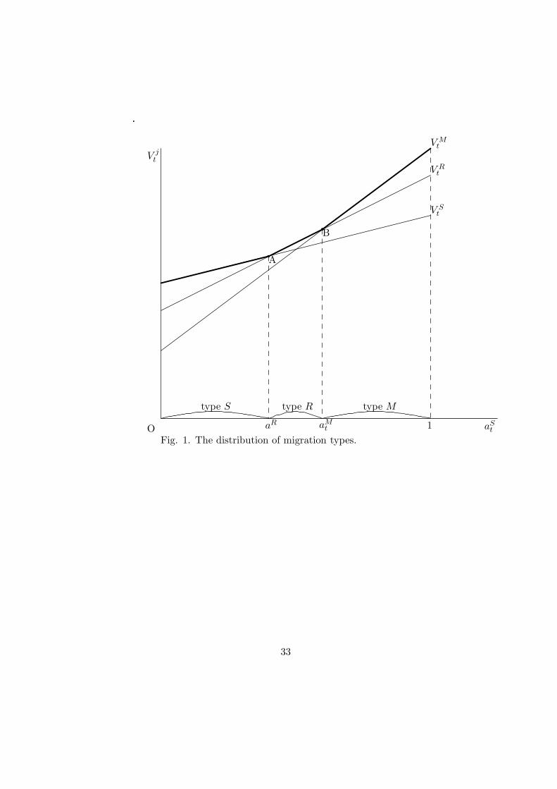
Fig. 1 illustrates the distribution of migration types under Assumption

3 in (aSt , V j

t ) plane. Curves V St , V R

t , and V Mt stand for Eqs. (23), (24),

and (25), respectively. The two cutoffs aR and aMt are determined at points

A and B, respectively. They partition the unit interval into three subsets,

[0, aR], [aR, aMt ], and [aM

t , 1]. First, households with low abilities aSt ∈ [0, aR]

stay home because their gains from studying or working abroad cannot cover

the fixed costs. Second, households with intermediate abilities aSt ∈ [aR, aM

t ]

study abroad but return home for work. Although their ability is sufficiently

high to cover the fixed cost of studying abroad, their gains from working

abroad are not as high as returning home. Third, households with aSt ∈

[aMt , 1] are able enough to study and work abroad. Thus, households with

different abilities are sorted into different migration types: the more able a

person is, the more likely she is to study and work abroad. The measures

of sets [0, aR], [aR, aMt ], and [aM

t , 1] are aR, aMt − aR, and 1 − aM

t , which

represent the fractions of types S,R, and M, respectively.

Proposition 1 says that the cutoff between types S and R is time-

invariant because changes in factor prices affect them equally as they both

work in their home country. However, since types R and M work in differ-

ent countries, the cutoff between them depends on different macroeconomic

conditions in the two countries, which in turn depend on the cutoff itself

through factor markets.

3.2 Markets

The market-clearing conditions for capital and effective labor in the two

countries are given by, respectively:

15

KSt =

∫ aR

0sSt−1(a

St−1)daS

t−1 +

∫ aMt−1

aR

sRt−1(a

St−1)daS

t−1, (29)

LSt =

∫ aR

0ES(aS

t )daSt +

∫ aMt

aR

(EN (aSt ) − f)daS

t , (30)

KNt =

∫ 1

0sNt−1(a

Nt−1)daN

t−1 +

∫ 1

aMt−1

sMt−1(a

St−1)daS

t−1, (31)

LNt =

∫ 1

0EN (aN

t )daNt +

∫ 1

aMt

(EN (aSt ) − f − g)daS

t , (32)

where the constancy of aR from Eq. (28) is considered. The world

market-clearing condition for the final good is omitted to save space. It

is important to note how different types of migrants contribute to factor

markets. Households of type M, the permanent migrants, supply effective

labor and capital in the host country. On the other hand, households of

type R, the return migrants, participate in factor markets in the source

country. From Eqs. (1), (2), (3), (7), (13), (14), (21), and (22), we can

derive Walras’ law. This implies that Eqs. (29), (30), (31), and (32) are

enough, whereas the world market-clearing condition for the final good is

redundant, to characterize an equilibrium.8

3.3 Dynamic system

From Eqs. (3), (4), (7), (14), (21), (22), (28), (29), (30), (31), and (32), we

obtain:

8In fact, as long as the factor market-clearing conditions are met, the demand for thefinal good is equal to its supply within each country. In other words, trade in the finalgood does not occur even if allowed. This is not surprising because there is only one finalgood.

16

kSt+1 = [(1 − α)BS/(2 + ρ)](kS

t )αLS(aR, aMt )/LS(aR, aM

t+1); (33)

LS(aR, aMt ) ≡

∫ aR

0ES(aS

t )daSt +

∫ aMt

aR

(EN (aSt ) − f)daS

t ,

kNt+1 = [(1 − α)BN/(2 + ρ)](kN

t )αLN (aMt )/LN (aM

t+1); (34)

LN (aMt ) ≡

∫ 1

0EN (aN

t )daNt +

∫ 1

aMt

(EN (aSt ) − f − g)daS

t .

Compared with Eq. (18), Eqs. (33) and (34) indicate that the evolution

of the capital/effective labor ratios is affected by migration. For example,

when aMt increases to aM

t+1, more households return to their home coun-

try (because aMt − aR increases), and so the capital/effective labor ratio in

country S decreases whereas that in country N increases in period t + 1.

Using Eqs. (13), (14), (20), (33), and (34), Eqs. (23), (24), and (25) are

rewritten as:

V St (aS

t ) = D + (2 + ρ + α) ln BS + (1 + ρ + α)α ln kSt + (2 + ρ) ln ES(aS

t )

+ (1 − α) ln(LS(aR, aMt+1)/L

S(aR, aMt )), (35)

V Rt (aS

t ) = D + (2 + ρ + α) ln BS + (1 + ρ + α)α ln kSt + (2 + ρ) ln(EN (aS

t ) − f)

+ (1 − α) ln(LS(aR, aMt+1)/L

S(aR, aMt )), (36)

V Mt (aS

t ) = D + (2 + ρ + α) ln BN + (1 + ρ + α)α ln kNt + (2 + ρ) ln(EN (aS

t ) − f − g)

+ (1 − α) ln(LN (aMt+1)/L

N (aMt )). (37)

The last terms in Eqs. (35), (36), and (37) reflect the aforementioned

demographic effects of migration on individual utility. A decrease in kSt+1

caused by an increase in aMt to aM

t+1, for example, raises country S’s rental

rate in period t + 1, which raises utility of types S and R of generation t.

In other words, an increase in a country’s working population is good for its

close older generation.

In deriving our dynamic system, let us define κt ≡ KSt /KN

t as the relative

17

supply of capital in country S to country N. Rewriting Eqs. (33) and (34)

to obtain the expressions for KSt+1 and KN

t+1, and dividing the former by the

latter, we have:

κt+1 = Bκαt λ(aR, aM

t )1−α;B ≡ BS/BN < 1, λ(aR, aMt ) ≡ LS(aR, aM

t )/LN (aMt ),

(38)

where λ(aR, aMt ) is the relative supply of effective labor in country S to

country N. Its partial derivatives are calculated as:

λR(aR, aMt ) ≡ ∂λ(aR, aM

t )/∂aR = [ES(aR) − (EN (aR) − f)]/LN (aMt ) = 0,

(39)

λM (aR, aMt ) ≡ ∂λ(aR, aM

t )/∂aMt

= [(EN (aMt ) − f)LN(aM

t ) + LS(aR, aMt )(EN (aM

t ) − f − g)]/LN (aMt )2 > 0.

(40)

An increase in aMt increases LS but decreases LN , both of which increase

λ. On the other hand, an increase in aR has no effect on λ because an increase

in LS by ES(aR) is exactly offset by a decrease in LS by EN (aR) − f.

Substituting Eqs. (36) and (37) into Eq. (27), we obtain:

0 = (2 + ρ + α) ln B + (1 + ρ + α)α(ln κt − ln λ(aR, aMt ))

+ (2 + ρ)(ln(EN (aMt ) − f) − ln(EN (aM

t ) − f − g))

+ (1 − α)(ln λ(aR, aMt+1) − ln λ(aR, aM

t )). (41)

The right-hand side of Eq. (41) is interpreted as the net benefit of

changing from a permanent migrant to a return migrant for a household of

generation t born in country S. The first and second terms represent costs

of returning home: country S is relatively less productive, and probably has

a lower capital/effective labor ratio, than country N.9 The third term shows

9Country S’s capital/effective labor ratio relative to country N is kSt /kN

t =

18

a benefit of returning home in that it saves the fixed cost of working abroad.

The fourth term captures the demographic effects of migration mentioned

above. It can be either positive or negative, depending on whether aMt+1

increases or decreases from aMt .

Eqs. (38) and (41), together with the initial condition κ0 = KS0 /KN

0 (>

0), constitute an autonomous system of two-dimensional first-order differ-

ence equations with respect to a state variable κt and a control variable aMt .

Once an equilibrium path {κt, aMt }∞t=0 is determined, all other endogenous

variables are determined as well.

3.4 Existence, uniqueness, and stability of a steady state

In a steady state, we have κt+1 = κt = κ and aMt+1 = aM

t = aM , where a

tilde over a variable represents a steady state under free migration. Then

Eq. (38) implies that κ is proportional to λ(aR, aM ):

κ = B1/(1−α)λ(aR, aM ). (42)

Substituting Eq. (42) into Eq. (41), and noting that 2 + ρ + α + (1 +

ρ + α)α[1/(1 − α)] = (2 + ρ)/(1 − α), aM is determined by:

(EN (aM ) − f)/(EN (aM ) − f − g) = B−1/(1−α) ⇒ aM = aM (f, g,B). (43)

Proposition 2 In the dynamic system consisting of Eqs. (38) and (41),

there exists a unique steady state (κ, aM ) such that aM ∈ (aR, 1) if:

(1 − B1/(1−α))(EN (aR) − f) < g < (1 − B1/(1−α))(EN (1) − f). (44)

Moreover, the dynamic system is saddle-path stable around the steady

state. During the transition, aMt moves in the same direction as κt.

Proof. From Proposition 1, there exists a unique aM ∈ (aR, 1) if the second

(KSt /LS

t )/(KNt /LN

t ) = κt/λ(aR, aMt ).

19

and third conditions of Assumption 3 hold in the steady state. From Eq.

(43), they are equivalent to (EN (aR) − f)/(EN (aR) − f − g) > B−1/(1−α)

and (EN (1) − f)/(EN (1) − f − g) < B−1/(1−α), respectively. Solving these

inequalities for g, we obtain Eq. (44).

On the other hand, κ is uniquely determined from Eq. (42) because

λ(aR, aM ) is monotonically increasing in aM from Eq. (40).

As for stability, linearizing Eqs. (38) and (41) around the steady state,

and using Eqs. (40), (42), and (43), we obtain:

[κt+1 − κ

aMt+1 − aM

]= J

[κt − κ

aMt − aM

]; (45)

J ≡

[j11 j12

j21 j22

],

j11 ≡ α ∈ (0, 1),

j12 ≡ (1 − α)κλM/λ > 0,

j21 ≡ −(1/∆)(1 + ρ + α)α/κ < 0,

j22 ≡ (1/∆){∆ + (1 + ρ + α)αλM /λ + (2 + ρ)ENa g/[(EN − f)(EN − f − g)]} > 1,

∆ ≡ (1 − α)λM/λ > 0.

In Appendix A, we show that the characteristic equation associated with

the Jacobian matrix J of Eq. (45) with one state variable and one control

variable has two eigenvalues with 0 < λ1 < 1 < λ2, and thus the dynamic

system is saddle-path stable. Finally, it is verified in Appendix A that the

stable arm is upward-sloping in the (κt, aMt ) plane, meaning that κt and aM

t

move in the same direction during the transition.

Fig. 2 describes the equilibrium path in the (κt, aMt ) plane. Appendix

A verifies that both the κt+1 = κt and aMt+1 = aM

t loci are upward-sloping,

and that the former is steeper than the latter. We have κt+1 > κt above the

κt+1 = κt locus, whereas κt+1 < κt below it. As more people return home

(i.e., aMt increases), country S becomes relatively more populated, and so it

accumulates capital more relatively to the next period. On the other hand,

20

aMt+1 < aM

t to the right of the aMt+1 = aM

t locus, whereas aMt+1 > aM

t to

the left of it. This is because an increase in κt increases the net benefit of

returning home, which should be compensated for by a decrease in country

S’s working population for the next period. The steady state is found at

point B, the intersection of the κt+1 = κt and aMt+1 = aM

t loci. The stable

arm, drawn by arrows toward point B, is upward-sloping but flatter than

the aMt+1 = aM

t locus.

Proposition 2 has interesting implications. Suppose that country S is

initially poor in capital stock: κ0 < κ in Figure 1. Then aM0 is found at

point A on the stable arm. After that, the equilibrium point moves to the

northeast along the stable arm until it reaches point B. As capital gradually

accumulates in country S, more and more students choose to return home

after finishing their studies in country N . This matches the fact that a lot

more Chinese and Indian students are returning to their respective home

countries in recent years, while 20 some years ago few of them did that.

4 Comparative dynamics

Having shown that our model exhibits well-behaved dynamics, we next ex-

amine the effects of exogenous shocks on some endogenous variables. We are

particularly interested in changes in the fixed costs of studying and working

abroad because they will directly affect the distribution of migration types.

4.1 A decrease in the fixed cost of studying abroad

Totally differentiating Eqs. (38) and (41) with df 6= 0, and using Eqs. (39),

(40), (42), and (43), we have:

[dκt+1

daMt+1

]= J

[dκt

daMt

]+

[0

−(1/∆)(2 + ρ)g/[(EN − f)(EN − f − g)]

]df.

Letting κt+1 = κt = κ and aMt+1 = aM

t = aM , we obtain:

21

∂κ/∂f = −(1/ϕ(1))j12(1/∆)(2 + ρ)g/[(EN − f)(EN − f − g)] > 0,

∂aM/∂f = −(1/ϕ(1)){−(j11 − 1)(1/∆)(2 + ρ)g/[(EN − f)(EN − f − g)]} > 0,

where ϕ(λ) is the characteristic polynomial associated with J, and ϕ(1) <

0.

In Fig. 3, suppose that we are originally at point B, the old steady

state. A decrease in f shifts the aMt+1 = aM

t locus down to (aMt+1 = aM

t )′,

but leaves the κt+1 = κt locus unchanged. The new steady state moves to

point D, which is to the southwest of point B on the κt+1 = κt locus. The

new stable arm is drawn by arrows toward point D. In the initial period, the

equilibrium point jumps down from point B to point C on the new stable

arm. Then the equilibrium point gradually moves to the southwest along

the new stable arm to point D. As a result, both aM and κ decrease.

The above adjustment process can be interpreted as follows. In period

0, a decrease in f increases the effective labor of both types R and M

by the same amount. Then the utility of type M with a smaller effective

labor increases more than type R due to diminishing marginal utility. This

induces some type R whose ability was close to aM in the old steady state to

switch to type M. Since the working population of country S decreases due

to the increase in the fraction of permanent migrants, the relative supply

of capital in country S to country N decreases for the next period. In

period 1, the decrease in κ1 reduces the utility of type R relative to type M,

which further decreases aM1 and hence κ2. This process continues until the

equilibrium point reaches point D.

Although the fraction of permanent migrants 1−aM surely increases with

a decrease in f, it is unclear how the fraction of return migrants aM − aR

changes because aR also decreases from Proposition 1. More specifically,

Eqs. (12) and (28) imply that:

daR/df = 1/(ENa − ES

a ) > 0.

22

A decrease in f increases aM − aR if and only if ∂aM/∂f − daR/df < 0,

or daR/df > ∂aM/∂f > 0. This is more likely, the smaller is the difference

between the slopes of EN (aSt ) and ES(aS

t ). Our results are summarized in

the following proposition:

Proposition 3 In the steady state, a permanent decrease in the fixed cost of

studying abroad: (i) decreases the fraction of non-migrants aR; (ii) increases

the fraction of return migrants aM − aR if ENa − ES

a is sufficiently small;

(iii) increases the fraction of permanent migrants 1− aM ; and (iv) decreases

the relative supply of capital in the source country κ.

Example If the acquired effective labor function is specified as hi(eit, a

it) =

H ieait(ei

t)γ ; 0 < HS < HN , γ ∈ (0, 1), where e is Euler’s number (i.e., the

base of the natural logarithm), then we obtain daR/df = (1 − γ)/f and

∂aM/∂f = (1 − γ)/[(1 − B1/(1−α))−1g − 1 + f ]. Since (1 − B1/(1−α))−1g >

EN (aR)−f from Eq. (44), and EN (aR)−f = 1+[(HS)1/(1−γ)/((HN )1/(1−γ)−

(HS)1/(1−γ))]f > 1, we have daR/df > ∂aM/∂f. Therefore, a decrease in f

increases aM − aR under this specification.

4.2 A decrease in the fixed cost of working abroad

In the same way as the previous case, we can show that:

∂κ/∂g = −(1/ϕ(1))j12(1/∆)(2 + ρ)/(EN − f − g) > 0,

∂aM/∂g = −(1/ϕ(1))[−(j11 − 1)(1/∆)(2 + ρ)/(EN − f − g)] > 0.

Since aR is independent of g, we immediately obtain the following propo-

sition:

Proposition 4 In the steady state, a permanent decrease in the fixed cost

of working abroad: (i) leaves the fraction of non-migrants aR unchanged;

(ii) decreases the fraction of return migrants aM − aR; (iii) increases the

fraction of permanent migrants 1− aM ; and (iv) decreases the relative supply

of capital in the source country κ.

23

A dynamic implication of Propositions 4 and 5 is that facilitating either

studying or working abroad discourages capital accumulation in the source

country. This is simply because capital is supplied from the savings of the

working population of the old generation. As more people decide to work

abroad, the source country has less workers. Then they save less in the

aggregate even if the return migrants save more. We next consider how we

can encourage studying abroad without discouraging capital accumulation.

4.3 Offsetting changes in the fixed costs of studying and

working abroad

Suppose that a decrease in the fixed cost of studying abroad is combined

with an offsetting increase in the fixed cost of working abroad: df < 0, dg =

−df > 0. From the results in sections 4.1 and 4.2, we immediately obtain:

dκ/df |dg=−df = ∂κ/∂f − ∂κ/∂g

= −(1/ϕ(1))j12(1/∆)(2 + ρ)[−1/(EN − f)] < 0,

daM/df |dg=−df = ∂aM/∂f − ∂aM/∂g

= −(1/ϕ(1)){−(j11 − 1)(1/∆)(2 + ρ)[−1/(EN − f)]} < 0.

Remembering the fact that aR is increasing in f but independent of g,

we reach the following proposition:

Proposition 5 In the steady state, a permanent decrease in the fixed cost

of studying abroad and an offsetting permanent increase in the fixed cost of

working abroad: (i) decrease the fraction of non-migrants aR; (ii) increase

the fraction of return migrants aM − aR; (iii) decrease the fraction of per-

manent migrants 1 − aM ; and (iv) increase the relative supply of capital in

the source country κ.

In view of Eq. (41), a decrease in f and an offsetting increase in g raises

the net benefit of returning home. This induces some of the permanent

migrants to return to their home country. Moreover, from Eq. (38), the

24

increased working population in the source country increases its relative

supply of capital for the next period, which further makes returning home

more desirable. Thus, we can promote studying abroad and returning home

at the same time, which helps the source country turn “brain drain” into

“brain gain”.

4.4 Individual utility in the steady state

From Eqs. (20), (35), (36), and (37), individual utility in the steady state

is expressed as:

V S(aSt ) = D + (2 + ρ + α) ln BS + (1 + ρ + α)α ln kS + (2 + ρ) ln ES(aS

t ),

V R(aSt ) = D + (2 + ρ + α) ln BS + (1 + ρ + α)α ln kS + (2 + ρ) ln(EN (aS

t ) − f),

V M (aSt ) = D + (2 + ρ + α) ln BN + (1 + ρ + α)α ln kN + (2 + ρ) ln(EN (aS

t ) − f − g),

V N (aNt ) = D + (2 + ρ + α) ln BN + (1 + ρ + α)α ln kN + (2 + ρ) ln EN (aN

t ).

Comparing Eqs. (33) and (34) with Eq. (19), each country’s capi-

tal/effective labor ratio in the steady state under free migration is the same

as that under autarky, and is independent of f and g:

kS = [(1 − α)BS/(2 + ρ)]1/(1−α) = kS,

kN = [(1 − α)BN/(2 + ρ)]1/(1−α) = kN

.

We first consider a decrease in the fixed cost of studying abroad from f

to f ′(< f). Then both aR and aM decrease to aR′(< aR) and aM ′(< aM ),

respectively. It is clear that the utility of all households born in country N

is unchanged in the steady state. On the other hand, the individual utility

of households born in country S can be examined in Fig. 4. Suppose that

the utility of types S,R, and M in the old steady state are given by curves

V S, V R, and V M , respectively. Point A, the intersection of curves V S and

V R, determines aR. On the other hand, curves V R and V M intersect at

25

point B, which gives aM . A decrease in f shifts both curves V R and V M up

to curves V R′ and V M ′, respectively. Both points A and B move leftward to

points C and D, respectively. In the illustrated case, the fractions of both

permanent and return migrants increase. There emerge five groups who

are differently affected by a decrease in f : (i) V S′(aSt ) = V S(aS

t ) for aSt ∈

[0, aR′]; (ii) V R′(aSt ) > V S(aS

t ) for aSt ∈ [aR′, aR]; (iii) V R′(aS

t ) > V R(aSt )

for aSt ∈ [aR, aM ′]; (iv) V M ′(aS

t ) > V R(aSt ) for aS

t ∈ [aM ′, aM ]; and (v)

V M ′(aSt ) > V M (aS

t ) for aSt ∈ [aM , 1]. Groups (iii) and (v) gain simply by

supplying more effective labor. On the other hand, groups (ii) and (iv) gain

from changes in migration status. Overall, a decrease in the fixed cost of

studying abroad does no harm to anyone in the steady state.

The effect of a decrease in the fixed cost of working abroad on individual

utility can be examined similarly. When g decreases to g′′(< g), only aM

decreases to aM ′′(< aM ). The utility of type M increases, whereas that of

the rest is unchanged.

Finally, a decrease in the fixed cost of studying abroad and an offsetting

increase in the fixed cost of working abroad shifts only curve V R up. This

widens the range of ability for return migrants to both sides, and their

utility increases as a result. Since the amount of increase in g is limited to

the amount of decrease in f, the utility is unchanged for both permanent

migrants and non-migrants.

Proposition 6 In the steady state:

1. a permanent decrease in the fixed cost of studying abroad increases

the utility of all permanent and return migrants, whereas it leaves the

utility of all non-migrants unchanged;

2. a permanent decrease in the fixed cost of working abroad increases the

utility of all permanent migrants, whereas it leaves the utility of all

return migrants and non-migrants unchanged;

3. a permanent decrease in the fixed cost of studying abroad and an off-

setting permanent increase in the fixed cost of working abroad increase

26

the utility of all return migrants, whereas they leave the utility of all

permanent migrants and non-migrants unchanged.

Considering Propositions 3 to 6, the third option has an advantage over

the first and second ones. Any single change in either f or g causes a tradeoff

between the utility of some migrant groups and the relative supply of capital

in the source country. For example, a single increase in g increases κ but

decreases the utility of type M. Oh the other hand, a combined decrease

in f and an offsetting increase in g are free from such a tradeoff: they

increase both κ and the utility of type R without hurting anyone else. If the

government in the source country cares about growth as well as welfare, the

third option is the best.

5 Concluding remarks

Our analysis based on a two-country dynamic general equilibrium model

has some implications for growth-enhancing migration policies. First, dis-

couraging either studying or working abroad enables the source country to

accumulate more capital, but at the expense of permanent migrants and pos-

sibly return migrants. For example, a well-known brain drain tax proposed

by Bhagwati and Hamada (1974), which can be interpreted as an increase

in g in the present model, harms permanent emigrants. Second, however,

offsetting changes in the fixed costs of studying and working abroad can be

both growth-enhancing for the source country and Pareto-improving for the

world. This may provide policy guidance for developing countries trying to

encourage students studying abroad to return home and help develop their

motherland countries.

It is considerable that returning home may require some cost. In our

model, incorporating such a cost for return migration can create an addi-

tional cutoff, such that those students with the lowest abilities may not be

able to pay this cost and return home. As a consequence, they could end up

working illegally in the host countries after their student visas expire. Then,

the students studying abroad can be divided into three groups: those with

27

highest ability stay permanently with good jobs in the host country, those

with middle ability choose to return home, and those with lowest ability

stay illegally.

Two other possible extensions are also interesting. First, the migration

costs in the model can be considered as caused by changes in taxes or sub-

sidies. Then it would become realistic to design an appropriate tax-subsidy

scheme under the government budget constraint. Second, our analysis is still

limited to a neoclassical growth model with no growth in the steady state. It

will be interesting to include endogenous growth, whether accumulation- or

R&D-based, and see how migration patterns interact with long-run growth.

Appendix A. Transitional dynamics

The characteristic equation associated with the Jacobian matrix J of Eq.

(45) is:

ϕ(λ) ≡ det(λI−J) =

∣∣∣∣∣λ − j11 −j12

−j21 λ − j22

∣∣∣∣∣ = λ2−(j11+j22)λ+j11j22−j12j21.

Since j11 + j22 > 0 and j11j22 − j12j21 > 0, both eigenvalues satisfying

that ϕ(λ) = 0 have positive real parts. Let λ1 and λ2 be the two eigenvalues

such that 0 < λ1 < λ2. Moreover, evaluating ϕ(λ) at λ = 1, we have:

ϕ(1) = 1 − (j11 + j22) + j11j22 − j12j21

= −(1/∆)(1 − α)(2 + ρ)ENa g/[(EN − f)(EN − f − g)] < 0.

This implies that 0 < λ1 < 1 < λ2, ensuring saddle-path stability.

We next derive the stable arm representing the equilibrium path. The

eigenvectors associated with λ1 and λ2 are given by v1 ≡ [1, j21/(λ1 − j22)]T

and v2 ≡ [1, j21/(λ2 − j22)]T , respectively. With V ≡ [v1, v2], let us define

two transformed variables xt and yt such that:

28

[κt − κ

aMt − aM

]≡ V

[xt

yt

].

Then, since Eq. (45) is rewritten as:

[xt+1

yt+1

]= V −1JV

[xt

yt

]=

[λ1 0

0 λ2

][xt

yt

],

xt and yt are solved as, respectively:

xt = λt1x0,

yt = λt2y0.

Transforming them back, we obtain:

κt − κ = λt1x0 + λt

2y0,

aMt − aM = [j21/(λ1 − j22)]λ

t1x0 + [j21/(λ2 − j22)]λ

t2y0.

Since λ2 > 1, we must have y0 = 0 for the dynamic system not to

explode. Therefore, it is reduced to:

κt − κ = λt1x0,

aMt − aM = [j21/(λ1 − j22)]λ

t1x0.

Since κ0 − κ = x0 in the initial period, we finally obtain:

κt − κ = λt1(κ0 − κ),

aMt − aM = [j21/(λ1 − j22)]λ

t1(κ0 − κ) = [j21/(λ1 − j22)](κt − κ).

The last equation shows the stable arm. Its slope in the (κt, aMt ) plane

29

is given by:

(aMt − aM )/(κt − κ)|SA = j21/(λ1 − j22) > 0.

On the other hand, from Eq. (45), the slopes of the κt+1 = κt and

aMt+1 = aM

t loci are calculated as, respectively:

(aMt − aM )/(κt − κ)|κt+1=κt

= −(j11 − 1)/j12 > 0,

(aMt − aM )/(κt − κ)|aM

t+1=aM

t= −j21/(j22 − 1) > 0.

It turns out that the κt+1 = κt locus is steeper than the aMt+1 = aM

t

locus:

(aMt −aM)/(κt−κ)|κt+1=κt

−(aMt −aM)/(κt−κ)|aM

t+1=aM

t= −ϕ(1)/[j12(j22−1)] > 0.

We can also see that the stable arm is flatter than the aMt+1 = aM

t locus:

(aMt −aM)/(κt−κ)|aM

t+1=aM

t−(aM

t −aM )/(κt−κ)|SA = j21(−1+λ1)/[(j22−λ1)(j22−1)] > 0.

30

References

[1] Bhagwati, J., Hamada, K., 1974. The drain drain, international inte-

gration of markets for professionals and unemployment: a theoretical

analysis. Journal of Development Economics 1, 19–42.

[2] Borjas, G. J., Bratsberg, B., 1996. Who leaves? the outmigration of

the foreign-born. Review of Economics and Statistics 78, 165–176.

[3] Chacko, E., 2007. From brain drain to brain gain: reverse migration

to Bangalore and Hyderabad, India’s globalizing high tech cities. Geo-

Journal 68, 131–140.

[4] Djajic, S., 2008. Immigrant parents and children: an analysis of deci-

sions related to return migration. Review of Development Economics

12, 469–485.

[5] Domingues Dos Santos, M., Postel-Vinay, F., 2003. Migration as a

source of growth: the perspective of a developing country. Journal of

Population Economics 16, 161–175.

[6] Dustmann, C., 1997. Return migration, uncertainty and precautionary

savings. Journal of Development Economics 52, 295–316.

[7] Dustmann, C., 2003. Children and return migration. Journal of Popu-

lation Economics 16, 815–830.

[8] Dustmann, C., Fadlon, I., Weiss, Y., 2011. Return migration, human

capital accumulation and the brain drain. Journal of Development Eco-

nomics 95, 58–67.

[9] Fujishima, S., 2013. Growth, agglomeration, and urban congestion.

Journal of Economic Dynamics and Control 37, 1168–1181.

[10] Galor, O., Stark, O., 1990. Migrants’ savings, the probability of return

migration and migrants’ performance. International Economic Review

31, 463–467.

31

[11] Ivanova, V., 2013. Return migration: existing policies and practices in

Bulgaria, in: Zwania-Roessler, I., Ivanova, V. (Eds.), Welcome Home?

Challenges and Chances of Return Migration. German Marshall Fund

of the United States, Washington, DC, pp. 8-18.

<http://www.gmfus.org/wp-content/blogs.dir/1/files mf/1358538301tfmireturnmigration.pdf>,

last accessed February 27, 2014.

[12] Lange, T., 2013. Return migration of foreign students and non-resident

tuition fees. Journal of Population Economics 26, 703–718.

[13] MATT, 2013. The US/Mexico cycle: end of an era.

<http://www.matt.org/uploads/2/4/9/3/24932918/returnmigration top line www.pdf>,

last accessed February 27, 2014.

[14] Zweig, D., 2006. Competing for talent: China’s strategies to reverse the

brain drain. International Labour Review 145, 65–90.

32

OFig. 1. The distribution of migration types.

aSt

V jt

V St

V Rt

V Mt

aR aMt

A

B

1

type S type R type M

33

OFig. 2. The equilibrium path: κ0 < κ.

κt

aMt

κ

aM B

κ0

aM0

aMt+1 = aM

tκt+1 = κt

A

aR

34

OFig. 3. The effect of a decrease in f on the equilibrium path.

κt

aMt

κ

aM B

(aMt+1 = aM

t )′

κt+1 = κt

D

C

κ′

aM ′

aM ′0

aR

35

OFig. 4. The effect of a decrease in f on individual utility in the steady state.

aSt

V j

V S

V R

V M

aR aM

A

B

1

V R′

V M ′

C

D

aR′ aM ′

36


Recommended