Capital Budgeting Techniques and Real Option

Quantitative Methods in

Capital Budgeting & Real Options Techniques

Thesis submitted for the degree of Master of Science in

Management of Business, Innovation & Technology

Supervisor: Prof. Gregory S. Yovanof

By

Pantazis Houlis

March 2009

Quantitative Methods in Capital Budgeting and Real Options Techniques 2

Abstract

Capital budgeting is the decision process that managers use to identify those projects that add to the firm’s value. A firm’s capital budgeting decisions define its strategic direction. Its growth, as well as its ability to sustain a competitive advantage depend upon a constant flow of ideas for new products and services, for ways of making existing products better and for ways to operate at a lower cost. Capital budgeting is the process of evaluating specific investment decisions. These are the decisions that determine a firm’s competitive success in a changing technological and competitive landscape.

Several quantitative techniques have been developed to help rank projects and to decide whether they should be accepted for implementation. These techniques are analysed in the prism of evaluating a new product development project.

Traditional valuation approaches such as Payback period, NPV, IRR are first addressed with the Discounted Cash Flow model. Subsequently, sensitivity and scenario analysis are applied followed by Monte Carlo Simulation and Decision Tree techniques.

Having discussed the limitations of the traditional approaches, Real Options analysis is addressed, taking into account the value of uncertainty in strategic investment decision making. The methodologies employed include closed form models, the binomial lattice method and a stochastic simulation technique utilising a Geometric Brownian Motion model.

This framework of capital investment decision making tools is applied to a specific business case, involving a new venture developing a product in the consumer electronics market. With the help of these tools a thorough examination is performed, providing insights into the attractiveness of this business opportunity.


Table of Contents

1. Introduction................................................................................... 4 1.2 Research Problem and Objectives ............................................ 5 1.3 Project Classifications .............................................................. 5 1.4 The Capital Budgeting Process ................................................. 6

2. Case Study Description .................................................................. 8 2.1 “WebPulse” Project .................................................................. 8 2.2 Project Model............................................................................ 9

3. Traditional Valuation Methods..................................................... 13 3.1 Payback Period ....................................................................... 13 3.2 Discounted Cash Flow (DCF) - Net Present Value (NPV) ........ 14 3.3 Internal Rate of Return (IRR) ................................................ 16 3.4 Modified Internal Rate of Return (MIRR)............................... 16 3.5 Profitability Index (PI) ........................................................... 17

4. Risk Analysis Techniques ............................................................. 18 4.1 Sensitivity Analysis................................................................. 18 4.2 Scenario Analysis.................................................................... 20 4.3 Monte Carlo Simulation .......................................................... 21 4.4 Decision Tree Analysis ............................................................ 33

5. Real Options ................................................................................ 35 5.1 Real Options Valuation Approach ........................................... 37 5.2 Timing Option - Decision Tree Method ................................... 38 5.3 Timing Option - Black Scholes Model...................................... 39 5.3 Binomial Lattice – Growth & Abandonment Option................ 42 5.4 Geometric Brownian Motion Simulation Model ...................... 48

6. Conclusions.................................................................................. 51

References ....................................................................................... 54

Appendix.......................................................................................... 55 A.1 Time Value of Money .............................................................. 55 A.2 Estimation of Volatility – Logarithmic Cash Flow Returns Approach ...................................................................................... 56


1. Introduction

Financial management is largely concerned with financing, dividend and investment decisions of the firm. The most widely accepted objective for the firm is to maximize the value of the firm to its owners.

Financing decisions deal with the firm’s optimal capital structure in terms of debt and equity. Dividend decisions relate to the form in which returns generated by the firm are passed on to equity-holders. Investment decisions deal with the way funds raised in financial markets are employed in productive activities to achieve the firm’s overall goal; in other words, how much should be invested and what assets should be invested in. The relationship between the firm’s overall goal, financial management and capital budgeting is depicted in Figure 1.1.

Figure 1.1 Corporate goal, financial management and capital budgeting.

Funds are invested in both short-term and long-term assets. Capital budgeting is primarily concerned with sizable investments in log-term assets. These assets may be tangible items such as property, plant or equipment or intangible ones such as new technology, patents or trademarks. Investments in processes such as research, design, development and testing, through which new technology and new products are created, may also be viewed as investments in intangible assets.

Irrespective of whether the investments are in tangible or intangible assets, a capital investment project can be distinguished from recurrent expenditures by two features. One is that such projects are significantly large. The other is that they are generally long-lived projects with their benefits or cash flows spreading over many years.

Sizable, long-term investments in tangible or intangible assets have long-term consequences. An investment today will determine the firm’s strategic position many years hence. These investments also have a considerable impact on the

Goal of the Firm Maximize shareholder wealth or value of the firm

Financing Decision

Investment Decision

Dividend Decision

Short-term Investments

Long-term Investments

Capital Budgeting


organization’s future cash flows and the risk associated with those cash flows. Capital budgeting decisions thus have a long-range impact on the firm’s performance and they are critical to the firm’s success or failure.

1.2 Research Problem and Objectives

The aim of this thesis is to provide an overview of quantitative methods used to assist in strategic investment decision making. How can one choose between several projects? What is the value of a proposed new business endeavour? What are the chances the invested amount will produce multiple returns? Will the capital invested be recouped and when? These are but only of few of the questions managers are faced with when planning their firm’s strategy.

The use and mechanics behind these techniques are illustrated through their application in a new product development project – the “WebPulse” case study, where their strengths and limitations are analysed. Opportunities created from uncertainty are revealed using a real options approach. Finally, a methodology framework is provided, covering both traditional techniques and the more recent real options methods.

1.3 Project Classifications

Analysing capital expenditure proposals is not a costless operation. For certain types of projects, a relatively detailed analysis may be warranted, while for others, simpler procedures should be used. Firms generally categorize projects and analyse them accordingly:

1. Replacement: maintenance of business. Replacement of worn-out or damaged equipment is necessary if the firm is to continue in business. The only issues here are (a) should this operation be continued and (b) should we continue to use the same production processes? If the answers are yes, maintenance decisions are normally made without an elaborate decision process.

2. Replacement: cost reduction. These projects lower the costs of labour, materials, and other inputs such as electricity by replacing serviceable but less efficient equipment. These decisions are discretionary and require a detailed analysis.

3. Expansion of existing products or markets. Expenditures to increase output of existing products, or to expand retail outlets or distribution facilities in markets now being served, are included here. These decisions are more complex because they require an explicit forecast of growth in demand, so a more detailed analysis is required. Also, the final decision is generally made at a higher level within the firm.

4. Expansion into new products or markets. These projects involve strategic decisions that could change the fundamental nature of the business, and they normally require the expenditure of large sums with delayed paybacks. Invariably, a detailed analysis is required, and the final decision is generally made at the very top – by the board of directors as a part of the firm’s strategic plan.


5. Safety and /or environmental projects. Expenditures necessary to comply with government orders, labour agreements, or insurance policy terms are called mandatory investments, and they often involve non-revenue-producing projects. How they are handled depends on their size, with small ones being treated much like the Category 1 projects described above.

6. Research and development. The expected cash flows from R&D are often too uncertain to warrant a standard discounted cash flow (DCF) analysis. Instead, decision tree analysis and the real options approach are often used.

7. Long-term contracts. Companies often make long-term contractual arrangements to provide products or services to specific customers. There may or may not be much up-front investment, but costs and revenues will accrue over multiple years, and a DCF analysis should be performed before the contract is signed.

1.4 The Capital Budgeting Process

Capital budgeting is a multi-faceted activity. There are several sequential stages in the process. For typical investment proposals of a large organisation, the distinctive stages in the capital budgeting process are depicted in the form of a simplified flow chart in Figure 1.2., where the shaded box underpins the focus of this thesis and its relation to the whole process.


Figure 1.2 The Capital Budgeting Process

Corporate goal

Strategic planning

Investment opportunities

Preliminary screening

Financial appraisal, quantitative analysis, Project evaluation or project analysis

Qualitative factor, judgments and gut feelings

Accept/reject decisions on the projects

Accept Reject

Implementation

Facilitation, monitoring, control and review

Continue, expand or abandon project

Post-implementation audit


2. Case Study Description

A new product development project was chosen in order to illustrate the advantages and limitations of each project valuation technique.

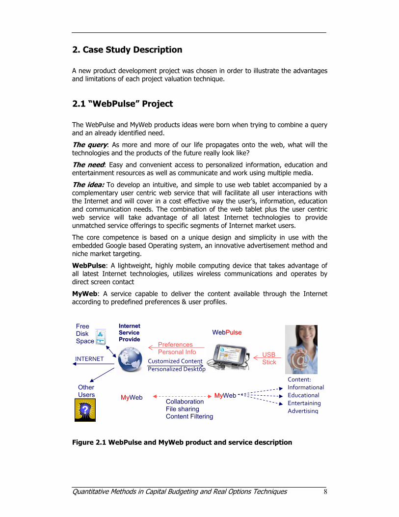
2.1 “WebPulse” Project

The WebPulse and MyWeb products ideas were born when trying to combine a query and an already identified need.

The query: As more and more of our life propagates onto the web, what will the technologies and the products of the future really look like?

The need: Easy and convenient access to personalized information, education and entertainment resources as well as communicate and work using multiple media.

The idea: To develop an intuitive, and simple to use web tablet accompanied by a complementary user centric web service that will facilitate all user interactions with the Internet and will cover in a cost effective way the user’s, information, education and communication needs. The combination of the web tablet plus the user centric web service will take advantage of all latest Internet technologies to provide unmatched service offerings to specific segments of Internet market users.

The core competence is based on a unique design and simplicity in use with the embedded Google based Operating system, an innovative advertisement method and niche market targeting.

WebPulse: A lightweight, highly mobile computing device that takes advantage of all latest Internet technologies, utilizes wireless communications and operates by direct screen contact

MyWeb: A service capable to deliver the content available through the Internet according to predefined preferences & user profiles.

Figure 2.1 WebPulse and MyWeb product and service description

IInntteerrnneett SSeerrvviiccee PPrroovviiddee

WWeebbPPuullssee

MMyyWebMMyyWeb

Content: Informational Educational Entertaining Advertising

Preferences Personal Info USB

StickCustomized Content Personalized Desktop

INTERNET

Free Disk Space

Other Users

Collaboration File sharing Content Filtering


2.2 Project Model

The prerequisite for quantitative valuation analysis of a project is it’s estimation of future cash flows. Free cash flow is calculated as follows:

Free Cash Flow = Net operating profit after taxes (NOPAT) + Depreciation - Gross fixed asset expenditures - Change in net operating working capital = EBIT (1 – T) + Depreciation - Gross fixed asset expenditures - [∆ Operating current assets – ∆ Operating current liabilities] Typically, cash flow estimation includes the following items:

1. Initial investment outlay. This includes the cost of the fixed assets associated with the project plus any initial investment in net operating working capital (NOWC), such as raw material.

2. Annual project cash flow. The operating cash flow is the net operating profit after taxes (NOPAT) plus depreciation. Depreciation is added back because it is a noncash expense and also because financing costs (including interest expenses) are not subtracted since they are accounted for when the cash flow is discounted at the cost of capital. In addition, many projects have levels of NOWC that change during the project’s life.

3. Terminal year cash flow. At the end of the project’s life, some extra cash flow is usually generated from the salvage value of the fixed assets, adjusted for taxes if the assets are not sold at their book value. Any return of net operating working capital not already accounted for in the annual cash flow should also be added in the terminal year cash flow.

For the WebPulse project it is estimated that annual sales would be 38.000 units if the units were priced at $400 each. It is expected that the unit price will not rise, while the annual growth in sales will be 15%. It is estimated that the fixed costs during the year 1 development phase are $500.000. The workspace required for development and manufacturing will be acquired by buying an existing building for $7.000.000, while the necessary equipment would be purchased for the amount of $3.000.000. The building will fall under the Modified Accelerated Cost Recovery System (MARCS) 39-year class, while the equipment would fall into the MARCS 5-year class.

The projects estimated economic life is four years. At the end of that time, the building is expected to have a market value of $5.950.000, whereas the equipment will have a market value of $900.000.

Variable manufacturing costs are estimated to be $280 per unit, and fixed overhead costs, excluding depreciation, will be $800.000 per year. It is expected that these costs will rise by 2% each year. It is also assumed that an amount of NOWC on hand equal to 10% of the upcoming year’s sales is necessary. The tax rate is 40% while the company’s cost of capital is 12%.


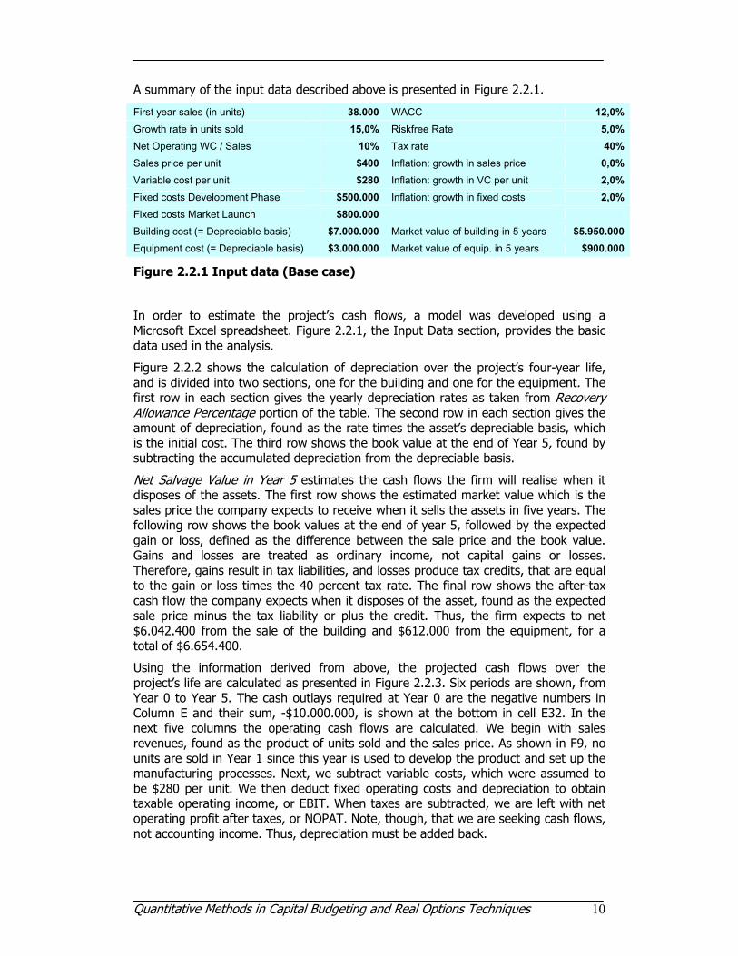
A summary of the input data described above is presented in Figure 2.2.1.

First year sales (in units) 38.000 WACC 12,0% Growth rate in units sold 15,0% Riskfree Rate 5,0% Net Operating WC / Sales 10% Tax rate 40% Sales price per unit $400 Inflation: growth in sales price 0,0% Variable cost per unit $280 Inflation: growth in VC per unit 2,0% Fixed costs Development Phase $500.000 Inflation: growth in fixed costs 2,0% Fixed costs Market Launch $800.000

Building cost (= Depreciable basis) $7.000.000 Market value of building in 5 years $5.950.000 Equipment cost (= Depreciable basis) $3.000.000 Market value of equip. in 5 years $900.000

Figure 2.2.1 Input data (Base case)

In order to estimate the project’s cash flows, a model was developed using a Microsoft Excel spreadsheet. Figure 2.2.1, the Input Data section, provides the basic data used in the analysis.

Figure 2.2.2 shows the calculation of depreciation over the project’s four-year life, and is divided into two sections, one for the building and one for the equipment. The first row in each section gives the yearly depreciation rates as taken from Recovery Allowance Percentage portion of the table. The second row in each section gives the amount of depreciation, found as the rate times the asset’s depreciable basis, which is the initial cost. The third row shows the book value at the end of Year 5, found by subtracting the accumulated depreciation from the depreciable basis.

Net Salvage Value in Year 5 estimates the cash flows the firm will realise when it disposes of the assets. The first row shows the estimated market value which is the sales price the company expects to receive when it sells the assets in five years. The following row shows the book values at the end of year 5, followed by the expected gain or loss, defined as the difference between the sale price and the book value. Gains and losses are treated as ordinary income, not capital gains or losses. Therefore, gains result in tax liabilities, and losses produce tax credits, that are equal to the gain or loss times the 40 percent tax rate. The final row shows the after-tax cash flow the company expects when it disposes of the asset, found as the expected sale price minus the tax liability or plus the credit. Thus, the firm expects to net $6.042.400 from the sale of the building and $612.000 from the equipment, for a total of $6.654.400.

Using the information derived from above, the projected cash flows over the project’s life are calculated as presented in Figure 2.2.3. Six periods are shown, from Year 0 to Year 5. The cash outlays required at Year 0 are the negative numbers in Column E and their sum, -$10.000.000, is shown at the bottom in cell E32. In the next five columns the operating cash flows are calculated. We begin with sales revenues, found as the product of units sold and the sales price. As shown in F9, no units are sold in Year 1 since this year is used to develop the product and set up the manufacturing processes. Next, we subtract variable costs, which were assumed to be $280 per unit. We then deduct fixed operating costs and depreciation to obtain taxable operating income, or EBIT. When taxes are subtracted, we are left with net operating profit after taxes, or NOPAT. Note, though, that we are seeking cash flows, not accounting income. Thus, depreciation must be added back.


Raw materials must be purchased and replenished each year as they are used. It is assumed that an amount of net operating working capital (NOWC) equal to 10% of

Figure 2.2.2 Depreciation and Net Salvage Value Estimations

the upcoming year’s sales is needed. Sales in Year 2 are $15.200.000, an amount of $1.520.000 is needed in Year 1 as NOWC as shown in cell F24. Since no NOWC existed for this project prior to Year 1, an investment of $1.520.000 must be made in Year 1 as shown in cell F25. Sales increase to $17.480.000 in Year 3, so $1.740.000 of NOWC is needed in Year 2. Since $1.520.000 already exist for this purpose, the net investment would only be $228.000 in Year 2 as shown in cell G25. Note that there are no sales after Year 5, so no NOWC is required in Year 5. Thus, there is a positive cash flow of $2.010.200 at Year 5 as working capital is sold but not replaced.

When the project’s life ends, the company will receive the “Salvage Cash Flows” as shown in the column for Year 5 in the lower part of the table. When the company disposes of the building and equipment at the end of Year 5, it will receive cash as estimated earlier. Thus, the total salvage cash flow amounts to $6.654.600, as


shown in cell J30. When we sum the subtotals, we obtain the net cash flows shown in Row 32. These cash flows constitute a cash flow time line and are used as input to the valuation analysis which follows.

Figure 2.2.3 Projected Net Cash Flows


3. Traditional Valuation Methods

Having established the cash flows of the project, the next step in the process is the application of different valuation methods.

3.1 Payback Period

The payback period, defined as the expected number of years required to recover the original investment, was the first formal method used to evaluate capital budgeting projects. The payback calculation is shown in Figure 3.1.1. The cumulative cash flow at t=0 is just the initial cost of -$10.000.000. At Year 1 the cumulative cash flow is the previous cumulative of -$10.000.000 plus the Year 1 cash flow of -$1.543.600 that is -$11.543.600. Similarly, the cumulative for Year 2 is the previous cumulative of -$11.543.600 plus the Year 2 inflow of $2.357.120, resulting in -$9.186.480. We see that by the end of Year 5 the cumulative inflows have more than recovered the outflows. Thus, the payback occurred during the forth year. Exact payback may be calculated as:

Payback = Year before full recovery +

= 4 + $4.282.212/$11.720.778

= 4,37 years

Figure 3.1.1 Pay-Back and Discounted Pay-Back Periods

A variant of the regular payback, is the discounted payback period, which is similar to the regular payback period except that the expected cash flows are discounted by the project’s cost of capital. Thus the discounted payback period is defined as the number of years required to recover the investment from discounted net cash flows. Assuming a Weighted Average Cost of Capital (WACC) of 12%, the discounted payback period results in 4,93 years as shown in Figure 3.1.1. Figure 3.1.2 depicts the cumulated cash flows and discounted cumulated cash flows showing the relevant payback periods as the crossing of the x axis of each curve.

Unrecovered cost at start of year

Cash flow during year


Pay-Back

-$15.000.000

-$10.000.000

-$5.000.000

$0

$5.000.000

$10.000.000

0 1 2 3 4 5

Year

Cas

h Fl

ows

Cummulative Cash Flow Cummulative Discounted Cash Flow

Figure 3.1.2 Pay-Back Graphs

An important drawback of both the payback and discounted payback methods is that they ignore cash flows that are paid or received after the payback period. Although the payback methods have serious faults as ranking criteria, they do provide information on how long funds will be tied up in a project. Thus, the shorter the payback period, other things held constant, the greater the project’s liquidity. Also, since cash flows expected in the distant future are generally riskier than near-term cash flows, the payback is often used as an indicator of the project’s riskiness.

3.2 Discounted Cash Flow (DCF) - Net Present Value (NPV)

The Net Present Value (NPV) method relies on Discounted Cash Flow (DCF) techniques and is implemented with the following steps:

1. Find the present value of each cash flow, including all inflows and outflows, discounted at the project’s cost of capital.

2. Sum these discounted cash flows. This sum is defined as the project’s NPV.

3. If the NPV is positive, the project should be accepted, while if the NPV is negative, it should be rejected. If two projects with positive NPVs are mutually exclusive, the one with the higher NPV should be chosen.

The equation for the NPV is:

∑= +

=

+++

++

++=

n

tt

t

nn

rCF

rCF

rCF

rCFCFNPV

0

22

11

0

)1(

)1(...

)1()1(


Where CFt is the expected net cash flow at period t, r is the project’s cost of capital, and n is its life. Cash outflows (expenditures such as the cost of buying equipment or building factories) are treated as negative cash flows.

Applying the above to the Webpulse case yields the results depicted in Figure 3.2.1., where NPV equals $451.240. Since the NPV is positive the project should be accepted.

Figure 3.2.1 Net Present Value (NPV) calculation

An NPV of zero signifies that the project’s cash flows are exactly sufficient to repay the invested capital and to provide the required rate of return on that capital. If a project has a positive NPV, then it is generating more cash than is needed to service the debt and to provide the required return to shareholders, and this excess cash accrues solely to the firm’s stockholders. Therefore, if a firm takes on a project with a positive NPV, the wealth of the stockholders increases.

Discounted Cash Flow Advantages include:

• Clear, consistent decision criteria for all projects.

• Same results regardless of risk preferences of investors.

• Quantitative, decent level of precision, and economically rational.

• Not as vulnerable to accounting conventions (depreciation, inventory valuation, etc.).

• Factors in the time value of money and risk structures.

• Relatively simple, widely taught, widely accepted.

• Simple to explain to management: “If benefits outweigh the costs, do it!”

In reality, there are several issues that an analyst should be aware of prior to using discounted cash flow models. The most important aspects include the business reality that risks and uncertainty abound when decisions have to be made and that management has the strategic flexibility to make and change decisions as these uncertainties become known over time. In such a stochastic world, using deterministic models like the discounted cash flow may potentially underestimate the value of a particular project. A deterministic discounted cash flow model assumes at the outset that all future outcomes are fixed. If this is the case, then the discounted cash flow model is correctly specified as there would be no fluctuations in business conditions that would change the value of a particular project. In essence, there would be no value in flexibility. However, the actual business environment is highly fluid, and if management has the flexibility to make appropriate changes when conditions differ, then there is indeed value in flexibility, a value that will be underestimated using a discounted cash flow model.


3.3 Internal Rate of Return (IRR)

The Internal Rate of Return (IRR) is defined as the discount rate that equates the present value of a project’s expected cash inflows to the present value of the project’s costs:

PV(Inflows) = PV(Investment costs)

or equivalently, the IRR is the rate that forces the NPV to equal zero:

∑=

=+

=

=+

+++

++

+

n

tt

t

nn

IRRCF

NPV

IRRCF

IRRCF

IRRCF

CF

0

22

11

0

0)1(

0)1(

...)1()1(

Applying the above to the Webpulse case yields an IRR of 13,10%. Since the calculated IRR is greater than the WACC (12%), the project should be accepted, since the project is expected to earn more than the cost of capital needed to finance it.

The IRR is considered important as a project valuation method since:

1. The IRR on a project is its expected rate of return.

2. If the internal rate of return exceeds the cost of the funds used to finance the project, a surplus will remain after paying for the capital, and this surplus will accrue to the firm’s stockholders.

3. Taking on a project whose IRR exceeds its cost of capital increases shareholder’s wealth.

On the other hand, if the internal rate of return is less than the cost of capital, then taking on the project will impose a cost on current stockholders.

3.4 Modified Internal Rate of Return (MIRR)

In spite strong academic preference of NPV, surveys indicate that many executives prefer IRR over NPV. Apparently, managers find it intuitively more appealing to evaluate investments in terms of percentage rates of return than dollars of NPV. A more improved percentage evaluator than the regular IRR is the Modifed Internal Rate of Return (MIRR) defined as:

value terminalof PV)1(

Value Terminal costs of

)1(

)1(

)1(0

0

=+

=

+

+⋅=

+∑∑

=

=

−

n

n

tn

n

t

tnt

tt

MIRRPV

MIRR

rCIF

rCOF

Here COF refers to cash outflows (negative numbers), or the cost of the project, CIF refers to cash inflows (positive numbers), and r is the cost of capital. The left term is


simply the present value of the investment outlays when discounted at the cost of capital, and the numerator of the right term is the compounded future value of the inflows, assuming that the cash inflows are reinvested at the cost of capital. The compounded future value of the cash inflows is also called the terminal value. The discount rate that forces the present value of the terminal value to equal the present value of the costs ifs defined as the MIRR.

Applying the above to the Webpulse case yields the results depicted in Figure 3.4.1., where MIRR equals 12,87%. Since, again, the calculated MIRR is greater than the WACC (12%), the project should be accepted.

Figure 3.4.1 MIRR Calculation

The modified IRR has a significant advantage over the regular IRR. MIRR assumes that cash flows from all projects are reinvested at the cost of capital, while the regular IRR assumes that the cash flows from each project are reinvested at the project’s own IRR. Since reinvestment at the cost of capital is generally more correct, the modified IRR is a better indicator of a project’s true profitability.

3.5 Profitability Index (PI)

Another method used to evaluate projects is the profitability index (PI) as defined with the following equation:

0

1 )1(cost Initial

flowscash future of CF

rCF

PVPI

n

tt

t∑= +

==

Here CFt represents the expected future cash flows, and CF0 represents the initial cost. The PI shows the relative profitability of any project, or the present value per dollar of initial cost.

The PI for the WebPulse case , based on a cost of capital of 12%, is 1,04.

04.1214.378.11$455.829.11$

==PI

Since the PI value is greater than 1.0, the project should be accepted. Like the IRR, PI gives an indication of the project’s risk, because a high PI means that cash flows could fall quite a bit and the project would still be profitable.


4. Risk Analysis Techniques

Up until this point in the analysis procedure, all related valuation techniques are applied on a deterministic model of the project’s cash flows. It is implied that these cash flows will occur with certainty and it is assumed at the outset that all future outcomes are fixed. The outcome of the project is, therefore, also presented as a certainty with no possible variance or margin of error associated with it.

We must recall, though, that the resultant cash flows rely on the value of the inputs which in reality are not certain. This uncertainty in input variables translates to risks in the project’s outcomes. The starting point in analyzing a project’s risk involves determining the uncertainty inherent in its cash flows. The following analysis techniques take into consideration these uncertainties.

4.1 Sensitivity Analysis

Intuitively we know that many of the variables that determine a project’s cash flows could turn out to be different from the values used in the analysis. We also know that a change in a key input variable, such as units sold, will cause the NPV to change. Sensitivity analysis is a technique that indicates how much NPV will change in response to a given change in an input variable, other things held constant.

Sensitivity analysis begins with a base-case situation, which is developed using the expected values for each input. Then each variable is changed by several percentage points above and below the expected value, holding all other variables constant. Then a new NPV is calculated using each of these values.

For the WebPulse case, the values of the variables show in Figure 2.2.1 are all most likely or base-case values and the resulting $451.240 NPV shown in Figure 3.2.1 is the base-case NPV. Figure 4.1.1 summarizes the NPV outcomes at different deviations for the base case of each selected input variable.

Figure 4.1.1 NPV outcomes from sensitivity analysis

The values of Figure 4.1.1 are then plotted as in Figure 4.1.2 which shows the WebPulse project sensitivity for six of the input variables.


Sensitivity Analysis

-$10.000.000

-$8.000.000

-$6.000.000

-$4.000.000

-$2.000.000

$0

$2.000.000

$4.000.000

$6.000.000

$8.000.000

$10.000.000

$12.000.000

30%15%0%-15%-30%

Deviation from Base Case Value (%)

NPV

($)

Variable Cost / UnitYear 1 Units SoldSales Price / UnitWACCFixed CostGrowth rate

Figure 4.1.2 Sensitivity Analysis

The slopes of the lines in the graph show how sensitive NPV is to changes in each of the inputs. The steeper the slope, the more sensitive the NPV is to a change in the variable. From the plots and the table values we see that the project’s NPV is very sensitive to changes in the sales price per unit and variable cost per unit, fairly sensitive to changes in “year 1 units sold” and WACC, and not very sensitive to changes in either Growth Rate or Fixed Cost.

Another way to view the results of sensitivity analysis is with the “tornado diagram”. The same results of Figure 4.1.1 are presented in Figure 4.1.3 but arranged in descending order based on the range of potential outcomes which are indications of the variable’s sensitivities.

Figure 4.1.3 Sensitivity analysis outlay for tornado diagram plotting


Figure 4.1.4 Tornado Diagram

4.2 Scenario Analysis

Scenario analysis remedies one of the shortcomings of sensitivity analysis by allowing the simultaneous change of values for a number of key project variables thereby constructing an alternative scenario for the project. Pessimistic and optimistic scenarios are usually presented.

The best-case, base-case and worst-case values for the WebPulse project are shown in Figure 4.2.1, along with a plot of the data.

Figure 4.2.1 Scenario Analysis

If the product is highly successful, then the combination of a high sales price, low production cost, high year1 units sold and low WACC will result in a very high NPV, $27 million. However if things turn out badly, then the NPV would be -$12 million.


The graph shows a very wide range of possibilities, indicating that this is indeed a very risky project.

The expected NPV results from the weighted average of outcomes, by multiplying each possible scenario outcome (NPVi) by its probability of occurrence (Pi) and then summing these products.

∑=

=⋅=n

iii NPVP

1$3.933.275 )(NPV Expected

The standard deviation of the project is calculated as follows:

699.523.14$) (1

2 =−⋅= ∑=

n

iiiNPV NPVExpectedNPVPσ

A project’s coefficient of variation is defined as the standard deviation of the projected returns divided by the expected value. Assuming a positive expected value, the lower the coefficient of variation the less the project risk.

For the WebPulse case:

69,3)(==

NPVECV NPV

NPVσ

which confirms the project’s riskiness since the CVNPV is much larger than 1.

Scenario analysis provides useful information about a project’s stand-alone risk. However, it is limited in that it considers only a few discrete outcomes (NPVs), even though there are an infinite number of possibilities.

4.3 Monte Carlo Simulation

Sensitivity and scenario analyses compensate to a large extent for the analytical limitation of having to confine a host of possibilities into single numbers. However useful though, both tests are static and rather arbitrary in their nature.

The use of risk analysis in investment appraisal carries sensitivity and scenario analyses through to their logical evolution. Monte Carlo simulation adds the dimension of dynamic analysis to project evaluation by making it possible to build up random scenarios which are consistent with the analyst's key assumptions about risk. A risk analysis application utilises a wealth of information, be it in the form of objective data or expert opinion, to quantitatively describe the uncertainty surrounding the key project variables as probability distributions, and to calculate in a consistent manner its possible impact on the expected return of the project.

The term Monte Carlo Method was coined in the 1940s by physicists working on nuclear weapons projects in the Los Alamos National Laboratory, and was so named because it utilized the mathematics of casino gambling.

While Monte Carlo simulation is considerably more complex than scenario analysis, simulation software packages make this process manageable. For the needs of this thesis, the Microsoft Excel spreadsheet add-on “Simtools (3.31)” developed at the


Kellogg Graduate School of Management, Northwestern University, by R.B. Myerson was used.

The Monte Carlo simulation method is a technique by which a mathematical model is subjected to a number of simulation runs. During the simulation process, successive scenarios are built up using input values for the project's key uncertain variables which are selected from multi-value probability distributions.

The simulation is controlled so that the random selection of values from the specified probability distributions does not violate the existence of known or suspected correlation relationships among the project variables. The results are collected and analysed statistically so as to arrive at a probability distribution of the potential outcomes of the project and to estimate various measures of project risk.

The output of a Monte Carlo simulation is not a single-value but a probability distribution of all possible expected returns. The prospective investor is therefore provided with a complete risk/return profile of the project showing all the possible outcomes that could result from the decision to stake his money on a particular investment project.

Defining Input Variable Probability Distributions

In defining the uncertainty encompassing a given project variable one should widen the uncertainty margins to account for the lack of sufficient data or the inherent errors contained in the base data used in making the prediction. While it is almost impossible to forecast accurately the actual value that a variable may assume sometime in the future, it should be quite possible to include the true value within the limits of a sufficiently wide probability distribution. The analyst should make use of the available data and expert opinion to define a range of values and probabilities that are capable of capturing the outcome of the future event in question.

The preparation of a probability distribution for the selected project variable involves setting up a range of values and allocating probability weights to it. Although we refer to these two stages in turn, it must be emphasised that in practice the definition of a probability distribution is an iterative process. Range values are specified having in mind a particular probability profile, while the definition of a range of values for a risk variable often influences the decision regarding the allocation of probability.

Setting range limits

The level of variation possible for each identified risk variable is specified through the setting of limits (minimum and maximum values). Thus, a range of possible values for each risk variable is defined which sets boundaries around the value that a projected variable may assume.

The definition of value range limits for project variables may seem to be a difficult task to those applying risk analysis for the first time. It should, however be no more difficult than the assignment of a single-value best estimate. In deterministic appraisal, the probable values that a project variable may take still have to be considered, before selecting one to use as an input in the appraisal.

Therefore, if a thoughtful assessment of the single-value estimate has taken place, most of the preparatory work for setting range limits for a probability distribution for that variable must have already been done. In practice, the problem faced in attempting to define probability distributions for risk analysis subsequently to the completion of a base case scenario is the realisation that not sufficient thought and research has gone into the single-value estimate in the first place.


When data are available, the definition of range limits for project variables is a simple process of processing the data to arrive at a probability distribution. For example, looking at historical observations of an event it is possible to organise the information in the form of a frequency distribution. This may be derived by grouping the number of occurrences of each outcome at consecutive value intervals. The probability distribution in such a case is the frequency distribution itself with frequencies expressed in relative rather than absolute terms (values ranging from 0 to 1 where the total sum must be equal to 1). This process is illustrated in Figure 4.3.1.

Figure 4.3.1 From a frequency to a probability distribution

It is seldom possible to have, or to afford the cost of purchasing, quantitative information which will enable the definition of range values and the allocation of probability weights for a risk variable on totally objective criteria. It is usually necessary to rely on judgement and subjective factors for determining the most likely values of a project appraisal variable. In such a situation the method suggested is to survey the opinion of experts (or in the absence of experts, of people who can have some intelligible feel of the subject).

The analyst should attempt to gather responses to the question “what values are considered to be the highest and lowest possible for a given risk variable?” If the probability distribution to be attached to the set range of values (see allocating probability below) is one which concentrates probability towards the middle values of the range (for example the normal probability distribution), it may be better to opt for the widest range limits mentioned. If, on the other hand, the probability distribution to be used is one that allocates probability evenly across the range limits considered (for instance the uniform probability distribution) then the most likely or even one of the more narrow range limits considered may be more appropriate.

In the final analysis the definition of range limits rests on the good judgement of the analyst. He should be able to understand and justify the choices made. It should be apparent, however, that the decision on the definition of a range of values is not independent of the decision regarding the allocation of probability.


Allocating probability

Each value within the defined range limits has an equal chance of occurrence. Probability distributions are used to regulate the likelihood of a selection of values within the defined ranges.

The need to employ probability distributions stems from the fact that an attempt is being made to forecast a future event, not because risk analysis is being applied. Conventional investment appraisal uses one particular type of probability distribution for all the project variables included in the appraisal model. It is called the deterministic probability distribution and is one that assigns all probability to a single value.

Figure 4.3.2 Forecasting the outcome of a future event: single-value estimate

In assessing the data available for a project variable, as illustrated in the example in Figure 4.3.2., the analyst is constrained to selecting only one out of the many outcomes possible, or to calculate a summary measure (be it the mode, the average, or just a conservative estimate). The assumption then has to be made that the selected value is certain to occur (assigning a probability of 1 to the chosen single-value best estimate). Since this probability distribution has only one outcome, the result of the appraisal model can be determined in one calculation (or one simulation run). Hence, conventional project evaluation is sometimes referred to as deterministic analysis.

In the application of Monte Carlo analysis, information contained within multi-value probability distributions is utilised. The fact that Monte Carlo analysis uses multi-value instead of deterministic probability distributions for the risk variables to feed the appraisal model with the data is what distinguishes the simulation from the deterministic (or conventional) approach to project evaluation. Some of the probability distributions used in the application of Monte Carlo analysis are illustrated in Figure 4.3.3.


Figure 4.3.3 Multi-value probability distributions

The allocation of probability weights to values within the minimum and maximum range limits involves the selection of a suitable probability distribution profile or the specific attachment of probability weights to values (or intervals within the range).

Probability distributions are used to express quantitatively the beliefs and expectations of experts regarding the outcome of a particular future event. People who have this expertise are usually in a position to judge which one of these devices best expresses their knowledge about the subject.

Applying the above to the WebPulse project case, four key variables were chosen to specify their distributions, as defined in Figure 4.3.4.

Figure 4.3.4 Monte Carlo Simulation Input Variables


Figure 4.3.5 shows a sample of the 1000 scenarios and consequently simulation runs performed using the Monte Carlo Simulation Software and the project’s model.

Figure 4.3.5 Simulation Outcomes and NPV Distribution

Figure 4.3.5 also depicts the resultant NPV Distribution, while Figure 4.3.6 the NPV’s cumulative probability graph and Figure 4.3.7 selected results from the simulation.


0,000

0,100

0,200

0,300

0,400

0,500

0,600

0,700

0,800

0,900

1,000

-$14.0

00.00

0

-$12.0

00.00

0

-$10.0

00.00

0

-$8.00

0.000

-$6.00

0.000

-$4.00

0.000

-$2.00

0.000 $0

$2.00

0.000

$4.00

0.000

$6.00

0.000

$8.00

0.000

$10.0

00.00

0

$12.0

00.00

0

$14.0

00.00

0

$16.0

00.00

0

$18.0

00.00

0

NPV

Prob

abili

ty

Figure 4.3.6 Cumulative Probability Graph

Figure 4.3.7 Summary of simulation results

Having completed the simulation, the first thing to do is to ensure that the results are consistent with the assumptions. Comparing the simulation results of Figure 4.3.7 with the input variable distribution definitions of Figure 4.3.4 it can be concluded that the results are indeed consistent.

Figure 4.3.7 also reports summary statistics for the project’s NPV. The mean is $471.631 which suggests that the project should be accepted. However, the range of outcomes is quite large, from a loss of -$12.891.422 to a gain of $24.603.697, so the project is clearly risky. The standard deviation of $4.788.160 indicates that losses could easily occur, and this is consistent with this wide range of possible outcomes. This is also reflected with the value of 10,15 for the coefficient of variation which is very high. The table also reports that there is only a 52,10% chance that the expected NPV will be positive.


Note that the standard deviation of NPV in the simulation is much smaller than the standard deviation in the scenario analysis. In the scenario analysis, it was assumed that all of the poor outcomes would occur together in the worst-case scenario and all of the positive outcomes would occur together in the best-case scenario. In other words, we implicitly assumed that all of the risky variables were perfectly positively correlated. In the simulation it was assumed that the variables were independent. The independence of variables in the simulation reduces the range of outcomes. For example, in the simulation, sometimes the sales price is high, but the sales growth is low. In the scenario analysis, a high sales price is always coupled with high growth. Because the scenario analysis’s assumption of perfect correlation is unlikely, simulation may provide a better estimate of project risk. However, if the standard deviation and correlations used as inputs in the simulation are not estimated accurately, then the simulation output will likewise be inaccurate.

Decision Criteria

The basic decision rule for a project appraisal using certainty equivalent values as inputs and discounted at a rate adjusted for risk is simply to accept or reject the project depending on whether its NPV is positive or negative, respectively. Similarly, when choosing among alternative (mutually exclusive) projects, the decision rule is to select the one with the highest NPV, provided that it is positive. Investment criteria for a distribution of NPVs generated through the application of Monte Carlo analysis are not always as clear-cut as this.

By using a discount rate that allows for risk, investment decision criteria normally used in deterministic analysis maintain their validity and comparability. The expected value of the probability distribution of NPVs (see Measures of risk below) generated using the same discount rate as the one used in conventional appraisal is a summary indicator of the project worth which is directly comparable (and should indeed be similar to) the NPV figure arrived at in the deterministic appraisal of the same project. Through the expected value of the NPV distribution therefore the decision criteria of investment appraisal still maintain their applicability.

However, because risk analysis presents the decision maker with an additional aspect of the project - the risk/return profile - the investment decision may be revised accordingly. The final decision is therefore subjective and rests to a large extent on the investor's attitudes towards risk.

The general rule is to choose the project with the probability distribution of return that best suits one's own personal predisposition towards risk. The “risk-lover” will most likely choose to invest in projects with relatively high return, showing less concern in the risk involved. The “risk-averter” will most likely choose to invest in projects with relatively modest but rather safe returns.

However, assuming “rational” behaviour on behalf of the decision maker the following cases may be examined. Cases 1, 2 and 3 involve the decision criterion to invest in a single project. Cases 4 and 5 relate to investment decision criteria for choosing between alternative (mutually exclusive) projects.

In every case examined both the cumulative and non-cumulative probability distributions are illustrated for comparison purposes. The cumulative probability distribution of the project returns is more useful for decisions involving alternative


projects while the non-cumulative distribution is better for indicating the mode of the distribution and for understanding concepts related to expected value.

Case 1: The minimum point of the probability distribution of project return is higher than zero NPV (Figure 4.3.8).

Figure 4.3.8 Case 1: Probability of negative NPV=0

Since the project shows a positive NPV even under the “worst” of cases (i.e. no probability for negative return) then clearly the project should be accepted.

Case 2: The maximum point of the probability distribution of project return is lower than zero NPV (Figure 4.3.9).

Since the project shows a negative NPV even under the “best” of cases (no probability for positive return) then clearly the project should be rejected.

Figure 4.3.9 Case 2: Probability of positive NPV=0

Case 3: The maximum point of the probability distribution of project return is higher and the minimum point is lower than zero Net Present Value (the curve intersects the point of zero NPV - Figure 4.3.10).

The project shows some probability of being positive as well as some probability of being negative; therefore the decision rests on the risk predisposition of the investor.


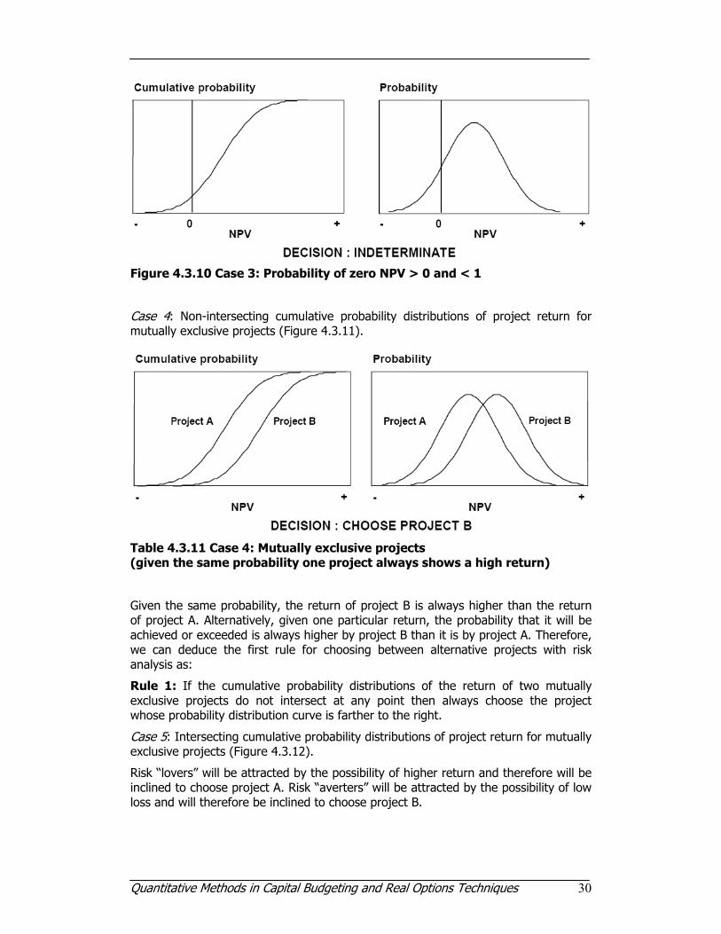
Figure 4.3.10 Case 3: Probability of zero NPV > 0 and < 1

Case 4: Non-intersecting cumulative probability distributions of project return for mutually exclusive projects (Figure 4.3.11).

Table 4.3.11 Case 4: Mutually exclusive projects (given the same probability one project always shows a high return)

Given the same probability, the return of project B is always higher than the return of project A. Alternatively, given one particular return, the probability that it will be achieved or exceeded is always higher by project B than it is by project A. Therefore, we can deduce the first rule for choosing between alternative projects with risk analysis as:

Rule 1: If the cumulative probability distributions of the return of two mutually exclusive projects do not intersect at any point then always choose the project whose probability distribution curve is farther to the right.

Case 5: Intersecting cumulative probability distributions of project return for mutually exclusive projects (Figure 4.3.12).

Risk “lovers” will be attracted by the possibility of higher return and therefore will be inclined to choose project A. Risk “averters” will be attracted by the possibility of low loss and will therefore be inclined to choose project B.


Rule 2: If the cumulative probability distributions of the return of two mutually exclusive projects intersect at any point then the decision rests on the risk predisposition of the investor.

Figure 4.3.12 Case 5: Mutually exclusive projects (high return vs. low loss)

With non-cumulative probability distributions a true intersection is harder to detect because probability is represented spatially by the total area under each curve.

Cost of Uncertainty

The cost of uncertainty, or the value of information as it is sometimes called, is a useful concept that helps determine the maximum amount of money one should be prepared to pay to obtain information in order to reduce project uncertainty. This may be defined as the expected value of the possible gains foregone following a decision to reject a project, or the expected value of the losses that may be incurred following a decision to accept a project.

The expected gain forgone from rejecting a project is illustrated in the right-hand diagram of Figure 4.3.13 by the sum of the possible positive NPVs weighted by their respective probabilities. Similarly, the expected loss from accepting a project, indicated in the left-hand diagram, is the sum of all the possible negative NPVs weighted by their respective probabilities.

By being able to estimate the expected benefit that is likely to result from the purchase of more information, one can decide on whether it is worthwhile to postpone a decision to accept or reject a project and seek further information or whether to make the decision immediately. As a general rule one should postpone the investment decision if the possible reduction in the cost of uncertainty is greater than the cost of securing more information (including foregone profits if the project is delayed).


Figure 4.3.13 Cost of Uncertainty

Expected Loss Ratio

The expected loss ratio (el) is a measure indicating the magnitude of expected loss relative to the project's overall expected NPV. This is expressed in the formula absolute value of expected loss divided by the sum of expected gain and absolute value of expected loss:

LossExpectedGainExpectedLossExpected

el

+

=

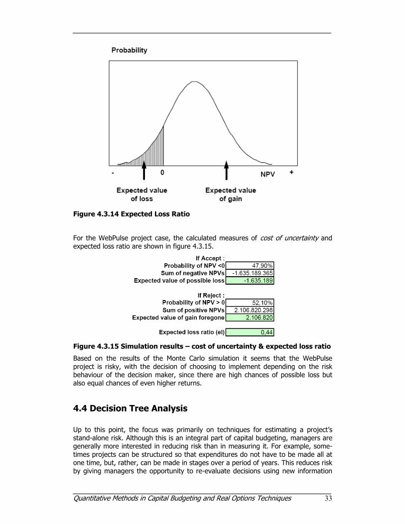
It can vary from 0, meaning no expected loss, to 1, which means no expected gain. Diagrammatically, this is the probability weighted return derived from the shaded area to the left of zero NPV divided by the probability weighted return derived from the total distribution whereby the negative returns are taken as positive (see Figure 4.3.14).

A project with a probability distribution of returns totally above the zero NPV mark would compute an el value of 0, meaning that the project is completely unexposed to risk. On the other hand, a project with a probability distribution of returns completely below the zero NPV mark would result in an el of 1, meaning that the project is totally exposed to risk.

The ratio does not therefore distinguish between levels of risk for totally positive or totally negative distributions. However, within these two extreme boundaries the el ratio could be a useful measure for summarising the level of risk to which a project may be subjected. The el ratio defines risk to be a factor of both the shape and the position of the probability distribution of returns in relation to the “cut-off” mark of zero NPV.


Figure 4.3.14 Expected Loss Ratio

For the WebPulse project case, the calculated measures of cost of uncertainty and expected loss ratio are shown in figure 4.3.15.

Figure 4.3.15 Simulation results – cost of uncertainty & expected loss ratio

Based on the results of the Monte Carlo simulation it seems that the WebPulse project is risky, with the decision of choosing to implement depending on the risk behaviour of the decision maker, since there are high chances of possible loss but also equal chances of even higher returns.

4.4 Decision Tree Analysis

Up to this point, the focus was primarily on techniques for estimating a project’s stand-alone risk. Although this is an integral part of capital budgeting, managers are generally more interested in reducing risk than in measuring it. For example, some-times projects can be structured so that expenditures do not have to be made all at one time, but, rather, can be made in stages over a period of years. This reduces risk by giving managers the opportunity to re-evaluate decisions using new information


and then either investing additional funds or terminating the project. Such projects can be evaluated using decision trees.

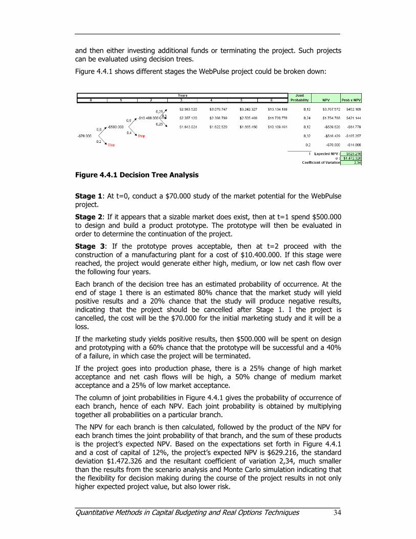
Figure 4.4.1 shows different stages the WebPulse project could be broken down:

Figure 4.4.1 Decision Tree Analysis

Stage 1: At t=0, conduct a $70.000 study of the market potential for the WebPulse project.

Stage 2: If it appears that a sizable market does exist, then at t=1 spend $500.000 to design and build a product prototype. The prototype will then be evaluated in order to determine the continuation of the project.

Stage 3: If the prototype proves acceptable, then at t=2 proceed with the construction of a manufacturing plant for a cost of $10.400.000. If this stage were reached, the project would generate either high, medium, or low net cash flow over the following four years.

Each branch of the decision tree has an estimated probability of occurrence. At the end of stage 1 there is an estimated 80% chance that the market study will yield positive results and a 20% chance that the study will produce negative results, indicating that the project should be cancelled after Stage 1. I the project is cancelled, the cost will be the $70.000 for the initial marketing study and it will be a loss.

If the marketing study yields positive results, then $500.000 will be spent on design and prototyping with a 60% chance that the prototype will be successful and a 40% of a failure, in which case the project will be terminated.

If the project goes into production phase, there is a 25% change of high market acceptance and net cash flows will be high, a 50% change of medium market acceptance and a 25% of low market acceptance.

The column of joint probabilities in Figure 4.4.1 gives the probability of occurrence of each branch, hence of each NPV. Each joint probability is obtained by multiplying together all probabilities on a particular branch.

The NPV for each branch is then calculated, followed by the product of the NPV for each branch times the joint probability of that branch, and the sum of these products is the project’s expected NPV. Based on the expectations set forth in Figure 4.4.1 and a cost of capital of 12%, the project’s expected NPV is $629.216, the standard deviation $1.472.326 and the resultant coefficient of variation 2,34, much smaller than the results from the scenario analysis and Monte Carlo simulation indicating that the flexibility for decision making during the course of the project results in not only higher expected project value, but also lower risk.


5. Real Options

The traditional discounted cash flow approach in capital budgeting assumes a single decision pathway with fixed outcomes, and all decisions are made in the beginning without the ability to change and develop over time. The real options approach considers multiple decision pathways as a consequence of high uncertainty coupled with management’s flexibility in choosing the optimal strategies or options along the way when new information becomes available. That is, management has the flexibility to make midcourse strategy corrections when there is uncertainty involved in the future. As information becomes available and uncertainty becomes resolved, management can choose the best strategies to implement. Traditional discounted cash flow assumes a single static decision, while real options assume a multidimensional dynamic series of decisions, where management has the flexibility to adapt given a change in the business environment.

What is an Option?

An option is the right, but not the obligation, to take an action in the future. Options are valuable when there is uncertainty. For example, one option contract traded on the financial exchanges gives the buyer the opportunity to buy a stock at a specified price on a specified date and will be exercised only if the price of the stock on that date exceeds the specified price. Many strategic investments create subsequent opportunities that may be taken, and so the investment opportunity can be viewed as a stream of cash flow plus a set of options.

In a narrow sense, the real options approach is the extension of financial option theory to options on real (nonfinancial) assets. While financial options are detailed in the contract, real options embedded in strategic investments must be identified and specified. Moving from financial options to real options requires a way of thinking, one that brings the discipline of the financial markets to internal strategic investment decisions.

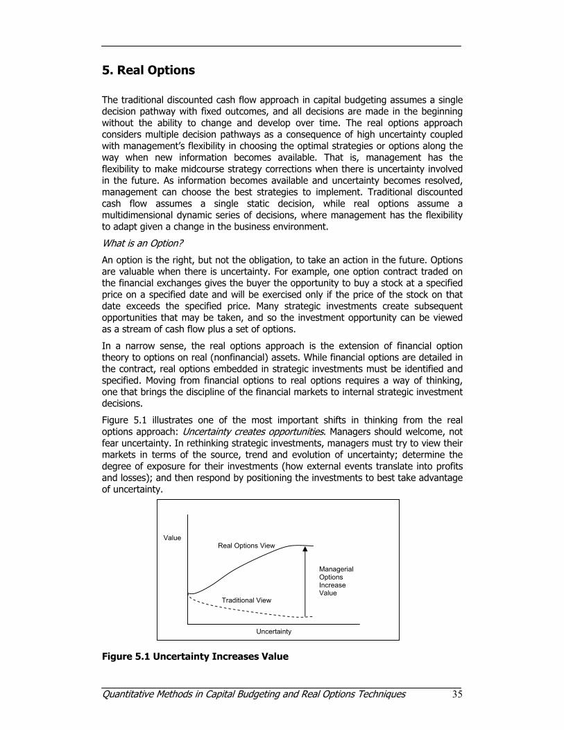
Figure 5.1 illustrates one of the most important shifts in thinking from the real options approach: Uncertainty creates opportunities. Managers should welcome, not fear uncertainty. In rethinking strategic investments, managers must try to view their markets in terms of the source, trend and evolution of uncertainty; determine the degree of exposure for their investments (how external events translate into profits and losses); and then respond by positioning the investments to best take advantage of uncertainty.

Figure 5.1 Uncertainty Increases Value

Uncertainty

Value

Managerial Options Increase Value

Traditional View

Real Options View


In the traditional view a higher level of uncertainty leads to a lower asset value. The real options approach shows that increased uncertainty can lead to a higher asset value if managers identify and use their options to flexibly respond to unfolding events.

The first step in valuing projects that have embedded options is to identify the options. Several types of real options are often present, and managers should always look out for them. Even more important, managers should try to create options within projects.

Investment Timing Options

Conventional NPV analysis implicitly assumes that projects will either be accepted or rejected, which implies that they will be undertaken now or never. In practice, however, companies sometimes have a third choice – delay the decision until later, when more information is available. Such investment timing options can dramatically affect a project’s estimated profitability and risk.

The option to delay is valuable only if it more than offsets any harm that might come from delaying. For example, if you delay, some other company might establish a loyal customer base that makes it difficult for your company to later enter the market. The option to delay is usually most valuable to firms with proprietary technology, patents, licenses, or other barriers to entry, because these factors lessen the threat of competition. The option to delay is valuable when market demand is uncertain, but it is also valuable during periods of volatile interest rates, since the ability to wait can allow firms to delay raising capital for projects until interest rates are lower.

Growth Options

A growth option allows a company to increase its capacity if market conditions are better than expected. There are several types of growth options. One lets a company increase the capacity of an existing product line. The second type of growth option allows a company to expand into new geographic markets. A third type of growth option is the opportunity to add new products, including complementary products and successive “generations” of the original product.

Abandonment Options

Many projects contain an abandonment option. When evaluating a potential project, standard DCF analysis assumes that the assets will be used over a specified economic life. While some projects must be operated over their full economic life, even though market conditions might deteriorate and cause lower than expected cash flows, others can be abandoned. Note also that some projects can be structured so that they provide the option to reduce capacity or temporarily suspend operations.

Flexibility Options

Many projects offer flexibility options that permit the firm to alter operations depending on how conditions change during the life of the project. Typically, either inputs or outputs (or both) can be changed.


5.1 Real Options Valuation Approach

The real options valuation approach can be summarised in the following steps:

Real Options Problem Framing

Real options are not specified in a contract, but must be identified through analysis and judgment. Developing a good application frame is the most important step in the real options approach. Based on the overall problem identification occurring during the initial qualitative management screening process, certain strategic optionalities would have become apparent for each particular project. The strategic optionalities may include, among other things, the option to expand, contract, abandon, switch, choose, and so forth. Based on the identification of strategic optionalities that exist for each project or at each stage of the project, the analyst can then choose from a list of options to analyze in more detail.

Real Options Modelling and Analysis

Through the use of Monte Carlo simulation, the resulting stochastic discounted cash flow model will have a distribution of values. In real options, we assume that the underlying variable is the future profitability of the project, which is the future cash flow series. An implied volatility of the future free cash flow or underlying variable can be calculated through the results of a Monte Carlo simulation previously performed. Usually, the volatility is measured as the standard deviation of the logarithmic returns on the free cash flows stream. In addition, the present value of future cash flows for the base case discounted cash flow model is used as the initial underlying asset value in real options modelling.

Portfolio and Resource Optimisation

Portfolio optimization is an optional step in the real options framework. If the analysis is done on multiple projects, management should view the results as a portfolio of rolled-up projects. This is because the projects are in most cases correlated with one another and viewing them individually will not present the true picture. As firms do not only have single projects, portfolio optimization is crucial. Given that certain projects are related to others, there are opportunities for hedging and diversifying risks through a portfolio. Because firms have limited budgets, have time and resource constraints, while at the same time have requirements for certain overall levels of returns, risk tolerances, and so forth, portfolio optimization takes into account all these to create an optimal portfolio mix. The analysis will provide the optimal allocation of investments across multiple projects.

Update Analysis

Real options analysis assumes that the future is uncertain and that management has the right to make midcourse corrections when these uncertainties become resolved or risks become known; the analysis is usually done ahead of time and thus, ahead of such uncertainty and risks. Therefore, when these risks become known, the analysis should be revisited to incorporate the decisions made or revising any input assumptions. Sometimes, for long-horizon projects, several iterations of the real options analysis should be performed, where future iterations are updated with the latest data and assumptions.


5.2 Timing Option - Decision Tree Method

Assuming the WebPulse project, the future cash flows depend on the demand for wireless internet browsing devices, which is uncertain. Let us assume that there is a 25% chance that demand for the new device will be very high, with first year sales of 48.000 units. There is a 50% chance of average demand, with first year sales of 38.000 units, and a 25% chance that demand will be low, with first year sales of 26.600 units.

The project could be implemented immediately, or it could be chosen to delay the decision until next year, when more information about demand would be available. In this case the investment will be made only if demand is sufficient to provide a positive NPV.

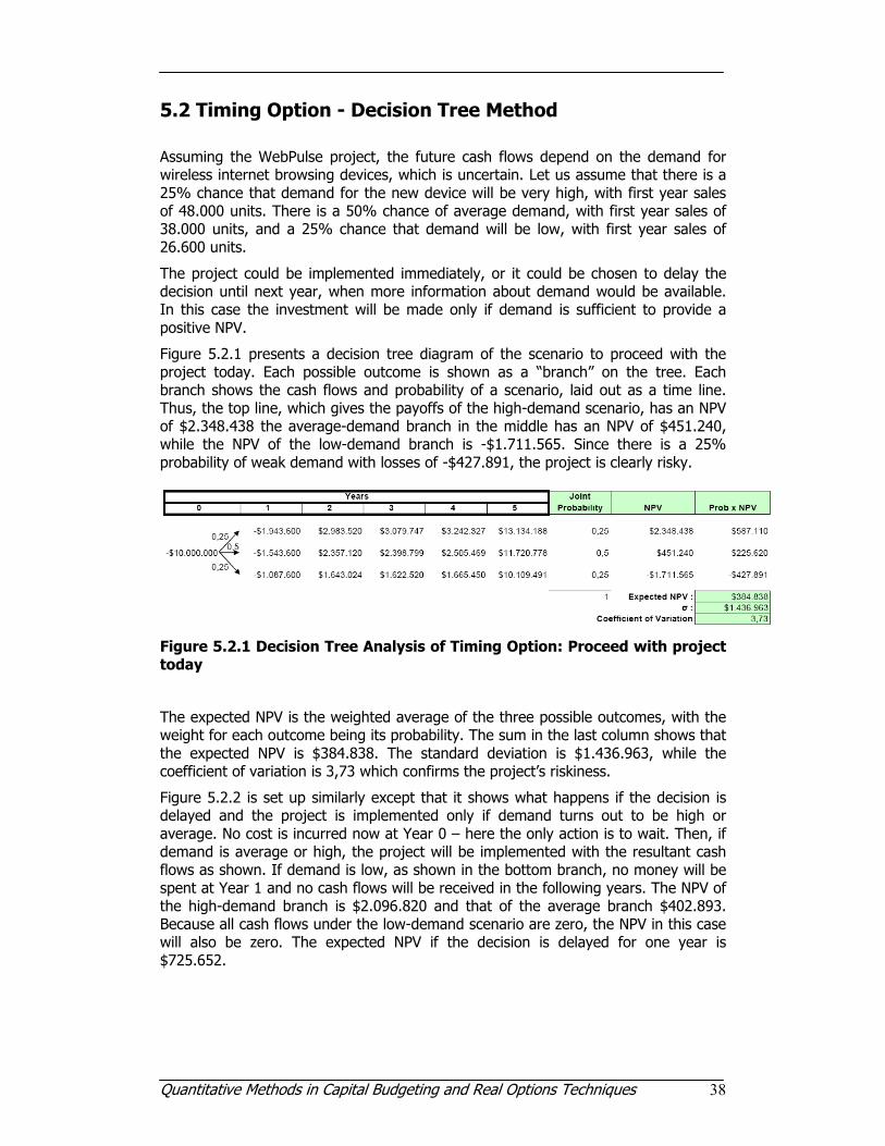
Figure 5.2.1 presents a decision tree diagram of the scenario to proceed with the project today. Each possible outcome is shown as a “branch” on the tree. Each branch shows the cash flows and probability of a scenario, laid out as a time line. Thus, the top line, which gives the payoffs of the high-demand scenario, has an NPV of $2.348.438 the average-demand branch in the middle has an NPV of $451.240, while the NPV of the low-demand branch is -$1.711.565. Since there is a 25% probability of weak demand with losses of -$427.891, the project is clearly risky.

Figure 5.2.1 Decision Tree Analysis of Timing Option: Proceed with project today

The expected NPV is the weighted average of the three possible outcomes, with the weight for each outcome being its probability. The sum in the last column shows that the expected NPV is $384.838. The standard deviation is $1.436.963, while the coefficient of variation is 3,73 which confirms the project’s riskiness.

Figure 5.2.2 is set up similarly except that it shows what happens if the decision is delayed and the project is implemented only if demand turns out to be high or average. No cost is incurred now at Year 0 – here the only action is to wait. Then, if demand is average or high, the project will be implemented with the resultant cash flows as shown. If demand is low, as shown in the bottom branch, no money will be spent at Year 1 and no cash flows will be received in the following years. The NPV of the high-demand branch is $2.096.820 and that of the average branch $402.893. Because all cash flows under the low-demand scenario are zero, the NPV in this case will also be zero. The expected NPV if the decision is delayed for one year is $725.652.


Figure 5.2.2 Decision Tree Analysis of Timing Option: Implement next year only if optimal

This analysis shows that the project’s expected NPV will be much higher if the project is implemented the next year instead of proceeding immediately. Additionally, the standard deviation is much lower and the coefficient of variation is only 1,11 indicating that this scenario is also much less riskier.

5.3 Timing Option - Black Scholes Model

It is often useful to obtain additional insights into the real option’s value by using an options pricing model. To do this, the analyst must find a standard financial option that resembles the project’s real option.

Note that the timing option mentioned for the WebPulse case resembles a call option on a stock. A call option gives its owner the right to purchase a stock at a fixed exercise price, but only if the stock’s price is higher than the exercise price will the owner exercise the option and buy the stock.

The value of a call option can be determined by using the Black-Scholes Option Pricing Model:

tdd

t

trXP

d

dNeXdNPV

RF

trRF

σ

σ

σ

−=

⋅++=

⋅⋅−⋅= −

12

2

1

21

])2

([)ln(

)()(

where:

V = Current value of call option

P = Current value of the underlying asset

X = Cost of Investment

rRF = Risk-free rate of return


t = time to expiration

σ = Volatility of the underlying asset

N(d1) and N(d2) are the value of the normal distribution at d1 and d2

This equation requires five inputs: (1) the risk-free rate, (2) the time until the option expires, (3) the exercise price, (4) the current price of the stock, (5) the variance of the stock’s rate of return. Therefore, values need to be estimated for those five inputs.

(1) The risk free rate is assumed to be 5%.

(2) The decision upon whether or not to implement the project should be made in a year, so there is one year until the option expires.

(3) It will cost $10.000.000 to implement the project, so the same amount is used for the exercise price X.

(4) We need a proxy for the value of the underlying asset, which in Black-Scholes is the current price of the stock. Note that a stock’s current price is the present value of its expected future cash flows. For the WebPulse case, the underlying asset is the project itself, and its current “price” is the present value of its expected future cash flow. Therefore, as a proxy for the stock price we can use the present value of the project’s future cash flows.

(5) The variance of the project’s expected return can be used to represent the variance of the stock’s return in the Black-Scholes model.

Figure 5.2.1 shows how one can estimate the present value of the project’s cash inflows. The current value of the underlying asset is needed to be found, that is the value of the project. For a stock, the current price is the present value of all expected future cash flow, including those that are expected even if we do not exercise the call option. Note also that the exercise price for a call option has no effect on the stock’s current price. For our real option, the underlying asset is the delayed project, and its current “price” is the present value of all its future expected cash flows. Just as the price of a stock includes all of its future cash flows, the present value of the project should include all its possible future cash flows. Moreover, since the price of a stock is not affected by the exercise price of a call option, we ignore the project’s “exercise price”, or cost, when we find its present value. Figure 5.2.1 shows the expected cash flows if the project is delayed. The present value of these cash flows as of now (Year 0) is $9.272.177, and this is the input we should use for the current price in the Black-Scholes model.

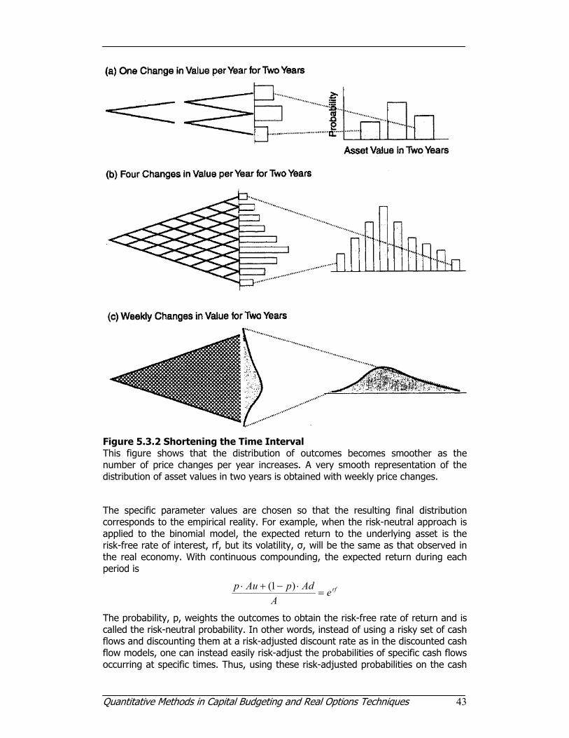
Figure 5.2.1 Estimation of value of underlying asset


The last required input is the variance of the project’s return. As calculated in Appendix A2, as the volatility of the logarithmic returns of the future cash flows, it is found to be 59,57%. This method is usually calculated on a large amount of available data values. This is not the case for the WebPulse project thus the result cannot be fully trusted.

Another approach for estimating the variance takes into account the fact that demand is not really limited to the three scenarios – rather, a wide range of outcomes is possible. Similarly, the stock price at the time a call option expires could take on one of many values. It is reasonable to assume that the value of the project at the time when we must decide on undertaking it behaves similarly to the price of a stock at the time a call option expires. Under this assumption, we can use the expected value and standard deviation of the project’s value to calculate the variance of its rate of return, σ2, with the following formula:

tCV )1ln( 2

2 +=σ

Here CV is the coefficient of variation of the underlying asset’s price at the time the option expires and t is the time until the option expires. Thus, while the three scenarios are simplifications of the true condition, where there are an infinite number of possible outcomes, we can still use the scenario data to estimate the variance of the project’s rate of return if it has an infinite number of possible outcomes.

For the WebPulse project, this method produces the following estimate of the variance of the project’s return:

%20189,01

)114,0ln( 22 ==

+=σ

Applying the above estimated values to the Black-Scholes formula yields a result of $404.394 as shown in Figure 5.2.2. Since this value is higher than the $384.838 NPV under immediate implementation, we conclude that the final decision to proceed or not with the project should be made in one year when more information will be available.

Figure 5.2.2 Application of Black-Scholes Model


5.3 Binomial Lattice – Growth & Abandonment Option

Closed-form solutions are models like the Black-Scholes, where there exist equations that can be solved given a set of input assumptions. They are exact, quick, and easy to implement with the assistance of some basic programming knowledge but are difficult to explain because they tend to apply highly technical stochastic calculus mathematics. They are also very specific in nature, with limited modelling flexibility. Binomial lattices, in contrast, are easy to implement and easy to explain.

The binomial option valuation model is based on a simple representation of the evolution of the value of the underlying asset. In each time period the underlying asset can take only one of two possible values. As Figure 5.3.1 shows, the up or down movements lay out the possible paths.

In the most widely used version, the multiplicative binomial model of uncertainty, the asset has an initial value, A, and within a short time period either moves up to Au or down to Ad. Figure 5.3.1(a) shows the binomial tree and how it results in a distribution of outcomes on the final date. Each bar on the distribution is placed at a single outcome, and as Figure 5.3.1(b) shows, the height of the bar is the frequency of obtaining that outcome over all possible paths in the binomial tree.

Figure 5.3.1 The Binomial Representation of Uncertainty (a) In each short time interval the value of the asset A increases by u or decreases by d. Future asset values are calculated in the binomial tree. (b) At the final date, the distribution of possible asset values can be flipped over to its more familiar horizontal form.

The binomial representation of uncertainty is very flexible. Figure 5.3.2 shows that as the interval of time between changes in value grows shorter, the final distribution of outcomes becomes smoother. When the underlying asset changes value once per year, as shown in Figure 5.3.2(a), only three outcomes are possible at the end of two years, as in Figure 5.3.2(b). A very smooth representation of the final distribution is possible with weekly periods, as in Figure 5.3.2(c).


Figure 5.3.2 Shortening the Time Interval This figure shows that the distribution of outcomes becomes smoother as the number of price changes per year increases. A very smooth representation of the distribution of asset values in two years is obtained with weekly price changes.

The specific parameter values are chosen so that the resulting final distribution corresponds to the empirical reality. For example, when the risk-neutral approach is applied to the binomial model, the expected return to the underlying asset is the risk-free rate of interest, rf, but its volatility, σ, will be the same as that observed in the real economy. With continuous compounding, the expected return during each period is

rfeA

AdpAup=

⋅−+⋅ )1(

The probability, p, weights the outcomes to obtain the risk-free rate of return and is called the risk-neutral probability. In other words, instead of using a risky set of cash flows and discounting them at a risk-adjusted discount rate as in the discounted cash flow models, one can instead easily risk-adjust the probabilities of specific cash flows occurring at specific times. Thus, using these risk-adjusted probabilities on the cash


flows allows the analyst to discount these cash flows (whose risks have now been accounted for) at the risk-free rate. This is the essence of binomial lattices as applied in valuing options. The results obtained are identical.

Similarly, equating the variance of the return from the binomial model to that of the observed normal distribution gives:

2222 ])1([)1( σ=−+−−+ dppudppu

One solution to the above equations that assumes the underlying asset has symmetric up and down movements (i.e., u = 1/d) is given by:

)()(

1

)()(

dudep

eu

d

eu

tbrf

t

t

−−

=

==

=

⋅−

−

δ

δσ

δσ

The basic inputs are the present value of the underlying asset (S), present value of implementation cost of the option (X), volatility of the natural logarithm of the underlying free cash flow returns in percent (σ), time to expiration in years (T), risk-free rate or the rate of return on a riskless asset (rf), and continuous dividend outflows in percent (b). In addition, the binomial lattice approach requires two additional sets of calculations, the up and down factors (u and d) as well as a risk-neutral probability measure (p). We see from the equations above that the up factor is simply the exponential function of the cash flow volatility multiplied by the square root of time-steps or stepping time (δt). Time-steps or stepping time is simply the time scale between steps. That is, if an option has a one-year maturity and the binomial lattice that is constructed has 10 steps, each time-step has a stepping time of 0.1 years. The volatility measure is an annualized value; multiplying it by the square root of time-steps breaks it down into the time-step’s equivalent volatility. The down factor is simply the reciprocal of the up factor. In addition, the higher the volatility measure, the higher the up and down factors. This reciprocal magnitude ensures that the lattices are recombining because the up and down steps have the same magnitude but different signs; at places along the future path these binomial bifurcations must meet.

The second required calculation is that of the risk-neutral probability, defined simply as the ratio of the exponential function of the difference between risk-free rate and dividend, multiplied by the stepping time less the down factor, to the difference between the up and down factors. This risk-neutral probability value is a mathematical intermediate and by itself has no particular meaning. One major error real options users commit is to extrapolate these probabilities as some kind of subjective or objective probabilities that a certain event will occur – which is erroneous. There is no economic or financial meaning attached to these risk-neutralized probabilities apart from the fact that it is an intermediate step in a series of calculations. Having determined these values, the binomial lattice of the underlying asset value can be calculated, as shown in Figure 5.3.3.

Starting with the present value of the underlying asset at time zero (S0), multiply it with the up (u) and down (d) factors as shown below, to create a binomial lattice. Note that there is one bifurcation at each node, creating an up and a down branch.


The intermediate branches are all recombining. This evolution of the underlying asset shows that if the volatility is zero, in a deterministic world where there are no uncertainties, the lattice would be a straight line, and a discounted cash flow model will be adequate because the value of the option or flexibility is also zero. In other

words, if volatility (σ) is zero, then the up ( teu δσ= ) and down ( ted δσ−= ) jump sizes are equal to one. It is because there are uncertainties and risks, as captured by the volatility measure, that the lattice is not a straight horizontal line but comprises up and down movements. It is this up and down uncertainty that generates the value in an option. The higher the volatility measure, the higher the up and down factors as previously defined, the higher the potential value of an option as higher uncertainties exist and the potential upside for the option increases.

Figure 5.3.3 Binomial Lattice of the Underlying Asset Value

In any options model, there is a minimum requirement of at least two lattices. The first lattice is always the lattice of the underlying asset, while the second lattice is the option valuation lattice.

Back to WebPulse project case, let us assume that choosing to implement the WebPulse project gives management the option to expand and double its operation by further investing another $500.000 at any time over the next five years. What is the total value of the project taking into account this growth option? Three steps need to be followed for the Binomial Lattice approach, Rolling Forward the value of the underlying asset, Establishing the Decision Rule and Folding Back the future values to the present.

Rolling Forward

Figure 5.3.4 shows the rollout of the binomial tree for the value of the WebPulse project. Upward movements in the tree are along the row and downward movements are along the diagonal. The present value of the underlying asset is $451.240 as calculated from the base case NPV analysis, the volatility σ of the natural logarithm of the projects cash flows is 77,18% as calculated in Appendix A.2. The risk-free rate is assumed 5%. The time to expiration is 5 years and the lattice is calculated in 5 steps, so the stepping-time turns out to be 1. Applying the binomial lattice equations, the u is calculated as 2,16, while d as 0,46. Hence, starting with the underlying value of $451.240, we multiply this value with the up and down factors to obtain $976.329 and $208.554, respectively.


Figure 5.3.4 Valuation of Growth Option with Binomial Lattice Model

The tree shows that in 5 years the value of WebPulse might range from $9.516 to $21.396.888. Each endpoint is not very likely, but it is quite different from the current value of $451.240.

Establishing the Decision Rule

The next step is to establish the decision rule. At the end of 5 years there is an option to either expand, by spending $500.000 and doubling the operations or do nothing. Thus the value of the project is the maximum between expansion or continuation since management will choose the strategy that maximises profitability. At node G23 the value of acquiring and expanding its operations is equivalent to doubling its existing capacity of $21.396.888 at the same node of the rolling forward lattice G13. Hence, the value of acquiring and expanding the firm’s operations is double this existing capacity less any acquisition costs, or 2 x $21.396.888 - $500.000 = $42.293.776.

Folding Back the Values

The final step in the binomial option valuation is to bring back future values to the present. Since management has the option of growth not only on year 5, but can exercise this option at the end of any year until year 5, the decision rule of maximizing value is applied in parallel to folding back the values. For example, the node F27 is calculated as the maximum between the decision rule establish earlier or the folded back value of nodes G27 and G28. For this node the folded back value at year 4 is:


[44.549 p + 9.516 (1-p)]e-rf = 20.589

which is greater than 2 x $20.589 - $500.000 = -$458.822

The remainder of the tree is filled in the same manner, resulting in a current value of WebPulse of $746.914 considerably higher than the initial $451.240 without the growth option. The growth option itself can be valued as the difference between WebPulses value with and without the option, thus:

Growth Option Value = $746.914 - $451.240 = $295.673

The real options value is worth an additional 65 percent of existing business operations. If a real options approach is not used, the project will be undervalued because there is a strategic option to expand its current operations but not an obligation to do so and will most likely not do so unless market conditions deem it optimal. Having an option and sometimes keeping this option open are valuable given a highly uncertain business environment.

Let us now assume that instead of the growth option, there exists the option of abandonment, where management may choose to abandon the project at any time until the end of year 5 and collect the salvage values of the invested assets including the building and equipment.

Figure 5.3.5 shows the relevant calculations, where the salvage values of the assets for each year (row 11) are taken from the results of Figure 2.2.2.

Figure 5.3.5 Valuation of Growth Option with Binomial Lattice Model

As can be seen from Figure 5.3.5 the value of the project with the abandonment option results to $8.678.636, while the option itself is worth $8.227.396.


5.4 Geometric Brownian Motion Simulation Model

Figure 5.4.1 shows a “cone of uncertainty,” where we can depict uncertainty as increasing over time. Notice that risk may or may not increase over time, but uncertainty does increase over time. For instance, it is usually much easier to predict business conditions a few months in advance, but it becomes more and more difficult the further one goes into the future, even when business risks remain unchanged. This is the nature of the cone of uncertainty. If we were to attempt to forecast future cash flows while attempting to quantify uncertainty using simulation, a well prescribed method is to simulate thousands of cash flow paths over time, as shown in Figure 5.4.1. Based on all the simulated paths, a probability distribution can be constructed at each time period.

Figure 5.4.1 The Cone of Uncertainty

Based on the cone of uncertainty, which depicts uncertainty as increasing over time, we can clearly see the similarities in triangular shape between a cone of uncertainty and a binomial lattice as shown in Figure 5.3.3. In essence, a binomial lattice is simply a discrete simulation of the cone of uncertainty. Brownian Motion on the other hand is a continuous stochastic simulation process. The simulated pathways of Figure 5.4.1 were generated using a Geometric Brownian Motion with a fixed volatility. A Geometric Brownian Motion can be depicted as:

ttSS δσεδµδ

+= )(

Where a percent change in the variable S (denoted SSδ

) is a combination of a

deterministic part (µ(δt)) and a stochastic part ( tδσε ). Here, µ is a drift term or growth parameter that increases at a factor of time-steps δt, while σ is the volatility parameter, growing at a rate of the square root of time, and ε is a simulated variable, usually following a normal distribution with a mean of zero and a variance


of one. Note that the different types of Brownian Motions are widely regarded and accepted as standard assumptions necessary for pricing options. Brownian Motions are also widely used in predicting stock prices.

Notice that the volatility (σ) remains constant throughout several thousand simulations. Only the simulated variable (ε) changes every time. Although the risk or volatility measure (σ) in this example remains constant over time, the level of uncertainty increases over time at a factor of ( tδσ ). That is, the level of uncertainty grows at the square root of time and the more time passes, the harder it is to predict the future. This is seen in the cone of uncertainty, where the width of the cone increases over time.

In the Geometric Brownian Motion simulation model, instead of predicting the future values of the underlying asset with a binomial lattice, the Brownian motion equation is used. Figure 5.4.2 shows a sample of the simulation for the WebPulse project. In this case the value of the growth option will be calculated, where management has the option of doubling the operations of the project by investing another $500.000. The difference between the stochastic process simulation and the binomial lattice approach in paragraph 5.3 is that the stochastic simulation does not permit the performance of decision rules when folding back. This is equivalent to a European type call option, where the option to expand can only be exercised at the end of the expiration period and not until the end of the expiration period as in an American type call option.

Figure 5.4.2 Growth Option Calculation with Geometric Brownian Motion Simulation


The first step is to determine the number of steps to simulate. In the WebPulse case 100 steps were chosen (Figure 5.4.2 depicts only the first 15). Starting with the initial asset value of $451.240 (S0), the change in value from this initial value to the first period is seen as ))((01 ttrfSS δσεδδ +⋅= . Hence, the value of the asset at the first time-step is equivalent to:

))((00101 ttrfSSSSS δσεδδ +⋅+=+=

The value of the asset at the second time-step is hence:

))((11212 ttrfSSSSS δσεδδ +⋅+=+=

and so forth, all the way until the terminal 100th time-step.

Notice that because ε changes on each simulation trial, each simulation trial will produce an entirely different asset evolution pathway. At the end of the 100th time-step, the maximization process is then applied. That is, for the growth option with a $500.000 implementation cost, the function is Max[2 x S10,i - X, 0]. This is the call value C100,i at time 100 for the ith simulation trial. This value is then discounted at the risk-free rate to obtain the call value at time zero, that is:

)(,100,0

Trfii eCC −⋅=

This is a single-value estimate for a single simulated pathway.

Applying simulation runs for 1000 trials (only 49 are depicted in Figure 5.4.2) and obtaining the mean value of C0 yeilds $519.790. Obviously, the higher the number of simulations and the higher the number of steps in the simulation, the more accurate the results. The result, as in the binomial lattice valuation case, suggests there is high value in the project taking into account the option of growth.


6. Conclusions

Having examined a wide range of capital budgeting valuation techniques the following observations can be made.

Traditional valuation methods have several drawbacks with regards to their assumptions and are summarized in the following table:

Assumptions Realities

Decisions are made now, and cash flow streams are fixed for the future.

Uncertainty and variability in future outcomes. Not all decisions are made today, as some may be deferred to the future, when uncertainty becomes resolved.

Projects are “mini firms,” and they are interchangeable with whole firms.

With the inclusion of network effects, diversification, interdependencies, and synergy, firms are portfolios of projects and their resulting cash flows. Sometimes projects cannot be evaluated as stand-alone cash flows.

Once launched, all projects are passively managed.

Projects are usually actively managed through project life cycle, including checkpoints, decision options, budget constraints, and so forth.

Future free cash flow streams are all highly predictable and deterministic.

It may be difficult to estimate future cash flows as they are usually stochastic and risky in nature.

Project discount rate used is the opportunity cost of capital, which is proportional to non-diversifiable risk.

There are multiple sources of business risks with different characteristics, and some are diversifiable across projects or time.

All risks are completely accounted for by the discount rate.

Firm and project risk can change during the course of a project.

All factors that could affect the outcome of the project and value to the investors are reflected in the DCF model through the NPV or IRR.

Because of project complexity and so-called externalities, it may be difficult or impossible to quantify all factors in terms of incremental cash flows. Distributed, unplanned outcomes (e.g., strategic vision and entrepreneurial activity) can be significant and strategically important.

Unknown, intangible, or immeasurable factors are valued at zero.

Many of the important benefits are intangible assets or qualitative strategic positions.

Monte Carlo analysis is a useful tool extending the depth of project appraisal and enhancing the investment decision. The following specific advantages for risk analysis can be highlighted:

1. It enhances decision making on marginal projects. A project whose single-value NPV is small may still be accepted following risk analysis on the grounds that its overall chances for yielding a satisfactory return are greater than is the probability of


making an unacceptable loss. Likewise, a marginally positive project could be rejected on the basis of being excessively risky, or one with a lower NPV may be preferred to another with a higher NPV because of a better risk/return profile.

2. It screens new project ideas and aids the identification of investment opportunities. Very often a new project concept is formulated that needs to be developed into a business opportunity. Before any real expenses are incurred to gather information for a full feasibility study it is possible to apply risk analysis widening the margins of uncertainty for the key project variables to reflect the lack of data. A substantial investment of human and financial resources is not incurred until the potential investors are satisfied that the preliminary risk/return profile of the project seems to be acceptable.

3. It highlights project areas that need further investigation and guides the collection of information. Risk analysis can contain the costs of investigation and fieldwork aiming at improving the accuracy of a forecast relating to particular project variables. If the cost for obtaining such information is greater than the expected benefit likely to result from the purchase of the information then the expense is not justified.

4. It aids the reformulation of projects to suit the attitudes and requirements of the investor. A project may be redesigned to take account for the particular risk predispositions of the investor.

5. It induces the careful re-examination of the single-value estimates in the deterministic appraisal. The difficulty in specifying range limits and probability distributions for risk analysis often resides in the fact that the projected values are not adequately researched. The need to define and support explicit assumptions in the application of risk analysis therefore forces the analyst to also critically review and revise the base-case scenario.

6. It helps reduce project evaluation bias through eliminating the need to resort to conservative estimates as a means of reflecting the analyst's risk expectations and predispositions.

7. It facilitates the thorough use of experts who usually prefer to express their expertise in terms of a probability distribution rather than having to compress and confine their opinion in a single value.

8. It bridges the communication gap between the analyst and the decision maker. The execution of risk analysis in a project appraisal involves the collection of information which to a large part reflects the acquired knowledge and expertise of top executives in an organisation. By getting the people who have the responsibility of accepting or rejecting a project to agree on the ranges and probability distributions used in risk analysis the analyst finds an invaluable communication channel through which the major issues are identified and resolved. The decision maker in turn welcomes his involvement in the risk analysis process as he recognises it to be an important management decision role which also improves his/her overall understanding of the appraisal method.

9. It supplies a framework for evaluating project result estimates. Unlike the prediction of deterministic appraisal which is almost always refuted by the actual project result, the probabilistic approach is a methodology which facilitates empirical testing.

10. It provides the necessary information base to facilitate a more efficient allocation and management of risk among various parties involved in a project. Once the various sources of risk have been assessed, project risk may be contractually


allocated to those parties who are best able to bear it and/or manage it. Moreover, it enables the testing of possible contractual arrangements for the sale of the products or the purchase of project inputs between various parties until a satisfactory formulation of the project is achieved.

Comparing the approach used in a traditional Discounted Cash Flow (DCF) method to Real Options, since we can define risk as uncertain fluctuations in revenues and the NPV level, all downside risks are mitigated in Real Options because you do not execute a project if the nominal or worst-case scenario occurs in time. In retrospect, the upside risks are maximized such that the returns are increased because a project will only be executed when the best-case scenario occurs. This creates a win-win situation where risks are mitigated and returns are enhanced, simply by having the right strategic optionalities available, acting appropriately, and valuing the project in terms of its “real” or intrinsic value, which includes this opportunity to make midcourse corrections when new information becomes available. So from a “wide” distribution with low returns as a result of DCF analysis, the Real Options approach displays a “tigher” distribution with higher returns as shown below.

Closed-form solutions like the Black-Scholes model, where equations exist that can be solved given a set of input assumptions are exact, quick, and easy to implement with the assistance of some basic programming knowledge but are difficult to explain because they tend to apply highly technical stochastic calculus mathematics. They are also very specific in nature, with limited modelling flexibility. Binomial lattices, in contrast, are easy to implement and easy to explain. They are also highly flexible but require significant computing power and time-steps to obtain good approximations.


References

Amram M. & Kulatilaka N., ”Real Options – Managing Strategic Investment in an Uncertain World”, Harvard Business School Press, Boston, Massachusetts, 1999. Schilling M.A., “Strategic Management of Technological Innovation”, McGraw Hill International Anthony, Hawkins, Merchant, “Accounting – Text & Cases”, McGraw Hill International Dayananda D., Irons R., Harrison S., Jerbohn J. & Rowland P., “Capital Budgeting : Financial Appraisal of Investment Projects”, Cambridge University Press, 2002 Savvakis C. Savvides, “Risk Analysis in Investment Appraisal”, Beech Tree Publishing, 1994. Brigham E. F., Ehrhardt M. C., “Financial Management: Theory and Practice”, Thomson – South West Mun J., “Real Options Analysis: Tools and Techniques for Valuing Strategic Investments and Decisions”, John Wiley & Sons Luenberger D. G., “Investment Science”, Oxford University Press, 1998 Iatropoulos A., Economidis A. & Angelou G., “Broadband Investments Analysis Using Real Options Methodology. A case study for Egnatia Odos S.A.”, “Communications & Strategies”, no. 55, 2004 Benaroch M. & Kauffmann R., “A case for using real options pricing analysis to evaluate information technology project investments”, “Information Systems Research”, vol. 10, No. 1, p.p. 70-86, 1999 Smit H.T.J. & Trigeorgis L., “Quantifying the Strategic Option Value of Technology Investments”. Galimaridou A., Houlis P., Pitsikalis C., Theodoropoulos D., “WebPulse & MyWeb Business Plan”, Athens Information Technology, 2007


Appendix

A.1 Time Value of Money

A dollar in hand today is worth more than a dollar to be received in the future because, if you had it now, you could invest it, earn interest and end up with more than one dollar in the future. The process of going from today’s values, or present values (PVs), to future values (FVs) is called compounding.

In general, the future value of an initial lump sum at the end of n years can be found by applying the formulae:

nn iPVFV )1( +⋅=

Where i equals the interest rate per year.

The process of finding present values from future values is called discounting and is the reverse of compounding. Thus,

nn i

FVPV )1

1(+

⋅=


A.2 Estimation of Volatility – Logarithmic Cash Flow Returns Approach

The logarithmic cash flow returns approach calculates the volatility using the individual future cash flow estimates and their corresponding logarithmic returns, as illustrated below in Table A.2.1. Starting with a series of forecast future cash flows, convert them into relative returns. Then take the natural logarithms of these relative returns. The standard deviation of these natural logarithm returns is the volatility of the cash flow series used in a real options analysis. Notice that the number of returns is one less than the total number of periods. That is, for time periods 0 to 5, we have six cash flows but only five cash flow returns.

Table A.2.1 Future Cash Flow Estimates and their Corresponding Logarithmic Returns

The volatility estimate is then calculated as:

%58.25)(1

11

2 =−−

= ∑=

n

ii xx

nvolatility

where n is the number of Xs, and x is the average X value. Clearly there are advantages and shortcomings to this simple approach. This method is very easy to implement, and Monte Carlo simulation is not required in order to obtain a single-point volatility estimate. This approach is mathematically valid and is widely used in estimating volatility of financial assets. However, for real options analysis, there are several caveats that deserve closer attention, including when cash flows are negative over certain time periods. That is, the relative returns will be a negative value, and the natural logarithm of a negative value does not exist. Hence, the volatility measure does not fully capture the possible cash flow downside and may produce erroneous results. In addition, auto-correlated cash flows (estimated using time-series forecasting techniques) or cash flows following a static growth rate will yield volatility estimates that are erroneous. Care should be taken in such instances.

Monte Carlo simulation can also be used in creating the discounted cash flow model that is used to calculate the cash flows, thereby running thousands of trials and reducing the risk of obtaining a single erroneous volatility estimate. Performing a Monte Carlo simulation at the discounted cash flow level is highly appropriate because a distribution of volatilities can be obtained and used as input into a real options analysis. The results of such an analysis will then yield a forecast distribution


of real options values, with its relevant probabilities of occurrence, rather than a single-point estimate.

Applying the above mentioned methodology to the WebPulse case yields the results presented in Figure A.2.2.

Figure A.2.2. Volatility Estimation for WebPulse Project

Date post:	27-Oct-2014
Category:	Documents
Upload:	pimpim-honeybee
View:	168 times
Download:	0 times

Capital Budgeting Techniques and Real Option

Documents