DI

SC

US

SI

ON

P

AP

ER

S

ER

IE

S

Forschungsinstitut zur Zukunft der ArbeitInstitute for the Study of Labor

Capital Income Taxation and the Mirrlees Review

IZA DP No. 6615

June 2012

Patricia AppsRay Rees

Capital Income Taxation and the

Mirrlees Review

Patricia Apps Sydney University Law School

and IZA

Ray Rees CES, University of Munich

Discussion Paper No. 6615 June 2012

IZA

P.O. Box 7240 53072 Bonn

Germany

Phone: +49-228-3894-0 Fax: +49-228-3894-180

E-mail: iza@iza.org

Any opinions expressed here are those of the author(s) and not those of IZA. Research published in this series may include views on policy, but the institute itself takes no institutional policy positions. The Institute for the Study of Labor (IZA) in Bonn is a local and virtual international research center and a place of communication between science, politics and business. IZA is an independent nonprofit organization supported by Deutsche Post Foundation. The center is associated with the University of Bonn and offers a stimulating research environment through its international network, workshops and conferences, data service, project support, research visits and doctoral program. IZA engages in (i) original and internationally competitive research in all fields of labor economics, (ii) development of policy concepts, and (iii) dissemination of research results and concepts to the interested public. IZA Discussion Papers often represent preliminary work and are circulated to encourage discussion. Citation of such a paper should account for its provisional character. A revised version may be available directly from the author.

IZA Discussion Paper No. 6615 June 2012

ABSTRACT

Capital Income Taxation and the Mirrlees Review*

The Mirrlees Review of the UK tax system, together with its companion volume of research papers, can be expected to influence future discussions of tax reform. Indeed, this can already be recognised in the Henry Review. As far as income taxation is concerned, the most substantive recommendation of the Mirrlees Review is a move toward a system of consumption or expenditure taxation, by exempting the “normal return” to saving and taxing only “excess returns” on the same tax schedule as labour earnings. This paper argues against this direction of reform on the grounds that it is based on a model of household behaviour over the life cycle that ignores important aspects of reality. We present an alternative model, together with supporting empirical evidence. We go on to argue that, against the background of rising inequality and an aging population, the appropriate direction for reform is towards more progressive taxation of both labour earnings and capital income, although not necessarily under the same rate scale. JEL Classification: H21, H24, H31, D13, D91, J22 Keywords: optimal taxation, labour supply, capital income taxation, family life cycle,

time allocation, saving, inequality Corresponding author: Patricia Apps Faculty of Law University of Sydney Eastern Avenue, Camperdown Campus Sydney NSW 2006 Australia E-mail: patricia.apps@sydney.edu.au

* We are grateful to James Banks, Michael Devereux, Rachel Griffith and Alan Marin, as well as other participants at the Oxford/Sydney conference on Taxation and the Manchester Economics Seminar, for helpful comments on this paper. The work was supported under the Australian Research Council’s Discovery Project funding scheme (DP1094021).

1 Introduction

The Mirrlees Review of the UK tax system1 together with its companion volumeof research papers2 make an important contribution to the literature on thetheory and policy of taxation, which can be expected to have an impact onfuture discussions of reform in a number of countries. Aspects of the review’sapproach foreshadowed in the research papers can for example be recognised asan influence on the recent Henry Review of the Australian tax system.3 Thispaper makes no attempt to survey the whole of the Mirrlees Review, but insteadaims to contribute to the discussion of the review by focusing on the issue ofthe taxation of the return to capital received directly as household income.4

However, in doing so it is also necessary to discuss its basic approach towardsthe taxation of income in general, both from labour earnings and saving. Thuswe are concerned with the arguments presented in Chapters 2-5, 13 and 14 ofTax by Design.In the next section of this paper we discuss critically the arguments for a

move away from the taxation of earnings from both labour and capital to asystem of consumption or expenditure taxation that are set out in these chap-ters. The basis for this criticism is that the implicit model of the householdunderlying the review’s proposals is inadequate to deal with the central issuesof tax design. In Section 3 we give a brief overview of the empirical work whichsupports this contention. In the section following we go on to examine theparticular proposal to exempt the "normal return to capital" from taxation,subjecting "excess returns" to the same tax schedule as labour earnings. Thisappears to be the main substantive innovation the review proposes in this area.Section 5 concludes.

2 Principles and proposals

In Chapters 2 and 3 the review makes clear its adherence to the professedstarting point of the modern theory of optimal taxation: Ideally we would like totax the innate productivity or earning capacity of individual income earners, butsince this is unobservable we are forced instead to generate distortions by taxing,inter alia, incomes and consumption, thus creating deadweight welfare losses asthe cost of funding the supply of public outputs and income redistribution.Then the goal of a tax system is to achieve an in some sense optimal balancebetween the effi ciency costs and equity benefits of taxation, for any given level ofreal public output. Less clear however is the way in which the review’s specificproposals in the area with which we are concerned could be expected to helpachieve this goal.

1Mirrlees et. al. (2011).2Mirrlees et. al. (2010).3See Australia’s Future Tax System Review Panel (2009).4That is, we also leave to one side the issues surrounding corporate taxation.

2

2.1 Changing the tax base from income to consumption

The review is clearly strongly in favour of changing the tax base from income -labour earnings plus returns to saving - to consumption. It presents three mainways in which this can be achieved:1. A cash flow expenditure tax, or EET: Withdrawals from income for

saving are tax exempt (E), income from saving is tax exempt (E), and then theproceeds are taxed when spent on consumption (T). This is in fact how pensionsaving is treated in the UK, where private pension wealth accounts on averagefor about 75% of financial (i.e. non-housing) wealth.2. A labour earnings tax with exemption for income from saving, or TEE:

Saving is made out of taxed income with no exemption (T), but returns (E)and final consumption of proceeds (E) are tax-exempt. This is essentially howhousing wealth is treated in the UK.3. An income tax with an "allowed rate of return", or TtE: Saving is made

out of taxed income (T), returns to saving at a rate below a certain level, the"normal rate of return", are tax exempt, while returns above this are taxed atthe same rate as labour earnings (t), and withdrawal of savings for consumptionare tax-exempt (E). The "normal rate of return" could, it is suggested, bebased on the real rate of return of 10-year UK government bonds (in numericalillustrations the review uses 5%), which of course, if only because of the risk ofinflation, is not entirely risk-free.In rationalising these proposals, the review adopts as a "guiding principle"

the neutrality of taxation as the basis for determining tax policy. At the firstappearance of this principle, in Chapter 2, it could be interpreted as saying noth-ing more than that tax design should seek to minimise distortions or deadweightlosses for any given required tax revenue and degree of redistribution, which ofcourse is just a restatement of the approach of optimal tax theory. However,when it is proposed in Chapter 13 as the basis for the discussion of capital in-come taxation, it becomes the proposition that there should be no distortionof the time pattern of consumption chosen by households and no distortion oftheir allocation of saving among assets.To anyone familiar with the idea that modern optimal tax theory sees the

problem of tax design as an application of the theory of the second best, thisis on the face of it a surprising statement. The basic principle emerging fromsecond best theory is that in general, given an unavoidable distortion in onesector of the economy, for example that created in the labour market by thetaxation of labour earnings, it will in general be (second best) optimal to createdistortions in related sectors, for example in the capital market by taxing theincome from saving. Then, we are necessarily concerned with the optimal levelsof two instruments, taxes on labour and on capital income, and the relationshipbetween them.However, although it does not mention the second best by name, the review

does consider four essentially second best arguments for violating their principleof "neutrality". These are:

Individuals who save more may do so because they are more patient and

3

have higher cognitive capacities, and if these characteristics are positively relatedto (untaxable) innate earning ability then taxing saving is warranted

Taxing labour income implies taxing the return to investment in humancapital, thus creating a distortion which would justify distorting the return tophysical capital

In the absence of a complete market for insurance against future incomeuncertainty, saving might be high to self-insure against bad future income reali-sations, but ex post a high income state may occur and induce a correspondingreduction in labour supply, which would be corrected by taxing the return tosaving

If current (untaxable) leisure and future consumption are complements,then on standard Corlett-Hague grounds5 future consumption, i.e. the incomefrom saving, should be taxedAlthough it discusses these four arguments at some length, the review con-

cludes, somewhat lamely in our view, that "it would be better to make neutralitythe central goal of savings tax policy".6 The grounds for this seem to be thatnot enough is known empirically about the size or even, in some cases, the di-rection, of these effects, to justify a deviation from the "guiding principle ofneutrality".Interestingly, it does not explicitly refer to the older literature in which a

number of models produce the result that the income from saving should notbe taxed,7 perhaps in deference to the comment made by Banks and Diamond(2008), with which we fully agree, that these models are based on "considerationsof economic behaviour and the nature of economic environments that are toorestrictive when viewed in the context of both theoretical findings in richermodels and the available econometric evidence".8

There are however further problems with the conceptual framework the re-view adopts in these chapters that have not been previously considered in thelarge literature on this subject, and we now turn to a discussion of these.

2.2 Household income as a measure of household wellbe-ing

The core of the review’s approach is captured by the following quotation:9

"...in an ideal world, we would like to tax people according to their life timeearning capacity - broadly equivalent to their potential consumption[....]. Itmight appear that taxing savings is an effective way to redistribute [....]. But

5See Corlett and Hague (1953).6At a later point the review argues: "given that we start with a tax system that is a long

way from a tax system that is savings neutral, it seems to us to make sense to move towardsneutrality". But in a second best economy which is a long way from a global optimum, thereis no guarantee that a movement in the direction of that optimum will in fact increase welfare.

7See Atkinson and Stiglitz (1975), Judd (1985) and Chamley (1986).8See also Banks and Diamond (2011) and Auerbach (2009) for fuller discussion of the more

recent literature that underpins this conclusion.9Op cit., p 293.

4

someone with savings is not necessarily better off over their life time than some-one without savings. The two might earn and spend similar amounts over theirlifetimes, but at different times: one earns his money when young and saves it tospend when he is old, while for the other the timings of earning and spending areclose together. We can tax people on their total resources by taxing their moneyincome at its source (taxing earnings) or when it is finally used for consumption(taxing expenditure). We can tax better-off people more heavily by making therate scale applied to earnings or expenditure more progressive. If [...] people’ssaving decisions tell us nothing about their underlying earning capacity, justabout their taste for consuming tomorrow rather than today, then taxing savingcannot help us to target high ability people more accurately than taxing earningsor expenditure."

To paraphase: we should not tax savings that simply result from differencesin time preferences for consumption, or in the timing of endowed incomes relativeto the desired time stream of consumption. The problem with this apparentlyuncontroversal statement is that it ignores reality. The unit of taxation typicallyis not, as implicitly assumed, a single individual dividing his time between workand leisure and, on a perfect capital market, allocating consumption over hislife time in accordance with his preferences for consumption of goods vs. leisureat various points in time. It is a household with two actual or potential earnersin which household production, particularly child care, is an important formof time use, and which in its intertemporal decisions faces an imperfect capitalmarket. This simple observation has we believe far-reaching consequences forthe type of proposal, as well as the underlying arguments, presented in thereview.The difference between the standard model and reality might not matter if

second earners in these households had very similar patterns of time use, but infact the data show that for OECD countries there is a very large degree of het-erogeneity in second earner labour supply, ranging from complete specialisationin home production, through various levels of part time work, to full time en-gagement in market work. According to UK data for couples, 86% of males and75% of females of prime working age10 are employed.11 However, while almost80% of males are employed full time, only 37% of females are in full time marketwork. Based on a matching data set for Australian couples,12 the employmentrates are over 90% for males and 75% of females, with 85% of males and 37%of females in full time employment. If the comparison is based on primary vs.secondary earner status, we find an even greater degree of heterogeneity.Relatively little of this heterogeneity is explained by differences in wage rates

or demographic factors, such as the number and ages of children, with one im-portant qualification. The pattern of female/second earner labour supply, andtherefore of total household income, consumption, and saving over the house-hold’s life cycle, is in fact driven largely by the size and age structure of the

10Defined as aged 25 to 59.11Data source: UK Offi ce of National Statistics 2010 Living Costs and Food Survey.12Data source: Austratian Bureau of Statistics 2010 Household Expenditure Survey.

5

family. This becomes evident when we organise the data according to life cyclephases defined on the presence and ages of children. We see a dramatic fall inaverage female labour supply following the arrival of the first child. A basiclimitation of the conventional life cycle literature is that this critical change islargely hidden because the life cycle is defined on the age of "head of the house-hold", which results in averaging over the phase in which couples have not yethad children and those in which they are present.Figure 13.1 of the Review provides an example, showing, as we would ex-

pect, the usual "hump" shaped profile of net income per household. However,the profile by family phase exhibits a fall in net income after the arrival of chil-dren. Net income begins to rise only after the children reach school age andtherefore have access to publicly provided child care and education. Moreover,time use data show a fall in leisure hours, computed as non-market time netof domestic work and child care hours, with the arrival of children. This raisesquestions concerning the assumption of a perfect capital market.13 In a perfectcapital market an anticipated "income shock" such as that following the arrivalof children and the resulting loss of secondary earner’s income and /or increasein child care costs, can be diffused or smoothed over the entire lifecycle, so thatits effects in the period in which it takes place will be relatively small. In animperfect capital market however, where non-collateralised borrowing is costlyand in inelastic supply, the effects of the shock bear heavily on that period, asthe data show. The level and pattern of household saving is strongly influencedby variations in secondary earner labour supply associated with the number andages of children.While changes in average female labour supply over a "family life cycle"

strongly tracks demographic change, we still observe a high degree of within-phase heterogeneity. Time use data show that when a preschool child is presentand, to a much lesser extent, when there is a school age child present, much ofthe time of a non-employed parent is spent on child care and related servicesthat cannot be included in the tax base. In contrast, families in which bothparents work full time must spend part of their earnings on buying in child careand additional work related expenses, which are reported as part of consumptionexpenditure, but which are in fact inputs into a household production process.This more realistic view of the household-as-family has two important im-

plications for the analysis of tax rates and choice of tax unit:

• Income, whether measured in a single period or over a lifetime, is not areliable measure of the capacity of the household to generate wellbeing forits members, which is the type of capacity that we really want to tax. Thesame applies to consumption expenditure on market goods.14

13See Apps and Rees (2009), ch.5, and (2010) for fuller discussion.14Virtually all economists would quickly agree that the values of neither imports nor ex-

ports would be a good measure of the standard of living of a country or economy, but manyseem to find it diffi cult to see that the same is true for market labour income ("exports")and expenditure on market goods ("imports") of a family household. In both cases goodsproduced for domestic consumption are a significant component of total household incomeand consumption.

6

• When there are two earners, choice of the tax base, whether individual orjoint income, becomes of central importance to the analysis of both theeffi ciency and equity effects of taxation.

One important consideration in the comparison of consumption or expendi-ture taxation with the taxation of capital as well as labour income, not noticedby the review, is that it is not possible, without making arbitrary assumptions,to tax consumption per se individually, since the individual consumptions ofhousehold members are not observable,15 and so consumption taxation is nec-essarily joint. Earnings can of course be individually observed, assigned andtaxed. An important advantage of labour income taxation is then that the taxrates can be varied on individual labour earnings across households with thesame total joint income but differing relative contributions of the two earners.This allows the choice of tax parameters that have the effect of taxing indirectlypart of the untaxed additional production in households with the traditionaldivision of labour. Given the high degree of heterogeneity in second earnerlabour supply across households, this will in general achieve greater effi ciencyand equity than a tax on household consumption, as we argue in more detail inthe next section.16 When individual incomes provide a better tax base on bothequity and effi ciency grounds17 moving from taxation of earnings to taxation ofconsumption risks a worsening of the tax system in both these respects.A further critical point that has achieved prominence recently could perhaps

be called the "Mitt Romney factor". Exempting from taxation entirely thecapital income corresponding to a "normal" rate of return creates an exemptionthat is unbounded above. If a billionaire’s income consists entirely of capitalincome from bonds earning less than 5% (deemed to be the normal rate ofreturn), then he pays no tax. On equity grounds, the kinds of arguments thereview presents to justify its "neutrality" stance, which emphasise differences inindividual preferences concerning the timing of consumption over the life cycleas the source of differences in saving, look extremely weak when confronted withthis kind of example, particularly at a time when there has been a large increasein the inequality of wages and incomes in the leading developed economies. Thecontroversy over "bankers’ bonuses" and the incomes of top managers is thepopular manifestation of what is a serious problem of growing inequality insome major countries, including the UK.To economists and econometricians trained in the tradition of standard con-

sumer theory, it is hard to accept that household well being does not increasemonotonically with household income. Yet the problem presented by the ex-istence of household production has long been recognised in the public finance

15 If an individual earnings tax system is retained and converted to consumption taxation byallowing saving to be set off against taxable income, there is the problem of whose tax liabilitywill be reduced and by how much, since it is not possible to observe whose consumption hasbeen reduced to fund the saving. This is brought out very simply when we try to write thebudget constraint for the household in such a case. See Section 4 below.16This is discussed at much greater length in Apps and Rees (2009), Chs 6-9. See also Apps

and Rees (2012).17See Apps and Rees (2009), (2012), where the case for this is argued at some length.

7

literature,18 and the economic analysis of time use that goes beyond the simplework/leisure dichotomy has been well-developed since the early contributions ofBecker, Mincer and Gronau in the 1960’s and ’70’s.19 In the following sectionwe present data to support our basic argument, that the conventional view ofthe household and its life cycle that underlies the analysis of saving in the re-view does not capture the essential aspects of the real family life cycle that isrelevant for the analysis of saving and capital income taxation. The alternativeis to look for second best optimal policies that tax both labour earnings andthe returns to saving in the context of realistic models of the household, ratherthan to prescribe a priori "neutrality" for the tax treatment of the income fromcapital. In doing so, there need be no presumption that the tax schedules forthe two forms of income have to be identical,20 as seems to be assumed in thereview’s critique of income taxation.

3 The family life cycle

To support the arguments in the preceding section we present UK and Aus-tralian data on time use, incomes and saving organised according to a familylife cycle defined on phases determined by the presence and ages of children inaddition to the age of adults. The analysis draws on data samples for couplespartitioned into 5 phases defined as:Phase1: Children have not yet arrivedPhase 2: At least one child of pre-school age is presentPhase 3; Children are of school age or older but still dependentPhase 4: Parents are of working age but with no dependent childrenPhase 5: Retirement

3.1 Life cycle time use

The pivotal relationship between female labour supply decisions and the demandfor child care becomes evident when time use data are organised according to theabove phases. Table 1 reports UK and Australian data means for the allocationof time to market work, domestic work and child care in each phase.21 Figure1 presents the life cycle profiles graphically.22

Table 1 and Figure 1 here18See for example Munnell (1980).19See Apps and Rees (2009) Ch. 2 for an extensive survey if this literature.20For a discussion of alternatives see for example Auerbach (2009) and Sørenson (2005).21The data sources are the UK Offi ce of National Statistics (ONS) 2000 Time use Survey

(TUS) and the Australian Bureau of Statistics (ABS) 2005-06 Time Use Survey (TUS). Theseare the most recent time use surveys available for both countries. For a detailed discussion ofthe diary time use categories and our classification of the cateories into market work, domesticwork, child care and leisure, see Apps and Rees (2009, 2011).22For a detailed list of the criteria used to partition the sample of couples from the ABS

TUS into the five life cycle phases, see Apps and Rees (2011). The same criteria are used topartition the ONS TUS sample. In particular, phase 1 includes all couples with no dependentchildren present and a female partner under 42 years.

8

When the family enters phase 2, female labour supply falls by over 50% inthe UK and over 60% in Australia. The fall is more than matched by a rise inthe allocation of time to household production, around 60% of which is childcare. Because there are no children under 5 in the household in phase 3, childcare hours fall to a small fraction of their phase 2 level and, of course, to zeroin phase 4, with only a relatively small rise in domestic hours over these twophases. Nevertheless, average female labour supply remains well below its phase1 level for the remainder of the life cycle. There is very little change in averagemale hours during the working age phases. The decline in phase 4 in no waymatches the drop in female hours in phase 2. The result is a large gender gapin hours across the life cycle.The lower female market hours profile for Australia is consistent with its

more strongly joint income tested family payment system. When combinedwith the individual personal income tax, families face a form of "quasi-jointincome tax" with the highest marginal rates applying to second incomes acrossthe middle of the distribution of primary income. Interestingly, the review doesnot acknowledge that its recommendation to retain the individual as the taxunit for UK income tax and the household as the unit for withdrawal of benefitpayments (including child benefits) is a recommendation also for a form of quasi-joint income tax system for most families. This system has two out of the threemain characteristics of a joint tax system. First, it makes the marginal taxrate of one earner depend on the income of the other. Secondly, if we take theprimary earner’s labour supply as given and calculate the full increase in thehousehold’s tax bill when the second earner goes out to work as a proportionof her earnings,23 we find that this significantly exceeds her average tax rate asconventionally measured. It does not however possess the third property of afully-fledged joint tax system, the full equalisation of individual marginal taxrates.

3.2 Female earnings, income and saving

The fall in female labour supply in phase 2 has a dramatic effect on femaleearnings and, in turn, on household income, as indicated in Table 2. The tabledraws on data for samples of couples from the ONS 2010 Living Costs andFood Survey (LCF) and from the ABS 2010 Household Expenditure Survey(HES) to construct family life cycle profiles of median household income, femaleearnings and net (disposable) income.24 The usual single "hump" shaped profileof household income and net income is missing because household income so

23What the review defines as the "participation tax rate".24The samples are selected on the criteria that the male partner is aged 25 years or older

and neither partner reports negative incomes. Phase 1 includes all couples with no dependentchildren present and a female partner aged under 42 years. Phase 2 includes all couples witha child under 5 years and phase 3, all couples with dependant children of school age or olderand in tertiary education. Phase 4 is limited to couples in which the male partner is agedunder 60 years. Phase 5 includes couples in which the male partner is aged from 60 to under80 years. The LCF sample contains 2905 records and the HES sample, 4830 records.

9

strongly tracks female earnings which in turn tracks female labour supply.25

Table 2 hereNot surprisingly, household saving also tends to track female labour supply.

Table 2 reports median saving, calculated as the difference between disposableincome and consumption expenditure. Median saving is at its highest level inphase 1 and falls to its lowest level in phase 2 in both countries. While mediansaving begins to rise in phase 3, it does not return to its phase 1 level in thelater phases in either country.26

3.3 Employment status

The preceding life cycle time use profiles conceal the high degree of heterogeneityin female labour supply, which is evident from gender differences in employmentstatus, as noted previously. Table 3 reports the distribution of employmentstatus for prime aged males and females in phases 1 to 4, with "prime age"defined as 25 to 59 years. “FT” refers to full time employment defined as 35hours and over. "PT" is part-time employment defined as 1 to 34 hours and"NE" is "not in employment". The histograms in Figure 2 show graphicallythe significant heterogeneity that emerges in phase 2 and continues through tophase 4.Table 3 and Figure 2 hereFull time female employment in the UK is 78.2% in phase 1 and falls to 21.8%

in phase 2. The corresponding figures for Australia are 72.5% in phase 1 and18.4% in phase 2. In subsequent working age phases female full time employmentrises to a maximum of 42.3% (phase 4) in the UK and to maximum of 36.2%(phase 3) in Australia. Around 24% and 27% of partnered women in the UK arenot in employment in phases 3 and 4, respectively, and around 19% and 29%in Australia are not in employment in the same phases. These figures indicatea high degree of persistence of decisions made in the child rearing phases. Incontrast, UK male employment is around 80% until the pre-retirement phase,at which point it drops to 75%. Australian full time male employment is evenhigher, at 90% and 86%, and is relatively high, at 78%, in the preretirementphase. Because much of this observed heterogeneity in female labour supplyis left unexplained by wage rates and demographics, it is often attributed todifferences in preferences. However, this ignores the impact of heterogeneity inchild care prices, availability and quality when home and bought-in care areclose substitutes, which is likely to be the case when bought-in care is not partof the education system.27

25The household income variable from the ONS LCF is gross personal income with socialsecurity benefits excluded. In the ABS HES the household income variable is private incomefrom wages, investments, etc. Government benefits are excluded. These variables tend to beless well matched in phase 5 due to differences in retirement income policies.26Detailed analysis of Australian data indicate that many households are borrowing short

term to meet various forms of long term saving, such as mortgage payments on housing loansand mandatory contributions to superannuation. For a detailed analysis see Apps and Rees(2010).27As we show in Apps and Rees (2012), small variation in the price of child care can

10

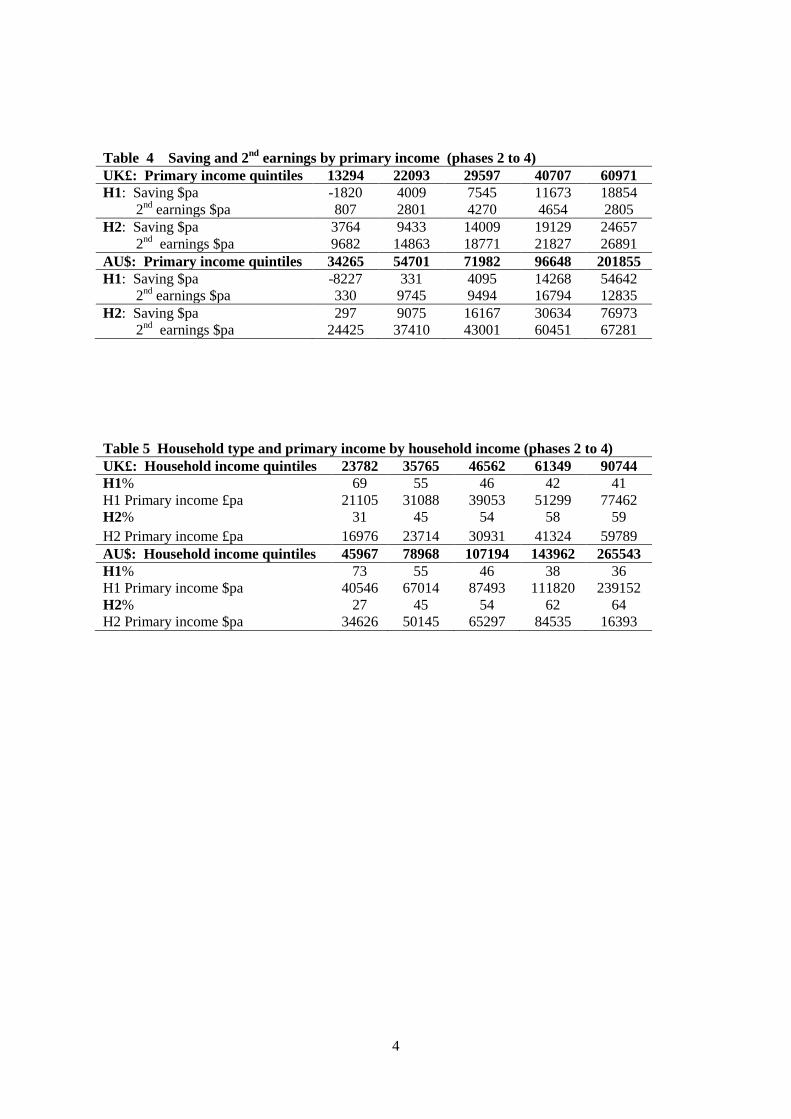
3.4 Saving and second income

The data indicate that household saving tends to track within-phase femalelabour supply because it tracks the second income. This becomes evident whenwe rank households in phases 2 to 4, partitioned as described for Table 2, byquintiles of primary income and then partition the records in each quintile intotwo household types:Type H1: Second earner working at or below median second worker hours;Type H2: Second earner working above median second worker hours.Table 4 reports predicted levels of saving by household type, H1 and H2,

based on regression estimates that control for the number and age of children.The table also gives the data means for second earnings. It can be seen that thelevel of saving depends heavily on the contribution made by the second earneracross the middle quintiles of the distribution.Table 4 hereThese results suggest that the labour supply effects of high effective tax rates

on the second earner may have a very significant negative effect on saving, farmore so than a tax on saving directly or a tax on capital income. Female labouris arguably the most mobile factor of production in the economy, because ofits high degree of substitutability with household production, especially in theform of parental child care in the early phases of the life cycle. OECD countrieswith family tax and child support systems that do not discriminate as heavilyagainst the second earner have far higher female labour supplies, for example inthe order of 50% higher in the case of Sweden. The preceding analysis suggeststhat the same countries also will tend to have higher levels of saving (as opposedto saving rates) and greater taxing capacity for the purpose of public investmentin child care and education as a result of their larger tax base.

3.5 Welfare ranking errors

Defining household welfare on joint income can lead to serious ranking errorsdue not only to heterogeneity in child care choices but also to the shape of theprimary wage distribution. An important feature of primary income rankingsin countries such as the UK, US and Australia is a relatively flat profile acrossmuch of the distribution followed by a steep rise in the upper percentiles. Ina distribution of primary income of this shape, the position of a family in ahousehold income ranking will be very sensitive to the labour supply of thesecond earner, because it will take only a small increase in her earnings toshift the family to a significantly higher point in the distribution. In a primaryincome ranking, households with the second earner working full time tend to berelatively evenly distributed across the distribution. In contrast, in a householdincome ranking they are much more strongly represented in the upper quintiles.This allows low wage families to be misrepresented as “high income” in the

have a large impact on female labour supply when home and market child care tend to besubstitutes. This is missed in studies that treat parental child care as leisure and bought-incare as a consumption good.

11

discussion of joint income tested family payments. To illustrate the problem,Table 5 compares rankings of the two household types, H1 and H2, by quintilesof household income for couples in phases 2 to 4 with a primary income of atleast £ 6,000 in the ONS LCF sample and of $10,000 in ABS HES sample.Table 5 hereIn the UK distribution the upper income limit of quintile 1 is £ 30,628 and

the lower income limit of quintile 4 is £ 52,988. A single-earner family on anannual income of £ 28,000 will be located in quintile 1. If the family switches"type", with the second earner taking up full time employment for the sameincome, the family will be re-ranked from quintile 1 to quintile 4.The potential for reranking of low wage families when a second partner goes

out to work is just as high in the Australian distribution. The correspondingincome limits are $67,288 and $125,372. A single-earner family on an incomeof $63,000 will move to quintile 4 if the second partner earns the same income.If the family has a preschool child, much of the second net income may bespent on child care and associated cost of entering the workforce. Clearly, sucha household cannot be said to have the same standard of living as another inwhich only one parent needs to work full time to earn $126,000 while the otherworks full time at home.28 These are the underlying assumptions in argumentsthat identify household utility possibilities with household income.

4 A tax reform analysis

Much, though by no means all, of the discussion of income and expendituretaxation in the chapters under review proceeds as if households consisted ofindividual worker/consumers. In those relatively brief sections in which thereality of family taxation is allowed to intrude, the discussion of earnings tax-ation seems obsessed by an old29 but not very significant conundrum. This ispresented as follows:30

"To be neutral with respect to whether two individuals form a couple or not,the tax and benefit system would have to treat them as separate units. But totreat all couples with the same combined income equally, the tax and benefitsystem would have to treat couples as a single unit. If an individualized systemis progressive, so that the average tax rate rises with income, then two coupleswith identical joint incomes but different individual incomes would pay differentamounts of tax.[...] A tax system cannot simultaneously be progressive, neutraltowards marriage/cohabitation, and tax all families with the same joint incomeequally."

28 In Apps and Rees (2012) we show that when home and market child care tend to besubstitutes - a plausible assumption for the UK and Australia given the state of their childcare sectors - small variations in price that have little effect on household utility on cangenerate wide variation in second earner labour supplies. Under these conditions we showthat progressive individual taxation with universal family payments is optimal.29See Rosen (1977).30Op.cit. p 66.

12

The review appears to use the existence of this dilemma as a reason for notaccepting the superiority of individual over joint taxation, despite the weight oftheoretical and empirical work supporting this, and to retain, in its proposalsfor the UK tax system, the elements of joint taxation in what is supposedly anindividual tax system in the UK.However, this supposed dilemma is an entirely false one. Horizontal equity,

defined as the imposition of equal tax burdens on households with equal ca-pacities to generate utility for their members, is not served by equalising taxburdens on households with equal incomes, since, as just pointed out, in realityhousehold income is not a good or reliable measure of the household’s utilitypossibilities. Having tax burdens that vary across households with equal jointincomes in a way determined by optimal individual taxation does less damageto horizontal equity than joint taxation, and removes the basis of the case forretaining the elements of joint taxation in the UK tax system.31 A stronglyprogressive individual-based income tax with universal family payments can beexpected to contribute to a greater degree of vertical and horizontal equity, es-pecially given the current distribution of primary incomes and the potential forerrors in a welfare ranking defined on household income of the order of magni-tude we have just demonstrated.Interestingly, in the light of our comments above on the underlying view of

the life cycle the review appears to take, it does advocate reducing the tax bur-den on families with school age children, though apparently funding this at leastin part by raising that on families with preschool children.32 Citing evidencethat the elasticity for employment of single mothers is 0.85 when their youngestchild is aged at least five, as compared to around 0.5 for those with youngerchildren, they base this proposal on the greater reponsiveness to incentives ofthe former group. Though we welcome the more realistic view of the life cycleunderlying this recommendation, we would argue that it gets things preciselythe wrong way around. The reason for the relatively lower (but still high bycomparison with elasticities of male labour supply) responsiveness for mothers ofpre-school aged children is of course the constraints they face in obtaining goodquality child care at affordable prices. The cost of reduced labour supply at thisstage in the life cycle is likely to be a loss of human capital and worsened futureemployment possibilities. Thus reductions in marginal tax rates of secondaryearners with pre-school children, together with expenditure on improving childcare facilities, is likely to have a more productive effect on labour supply, in theshort and longer term, than the policy proposed by the review.

4.1 Integrating capital and labour income taxation

A notable omission in the review is the integration of the proposal for the taxtreatment of capital income, which, as we pointed out above, necessarily involvesjoint taxation, with the system of labour earnings taxation, which is taken to be

31See Apps and Rees (2012), which analyses this issue in some depth.32See pages 111-115 of the review.

13

based on individual incomes. To explore this issue we take a household with twoearners facing an individual-based, piecewise linear progressive labour earningstax system, and first consider what happens to their budget constraint undereach of the three forms of expenditure taxation considered by the review and setout above. We then go on to carry out a tax reform analysis of the proposal inthe review to introduce a "rate of return allowance" in an economy in which, asjust discussed, household income and utility possibilities are not co-monotonic.Throughout, we use a to denote a lump sum transfer under the tax system,33

ti the marginal tax rate paid by individual34 i = 1, 2 on individual income yi, sis household saving, τ the tax rate on the income from saving yielding a rate ofreturn r in the second period, and x1, x2 are total household consumptions inperiods 1 and 2 respectively. The household works, consumes and saves in thefirst period and consumes the income from its saving in the second.

4.1.1 EET

Under individual taxation it is necessary to specify exactly how the exemptionfrom taxation of income that is saved is given. We assume that some proportionki ∈ [0, 1] of total saving is set against the labour income of individual i = 1, 2,with

∑i ki = 1. In the simplest case of a two-period model in which individuals

work, consume and save in the first period and consume the net proceeds ofsaving in the second, we have the single period budget constraints as

x1 + s ≤ a+∑i

[yi − ti(yi − kis)] (1)

x2 ≤ (1− τ)(1 + r)s (2)

yielding the wealth constraint

x1 +1−

∑i kiti

(1− τ)(1 + r)x2 ≤ a+∑i

(1− ti)yi (3)

Then clearly the saving decision is undistorted relative to the situation withouta savings tax if and only if

∑i kiti = τ . If the household is allowed to set all its

saving against the income of the primary (by assumption more highly taxed)earner, k1 = 1, then this could represent an implicit subsidy to saving.35

33Strictly we should write the budget constraint as x1 ≤ a+∑i(1− ti)yi +(t1− t2)y, where

y is the upper limit of the lower tax bracket, but we can regard the term (t1 − t2)y as beingsubsumed in a.34For simplicity we assume that all primary earners pay the higher marginal tax rate t1 and

all second earners the lower marginal tax rate t2. In reality of course households may consistof two high wage/high tax rate or two low wage/low tax rate individuals. This assumptionhowever suffi ces to allow us to make the main points.35The review of course stresses that the neutrality result may fail to hold when the household

faces different marginal tax rates in the first and second periods. In this particular case theneed to raise tax revenue might require ceilings on the value of s.

14

4.1.2 TEE

The wealth constraint in this case is

x1 +1

(1 + r)x2 ≤ a+

∑i

(1− ti)yi (4)

and saving is clearly undistorted. However, a revenue neutral change from asituation in which capital income was taxed would of course require an increasein labour earnings taxation and increased distortion of labour supplies.

4.1.3 TtE

This proceeds by defining a "normal rate of return" rN and an "excess return"ρ = max[0, r − rN ], where r is again the realised rate of return. The singleperiod budget constraints are then

x1 + s ≤ a+∑i

(1− ti)yi (5)

x2 ≤ (1 + r − τρ)s (6)

The wealth constraint is then

x1 +1

1 + r − τρx2 ≤ a+∑i

(1− ti)yi (7)

If the review intends rN to be the rate of return at which saving in the economyis in some sense optimal, then as long as the tax rate τ < 1 and the "excessrate of return" ρ > 0, there will still be "too much" saving. Obviously TEEand TtE are equivalent if ρ = 0, the actual rate does not exceed the normalrate. If on the other hand ρ = r so that the normal rate is effectively zero, wehave the full taxation of capital income. Thus a marginal reduction in capitalincome taxation following from increasing the allowed rate of return rN impliesdρ < 0.Since the TtE system is the main innovation proposed in the review, we

carry out our tax reform analysis on the assumption that this is the alternativeto the full taxation of the income from saving, i.e. the non-exemption of the"normal rate of return".

4.2 The tax reform model

The intuition of the results we derive in the following formal analysis is quitestraightforward, though they may seem counter-intuitive if one’s intuition isbased only on the model of the household as a single individual.To ensure revenue neutrality of the reduction in taxation on the income from

saving, we have to increase earnings taxation.36 Since a reduction in the lump

36Alternatively of course the government could increase indirect taxation, reduce expendi-ture or increase borrowing. We do not consider these possibilities here.

15

sum a is obviously regressive, while the review generally rules out an increase inthe higher rate of income tax, here t1, we have to increase the lower tax rate t2to maintain tax revenue. This, in the framework we have here, means increasingtaxation of second earners.37 This makes the corresponding households worseoff as long as the relationship between second earner income and their savingsatisfies a reasonable condition given below, which implies that they benefitfrom the saving tax reduction by an amount less than the cost to them of theincome tax increase. Their saving may also fall, even if we assume, as does thereview, that the substitution effect of a change in the tax on saving outweighsthe income effect of that change. The reason for this is of course that the fall intheir labour earnings after the increase in t2 gives an additional income effectwhich will reduce consumption in all periods. This therefore reduces the increasein saving following the fall in the savings tax rate and may even make it negativein the aggregate. Households with saving that is high relative to second earner’sincome will be better off. Overall however social welfare may fall if householdwelfare is not monotonically increasing with joint income and if second earnerlabour supply elasticities with respect to earnings tax rates are high relative tothe elasticity of saving with respect to the saving tax rate.We assume two types of households, indexed h = 1, 2, with utility functions

Uh = u1h(x1h − ψ1h(y1h)− ψ2h(y2h)) + u2h(x2h) (8)

The form of the utility function rules out income effects on earnings but allowsthem on both current and future consumption. The household subscripts shouldnot be thought of as denoting a simple difference in preferences, but rather asdenoting reduced form functions that reflect such factors as differences in pro-ductivity in household production and in prices of bought-in child care leadingto differences in choices of second earner labour supply. In particular we assumey21 > y22 = 0. Given the budget constraints for this case in (5) and (6) above,we simplify the model by writing the period 2 utility as u2h(π(ρ)sh), whereπ(ρ) ≡ (1 + r − τρ) > 1 is the marginal net of tax return to saving.It is straightforward to show that the household optimisation implies supply

functions for earnings given by yih(ti), which involve no income effects, and de-mand functions for first period consumption and saving given by x1h(π(ρ), Yh),sh(π(ρ), Yh), where Yh = a+

∑i(1− ti)yih(ti) is first period disposable income.

Note that the tax rates on earnings affect consumption and saving only throughtheir effects on disposable income as a result of the assumed form of the utilityfunction.We are going to take as the two variable policy instruments t2 and ρ (equiv-

alently rN ), while holding r, τ and t1 fixed. In the usual way we can defineindirect utility functions vh(t2, π(ρ)), with derivatives

∂v1∂t2

= −λ1y21(t2);∂vh∂ρ

= −λhτsh/π(ρ) h = 1, 2 (9)

37 In reality, low wage primary earners will also be among these, but given assortative match-ing, this will strengthen the distributional aspects of the following discussion.

16

where λh is the marginal utility of household income and recalling that ∂v2/∂t2 ≡0 by assumption.The government budget constraint is∑

h

φh[t1y1h + t2y2h + τρsh]− a ≥ G (10)

where φh is the proportion of type h households in the population,∑h φh = 1,

and G ≥ 0 is a per capita revenue requirement. It follows that revenue neutralityrequires

dt2 = −µdρ (11)

where

µ ≡∑h φhτsh(1 + ε

sρh )

φ1[y21(1 + εy21t21 ) + τρ ∂s1∂Y1

∂Y1∂t2]> 0 (12)

Here εshρh , εy21t21 are elasticities and the sign restriction reflects the assumptionthat taxation is effi cient, in the sense that reducing one tax must result in anincrease in the other. Note that the second term in brackets in the denominatoris negative, since saving is increasing in household income which is decreasingin the tax rate t2.

Turning now to an analysis of the welfare effects, we assume a utilitariansocial welfare function

W =∑h

φhvh((t2, π(ρ)) (13)

giving

dW =∑h

φh[∂vh∂t2

dt2 +∂vh∂π

π′(ρ)dρ] (14)

= [φ1λ1(µy2h −τ

πs1)− φ2λ2

τ

πs2]dρ (15)

Since dρ < 0, we require the term in square brackets to be negative for anincrease in welfare to follow from a reduction in the taxation of the return fromsaving, but the first term in these brackets will be positive if y2h satisfies thecondition

y2h >τ

πµs1 (16)

and so the welfare effect of the policy change could be negative overall if

(µy2h −τ

πs1) >

φ2λ2φ1λ1

τ

πs2 (17)

in line with the intuition given above. This simply says that the welfare loss tothe households that lose from the tax policy outweighs the benefit to those thatgain.Aggregate saving falls if

−µφ1τ

∂s1∂Y1

∂Y1∂t2

>∑h

φh∂sh∂π

(18)

17

which simply says that the negative effect on saving of the increase in earningstaxation outweighs the positive effect of the reduction in capital income taxationin absolute value. A priori there is nothing to rule out satisfaction of thiscondition and as far as we know there is no empirical evidence to suggest thatit could not be satisfied.

5 Conclusions

This paper has provided a critique of the review’s main proposals on the taxa-tion of the income from household saving that is based on taking a fundamen-tally different view of the household than that which underlies the argumentspresented to support those proposals. We believe that this view supports a dif-ferent approach, that of finding the second best optimal taxation for both typesof income, where neither can be expected to have a zero optimal tax rate. In fol-lowing this approach, it is essential in our view to use models that take accountof the real characteristics of the household, as we have sought to describe themin this paper. Also, the problem should be formulated as that of finding theoptimal parameters of a tax system that is based on individual labour incomesand a piecewise linear system of marginal tax rates applied to these. Whetherthe tax on capital income should be also piecewise linear or a flat rate tax38 is anopen question a priori, that can and should be analysed within this framework.

References

[1] Alesina, A, A Ichino and L Karabarbounis (2007), Gender Based Taxationand the Division of Family Chores, Harvard University Discussion Paper.

[2] Apps, P, NV Long and R Rees (2011), Optimal Piecewise Lin-ear Income Taxation, IZA Discussion Paper No 6007. Available at:http://ftp.iza.org./dp6007.pdf

[3] Apps, P and R Rees (2009), Public Economics and the Household, Cam-bridge: Cambridge University Press.2010

[4] Apps, P and R Rees (2010),Family Labour Supply, Tax-ation and Saving in an Imperfect Capital Market, Reviewof Economics of the Household, 8, 297-323. Available at:http://www.springerlink.com/openurl.asp?genre=article&id=doi:10.1007/s11150-010-9094-1

[5] Apps, P and R Rees (2011), “Household Time Use, Inequality and Taxa-tion”, in JA Molina (ed), Household Economic Behaviors, Springer: NewYork (2011), Ch 3, 57-81.

38As in the "dual income tax system".

18

[6] Apps, P and R Rees (2012), Optimal Taxation, Child Care and Models ofthe Household", mimeo.

[7] Atkinson, A and J Stiglitz (1976), The Design of Tax Structure: Direct vsIndirect Taxation, Journal of Public Economics, 61, 55-75.

[8] Auerbach, A (2009), Choice Between Income and Consumption Taxes: APrimer, in A Auerbach and D Shaviro (eds), Institutional Foundations ofPublic Finance: Economic and Legal Perspectives, Cambridge, MA: MITPress

[9] Australia’s Future Tax System Review Panel (2009), Australia’s Future TaxSystem: Report to the Treasurer (Henry Review).

[10] Banks, J and P Diamond (2008),The Base for Direct Taxation, DiscussionPaper submitted to the Mirrlees Commission on Tax Reform.

[11] Banks, J and P Diamond (2010),The Base for Direct Taxation, in Mirrleeset. al., (2010), Dimensions of Tax Design, Oxford University Press.

[12] Boskin, MJ and E Sheshinski, (1983), Optimal Tax Treatment of the Fam-ily: Married Couples, Journal of Public Economics, 20, 281-297.

[13] Chamley, C (1986), Optimal Taxation of Capital Income in General Equi-librium with Infinite Lives, Econometrica 54(3), 607-22

[14] Corlett, WJ, and DC Hague (1953), "Complementarity and the ExcessBurden of Taxation, Review of Economic Studies, 21, 21-30.

[15] Judd, K (1985), Redistributive Taxation in a Simple Perfect ForesightModel, Journal of Public Economics, 28(1), 59-83.

[16] Meade, J (1978), The Structure and Reform of Direct Taxation: Report ofa Committee chaired by Professor J E meade, London: George Allen andUnwin

[17] Mirrlees, J, S Adam, T Besley, R Blundell, S Bond, R Chote, M Gammie,P Johnson, G Myles, J Poterba (2010), Dimensions of Tax Design, OxfordUniversity Press.

[18] Mirrlees, J, S Adam, T Besley, R Blundell, S Bond, R Chote, M Gammie,P Johnson, G Myles, J Poterba (2011), Tax by Design, Oxford UniversityPress.

[19] Munnell, A (1980), The Couple versus the Individual under the FederalPersonal Income Tax, in H Aaron and M Boskin (eds),The Economics ofTaxation, The Brookings Institution, 247-280.

[20] H Rosen, H (1977), Is It Time to Abandon Joint Filing, National TaxJournal, XXX, 423-428.

19

[21] Sørenson, PB (2005), Neutral Taxation of Shareholder Income, Interna-tional Tax and Public Finance, 12, 777-801.

20

1

Table 1 Life cycle time use, hours pa Male hours Female hours

Phase Market Domestic Child care Market Domestic Child care UK

1 1762 745 - 1457 1027 - 2 1855 718 769 674 1291 1693 3 1768 836 267 1019 1427 561 4 1556 866 - 906 1465 - 5 323 1219 - 156 1627 -

AU 1 1857 753 - 1508 1047 - 2 1985 747 1221 532 1471 2250 3 1845 897 434 934 1671 716 4 1558 909 - 807 1624 - 5 381 1228 - 129 1241 -

Figure 1 Life cycle time use, hours pa

(a) UK time use (b) AU time use

010

0020

0030

00

Mark

et h

ours

pa

1 2 3 4 5Life cycle phase

Male mkt hrs Female mkt hrs

010

0020

0030

0040

00

Dom

estic

and

chi

ld c

are

hour

s pa

1 2 3 4 5Life cycle phase

Male dom+cc hrs Female dom+cc hrsMale dom hrs Female dom hrs

010

0020

0030

00

Mar

ket h

ours

pa

1 2 3 4 5Life cycle phase

Male mkt hrs Female mkt hrs

010

0020

0030

0040

00

Dom

estic

and

chi

ld c

are

hour

s pa

1 2 3 4 5Life cycle phase

Male dom+cc hrs Female dom+cc hrsMale dom hrs Female dom hrs

2

Table 2 Median incomes, earnings and saving, 2010

Phase Household

income Female

earnings Disposable

Income

Saving UK£

1 47996 19994 37960 13676 2 35152 6604 32110 8892 3 42588 8970 39468 9620 4 39468 10972 31720 8320 5 12756 0 22932 3224 AU$

1 116141 47502 96122 19760 2 83824 6240 80236 5824 3 110244 30212 93964 9776 4 94744 26208 83252 14040 5 6980 0 33956 1404

Table 3 Employment status by gender, 2010

Phase Males Females

FT PT NE FT PT NE UK

1 86.9 4.4 8.7 78.2 11.1 10.6. 2 79.2 8.4 12.4 21.8 44.5 33.6 3 80.9 8.1 10.9 32.2 44.0 23.8 4 74.6 8.8 16.6 42.3 30.9 26.9 5 15.5 10.1 74.4 4.9 14.2 80.8

AU 1 88.9 8.5 2.6 72.5 18.2 9.3 2 90.3 5.5 4.2 18.4 37.5 44.1 3 86.2 7.3 6.5 36.2 44.8 19.0 4 78.3 9.9 11.8 35.3 35.9 28.8 5 16.5 10.3 73.2 6.9 12.9 80.2

3

Figure 2 Employment status by gender

UK employment status by gender: phases 1 to 4

020

4060

8010

0Fr

eque

ncy

%

0 hrs 1-34 hrs 35+ hrs

Phase 4: Post-children

Males Females

020

4060

8010

0Fr

eque

ncy

%

0 hrs 1-34 hrs 35+ hrs

Phase 1: Pre-children

Males Females

020

4060

8010

0Fr

eque

ncy

%

0 hrs 1-34 hrs 35+ hrs

Phase 2: Child 0-4

Males Females

020

4060

8010

0Fr

eque

ncy

%

0 hrs 1-34 hrs 35+ hrs

Phase 3: Child 5+

Males Females

AU employment status by gender: phases 1 to 4

020

4060

8010

0Fr

eque

ncy

%

0 1-34 35+

Phase 2: Child 0-4

Males Females

020

4060

8010

0Fr

eque

ncy

%

0 hrs 1-34 hrs 35+ hrs

Phase 4: Post-children

Males Females

020

4060

8010

0Fr

eque

ncy

%

0 hrs 1-34 hrs 35+ hrs

Phase 1: Pre-children

Males Females

020

4060

8010

0Fr

eque

ncy

%

0 hrs 1-34 hrs 35+ hrs

Phase 2: Child 0-4

Males Females

020

4060

8010

0Fr

eque

ncy

%

0 hrs 1-34 hrs 35+ hrs

Phase 3: Child 5+

Males Females

4

Table 4 Saving and 2nd earnings by primary income (phases 2 to 4) UK£: Primary income quintiles 13294 22093 29597 40707 60971 H1: Saving $pa -1820 4009 7545 11673 18854 2nd earnings $pa 807 2801 4270 4654 2805 H2: Saving $pa 3764 9433 14009 19129 24657 2nd earnings $pa 9682 14863 18771 21827 26891 AU$: Primary income quintiles 34265 54701 71982 96648 201855 H1: Saving $pa -8227 331 4095 14268 54642 2nd earnings $pa 330 9745 9494 16794 12835 H2: Saving $pa 297 9075 16167 30634 76973 2nd earnings $pa 24425 37410 43001 60451 67281

Table 5 Household type and primary income by household income (phases 2 to 4) UK£: Household income quintiles 23782 35765 46562 61349 90744 H1% 69 55 46 42 41 H1 Primary income £pa 21105 31088 39053 51299 77462 H2% 31 45 54 58 59 H2 Primary income £pa 16976 23714 30931 41324 59789 AU$: Household income quintiles 45967 78968 107194 143962 265543 H1% 73 55 46 38 36 H1 Primary income $pa 40546 67014 87493 111820 239152 H2% 27 45 54 62 64 H2 Primary income $pa 34626 50145 65297 84535 16393