1 Capital Inflow Shocks and House Prices: Aggregate and Regional Evidence from Korea Peter Tillmann 1 Justus‐Liebig‐University Giessen February 2013 This paper also appeared as Bank of Korea Working Paper 2013‐2. Abstract Over the course of the recent global financial crisis, emerging economies experienced massive swings in capital inflows. In this paper, we estimate a VAR model to assess the impact of capital inflow shocks, which are identified using a set of sign restrictions, on house prices in Korea. We base the analysis on three alternative measures of capital inflows: net total inflows, net portfolio inflows and gross total inflows. The results suggest that capital inflow shocks have a significantly positive and persistent effect on real house prices. Although shocks to capital inflows are found to be substantially more important for Korean asset markets than for other OECD countries, their overall explanatory power is modest. Using regional house price data we also show that capital inflow shocks have an asymmetric effect on property markets across the seven largest Korean cities and across different parts of Seoul. Keywords: Capital Inflows, House Prices, Monetary Policy, Sign Restrictions, VAR JEL classification: F32, F41, E32 1 This paper was written while I enjoyed the generous hospitality of the Bank of Korea’s Economic Research Institute. I thank Junhan Kim for providing some of the data and seminar participants at the Bank of Korea for many insightful discussions. An anonymous referee of the Bank of Korea’s working paper series provided very helpful comments. Contact: Department of Economics, Justus‐Liebig‐ University Giessen, Licher Str. 66, 35394 Giessen, Germany, Email: [email protected].
Transcript
1
Capital Inflow Shocks and House Prices:
Aggregate and Regional Evidence from Korea
Peter Tillmann1
Justus‐Liebig‐University Giessen
February 2013
This paper also appeared as Bank of Korea Working Paper 2013‐2.
Abstract
Over the course of the recent global financial crisis, emerging economies experienced
massive swings in capital inflows. In this paper, we estimate a VAR model to assess the
impact of capital inflow shocks, which are identified using a set of sign restrictions, on
house prices in Korea. We base the analysis on three alternative measures of capital
inflows: net total inflows, net portfolio inflows and gross total inflows. The results
suggest that capital inflow shocks have a significantly positive and persistent effect on
real house prices. Although shocks to capital inflows are found to be substantially more
important for Korean asset markets than for other OECD countries, their overall
explanatory power is modest. Using regional house price data we also show that capital
inflow shocks have an asymmetric effect on property markets across the seven largest
Korean cities and across different parts of Seoul.
Keywords: Capital Inflows, House Prices, Monetary Policy, Sign Restrictions, VAR
JEL classification: F32, F41, E32
1 This paper was written while I enjoyed the generous hospitality of the Bank of Korea’s Economic
Research Institute. I thank Junhan Kim for providing some of the data and seminar participants at the
Bank of Korea for many insightful discussions. An anonymous referee of the Bank of Korea’s working
paper series provided very helpful comments. Contact: Department of Economics, Justus‐Liebig‐
University Giessen, Licher Str. 66, 35394 Giessen, Germany, Email: [email protected].
2
1. Introduction
The recent financial crisis in many industrial economies was reflected in massive swings
in international capital flows to emerging market economies. 2 In particular, cross‐border
flows to emerging economies exhibited again the boom‐bust pattern that resembles
previous financial crises. A dramatic withdrawal of international investments by global
investors following the Lehman collapse in 2008 was followed by a quick and
voluminous return of capital flows in 2009 when ultra‐loose monetary conditions in the
US and other economies and the resulting yield differential pushed capital back to
emerging market economies.
In his account of the recent unconventional monetary measures taken by the US Federal
Reserve and their impact on capital flows, Morgan (2011) argues that about 40% of the
increase in the US monetary base under QE1 eventually resulted in increased gross
capital outflows. With their relatively solid macroeconomic and financial development,
Asian economies, much more than e.g. countries in Latin America or Emerging Europe,
received the bulk of these flows. 3
A common concern is that the abundance of global liquidity results in massive capital
inflows that pose risks to financial stability in the receiving countries as flows increase
domestic liquidity and might fuel asset price bubbles.4 Chen et al. (2012), among others,
argue that the recent rounds of Quantitative Easing were associated with spillover
effects boosting asset prices globally. Given their crucial role in the monetary
transmission mechanism and its contribution to financial stability, the consequences of
capital inflows driven by global push‐factors for housing markets are particularly
relevant.5
In this paper we analyze the impact of capital inflow on house prices and equity prices,
taking Korea as an example. For that purpose, we estimate a VAR model to gauge the
dynamic effects of capital inflow shocks. A reduced‐form VAR approach is well suited
to quantify the effect of capital inflows as it is consistent with a wide range of economic
models. Moreover, given that various transmission channels between capital inflows
and asset prices coexist, applying a VAR model delivers results that do not hinge on just
one transmission channel. In fact, capital inflows extend domestic saving and will thus 2 The dynamics of global capital flows during the recent financial crisis are studied in Milesi‐Ferretti and
Tille (2011), Forbes and Warnock (2011) and Förster, Jorra and Tillmann (2012). 3 The development of capital flows to Asia during the financial crisis is analyzed by IMF (2011 a,b) and
Tille (2011). 4 Bernanke (2010) explicitly links capital flows to house price bubbles. 5 The determinants of property prices in Asian economies are studies by Zhu (2006) and Glindro et al.
(2011). Kim (2004) surveys the role of housing for the Korean economy.
3
lead to an expansion of credit to households and firms. A rapid expansion of credit will
eventually become unsustainable. Domestic financial institutions which have access to
abundant liquidity, might lend excessively to property markets. In addition, cheap
global liquidity together with unusually low interest rates in industrial countries will
provoke a search‐for‐yield behavior were investors take on higher risks in emerging
economies’ asset markets.
The identification of capital inflow shocks is not trivial as in small open economies many
macroeconomic shocks typically result in capital movements across borders. Thus, we
have to carefully identify capital inflow shocks. In this paper, we employ sign
restrictions as proposed by Sá, Towbin and Wieladek (2011) to identify exogenous
shocks to foreigners’ demand for domestic assets, i.e. capital inflow shocks. Our notion
of capital flow shocks corresponds to capital flows driven by push‐factors such as
monetary policy in advanced economies or global risk aversion.
We base the analysis on three alternative measures of capital inflows, net total inflows,
net portfolio inflows and gross total inflows. The results suggest that capital inflow
shocks have a significantly positive and persistent effect on real house prices. Shocks to
capital inflows are found to be substantially more important for Korean asset markets
than for other OECD countries.
In a companion paper, see Tillmann (2012), we use that identification scheme to analyze
capital flow shocks in a panel of Asian economies. Besides focusing on the Korean case,
this paper also allows for a second novelty. As a key contribution, we evaluate the
extent to which the sensitivity of house prices to capital inflow shocks differs across
Korean cities. Put differently, we ask whether the results obtained from nation‐wide
house price data is informative for major metropolitan regions. Using regional house
price data we show that capital inflow shocks have an asymmetric effect on property
markets across the seven largest Korean cities and across the northern and the southern
half of Seoul, respectively. This result suggests that macroprudential policy measure
might be best suitable to curb the impact of inflows on asset prices as these measures
can be tailored to regional housing markets.6
The remainder of the paper is organized as follows: Section two connects the paper to
different strands of the literature. The VAR model and the data set are introduced in
section three. Section four discussed the identification of capital inflows shocks. The
6 For a survey on macroprudential measures see Crowe et al. (2011), Pradhan et al. (2011) and Ostry et al.
(2011). The policy responses to capital inflows taken by Korean authorities are sketched in Chung (2010).
4
main results, including a set of robustness checks, are presented in section five. In
section six we evaluate whether the sensitivity of house prices to capital inflows differs
across major Korean cities. The final section draws conclusions.
2. Related literature
A number of papers address the connection between capital inflows and asset market
developments. In this literature, the VAR approach, either on an individual country
basis as in this paper or in a panel set‐up, takes center stage. In the following we briefly
related this paper to the available literature.
The paper draws heavily on Tillmann (2012), who in turn uses the identification
approach of Sá, Towbin and Wieladek (2011) to estimate the effect of capital inflow
shocks in a panel of economies from emerging Asia in the post‐1999 period. The key
contribution of these papers is to use sign restrictions to identify capital inflow shocks in
an otherwise standard VAR model. The identification via sign restrictions avoids the
need to impose an often arbitrary ordering onto the variables which plagues the
identification using the well‐known Cholesky decomposition. Such a triangular
identification scheme requires that the direction of causality between capital inflows,
monetary policy responses and asset price movements within a given quarter to be
restricted ex ante. Given the complex nature of the macroeconomic relationships and
responses involved, this approach is often considered arbitrary. Tillmann (2012) finds
that capital inflows have a significantly positive impact on house prices and account for
a fraction of house price changes that is twice as large as in OECD countries. While a
panel approach has its virtues in light of the short sample period available after the
disruptions of the Asian financial crisis, it cannot shed light on country‐specific
developments. This paper closes this gap and uses a similar approach to study capital
inflows to Korea.
Kim and Yang (2009) present a similar exercise within a more conventional, recursively
identified VAR model, which suffers from the problem of imposing an arbitrary
ordering of the variables as discussed before. They show that capital inflow shocks have
a significantly positive impact on Korean stock prices but not on house prices. When the
capital flow measure is narrowed to include only portfolio flows, the impulse response
remains insignificant. Kim and Yang (2011) adopt the same approach to a panel VAR
estimated on five Asian economies. It turns out that capital flow shocks explain only a
small portion of asset price fluctuations.
A related strand of the literature studies the sensitivity of house prices to monetary
policy shocks. Prominent contributions include Assenmacher‐Wesche and Gerlach
(2008) and Goodhart and Hofmann (2008), who estimate panel VARs on OECD
5
countries to show that monetary policy shocks have a significant effect on asset prices.
Bracke and Fidora (2008) focus on the asset price responses in Asian emerging
economies. He identifies monetary policy shocks using sign restrictions, but aggregate
individual economies using GDP weights. Monetary policy shocks are shown to explain
a large part of asset price fluctuations. The studies of Vargas‐Silva (2008), Mallick and
Sousa (2011), Carstensen, Hülsewig and Wollmershäuser (2009) and Hristov, Hülsewig
and Wollmershäuser (2011) provide VAR evidence, derived from country‐specific or
panels, on the impact of monetary policy shocks. These papers, however, do not address
capital inflow shocks and do not cover Asian economies, respectively.
A separate branch of the literature focuses on the relationship between the (negative)
current account balance as a measure of capital inflows and various asset markets.
Fratzscher, Juvenal and Sarno (2010) use a VAR with a sign‐restriction identification
scheme to assess the impact of asset market shocks on the U.S. current account.
Reduced‐form evidence on the relationship between asset prices and the current account
balance typically finds a robust negative correlation between the growth rate of house
prices and the change in a countryʹs current account balance, see e.g. Kole and Martin
(2009), Aizenman and Jinjarak (2009), Adam, Kuang and Marcet (2012), Jinjarak and
Sheffrin (2011) and Kannan, Rabanal and Scott (2011).
3. The VAR approach
Since the present paper is not a contribution to the methodology, we do not present the
full details of the estimation and identification procedure. The interested reader is
refereed to Uhlig (2005) and Fratzscher, Juvenal and Sarno (2010) for thorough
expositions. Here we give only the gist of the of the sign restrictions approach.
The estimated VAR model of order q takes the form
q
ititit uYBBY
10 ,
where tY is an 1m vector of observables, iB are mm coefficient matrices and tu is the
vector of one‐step ahead prediction errors with a variance‐covariance matrix . The
vector 0B collects the intercept terms.
To recover the structural shocks tv behind the reduced form residuals, the restrictions
emerging from the covariance structure are not sufficient. In addition, we follow Uhligʹs
(2005) seminal (pure) sign‐restrictions approach. As mentioned before, standard VARs
are typically identified imposing restrictions on the contemporaneous relationships
among the variables. This is equivalent to imposing a recursive ordering onto the
variables in tY .
6
Table 1: The identifying restrictions
Variable in the VAR Impact of capital inflow
shock
Horizon
Capital inflows + 3 quarters
Output + 3 quarters
Price level unrestricted
Asset prices unrestricted
REER appreciation
Long rate
+
‐
3 quarters
3 quarters
Short rate unrestricted
Table 2: Lag order selection
Lag order AIC SIC HQ
0q 33.546 33.819 33.649
1q 18.884 21.067 19.709
2q 19.905 22.999 20.452
3q 17.942 23.945 20.210
4q 17.436 25.349 20.426
Here, the identification is achieved by imposing restrictions on the sign of the impulse
responses of the endogenous variables following the seminal contribution of Uhlig
(2005). He shows that an impulse vector can be recovered by combining 1n draws from
the VAR posterior and 2n draws from an independent uniform prior. We stop after
obtaining 3n impulse response functions with the desired sign over a horizonK . The
error bands are calculated using the draws kept. We set 200021 nn and 10003 n .
The VAR contains seven quarterly data series: net capital inflows in percent of GDP
( tFLOWS ), log real GDP ( tGDP ), the log consumer price index ( P ), the log real effective
7
exchange rate ( tREER ), a log real asset price ( tASSET ), the long‐term bond yield
( tLONG ) and the short‐term money market interest rate typically used to proxy the
Bank of Korea’s monetary policy stance ( tSHORT ). All variables enter the VAR in levels.
Hence, the vector of observations is
tttttttt SHORTLONGASSETREERPGDPFLOWSY ,,,,,,' .
In the benchmark specification, tFLOWS represent net total capital inflows defined as
the sum of foreign direct investment, portfolio inflows, derivatives inflows and other
types of inflows. Two alternative specifications substitute net total capital inflows by a
narrower measure covering only net portfolio inflows or gross total capital inflows.7
Moreover, in the benchmark specification tASSET stands for real (residential) house
prices. To compare the results, we also substitute real house prices by real equity prices.
A higher value of tREER means a real appreciation of the domestic exchange rate.
The macroeconomic data series and the stock price data are taken from the IMF’s
International Financial Statistics Database, the short‐term interest rate was provided by
the Bank of Korea, while the real effective exchange rate series and the series on house
prices are obtained from the BIS’s website.8 The estimation period starts in 1999:1, i.e.
after the disruptions caused by the Asian financial crisis, and ends in 2011:4. Estimating
the VAR model necessitates a choice of the lag order q . Table (2) presents three different
lag selection criteria, i.e. the Akaike criterion (AIC), the Schwarz information criterion
(SIC) and the Hannan‐Quinn information criterion (HQ). As so often, these three criteria
recommend different lag orders. While the SIC and the Q suggest to include just one lag,
the AIC, which puts much smaller weight on the loss of degrees of freedom once more
lags are included, signals the inclusion of up to four lags. We choose an intermediate
value and include two lags o the endogenous variables.
4. The identifying restrictions
The set of restrictions imposed in this paper is summarized in table (1). We interpret a
shock to net capital inflows as an exogenous, unexpected inflow of foreign capital
unrelated to domestic fundaments. Thus, capital inflow shocks can be thought of as
being the consequence of monetary policy and liquidity conditions in industrial
7 As discussed in Forbes and Warnock (2011), among others, “gross inflows” are “net” items reflecting the
difference between foreign purchases of domestic assets and foreign sales of domestic assets. Thus, gross
flows can also become negative. 8 The original IFS series report capital flows in USD. We convert these series to KRW using the nominal
exchange rate provided by the IFS and divide the result by nominal GDP.
8
countries, changes in global risk aversion of investors or contagion effects from other
countries.
To translate this notion of capital inflow shocks into our VAR model, this type of shocks
has to be distinguished from other shocks that would also eventually lead to an increase
in capital inflows. Shocks to domestic technology or domestic demand, for example,
would also attract foreign capital.
Here we adopt the identification scheme of Sá, Towbin and Wieladek (2011), which we
augment with a constraint on the output response as in Tillmann (2012). An
expansionary capital inflow shock is supposed to increase capital inflows, leads to an
increase in economic activity, puts appreciation pressure on the real effective exchange
rate and lowers long term interest rates. The restrictions are imposed for a horizon of
3K quarters.
We choose restrictions that are fairly non‐controversial in the literature on capital flows.
The restrictions used to identify capital inflow shocks are consistent with the empirical
findings of Cardarelli, Elekdag and Kose (2010), who conclude that shocks to capital
inflows have an expansionary effect on GDP and lead to a real appreciation. The
positive effect on output is also supported by Kim and Kim (2011) for a set of emerging
economies in Asia. The close association between capital inflows and appreciation
pressure on the domestic exchange rate is also documented by Jongwanich (2010) in a
dynamic panel model.
A key restriction is that on the long‐term interest rate. While other shocks such as a
positive technology shock or a demand shock would also lead to capital inflows, these
kinds of shocks would typically raise (real) interest rates. Thus, to distinguish a shock to
capital inflows stemming from an exogenous increase in foreigner’s demand for
domestic assets, probably caused by monetary policy in advanced economies, the
negative interest rate response imposed here is crucial.9 Again, this restriction is in line
with a large body of empirical evidence. Jongwanich (2010) shows that capital inflows
lower long‐term interest rates. Likewise, Pradhan et al. (2011) find that an increase in
nonresident participation in local bond markets by one percentage point reduces
nominal long‐term bond yields by about five basis points on average.
The response of real asset prices, i.e. either house prices or equity prices, is the central
focus of this paper. Consequently, we leave the asset price response unrestricted. Since
the asset price response to capital inflow shocks crucially depends on whether monetary
policy tightens or looses monetary conditions, we also leave the response of the short‐
term interest rate, i.e. the policy instrument of the Bank of Korea, unrestricted. Finally,
9 See Sá, Towbin and Wieladek (2011) for a detailed discussion of that issue.
9
the response of the price level is unrestricted to gauge the inflationary consequences of
sudden inflows of foreign capital.
5. Results
We first present the results from the specifications discussed in the previous sections.
After that, two modifications of the VAR specification are shown in order to corroborate
the robustness of the findings.
Impulse responses
The resulting impulse response functions are depicted in figure (1) to (6). All figures
show the response of the seven endogenous variables to a capital inflow shock one
standard deviation in size. The confidence bands are constructed using the 16th and 84th
percentiles of the accepted responses.
Figure (1) shows the baseline results obtained from a VAR with net total capital inflows
and house prices. A shock to capital inflows is associated with an increase in the inflows
to GDP ratio of about one percentage point. The shock leads to an expansionary effect
on output that outlasts the restricted response in the first three quarters. The same is
true of the real effective exchange rate, which significantly appreciates by two percent
for about seven quarters. Apparently, capital inflows do not have inflationary
consequences as the response of the CPI is essentially flat. Monetary policy as reflected
by the evolution of the short‐term interest rate tightens about three quarters after the
shock, although this response lacks empirical significance.
The response of house prices is the core empirical result of interest. Capital inflows
generate a significant house price boom which is associated with a persistent increase of
real house prices of about one percent for a period of five quarters.
The following figures show the corresponding impulse response functions for the
alternative VAR modifications. Most macroeconomic responses are similar to the
baseline specification. Figure (2) shows that once we replace house prices by equity
prices, the equity price response is no longer significant. Instead, we now see a
significant monetary tightening following five or six quarters after the shock.
Using net portfolio inflows instead of net total inflows leads to an insignificant house
and equity price response, see figures (3) and (4). A shock to gross capital inflows,
however, see figure (5), raises house prices significantly. Interestingly, the house price
response occurs much later than in the VAR based on total inflows. House prices start to
appreciate significantly only after five quarters. Again, monetary policy is found to raise
short‐term interest rates in the wake of shocks to gross capital inflows.
10
Figure 1: Impulse responses to a capital inflow shock obtained from VAR model with
net total inflows and house prices
Impulse Responses for flows
0 1 2 3 4 5 6 7 8 9 10 11 12 13 14 15-1.00
0.00
1.00
2.00
3.00
Impulse Responses for GDP
0 1 2 3 4 5 6 7 8 9 10 11 12 13 14 15-0.50
0.00
0.50
1.00
Impulse Responses for CPI
0 1 2 3 4 5 6 7 8 9 10 11 12 13 14 15-0.40
-0.20
0.00
0.20
0.40
Impulse Responses for house prices
0 1 2 3 4 5 6 7 8 9 10 11 12 13 14 15-1.00
0.00
1.00
2.00
Impulse Responses for reer
0 1 2 3 4 5 6 7 8 9 10 11 12 13 14 15-2.00
0.00
2.00
4.00
6.00
Impulse Responses for short rate
0 1 2 3 4 5 6 7 8 9 10 11 12 13 14 15-0.20
-0.10
0.00
0.10
0.20
Impulse Responses for long rate
0 1 2 3 4 5 6 7 8 9 10 11 12 13 14 15-0.30
-0.20
-0.10
0.00
0.10
Notes: Each figure depicts the median response (solid line) and the 16th and 84th
percentiles of the accepted draws as a confidence band (dotted lines). The shaded areas
indicate the restrictions imposed.
11
Figure 2: Impulse responses to a capital inflow shock obtained from VAR model with
net total inflows and equity prices
Impulse Responses for flows
0 1 2 3 4 5 6 7 8 9 10 11 12 13 14 15-1.00
0.00
1.00
2.00
3.00
Impulse Responses for GDP
0 1 2 3 4 5 6 7 8 9 10 11 12 13 14 15-0.25
0.00
0.25
0.50
0.75
Impulse Responses for CPI
0 1 2 3 4 5 6 7 8 9 10 11 12 13 14 15-0.40
-0.20
0.00
0.20
0.40
Impulse Responses for equity prices
0 1 2 3 4 5 6 7 8 9 10 11 12 13 14 15-4.00
-2.00
0.00
2.00
4.00
Impulse Responses for reer
0 1 2 3 4 5 6 7 8 9 10 11 12 13 14 15-2.00
0.00
2.00
4.00
Impulse Responses for short rate
0 1 2 3 4 5 6 7 8 9 10 11 12 13 14 15-0.20
-0.10
0.00
0.10
0.20
Impulse Responses for long rate
0 1 2 3 4 5 6 7 8 9 10 11 12 13 14 15-0.20
-0.10
0.00
0.10
0.20
Notes: Each figure depicts the median response (solid line) and the 16th and 84th
percentiles of the accepted draws as a confidence band (dotted lines). The shaded areas
indicate the restrictions imposed.
12
Figure 3: Impulse responses to a capital inflow shock obtained from VAR model with
net portfolio inflows and house prices
Impulse Responses for flows
0 1 2 3 4 5 6 7 8 9 10 11 12 13 14 15-1.00
0.00
1.00
2.00
Impulse Responses for GDP
0 1 2 3 4 5 6 7 8 9 10 11 12 13 14 15-0.25
0.00
0.25
0.50
0.75
Impulse Responses for CPI
0 1 2 3 4 5 6 7 8 9 10 11 12 13 14 15-0.25
0.00
0.25
0.50
0.75
Impulse Responses for house prices
0 1 2 3 4 5 6 7 8 9 10 11 12 13 14 15-2.00
-1.00
0.00
1.00
2.00
Impulse Responses for reer
0 1 2 3 4 5 6 7 8 9 10 11 12 13 14 15-2.00
0.00
2.00
4.00
6.00
Impulse Responses for short rate
0 1 2 3 4 5 6 7 8 9 10 11 12 13 14 15-0.20
-0.10
0.00
0.10
0.20
0.30
Impulse Responses for long rate
0 1 2 3 4 5 6 7 8 9 10 11 12 13 14 15-0.30
-0.20
-0.10
0.00
0.10
0.20
Notes: Each figure depicts the median response (solid line) and the 16th and 84th
percentiles of the accepted draws as a confidence band (dotted lines). The shaded areas
indicate the restrictions imposed.
13
Figure 4: Impulse responses to a capital inflow shock obtained from VAR model with
net portfolio inflows and equity prices
Impulse Responses for flows
0 1 2 3 4 5 6 7 8 9 10 11 12 13 14 15-0.50
0.00
0.50
1.00
1.50
2.00
Impulse Responses for GDP
0 1 2 3 4 5 6 7 8 9 10 11 12 13 14 15-0.50
0.00
0.50
1.00
Impulse Responses for CPI
0 1 2 3 4 5 6 7 8 9 10 11 12 13 14 15-0.25
0.00
0.25
0.50
0.75
Impulse Responses for equity prices
0 1 2 3 4 5 6 7 8 9 10 11 12 13 14 15-7.50
-5.00
-2.50
0.00
2.50
Impulse Responses for reer
0 1 2 3 4 5 6 7 8 9 10 11 12 13 14 15-2.00
-1.00
0.00
1.00
2.00
3.00
Impulse Responses for short rate
0 1 2 3 4 5 6 7 8 9 10 11 12 13 14 15-0.20
-0.10
0.00
0.10
0.20
0.30
Impulse Responses for long rate
0 1 2 3 4 5 6 7 8 9 10 11 12 13 14 15-0.30
-0.20
-0.10
0.00
0.10
Notes: Each figure depicts the median response (solid line) and the 16th and 84th
percentiles of the accepted draws as a confidence band (dotted lines). The shaded areas
indicate the restrictions imposed.
14
Figure 5: Impulse responses to a capital inflow shock obtained from VAR model with
gross total inflows and house prices
Impulse Responses for flows
0 1 2 3 4 5 6 7 8 9 10 11 12 13 14 15-1.00
0.00
1.00
2.00
3.00
Impulse Responses for GDP
0 1 2 3 4 5 6 7 8 9 10 11 12 13 14 15-0.50
0.00
0.50
1.00
Impulse Responses for CPI
0 1 2 3 4 5 6 7 8 9 10 11 12 13 14 15-1.00
-0.50
0.00
0.50
1.00
Impulse Responses for house prices
0 1 2 3 4 5 6 7 8 9 10 11 12 13 14 15-0.50
0.00
0.50
1.00
1.50
2.00
Impulse Responses for reer
0 1 2 3 4 5 6 7 8 9 10 11 12 13 14 15-4.00
-2.00
0.00
2.00
4.00
6.00
Impulse Responses for short rate
0 1 2 3 4 5 6 7 8 9 10 11 12 13 14 15-0.40
-0.20
0.00
0.20
0.40
Impulse Responses for long rate
0 1 2 3 4 5 6 7 8 9 10 11 12 13 14 15-0.30
-0.20
-0.10
0.00
0.10
0.20
Notes: Each figure depicts the median response (solid line) and the 16th and 84th
percentiles of the accepted draws as a confidence band (dotted lines). The shaded areas
indicate the restrictions imposed.
15
Figure 6: Impulse responses to a capital inflow shock obtained from VAR model with
gross total inflows and equity prices
Impulse Responses for flows
0 1 2 3 4 5 6 7 8 9 10 11 12 13 14 15-2.00
0.00
2.00
4.00
Impulse Responses for GDP
0 1 2 3 4 5 6 7 8 9 10 11 12 13 14 15-0.50
0.00
0.50
1.00
Impulse Responses for CPI
0 1 2 3 4 5 6 7 8 9 10 11 12 13 14 15-0.25
0.00
0.25
0.50
Impulse Responses for equity prices
0 1 2 3 4 5 6 7 8 9 10 11 12 13 14 15-10.00
-5.00
0.00
5.00
Impulse Responses for reer
0 1 2 3 4 5 6 7 8 9 10 11 12 13 14 15-4.00
-2.00
0.00
2.00
4.00
Impulse Responses for short rate
0 1 2 3 4 5 6 7 8 9 10 11 12 13 14 15-0.40
-0.20
0.00
0.20
0.40
Impulse Responses for long rate
0 1 2 3 4 5 6 7 8 9 10 11 12 13 14 15-0.30
-0.20
-0.10
0.00
0.10
0.20
Notes: Each figure depicts the median response (solid line) and the 16th and 84th
percentiles of the accepted draws as a confidence band (dotted lines). The shaded areas
indicate the restrictions imposed.
Variance decomposition
Table (3) reports the share of the asset prices’ forecast error variance attributable to
capital inflow shocks. This decomposition shows that capital inflows, depending on the
forecast horizon, account for roughly 10% to 14% of asset price movements. Their
relevance does not differ between house price and equity price developments,
respectively. According to the study of Sá, Towbin and Wieladek (2011), capital inflow
shocks –on average‐ explain between 5% and 7% of house price movements in OECD
countries for horizons up to three years. Thus, in Korea shocks to capital inflows are
twice as important as in the average OECD economy. These findings are not dependent
on whether we use net total capital inflows, portfolio inflows or gross inflows. The
modest role of capital inflow shocks as modeled here for domestic asset prices stands in
contrast to recent concerns by policymakers from emerging economies blaming
monetary policy in mature economies for causing excessive capital movements. Based
16
on a high‐frequency data set, Fratzscher, Lo Duca and Straub (2012) also find that
unconventional policies in the US explain only a small share of capital flows to emerging
economies.
Table 3: Forecast error variance decomposition
VAR model
with
forecast
horizon
variance share of asset price explained by capital
inflow shock in VAR model with
net total
inflows
net portfolio
inflows
gross total
inflows
house prices 1 0.11 0.10 0.10
4 0.13 0.12 0.11
8 0.14 0.14 0.13
12 0.14 0.14 0.13
equity prices 1 0.11 0.09 0.11
4 0.12 0.13 0.12
8 0.13 0.14 0.13
12 0.13 0.14 0.13
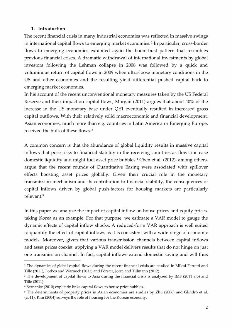
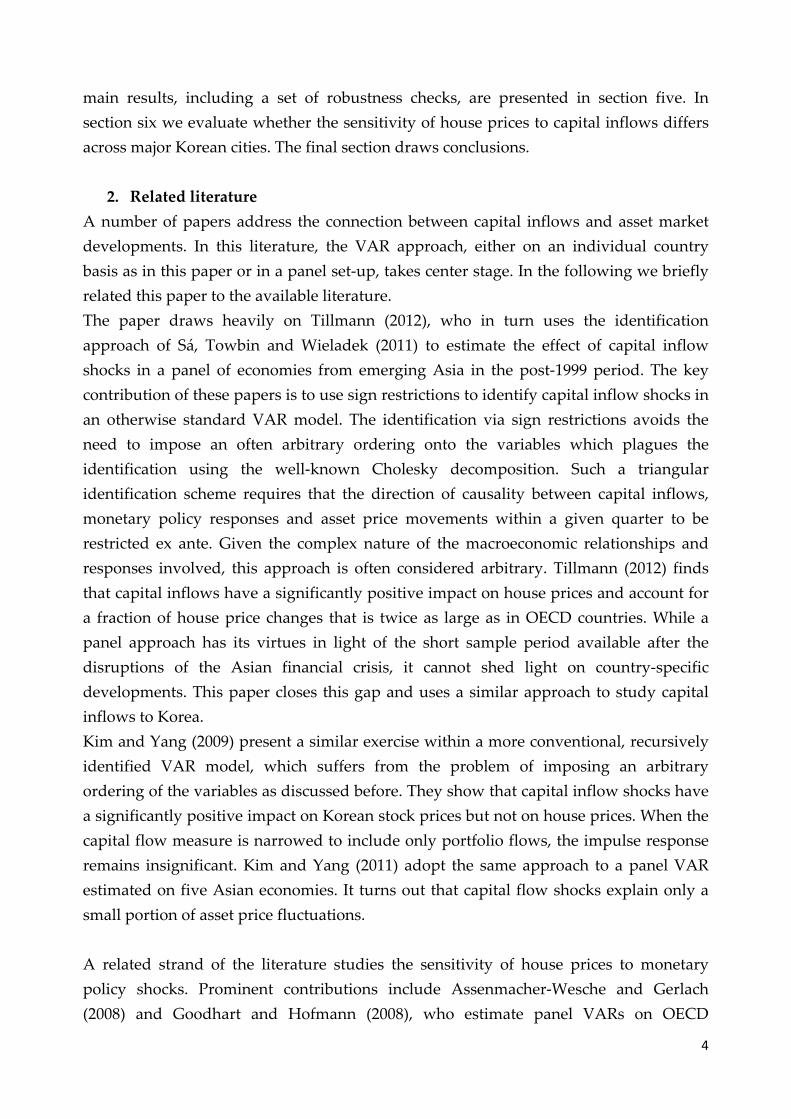
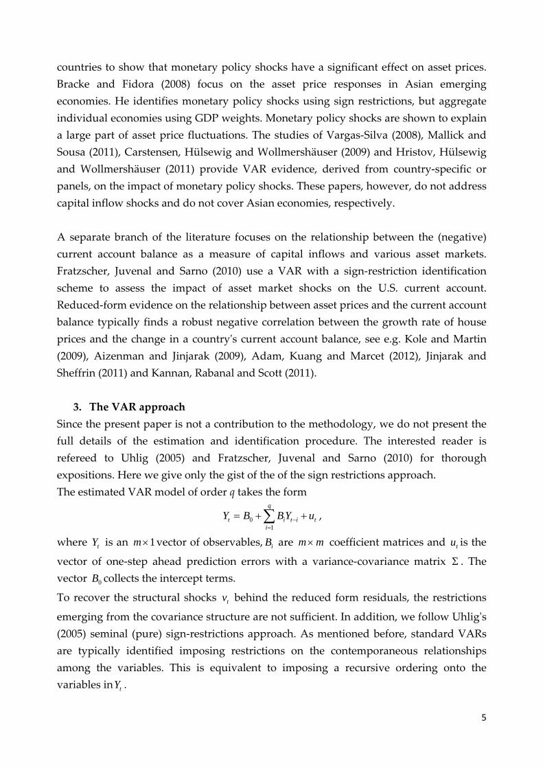
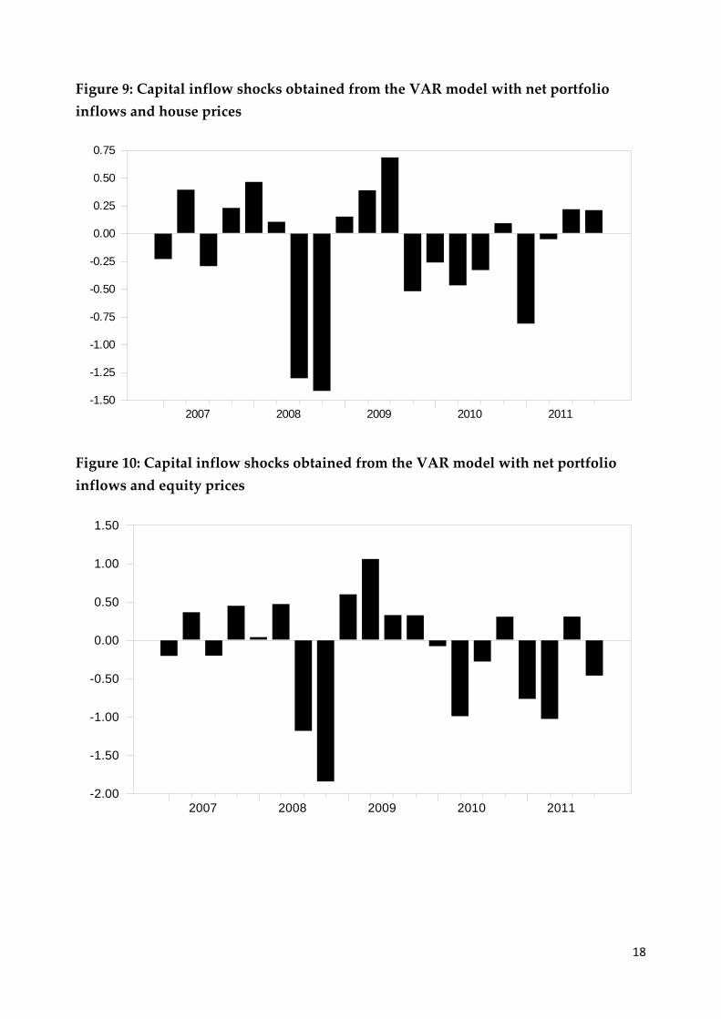
Shocks
Besides the impulse response functions and the corresponding forecast error variance
decomposition, the VAR models also deliver the series of identified capital inflow
shocks. These shocks are plotted in figures (7) to (12) for the alternative specifications.
The shock series from the baseline model, see figure (7), persuasively reflect the
evolution of the global financial crisis since 2008. The third and fourth quarter of 2008
are characterized by negative capital inflow shocks as global investors repatriated their
funds following the Lehman collapse. Triggered by the onset of a wave of
unconventional monetary policy measures in many mature economies since mid‐2009,
which lead to massive injections of liquidity, and a promise to keep interest rates low for
an extended period of time, large positive capital inflow shocks are observed. The quick
reversal in capital inflow shocks is even more pronounced when derived from the VAR
with portfolio inflows, see figures (9) and (10). In sum, the series of shocks complies
with the observable evolution of capital flows to Korea.
17
Figure 7: Capital inflow shocks obtained from the VAR model with net total inflows
and house prices
2007 2008 2009 2010 2011-1.25
-1.00
-0.75
-0.50
-0.25
0.00
0.25
0.50
0.75
Figure 8: Capital inflow shocks obtained from the VAR model with net total inflows
and equity prices
2007 2008 2009 2010 2011-1.50
-1.00
-0.50
0.00
0.50
1.00
18
Figure 9: Capital inflow shocks obtained from the VAR model with net portfolio
inflows and house prices
2007 2008 2009 2010 2011-1.50
-1.25
-1.00
-0.75
-0.50
-0.25
0.00
0.25
0.50
0.75
Figure 10: Capital inflow shocks obtained from the VAR model with net portfolio
inflows and equity prices
2007 2008 2009 2010 2011-2.00
-1.50
-1.00
-0.50
0.00
0.50
1.00
1.50
19
Figure 11: Capital inflow shocks obtained from the VAR model with gross total
inflows and house prices
2007 2008 2009 2010 2011-1.25
-1.00
-0.75
-0.50
-0.25
0.00
0.25
0.50
0.75
1.00
Figure 12: Capital inflow shocks obtained from the VAR model with gross total
inflows and equity prices
2007 2008 2009 2010 2011-1.00
-0.75
-0.50
-0.25
0.00
0.25
0.50
0.75
1.00
1.25
20
Robustness
To evaluate whether the previous set of findings is robust to changes in the estimation
sample and the choice of sign restrictions, we now present results from three
modifications. The first concerns the sample period. Since our baseline sample includes
the financial turbulence since 2008, we re‐estimate the VAR up to the second quarter of
2008, i.e. we truncate the sample before the Lehman collapse. The resulting impulse
responses are presented in figure (13). As a result, house prices again respond with an
increase of about one percent. Although this effect is more persistent than in the baseline
results, it is not statistically significant. The house price response might be suppressed
by a significant policy tightening, as reflected in the increase in the money market
interest rate, which is absent from the baseline model.
The second and third modification pertains to the set of sign restrictions. As discussed
before, we extent the restrictions proposed by Sá, Towbin and Wieladek (2011) by a
restriction on the output response. Since we include capital inflows as a ratio over GDP,
the joint restriction on capital inflows over GDP and GDP alone in fact imply a very
large increase in the level of capital inflows. Relaxing the constraint on output, see the
impulse responses in figure (14), leads to quantitatively unchanged results. The house
price response, although similarly shaped, is again on the border of significance.
Nevertheless, we believe the output response is necessary to model property price
booms and economic expansions fuelled by capital inflows.
In a third modification, we relax the restriction on the real exchange rate response. To
the extent capital inflows are absorbed by an accumulation of foreign exchange reserves
held by the Bank of Korea, the pressure on the real exchange rate can be contained. In
the case of Korea, the Monetary Stabilization Bonds issued by the Bank of Korea could
be used to sterilize the impact on domestic liquidity. Figure (15) presents the results for
a specification without an explicit REER restriction. While the house price response
remains significant, we see that the real exchange rate persistently appreciates even if
being unconstrained. Thus, the restriction on the real exchange rate used before is an
innocuous constrained.
21
Figure 13: Impulse responses to a capital inflow shock obtained from VAR model
with net total inflows and house prices estimated up to 2008:2
Impulse Responses for flows
0 1 2 3 4 5 6 7 8 9 10 11 12 13 14 15-2.00
0.00
2.00
4.00
Impulse Responses for GDP
0 1 2 3 4 5 6 7 8 9 10 11 12 13 14 15-2.00
-1.00
0.00
1.00
2.00
Impulse Responses for CPI
0 1 2 3 4 5 6 7 8 9 10 11 12 13 14 15-1.00
-0.50
0.00
0.50
1.00
Impulse Responses for house prices
0 1 2 3 4 5 6 7 8 9 10 11 12 13 14 15-2.00
-1.00
0.00
1.00
2.00
3.00
Impulse Responses for reer
0 1 2 3 4 5 6 7 8 9 10 11 12 13 14 15-10.00
-5.00
0.00
5.00
10.00
Impulse Responses for short rate
0 1 2 3 4 5 6 7 8 9 10 11 12 13 14 15-1.00
-0.50
0.00
0.50
Impulse Responses for long rate
0 1 2 3 4 5 6 7 8 9 10 11 12 13 14 15-1.00
-0.50
0.00
0.50
Notes: Each figure depicts the median response (solid line) and the 16th and 84th
percentiles of the accepted draws as a confidence band (dotted lines). The shaded areas
indicate the restrictions imposed.
22
Figure 14: Impulse responses to a capital inflow shock obtained from VAR model
with net total inflows and house prices, but without a sign restriction on GDP
Impulse Responses for flows
0 1 2 3 4 5 6 7 8 9 10 11 12 13 14 15-0.50
0.00
0.50
1.00
1.50
2.00
Impulse Responses for GDP
0 1 2 3 4 5 6 7 8 9 10 11 12 13 14 15-0.60
-0.30
0.00
0.30
0.60
Impulse Responses for CPI
0 1 2 3 4 5 6 7 8 9 10 11 12 13 14 15-0.50
-0.25
0.00
0.25
Impulse Responses for house prices
0 1 2 3 4 5 6 7 8 9 10 11 12 13 14 15-1.00
-0.50
0.00
0.50
1.00
1.50
Impulse Responses for reer
0 1 2 3 4 5 6 7 8 9 10 11 12 13 14 15-2.00
0.00
2.00
4.00
6.00
Impulse Responses for short rate
0 1 2 3 4 5 6 7 8 9 10 11 12 13 14 15-0.20
-0.10
0.00
0.10
0.20
0.30
Impulse Responses for long rate
0 1 2 3 4 5 6 7 8 9 10 11 12 13 14 15-0.40
-0.20
0.00
0.20
Notes: Each figure depicts the median response (solid line) and the 16th and 84th
percentiles of the accepted draws as a confidence band (dotted lines). The shaded areas
indicate the restrictions imposed.
23
Figure 15: Impulse responses to a capital inflow shock obtained from VAR model
with net total inflows and house prices, but without a sign restriction on REER
Impulse Responses for flows
0 1 2 3 4 5 6 7 8 9 10 11 12 13 14 15-0.50
0.00
0.50
1.00
1.50
2.00
Impulse Responses for GDP
0 1 2 3 4 5 6 7 8 9 10 11 12 13 14 15-0.25
0.00
0.25
0.50
0.75
Impulse Responses for CPI
0 1 2 3 4 5 6 7 8 9 10 11 12 13 14 15-0.40
-0.20
0.00
0.20
0.40
Impulse Responses for house prices
0 1 2 3 4 5 6 7 8 9 10 11 12 13 14 15-0.50
0.00
0.50
1.00
1.50
2.00
Impulse Responses for reer
0 1 2 3 4 5 6 7 8 9 10 11 12 13 14 15-2.00
0.00
2.00
4.00
Impulse Responses for short rate
0 1 2 3 4 5 6 7 8 9 10 11 12 13 14 15-0.20
-0.10
0.00
0.10
0.20
Impulse Responses for long rate
0 1 2 3 4 5 6 7 8 9 10 11 12 13 14 15-0.30
-0.20
-0.10
0.00
0.10
Notes: Each figure depicts the median response (solid line) and the 16th and 84th
percentiles of the accepted draws as a confidence band (dotted lines). The shaded areas
indicate the restrictions imposed.
6. Aggregate vs. regional effects
The analysis in the previous section showed the response of the aggregate Korean house
price index to a capital inflow shock. Given the uneven distribution of economic activity
across Korean metropolitan areas with a very high degree of centralization in Seoul, i.e.
the capital, it is interesting to gauge how representative this aggregate response patterns
is. 10 For that purpose we collect house price indexes for the seven largest Korean cities,
i.e. Seoul, Incheon, Busan, Daejon, Daeju, Gwangju and Ulsan.11 The three different VAR
models are estimated seven times, each time with the nationwide house price index
replaced by one of these seven regional house price series. All other variables remain
10 See Park, Bahng and Park (2010) for an analysis of regional differences in Korean property price
dynamics. 11 Regional house price data is taken from the CEIC database.
24
unchanged. This delivers seven sets of different impulse response functions, one for
each of the seven cities. Comparing these impulse responses reveals whether the
sensitivity of house prices to capital inflows differs across cities. A similar analysis is
conducted with respect to house prices within Seoul. We estimate two separate VARs
with house prices in the northern part and the southern part of Seoul. With its rapid
expansion, the southern part might be particularly prone to capital inflows from abroad.
Note that it is one advantage of the sign restrictions approach to shock identification
that changing the house price series is an innocuous modification as we do not have to
impose a certain contemporaneous interaction among the variables. Put differently, in a
standard recursive VAR replacing national house prices with prices in, say, Ulsan, is
likely to change the causality within the current quarter as prices in Ulsan might exhibit
a different relationship with aggregate macroeconomic variables than nation‐wide
house prices. Under the sign restrictions approach, however, we can easily substitute the
variable without affecting the identification scheme.
The resulting impulse response functions for the seven Korean cities are shown in
figures (16) to (18). In each figure we contrast the city‐specific median impulse response
with the confidence bands of the responses of aggregate house prices. Based on net total
capital inflows the house prices response in most cities lies within the confidence
bounds of the aggregate house price response. Put differently, the house price response
appears largely symmetric across cities. Only in Busan and Gwangju house prices
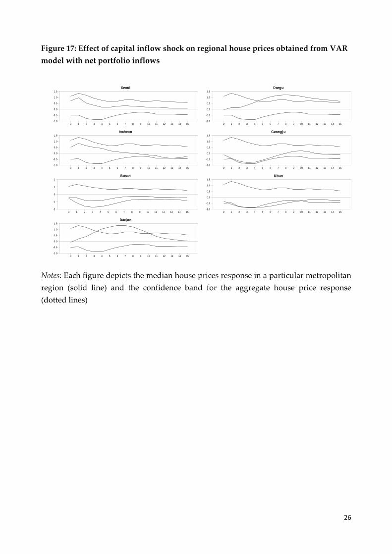
respond far less to capital inflows. Based on net portfolio flows, see figure (16), the
response in Busan and Ulsan is significantly below that of the nation‐wide house price
index, while house prices exhibit an above average appreciation in Daejon and Daegu.
The largest degree of regional heterogeneity obtains for the VAR model with gross
capital inflows, see figure (18). While house prices in Seoul and Incheon increase by
more than the nation‐wide average, prices in Gwangju and Busan increase by far less or
even fall after a capital inflow shock. The size of this regional discrepancy in terms of the
difference in maximum house prices responses is about two percentage points.
Figure (19) shows the impulse responses for a similar experiment, in which aggregate
house prices are replaced with house prices in either the northern part of Seoul, i.e. the
historical and administrative center, or the booming southern part of Seoul, which was
rapidly growing over the past decades and is home to many multinational companies.
Again the confidence bands are those from the aggregate house price response. While
the sensitivity of house prices to capital flows in the northern part of Seoul is fairly
representative for the entire country, the response in the southern part is significantly
stronger.
25
Figure 16: Effect of capital inflow shock on regional house prices obtained from VAR
model with net total inflows
Seoul
0 1 2 3 4 5 6 7 8 9 10 11 12 13 14 15-0.5
0.0
0.5
1.0
1.5
2.0
Incheon
0 1 2 3 4 5 6 7 8 9 10 11 12 13 14 15-0.5
0.0
0.5
1.0
1.5
2.0
Busan
0 1 2 3 4 5 6 7 8 9 10 11 12 13 14 15-1
0
1
2
Daejon
0 1 2 3 4 5 6 7 8 9 10 11 12 13 14 15-0.5
0.0
0.5
1.0
1.5
2.0
Daegu
0 1 2 3 4 5 6 7 8 9 10 11 12 13 14 15-0.5
0.0
0.5
1.0
1.5
2.0
Gwangju
0 1 2 3 4 5 6 7 8 9 10 11 12 13 14 15-0.5
0.0
0.5
1.0
1.5
2.0
Ulsan
0 1 2 3 4 5 6 7 8 9 10 11 12 13 14 15-0.5
0.0
0.5
1.0
1.5
2.0
Notes: Each figure depicts the median house prices response in a particular metropolitan
region (solid line) and the confidence band for the aggregate house price response
(dotted lines)
26
Figure 17: Effect of capital inflow shock on regional house prices obtained from VAR
model with net portfolio inflows
Seoul
0 1 2 3 4 5 6 7 8 9 10 11 12 13 14 15-1.0
-0.5
0.0
0.5
1.0
1.5
Incheon
0 1 2 3 4 5 6 7 8 9 10 11 12 13 14 15-1.0
-0.5
0.0
0.5
1.0
1.5
Busan
0 1 2 3 4 5 6 7 8 9 10 11 12 13 14 15-2
-1
0
1
2
Daejon
0 1 2 3 4 5 6 7 8 9 10 11 12 13 14 15-1.0
-0.5
0.0
0.5
1.0
1.5
Daegu
0 1 2 3 4 5 6 7 8 9 10 11 12 13 14 15-1.0
-0.5
0.0
0.5
1.0
1.5
Gwangju
0 1 2 3 4 5 6 7 8 9 10 11 12 13 14 15-1.0
-0.5
0.0
0.5
1.0
1.5
Ulsan
0 1 2 3 4 5 6 7 8 9 10 11 12 13 14 15-1.0
-0.5
0.0
0.5
1.0
1.5
Notes: Each figure depicts the median house prices response in a particular metropolitan
region (solid line) and the confidence band for the aggregate house price response
(dotted lines)
27
Figure 18: Effect of capital inflow shock on regional house prices obtained from VAR
model with gross total inflows
Seoul
0 1 2 3 4 5 6 7 8 9 10 11 12 13 14 15-1.0
-0.5
0.0
0.5
1.0
1.5
Incheon
0 1 2 3 4 5 6 7 8 9 10 11 12 13 14 15-1.0
-0.5
0.0
0.5
1.0
1.5
Busan
0 1 2 3 4 5 6 7 8 9 10 11 12 13 14 15-2
-1
0
1
2
Daej on
0 1 2 3 4 5 6 7 8 9 10 11 12 13 14 15-1.0
-0.5
0.0
0.5
1.0
1.5
Daegu
0 1 2 3 4 5 6 7 8 9 10 11 12 13 14 15-1.0
-0.5
0.0
0.5
1.0
1.5
Gwangj u
0 1 2 3 4 5 6 7 8 9 10 11 12 13 14 15-1.0
-0.5
0.0
0.5
1.0
1.5
Ulsan
0 1 2 3 4 5 6 7 8 9 10 11 12 13 14 15-1.0
-0.5
0.0
0.5
1.0
1.5
Notes: Each figure depicts the median house prices response in a particular metropolitan
region (solid line) and the confidence band for the aggregate house price response
(dotted lines)
28
Figure 19: Effect of capital inflow shock on house prices in different parts of Seoul
obtained from VAR model with net total inflows
Seoul: North
0 1 2 3 4 5 6 7 8 9 10 11 12 13 14 15-0.5
0.0
0.5
1.0
1.5
2.0
Seoul: South
0 1 2 3 4 5 6 7 8 9 10 11 12 13 14 15-0.5
0.0
0.5
1.0
1.5
2.0
Notes: Each figure depicts the median house prices response in a part of Seoul (solid
line) and the confidence band for the aggregate house price response (dotted lines)
The finding of sizable regional asymmetries in the responses to capital inflow shocks has
important implications for the design of policy directed towards avoiding overheating
property markets and house price bubbles, respectively. Our results tend to favor
macroprudential policy measures such as maximum debt‐to‐income ratios or maximum
loan‐to‐value‐ratios over standard monetary policy measures such as adjustment of the
short‐term interest rates to combat property price bubbles. While the former set of tool
can be tailored to the needs of regions housing market developments, the latter, i.e. a
monetary tightening, is too blunt a tool as it affect all regional property markets
symmetrically.
7. Conclusions
Large and volatile capital inflows into emerging economies, while generally considered
beneficial for growth and development, are often also associated with side effects such
as real exchange rate changes, effects on domestic liquidity and an increase in the
29
procyclicality of asset price movements. In this paper we took Korea as an example and
quantified the response of house and equity prices to a shock in capital inflows. The
VAR model estimated for that purpose revealed that suitably identified capital inflow
shocks indeed have a significantly positive impact on domestic house prices. Moreover,
this impact is unevenly spread across metropolitan areas.
These findings highlight the need to closely monitor asset price development in light of
massive capital inflows. Korea, among other countries in the region, pioneered the use
of macroprudential measures such as caps on loan‐to‐value ratios to contain the
property price boom. The results in this paper support this policy as, first, exogenous
capital flows stemming from foreign investors’ search for yield might lead to asset price
misalignments and, second, the impact is asymmetric across housing markets. The latter
property makes it difficult to combat asst price bubbles with an “aggregate tool” such as
a conventional monetary tightening. It should be taken into account, however, that
according to our results capital inflow shocks still account for only a small part of asset
price movements. Furthermore, the effectiveness of the initiatives taken by the Korean
authorities, e.g. the bank levy on non‐core liabilities that became effective in 2011 or the
adjustment of maximum loan‐to‐value rations, has to be carefully analyzed once
sufficient data is available.12
Finally, the sensitivity of asset markets to capital inflows implies risks for the Korean
housing market once capital flows are reversed e.g. due to a monetary tightening in
industrial countries.
12 See Igan and Kang (2011) for a first attempt.
30
References
Adam, K., P. Kuang and A. Marcet (2012): “House price booms and the current
account”, D. Acemoglu and M. Woodford (eds.), NBER Macroeconomics Annual
2011, 77‐122.
Aizenman, J. and Y. Jinjarak (2009): “Current account patterns and national real estate
markets”, Journal of Urban Economics 66, 75‐89.
Assenmacher‐Wesche, K. and S. Gerlach (2008): “Monetary policy, asset prices and
macroeconomic conditions: a panel‐VAR study”, unpublished, Goethe University
Frankfurt.
Bernanke, B. S. (2010): “Monetary policy and the housing bubble”, speech at the Annual
Meeting of the American Economic Association, Atlanta, January 3, 2010.
Bracke, T., and M. Fidora (2008): “Global liquidity glut or global savings glut? A
structural approach”, ECB Working Paper No. 911, European Central Bank.
Cardarelli, R., S. Elekdag and M. Ayhan Kose (2010): “Capital inflows: macroeconomic
implications and policy responses”, Economic Systems 34, 333‐356.
Carstensen, K., O. Hülsewig and T. Wollmershäuser (2009): “Monetary policy
transmission and house prices: European cross‐country evidence”, CESifo
Working Paper No. 2750, ifo Institute for Economic Research at the University of
Munich.
Chen, Q., A. Filardo, D. He and F. Zhu (2012): “International spillovers of central bank
balance sheet policies”, BIS Papers No. 66, 220‐264, Bank for International
Settlements.
Chung, K. (2010): “Mechanisms to mitigate the adverse effect of capital inflows: Korea’s
experience”, unpublished, Bank of Korea.
Crowe, C., G. Dell’Ariccia, D. Igan and P. Rabanal (2011): “Policies for macrofinancial
stability: options to deal with real estate booms”, IMF Staff Discussion Note
SDN/11/02, International Monetary Fund.
Förster, M., M. Jorra and P. Tillmann (2012): “The dynamics of international capital
flows: results from a dynamic hierarchical factor model”, MAGKS Working Paper
No. 21‐2012, University of Giessen.
Forbes, K. J. and F. E. Warnock (2011): “Capital flow waves: surges, stops, flights and
retrenchment”, NBER Working Paper No. 17351, National Bureau of Economic
Research.
Fratzscher, M., L. Juvenal and L. Sarno (2010): “Asset prices, exchange rates and the
current account”, European Economic Review 54, 643‐658.
Fratzscher, M., M. Lo Duca and R. Straub (2012): “Quantitative Easing, portfolio choice
and international capital flows”, unpublished, European Central Bank.
31
Glindro, E. T., T. Subhanij, J. Szeto and H. Zhu (2011): “Determinants of house prices in
nine Asia‐Pacific economies”, International Journal of Central Banking 7, 163‐204.
Goodhart, C. and B. Hofmann (2008): “House prices, money, credit, and the
macroeconomy”, Oxford Review of Economic Policy 24, 180‐205.
Hristov, N., O. Hülsewig and T. Wollmershäuser (2011): “Loan supply shocks during
the financial crisis: evidence for the euro area from a panel VAR with sign
restrictions”, forthcoming, Journal of International Money and Finance.
Igan, D. and H. Kang (2011): “Do loan‐to‐value and debt‐to‐income limits work?
Evidence from Korea”, IMF Working Paper WP/11/297, International
Monetary Fund.
IMF (2011a): “International capital flows: reliable of fickle?”, IMF World Economic
Outlook, chapter 4, April 2011, International Monetary Fund.
IMF (2011b): “Capital flows to Asia: comparison with previous experience and monetary
policy options”, IMF Regional Economic Outlook Asia and Pacific, chapter 2, April
2011, International Monetary Fund.
Jinjarak, Y. and S. M. Sheffrin (2011): “Causality, real estate prices, and the current
account”, Journal of Macroeconomics 33, 233‐246.
Jongwanich, J. (2010): “Capital flows and real exchange rates in emerging Asian
countries”, ADB Economics Working Paper Series No. 210, Asian Development
Bank.
Kannan, R., P. Rabanal and A. Scott (2011): “Recurring patterns in the run‐up to house