Capital is Back:

Wealth-Income Ratios in Rich Countries 1700-2010

Thomas PikettyParis School of Economics

Gabriel ZucmanParis School of Economics

July 26, 2013⇤

Abstract

How do aggregate wealth-to-income ratios evolve in the long run and why? We addressthis question using 1970-2010 national balance sheets recently compiled in the top eightdeveloped economies. For the U.S., U.K., Germany, and France, we are able to extend ouranalysis as far back as 1700. We find in every country a gradual rise of wealth-income ratiosin recent decades, from about 200-300% in 1970 to 400-600% in 2010. In e↵ect, today’sratios appear to be returning to the high values observed in Europe in the eighteenth andnineteenth centuries (600-700%). This can be explained by a long run asset price recovery(itself driven by changes in capital policies since the world wars) and by the slowdownof productivity and population growth, in line with the � = s/g Harrod-Domar-Solowformula. That is, for a given net saving rate s = 10%, the long run wealth-income ratio �is about 300% if g = 3% and 600% if g = 1.5%. Our results have important implicationsfor capital taxation and regulation and shed new light on the changing nature of wealth,the shape of the production function, and the rise of capital shares.

⇤Thomas Piketty: piketty@pse.ens.fr; Gabriel Zucman: zucman@pse.ens.fr. We are grateful to seminar par-ticipants at the Paris School of Economics, Sciences Po, the International Monetary Fund, Columbia University,University of Pennsylvania, the European Commission, the University of Copenhagen, and the NBER summerinstitute for their comments and reactions. A detailed Data Appendix supplementing the present working pa-per is available online: http://piketty.pse.ens.fr/capitalisback and http://www.gabriel-zucman.eu/capitalisback.

1 Introduction

This paper addresses what is arguably one the most basic economic questions: how do wealth-

income and capital-output ratios evolve in the long run, and why?

Until recently it was di�cult to properly address this question, for one simple reason: na-

tional accounts were mostly about flows, not stocks. Economists had at their disposal a large

body of historical series on flows of output, income and consumption – but limited data on stocks

of assets and liabilities. When needed, for example for growth accounting exercises, estimates of

capital stocks were typically obtained by cumulating past flows of saving and investment. This

is fine for some purposes, but severely limits the set of questions one can ask.

In recent years, the statistical institutes of nearly all developed countries have started pub-

lishing retrospective national stock accounts including annual and consistent balance sheets.

Following new international guidelines, the balance sheets report on the market value of all the

non-financial and financial assets and liabilities held by each sector of the economy (households,

government, and corporations) and by the rest of the world. They can be used to measure the

stocks of private and national wealth at current market value.

This paper makes use of these new balance sheets in order to establish a number of facts

and to analyze whether standard capital accumulation models can account for these facts. We

should stress at the outset that we are well aware of the deficiencies of existing balance sheets.

In many ways these series are still in their infancy. But they are the best data that we have

in order to study wealth accumulation – a question that is so important that we cannot wait

for perfect data before we start addressing it, and that has indeed been addressed in the past

by many authors using far less data than we presently have. In addition, we feel that the best

way for scholars to contribute to future data improvement is to use existing balance sheets in a

conceptually coherent manner, so as to better identify their limitations. Our paper, therefore,

can also be viewed as an attempt to evaluate the internal consistency of the flow and stock sides

of existing national accounts, and to pinpoint the areas in which progress needs to be made.

Our contribution is twofold. First, we put together a new macro-historical data set on wealth

and income, available online, whose main characteristics are summarized in Table 1. To our

knowledge, it is the first international database to include long-run, homogeneous information

on national wealth. For the eight largest developed economies in the world – the U.S., Japan,

Germany, France, the U.K., Italy, Canada, and Australia – we have o�cial annual series covering

1

the 1970-2010 period. Through to the world wars, there was a lively tradition of national wealth

accounting in many countries. By combining numerous historical estimates in a systematic and

consistent manner, we are able to extend our series as far back as 1870 (Germany), 1770 (U.S.),

and 1700 (U.K. and France). The resulting database provides extensive information on the

structure of wealth, saving, and investment. It can be used to study core macroeconomic

questions – such as private capital accumulation, the dynamics of the public debt, and patterns

in net foreign asset positions – altogether and over unusually long periods of time.

Our second – and most important – contribution is to exploit the database in order to

establish a number of new striking results. Looking first at the recent period, we document that

wealth-income ratios have been gradually rising in each of the top eight developed countries over

the last four decades, from about 200-300% in 1970 to 400-600% in 2010 (Figure 1). Taking

a long-run perspective, we find that today’s ratios appear to be returning to the high values

observed in Europe in the eighteenth and nineteenth centuries, namely about 600-700%, despite

considerable changes in the nature of wealth (Figure 2 and 3). In the U.S., the wealth-income

ratio has also followed a U-shaped pattern, but less marked (Figure 4).

In order to understand these dynamics, we provide detailed decompositions of wealth accu-

mulation into volume e↵ects (saving) and relative price e↵ects (real capital gains and losses).

The results show that the U-shaped evolution of the European wealth-income ratios can be ex-

plained by two main factors. The first is a long-run swing in relative asset prices, itself largely

driven by changes in capital policies in the course of the twentieth century. Before World War

I, capital markets ran unfettered. A number of anti-capital policies were then put into place,

which depressed asset prices through to the 1970s. These policies were gradually lifted from the

1980s on, contributing to an asset price recovery.

The second key explanation for the return of high wealth-income ratios is the slowdown of

productivity and population growth. According to the Harrod-Domar-Solow formula, in the

long run the wealth-income ratio � is equal to the net saving rate s divided by the income

growth rate g. So for a given saving rate s =10%, the long-run � is about 300% if g = 3% and

about 600% if g = 1.5%. In short: capital is back because low growth is back.

The � = s/g formula is simple, yet as we show in the paper surprisingly powerful. It can

account for a significant part of the 1970-2010 rise in the wealth-income ratios of Europe and

Japan, two economies where population and productivity growth have slowed markedly. It

2

can also explain why wealth-income ratios are lower in the U.S., where population growth has

been historically much larger than in Europe – and still continues to be to some extent – but

where saving rates are not higher. Last, the Harrod-Domar-Solow formula seems to account

reasonably well for the very long-run dynamics of wealth accumulation. Over a few years and

even a few decades, valuation e↵ects and war destructions are of paramount importance. But in

the main developed economies, we find that today’s wealth levels are reasonably well explained

by 1870-2010 saving and income growth rates, in line with the workhorse one-good model of

capital accumulation. In the long run, assuming a significant divergence between the price of

consumption and capital goods seems unnecessary.

Our findings have a number of implications for the future and for policy-making. First, the

low wealth-income ratios of the mid-twentieth century were due to very special circumstances.

The world wars and anti-capital policies destroyed a large fraction of the world capital stock

and reduced the market value of private wealth, which is unlikely to happen again with free

markets. By contrast, the � = s/g logic will in all likelihood matter a great deal in the

foreseeable future. As long as they keep saving sizable amounts (due to a mixture of bequest,

life-cycle and precautionary reasons), countries with low g are bound to have high �. For the

time being, this e↵ect is strong in Europe and Japan. To the extent that growth will ultimately

slow everywhere, wealth-income ratios may well ultimately rise in the whole world.

The return of high wealth-income ratios is certainly not bad in itself, but it raises new issues

about capital taxation and regulation. Because wealth is always very concentrated (due in

particular to the cumulative and multiplicative processes governing wealth inequality dynamics),

high � implies than the inequality of wealth, and potentially the inequality of inherited wealth, is

likely to play a bigger role for the overall structure of inequality in the twenty first century than

it did in the postwar period. This evolution might reinforce the need for progressive capital and

inheritance taxation (Piketty, 2011; Piketty and Saez, 2013). If international tax competition

prevents this policy change from happening, one cannot exclude the development of a new wave

of anti-globalization and anti-capital policies.

Further, because s and g are largely determined by di↵erent forces, wealth-income ratios

can vary a lot between countries. This fact has important implications for financial regulation.

With perfect capital markets, large di↵erences in wealth-income ratios potentially imply large

net foreign asset positions, which can create political tensions between countries. With imperfect

3

capital markets and home portfolios bias, structurally high wealth-income ratios can contribute

to domestic asset price bubbles. According to our computations, the wealth-income ratio reached

700% at the peak of the Japanese bubble of the late 1980s, and 800% in Spain in 2008-2009.1

Housing and financial bubbles are potentially more devastating when the total stock of wealth

amounts to 6-8 years of national income rather than 2-3 years only. The fact that the Japanese

and Spanish bubbles are easily identifiable in our dataset also suggests that monitoring wealth-

income ratios may help designing appropriate financial and monetary policy. In Japan and

Spain, most observers had noticed that asset price indexes were rising fast. But in the absence

of well-defined reference points, it is always di�cult for policy makers to determine when such

evolutions have gone too far and whether they should act. We believe that wealth-income ratios

and wealth accumulation decompositions provide useful if imperfect reference points.

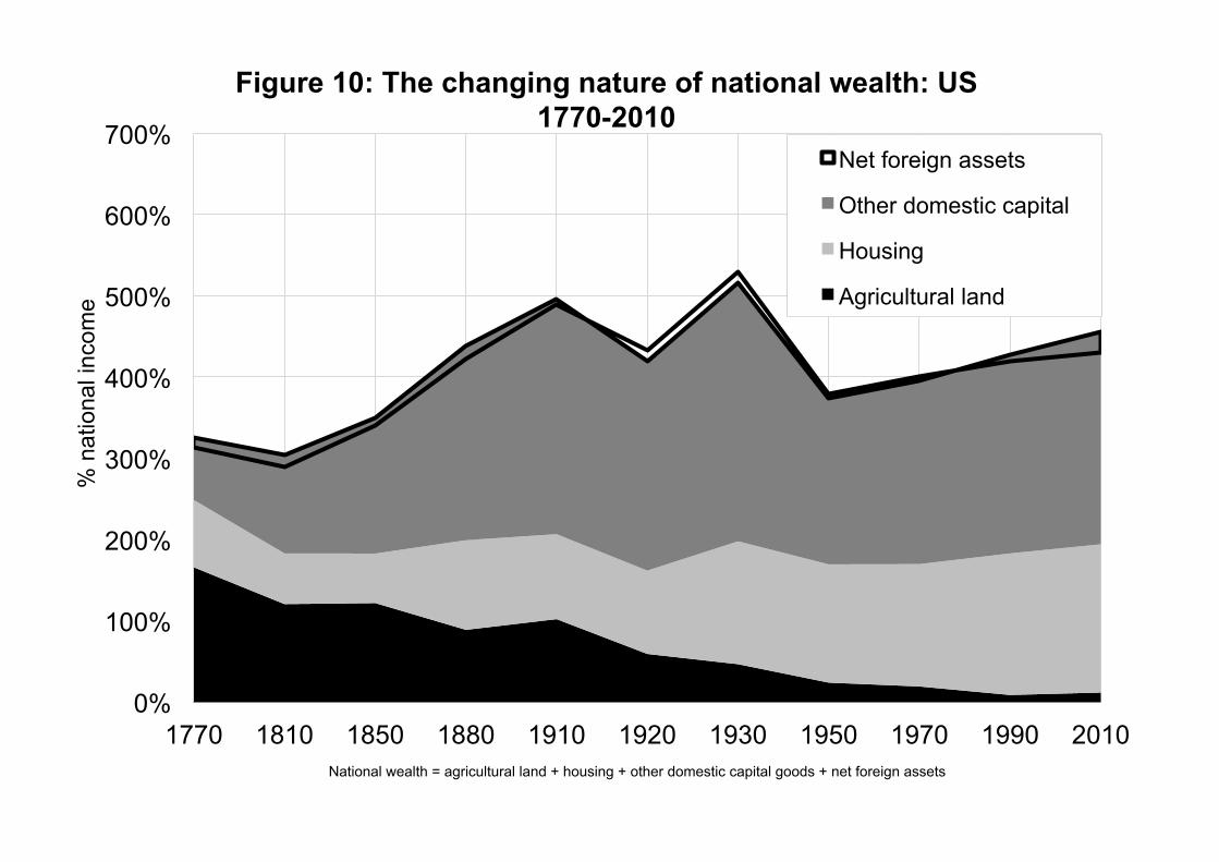
Last, our findings shed new light on the long run changes in the nature of wealth, the shape of

the production function and the recent rise in capital shares. In the 18th and early 19th century,

capital was mostly land (Figure 3), so that there was limited scope for substituting labor to

capital. In the 20th and 21st centuries, by contrast, capital takes many forms, to an extent such

that the elasticity of substitution between labor and capital might well be larger than 1. With

an elasticity even moderately larger than 1, rising capital-output ratios can generate substantial

increases in capital shares, similar to those that have occurred in most rich countries since the

1970s. Looking forward, with low growth and high wealth-income ratios, one cannot exclude a

further increase in capital shares.

The paper is organized as follows. Section 2 relates our work to the existing literature. In

section 3 we present the conceptual framework and accounting equations used in this research.

Section 4 is devoted to the decomposition of wealth accumulation in rich countries over the 1970-

2010 period. In section 5, we present decomposition results over a longer period (1870-2010)

for a subset of countries (U.S., Germany, France, U.K.). We take an even longer perspective

in section 6 in which we discuss the changing nature of wealth in the U.K., France and the

U.S. since the 18th century. In section 7, we compare the long-run evolution of capital-output

ratios and capital shares in order to discuss the changing nature of technology and the pros

and cons of the Cobb-Douglas approximation. Section 8 presents some possible directions for

1See Appendix figure A8. We do not include Spain in our main sample of countries because the Bank ofSpain balance sheets that are currently available only start in 1987, and we want to be able to decompose wealthaccumulation over a longer period (at least 1970-2010).

4

future research. The main sources and concepts are presented in the main text, and we leave

the complete methodological details to an extensive online Data Appendix.

2 Related literature

2.1 Literature on national wealth

As far as we know, this paper is the first attempt to gather a large set of national balance sheets

in order to analyze the long-run evolution of wealth-income ratios. For a long time, research in

this area was impeded by a lack of data. It is only in 1993 that the System of National Accounts,

the international standard for national accounting, first included guidelines for wealth. In most

rich countries, the publication of time series of national wealth only began in the 1990s and

2000s. In a key country like Germany, the first o�cial balance sheets were released in 2010.

It is worth stressing, however, that the recent emphasis on national wealth largely represents

a return to older practice. Until the early twentieth century, economists, statisticians and social

arithmeticians were much more interested in computing national wealth than national income

and output. The first national balance sheets were established in the late seventeenth and early

eighteenth centuries by Petty (1664) and King (1696) in the U.K., Boisguillebert (1695) and

Vauban (1707) in France. National wealth estimates then became plentiful in the nineteenth

and early twentieth century, with the work of Colqhoun (1815), Gi↵en (1889) and Bowley (1920)

in the U.K., Foville (1893) and Colson (1903) in France, Hel↵erich (1913) in Germany, King

(1915) in the U.S., and dozens of other economists from all industrialized nations. Although

these historical balance sheets are far from perfect, their methods are well documented and they

are usually internally consistent. One should also keep in mind that it was in many ways easier

to estimate national wealth around 1900-1910 than it is today: the structure of property was

much simpler, with far less financial intermediation and cross-border positions.

Following the 1914-1945 capital shocks, the long tradition of research on national wealth

largely disappeared, partly because of the new emphasis on short run output fluctuations fol-

lowing the Great Depression, and partly because the chaotic asset price movements of the

interwar made the computation of the current market value of wealth and the comparison with

pre-World War I estimates much more di�cult. While there has been some e↵ort to put to-

gether historical balance sheets in recent decades, most notably by Goldsmith (1985, 1991), to

date no systematic attempt has been made to relate the evolution of wealth-income ratios to the

5

magnitude of saving flows.2 The reason is probably that it is only recently that o�cial balance

sheets have become su�ciently widespread to make the exercise meaningful.

2.2 Literature on capital accumulation and growth

The lack of data on wealth in the aftermath of the 1914-1945 shocks did not prevent economists

from studying capital accumulation. In particular, Solow developed the neoclassical growth

model in the 1950s. In this model, the long-run capital-output ratio is equal to the ratio between

the saving rate and the growth rate of the economy. As is well-known, the � = s/g formula was

first derived by Harrod (1939) and Domar (1947) using fixed-coe�cient production functions, in

which case � is entirely given by technology – hence the knife-edge conclusions about growth.3

The classic derivation of the formula with a flexible production function Y = F (K,L) involving

capital-labor substitution, thereby making � endogenous and balanced growth possible, is due

to Solow (1956). Authors of the time had limited national accounts at their disposal to estimate

the parameters of the formula. In numerical illustrations, they typically took � = 400%, g = 2%,

and s = 8%. They were not entirely clear about the measurement of capital, however.

Starting in the 1960s, the Solow model was largely applied for empirical studies of growth

(see for instance Denison, 1962; Jorgenson and Griliches, 1967; Feinstein, 1978) and it was

later on extended to human capital (Mankiw, Romer and Weil, 1992; Barro, 1991). The main

di↵erence between our work and the growth accounting literature is how we measure capital.

Because of the lack of balance sheet data, in the growth literature capital is typically computed

by cumulating past investment flows and attempting to adjust for changes in price – what is

known as the perpetual inventory method. By contrast, we measure capital by using national

balance sheets in which we observe the actual evolution of the market value of most types of

assets: real estate, equities (which capture the market value of corporations), bonds, and so

on. We are essentially interested in what non-human private capital is worth for households

2In particular, Goldsmith does not relate his wealth estimates to saving and investment flows. He is mostlyinterested in the rise of financial intermediation, that is the rise of gross financial assets and liabilities (expressedas a fraction of national income), rather than in the evolution of the net wealth-income ratio. Nineteenth centuryauthors like Gi↵en and Foville were fascinated by the huge accumulation of private capital, but did not havemuch estimates of income, saving and investment, so they were not able to properly analyze the evolution of thewealth-income ratio. Surprisingly enough, socialist authors like Karl Marx – who were obviously much interestedin the rise of capital and the possibility that � reaches very high levels – largely ignored the literature on nationalwealth.

3Harrod emphasized the inherent instability of the growth process, while Domar stressed the possibility that� and s can adjust in case the natural growth rate g di↵ers from s/�.

6

at each point in time – and in what public capital would be worth if it was privatized. This

notion is precisely what the economists of the eighteenth and nineteenth century aimed to

capture. We believe it is a useful, meaningful, and well defined starting point.4 There are

two additional advantages to using balance sheets: first, they include data for a large number

of assets, including non-produced assets such as land which by definition cannot be measured

by cumulating past investment flows. Second, they rely for the most part on observed market

prices – such as actual real estate transactions and financial market quotes – contrary to the

prices used in the perpetual inventory method, which tend not to be well defined.5

Now that national balance sheets are available, we can see that some of the celebrated

stylized facts on capital – established when there was actually little data on capital – are not

that robust. The constancy of the capital-output ratio, in particular, is simply not a fact for

Europe and Japan, and is quite debatable for the U.S. Although this constancy is often seen as

one of the key regularities in economics, there has always been a lot of confusion about what

the level of the capital-output ratio is supposed to be (see, e.g., Kaldor, 1961; Samuelson, 1970;

Simon, 1990; Jones and Romer, 2010). The data we presently have suggest that the ratio is

often closer to 5-6 in most rich countries today than to the values of 3-4 typically used in macro

models and textbooks.6

Our results also suggest that the focus on the possibility of a balanced growth path that

has long characterized academic debates on capital accumulation (most notably during the

Cambridge controversy of the 1960s-1970s) has been somewhat misplaced. It is fairly obvious

that there can be a lot of capital-labor substitution in the long-run, and that many di↵erent �

can occur in steady-state. But this does not imply that the economy is necessarily in a stable

or optimal state in any meaningful way. High steady-state wealth-income ratios can go together

4By contrast, in the famous Cambridge controversy, the proponent of the U.K. view argued that the notionof capital used in neoclassical growth models is not well defined. In our view much of the controversy owes tothe lack of balance sheet data, and to the di�culty of making comparisons with pre-World War 1 estimates ofnational capital stocks.

5As we discuss in details in Appendix A.1.2, the price estimates used in the perpetual inventory method raiseall sorts of di�culties (depreciation, quality improvement, aggregation bias, etc.). Even when these di�cultiescan be overcome, PIM estimates of the capital stock at current price need not be equal to the current marketvalue of wealth. For instance, the current value of dwellings obtained by the PIM is essentially equal to pastinvestments in dwellings adjusted for the evolution of the relative price of construction. This has no reason tobe equal to the current market value of residential real estate – which in practice is often higher.

6Many estimates in the literature only look at the capital-output ratio in the corporate sector (i.e., corporatecapital divided by corporate product), in which case ratios of 3 or even 2 are indeed in line with the data(see Figures A70-A71). This, however, completely disregards the large stock of housing capital, as well asnon-corporate businesses and government capital.

7

with large instability, asset price bubbles and high degrees of inequality – all plausible scenarios

in mature, low-growth economies.

2.3 Literature on external balance sheets

Our work is close in spirit to the recent literature that documents and attempts to understand the

dynamics of the external balance sheets of countries (Lane and Milesi-Ferretti, 2007; Gourinchas

and Rey, 2007; Zucman, 2013). To some extent, what we are doing in this paper is to extend this

line of work to domestic wealth and to longer time periods. We document the changing nature

of domestic capital over time, and we investigate the extent to which the observed aggregate

dynamics can be accounted for by saving flows and valuation e↵ects. A key di↵erence is that our

investigation is broader in scope: as we shall see, domestic capital typically accounts for 90%-

110% of the total wealth of rich countries today, while the net foreign asset position accounts

for -10% to +10% only. Nevertheless, external wealth will turn out to play an important role in

the dynamics of the national wealth of a number of countries, more spectacularly the U.S. The

reason is that gross foreign positions are much bigger than net positions, thereby potentially

generating large capital gains or losses at the country level.7 One of the things we attempt to

do is to put the study of external wealth into the broader perspective of national wealth.8

2.4 Literature on rising capital shares

Our work is also closely related to the growing literature establishing that capital shares have

been rising in most countries over the last decades (Ellis and Smith, 2007; Azmat, Manning

and Van Reenen, 2011; Karabarbounis and Neiman, 2013). The fact that we find rising wealth-

income and capital-output ratios in the leading rich economies reinforces the presumption that

capital shares are indeed rising globally. We believe that this confirmation is important in itself,

because computing factor shares raises all sorts of issues. In many situations, what accrues to

labor and to capital is unclear – both in the non-corporate sector and in the corporate sector,

where profits and dividends recorded in the national accounts sometimes include labor income

components that are impossible to isolate. Wealth-income and capital-output ratios provide an

7See Obstfeld (2013) and Gourinchas and Rey (2013) for recent papers surveying the literature on this issue.8Eisner (1980), Babeau (1983), Greenwood and Wol↵ (1992), Wol↵ (1999), and Gale and Sabelhaus (1999)

study the dynamics of U.S. aggregate household wealth using o�cial balance sheets and survey data. With apure household perspective, however, one is bound to attribute an excessively large role to capital gains, becausea lot of private saving takes the form corporate retained earnings.

8

indication of the relative importance of capital in production largely immune to these issues,

although they are themselves not perfect. They usefully complement measures of factor shares.

More generally, we attempt to make progress in the measurement of three fundamentally

inter-related macroeconomic variables: the capital share, the capital-output ratio, and the

marginal product of capital (see also Caselli and Feyrer, 2007). As we discuss in section 7,

rising capital-output ratios together with rising capital shares and declining returns to capital

imply an elasticity of substitution between labor and capital higher than 1 – consistent with

the results obtained by Karabarbounis and Neiman (2013) over the same period of time.

2.5 Literature on income and wealth inequalities

Last, this paper is to a large extent the continuation of the study of the long run evolution of

private wealth in France undertaken by one of us (Piketty, 2011). We extend Piketty’s analysis

to many countries, to longer time periods, and to public and foreign wealth. However, we do

not decompose aggregate wealth accumulation into an inherited and dynastic wealth component

on the one hand and a lifecycle and self-made wealth component on the other (as Piketty does

for France). Instead, we take the structure of saving motives and the overall level of saving

as given. In future research, it would be interesting to extend our decompositions in order to

study the evolution of the relative importance of inherited versus life-cycle wealth in as many

countries as possible.

Ultimately, the goal is also to introduce global distributional trends in the analysis. Any

study of wealth inequality requires reliable estimates of aggregate wealth to start with. Plugging

distributions into our data set would make it possible to analyze the dynamics of the global

distribution of wealth.9 The resulting series could then be used to improve the top income shares

estimates that were recently constructed for a number of countries (see Atkinson, Piketty, Saez

2011). We see the present research as an important step in this direction.

3 Conceptual framework and methodology

3.1 Concepts and definitions

The concepts we use are standard: we strictly follow the U.N. System of National Accounts

(SNA). For the 1970-2010 period, we use o�cial national accounts that comply with the latest

9See Davies et al. (2010) for a study of the world distribution of wealth using national balance sheet data.

9

international guidelines (SNA, 1993, 2008). For the previous periods, we have collected a large

number of historical balance sheets and income series, which we have homogenized using the

same concepts and definitions as those used in the most recent o�cial accounts.10 Here we

provide the main definitions.

Private wealth Wt is the net wealth (assets minus liabilities) of households and non-profit

institutions serving households.11 Following SNA guidelines, assets include all the non-financial

assets – land, buildings, machines, etc. – and financial assets – including life insurance and

pensions funds – over which ownership rights can be enforced and that provide economic ben-

efits to their owners. Pay-as-you-go social security pension wealth is excluded, just like all

other claims on future government expenditures and transfers (like education expenses for one’s

children and health benefits). Durable goods owned by households, such as cars and furniture,

are excluded as well.12 As a general rule, all assets and liabilities are valued at their prevailing

market prices. Corporations are included in private wealth through the market value of equities.

Unquoted shares are typically valued on the basis of observed market prices for comparable,

publicly traded companies.

We similarly define public (or government) wealth Wgt as the net wealth of public adminis-

trations and government agencies. In available balance sheets, public non-financial assets like

administrative buildings, schools and hospitals are valued by cumulating past investment flows

and upgrading them using observed real estate prices.

We define market-value national wealth Wnt as the sum of private and public wealth:

Wnt = Wt +Wgt

National wealth can also be decomposed into domestic capital and net foreign assets:

Wnt = Kt +NFAt

10Section A of the Data Appendix provides a detailed description of the concepts and definitions used by the1993 and 2008 SNA. Country-specific information on historical balance sheets are provided in Data Appendixsections B (devoted to the U.S.), D (Germany), E (France), and F (U.K.).

11The main reason for including non-profit institutions serving households (NPISH) in private wealth is thatthe frontier between individuals and private foundations is not always entirely clear. The net wealth of NPISHis usually small, and always less than 10% of total net private wealth: currently it is about 1% in France, 3%-4%in Japan, and 6%-7% in the U.S., see Appendix Table A65. Note also that the household sector includes allunincorporated businesses.

12The value of durable goods appears to be relatively stable over time (about 30%-50% of national income,i.e. 5%-10% of net private wealth). See for instance Appendix Table US.6f for the long-run evolution of durablegoods in the U.S.

10

And domestic capital Kt can in turn be decomposed as the sum of agricultural land, housing,

and other domestic capital (including the market value of corporations, and the value of other

non-financial assets held by the private and public sectors, net of their liabilities).

An alternative measure of the wealth of corporations is the total value of corporate assets

net of non-equity liabilities, what we call the corporations’ book value. We define residual

corporate wealth Wct as the di↵erence between the book-value of corporations and their market

value (which is the value of their equities). By definition, Wct is equal to 0 when Tobin’s Q –

the ratio between market and book values – is equal to 1. In practice there are several reasons

why Tobin’s Q can be di↵erent from 1, so that residual corporate wealth is at times positive, at

times negative. We define book-value national wealth Wbt as the sum of market-value national

wealth and residual corporate wealth: Wbt = Wnt +Wct = Wt +Wgt +Wct. Although we prefer

our market-value concept of national wealth (or national capital), both definitions have some

merit, as we shall see.13

Balance sheets are constructed by national statistical institutes and central banks using

a large number of census-like sources, in particular reports from financial and non-financial

corporations about their balance sheet and o↵-balance sheet positions, and housing surveys.

The perpetual inventory method usually plays a secondary role. The interested reader is referred

to the Appendix for a a precise discussion of the methods used by the leading rich countries.

Regarding income, the definitions and notations are standard. Note that we always use

net-of-depreciation income and output concepts. National income Yt is the sum of net domestic

output and net foreign income: Yt = Ydt+rt·NFAt.14 Domestic output can be thought as coming

from some production function that uses domestic capital and labor as inputs: Ydt = F (Kt, Lt).

We are particularly interested in the evolution of the private wealth-national income ratio

�t = Wt/Yt and of the (market-value) national wealth-national income ratio �nt = Wnt/Yt. In

a closed economy – and more generally in an open economy with a zero net foreign position

– the national wealth-national income ratio �nt is the same as the domestic capital-output

13Wbt corresponds to the concept of “national net worth” in the SNA (see Data Appendix A.4.2). In thispaper, we propose to use “national wealth” and “national capital” interchangeably (and similarly for “domesticwealth” and “domestic capital”, and “private wealth” and “private capital”), and to specify whether one uses“market-value” or “book-value” aggregates. Note that 19th century authors such as Gi↵en and Foville also used“national wealth” and “national capital” interchangeably. The di↵erence is that they viewed market values asthe only possible value, while we recognize that both definitions have some merit (see below the discussion onGermany).

14National income also includes net foreign labor income and net foreign production taxes – both of which areusually negligible.

11

ratio �kt = Kt/Ydt.15 In case public wealth is equal to zero, then both ratios are also equal

to the private wealth-national income ratio: �t = �nt = �kt. At the global level, the world

wealth-income ratio is always equal to the world capital/output ratio.

We are also interested in the evolution of the capital share ↵t = rt ·�t. With imperfect capital

markets, the average rate of return rt can substantially vary across assets. In particular, it can

be di↵erent for domestic and foreign assets. With perfect capital markets, the rate of return

rt is the same for all assets and is equal to the marginal product of capital. With a Cobb-

Douglas production function F (K,L) = K↵L1�↵, and a closed economy setting, the capital

share is entirely set by technology: ↵t = rt · �t = ↵. A higher capital-output ratio �t is exactly

compensated by a lower capital return rt = ↵/�t, so that the product of the two is constant.

In an open economy setting, the world capital share is also constant and equal to ↵, and the

world rate of return is also given by rt = ↵/�t, but the countries with higher-than-average

wealth-income ratios invest part of their wealth in other countries, so that for them the share

of capital in national income is larger than ↵. With a CES production function, much depends

on whether the capital-labor elasticity of substitution � is larger or smaller than one. If � > 1,

then as �t rises, the fall of the marginal product of capital rt is smaller than the rise of �t, so

that the capital share ↵t = rt · �t is an increasing function of �t. Conversely, if � < 1, the

fall of rt is bigger than the rise of �t, so that the capital share is a decreasing function of �t.16

Because we include all forms of capital assets into our aggregate capital concept K (including

housing), the aggregate elasticity of substitution � should really be interpreted as resulting from

both supply forces (producers shift between technologies with di↵erent capital intensities) and

demand forces (consumers shift between goods and services with di↵erent capital intensities,

including housing services vs. other goods and services).17

15In principle, one can imagine a country with a zero net foreign asset position (so that Wnt = Kt) butnon-zero net foreign income flows (so that Yt 6= Ydt). In this case the national wealth-national income ratio �nt

will slightly di↵er from the domestic capital-output ratio �kt. In practice today, di↵erences between Yt and Ydt

are very small – national income Yt is usually between 97% and 103% of domestic output Ydt (see AppendixFigure A57). Net foreign asset positions are usually small as well, so that �kt turns out to be usually close to�nt in the 1970-2010 period (see Appendix Figure A67).

16A CES production function is given by: F (K,L) = (a ·K ��1� +(1�a) ·L��1

� )�

��1 . As � ! 1, the productionfunction becomes linear, i.e. the return to capital is independent of the quantity of capital (this is like a roboteconomy where capital can produce output on its own). As � ! 0, the production function becomes putty-clay,i.e. the return to capital falls to zero if the quantity of capital is slightly above the fixed proportion technology.

17Excluding housing from wealth strikes us an inappropriate, first because it typically represents about halfof the capital stock, and next because the frontier with other capital assets is not always entirely clear. Inparticular, the same assets can be reallocated between housing and business uses. Note also that o�cial balancesheets treat housing assets owned by corporations (and sometime those rented by households) as corporate

12

3.2 The one-good wealth accumulation model: � = s/g

Generally speaking, wealth accumulation between time t and t + 1 can always be decomposed

into a volume e↵ect and a relative price e↵ect:

Wt+1 = Wt + St +KGt

where:

Wt is the market value of aggregate wealth at time t

St is the net saving flow between time t and t+ 1 (volume e↵ect)

KGt is the capital gain or loss between time t and t+ 1 (relative price e↵ect)

In the one-good model of wealth accumulation, and more generally in a model with a constant

relative price between capital and consumption goods, there is no relative price e↵ect (KGt = 0).

The wealth-income ratio �t = Wt/Yt is simply given by the following transition equation:

�t+1 =1 + gwst

1 + gt· �t

where:

1 + gwst = 1 + st/�t = saving-induced wealth growth rate

1 + gt = Yt+1/Yt = growth rate of national income

st = St/Yt = net saving rate.

In the long run, with a fixed saving rate st = s and growth rate gt = g, the steady-state

wealth-income ratio is given by the well-known Harrod-Domar-Solow formula:

�t ! � = s/g

Should we use gross-of-depreciation saving rates rather than net rates, the steady-state

formula would be � = s/(g+�) with s the gross saving rate, and � the depreciation rate expressed

as a proportion of the wealth stock. We find it more transparent to express everything in terms

of net saving rates and use the � = s/g formula, so as to better concentrate on the saving versus

capital gain decomposition. Both formulations are equivalent and require the same data.18

capital assets.18Appendix Table A84 provides cross-country data on private depreciation. Detailed series on gross saving,

net saving, and depreciation, by sector of the economy, are in Appendix Tables US.12c, JP.12c, etc. Whether

13

3.3 The � = s/g formula is independent of saving motives

It is worth stressing that the steady-state formula � = s/g is a pure accounting equation. By

definition, it holds in the steady-state of any micro-founded model, independently of the exact

nature of saving motives. If the saving rate is s = 10%, and if the economy grows at rate

g = 2%, then in the long run the wealth income ratio has to be equal to � = 500%, because it

is the only ratio such that wealth rises at the same rate as income: gws = s/� = 2% = g.

In the long run, income growth g is the sum of productivity and population growth. Among

other things, it depends on the pace of innovation and on fertility behavior (which is notoriously

di�cult to predict, as the large variations between rich countries illustrate).19 The saving rate s

also depends on many forces: s measures the strength of the various psychological and economic

motives for saving and wealth accumulation (dynastic, lifecycle, precautionary, prestige, taste for

bequests, etc.). The motives and tastes for saving vary a lot across individuals and potentially

across countries.20

One simple way to see this is the “bequest-in-the-utility-function” model. Consider a dy-

namic economy with a discrete set of generations 0, 1, .., t, ..., zero population growth, and

exogenous labor productivity growth at rate g > 0. Each generation has measure Nt = N ,

lives one period, and is replaced by the next generation. Each individual living in generation

t receives bequest bt = wt � 0 from generation t � 1 at the beginning of period t, inelastically

supplies one unit of labor during his lifetime (so that labor supply Lt = Nt = N), and earns

labor income yLt. At the end of period, he then splits lifetime resources (the sum of labor in-

come and capitalized bequests received) into consumption ct and bequests left bt+1 = wt+1 � 0,

according to the following budget constraint:

ct + bt+1 yt = yLt + (1 + rt)bt

The simplest case is when the utility function is defined directly over consumption ct and

the increase in wealth �bt = bt+1 � bt and takes a simple Cobb-Douglas form: V (c,�b) =

one writes down the decomposition of wealth accumulation using gross or net saving, one needs depreciationseries.

19The speed of productivity growth could also be partly determined by the pace of capital accumulation (likein AK-type endogenous growth models). Here we take as given the many di↵erent reasons why productivitygrowth and population growth vary across countries.

20For estimates of the distribution of bequest motives between individuals, see, e.g., Kopczuk and Lupton(2007). On cross-country variations in saving rates due to habit formation (generating a positive s(g) relation-ship), see Carroll, Overland and Weil (2000). On the importance of prestige and social status motives for wealthaccumulation, see Carroll (2000).

14

c1�s�bs.21 Utility maximization then leads to a fixed saving rate at the level of each dynasty:

wt+1 = wt + syt. By multiplying per capita values by population Nt = N we have the same

linear transition equation at the aggregate level: Wt+1 = Wt + sYt.

Assume a closed economy and no government wealth. Domestic output is given by a standard

constant returns to scale production function Ydt = F (Kt, Ht) where Ht = (1 + g)t · Lt is the

supply of e�cient labor. The wealth-income ratio �t = Wt/Yt is the same as the capital-output

ratio Kt/Ydt. With perfectly competitive markets, the rate of return is given by the marginal

product of capital: rt = FK . Now assume a small open economy taking the world rate of

return as given (rt = r). The domestic capital stock is set by r = FK . National income

Yt = Ydt + r(Wt �Kt) can be larger or smaller than domestic output depending on whether the

net foreign asset position NFAt = Wt � Kt is positive or negative. Whether we consider the

closed or open economy case, the long-run wealth-income ratio is given by the same formula:

�t ! � = s/g. It depends on the strength of the bequest motive on the one hand, and on the

rate of productivity growth on the other.22

With other functional forms for the utility function, e.g. with V = V (c, b), or with heteroge-

nous labor productivities and/or saving tastes across individuals, one simply needs to replace

the parameter s by the properly defined average bequest taste parameter. In any case we keep

the same general formula � = s/g.23

If we introduce overlapping generations and lifecycle saving into the “bequest-in-the-utility-

function” model, then one can show that the saving rate parameter s in the � = s/g formula now

depends not only on the strength of the bequest taste, but also on the magnitude of the lifecycle

saving motive. Typically, following the Modigliani triangle logic, the saving rate s = s(�) is an

increasing function of the fraction of one’s lifetime that is spent in retirement (�). The long-run

21Intuitively, this corresponds to a form of “moral” preferences where individuals feel that they cannot possiblyleave less wealth to their children than what they have received from their parents, and derive utility from theincrease in wealth (maybe because this is a signal of their ability or virtue). Of course the strength of this savingmotive might well vary across individuals and countries.

22In addition, with a Cobb-Douglas production function F (K,H) = K↵H1�↵, the domestic capital-outputratio is given by: Kt/Ydt = ↵/r. Depending on whether this is smaller or larger than � = s/g, the long run netforeign asset position is positive or negative. In the closed-economy case, rt ! r = ↵/� = ↵ · g/s.

23For instance, with V (c, b) = c1�sbs, we get wt+1 = s(wt + yt) and �t ! � = s/(g + 1 � s) = es/g (withes = s(1 + �)� �). In a model with general heterogenous labor incomes yLti and utility functions V ti(c, b), onesimply needs to replace s by the properly defined weighted average si (see Piketty and Saez, 2013). Note alsothat if one interprets each period 0, 1, ..., t, ... as a generation lasting H years, then the � = s/g formula is better

viewed as giving a ratio of wealth over generational income b� = s/G, where G = (1+ g)H � 1 is the generationalgrowth rate and g is the corresponding yearly growth rate. For g small, the corresponding wealth-yearly incomeratio H · b� is approximately equal to � = s/g.

15

� now depends on demographic parameters, life expectancy, and the generosity of the public

social security system.24

Last, the � = s/g formula also applies in the infinite-horizon, dynastic model, whereby each

dynasty maximizes V =P

t�0 U(ct)/(1+✓)t. One well-known, unrealistic feature of this model is

that the long run rate of return is entirely determined by preference parameters and the growth

rate: rt ! r = ✓ + �g.25 In e↵ect, the model assumes an infinite long-run elasticity of capital

supply with respect to the net-of-tax rate of return. It mechanically entails extreme consequences

for optimal capital tax policy (namely, zero tax). The “bequest-in-the-utility-function” model

provides a less extreme and more flexible conceptual framework in order to analyze the wealth

accumulation process.26 But from a purely logical standpoint, it is important to realize that

the Harrod-Domar-Solow also holds in the dynastic model. The steady-state saving rate in the

dynastic model is equal to s = ↵·g/r = ↵·g/(✓+�g).27 The saving rate s = s(g) is an increasing

function of the growth rate, but rises less fast than g, so that the steady-state wealth-income

ratio � = s/g is again a decreasing function of the growth rate.28

3.4 The two-good model: volume vs. relative price e↵ects

Wherever savings come from, the key assumption behind the one-good model of wealth accu-

mulation and the � = s/g formula is that there is no change in the relative price between capital

and consumption goods. This is a strong assumption. In practice, relative asset price e↵ects

often vastly dominate volume e↵ects in the short run, and sometimes in the medium run as

well. One key issue addressed in this paper is whether relative price e↵ects also matter for the

analysis of long-run wealth accumulation.

There are many theoretical reasons why they could matter, particularly if the speed of

technical progress is not the same for capital and consumption goods. One extreme case would

24For a simple model along those lines, see Appendix K.4.25� � 0 is the curvature of the utility function: U(c) = c1��

1�� (� > 1 is usually assumed to be more realistic).26Depending upon the exact functional form of the utility function V (c,�b) (or V (c, b)), one can generate any

elasticity of saving behavior s(r) with respect to the net-of-tax rate of return. The elasticity could be positiveor negative, large or small, leaving it to empirical studies to settle the issue. Available estimates tend to suggesta low positive long run elasticity (Piketty and Saez, 2013). It is unclear whether increased tax competition andcuts in capital tax rates over the recent decades have a↵ected saving rates and have contributed to the rise ofwealth-income ratios.

27↵ = r · � is the capital share. Intuitively, a fraction g/r of capital income is saved in the long-run, so thatdynastic wealth grows at the same rate g as national income.

28With a Cobb-Douglas production function (fixed capital share), the wealth-income ratio is simply given by� = ↵/r = ↵/(✓ + � · g) and takes its maximum value � = ↵/✓ for g = 0.

16

be a two-good model where the capital good is in fixed supply: Vt = V (say, fixed land supply).

The market value of wealth if given by Wt = qtV , where qt is the price of the capital good

(say, land price) relative to the consumption good. Assume fixed population and labor supply

Lt = Nt = N0, positive labor productivity growth g > 0 and the same utility function U(c,�b) =

c1�s�bs as that described above, where �bt = bt+1 � bt = wt+1 � wt is the di↵erence (in value)

between left and received bequests. Then one can easily see that the relative price qt will rise

at the same pace as output and income in the long run, so that the market value of wealth rises

as fast as output and income. By construction, there is no saving at all in this model (since the

capital good is by assumption in fixed supply), and the rise in the value of wealth is entirely

due to a relative price e↵ect.29 This is the opposite extreme of the one-good model, whereby

the rise in the value of wealth is entirely due to a volume e↵ect.

In practice, there are all sorts of intermediate cases between these two polar cases: in the

real world, volume e↵ects matter, but so do relative price e↵ects. Our approach is to let the

data speak. We decompose the evolution of the wealth-income ratio into two multiplicative

components (volume and relative price) using the following accounting equation:

�t+1 =(1 + gwst)(1 + qt)

1 + gt�t

where:

1 + gwst = 1 + st/�t = saving-induced wealth growth rate

1 + qt = capital-gains-induced wealth growth rate

1 + gt = Yt+1/Yt = growth rate of national income

1 + qt is the real rate of capital gain or loss (i.e., the excess of asset price inflation over

consumer price inflation) and can be estimated as a residual. We do not try to specify where

qt comes from (one can think of stochastic production functions for capital and consumption

goods, with di↵erent rates of technical progress in the two sectors), and we infer it from the data

at our disposal on �t, ..., �t+n, st, ..., st+n, and gt, ...gt+n. In e↵ect, if we observe that the wealth-

income ratios rises too fast as compared to recorded saving, we record positive real capital gains

qt. Although we tend to prefer the multiplicative decomposition of wealth accumulation (which

29For instance with a Cobb-Douglas production function Y = V ↵N1�↵, we have: Yt = Y0(1 + g)t (withY0 = V ↵N1�↵

0 and 1+g = (1+g)1�↵; if g small, g ⇡ (1�↵)g); qt = q0(1+g)t (with �t = Wt/Yt = qtV/Yt = s/g,i.e. qt = (s/g)(Yt/V )); and YKt = rWt = ↵Yt, i.e. r = ↵g/s. In e↵ect, the relative capital price rises as fast asincome and output, and the level of the relative capital price is set by the taste for wealth.

17

is more meaningful over long time periods), we also present additive decomposition results.

The disadvantage of additive decompositions (which are otherwise simpler) is that they tend to

overweight recent years. The exact equations and detailed decomposition results are provided in

Appendix K. In the next two sections, we will present the main decomposition results, starting

with the 1970-2010 period, before moving to longer periods of time.

4 Wealth-income ratios in rich countries 1970-2010

4.1 The rise of private wealth-income ratios

The first fact that we want to understand is the gradual rise of private wealth-national income

ratios in rich countries over the 1970-2010 period – from about 200-300% in 1970 to about

400-600% (Figure 1 above). We begin with a discussion of the basic descriptive statistics.

Private wealth-national income ratios have risen in every developed economy since 1970, but

there are interesting cross-country variations. Within Europe, the French and U.K. trajectories

are relatively close: in both countries, private wealth rose from 300-310% of national income in

1970 to 540-560% in 2010. In Italy, the rise was even more spectacular, from less than 250% in

1970 to more than 650% today. In Germany, the rise was proportionally larger than in France

and the U.K., but the levels of private wealth appear to be significantly lower than elsewhere:

200% of national income in 1970, little more than 400% in 2010. The relatively low level of

German wealth at market value is an interesting puzzle, on which we will return. At this stage,

we simply note that we are unable to identify any methodological or conceptual di↵erence in

the work of German statisticians (who apply the same SNA guidelines as everybody else) that

could explain the gap with other European countries.30

Outside Europe, national trajectories also display interesting variations. In Japan, private

wealth rose sharply from less than 300% of national income in 1970 to almost 700% in 1990,

then fell abruptly in the early 1990s and stabilized around 600%. The 1990 Japanese peak is

widely regarded as the archetype of an asset price bubble, and probably rightly so. But if we

look at the Japanese trajectory from a longer run, cross-country perspective, it is yet another

30See Appendix D on Germany. We made sure that the trend is una↵ected by German unification in 1990.The often noted di↵erence in home ownership rates between Germany and other European countries is not perse an explanation for the lower wealth-income ratio. For a given saving rate, one can purchase di↵erent typesof assets, and there is no obvious reason in general why housing assets should deliver higher capital gains thanfinancial assets. We return to this issue below.

18

example of the 1970-2010 rise of wealth-income ratios – fairly close to Italy in terms of total

magnitude over the 40 years period.

In the U.S., private wealth rose from slightly more than 300% of national income in 1970 to

almost 500% in 2007, but then fell abruptly to about 400% in 2010 – so that the total 1970-2010

rise is the smallest in our sample. (The U.S. wealth-income ratio is now rising again, so this

might change in the near future). In other countries the wealth-income ratio stabilized or fell

relatively little during the 2008-2010 financial crisis.31 In Canada, private wealth rose from

250% of national income in 1970 to 420% in 2010 – a trajectory that is comparable to Germany,

but a with a somewhat larger starting point.

The general rise in private wealth-national income ratios would be even more spectacular

should we use disposable personal income – i.e., national income minus taxes plus cash transfers

– at the denominator. Disposable income was over 90% of national income until 1910, then

declined to about 80% in 1970 and to 75%-80% in 2010, in particular because of the rise

of freely provided public services and in-kind transfers such as health and education. As a

consequence, the private wealth-disposable income ratio is well above 700% in a number of

countries in 2010, while it was below 400% in every country in 1970.32 Whether one should

use national or disposable income as denominator is a matter of perspective. If one aims to

compare the monetary amounts of income and wealth that individuals have at their disposal,

then looking at the ratio between private wealth and disposable income seems more appropriate.

But in order to study the wealth accumulation process and to compare wealth-income ratios

over long periods of time, it seems more justified to look at economic values and therefore to

focus on the private wealth-national income ratio, as we do in the present paper.33

31With the interesting exception of Spain, where private wealth fell with a comparable magnitude as in theU.S. since 2007 (i.e., by the equivalent of about 50%-75% of national income, or 10%-15% of initial wealth).

32See Appendix Figure A9. Should we include durable goods in our wealth definition, then wealth-incomeratios would be even higher – typically by the equivalent about 50% of national income. However the value ofdurable goods seems to be approximately constant over time as a fraction of national income, so this would notsignificantly a↵ect the upward trend.

33In the end it really depends on how one views government-provided services. If one assumes that governmentexpenditures are useless, and that the rise of government during the 20th century has limited the ability of privateindividuals to accumulate and transmit private wealth, then one should use disposable income as denominator.But to the extent that government expenditures are mostly useful (in the absence of public spending in healthand education, individuals would have to had to pay at least as much to buy similar services on the market),it seems more justified to use national income. One additional advantage of using national income is that ittends to be better measured. Disposable income can display large time-series and cross-country variations forpurely definitional reasons. In European countries disposable income typically jumps from 70% to about 80% ofnational income if one includes in-kind health transfers (such as insurance reimbursements), and to about 90%of national income if one includes all in-kind transfers (education, housing, etc.). See Appendix Figure A65.

19

4.2 Private wealth vs. national wealth

We now move from private to national wealth – the sum of private and government wealth.

In rich countries, net government wealth has always been relatively small compared to private

wealth, and it has declined since 1970, as Figure 5 illustrates. This decline is due both to

privatization policies – leading to a reduction in government assets – and to the gradual increase

in public debt.

In the U.S., as well as in Germany, France, and the U.K., net government wealth was

around 50%-100% of national income in the 1970s-1980s, and is now close to zero. In Italy, net

government wealth became negative in the early 1980s, and is now below -50%; in Japan, it

was historically larger – up to about 100% of national income in 1990 – but fell sharply during

the 1990s-2000s and is now close to zero. In Canada, the government turned strongly negative

in the late 1980s – with a trough of -60% in 1995, like Italy in 2010 – but is now back to

zero. Australia is the only country in our sample with persistently and significantly positive net

government wealth.

Although there are data imperfections, the fall in government wealth definitely appears to

be quantitatively much smaller than the rise of private wealth. As a result, national wealth has

increased a lot, from 250-400% of national income in 1970 to 400-650% in 2010 (Figure 6).34 In

Italy, for instance, net government wealth fell by the equivalent of about one year of national

income, but net private wealth rose by over four years of national income, so that national

wealth increased by the equivalent of over three years of national income.

4.3 Growth rates vs. saving rates

How can we account for the general rise of wealth-income ratio, as well as for the cross country

variations? According to the one-good capital accumulation model and the Harrod-Domar-

Solow formula � = s/g, the two key forces driving wealth-income ratios are the saving rate s

and the income growth rate g. So before we present our decomposition results, it is useful to

have in mind the magnitude of growth and saving rates in rich countries over the 1970-2010

period. The basic fact is that there are important variations across countries, for both growth

34Note that national wealth is una↵ected by the treatment of future government spending such as pay-as-you-go pensions. Should we include claims on future spendings spending in wealth, private wealth would be higherand government wealth lower, leaving national wealth unchanged.

20

and saving rates, and that they seem largely unrelated (Table 2).35

Variations in income growth rates are mostly due to variations in population growth. Over

1970-2010, average per capita growth rates have been virtually the same in all rich countries:

they are always between 1.6% and 2.0%, and for most countries between 1.7% and 1.9%. Given

the data imperfections we face, it is unclear whether di↵erences of 0.1%-0.2% are statistically

significant. For instance, the rankings of countries in terms of per capita growth are reversed if

one uses consumer price indexes rather than GDP deflators, or if one looks at per-worker rather

than per-capita growth.36

In contrast, variations in population growth are large and significant. Over 1970-2010,

average population growth rates vary from less than 0.2% per year in Germany to over 1.4%

in Australia. Population growth is over 1% per year in New World countries (U.S., Canada,

Australia), and less than 0.5% in Europe and Japan. As a consequence, total growth rates are

about 2.5%-3% in the former group, and closer to 2% in the latter. Di↵erences in population

growth are due to di↵erences in both migration and fertility. Within Europe, for example, there

is a well known gap between high fertility countries such as France (with population growth

equal to 0.5% per year) and low fertility countries like Germany (less than 0.2% per year, with

a sharp fall at the end of the period).37

Variations in saving rates are also large. Average net-of-depreciation private saving rates

vary from 7%-8% in the U.S. and the U.K. to 14%-15% in Japan and Italy, with a large group

of countries around 10%-12% (Germany, France, Canada, Australia). In theory, one could

imagine that low population growth, aging countries have higher saving rate, because they

need to accumulate more wealth for their old days. Maybe it is not a coincidence if the two

countries with the highest private saving rate (Japan and Italy) also have low population growth.

In practice, however, saving rates seem to vary for all sorts of reasons other than life-cycle

motives, probably reflecting di↵erences in tastes for saving and/or wealth accumulation and

35Here we focus upon the long run picture, so we mostly comment about the 40-year averages. Completebreakdowns of growth and saving rates by decades are available in the Appendix country tables.

36In particular, the U.S. and Japan both fall last in the ranking if we deflate income by the CPI rather thanthe GDP deflator (see Appendix Table A165). Di↵erences in total factor productivity (TFP) growth also appearto be relatively small across most rich countries. A more complete treatment of TFP growth variations shouldalso include di↵erences in growth rates of work hours, human capital investment (such as higher educationspendings), etc. It is far beyond the scope of the present work.

37Population growth in Japan over the 1970-2010 period appears to be relatively large (0.5%), but it is actuallymuch higher in 1970-1990 (0.8%) than in 1990-2010 (0.2%). Japan is also the country with the largest fall inper capita growth rates, from 3.6% in 1970-1990 to 0.5% in 1990-2010. See Appendix Table JP.3.

21

transmission,38 as well as di↵erences in psychological perceptions of the need for saving (i.e.,

di↵erent levels of trust and confidence in the future).39 As a result, there is only a weakly

significant negative relationship between private saving and growth rates at the country level.

And when we consider national rather than private saving (see Table 3), we find no relationship

at all between saving and growth.40

In brief: as a first approximation, productivity growth is the same everywhere in the rich

world, but fertility decisions, migration policy and saving behavior vary widely and are largely

unrelated to one another. This potentially creates a lot of room for wide, multi-dimensional

variations in wealth-income ratios � = s/g.

4.4 Basic decomposition: volume vs. price e↵ects

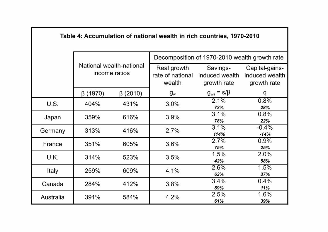
Table 4 presents our results on the decomposition of 1970-2010 national wealth accumulation

into saving and capital gains e↵ects.41 The main finding is that new savings explain the largest

part of wealth accumulation, but that there is also a clear pattern of positive capital gains. Take

the U.S. case. National wealth was equal to 404% of national income in 1970, and is equal to

431% of national income in 2010. National wealth has grown at an average real rate gw = 3.0%

per year. On the basis of national saving flows alone, we find that wealth would have grown

at rate gws = 2.1% per year only. We conclude that the residual capital-gains-induced wealth

growth rate q = (1+ gw)/(1+ gws)�1 has been equal to 0.8% per year on average. New savings

explain 72% of the accumulation of national wealth in the U.S. between 1970 and 2010, while

residual capital gains explain 28%.

Just like in the U.S., new savings also appear to explain around 70-80% of 1970-2010 national

wealth accumulation in Japan, France, and Canada, and residual capital gains 20-30%. Capital

gains are larger in the U.K., Italy, and Australia.

38See, e.g., Hayashi (1986) on Japanese tastes for bequest.39The e↵ect of the rise of life expectancy on saving behavior is unclear. In theory, rising life expectancy may

have contributed to pushing saving rates upward, but in practice the level of annuitized wealth seems to berelatively low in a number of rich countries. In France for instance, annuitized wealth represents less than 3%of aggregate private wealth (see Piketty 2011, Appendix A p.37-38), suggesting that this channel does not playan important role in the rise of the wealth-income ratio. In countries with less generous pay-as-you-go pensionsystems, annuitized wealth can be as large as 10%-20% of aggregate private wealth.

40See Appendix Figures A122 and A123. Note that in some countries a large fraction of private savings isabsorbed by government deficits (more than one third in Italy over the 1970-2010 period).

41Here we only show the multiplicative decompositions of national wealth. The additive decompositions yieldsimilar conclusions; see Appendix Table A101. Additive and multiplicative decompositions of private wealth arepresented in Appendix Table A111b.

22

The capital gains we compute are obtained as a residual, and so may reflect measurement

errors in addition to real valuation e↵ects.42 There are two main possible issues. First, it

is entirely possible that national saving flows are substantially under-estimated because they

do not include research and development expenditure. To address this concern, we have re-

computed our wealth accumulation equations using saving flows that include R&D. Even after

we include generous estimates of R&D expenditure, in many countries the 2010 observed levels

of national wealth are still significantly larger than those predicted by 1970 wealth levels and

1970-2010 saving flows alone (Figure 7a).43 Take the case of France: predicted national wealth

in 2010 – on the basis of 1970 initial national wealth and cumulated 1970-2010 national saving

including R&D – is equal to 491% of national income, while observed national wealth is equal

to 605%. We have the equivalent of over 100% of national income in “excess wealth”.44

Second, we might somewhat underestimate the value of public assets at the beginning of the

period in countries like the U.K., France and Italy. Part of the capital gains we measure might

simply correspond to the fact that private agents have acquired privatized assets at relatively

cheap prices. From the viewpoint of households this is indeed a capital gain, but from a national

wealth perspective it is a pure transfer from public to private hands, and it should be neutralized

by raising the level of 1970 wealth. Whenever possible, we have attempted to count government

assets at equivalent market values throughout the period (including in 1970), but we might still

slightly under-estimate 1970 government wealth levels.

In the end, in our preferred specification that includes generous R&D expenditure in saving

flows, capital gains account for about 40% on average of the total 1970-2010 increase in �, and

42In the Appendix, we have checked that the pattern of capital gains residuals we find is highly correlatedwith capital gains on listed equities and housing coming from available asset price indexes (see Figures A143 toA157). Note that the capital gains inferred from our wealth decomposition exercises are structurally lower thanthose coming from equity price indexes, for a good reason. A substantial fraction of national saving takes theform of corporate retained earnings (see Table 3) and these earnings generate structural capital gains in equitymarkets. Should we exclude retained earnings from saving in the wealth accumulation equation, then we wouldsimilarly find much larger residual capital gains (see Appendix Table A105). Such capital gains, however, wouldbe spurious, in the sense that they correspond to the accumulation of earnings retained within corporations tofinance new investment (thereby leading to rising stock prices), rather than to a true relative price e↵ect.

43R&D has been included in investment in the latest SNA guidelines (2008), but this change has so far onlybeen implemented in Australia. The computations reported in Figures 7a-7b include generous estimates of R&Dinvestment based on the level of R&D expenditure observed in the U.S. satellite account over the 1970-2010period (see Appendix A.5.2 for a detailed discussion).

44Saving flows might be under-estimated for reasons other than R&D. Given the limitations of nationalaccounts (in particular regarding the measurement of depreciation, which is discussed in Appendix SectionA.1.2.), this possibility certainly cannot completely be ruled out. One would need, however, large and systematicerrors to account for the amount of excess wealth we find.

23

saving for about 60%, with a lot of heterogeneity across countries.45

How can we explain the substantial capital gains we find? As we shall see below, housing

and stock market capital gains in the U.K. and France since the 1970s-1980s can be understood

as the outcome of a long run asset price recovery. Asset prices fell substantially during the

1910-1950 period, and have been rising regularly ever since 1950. There might, however, have

been some overshooting in the recovery process, particularly in housing prices. Four of the

countries with the largest capital gains – UK, France, Italy, Australia – have by far the largest

level of housing wealth in our sample: over 300% of national income in 2010, a level that was

only attained by Japan around 1990. So it is tempting to conclude that part of the capital gains

we measure owe to abnormally high real estate prices in 2010.

To a large extent, the housing bubble explanation for the rise of wealth-income ratios is

complementary to the real explanation. In countries like France and Italy, savings are su�ciently

large relative to growth to generate a significant increase in the wealth-income ratio. Given the

values taken by s and g over the 1970-2010 period, and given the steady-state formula � = s/g,

the wealth-income ratios � observed in 1970 were too low and had to increase. If in addition

households in these countries have a particularly strong taste for domestic assets like real estate

(and/or do not want to diversify their portfolio internationally as much as they could) then

maybe it is not too surprising if this generates high upward pressure on housing prices.

There is one interesting exception to the general pattern of positive capital gains: Germany.

Given the relatively large saving flows and low growth rates in 1970-2010, we should observe

more wealth in 2010 than 400% of national income. According to our estimate that includes

R&D expenditure in saving flows, “missing wealth” in Germany is of the order of 50-100% of

national income (Figure 7a). German statisticians might over-estimate saving and investment

flows, or under-estimate the current stock of private wealth, or both.

Yet another possibility is that Germany has not experienced any asset price recovery so

far because the German legal system still today gives important control rights over private

assets to stakeholders other than private property owners. Rent controls, for instance, may

have prevented the market value of real estate from increasing as much as in other countries.

Voting rights granted to employee representatives in corporate boards may similarly reduce the

market value of corporations.46 Germans might also have less taste for expensive capital goods

45See Appendix A.5.2 and Appendix Table A99.46Whether this is good or bad for productive e�ciency is a complex issue which we do not address in this

24

(particularly housing goods) than the French, the British and the Italians, maybe because they

have less taste for living in a large centralized capital city and prefer a more polycentric country,

for historical and cultural reasons. With the data we have at our disposal, we are not able to

put a precise number on each explanation.

Last, it is worth noting that when we compute a European average wealth accumulation

equation – by taking a weighted average of Germany, France, U.K. and Italy – then capital

gains and losses seem to partly wash out (Figure 7b). Europe as a whole has less residual

capital gains than the U.K., France, and Italy, thanks to Germany. Had we regional U.S.

balance sheets at our disposal, maybe we would find regional asset price variations within the

U.S. that would not be too di↵erent from those we find in Europe. So one possibility is that

substantial relative asset price movements happens permanently within relatively small national

or regional economic units, but tend to correct themselves at more aggregate levels. German

asset prices might rise in the near future and fall in other European countries.

4.5 Domestic capital vs. foreign wealth

So far we analyzed the accumulation of wealth without paying attention to the composition of

wealth portfolios, and in particular irrespective of whether wealth is invested domestically or

abroad. National wealth, as we have seen, can be written as the sum of domestic capital and net

foreign wealth.47 The basic fact to have in mind is that net foreign wealth – whether positive

or negative – has been a relatively small part of national wealth in rich countries throughout

the 1970-2010 period (see Figure 6).

Despite this fact, external wealth has turned out to play an important role in the general

evolution of wealth-income ratios. First, Japan and Germany have accumulated sizable positive

net foreign positions in the 1990s-2000s, due to their large trade surpluses. In the early 2010s,

both countries own the equivalent of between 40% and 70% of national income in net foreign

assets. Although Japan’s and Germany’s net foreign positions are still substantially smaller

paper (at first sight, low equity values do not seem to prevent German firms from producing good products). Inthis “stakeholder” view of the firm, the market value of corporations can be interpreted as the value for capitalowners, while the book value can be interpreted as the value for all stakeholders. Both views have their merits.See Appendix for further discussion.

47Remember that a country’s net foreign wealth is equal to its gross foreign assets (assets owned by residentsin the rest of the world) minus its gross foreign liabilities (domestic assets owned by rest-of-the-world residents).Domestic capital is national wealth minus net foreign wealth, i.e. is equal to the market value of all domesticcapital assets located in the home country, whether they are owned by the personal, government, or corporatesector, or by the rest of the world (see below for a decomposition between housing and other capital goods).

25

than the positions reached by the U.K. and France around 1900-1910, they are starting to be

substantial. And the German position is rising fast. As a result, in Japan and Germany, the

rise in net foreign assets represents more than a quarter of the total rise of the national wealth-

national income ratio (Table 5). In most of the other countries in our database, by contrast, net

foreign positions are currently slightly negative – typically between -10% and -30% of national

income – and have been declining. For those countries, the rise in the domestic capital-output

ratio has been larger than the rise in the national wealth-income ratio. One caveat is that

the o�cial net foreign asset positions do not include the sizable assets held by a number of

rich country residents in tax havens. In all likelihood, including these assets would turn the

rich world’s total net foreign asset position from negative to positive. The improvement would

probably be particularly large for Europe (Zucman, 2013).

Second, there has been a huge rise in the gross foreign positions of countries since the 1970s.

A significant share of each country’s domestic capital is now owned by other countries. The

rise in cross-border positions is highly significant everywhere – it is spectacular in Europe, a

bit less so in the world’s largest economies, the U.S. and Japan.48 One implications is that

capital gains and losses on foreign portfolios can be large and volatile over time and across

countries. And indeed, we find that foreign portfolios have generated large capital gains in the

U.S. (but also the U.K. and Australia) and significant capital losses in some other countries

(Japan, Germany, France). Strikingly, in Germany virtually all capital losses at the national

level can be attributed to foreign assets (Table 6). In the U.S., net capital gains on cross-border

portfolios represent one third of total capital gains at the national level, and the equivalent of

the total rise in the U.S. national wealth-national income ratio since 1970.49

4.6 Housing vs. other domestic capital goods

Last, we present decomposition results for housing versus other domestic capital assets.

48In 2010, gross assets held in France by the rest of the world amount to about 310% of national income,while gross assets held by French residents in the rest of the world amount to about 300% of national (hence anegative position of about -10%, in the o�cial data). For the U.S., gross foreign assets amount to about 120%of national income, and gross liabilities to about 100% of national (hence a negative position equal to about-20%). For detailed series, see Appendix figures A39-A42.

49Our results on the net capital gains on U.S. external wealth are consistent with the findings of Gourinchasand Rey (2007). What we add to this line of work is a global macro perspective that includes the accumulationof both domestic and foreign capital. Note that we include all “other volume changes” in saving flows butexclude R&D from saving. We provide detailed accumulation results isolating saving, “other volume changes”,and capital gains in the country-specific tables of the Appendix.

26

The accumulation of housing wealth has played a large role in the total accumulation of

domestic capital, but with significant variations between countries. In the U.K., France and

Italy, the rise in domestic capital-national income ratios (or domestic capital-output ratios) is

almost entirely due to the rise of housing (Table 7). In Japan, housing represents less than half

of the total rise of domestic capital – and an even smaller proportion of the total rise of national

wealth, given the large accumulation of net foreign assets.50

In most countries, other domestic capital goods have also contributed to the rise of national

wealth, in particular because their market value has tended to increase. Tobin’s Q ratios

between market and book value of corporations were much below 1 in the 1970s and are closer

to 1 (and at times above 1) in the 1990s-2000s.51 But there are again interesting cross-country

variations. Tobin’s Q is very low in Germany: is has remained well below 1 (typically around

0.5), contrary to the U.K. and the U.S. One interpretation is the “stakeholder e↵ect” described

above: shareholders of German companies do not have full control of company assets – they share

their voting rights with workers’ representatives and sometime regional governments – which

might push Q below 1.52 Yet another possibility is that some of the variations in Q reflect data

limitations. Quite puzzlingly, indeed, in most countries Q appears to be structurally below 1,

although intangible capital is imperfectly accounted for, which in principle should push it above

1. Part of the explanation may be that the book-value of corporations – corporate assets as

measured by statisticians using the perpetual inventory method – tends to be over-estimated in

national accounts. This is another area in which existing statistics might need to be improved.

5 Wealth-income ratios in rich countries 1870-2010

It is impossible to properly understand the rise of wealth-income ratios in rich countries in the

recent decades without putting the 1970-2010 period into a longer historical perspective. As we

50One caveat is that the frontier between housing and other capital goods is not always entirely clear. Some-times the same buildings are reallocated between housing and o�ces, and housing services can be provided byhotels and real estate companies. Also, the various countries do not always use the same methods and concepts(e.g., in Japan, tenant-occupied housing is partly counted in other domestic capital, and we could not fullycorrect for this). This is an area where progress still needs to be made. Appendix A.9 pinpoints the key areasin which we believe national accounts could be improved.

51See Appendix Figure A92. Note, however, that because of the general increase in corporate capital, book-value national wealth (expressed as a fraction of national income) has increased almost as much as market-valuenational wealth (see Appendix figure A25).

52In Germany, book-value national wealth is substantially above market-value national wealth (about 5 yearsof national income instead of 4 years). The opposite occurs in the U.K.

27

have seen, a significant part of the rise of � since the 1970s is due to capital gains: about 40%

on average, with large di↵erences between countries. The key question is the following: is this

due to a structural, long-run rise in the relative price of assets (caused for instance by uneven

technical progress), or is it a recovery e↵ect? Our conclusion is that it is mostly a recovery

e↵ect. The capital gains observed during the 1970-2010 period largely seem to compensate the

capital losses observed during earlier parts of the 20th century.

We have reached this conclusion by analyzing the evolution of wealth-income ratios over the

1870-2010 period. Due to data limitations, our long term analysis is restricted to four countries:

the U.S., the U.K., Germany and France. The key descriptive statistics are the following.

For the three European countries, we find a similar U-shaped pattern: today’s private wealth-

national income ratios appear to be returning to the high values observed in 1870-1910, namely

about 600%-700% (Figure 2 above). For the U.S., the U-shaped pattern is much less strong

(Figure 4 above). In addition, European public wealth-national income ratios have followed an

inverted U-curve over the past century.53 But the magnitude of the pattern for public wealth

is very limited compared to the U-shape evolution of private wealth, so that European national

wealth-income ratios are strongly U-shaped too. Last, in 1900-1910, European countries held

a very large positive net foreign asset position – around 100% of national income on average.

Interestingly, the net foreign position of Europe has again turned (slightly) positive in 2000-2010,

when the national wealth-income ratio again exceeded that of the U.S. (Figure 8).

Starting from this set of facts, and using the best historical estimates of saving and growth

rates, we have estimated detailed 1870-2010 wealth accumulation equations. As Table 8 shows,

the total accumulation of national wealth over this 140-year-long period seems to be well ac-

counted for by saving flows. In order to fully reconcile the stock and flow data, we need a small

residual capital gain for the U.S., France and the U.K., and a small residual capital loss for

Germany. But in all cases saving flows account for the bulk of wealth accumulation: capital

gains seem to wash out in the long run.54

Looking at each sub-period, we find in every European country a strong U-shaped relative

53Net public wealth was significantly positive (around 100% of national income) during the 1950s-1970s, dueto large public assets and low debt. Since then, public wealth has returned to the low level observed on the eveof World War 1.

54These results are robust to a wide range of specifications. Appendix Tables A108 to A137 present the com-plete decomposition results, for each country and sector of the economy, for both the additive and multiplicativemodels.

28

capital price e↵ect. In the U.K., for example, we find a negative rate of real capital losses equal

to -1.9% per year between 1910 and 1950, followed by real gains of +0.9% per year between 1950

and 1980 and 2.4% between 1980 and 2010 (Table 9). The pattern is similar for France. In these

two countries, there seems to have been a slight over-shooting in the recovery process, in the

sense that the total cumulated relative asset price e↵ect over the 1910-2010 period appears to

be somewhat positive (+0.2% per year in the U.K., +0.3% in France). In Germany, by contrast,

the recovery is yet too come (-0.8% between 1910 and 2010).

We emphasize that the imperfections of our data do not allow us to put a precise number on

asset over- or undervaluation in 2010. In any multi-sector model with uneven technical change

between capital and consumption goods, one should expect capital gains and losses that could

vary between countries (for instance depending on comparative advantage). The residual capital

gains/losses we estimate might also reflect measurement issues: 1870-2010 saving flows might be

somewhat underestimated in the U.K. or France and overestimated in Germany. At a modest

level, our point is simply that the one-good capital accumulation model seems to do a relatively

good job in the long run, and that the stock and flow sides of historical national accounts are

roughly consistent with one another – a result we already find quite remarkable.

Table 10 decomposes the huge decline in wealth-income ratios that occurred in Europe

between 1910 and 1950. In the U.K., war destructions play a negligible role – an estimated 4%

of the total decline in �. Low national saving during this period accounts for 46% of the fall in �

and negative valuation e↵ects (including losses on foreign portfolios) for the remaining 50%. In

France and Germany, cumulated physical war destructions account for about one quarter of the

fall in �. Low national saving and real capital losses each explain about half of the remaining

three quarters. Interestingly, the private wealth-national income ratio has declined less in the

U.K. than in France and Germany between 1910 and 1950, but the reverse holds for the national

wealth-income ratio (due to the large negative U.K. public wealth around 1950).55

The U.S. case is again fairly di↵erent from that of Europe. The fall of � during the 1910-1950

period was more modest, and so was the recovery since 1950. Regarding capital gains, we find

in every sub-period a small but positive relative price e↵ect. The capital gain e↵ect becomes

bigger in the recent decades and largely derives from the U.S. foreign portfolio – it seems too

big to be accounted for by underestimated saving and investment flows.

55U.K. net public wealth then turned positive during the 1950s-1960s. See Appendix figure A16 and A22.

29

6 The changing nature of national wealth, 1700-2010

6.1 The changing nature of wealth in Old Europe

What do we know about the evolution of wealth-income ratios prior to 1870? In the U.K. – the

country with the most comprehensive historical balance sheets – the national wealth-national

income ratios appears to have been approximately stable during the 18th and 19th centuries

– around 600-700%, or possibly somewhat higher (Figure 3 above). In France, where a large

number of historical national wealth estimates were also established during those two centuries,

the picture is similar (Figure 9).

We should make clear that the raw data sources available for the 18th-19th centuries are

insu�cient to precisely compare the levels of wealth-income ratios between the two countries

or between the various sub-periods. But the general pattern definitely seems to be robust.

All available estimates, coming from many di↵erent authors using independent methodologies,

provide the same orders of magnitude. National wealth always seems to be between 6 and 8

years of national income (usually around 7 years) from 1700 to 1914 in two countries, with no

obvious trend in the long run.

Strikingly, the wealth-income ratio around 2010 is now relatively close to what it was in

the 18th centuries in both the U.K. and France, in spite of considerable changes in the nature

of wealth. The general picture is relatively straightforward. The value of agricultural land –

including land improvement of all sorts – was between 4 and 5 years of national income in the

U.K. and the France in the early 18th centuries, and is now less than 10% national income

in both countries. But land has been replaced by other forms of capital – housing and other

domestic capital (o�ces, machines, patents, etc.) – to such an extent that the wealth-income

ratio appears to be almost as high today as three hundred years ago. In the long run, the decline

of the share of agricultural land in national capital mirrors that of the share of agriculture in

national income, from over two thirds in the 18th century to a few percent today – with a faster

and earlier historical decline in the U.K. The huge variations in the share of net foreign assets

in national wealth are also striking. Net foreign assets were virtually zero in the 18th century.

They reached very high levels in the late 19th and early 20th century – almost 2 years of national

income in the U.K. around 1910, over 1 year in France. Following the wars and the collapse of

the British and French colonial empires, they came back to virtually zero around 1950.

30

Why is it that wealth-income ratios were so high in the 18th-19th centuries, and why do they

seem to be approaching these levels again in the 21st century? A natural explanation lies in the

� = s/g steady-state formula. With slow growth, even moderate saving rates naturally lead to

large wealth-income ratios. Growth was low until the 18th-19th centuries, and is likely to be low

again in the 21st century as population growth vanishes, thereby potentially generating high

wealth-income ratios again.

This is probably an important part of the explanation. Unfortunately, data limitations

make it di�cult to evaluate the exact role played by alternative explanations, such as structural

capital gains and losses and changes in the value of natural resources (un-accumulated wealth).

The main di�culty is that pre-1870 estimates of saving and investment flows appear to be too

fragile to be used in wealth accumulation decompositions. Also, with very low growth – annual

growth rates were typically much less than 1% until the 18th century – it is clear than any small

error in the net-of-depreciation saving rate s can make a huge di↵erence in terms of predicted

steady-state wealth-income ratio � = s/g. In preindustrial societies where g ⇡ 0.5 � 1%,

whether the net saving rate is s = 5% or s = 8% is going to matter a lot. Historical estimates

suggest that there was substantial investment going on in traditional societies, including in the

rural sector. Annual spendings on land improvement (drainage, irrigation, a↵orestation etc.)

alone could be as large as 3-4% of national income. This suggests that a large fraction of total

agricultural land value in 18th century U.K. and France actually derived from past investment.

In all likelihood, the “pure land value” (i.e., the value of the pure natural resource brought

by land, before any investment or improvement, as it was discovered thousands of years ago,

at prehistoric times) was much less than 4 years of national income. Some estimates made in

the 18th century tend to suggest that it was around 1 year of national income.56 Saving and

investment series are unfortunately not su�ciently reliable to definitively address the question.

The residual “pure land” value could be less than 0.5 year, or up to 2 years of national income.

6.2 The nature of wealth: Old Europe vs. the New World

In order to make some progress on this question, it is useful to compare the value of land

in Old Europe (U.K., France, Germany) and in the New World. For the U.S., we have put

56See in particular the famous estimates by Thomas Paine (1795), who suggested in front of the FrenchNational Assembly to confiscate the “pure land” component of inheritance, which he estimated to be about 1year of national income. On saving and investment series covering the 18th-19th centuries, particularly for theU.K. and France, see data Appendix.

31

together historical balance sheets starting around 1770 (Figure 10). The robust finding, which

we also obtain with Canada, is that the value of agricultural land in the late 18th and early

19th centuries is much less in the New World – 1 to 2 years of national income – than in Old

Europe – 3 to 4 years.57 Part of the explanation could well be lower accumulated investment

and land improvement relative to economic and population growth in the New World (i.e., a

lower cumulated s/g ratio). However, available evidence suggests that the relatively low New

World wealth-income ratios can also be explained by a “land abundance” e↵ect. Land was so

abundant in the New word that its price per acre was low. The right model to think about

this e↵ect involves a production function with an elasticity of substitution lower than 1 between

land and labor – a necessary condition for the price e↵ect to dominate the volume e↵ect.

To see this, think of a two-good model of the form introduced in section 3.4 above. That is,

assume that the capital good solely consists of land and is in fixed supply: Vt = V . For the sake

of simplicity, assume that no land improvement is possible. The market value of land if given

by K = qV , where q is the price of land relative to the consumption good. The production

function Y = F (V, L) transforms capital input (land) V and labor input L into output Y .

Assume that F (V, L) is a CES function with elasticity �, and that there is zero productivity

and population growth.

Consider two countries 0 and 1 with similar technology and preferences. Assume that country

1 (America) has more land relative to labor than country 0 (Old Europe): V1/L1 > V0/L0. Then

one can easily see that country 1 will end up with lower land value (relative to income) than

country 0 (i.e., �1 < �0, with �1 = K1/Y1 = q1 ·V1/Y1 and �0 = K0/Y0 = q0 ·V0/Y0) if and only if

the elasticity of substitution � is less than one. This result directly follows from the fact that the

capital share ↵ is smaller in country 1 than in country 0 (i.e., ↵1 = FV ·V1/Y1 < ↵0 = FV ·V0/Y0)

if and only if � is less than one. The capital share is lower in the land-abundant country. Under

standard assumptions on preferences and equilibrium rates of return, this also implies that land

value is lower in the land-abundant country: �1 < �0.58

57For the long run evolution of wealth composition in Germany and Canada, see Appendix figures A46 andA47. The German pattern is close to that of the U.K. and France (except that the net foreign asset position ofGermany around 1900-1910 is less strongly positive than in the two colonial powers). The Canadian pattern isclose to that of the U.S. (except that net foreign asset position is strongly negative throughout the 19th centuryand much of the 20th century).

58With a dynastic utility model, the rate of return is set by the rate of time preference (r = ✓), so that�1 = ↵1/r < �0 = ↵0/r. With a bequest-in-the-utility-function model U(c, b) = c1�sbs, then the wealth-incomeratio is set by � = s/(1�s) (see section 3.4 above), so that the di↵erence in capital share entirely translates into adi↵erence in rates of return: r1 = ↵1/� < r0 = ↵0/�. However to the extent that the interest elasticity of saving

32

Intuitively, an elasticity of substitution � < 1 means that there is not much that one can do

with capital when there is too much of it. The marginal product of land falls to very low levels

when a few million individuals own an entire continent. The price e↵ect dominates the volume

e↵ect. It is exactly what one should expect to happen in a relatively low-tech economy where

there is a limited set of things that one can do with capital. At the opposite extreme, in a high-

tech economy where there are lots of alternative uses and forms for capital (a robot economy),

it is natural to expect higher elasticities of substitution, either closer to 1 (Cobb-Douglas) or

even larger than one (as we shall see below).

To summarize: part of the initial di↵erence in � between Europe and America in the 18th-

19th centuries seems to be due to a relative price e↵ect (due to land abundance) rather than to

a pure saving e↵ect (via the � = s/g formula). Both logic actually tend to reinforce each other:

the lower land prices and higher wage rates attract labor to the New World, implying very large

population growth rates and relatively low steady-state � = s/g ratios.59

The lower land values prevailing in America during the 1770-1860 period were to some

extent compensated by the slavery system. Land was so abundant that it was almost worthless,

implying that it was di�cult to be really rich by owning land. However, the landed elite could

be rich and control a large share of national income by owning the labor force. In the extreme

case where a tiny elite owns the entire labor force, the total value of the slave stock can in

principle be very large, say as large as 20 years of national income (assuming the labor share

is 100% of output and the rate of return is equal to 5%).60 In the case of antebellum U.S.,

the situation was less extreme, but the value of the slave stock was still highly significant. By

putting together the best available estimates of slave prices and the number of slaves, we have

s = s(r) is positive, this also implies �1 < �0. A similar intuition applies to the case with U(c, b) = c1�s�bs

(assuming positive population or productivity growth so as to obtain a well-defined steady-state � = s/g).59There is a large historical literature on the factor flows that characterized the 19th Atlantic economy. In

order to explain why both labor and capital flew to the New World, one needs to introduce a three-factorproduction function (see, e.g., Taylor and Williamson, 1994, and O’Rourke and Williamson, 2005). One couldalso argue that transatlantic di↵erences in land value (rural, urban and suburban) still matter today. Howeverthey go together with di↵erent tastes over housing in city centers versus suburban areas, so that it is di�cultto disentangle the various e↵ects. The fact that the bulk of 1870-2010 wealth accumulation is well explained byvolume e↵ects – both in Europe and in the U.S. – suggests that today’s di↵erences in pure land values are lesscentral than they used to be.

60With a one-good model and a Cobb-Douglas production function F (K,L) = K↵L1�↵, the market value �H

of the human capital stock (i.e., the value of the labor force from the viewpoint of a potential slave owner) isalways equal to (1 � ↵)/↵ times the non-human capital stock. If ↵ = 1/3, then �H = 2�. This is assumingthat the slave owner equates returns across all human and non-human assets. With a CES production functionF (K,L) = (a ·K ��1

� + (1� a) · L��1� )

���1 , we have �H = 1

a · �1/� � �.

33

come to the conclusion that the market value of slaves was between 1 and 2 years of national

income for the entire U.S., and up to 3 years of income in Southern states. When we add up the

value of slaves and the value of land, we obtain wealth-income ratios in the U.S. South which

are relatively close to those of the Old World. Slaves approximately compensate the lower land

values (Figures 11 and 12).

Needless to say, this peculiar form of wealth has little to do with “national” wealth and is

better analyzed in terms of appropriation and power relationship than in terms of saving and

accumulation. We view these “augmented” national balance sheets as a way to illustrate the

ambiguous relationship of the New world with wealth and inequality. To some extent, America

is the land of equal opportunity, the place where wealth accumulated in the past does not matter

too much. But at the same time, America is also the place where a new form of wealth and class

structure – arguably more extreme and violent than the class structure prevailing in Europe –

flourished, whereby part of the population owned another part.61

7 Capital-output ratios vs. capital shares

So far we have mostly focused on the evolution of wealth-income and capital-output ratios.

We now compare the long-run evolution of capital-output ratios and capital shares in order to

briefly discuss the changing nature of technology and the pros and cons of the Cobb-Douglas

approximation in the very long run.

The first basic fact is that capital shares did rise in rich countries during the 1970-2010

period, from about 15%-25% in the 1970s to 25%-35% in the 2000s-2010s, with large variations

over time and across countries (Figure 13). However they did not rise as much as national

wealth-national income and domestic capital-output ratios, so that the average of return to

wealth – which can be computed as rt = ↵t/�t – declined somewhat (Figure 14).62 Of course,

this decline is what one would expect in any model: when there is more capital, the rate of

return to capital must go down. The interesting question is whether it falls more or less than

the quantity of capital. According to our data it has fallen less, implying a rising capital share.

There are several ways to think about this piece of evidence. One can think of a model

61During the 1770-1860 period, slaves made as much as 15%-20% of total U.S. population (up to 40% inSouthern states). See Appendix Table US.3b.

62The results are robust to the various ways of taking into account government capital and interest paymentin these computations, which are discussed in Appendix A.7.5. The reader should have in mind that like all ourincome series, the capital shares displayed in Figure 13 are net of depreciation.

34

with imperfect competition and an increase in the bargaining power of capital (e.g., due to

globalization and increasing capital mobility). One can also think of a production function with

three factors – capital, high skill labor and low skill labor – where capital is more strongly

complementary with skilled than with unskilled labor. With a rise in skills, and possibly with

skill-biased technical change, it can easily generate a rising capital share.

Yet another – and more parsimonious – way to obtain the same result is a standard two-

factor, CES production function F (K,L) with an elasticity of substitution � > 1.63 Importantly,

the elasticity does not need to be hugely superior to one in order to account for the observed

trends. With an elasticity � around 1.2-1.6, a doubling of capital-output ratio � can lead to a

large rise in the capital share ↵. With large changes in �, one can obtain substantial movements

in the capital share with a production function that is only moderately more flexible than the

standard Cobb-Douglas function. For instance, with � = 1.5, the capital share rises from

↵ = 28% to ↵ = 36% if the wealth-income ratio jumps from � = 2.5 to � = 5, which is roughly

what has happened in rich countries since the 1970s. The capital share would reach ↵ = 42%

in case further capital accumulation takes place and the wealth-income ratio attains � = 8. In

case the production function becomes even more flexible over time (say, � = 1.8), the capital

share would then be as large as ↵ = 53%.64

We do not claim that this scenario will necessarily happen. Our point is simply that it

cannot be excluded. Constant capital-output ratios and capital shares are more of a belief than

a well-grounded fact. Capital-output ratios have no strong reason to stay constant: s and g vary

for all sorts of reasons over time and across countries, so it is natural to expect � = s/g to vary

63One can of course combine the various possible explanations. Karabarbounis and Neiman (2013) for instanceuse a two-goods model in which there is a decline in the relative price of investment. As a result, firms shift awayfrom labor toward capital, and with an elasticity of substitution � larger than 1 the capital share ↵ increases.As the two-goods model we apply in section 6.2. to 19th century U.S. and Europe illustrates, when the relativeprice of investment is lower (e.g., lower land values) and � > 1, the wealth-income ratio has to be higher.Thus, the explanation for the rise in ↵ put forward by Karabarbounis and Neiman (2013) is consistent with ourfindings of rising �. The di↵erence is that we do not need a two-goods model to account for the rise in ↵: inany one-good model, when g decreases (while s remains the same so that � increases) and � > 1, ↵ has to rise.In the real world, both forces (lower g and declining relative price of some capital goods) probably play a rolein the dynamics of ↵, so that the two explanations should be seen as complementary. One problem, however,with the declining relative price of capital story is that while the price of corporate tangible fixed assets mayhave declined, taking a broader view of capital we actually find a positive relative price e↵ect over 1970-2010(see section 4). This could be due to a positive price e↵ect for land, foreign, and R&D assets, which are notincluded in standard measures of the relative price of capital.

64In a perfectly competitive model with Y = F (K,L) = (a ·K ��1� + (1� a) · L��1

� )�

��1 , the rate of return is

given by r = FK = a · ��1/� (with � = K/Y ), and the capital share is given by ↵ = r · � = a · � ��1� . With

a = 0.21 and � = 1.5, ↵ goes from 28% to 36% and 42% as � rises from 2.5 to 5 and 8. With � = 1.8, ↵ rises to53% if � = 8.

35

widely. Relatively small departures from standard Cobb-Douglas assumptions then imply that

the capital share ↵ = r · � can also vary substantially. In our view, it is natural to imagine that

� was possibly much less than 1 in the 18th-19th centuries and became significantly larger than

1 in the 20th-21st centuries. One expects a higher elasticity of substitution in more diversified

economies where capital can take many forms.65

Taking a very long run perspective on the evolution of factor shares, there seems to be

evidence – both in the U.K. and France – that the capital share was somewhat larger in the

18th-19th centuries (say, around 40%) than it is in the early 21st century (about 30%), despite

the recent rise. Will capital shares return to their 18th-19th century levels? The capital-output

ratio � is still somewhat lower today than what it used to be in the distant past. So one

possibility is that the capital share ↵ will slowly return to about 40% as � keeps increasing

in the coming decades – consistent with an elasticity of substitution larger than 1. However,

it could also be that the labor exponent in the production function has declined structurally

since the 18th-19th centuries, because of the rise of human capital. Over time, human inputs

may have become relatively more important than non-human capital inputs in the production

process. With the data we have at our disposal, we are not able to say. The long-run U.K. and

French data, however, suggest that if such a “rise of human capital” happened, it was probably

relatively modest.

We stress that our discussion of capital shares and production functions should be viewed

as merely exploratory and illustrative. In many ways, it is more di�cult to measure capital

shares ↵ than wealth-income ratios �. The measurement of ↵ – and therefore of the average

rate of return r = ↵/� – is complicated by self-employment and tax optimization behavior of

business owners (a growing concern in a number of countries), by the measurement of housing

product (which is not fully homogenous internationally), and also by the problem of “informal”

financial intermediation. National accounts deduct from the return to capital the costs of formal

intermediation services (provided by banks and real estate agents), but do not deduct the time

spent by capital owners to manage their portfolios, to spot the right investment opportunities,

and so on. Such costs are di�cult to measure, and might well vary over time. In particular,

they might be larger in fast growing economies rather than in the stagnant, rural economies

65The fact that the capital share ↵ was historically low in the mid-20th century (when � was also low) canalso be viewed as evidence for � > 1. Indeed, ↵ and � move in the same direction if � > 1, and in oppositedirections if � < 1.

36

of the 18th century. For this reason, we may tend to over-estimate average rates of return

to capital when we compute them using national accounts capital income flow series (via the

r = ↵/� formula), especially in high-growth economies. In this paper, we have tried to show

that an alternative way to address the issue of the relative importance of capital and labor in

the economy is to study the evolution of � rather than the evolution of ↵ – which so far has

been the focus of most of the attention. Ideally, both evolutions need to be analyzed together.

8 Directions for future research

Our analysis could be extended in various ways. First, it would be interesting to study wealth-

income ratios at the world level. Throughout the 1870-2010 period, the top eight developed

economies analyzed in this paper represent between one half and three quarters of world output.

By making plausible assumptions about the evolution of other countries’ wealth-income ratios,

we have estimated the evolution of the world wealth-income ratio between 1870 and 2010.

Unsurprisingly, we find a spectacular U-shaped pattern (Figure 16).66 The exact levels are

approximate, but the general shape appears to be robust. Prior to World War 1, the world

wealth-income ratio was high and rising. Europe made about half of world output around 1900-

1910 and had a high wealth-income ratio; � was rising in the U.S. and other parts of the world.

The world ratio then fell abruptly during the 1910-1950 period. According to our estimates,

it has been recovering since then and is currently approaching its 1910 nadir. Around 75% of

the 1990-2010 rise in the world wealth-income ratio (from about 400% to about 450%) is due

to Europe and Japan, while China only accounts for about 15%. From a global perspective,

therefore, capital accumulation in rich countries is probably a much more important determinant

of the decline in the global return to capital than the large Chinese savings.67

We also report on Figure 16 one possible evolution of the wealth-income ratio in 2010-2100.

This projection is based upon specific and uncertain assumptions about the future. We take the

projected population growth rates from the U.N. central scenario (with near zero or negative

66See Appendix Table A8 for the detailed computations and assumptions behind Figure 16. Note that thenational wealth-national income ratio is less strongly U-shaped than the private wealth-national income ratio,due to the high level of global public assets in the 1950s-1970s.

67The increase in the net foreign asset position of China (from 0 to about 30% of national income) has beeneven smaller than the rise of China’s � (from about 200% to 400% of national income). However, to the extentthat China’s foreign saving is mostly invested in the U.S. and that national capital markets are segmented, theChina-U.S. capital flows might account for a substantial fraction of the decline in the U.S. return to capital.

37

population growth pretty much everywhere after 2050, except in Africa). We assume rapid

convergence of emerging countries (at current pace) and stabilization of per capita growth rates

at relatively low levels in frontier economies (1.4%). Last, we assume that saving rates will

stabilize around 10-12% of national income. If this happens, then the world wealth-income

ratio � will keep rising to about 600-700% by 2070-2100, i.e. approximately the same level as

Europe in the 18th-19th centuries. Needless to say, this is only one possible scenario. Much

will depend on the evolution of fertility behavior, life expectancy, innovation, the shape of the

production function (� > 1 or < 1), and the various psychological and economic motives for

saving.68 Our bottom line is simply that with low growth there are strong and powerful economic

forces pushing toward high wealth-income ratios in the global economy of the 21st century, just

like in the low growth societies of the past.

Next, it would be interesting to include individual-level wealth inequality in the analysis.

In this paper, we have emphasized the importance of aggregate wealth-income ratios and net

foreign wealth positions, i.e. inequality of wealth between countries. However there is evidence –

for example from Forbes’ global billionaires list – that the evolution of wealth inequality between

individuals is also quite spectacular (possibly even more). Over the past 20-30 years, the very

top of the world wealth distribution seems to have been rising at a rate that is substantially

above that of average wealth – which is itself substantially above the growth rate of per capita

income and output, given the rise in global �. One explanation could be that the slowdown of

growth can contribute to both a rise of the aggregate wealth-income ratio and to an increase of

wealth inequality. Indeed, in any dynamic wealth accumulation model with heterogeneity and

random multiplicative shocks, the steady-state variance and inverted Pareto coe�cient is an

increasing function of the r�g di↵erential between the net-of-tax rate of return and the growth

rate of the economy (see, e.g., Atkinson, Piketty and Saez, 2011).

Last, we plan to extend our analysis to investigate the evolution of the share of inherited

wealth in aggregate wealth. The return of high wealth-income ratios does not necessarily imply

the return of inheritance. In case wealth is distributed in a relatively egalitarian manner and

mostly derives from lifecycle saving, then one can have high and rising � with no corresponding

68Private saving rates around s =10-12% are in line with what we observe in rich countries – particularlyEurope and Japan – in recent decades, so it makes sense to use such values in our benchmark scenario. Howeverif we include government dissaving then national saving rates in rich countries are substantially lower than 10-12% and are on a declining trend, see Appendix Figures A96 to A103. It is also possible that saving rates willeventually react more strongly than expected to a decline in rates of return.

38

rise in inheritance. To see this, observe that the annual flow of inheritance, expressed as a

proportion of national income, which we note byt, can be decomposed as the product of three

terms: byt = µt ·mt ·�t (where �t is the aggregate-wealth income ratio, mt is the annual mortality

rate, and µt is the ratio between average wealth at death and the average wealth of the living).

With pure lifecycle wealth, µt = 0, so that byt = 0, irrespective of how large �t might be.

In the case of France, the long-run U-shaped pattern for the inheritance flow byt actually

turns out to be even more spectacular than the U-shaped pattern observed for �t, due to the fact

that µt has also followed a marked U-curve. The relative wealth of the elderly was historically

low in the postwar period, so that there was not much to inherit in the 1950s-1960s (Piketty,

2011). However this certainly does not imply that the same evolution applies everywhere.

As we have seen, there are large variations in the quantity of wealth that di↵erent countries

accumulate, so it is natural to expect large di↵erences in the importance of inherited wealth.

The historical series available so far regarding the inheritance flow are too scarce to reach

firm conclusions on this important issue. Existing estimates suggest that the French U-shaped

pattern also applies to Germany (Schinke, 2012), and to a lesser extent to the U.K. (Atkinson,

2012) and the U.S. (see Piketty and Zucman, 2013, for a survey). Cross-country variations

could be due to di↵erences in pension systems and the share of private wealth that is annuitized

and therefore non transmissible. From a theoretical perspective, however, it is unclear why

there should be much crowding out between lifecycle wealth and transmissible wealth in an

open economy: any extra pension wealth should be invested abroad. It could be that there are

di↵erences in tastes for wealth transmission across countries. Wealthy individuals in the U.K.

and in the U.S. may have less taste for bequest than in France and Germany.69 But there are

also important data problems that could partly explain why the rise of the inheritance flow

appears to be more limited in some countries than in others. Wealth surveys tend to vastly

underestimate inheritance receipts, not to mention inter vivos gifts, which play a large role

in the recent French and German evolution (and which can only be properly measured with

administrative data). All of this raises important challenges for future research.

69One can interpret the lower � = s/g in the U.S. in terms of lower bequest taste: with higher populationgrowth and the same bequest taste (per children) as in Europe, the U.S. should save more. However a large partof U.S. population growth historically comes from migration, so this interpretation cannot be fully accurate.

39

ReferencesAtkinson, Anthony B., “Wealth and Inheritance in Britain from 1896 to the Present,” Work-

ing paper, 2012.

Atkinson, Anthony B., Thomas Piketty and Emmanuel Saez, “Top Incomes in the

Long Run of History,” Journal of Economic Literature, 2011, vol.49(1), pp.3-71.

Azmat, Ghazala, Alan Manning, and John Van Reenen, “Privatization and the Decline

of Labour’s Share: International Evidence from Network Industries,” Working paper, 2011.

Babeau, Andre, “The Macro-economic Wealth-Income Ratio of Households”, Review of In-

come and Wealth, 1983, vol.29(4), pp.347-370.

Barro, Robert J., “Economic Growth in a Cross Section of Countries”, Quarterly Journal of

Economics, 1991, vol.106(2), pp.407-443.

Boisguillebert, Pierre, Le detail de la France, Paris, 1695, 215p. Reprinted in E. Daire,

Economistes financiers du 18 e siecle, Paris: Guillaumin, 1843.

Bowley, Arthur L., The Change in the Distribution of National Income, 1880–1913, Oxford:

Clarendon Press, 1920.

Carroll Christopher D., “Why Do the Rich Save so much?”, in Does Atlas Shrug? The

Economic Consequences of Taxing the Rich, J. Slemrod ed., Harvard University Press, 2000.

Carroll Christopher D., Jody Overland and David N. Weil, “Saving and Growth with

Habit Formation,” American Economic Review, 2000, vol.90(3), pp.341-355.

Caselli, Francesco and James Feyrer, “The Marginal Product of Capital,” Quarterly Jour-

nal of Economics, 2007, vol.122(2), pp.535-568.

Colquhoun, Patrick, A Treatise on the Wealth, Power and Resources of the British Empire,

London, 1815, 561p.

Colson, Clement, Cours d’economie politique, Paris: Gauthier-Villars, 1903, 1918, 1927 (sev-

eral editions).

Davies, James B., Susanna Sandstrom, Anthony Shorrocks and Edward N. Wol↵

“The Level and Distribution of Global Household Wealth,” Economic Journal, 2010, vol.121,

pp.223-254.

Denison, Edward F., The Sources of Economic Growth in the United States and the Alter-

natives Before Us, New York: Committee for Economic Development, 1962, 308pp.

Domar, Evsey “Expansion and Employment,” American Economic Review, 1947, vol.37(1),

pp.34-55.

Eisner, Robert, “Capital Gains and Income: Real Changes in the Value of Capital in the

United States, 1946-77”, pp.175-346, in The Measurement of Capital, Dan Usher, ed., University

of Chicago Press, 1980.

Ellis, Luci and Kathryn Smith, “The Global Upward Trend in the Profit Share,” BIS

working paper 231, July 2007, 29p.

Feinstein, Charles, “Capital Formation in Great Britain, 1760-1860,” in The Cambridge Eco-

nomic History of Europe, vol.7, Part 1, Chapter 2, Cambridge: Cambridge University Press,

1978, pp.28-96.

40

Foville, Alfred de, “The Wealth of France and of Other Countries,” Journal of the Royal

Statistical Society, vol.56(4), 1893, pp.597-626.

Gale, William G., and John Sabelhaus, “Perspectives on the Household Saving Rate,”

Brookings Papers on Economic Activity, 1999(1), 1999, pp.181-224.

Gi↵en, Robert, The Growth of Capital, London, 1889, 169p.

Goldsmith, Raymond W., Comparative National Balance Sheets: A Study of Twenty Coun-

tries, 1688-1978, Chicago: The University of Chicago Press, 1985, 353p.

Goldsmith, Raymond W., Pre-Modern Financial Systems, Cambridge: Cambridge Univer-

sity Press, 1991, 348p.

Gourinchas, Pierre-Olivier and Helene Rey, “From World Banker to World Venture Capi-

talist: The U.S. External Adjustment and the Exorbitant Privilege,” in G7 Current Account Im-

balances: Sustainability and Adjustment, Richard Clariada (ed), Chicago: University of Chicago

Press, 2007, pp.11-66.

Gourinchas, Pierre-Olivier and Helene Rey, “External Adjustment, Global Imbalances,

Valuation E↵ects,” forthcoming in Gita Gopinath, Elhanan Helpman and Kenneth Rogo↵ (eds)

Handbook of International Economics, vol.4, 2013.

Harrod, Henry, “An Essay in Dynamic Theory,” Economic Journal, 1939, vol.49(193), pp.14-

33.

Hayashi, Fumio, “Why is Japan’s Saving Rate so Apparently High?,” in Fischer S. (ed.),

NBER Macroeconomics Annual, 1986, vol.1, pp.147-234.

Hel↵erich, Karl, Deutschlands Volkswholhstand, 1888-1913, Berlin: G. Stilke, 1913, 164p.

(second edition, 1915).

Jones, Charles I. and Paul M. Romer, “The New Kaldor Facts: Ideas, Institutions, Pop-

ulation, and Human Capital,” American Economic Journal: Macroeconomics, 2010 vol.2(1),

pp.224-245.

Jorgenson, Dale W. and Zwi Griliches, “The Explanation of Productivity Change,” Review

of Economic Studies, 1967, vol.34(3), pp.349-383.

Kaldor, Nicholas, “Capital Accumulation and Economic Growth,” in The Theory of Capital,

F.A. Lutz and D.C. Hague (eds), New York: Saint Martins Press, 1961.

Karabarbounis, Loukas and Brent Neiman, “The Global Decline of the Labor Share,”

working paper, 2013, 46p.

King, Gregory, Natural and Political Observations and Conclusions Upon the State and Con-

dition of England, 1696, 45p., Published in Chalmers 1804, pp.29-73.

King, Willford Isbell, The Wealth and Income of the People of the United States, New York:

McMillan Press, 1915, 278p.

Kopczuk, Wojciech and Joseph Lupton, “To Leave or Not To Leave: the Distribution of

Bequest Motives,” Review of Economic Studies, 2007, vol.74(1), pp.207-235.

Lane, Philip and Gian Maria Milesi-Ferretti, “The External Wealth of Nations Mark

II: Revised and Extended Estimates of Foreign Assets and Liabilities, 1970-2004,” Journal of

International Economics, 2007, vol.73, pp.223-250.

41

Mankiw, N. Gregory, David Romer and David N. Weil, “A Contribution to the Empirics

of Economic Growth”, Quarterly Journal of Economics, 1992, vol.107(2), pp.407-437.

Obstfeld, Maurice, “Does the Current Account Still Matter?,” American Economic Review,

2012, vol.102(3), pp.1-23

O’Rourke, Kevin and Je↵rey Willamson, “From Malthus to Ohlin: Trade, Industrialisa-

tion and Distribution Since 1500,”Journal of Economic Growth, 2005, vol.10, pp.5-34.

Paine, Thomas, “Agrarian Justice”, 1795, available at http://www.constitution.org/tp/

agjustice.htm.

Petty, William, Verbum Sapienti, 1664, 26p. Published as an addendum to W. Petty, The

Political Anatomy of Ireland, London: 1691, 266p. Reprinted in The Economic Writings of Sir

William Petty, C.H. Hull ed., 2 vol., Cambridge University Press, 1989.

Piketty, Thomas, “On the Long-Run Evolution of Inheritance: France 1820-2050,” Quarterly

Journal of Economics, 2011, vol.126(3), pp.1071-1131.

Piketty, Thomas and Emmanuel Saez, “A Theory of Optimal Inheritance Taxation,”

Econometrica, 2013, forthcoming.

Piketty, Thomas and Gabriel Zucman, “Wealth and Inheritance in the Long Run,” 2013,

in preparation for the Handbook of Income Distribution, vol. 2, Elsevier North-Holland.

Schinke, Christoph, “Inheritance in Germany 1911 to 2009,” 2012, PSE working paper.

Samuelson, Paul, Economics, 1970, McGraw Hill, 8th edition.

Simon, Julian, “Great and Almost-Great Magnitudes in Economics,” Journal of Economic

Perspectives, 1990, vol.4(1), pp.149-156.

Solow, Robert M., “A Contribution to the Theory of Economic Growth,” Quarterly Journal

of Economics , 1956, vol.70(1), pp.65-94.

Taylor, Alan, and Je↵rey Willamson, “Capital Flows to the New World as an Intergener-

ational Transfer”, Journal of Political Economy, 1994, vol.102(2), pp.348-371

Vauban, Sebastien, Projet d’une dixme royale, Paris, 1707, 267p. Reprinted in E. Daire,

Economistes financiers du 18 e siecle, Paris: Guillaumin, 1843.

Wol↵, Edward, “Wealth Accumulation by Age Cohort in the U.S., 1962-1992: The Role

of Savings, Capital Gains and Intergenerational Transfers” The Geneva Papers on Risk and

Insurance, 1999, vol.24(1), pp. 27-49.

Wol↵, Edward and Daphne T. Greenwood, “Changes in Wealth in the United States,

1962-1983: Savings, Capital Gains, Inheritance, and Lifetime Transfers,” Journal of Population

Economics, 1992, vol.5(4), pp.261-288.

Zucman, Gabriel, “The Missing Wealth of Nations: Are Europe and the U.S. Net Debtors or

Net Creditors?”, Quarterly Journal of Economics, 2013, vol.128(3), pp.1321-1364.

42

100%

200%

300%

400%

500%

600%

700%

800%

1970 1975 1980 1985 1990 1995 2000 2005 2010 Authors' computations using country national accounts. Private wealth = non-financial assets + financial assets - financial liabilities

(household & non-profit sectors)

Figure 1: Private wealth / national income ratios 1970-2010

USA Japan

Germany France

UK Italy

Canada Australia

100%

200%

300%

400%

500%

600%

700%

800%

1870 1890 1910 1930 1950 1970 1990 2010 Authors' computations using country national accounts. Private wealth = non-financial assets + financial assets - financial liabilities

(household & non-profit sectors). Data are decennial averages (1910-1913 averages for 1910)

Figure 2: Private wealth / national income ratios in Europe 1870-2010

Germany

France

UK

0%

100%

200%

300%

400%

500%

600%

700%

800%

1700 1750 1810 1850 1880 1910 1920 1950 1970 1990 2010

% n

atio

nal i

ncom

e

National wealth = agricultural land + housing + other domestic capital goods + net foreign assets

Figure 3: The changing nature of national wealth: UK 1700-2010

Net foreign assets Other domestic capital Housing Agricultural land

100%

200%

300%

400%

500%

600%

700%

800%

1870 1890 1910 1930 1950 1970 1990 2010 Authors' computations using country national accounts. Private wealth = non-financial assets + financial assets - financial liabilities

(household & non-profit sectors). Data are decennial averages (1910-1913 averages for Europe)

Figure 4: Private wealth / national income ratios 1870-2010: Europe vs. USA

USA Europe

-100%

0%

100%

200%

300%

400%

500%

600%

700%

800%

1970 1975 1980 1985 1990 1995 2000 2005 2010

% o

f nat

iona

l inc

ome

Figure 5: Private vs. governement wealth 1970-2010

USA Japan

Germany France

UK Italy

Canada Australia

Government wealth

Private wealth

-100%

0%

100%

200%

300%

400%

500%

600%

700%

800%

900%

1970 1975 1980 1985 1990 1995 2000 2005 2010

% o

f nat

iona

l inc

ome

Authors' computations using country national accounts. Net foreign wealth = net foreign assets owned by country residents in rest of the world (all sectors)

Figure 6: National vs. foreign wealth, 1970-2010

USA Japan

Germany France

UK Italy

Canada Australia

Net foreign wealth National

wealth

U.S.

Japan

Germany

France

U.K.

Italy

Canada

Australia

300%

350%

400%

450%

500%

550%

600%

650%

700%

300% 350% 400% 450% 500% 550% 600% 650% 700%

Obs

erve

d na

tiona

l w

ealth

/ in

com

e ra

tio 2

010

Predicted national wealth / income ratio 2010 (on the basis of 1970 initial wealth and 1970-2010 cumulated saving flows) (additive decomposition, incl. R&D)

Figure 7a: Observed vs. predicted national wealth / national income ratios (2010)

North America

Europe

Japan

300%

350%

400%

450%

500%

550%

600%

650%

700%

300% 350% 400% 450% 500% 550% 600% 650% 700%

Obs

erve

d na

tiona

l w

ealth

/ in

com

e ra

tio 2

010

Predicted national wealth / income ratio 2010 (on the basis of 1970 initial wealth and 1970-2010 cumulated saving flows) (additive decomposition, incl. R&D)

Figure 7b: Observed vs. predicted national wealth / national income ratios (2010)

-100%

0%

100%

200%

300%

400%

500%

600%

700%

800%

1870 1890 1910 1930 1950 1970 1990 2010

% o

f nat

iona

l inc

ome

Figure 8: National and foreign wealth 1870-2010: Europe vs. USA

USA Europe

Net foreign wealth

National wealth

0%

100%

200%

300%

400%

500%

600%

700%

800%

1700 1750 1780 1810 1850 1880 1910 1920 1950 1970 1990 2000 2010

% n

atio

nal i

ncom

e

National wealth = agricultural land + housing + other domestic capital goods + net foreign assets

Figure 9: The changing nature of national wealth: France 1700-2010

Net foreign assets Other domestic capital Housing Agricultural land

0%

100%

200%

300%

400%

500%

600%

700%

1770 1810 1850 1880 1910 1920 1930 1950 1970 1990 2010

% n

atio

nal i

ncom

e

National wealth = agricultural land + housing + other domestic capital goods + net foreign assets

Figure 10: The changing nature of national wealth: US 1770-2010

Net foreign assets

Other domestic capital

Housing

Agricultural land

0%

100%

200%

300%

400%

500%

600%

700%

1770 1810 1850 1880 1910 1920 1930 1950 1970 1990 2010

% n

atio

nal i

ncom

e

National wealth = agricultural land + housing + other domestic capital goods + net foreign assets

Figure 11: The changing nature of wealth: US 1770-2010 (incl. slaves)

Net foreign assets

Other domestic capital

Housing

Slaves

Agricultural land

0%

100%

200%

300%

400%

500%

600%

700%

800%

UK France US South US North

% n

atio

nal i

ncom

e Figure 12: National wealth in 1770-1810: Old vs. New world

Other domestic capital

Housing

Slaves

Agricultural Land

10%

15%

20%

25%

30%

35%

40%

1975 1980 1985 1990 1995 2000 2005 2010

Figure 13: Capital shares in factor-price national income 1975-2010

USA Japan Germany France UK Canada Australia Italy

0%

2%

4%

6%

8%

10%

12%

1975 1980 1985 1990 1995 2000 2005 2010

Figure 14: Average return on private wealth 1975-2010

USA Japan Germany France UK Canada Australia Italy

0%

10%

20%

30%

40%

50%

60%

70%

80%

90%

100%

1820 1840 1860 1880 1900 1920 1940 1960 1980 2000

Figure 15: Factor shares in factor-price national income 1820-2010: UK and France

UK France

Capital share

Labor share

100%

200%

300%

400%

500%

600%

700%

800%

1870 1890 1910 1930 1950 1970 1990 2010 2030 2050 2070 2090 Authors' computations and simulations using country national accounts and UN growth projections. Private wealth = non-financial

assets + financial assets - financial liabilities (household & non-profit sectors)

Figure 16: World private wealth / national income ratio 1870-2100

U.S. 1770-2010 1869-2010 1770-2010

Japan 1960-2010 1960-2010

Germany 1870-2010 1870-2010

France 1700-2010 1896-2010 1700-2010

U.K. 1700-2010 1855-2010 1700-2010

Italy 1965-2010 1965-2010

Canada 1970-2010 1970-2010

Australia 1970-2010 1970-2010

Table 1: A new macro database on income and wealth

Income and wealth database constructed by the authors using country national accounts (official series and balance sheets and non-official historical estimates). See country appendices for sources, methods and detailed series.

Decennial estimatesAnnual series

Total period covered in database

U.S. 2.8% 1.0% 1.8% 7.7%

Japan 2.5% 0.5% 2.0% 14.6%

Germany 2.0% 0.2% 1.8% 12.2%

France 2.2% 0.6% 1.6% 11.1%

U.K. 2.2% 0.3% 1.9% 7.3%

Italy 1.9% 0.3% 1.6% 15.0%

Canada 2.8% 1.1% 1.7% 12.1%

Australia 3.2% 1.4% 1.7% 9.9%

Table 2: Growth rate vs private saving rate in rich countries, 1970-2010

Authors' computations using country national accounts. Growth rates are geometric averages and for income use chain-weighted GDP deflators. For alternative deflators, see Appendix Table A3 and Country Tables US.3, JP.3, etc. 1970-2010 average saving rates are obtained by weighting yearly saving rates by real national income.

Real growth rate of per capita national

income

Net private saving rate (personal + corporate)

(% national income)

Real growth rate of national

income

Population growth rate

4.6% 3.1%60% 40%

6.8% 7.8%47% 53%

9.4% 2.9%76% 24%

9.0% 2.1%81% 19%

2.8% 4.6%38% 62%

14.6% 0.4%97% 3%

7.2% 4.9%60% 40%

5.9% 3.9%60% 40% -0.9%

U.S. 5.2%

14.6%

Germany 10.2%

14.6% 0.0%

12.1% -2.0%

7.3% -2.0%

-6.5%

Table 3: Saving rates 1970-2010: national vs. private

Average saving rates 1970-2010

(% national income)

Net national saving (private +

government)

Net private savings (personal

+ corporate)

Net government saving

incl. personal savings

incl. corporate savings

(retained earnings)

Authors' computations using country national accounts. 1970-2010 averages are obtained by weighthing yearly saving rates by real national income.

U.K. 5.3%

Italy 8.5%

Canada

Australia 8.9%

15.0%

9.9%

10.1%

-2.4%

France 9.2%

Japan

-2.1%

7.7%

12.2%

11.1% -1.9%

Real growth rate of national

wealth

Savings-induced wealth

growth rate

Capital-gains-induced wealth

growth rate

β (1970) β (2010) gw gws = s/β q2.1% 0.8%72% 28%

3.1% 0.8%78% 22%

3.1% -0.4%114% -14%2.7% 0.9%75% 25%

1.5% 2.0%42% 58%

2.6% 1.5%63% 37%

3.4% 0.4%89% 11%

2.5% 1.6%61% 39%

France

Italy

523% 3.5%U.K. 314%

Australia

Canada

3.6%

Table 4: Accumulation of national wealth in rich countries, 1970-2010

National wealth-national income ratios

Decomposition of 1970-2010 wealth growth rate

Japan

U.S. 404%

3.9%

416% 2.7%

431%

Germany 313%

605%351%

359%

3.0%

616%

391% 584%

4.1%

4.2%

284% 412% 3.8%

609%259%

incl. Domestic capital

incl. Foreign wealth

incl. Domestic capital

incl. Foreign wealth

incl. Domestic capital

incl. Foreign wealth

399% 4% 456% -25% 57% -30%

356% 3% 548% 67% 192% 64%

305% 8% 377% 39% 71% 31%

340% 11% 618% -13% 278% -24%

359% 6% 548% -20% 189% -26%

247% 12% 640% -31% 392% -42%

325% -41% 422% -10% 97% 31%

410% -20% 655% -70% 244% -50%

U.K.

Italy

163%

609% 350%259%

365% 527%

Australia

412% 128%

391% 584% 194%

Canada 284%

Table 5: Accumulation of national wealth in rich countries, 1970-2010: domestic capital vs foreign wealth

1970-2010 rise in national wealth /

national income ratio

U.S.

102%

Japan

2010 national wealth / national income ratio

1970 national wealth / national income ratio

404% 27%

256%616%359%

431%

Germany

254%

313% 416%

351% 605%France

U.S. 105% 72% 33%

Japan 27% 45% -18%

Germany -25% -3% -22%

France 164% 179% -15%

U.K. 235% 217% 18%

Italy 213% 240% -27%

Canada 63% 55% 7%

Australia 220% 178% 41%

Authors' computations using country national accounts. Other volume changes were put in saving flows and thus excluded from capital gains.

Table 6: National wealth accumulation in rich countries: domestic vs. foreign capital gains

Decomposition of 1970-2010 capital gains

Domestic wealth Foreign wealth

1970-2010 capital gains on national wealth (% of 2010 national income)

incl. Housingincl. Other domestic capital

incl. Housingincl. Other domestic capital

incl. Housingincl. Other domestic capital

142% 257% 182% 274% 41% 17%

131% 225% 220% 328% 89% 103%

129% 177% 241% 136% 112% -41%

104% 236% 371% 247% 267% 11%

98% 261% 300% 248% 202% -13%

107% 141% 386% 254% 279% 113%

108% 217% 208% 213% 101% -4%

172% 239% 364% 291% 193% 52%

Table 7: Domestic capital accumulation in rich countries, 1970-2010: housing vs other domestic capital

1970-2010 rise in domestic capital /

national income ratio

U.S.

71%

57%

356% 548% 192%Japan

377%

Australia

422% 97%

410% 655% 244%

Canada 325%

278%

U.K.

Italy

359%

247%

340%

640% 392%

548% 189%

Germany

France

305%

2010 domestic capital / national income ratio

1970 domestic capital / national income ratio

399% 456%

618%

Real growth rate of wealth

Savings-induced wealth

growth rate

Capital-gains-induced wealth

growth rate

β (1870) β (2010) g gw gws = s/β q2.6% 0.8%76% 24%

2.6% -0.6%128% -28%1.8% 0.2%91% 9%

1.6% 0.2%89% 11%

Table 8: Accumulation of national wealth in rich countries, 1870-2010

Market-value national wealth-national income

ratios

Decomposition of 1870-2010 wealth growth rateReal growth rate of

national income

3.4%U.S. 413% 431%

Germany 745% 416% 2.0%

The real growth rate of national wealth has been 3.4% per year in the U.S. between 1870 and 2010. This can be decomposed into a 2.6% savings-induced growth rate and a 0.8% residual term (capital gains and/or measurement errors).

3.4%

2.3%

2.1%

1.9%

France

Authors' computations using country national accounts. War destructions & other volume changes were included in savings-induced wealth growth rate. For full decomposition, see Appendix Country Tables US.4c, DE.4c, etc.

U.K. 656% 523% 1.8%

2.0%689% 605%

Real growth rate of

national wealth

Savings-induced wealth growth rate (incl. war destructions)

Capital-gains-induced wealth

growth rate

βt βt+n gw gws = s/β q

3.4% 2.6% 0.8%76% 24%

4.3% 2.9% 1.4%68% 32%

3.1% 2.5% 0.6%80% 20%

2.7% 2.2% 0.5%82% 18%

4.0% 3.7% 0.2%94% 6%

2.7% 1.6% 1.1%58% 42%

1.8% 1.5% 0.3%83% 17%

2.1% 1.7% 0.4%79% 21%

1.6% 1.4% 0.2%86% 14%

-1.3% 0.6% -1.9%-43% 143%

4.0% 3.0% 0.9%76% 24%

3.4% 1.0% 2.4%28% 72%

2.0% 2.6% -0.6%128% -28%

2.1% 2.3% -0.1%107% -7%

2.0% 2.8% -0.8%137% -37%

Table 9: Accumulation of national wealth: US, UK, Germany, France, 1870-2010

Market-value national wealth-national income

ratios

1870-2010 413% 431%

380%

1950-1980 380% 434%

1870-1910 413% 469%

1910-2010 469% 431%

1980-2010 434% 431%

Panel A: United States

Panel B: United Kingdom

1870-2010 656% 527%

1910-1950 469%

1870-1910 656% 694%

1910-2010 719% 527%

1910-1950 719% 241%

1950-1980 241% 416%

1980-2010 416% 527%

1870-1910 745% 637%

1910-2010 637% 416%

1870-2010 745% 416%

Panel C: Germany

-1.4% 0.0% -1.5%-3% 103%

6.3% 6.8% -0.5%108% -8%

2.5% 2.5% 0.0%101% -1%

2.0% 1.8% 0.2%91% 9%

1.3% 1.4% 0.0%103% -3%

2.2% 2.0% 0.3%89% 11%

-1.2% -0.1% -1.1%8% 92%

5.9% 4.7% 1.2%80% 20%

3.4% 2.2% 1.2%65% 35%

1980-2010 330% 416%

1910-1950 637% 223%

1950-1980

1910-2010

1910-1950 747% 261%

223% 330%

1870-2010 689% 605%

Panel D: France

1870-1910 689% 747%

The real growth rate of national wealth has been 3.1% per year in the U.S. between 1910 and 2010. This can be decomposed into a 2.5% savings-induced growth rate and a 0.6% residual term (capital gains and/or measurement errors).

Authors' computations using country national accounts. War destructions & other volume changes were included in savings-induced wealth growth rate. For full decomposition, see Appendix Country Tables US.4c, DE.4c, etc.

747% 605%

1950-1980 261% 383%

1980-2010 383% 605%

β (1910) β (1950)132% 193% 0% 55%

400% 109% -120% -165%31% 29% 40%

421% 144% -132% -172%38% 27% 35%

409% 75% -19% -256%46% 4% 50%

261%

208%

U.S. 469%

Capital gains or losses

Germany

380%

Cumulated new savings

637%

Cumulated war

destructions

747%

Germany's national wealth-income ratio fell from 637% to 223% between 1910 and 1950. 31% of the fall can be attributed to insufficient saving, 29% to war destructions, and 40% to real capital losses.

223%

France

Table 10: Accumulation of national wealth in rich countries, 1910-1950

National wealth-national income ratios

Decomposition of 1950 national wealth-national income ratio

Initial wealth effect

U.K. 719%