Capitalizing on Sustainability: Value of Going Green

Capitalizing on Sustainability:Value of Going Green

Taehyun Kim∗UNIST

[email protected]

Yongjun Kim†

University of [email protected]

August 27, 2019

Abstract

This paper investigates how corporate Environmental, Social, and Governance (ESG) ac-tions affect firm value. By employing an event study around two 5-to-4 Supreme Courtrulings and using portfolio-based approaches, we document that prices capitalize sustain-ability in the cross-section. When the Court awards broader regulatory authority to theEPA, polluting firms with the largest discrepancies vis-a-vis the new rules heralded by theCourt exhibit the largest price responses. Conversely, when the Court narrows the regula-tory limit of an existing environmental law, polluting firms lose value. The announcementreturns are more sensitive to the Court rulings for firms in regions with a higher level ofsocial trust. More generally, a portfolio of firms improving their sustainability by adopt-ing cleaner production practices earns alphas (4.43% annually for value-weighted returns)compared to firms which adopt more toxic practices and thereby reduce sustainability.Firms with greener production practices show positive earnings surprises, higher revenueand profitability, and more capital inflow from institutional investors with longer horizons.The abnormal returns are more pronounced among firms in regions with a high level oftrust. In sum, we show that firms gain value when they go green.

JEL classification: G11; G14; G32; G38; M14Keywords: Supreme Court, abnormal returns, impact investing, sustainability, trust

∗Address: UNIST, 50 UNIST-gil, Eonyang-eup, Ulju-gun, Ulsan, Republic of Korea, 44919, Phone: 82-217-3199†Address: University of Seoul, 163 Seoulsiripdae-ro, Dongdaemun-gu, Seoul, Republic of Korea, 02504, Phone:

82–6490–2264

1 Introduction

When firms invest more resources in clean production processes, they internalize the negative

externalities of modern production and capitalism. These efforts to deploy environmentally

friendly production processes cost financial resources, yet yield private and social benefits such

as enhancing brand equity, protecting public health, and increasing life expectancy. One of the

central questions in this context is which force–cost or sustainability–outweighs the other, and

this then shifts the focus to tallying the net cost of maintaining sustainable growth and going

beyond what is required by environmental laws.

It is controversial whether stricter environmental regulations dampen economic growth

or complement the overall socio-ecocomic prosperity.1 Answers to these questions hinge on

whether managers and investors correctly understand the value consequences of taking envi-

ronmental, social, and governance (ESG) actions.

In this paper, drawing from a granular data set on micro-level toxic emissions, we evalu-

ate the extent to which shareholders benefit financially from engaging in pollution abatement.

When financial markets incorporate the social benefits of ESG practices, managers need not

forego shareholder value by behaving in environmentally responsible ways. To isolate the likely

causal effects of corporate ESG actions on firm value, we take two approaches. First, we exploit

two opposing Supreme Court rulings as events that reshaped the regulatory limit of environ-

mental regulations in the U.S. and examine stock price reactions around the Court rulings. As

the rulings create plausibly exogenous shocks to a firm’s pollution abatement practices, the

market’s reaction to such rulings provides a useful setting to examine the causal relationship

between ESG activities and shareholder value.

Second, we employ portfolio sorts and Fama-MacBeth cross-sectional regressions to in-

vestigate whether corporate ESG actions to support sustainable growth are capitalized into

1Many scientific reports show that the environmental crisis is taking a huge toll on the economy. The federallymandated National Climate Assessment, available at https://nca2018.globalchange.gov/, reports that, withoutdrastic cuts in emissions, the damage will be as much as 10 percent of the size of the US economy by the endof the century. On the other hand, many industrialist interest groups campaign for rollbacks of environmentalregulations.

1

share prices. By adopting those approaches, we effectively control for risk exposures and

firm-characteristics that may drive patterns observed in the data and test whether changes

in firm-level sustainability is priced in the market.

We find that improvements in corporate ESG actions create shareholder value. Our find-

ings from the event study show that the market reactions are larger for firms that are expected

to be affected to the greatest extent by the Court decisions. We examine the announcement

returns following two 5-to-4 Supreme Court rulings. When the Court widens the scope of

environmental laws to stand, polluting firms, which must improve their pollution abatement

processes to a greater extent than cleaner firms, show the largest stock-price gain. When a

Court ruling restricts and narrows regulatory capacity of an existing regulation, firms emit-

ting more toxic pollutants prior to the ruling lose more value.2 In sum, when a Court ruling

strengthens (weakens) the incentive of firms to adopt a more “green” production process, they

gain (lose) value.

We further examine how a level of social trust affects the value-gain associated with the im-

provements in corporate environmental performances. Since a firm’s major stakeholders such

as workers, consumers, and shareholders are likely to be geographically concentrated around

its headquarter (Coval and Moskowitz (1999)), we examine how the cross-sectional differences

in regional trust level in which a firm is head-quartered affect the cross-sectional differences

in announcement returns. Shareholders with stronger belief in social trust and cooperative

norms would appreciate firms that do not free-ride and internalize environmental responsibil-

ities compared to the shareholders with lower level of social trust. We, thus, hypothesize that

shareholders with a higher level of trust are going to penalize polluting firms to a lesser ex-

tent when the Court forces polluting firms to comply with a stricter environmental regulations.

Our tests capture the difference-in-difference-in-differences in firm value. Polluting firms gain

more value than clean ones when the Court orders them to improve their environmental per-

formances. The differential reactions are larger for firms in regions with stronger social trust

2It is because the new lax environmental standard heralded by the Court would not be binding for firms thatwere already implementing cleaner production process.

2

where free-riding is penalized more severely.

More generally, we examine whether investors capitalize firm’s sustainability into firm val-

uation. We show that investors with environmentally conscious utility can profit by taking a

long position in "greenest" portfolio and a short position in most "toxic" portfolio. Firms create

value that is beyond what is predicted by widely accepted factor models when they embrace

environmental responsibility. For value-weighted returns, the alpha on this long and short

portfolio is 0.37% monthly (4.43% annually). We show additionally that the firm-level pol-

lution emissions produce negative premium that is distinct from other firm characteristics. A

socially responsible investor can achieve both financial and social objectives by investing in a

long-and-short portfolio based on firm-level toxic emission information. We show that firms

that achieve more extensive pollution abatement earn CSR premiums.

Moreover, we find that the alphas on the long and short portfolio based on the changes in

sustainability are more pronounced among firms headquartered in regions with a high level of

social trust. We hypothesize that the relationship between changes in firm-level sustainability

and subsequent returns is stronger the more the stakeholders of a firm value CSR. When the

local stakeholders and investors value trust and cooperative norms strongly, firms exerting

more efforts to be cleaner are more likely to show stronger subsequent returns. Similarly, firms

located in regions with high trust may face stronger pressure to be environmentally responsible.

In return, stakeholders can compensate those firms by showing consumer loyalty or providing

capital at a lower cost to the firms with greener practices. The results imply that preferences

and utility functions of stakeholders play a key role in linking CSR and asset prices (Baldauf,

Garlappi and Yannelis (2018); Baker et al. (2018)).

We then investigate the relationship between pollution abatement and long-term valua-

tion ratios and operating profits. We find that firms that engage more intensively in pollution

abatement experience higher Tobin’s Q, cash-flow, revenue, and gross profitability (Novy-Marx

(2013)) and exhibit positive earnings surprises. The findings are consistent with the notion

that firms improving their environmental performance deliver corporate culture conducive to

3

productivity or stronger pricing power. Cleaner firms are also more likely to be held by investors

with longer horizons.

Our results indicating accrued alpha, higher long-term valuation, higher profitability, and

positive earnings surprises suggest that an average investor ultimately incorporates informa-

tion on pollution abatement into prices, but does not immediately capitalize on the pollution

abatement information at the time of data release. The pattern of investors’ under-reaction

pairs well with a large and growing set of literature studying the valuation of intangibles and

a slow dissipation of information into asset prices (See e.g., Edmans (2011); Tetlock (2011);

Cohen, Diether and Malloy (2013)). The findings are also consistent with La Porta (1996)

showing superior future returns can be explained by errors in growth forecasts. Murfin and

Spiegel (2018) show home prices do not reflect the risks of sea level rise. We document that

firm-level abnormal returns are accruing slowly, not immediately, after firm-level sustainability

information is revealed.

Despite the large amount of attention paid to corporate social responsibility (CSR) activities

of firms and the investors’ demand for socially responsible investing (SRI), we do not have

clear evidence as to whether CSR creates shareholder value. ESG and CSR actions contribute

to the provision of public goods and shareholders may not internalize the costs of negative

externalities given the incentive to free-ride. These results are consistent with the long-held

view that the sole purpose of corporations is to maximize profits (Friedman (1970)). Some

papers find that CSR activities are value-destroying and driven by managerial entrenchment

(Di Giuli and Kostovetsky (2014); Krüger (2015); Cheng, Hong and Shue (2016); Masulis and

Reza (2015)). Notably, Servaes and Tamayo (2013) find that the positive relationship between

CSR and Tobin’s Q disappears once they control for firm-level fixed differences in their model.

Yet, CSR can generate financial value when CSR delivers more benefit than it costs. Baron

(2001) provides a theory showing CSR can alter competitive positions of firms in an industry,

and the returns to CSR occur through product market. Simiarly, according to Albuquerque,

Koskinen and Zhang (Forthcoming), CSR can function like a marketing campaign to achieve

4

product market differentiation. Adopting cleaner technology and production processes can

help firms attract more customers who are keen on buying products made through socially

responsible processes, which results in enhanced brand royalty. This hypothesis is consistent

with our results pertaining to the positive relationship between ESG action and future prof-

itability. In particular, we document that the increase in profitability of greener firms is driven

by stronger growth in revenue as opposed to a reduction in costs. Moreover, firms employing

cleaner processes may experience reduced regulatory penalities and public pressure, which in-

crease firm value. CSR may reduce the implied cost of capital (ICC) since it mitigates regulatory

and liability risks (Chava (2014)).

Some investors derive nonfinancial utility from directing capital to cleaner firms that are

environmentally responsible. Due to demand for SRI, less-polluting firms will enjoy larger

fund inflows from investors emphasizing good ESG performance and long-term value creation.

In support of the hypothesis, we find that greener firms attract more institutional investors

with longer horizons (“dedicated investors” classfied in (Bushee (2001))). Our results suggest

that environmentally conscious investors and corporations do not have to trade-off wealth for

non-monetary benefits.

One difficulty involved in studying ESG and SRI is that it is unclear how we should quantify

social responsibility. Focusing on pollution abatement as an ESG tactic is natural. Pollution gen-

erates salient and direct consequences on society, which range from causing extreme weather

events and reducing life expectancy to interfering with the accumulation of human capital.3

The costs not only cause individual discomfort, but also generate dead-weight economic losses.

Due to the grave damages to the environment and public health that pollution causes, the gov-

ernment enforces strict and uniform reporting rules on emissions. The reporting of pollution

emissions from production facilities are federally regulated by the Environmental Protection

3Investing in ethically challenged stocks (or, sin stocks) may deliver dis-utility in abstract form, such asin personal moral preferences, while pollution can have a more direct daily impact. Nearly 50 percentof Americans live in areas where the air is unhealthy to breathe (American Lung (2018)), and more than20,000 deaths each year are attributable to air pollution. https://www.nytimes.com/2017/12/27/well/live/air-pollution-smog-soot-deaths-fatalities.html

5

Agency (EPA) and related environmental laws. Hence, the degree of cleaner production pro-

cesses can be precisely evaluated by measuring final disposals from production facilities owned

by firms. The total final disposal of pollution emissions serves as an intuitive and effective index

for measuring a firm’s engagement in environmental sustainability.

Our paper is closely related to the researches performing event study surrounding firm-level

CSR announcements. Inferential challenges exist since earlier studies provide mixed results

and suffer from methodological issues and small sample sizes (Margolis, Elfenbein and Walsh

(2011) for a review). Karpoff, John R. Lott and Wehrly (2005) find that firms suffer value

losses when news about violations of environmental regulations are announced. Some studies

find successful ESG activism are followed by positive announcement returns (Dimson, Karakas

and Li (2015); Flammer (2015)). Ferrell, Liang and Renneboog (2016) find that well-governed

firms are more likely to engage in CSR. An advantage of our setting of exploiting Court rulings

is that the Court rulings are less likely to be driven by firm characteristics.4

We contribute to the impact investing literature. Investors express preferences for SRI that

are driven by non-financial motives (Barber, Morse and Yasuda (2018); Liang and Renneboog

(2017); Riedl and Smeets (2017)), and CSR is a way to build social capital of a firm (Lins,

Servaes and Tamayo (2017)). Scholars document investor demand for firms demonstrating

CSR initiatives and funds driven by SRI consciousness (Hartzmark and Sussman (2018)) and,

that this demand exists especially among investors with longer horizons (Starks, Venkat and

Zhu (2017)). Chowdhry, Davies and Waters (2018) and Dyck et al. (2018) show financial

stake-holding of social impact investors incentivizes profit-motivated firms to pursue social

goals, and socially minded investors are more likely to invest in firms with potentially higher

social value.

Our paper adds to the literature on corporate governance and corporate culture. Gompers,

Ishii and Metrick (2003) show that an investment strategy that bought firms with the strongest

rights and sold firms with the weakest rights earned abnormal returns of 8.5 percent per year

4We additionally investigate the possibility that the Supreme Court decisions are “captured” by lobbying influ-ences, and we do not find support for the hypothesis.

6

during the sample period. Guiso, Sapienza and Zingales (2015) find that firms with a culture

of integrity exhibit stronger performance.

The paper is organized as follows. Section 2 presents a detail on the data used in our

analysis. Section 3 describes empirical design and results of the event study analysis. Section

4 describes our empirical results based on portfolio-based analysis. Section 5 provides results

suggesting the channels of influence. Section 6 concludes.

2 Data and Summary Statistics

In this section, we describe the data sources and construction of the main variables.

2.1 Pollution Abatement

As an agency of the federal government established in 1970, the mission of the EPA is to

protect human health and the environment. The EPA has the authority and responsibility to

maintain and enforce a variety of environmental laws and works closely with U.S. states and

local government. Violations of environmental regulations or laws will trigger civil or criminal

trials and penalties.

Pollution emissions data are available from the Toxics Release Inventory (TRI) program

administered by the EPA during the period running from 1990 through 2015.5 The TRI program

oversees all production facilities in a TRI-reportable industry and sector within the U.S. as long

as the facility manufactured or processed TRI-listed chemicals. Any facility in the U.S. within a

TRI-reportable industry sector must submit a TRI report containing detailed information about

their waste management practice to the TRI program, as long as the facility has ten or more

employees and manufactured or processed TRI-listed chemicals in amounts greater than the

quantity threshold posted by the EPA. The TRI report includes information about the final

release of the toxin through air, water, or landfill.

5For more details on TRI data, please see Kim and Xu (2018).

7

Due to the profound impact of toxic chemical emissions, TRI reporting rules and processes

are strictly monitored by the EPA. The EPA conducts an extensive quality analysis on reported

data to the TRI and provides analytical support for enforcement efforts led by the Office of En-

forcement and Compliance Assurance. The EPA first identifies TRI forms containing potential

errors and then contacts the facilities that submitted them. If errors are confirmed, the facilities

then submit corrected reports. The EPA also utilizes the Office of the Inspector General, which

performs audits to prevent and detect fraud and abuse in the TRI program.6

In our empirical exercises, we focus on the total quantity of toxic releases, which is the

amount of toxic chemicals disposed of directly. To measure the amount of total toxic emissions

of a firm, we sum the quantity of toxic releases from all facilities owned by a firm. We also con-

sider toxic releases regulated under the Clean Air Act (CAA), given its wide-ranging influence

and capacity for regulating daily emissions of pollutants in the U.S.

The EPA outlines waste management guidelines, “Waste Management Hierarchy.” Source

reduction is the preferred method of waste management, since pollution is to be prevented or

reduced at the source. By replacing toxic inputs with cleaner raw materials, source reduction

implements elimination of toxic byproducts from the beginning of the production process. In

the production, firms are expected to fully engage in recycling, energy recovery, and treatment

to reduce the toxic byproducts.7 After the intermediate processes, firms will have to release

toxic chemicals as direct disposals via landfill, water discharge, and air releases. Direct dis-

posal is most harmful to the environment, although it is the least expensive waste-management

method. The EPA calls for direct disposal as a last resort.8

6Section 325(c) authorizes civil and administrative penalties for noncompliance with TRI reporting require-ments. Section 1101 of Title 18 of the U.S. Code makes it a criminal offense to falsify information given to theU.S. Government (including intentionally false records maintained for inspection).

7Recycling consists of activities through which discarded toxic chemical in waste is put for reuse. Energyrecovery is the process of generating energy from the combustion of toxic chemicals. Treatment involves alterationand destruction of toxic chemical properties of hazardous materials.

8https://www.epa.gov

8

2.2 Trust

To measure the level of trust of residents across the U.S. we use data from the General Social

Survey (GSS) from 1990 through 2015 (Kelly (2015); Lins, Servaes and Tamayo (2017)). The

survey is administered by the non-partisan and objective research organization (NORC) with

principal funding from the National Science Foundation. The survey was annual from 1990

through 1994 and biannual since 1996.

We identify a firm’s local stakeholders as the residents of the region where a firm is head-

quartered. We gauge the trust level of local stakeholders in each region by considering the

respondents’ answers to the question, “Generally speaking, would you say that most people

can be trusted or that you can’t be too careful in dealing with people?” The multiple choices

include “Can’t be too careful,” “Depends,” “Don’t know,” or “Refused.” We take the fraction of

local respondents whose answers are “Most people can be trusted” as an index of local stake-

holders’ trust level in a given year.

2.3 Lobbying Expenditure

Under the Lobbying Disclosure Act of 1995, lobbying firms must disclose their income and or-

ganizations with in-house lobbyists must disclose all compensation paid to the hired lobbyists.

The data is available from 1998.

2.4 Financial Statements

We obtain firm-level accounting information from the annual tape of Standard & Poor’s Compu-

stat and stock market information from the Center for Research in Security Prices (CRSP). Our

sample of stock price information runs from 1991 through 2016. We link EPA TRI parent com-

pany information with the Compustat/CRSP databases using a name-matching algorithm. We

obtain historical company names and addresses from CRSP, 10-K, 10-Q, and 8-K filings using

the SEC Analytical Package provided by the Wharton Research Data Service. The institutional

9

ownership exploiting 13F filings data are from Thomson Reuters.

2.5 Construction of Variables and Summary Statistics

Our final sample includes 1,621 U.S. public firms from 1990 through 2016. In Table 1, we

present summary statistics for the firm-level observations regarding our sample. Our main

variable of focus is ΔToxic, which captures annual innovations in corporate ESG actions and

commitment to sustainable growth. ΔToxic is defined as annual changes in total amounts of

toxic chemical releases discharged as direct disposal from all facilities owned by a firm scaled

by sales to take into account the overall production level. Correlations between ΔToxic and

asset growth, investment growth, or sales growth is virtually zero. We useΔToxic as a sorting

variable for portfolio analysis and a main explanatory variable in our panel regressions. We

define the group as High Δ Toxic if a firm had ΔToxic level higher than the median value of

ΔToxic in the sample of all firms with toxic emissions reporting to the EPA’s TRI program. For

details on construction of variables used in the analysis, please refer to Appendix A.

On average, we annually have 667 firms with stock price data, financial accounting infor-

mation, and toxic emissions data each year. The H quintile portfolio represents a set of firms

that are the cleanest and greenest, while the L portfolio represents firms that are the most

toxic. Besides the ΔToxic profile, H and L portfolios show similar characteristics including

the size of the assets or Tobin’s Q. Compared to second, third, and fourth quintile portfolios,

both H and L are composed of firms that are smaller, less profitable, with higher investment

and leverage, and with lower Tobin’s Q.

3 Event Study Analysis

In this subsection, we explore the causal relationship between pollution abatement and firm

value.

10

3.1 Legislative Events

Schwert (1977, 1981) initiated a long tradition of empirically evaluating regulatory changes

with reference to stock market data. We exploit two Supreme Court rulings that have largely

re-defined the scope of the EPA’s regulatory authority. These rulings were very close, 5-to-4,

decisions and our results show that the rulings contain significant unexpected information.9

We believe Supreme Court rulings provide an ideal quasi-experimental setting for our study

for a number of reasons (Larcker, Ormazabal and Taylor (2011); Cohen, Diether and Malloy

(2013)). First, we are able to identify event dates precisely. Legislative events, especially those

pertaining to Supreme Court rulings, have more salient announcement dates than regulatory

events. Environmental rules tend to go through multiple rounds of an extensive process in

which feedback from various sets of interests groups and citizens is heard, before a law becomes

finalized. These intermediate processes attenuate the surprise information contained in the

announcement of an adoption of the final rule. Second, a Court ruling lays out expected

changes in regulations and proposed changes are both material and “binding,” which implies

substantial treatment effect.

Third, we have two Court ruling events that affect the expected intensity of pollution abate-

ment in opposite directions. When the Court rules in favor of the EPA’s regulatory authority

and in effect extends the scope of environmental laws, we can infer the value of the adoption

of cleaner production processes by observing stock market reactions around the court rulings.

In the same vein, when the Supreme Court rules that the EPA should be restricted in terms of

the breath or intensity of the regulations, we infer a value change due to the expected adoption

of lax environmental regulations and the resulting rollback in pollution abatement.

Finally, our pollution emission data guide us to determine a set of firms that are affected

to a larger extent by a ruling than a set of firms that are affected to a lesser extent. We exploit

cross-sectional variations in the degree of the expected changes in pollution abatement driven

9If the market had partially anticipated the Court rulings before the announcement, our results would under-estimate the value of the cleaner production practices.

11

by the same Court rulings. We expect the effects of Court rulings are more pronounced for firms

having the largest discrepancy between existing pollution abatement and the new standard

declared by the Court.

3.1.1 Ruling on April 2, 2007

In Massachusetts v. EPA, the Supreme Court found that the EPA has the authority to regulate

greenhouse gases and carbon dioxide emission as part of the pollutants under the CAA (Sugar

(2007)).10 It was a 5-to-4 decision. The case set the stage for greenhouse gas regulations and

was a huge win for environmentalists. Before the ruling, the U.S. had not regulated greenhouse

gas emissions, since the EPA considered greenhouse gas emissions beyond their statutory au-

thority under the CAA. Justice John Paul Stevens delivered the opinion for the court, observing

that "greenhouse gases fit well within the CAA’s capacious definition of air pollutants." It was a

landmark decision, and widely considered one of the "most important environmental decisions

in years."11

3.1.2 Ruling on June 29, 2015

In Michigan v. EPA, the Supreme Court found that the EPA “unreasonably” interpreted the CAA

when it declined to consider compliance costs on the industry in determining the regulatory

threshold for toxic chemical emissions. The Court ruled that the EPA violated the CAA when

it refused to consider such costs. It was a 5-to-4 decision. Although the EPA argued that the

health benefits of the rule outweigh the costs to industry, the ruling ordered the EPA to scale

back its regulations.12

10CAA section 302(g), in relevant part, defines an air pollutant as an “air pollution agent or combination ofsuch agents, including any physical, chemical, biological, radioactive substance or matter that is emitted into orotherwise enters the ambient air.”

11https://www.nytimes.com/2007/04/03/washington/03scotus.html12The EPA argued that "the public gets 9 dollars of health benefits for every 1 dollar the industry spends."

12

3.2 Methodology

We adopt an event study framework to examine abnormal returns surrounding the Court rul-

ings to measure the net value creation driven by the expected change in equilibrium pollu-

tion abatement practices. We consider abnormal returns earned over the event window that

are above and beyond expected returns predicted by the CAPM and Fama-French three-factor

models. To compute abnormal returns, we first use recent 36 months daily returns prior to

a month before the event to compute a firm’s sensitivity to factors based on the CAPM and

Fama-French three-factor models (Dimson (1979)). Using the estimated sensitivity to return

factors, we compute each stock’s expected rate of returns predicted by the CAPM and Fama-

French three-factor model. We then obtain the abnormal return of each stock by subtracting

the expected return from the raw returns during the event window.

We examine the cross-sectional variations in the market reactions depending on the implied

changes in the greenness of the manufacturing process caused by the Court decision. For the

2007 Supreme Court ruling, we ideally want to measure a firm’s emissions of greenhouse

gases to determine the degree to which firms have to adjust the greenness of their production

practices due to the ruling. Since the U.S was not regulating greenhouse gas emissions, the

EPA was not collecting information on the amount of greenhouse gas emissions prior to the

ruling. We, hence, use theΔToxic based on the quantity of toxins regulated under the CAA as

a measure to gauge a firm’s existing commitment to sustainability. For the 2015 Supreme Court

ruling, it changed the intensity of the EPA’s enforcement of the CAA. We, thus, use the ΔToxic

computed based on the amounts of toxic chemicals that are regulated under the CAA. It is

useful to have a precisely-measured quantity measure of a degree of sustainability, since this

allows us to identify a “treatment” group of firms that needed to change their ESG actions to a

greater extent compared to the “control” group of firms following an identical Court ruling.13

We consider two alternative event windows. We first construct an event window that is from13Cross-sectional tests are applicable even when the average price effect of an event is zero (Khotari and Warner

(2006)).

13

one day prior to the date of ruling to three days after the ruling. We then consider an event

window from one day prior to the date of ruling to the 10 days after the ruling. The dependent

variable, AbRet, is the cumulative abnormal returns for the firm i over the event window. To

test the cross-sectional variations in the market reactions, we estimate the following model:

AbReti = α+ β ∗ (High Δ Toxic)i + C trlsi + F Es+ εi. (3.1)

where High Δ Toxic is an indicator variable that takes value of one when a firm has ΔToxic

above the median value in the sample of firms that report to the TRI program administered by

the EPA in one year prior to the Court ruling and zero otherwise. C trls is a vector of control

variable including Size, Tobin’s Q, and market leverage ratio measured by the end of the year

prior to the ruling.

3.3 Results

We examine the cross-sectional variations in the cumulative returns among the firms that pro-

cess toxic chemicals in their manufacturing, and thus report to the EPA’s TRI program. We

estimate the model 3.1. The coefficient of interest is β . Our hypothesis is that, the more

polluting a firm is, the larger implied benefit of implementing changes in production process

caused by the Court ruling is. Thus, we expect β to be positive, since the ruling causes High Δ

Toxic to adjust their pollution abatement more than non-polluters. We find empirical support

for the prediction.

Following the ruling on April 2, 2007, we observe significant movements in stock prices of

firms reporting to the EPA’s TRI program. These firms, on average, gained raw return of 1.6%

over the four-day event window. We examine whether the market reactions to the Court ruling

vary according to the firm’s existing pollution abatement intensity.

We report the results on the cross-sectional variations in the announcement returns in Panel

A and B of Table 2. We present results of the four-day event window in Panel A and 11-day

14

event window in Panel B. Stock price reactions are about 1% higher for HighΔ Toxic than other

firms in the TRI sample. The coefficient captures within-industry variations. The results are

robust when we consider alternative event windows.

We then examine the abnormal returns following the ruling on June 29, 2015. On average,

firms with TRI reporting lost raw returns of 2.2% over the four-day event window. We then

examine the cross-sectional variations in the stock price reactions by estimating the model 3.1.

The coefficient of interest is β in model 3.1. We expect β coefficient to be negative, since

the ruling would render High Δ Toxic to improve their pollution abatement more than non-

polluters. Greener firms are already using smarter and cleaner procedures that are beyond

what is required by the law, and hence, weaker regulations do not necessarily curtail greener

firms’ efforts in ESG. At the same time, the ruling allows High Δ Toxic not to keep up their

investment in clean production practices. We report the results in Panel A and Panel B of Table

3. Consistent with the prediction, we find that stock price reactions are about 0.72% lower for

Polluters than other firms in the TRI sample during the four-day event window. The coefficient

captures within-industry variations. As shown in Panel B of Table 3, we find consistent results

when we examine cumulative abnormal returns over an 11-day window.

3.4 Social Trust

We investigate differential stock price reactions around the Court rulings depending on the

level of social trust. We estimate 3.1 separately for firms located in regions with high social

trust and firms located in regions with low social trust. Trust and cooperative norms are a form

of social capital. We hypothesize that firms located in regions with a high-level of social trust

would exhibit more intense stock price reactions around the Court rulings. Because people with

stronger social trust are likely to have stronger preference toward corporate ESG actions, and

these types of investors tend to be more keen and appreciative to changes in ESG actions (Choi,

Gao and Jiang (2019)). We, thus, expect value of firms facing these types of local investors to

be more sensitive to the Court rulings.

15

We report the results in Table 4 and Table 5. When the Court delivers rulings that imply

changes in corporate environmental policies, investors who value ESG actions more tend to

show stronger responses. Consistent with this hypothesis, we find that stock market reactions

to the two Court rulings are stronger for firms having local residents with a high-level of social

trust.

3.5 Lobbying

One might be concerned that the Supreme Court is captured by the lobbying efforts of interest

groups, which implies any regulatory changes directed by the Court ruling should benefit firms

with stronger lobbying influences at the expense of firms without lobbying influences. To

address this alternative story, we construct an indicator variable, Lobbying Firm, that takes

value of one if a company incurs a positive amount of lobbying expenditure or hires lobbyists

in a year prior to the ruling, and zero otherwise. We report the results in Panel C of Table

2 and Table 3. We include the lobbying indicator in our regression model 3.1 as one of the

control variables and find that the main effects are not subsumed by the lobbying indicator.

The announcement returns are larger for firms that are expected to show a larger change in

the greenness of their production process, and the differential value effects are not driven by

firms’ lobbying efforts.

Overall, we find empirical support for the predictions pertaining to the value of engaging

in cleaner production practices. Our results show that the stock market largely recognizes

the social cost of the negative externalities associated with the environmental costs of modern

production.

4 Cross-section of Stock Returns

The above-mentioned results show that the stock market generates positive value for firms that

adopt green practices. We now expand our analysis to cover the entire sample period and show

16

that the sustainability premium is a general phenomenon in the market.

4.1 Portfolio Sort

Our hypothesis is that, because investors see clean production as a positive attribute, improving

greenness should lead to superior returns. This requires a negative portfolio spread when we

form portfolios based on toxic releases in the cross-section.

We form quintile portfolios based on the variable of interest (ΔToxic). Firms are grouped

into quintile portfolios using NYSE breakpoints of the previous year. We form both equal-

and value-weighted portfolios of monthly stock returns, and the portfolios are rebalanced in

June of each year following Fama and French (1993). Therefore, we implicitly assume that the

dissemination of toxic information is slow, as is the case with accounting data. We obtain alphas

from the Fama-French three- and five- factor models (Fama and French (2015)) to ensure that

sustainability premium is not a result of systematic risk exposure.

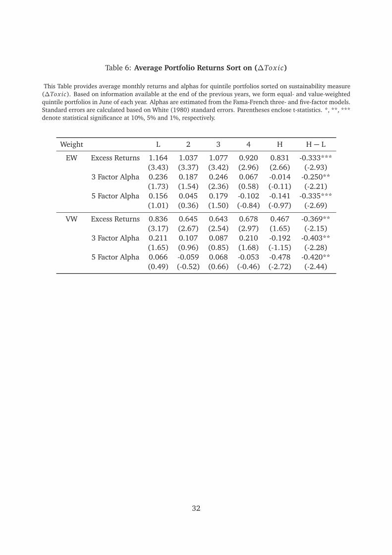
In Table 6, we document the excess returns and alphas of portfolios sorted on ΔToxic.

Consistent with the prediction, we find a significant and negative return spread in the cross-

section. Moving from the lowest to the highest quintile, the average monthly equal-weighted

(EW) excess return decreases from 1.16% to 0.83%. In addition, the difference between the

highest and lowest portfolio returns (-0.33%) is statistically significant at the 1% level. We find

a similar pattern for the value-weighted (VW) results as well, with the high-minus-low return

spread (-0.37%) being slightly wider than the EW spread. Moreover, this decreasing pattern

across quintiles does not seem driven by risk-factor exposures, since we also find significant

and negative alphas for high-minus-low portfolios. For example, when alphas are obtained

from the Fama and French (2015) five-factor model, the difference between the highest and

lowest portfolio alphas are -0.34% (EW) and -0.42% (VW), both of which are significant at

least at the 5% level.

These results imply that a portfolio strategy that takes a long position in a "greener" portfolio

and a short position in a "toxic" portfolio can succeed as a profitable zero-cost strategy. The

17

returns are economically large and not subsumed by risk factors. Riedl and Smeets (2017)

and Barber, Morse and Yasuda (2018) show that investors may be willing to sacrifice financial

returns in exchange for nonpecuniary benefits from investing in funds dedicated to generating

social or environmental benefits. Based on our findings, an important implication can be drawn

if investors have nonpecuniary preferences (Hartzmark and Sussman (2018)). In terms of

investors’ utility, our results suggest that an ESG-preference-based investment strategy achieves

both financial and social objectives.

4.2 Fama-MacBeth Regressions

The results based on portfolio sorts reported in the previous section do not control for other

characteristics that might affect stock returns. In this section, we test whether pollution emis-

sion information earns a premium that is distinct from other firm-level characteristics. We

employ the standard Fama-MacBeth regression approach to control for other firm-level char-

acteristics. We use the following model:

Ri,t+1 = αt + βt ∗ΔToxici,t + C trlsi,t + εi,t+1. (4.1)

The coefficient of interest is βt , which shows how ΔToxic predicts subsequent stock re-

turns. In the specifications, we include several explanatory variables as control variables:

firm size (Size), book-to-market ratio (BM), momentum (Mom), reversal (Rev), book lever-

age (Leverage), capital investment (CAPX/AT), gross profitability (GP), and idiosyncratic risk

(Idiosyn.). Firm-level variables in the regressions are winsorized at the top and bottom 1% to

reduce the influence of outliers. The hypothesis is that we should observe negative coefficients

on ΔToxic when investors consider ESG activity a positive attribute.

In Table 7, we report the estimation results. As seen in column (1), where only ΔToxic is

included, we find the time-series average of coefficients on ΔToxic is -0.551 and statistically

significant at the 1% level. The estimate suggests that a one-standard-deviation increase in

18

ΔToxic (0.4) is associated with a 0.22% greater decrease in returns, which is consistent with

previously reported portfolio results. The negative covariance between pollution abatement

and returns is robust to other controls. In column (2), we include standard controls such as

size, book-to-market, momentum, and reversal. We further add leverage, capital investment,

profitability, and idiosyncratic risk variables and report the results in column (3). In both

specifications, the coefficient estimates are still significantly negative (-0.41 in column(2), -

0.361 in column (3)), implying that the outperformance of greener firms is not likely to be

subsumed by other firm characteristics.

In columns (4) to (6), we include alternative investment measures other than CAPX/AT,

since high ΔToxic is simply a consequence of high investment. Therefore, we consider the

asset growth ratio (AG) in column (4), and the growth rate of CAPX/AT (IG) in column (5).

We also consider the R&D expenditure to asset ratio (XRD/AT) in column (6) because firm-level

ΔToxic may be related to the investment in green technology. In all, the negative coefficient

estimates on ΔToxic seem a robust feature of data.

5 Channels

5.1 Future Firm Performance

In this section, we examine whether polluting behavior also affects firm value and operating

performance to investigate the potential channel for outperformance documented in the previ-

ous section. If our proposed measure of pollution abatement captures firm sustainability that

enhances firm value, we should observe increases in firms’ long-term valuation ratios and sub-

sequent performance. To test the hypothesis, we examine yearly changes in Tobin’s Q, cash

flow, earnings surprise, and gross profitability as measures indicating changes in long-term

valuations and operating performance.

As an additional channel through which greener firms create value, we also consider changes

in institutional ownership exploiting 13F filings data from Thomson Reuters. The rationale be-

19

hind this strategy is to investigate whether cleaner firms attract more institutional investors,

who are relatively long-term investors, resulting in return outperformance documented in the

previous section. To do this, we implement panel regressions as follows:

ΔYi,t+1 = β ∗ΔToxici,t + C trlsi,t + F Es+ εi,t+1. (5.1)

For control variables, we add the logarithm of total assets, leverage, capital investment, and

Tobin’s Q.14 In all specifications, we include industry (based on the Fama-French 48-industry

classification) and year fixed effects. Standard errors are clustered at the industry level.

In Table 8, we report the panel regression results. To obtain the results reported in columns

(1) and (2), we regress the change in Tobin’s Q on ΔToxic and other controls. The coefficient

estimates of -0.036 (column (1)) and -0.021 (column (2)) for ΔToxic indicate a decrease in

firm value in the year after releasing more toxic chemicals. In terms of economic magnitude,

a one-standard-deviation increase in ΔToxic is associated with a 1.44% decrease in Tobin’s Q

(column (1)) compared to an average firm in the sample.

From column (3) to (6), we present the change in operating profits and earnings surprise

as a consequence of toxic release. Similar to Tobin’s Q, we find significant and negative co-

efficients on ΔToxic, indicating that the polluting firms tend to have poorer operating per-

formance and more negative earnings surprise. Greener firms tend to show better earnings

than the analysts’ forecasts. The results collectively suggest that investors initially undervalue

the firms in the greener portfolio, and the realized abnormal returns of the greener firms can

be partially attributable to the investors’ inattention to firm-level earnings growth of greener

firms.

A similar finding is found for gross profitability, and results are reported in columns (7) and

(8). We find that greener firms show outperformance by delivering higher gross profitability in

the following year. A one-standard-deviation increase in ΔToxic predicts a decrease in gross

14Tobin’s Q is excluded from the set of control variables when the change in Tobin’s Q is used as a dependentvariable.

20

profitability by -0.52% (column (5)). To further examine the mechanism behind the outper-

formance of greener firms, we decompose gross profits into revenue and cost and evaluate the

relative importance of cost reduction and revenue enhancement. The estimated results from

column (9) to (12) suggest that the increase in revenue drives the overall change in gross

profitability.

Lastly, in columns (1) and (4) in Table 9, we show that institutional investors on average

reduce their holding of toxic firms after an increase in toxic material release, although the ef-

fect is not far from statistical significance when other controls are included. We then separate

institutional holdings into two groups based on the classification introduced in Bushee (2001),

namely long-term (i.e. "dedicated" institutions) and short-term ("transient" institutions) in-

vestors. It turns out to be that greener firms tend to attract more capital from a subset of

institutional investors who prioritize long-term value creation. We show the results in column

(2) in Table 9. The results on the changes in the average percentage of ownership held by

institutional investors, shown in column (1), seem mainly driven by the changes in holdings

by institutional investors with relatively longer investment horizons rather than investors with

shorter investment horizons.

5.2 Social Trust

When we consider the demand-side explanations for CSR, one can hypothesize that the rela-

tionship between improvements in firm-level sustainability and subsequent returns is stronger

the more the stakeholders of a firm value CSR. Given that firms’ major stakeholders such as

workers, consumers, and shareholders are largely geographically concentrated around its head-

quarters (Coval and Moskowitz (1999)), we capture the base of a firm’s stakeholders as resi-

dents in regions in which a firm is headquartered. To measure the degree of residents’ social

trust, we utilize individual-level survey data and proxy regional level of trust by calculating

the fraction of respondents whose answers are “Most people can be trusted.” We construct an

index of local stakeholders’ social trust at region-year level.

21

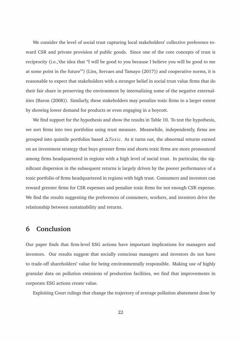
We consider the level of social trust capturing local stakeholders’ collective preference to-

ward CSR and private provision of public goods. Since one of the core concepts of trust is

reciprocity (i.e.,‘the idea that “I will be good to you because I believe you will be good to me

at some point in the future”’) (Lins, Servaes and Tamayo (2017)) and cooperative norms, it is

reasonable to expect that stakeholders with a stronger belief in social trust value firms that do

their fair share in preserving the environment by internalizing some of the negative external-

ities (Baron (2008)). Similarly, these stakeholders may penalize toxic firms to a larger extent

by showing lower demand for products or even engaging in a boycott.

We find support for the hypothesis and show the results in Table 10. To test the hypothesis,

we sort firms into two portfolios using trust measure. Meanwhile, independently, firms are

grouped into quintile portfolios based ΔToxic. As it turns out, the abnormal returns earned

on an investment strategy that buys greener firms and shorts toxic firms are more pronounced

among firms headquartered in regions with a high level of social trust. In particular, the sig-

nificant dispersion in the subsequent returns is largely driven by the poorer performance of a

toxic portfolio of firms headquartered in regions with high trust. Consumers and investors can

reward greener firms for CSR expenses and penalize toxic firms for not enough CSR expense.

We find the results suggesting the preferences of consumers, workers, and investors drive the

relationship between sustainability and returns.

6 Conclusion

Our paper finds that firm-level ESG actions have important implications for managers and

investors. Our results suggest that socially conscious managers and investors do not have

to trade-off shareholders’ value for being environmentally responsible. Making use of highly

granular data on pollution emissions of production facilities, we find that improvements in

corporate ESG actions create value.

Exploiting Court rulings that change the trajectory of average pollution abatement done by

22

firms in the U.S. we find that stricter and broader environmental enforcement create share-

holder value. By examining future stock returns based on a portfolio-based approach, we

show that firms becoming cleaner outperform firms becoming more toxic with similar factor

exposures. By forming quintile portfolios based on toxic releases, we show that investors earn

alpha by taking a long position on a portfolio of the cleanest firms and taking a short position

on the most toxic ones. For value-weighted returns, investors gain 4.3% alpha on the strategy.

We also show that the alphas are driven by the premium earned on firm-level toxic releases.

The announcement returns around the Court rulings and the long-and-short portfolio alphas

are larger for firms located in regions with residents showing higher level of social trust. The

results imply that preferences of stakeholders play a key role in linking CSR and subsequent

returns.

Furthermore, we examine whether pollution abatement is associated with future financial

and valuation performances. We find that firm-level toxic releases are negatively correlated

with Tobin’s Q, cash-flow profitability, gross profitability, and long-term investment among in-

stitutional investors in the next year. Additionally, firm-level sustainability is positively related

to positive earnings surprises. The results suggest that clean firms show enhanced operating

profitability and valuation ratios, which translates into subsequent returns.

Even though information on pollution emissions–the amount of toxic chemical releases

from production facilities– is public and the reporting process is uniformly regulated by envi-

ronmental laws, our results suggest pollution emissions information is slowly capitalized into

stock prices. We show that environmentally conscious investors can construct a financially

profitable strategy based on publicly available information on firm-level sustainability.

23

ReferencesAlbuquerque, Rui, Yrjo Koskinen, and Chendi Zhang. Forthcoming. “Corporate Social Responsibility and Firm

Risk: Theory and Empirical Evidence.” Management Science.

American Lung, Association. 2018. “State of the Air.” Report.

Baker, Malcolm, Daniel Bergstresser, George Serafeim, and Jeffrey Wurgler. 2018. “Financing the Responseto Climate Change: The Pricing and Ownership of U.S. Green Bonds.” National Bureau of Economic ResearchWorking Paper 25194.

Baldauf, Markus, Lorenzo Garlappi, and Yannelis. 2018. “Constantine, Does Climate Change Affect Real EstatePrices? Only If You Believe in it.”

Barber, Brad M., Adair Morse, and Ayako Yasuda. 2018. “Impact Investing.” Working paper.

Baron, David P. 2001. “Private politics, corporate social responsibility, and integrated strategy.” Journal of Eco-nomics & Management Strategy, 10(1): 7–45.

Baron, David P. 2008. “Managerial contracting and corporate social responsibility.” Journal of Public Economics,92(12): 268–288.

Bushee, Brian J. 2001. “Do institutional investors prefer near-term earnings over long-run value?” ContemporaryAccounting Research, 18(2): 207–246.

Chava, Sudheer. 2014. “Environmental externalities and cost of capital.” Management Science, 60(9): 2223–2247.

Cheng, Ing-Haw, Harrison G. Hong, and Kelly Shue. 2016. “Do Managers Do Good with Other Peoples’ Money?”Working Paper.

Choi, Darwin, Zhenyu Gao, and Wenxi Jiang. 2019. “Attention to Global Warming.”

Chowdhry, Bhagwan, Shaun William Davies, and Brian Waters. 2018. “Investing for Impact.” The Review ofFinancial Studies, hhy068.

Cohen, Lauren, Karl Diether, and Christopher Malloy. 2013. “Misvaluing Innovation.” The Review of FinancialStudies, 26(3): 635–666.

Coval, Joshua D., and Tobias J. Moskowitz. 1999. “Home Bias at Home: Local Equity Preference in DomesticPortfolios.” The Journal of Finance, 54(6): 2045–2073.

Di Giuli, Alberta, and Leonard Kostovetsky. 2014. “Are red or blue companies more likely to go green? Politicsand corporate social responsibility.” Journal of Financial Economics, 111(1): 158 – 180.

Dimson, Elroy. 1979. “Risk measurement when shares are subject to infrequent trading.” Journal of FinancialEconomics, 7(2): 197 – 226.

Dimson, Elroy, Oguzhan Karakas, and Xi Li. 2015. “Active Ownership.” The Review of Financial Studies,28(12): 3225–3268.

Dyck, Alexander, Karl V. Lins, Lukas Roth, and Hannes F. Wagner. 2018. “Do institutional investors drivecorporate social responsibility? International evidence.” Journal of Financial Economics.

Edmans, Alex. 2011. “Does the stock market fully value intangibles? Employee satisfaction and equity prices.”Journal of Financial Economics, 101(3): 621 – 640.

Fama, Eugene F., and Kenneth R. French. 1993. “Common risk factors in the returns on stocks and bonds.”Journal of Financial Economics, 33(1): 3–56.

24

Fama, Eugene F., and Kenneth R. French. 2015. “A five-factor asset pricing model.” Journal of Financial Eco-nomics, 116(1): 1 – 22.

Ferreira, Miguel A, and Paul A Laux. 2007. “Corporate Governance, Idiosyncratic Risk, and Information Flow.”Journal of Finance, 62(2): 951âAS989.

Ferrell, Allen, Hao Liang, and Luc Renneboog. 2016. “Socially responsible firms.” Journal of Financial Economics,122(3): 585 – 606.

Flammer, Caroline. 2015. “Does Corporate Social Responsibility Lead to Superior Financial Performance? ARegression Discontinuity Approach.” Management Science, 61(11): 25492568.

Gompers, Paul, Joy Ishii, and Andrew Metrick. 2003. “Corporate Governance and Equity Prices*.” The QuarterlyJournal of Economics, 118(1): 107–156.

Guiso, Luigi, Paola Sapienza, and Luigi Zingales. 2015. “The value of corporate culture.” Journal of FinancialEconomics, 117(1): 60 – 76. NBER Conference on the Causes and Consequences of Corporate Culture.

Hartzmark, Samuel M., and Abigail B. Sussman. 2018. “Do Investors Value Sustainability? A Natural Experi-ment Examining Ranking and Fund Flows.” Working paper.

Karpoff, Jonathan M., Jr. John R. Lott, and Eric W. Wehrly. 2005. “The Reputational Penalties for EnvironmentalViolations: Empirical Evidence.” The Journal of Law & Economics, 48(2): 653–675.

Kelly, Peter. 2015. “Dividends and Trust.” Working paper.

Khotari, S. P, and Jerold B. Warner. 2006. “Econometrics of Event Studies.” B. Espen Eckbo (ed.), Handbook ofCorporate Finance: Empirical Corporate Finance, Volume A (Handbooks in Finance Series.

Kim, Taehyun, and Qiping Xu. 2018. “Financial Constraints and Corporate Environmental Policies.” Workingpaper.

Krüger, Philipp. 2015. “Corporate goodness and shareholder wealth.” Journal of financial economics, 115(2): 304–329.

La Porta, Rafael. 1996. “Expectations and the Cross-Section of Stock Returns.” The Journal of Finance,51(5): 1715–1742.

Larcker, David F., Gaizka Ormazabal, and Daniel J. Taylor. 2011. “The market reaction to corporate governanceregulation.” Journal of Financial Economics, 101: 431 – 448.

Liang, Hho, and Luc Renneboog. 2017. “On the Foundations of Corporate Social Responsibility.” The Journal ofFinance, 72(2): 853–910.

Lins, Karl V., Henri Servaes, and Ane Tamayo. 2017. “Social Capital, Trust, and Firm Performance: The Valueof Corporate Social Responsibility during the Financial Crisis.” The Journal of Finance, 72(4): 1785–1824.

Margolis, Joshua D, Hillary Anger Elfenbein, and James P Walsh. 2011. “Does it pay to be good... and doesit matter? A meta-analysis of the relationship between corporate social and financial performance.” WorkingPaper.

Masulis, Ronald W., and Syed Walid Reza. 2015. “Agency Problems of Corporate Philanthropy.” The Review ofFinancial Studies, 28(2): 592–636.

Murfin, Justin, and Matt Spiegel. 2018. “AIs the Risk of Sea Level Capitalized in Residential Real Estate?”

Novy-Marx, Robert. 2013. “The other side of value: The gross profitability premium.” Journal of Financial Eco-nomics, 108(1): 1 – 28.

25

Riedl, Arno, and Paul Smeets. 2017. “Why Do Investors Hold Socially Responsible Mutual Funds?” The Journalof Finance, 72(6): 25052550.

Schwert, G.William. 1977. “Stock exchange seats as capital assets.” Journal of Financial Economics, 4(1): 51 –78.

Schwert, G. William. 1981. “Using Financial Data to Measure Effects of Regulation.” The Journal of Law & Eco-nomics, 24(1): 121–158.

Servaes, Henri, and Ane Tamayo. 2013. “The Impact of Corporate Social Responsibility on Firm Value: The Roleof Customer Awareness.” Management Science, 59(5): 1045–1061.

Starks, Laura T., Parth Venkat, and Qifei Zhu. 2017. “Corporate ESG Profiles and Investor Horizons.” Workingpaper.

Sugar, Michael. 2007. “Massachusetts v. Environmental Protection Agency.” Harvard Environmental Law Review,31: 531–544.

Tetlock, Paul C. 2011. “All the News That’s Fit to Reprint: Do Investors React to Stale Information?” The Reviewof Financial Studies, 24(5): 1481–1512.

26

Table 1: Average Median Characteristics of Portfolios Sort on (ΔToxic)

This Table reports average characteristics for firms in portfolios formed on the intensity of pollution abatement.Firms are grouped into quintile portfolios sorted by ΔToxic using NYSE breakpoints at the end of each June.

Panel A: Sample Firm CharacteristicsMean Median SD P25 P75 N

ΔToxic 0.020 0.000 0.398 -0.025 0.007 15998log(AT) 6.981 6.904 1.900 5.637 8.243 15998

CAPX/AT 0.060 0.047 0.049 0.028 0.076 15900Leverage 0.263 0.216 0.212 0.092 0.390 15974Tobin’s Q 1.616 1.359 0.839 1.078 1.847 15996

CF 0.150 0.143 0.092 0.097 0.199 15975GP 0.370 0.335 0.206 0.223 0.478 15995

Panel B: Average Median Characteristics of Portfolios Sort on (ΔToxic)All L 2 3 4 H

ΔToxic -0.001 -0.152 -0.016 -0.001 0.004 0.099log(AT) 6.987 6.782 7.239 7.017 7.148 6.824

CAPX/AT 0.046 0.048 0.043 0.043 0.047 0.051Leverage 0.222 0.272 0.219 0.184 0.197 0.254Tobin’s Q 1.359 1.257 1.375 1.463 1.445 1.294

CF 0.142 0.127 0.144 0.149 0.150 0.138GP 0.334 0.285 0.338 0.387 0.364 0.300

Average # Firms 667 138 122 138 133 136

27

Table 2: Announcement Returns Around the Court Decision on April 2, 2007

This Table reports the results on stock price reactions surrounding the Supreme Court rulings on April 2, 2007.

High Δ Toxic is an indicator variable that takes the value of one when firm-level ΔToxic in 2006 comes in above

the median value in the sample of firms reporting to the EPA’s TRI program in 2006 and zero otherwise. Firms withTRI Reporting is an indicator variable that takes the value of one when a firm reports pollution emissions to the

TRI program. Control variables include log of total assets, market leverage ratio, and Tobin’s Q. Standard errors

are clustered at the Fama-French 48 Industry level. Parentheses enclose t-statistics. *, **, *** denote statistical

significance at 10%, 5% and 1%, respectively.

Panel A: Cross-sectional variations in CAR(-1,3)

(1) (2) (3)RawRet(-1,3) CAPM-Adj(-1,3) FF-Adj(-1,3)

High Δ Toxic 0.698∗∗ 0.707∗∗ 0.716∗∗(2.35) (2.23) (2.32)

Observations 601 601 601R2 15.44% 14.74% 14.81%Controls Yes Yes YesFF48 Ind FE Yes Yes YesFF48 Ind Cluster Yes Yes Yes

Panel B: Cross-sectional variations in CAR(-1,10)


High Δ Toxic 0.657∗∗ 0.682∗ 0.714∗∗(2.02) (1.90) (2.11)


Panel C: Robustness


High Δ Toxic 0.696∗∗ 0.703∗∗ 0.712∗∗(2.34) (2.21) (2.30)

Lobbying Firms 0.096 0.203 0.184(0.30) (0.67) (0.59)


28

Table 3: Announcement Returns Around the Court Decision on June 29, 2015

This Table reports the results on stock price reactions surrounding the Supreme Court rulings on June 29, 2015.






Panel A: Cross-sectional variations in CAR(-1,3)


High Δ Toxic -0.753∗∗ -0.673∗∗ -0.669∗(-2.36) (-2.05) (-1.99)


Panel B: Cross-sectional variations in CAR(-1,10)


High Δ Toxic -1.120∗∗ -1.123∗∗ -1.087∗∗(-2.39) (-2.41) (-2.22)


Panel C: Robustness


High Δ Toxic -0.816∗∗ -0.738∗∗ -0.747∗∗(-2.59) (-2.29) (-2.30)

Lobbying Firms -0.686∗ -0.693∗ -0.836∗∗(-1.88) (-1.93) (-2.29)


29

Table 4: Trust and Announcement Returns Around the Court Decision on April 2, 2007

This Table reports the results on stock price reactions surrounding the Supreme Court rulings on April 2, 2007.






Panel A: Announcement Returns in High Trust Regions

(1) (2) (3)RawRet(-1.3) CAPM-Adj(-1.3) FF-Adj(-1.3)

High Δ Toxic 1.134∗∗∗ 1.140∗∗ 1.129∗∗(2.75) (2.45) (2.45)


Panel B: Announcement Returns in Low Trust Regions


High Δ Toxic -0.140 -0.177 -0.147(-0.24) (-0.31) (-0.25)


30

Table 5: Trust and Announcement Returns Around the Court Decision on June 29, 2015

This Table reports the results on stock price reactions surrounding the Supreme Court rulings on June 29, 2015.






Panel A: Cross-sectional Variations in Announcement Returns in High Trust Regions


High Δ Toxic -0.806∗∗ -0.704∗∗ -0.672∗(-2.36) (-2.07) (-1.91)


Panel B: Cross-sectional Variations in Announcement Returns in Low Trust Regions


High Δ Toxic -1.016 -1.144 -1.146(-1.05) (-0.98) (-0.94)


31

Table 6: Average Portfolio Returns Sort on (ΔToxic)

This Table provides average monthly returns and alphas for quintile portfolios sorted on sustainability measure(ΔToxic). Based on information available at the end of the previous years, we form equal- and value-weightedquintile portfolios in June of each year. Alphas are estimated from the Fama-French three- and five-factor models.Standard errors are calculated based on White (1980) standard errors. Parentheses enclose t-statistics. *, **, ***denote statistical significance at 10%, 5% and 1%, respectively.

Weight L 2 3 4 H H − L

EW Excess Returns 1.164 1.037 1.077 0.920 0.831 -0.333***(3.43) (3.37) (3.42) (2.96) (2.66) (-2.93)

3 Factor Alpha 0.236 0.187 0.246 0.067 -0.014 -0.250**(1.73) (1.54) (2.36) (0.58) (-0.11) (-2.21)

5 Factor Alpha 0.156 0.045 0.179 -0.102 -0.141 -0.335***(1.01) (0.36) (1.50) (-0.84) (-0.97) (-2.69)

VW Excess Returns 0.836 0.645 0.643 0.678 0.467 -0.369**(3.17) (2.67) (2.54) (2.97) (1.65) (-2.15)

3 Factor Alpha 0.211 0.107 0.087 0.210 -0.192 -0.403**(1.65) (0.96) (0.85) (1.68) (-1.15) (-2.28)

5 Factor Alpha 0.066 -0.059 0.068 -0.053 -0.478 -0.420**(0.49) (-0.52) (0.66) (-0.46) (-2.72) (-2.44)

32

Table 7: Fama-MacBeth Regressions

This Table provides the second stage Fama-MacBeth regressions of monthly excess stock returns on the sustain-ability measure (ΔToxic) along with a set of controls. Control variables include log market capitalization (Size),log book-to-market ratio (BM), past 12 month stock return skipping the most recent month (Mom), past 1 monthstock return (Rev), capital investment (CAPX/AT), asset growth (AG), investment growth (IG), R&D expenditure(XRD), market leverage (Leverage), gross profitability (GP), idiosyncratic risk (Idiosyn.). Standard errors arecalculated based on White (1980) standard errors. Parentheses enclose t-statistics. *, **, *** denote statisticalsignificance at 10%, 5% and 1%, respectively.

(1) (2) (3) (4) (5) (6)ΔToxic -0.551*** -0.410*** -0.361** -0.372** -0.392*** -0.420***

(-3.28) (-2.80) (-2.52) (-2.55) (-2.69) (-2.90)Size -0.094** -0.089 -0.09 -0.09 -0.084

(-2.02) (-1.37) (-1.39) (-1.39) (-1.31)BM 0.079 0.113 0.089 0.082 0.122

(0.95) (1.30) (1.05) (0.96) (1.54)Mom 0.003 0.003 0.003 0.003 0.002

(0.85) (0.89) (0.90) (0.84) (0.72)Rev -0.034*** -0.037*** -0.036*** -0.036*** -0.036***

(-4.78) (-5.47) (-5.37) (-5.28) (-5.44)CAPX/AT -2.944***

(-2.82)AG -0.689***

(-3.10)IG -5.108***

(-3.75)XRD/AT 5.539***

(2.71)G-Index

E-Index

Leverage 0.176 0.233 0.146 0.114(0.52) (0.69) (0.44) (0.39)

GP 0.691** 0.549* 0.411 0.019(2.09) (1.86) (1.52) (0.21)

Idiosyn. -0.018 -0.011 -0.003 0.279(-0.20) (-0.12) (-0.03) (0.83)

Intercept 0.997*** 1.340*** 1.259 1.141 1.143 0.987(3.23) (2.84) (1.65) (1.46) (1.47) (1.31)

R2 0.28% 5.19% 7.73% 7.61% 7.58% 8.03%Observations 188022 170862 169505 170577 169144 170577

33

Table 8: Long-term Valuation and Financial Performances

This Table reports relationships between sustainability measure, ΔToxic, in year t and various performancemeasures in year t+1. The outcome variables are Tobin’s Q, cash-flow profitability, gross profitability, and earningssurprises. Control variables include log of total assets, leverage, and capital investment. Standard errors areclustered at the Fama-French 48-industry level. Parentheses enclose t-statistics. *, **, *** denote statisticalsignificance at 10%, 5% and 1%, respectively.

(1) (2) (3) (4) (5) (6)ΔQ ΔC F ΔSurprise

ΔToxic -0.036*** -0.021** -0.007** -0.004* -0.004*** -0.004**(-2.95) (-2.06) (-2.26) (-1.70) (-2.84) (-2.68)

Controls No Yes No Yes No YesFF48 Ind FE Yes Yes Yes Yes Yes Yes

Year FE Yes Yes Yes Yes Yes YesFF48 Ind Cluster Yes Yes Yes Yes Yes Yes

R2 12.08% 14.52% 5.53% 9.04% 3.37% 3.57%N 14719 14610 14701 14588 12400 12323

(7) (8) (9) (10) (11) (12)ΔGP ΔRevenue ΔCost

ΔToxic -0.013*** -0.008** -0.035** -0.021* -0.023** -0.014(-2.95) (-2.28) (-2.61) (-1.78) (-2.29) (-1.52)



R2 5.44% 10.86% 7.01% 13.04% 6.77% 11.87%N 14729 14616 14729 14616 14729 14616

34

Table 9: Institutional Investors’ Ownership

This Table reports relationships between sustainability measure, ΔToxic, in year t and institutional ownershipin year t + 1. The outcome variables are percentage of ownership held by institutional investors, institutionalinvestors with longer investment horizons, and institutional investors with shorter investment horizons. Controlvariables include log of total assets, leverage, and capital investment. Standard errors are clustered at the Fama-French 48-industry level. Parentheses enclose t-statistics. *, **, *** denote statistical significance at 10%, 5%and 1%, respectively.

(1) (2) (3) (4) (5) (6)ΔInst.Holdings ΔLong-term ΔShor t-term

ΔToxic -0.011* -0.010 -0.006* -0.007** -0.008 -0.006(-1.69) (-1.44) (-1.90) (-2.10) (-1.46) (-1.05)



R2 12.17% 12.24% 20.86% 20.80% 28.40% 28.90%N 14661 14550 9969 9887 14166 14065

35

Table 10: Average Portfolio Returns Sort on Trust and (ΔToxic)

This Table provides average monthly returns and alphas for portfolios double sorted on trust and sustainabilitymeasure (ΔToxic). In June of each year, based on information available at the end of the previous years, we sortstocks into two portfolios using median value of trust measure. Meanwhile, independently, firms are grouped intoquintile portfolios based on ΔToxic. We form both equal- and value-weighted portfolios. Alphas are estimatedfrom the Fama-French three- and five-factor models. Standard errors are calculated based on White (1980)standard errors. Parentheses enclose t-statistics. *, **, *** denote statistical significance at 10%, 5% and 1%,respectively.

ΔToxic

Weight Type Trust L 2 3 4 H H − L

EW Excess Returns Low 1.076 1.126 1.215 0.903 0.934 -0.142(2.82) (3.19) (3.52) (2.67) (2.65) (-0.89)

High 1.196 0.959 0.909 0.96 0.792 -0.404**(3.36) (2.94) (2.59) (2.88) (2.36) (-2.52)

FF3 Alpha Low 0.171 0.261 0.401 0.077 0.086 -0.085(0.97) (1.86) (2.88) (0.56) (0.53) (-0.53)

High 0.338 0.175 0.087 0.15 -0.01 -0.348**(2.20) (1.15) (0.64) (1.05) (-0.06) (-2.17)

FF5 Alpha Low 0.188 0.137 0.301 -0.108 -0.079 -0.194(0.96) (0.93) (1.87) (-0.74) (-0.44) (-1.13)

High 0.184 -0.028 0.002 -0.095 -0.14 -0.382**(1.12) (-0.17) (0.01) (-0.65) (-0.86) (-2.22)

VW Excess Returns Low 0.935 0.583 0.804 0.859 0.657 -0.278(2.82) (2.13) (3.00) (3.45) (2.10) (-1.09)

High 1.015 0.688 0.667 0.575 0.337 -0.678**(3.57) (2.38) (2.03) (2.19) (0.96) (-2.56)

FF3 Alpha Low 0.311 0.071 0.272 0.394 0.026 -0.285(1.61) (0.38) (1.79) (2.34) (0.13) (-1.17)

High 0.412 0.109 0.032 0.063 -0.398 -0.809***(2.39) (0.70) (0.19) (0.39) (-1.77) (-3.04)

FF5 Alpha Low 0.202 -0.175 -0.007 0.063 -0.223 -0.268(0.97) (-0.97) (-0.05) (0.36) (-1.09) (-1.13)

High 0.171 0.012 0.184 -0.131 -0.628 -0.803***(0.96) (0.08) (1.09) (-0.83) (-2.73) (-2.91)

36

Appendix A: Variable constructionΔToxic is the difference between the amount of total toxic releases in year t and t-1 (Toxic Release - L.ToxicRelease) scaled by the beginning-of-the-year sales (sale).Capx/AT is the ratio of capital expenditure (capex) to beginning-of-the-year book value of assets (at).C F , cash-flow, is defined as income before depreciation and amortization (oibdp) scaled by the beginning-of-the-year book value of assets (at).Leverage is the ratio of total outstanding debt (dlcq+ dl t tq) to beginning-of-the-year book value of assets (at).Tobin′s Q is defined as the market-to-book ratio, where the numerator equals the market value of equity (prccf ∗csho) plus the book assets (at) minus the sum of the book value of common equity (ceq) and deferred taxes andinvestment credit (t xdi tc), and the denominator is the book value of assets (at).Size is log of market capitalization (csho ∗ prccf ).BM is the logarithm of the ratio of the book value of equity to the market value of equity following Fama andFrench (1993).Mom is the 11-month return momentum, skipping the previous month.Rev is the return over the previous month.Idios yn. is the measure of idiosyncratic risk as the ratio of idiosyncratic volatility (obtained from the Fama-Frenchthree-factor model residual) to total volatility, following Ferreira and Laux (2007).AG is the annual change in total assets divided by beginning-of-the-year book value of assets (at).IG is the annual change in capital expenditure (capex) divided by beginning-of-the-year book value of assets(at).XRD/AT is the R&D expenditure (x rd) divided by beginning-of-the-year book value of assets (at). We set thevalue of x rd equal to zero if missing.GP, gross profitability, is the revenues (revt) minus cost of goods sold (cogs) scaled by the beginning-of-the-yearbook value of assets (at).Surprises is the difference between the actual earnings-per-share and the median analyst forecast 3 months priorto the end of the forecast period scaled by stock price on a day before the analyst forecasts.Revenue is the revenues (revt) scaled by the beginning-of-the-year book value of assets (at).Cost is cost of goods sold (cogs) scaled by the beginning-of-the-year book value of assets (at).Inst.Holdings is the proportion of institution holdings reported on 13-F filings.Long-term is the proportion of dedicated holders according to Bushee (2001) reported on 13-F filings.Shor t-term is the proportion of transient holders according to Bushee (2001) reported on 13-F filings.

37

Date post:	07-Feb-2022
Category:	Documents
Upload:	others
View:	3 times
Download:	0 times

Capitalizing on Sustainability: Value of Going Green

Documents