Capturing High-Frequency PhenomenaUsing a Bandwidth-Limited Sensor Network

Ben Greenstein∗ Christopher Mar Alex Pesterev Shahin FarshchiEddie Kohler Jack Judy Deborah Estrin

University of California, Los Angeles{ben, cemar, kohler, destrin}@cs.ucla.edu, alex.p@ucla.edu, {jjudy, shahin}@ee.ucla.edu

ABSTRACT

Small-form-factor, low-power wireless sensors—motes—areconvenient to deploy, but lack the bandwidth to capture andtransmit raw high-frequency data, such as human voices orneural signals, in real time. Local filtering can help, but weshow that the right filter settings depend on changing ambi-ent conditions and network effects such as congestion, whichmakes them dynamic and unpredictable. Mote collection sys-tems for high-frequency data must support iteratively-tuned,deployment-specific filter settings as well as fast sampling.

VANGO, our software system for high-frequency datacollection, achieves these goals via integrated processingacross network tiers. Bandwidth-limited sensor nodes reducedata in network but rely onmicroservers, which have greatercomputational capabilities and a wider scope of observation,to plan how. VANGO provides a cross-platform library fordata transformation, measurement, and classification; a fastand low-jitter data acquisition system for motes; and a mech-anism to control moteand microserver signal processing.With VANGO we have developed new applications: the firstacoustic collection system for motes responsive to chang-ing environmental conditions and user interests, and the firstneural spike acquisition application capable of supporting anetwork of nodes.

Categories and Subject Descriptors:D.2.11 [Software Engineering]: Software Architectures—Domain-specific architectures; C.2.4 [Computer-Commu-nication Networks]: Distributed Systems—Distributed ap-plications; C.2.1 [Computer-Communication Networks]:Network Architecture and Design—Wireless communicationGeneral Terms: Measurement, Performance, Design, Ex-perimentationKeywords: Signal processing frameworks, sensor networks,motes, acoustics, health monitoring

∗Contact author.This material is based in part upon work supported by the National ScienceFoundation under Grant Nos. 0121778 and 0435497. Any opinions, find-ings, and conclusions or recommendations expressed in this material arethose of the author(s) and do not necessarily reflect the views of the Na-tional Science Foundation.Permission to make digital or hard copies of all or part of this work forpersonal or classroom use is granted without fee provided that copies arenot made or distributed for profit or commercial advantage and that copiesbear this notice and the full citation on the first page. To copy otherwise, torepublish, to post on servers or to redistribute to lists, requires prior specificpermission and/or a fee.SenSys’06,November 1–3, 2006, Boulder, Colorado, USA.Copyright 2006 ACM 1-59593-343-3/06/0011 . . . $5.00.

1 INTRODUCTION

Low power wireless sensor platforms have been designedand deployed to support long-lived, inexpensive, unobtrusiveand untethered collection of data from the physical world[13, 15, 25, 26]. Although even the field’s first deployedapplications sampled the environment at much greater spa-tial resolutions than previously possible, they have generallybeen limited to low frequency data (e.g., temperature and hu-midity) [3, 21, 22]. At the urging of their users, these de-ployments [11] tend not to process data in-network in waysthat could potentially lose information; instead they collectall data samples to a resource-rich server, where a researchercan then search for patterns within a complete data set. Atsuch low sampling rates, the benefits of lossy in-network pro-cessing and filtering have not been compelling: there is littledata per node to begin with and most systems have not yethit scaling limits. (Of course,losslesscompression is valu-able even at low sampling rates.)

High-data-rate applications, such as those that involveacoustics, brain waves, seismometers, and imaging, pose newchallenges independent of energy considerations. They pro-duce so much data per node that mote radios, with their ex-treme bandwidth limitations, cannot send that data even onehop in real time. Best-effort collection of such raw data setswill result in significant data loss due to channel contention(presuming a multiple access MAC) and network congestion.Thus, nodes should reduce data before transmission.

If a system must lose data, it is of course better to dis-card data the user wouldn’t want anyway: the system shouldsupportapplication-specific filtering. For instance, the usersof an acoustic network might not be interested in quiet peri-ods. Unfortunately, filter behavior is hard to predict, and ap-plications will perform poorly when filtering is too aggres-sive or otherwise poorly calibrated. Sometimes we know apriori the filter parameters that will collect desired informa-tion while minimizing transmission energy and bandwidth.More often than not, however, engineering systems need tobe tuned while running. Which nodes have interesting datais application- and environment-dependent and time-varying(as our simple experiments confirm). Users interested in thedata that sensor networks produce do not know exactly thebest way to filter it, because they often haven’t seen suchspatially dense data before.

Ideally, then, our sensing system should let us experi-ment with filtering and processing parameters at run time.For instance, when we are calibrating our algorithms, test-ing hypotheses, or simply searching for interesting patternswithin the data, the system could collect raw waveform sam-

1

ples to a user-accessible device with the processing and stor-age capability to perform sophisticated signal analysis: ami-croserver. Bringing waveforms back to a microserver lets useasily explore the consequences of different signal process-ing parameters. When we’ve discovered a suitable set of pa-rameters and signal processing elements implementable onmotes, the system could transfer data processing to the sen-sor nodes themselves, saving bandwidth and increasing theyield of interesting data. Additional tuning will also occur tocompensate for network effects. The calibration process maybe repeated when deployment conditions change, or period-ically, to maintain confidence in our data.

We have constructed VANGO, a TinyOS-based [18] sys-tem for high-rate data collection, around this tuning process.VANGO is quite flexible—it supports several very differentapplications—while being efficient enough to run on smalland very-low-power microcontroller-based sensor nodes. Wemake four contributions: We have developed the first acous-tic collection system for motes that we know of that is flex-ible to changing environmental conditions and user inter-ests, and the first neural spike acquisition application capableof supporting a network of more than two nodes. We havedesigned the software system on which these applicationsrun. This system includes a processing library for data mea-surement, classification, filtering, transformation and com-pression; a fast and low-jitter data acquisition system forresource-constrained motes; and a mechanism to activate andcontrol moteandmicroserver processing of signals. Finally,we demonstrate through experiments the fidelity tradeoffs inbandwidth limited networks. We show that online calibra-tion of our processing algorithms can dramatically improvethe yield of interesting data that is collected; and that in con-gested networks we should filter our data differently than inunconstrained environments.

2 PLATFORM AND APPLICATIONS

Two target applications motivated our work, each of whichcollects data at a high rate. TheAuriclesystem reports acous-tic data, while theNeuromotesystem [4] detects and reportsneural spikes generated, for example, by a rat’s neurons. Bothof these applications are instances of VANGO.

The advantages of a mote including size, cost, deploy-ment flexibility, ability to sleep deeply and wakeup quickly,low energy consumption, and low environmental impact, re-main important for these applications. However, mote-likedevices, including the relatively advanced TelosB mote weuse, cannot continuously transmit at the rates these appli-cations require, and different deployments of either systemmight require different data compression strategies. Our workshows how a software design can collect high-rate data frommotes, even given low-rate radios. This section describes ourhardware platform and applications in more depth.

Sensor platform VANGO applications use networks ofTelosB motes [25]. TelosB is a state-of-the-art platform foruntethered low-power data acquisition. Each TelosB nodehas 10 KB of RAM, a 250 kbps radio, a 12-channel 12-bitADC, and a 16-bit MCU running at 4 MHz with no hard-ware divide or floating point support. For reasons of cost andpower consumption, TelosB motes lack application-specificDSPs that could compress raw data in sophisticated ways.

Radio bandwidth in TelosB networks can be fundamentallyscarce, depending on the number and density of nodes in de-ployment and on the hardware resident on each node. Tradi-tional techniques for signal compression don’t always apply:for instance, GSM could significantly reduce bandwidth foracoustics, but a TelosB cannot run its codec in real time.

Auricle Macroscopic acoustic observations enabled bydense deployments of untethered, unobtrusive sensor nodescould provide scientists with a deeper understanding of wild-life interactions. Proposed acoustic collection projectsin-clude monitoring West Coast acorn woodpeckers and mar-mots [32, 33]. Equally important applications exist in othersettings, such as building monitoring and smart spaces.

Auricle collects acoustic data from a network of motes.Each deployed node consists of a mote connected to an am-plifier and microphone. Nodes are tasked by, and send pro-cessed data back to, a microserver running our software. Ingeneral, Auricle brings to audio monitoring the advantagesof mote-based sensors, including coverage and scale, lowpower consumption, low cost, and easy deployment. Auri-cle is designed to collect raw acoustic waveforms sampled atmore than 8 kHz. (The normal range of adult human hearingis approximately 20 Hz to 16 kHz.) Acoustics have hereto-fore been used by mote-grade platforms primarily for thepurpose of target localization; acoustic waveforms are dis-carded after being measured but before transmission. Inter-esting data is lost. In this sense, Auricle goes beyond theseprior systems [30, 34].

Neuromote Electrophysiological recording is a powerfultool for investigating the mechanisms by which the brain cre-ates and interprets signals. Recordings can help neuroscien-tists understand the brain function that accompanies emo-tions, such as fear and aggression, and diseases, such as epil-epsy and Parkinson’s disease. Neural signals of interest rangefrom an electroencephalogram (EEG), a test to measure elec-trical activity in the brain (on the order of 10 Hz) to hip-pocampal fast ripples, high frequency activity (250–500 Hz)of a population of neurons indicative of the onset of epilepticseizure [1].Spikesare waveforms with a period of a couplemilliseconds that represent the ion discharge of a single neu-ron, which normally occur at a rate of 6–10 Hz [36]. To de-tect neuron spikes, however, a sampling rate of at least 2 kHzis necessary.

Existing wired electrophysiological techniques cannot beused to study freely behaving and interacting test subjectsin an enriched natural and social environment, due to thetethering caused by wires and harnesses. Thus, our Neuro-mote neural sensing application runs on wireless TelosB sen-sor nodes interfaced with test subjects (such as rats) via im-planted depth electrodes and preamplifier circuitry. A Neu-romote attachment restricts rat movement and behavior farless than a wired tethering.

Discussion Any system that collects and transmits dataat such high rates will clearly use a lot of energy. Energy-limited deployments should sample at high rates only occa-sionally—with duty cycling, say, or triggered by some otherevent. We note, however, that Neuromote and similar deploy-ments are not energy-limited as the term is conventionally

2

understood. Long-term disconnected operation is not impor-tant for Neuromote, but form factor and portability require-ments require small batteries too weak to power higher-band-width radios.

3 CASE STUDY

To understand how VANGO is used to filter data in-networkappropriately, we consider a simple Auricle application: col-lecting the sound of a ringing cell phone.

Ideal environment It is easy to detect, isolate, and col-lect a ring heard by a single microphone in a low-noise en-vironment. A mote classifies the captured waveform by itsamplitude—loud sections likely contain ringing while quietsections likely do not—and transmits only the loud sections.

Determining the right threshold between quiet and loudis a matter of estimating the ambient noise level and ac-counting for temporary and unpredictable shifts in that level.In conventional settings, a noise estimator can differentiatenoise from signal automatically, so long as the ambient noiselevel varies slowly and is noticeably below the signal level.In the context of sensor networks, what we consider to benoise—oruninterestingdata—depends on the user. In an en-vironment with guns firing and cell phones ringing, one usermight be interested only in the former, another only in thelatter. Determining the threshold between signal and noisetherefore must be anonline process, because the definitionof noise changes.

When a cell phone rings in a quiet environment, a motethat uses an amplitude classifier can save energy and reduceradio use by discarding sections of the waveform that aren’tloud enough to be interesting. To identify the right thresh-old betweeninterestinganduninteresting, a user could runa sample waveform through a classifier running on a mi-croserver, and when reasonably sure that the chosen clas-sifier and parameters will be effective, activate the classifieron the sensor nodes to save energy.

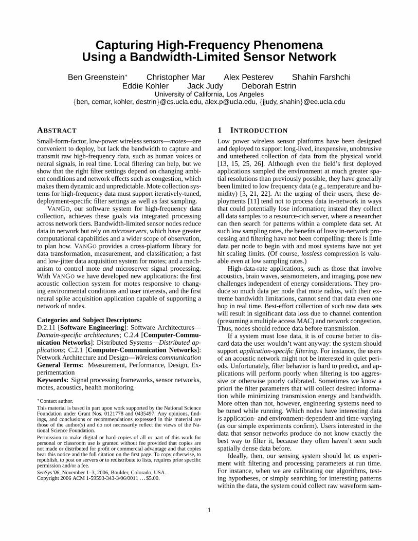
Figure 1 demonstrates this process in VANGO. (See Sec-tion 5 for more detail.) The upper sub-figure shows the acous-tic waveform of a cell phone ringing as sampled by an Au-ricle mote and collected to a microserver. The environmenthas low ambient noise. Analysis on the microserver identifiessufficient classification software (a simple amplitude gate)and parameters (the dashed lines) to detect periods of ring-ing. This information is forwarded to the mote. The lowersub-figure then shows the system’s response to another ring;this time, noise-only periods are pre-filtered out.

-500

0

500

0 2 4 6 8 10 12 14

Time(s)

-500

0

500

Sig

nal (

mV

)

Figure 1—VANGO-collected waveforms with and without amplitude gat-ing. Significant bandwidth and energy are conserved by not transmittinguninteresting portions of the signal.

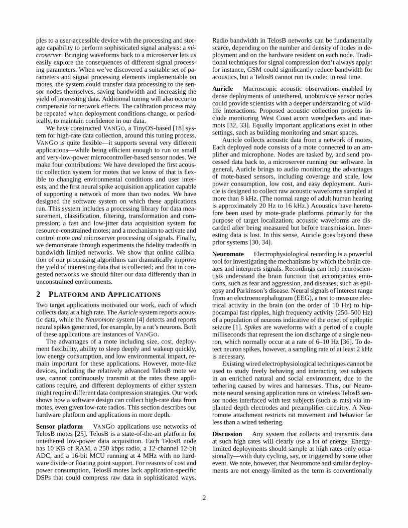
Environmental interference After some time, the ambi-ent noise level may increase until noise is no longer distin-guishable from signal using amplitude alone. More sophis-ticated processing is needed to isolate the interesting por-tions of the signal. A waveform sample could be sent to amicroserver, which has the resources to, for example, definea convolution filter that removes noise and preserves signal,while being simple enough (of small enough order) to oper-ate in real time on motes.1 This filter could be applied to therepresentative waveform in combination with an amplitudeclassifier to test how well the filter and classifier togetherisolate the interesting signal. Once the right parameters arefound, this processing could be activated on the motes.

Figure 2 shows this process in VANGO. No amplitudegate can selectively filter out noise in a noisy environment(top), so the user uses raw waveforms to develop an appro-priate convolution filter (middle). This reveals an amplitudegate level that preferentially selects the signal (dotted lines);installing the filter–gate combination on the motes saves trans-missions (bottom).

-500

0

500

0 2 4 6 8 10 12 14

Time (s)

-500

0

500-500

0

500

Sig

nal (

mV

)

Figure 2—A noisy environment requires an additional convolution filter.

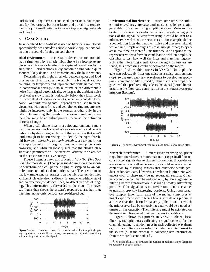
Network interference A microserver receiving cell phonerings from four different motes may notice gaps in all four re-constructed signals due to channel contention. If correlationacross sensors is well understood, we could reduce channelcontention by disabling sensors that otherwise would pro-duce redundant data. However, correlation is often not wellunderstood, or there may be no redundant sensors. Chan-nel contention can then be reduced only by more aggressivefiltering before transmission, discardingweakly interestingportions of the signal so as to provide room on the channelto transmitstrongly interesting portions. Using representa-tive samples taken form each of the motes, a microservermight experiment with filtering levels until data is producedat a rate near the channel’s capacity. (The bitrate at whichthe microserver had been receiving data would be a good es-timate of this capacity.) Then filtering might be activated onthe motes and fine-tuned to actual network conditions.

Figure 3 shows this process in VANGO. Absent localfiltering, multiple motes collecting a signal contend for thechannel, leading to random gaps in each collected waveform(a, b). Local filtering can select for data the mote closest tothe source (c) at the expense of collecting less informationfrom the more distant node (d).

1The order of a filter determines the number of multiplications that mustbe performed on each sample.

3

-500

0

500

0 2 4 6 8 10 12 14

Time (s)

(d)-500

0

500(c)

-500

0

500(b)

-500

0

500(a)

Sig

nal (

mV

)

Figure 3—Collection in the presence of congestion.

4 SYSTEM DESIGN

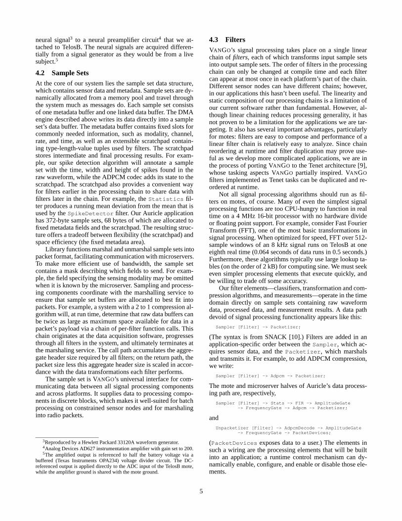
The Auricle and Neuromote applications require support forboth interactive experimentation and long-term collection ofhigh-rate data, and sample formats both uncompressed forprocessing and compressed for transmission. We designedand implemented the VANGO software stack to support theseand other high rate aplications. Its basic abstraction, thesam-ple set, efficiently provides for sample processing and ap-plication-specific format extensions. Each deployed config-uration looks like a single filter chain, simplifying controlmessages (and therefore interactive experimentation) andtheconstruction of new filters. The filter chain abstraction in-troduces several challenges, including how to process time-series data in discrete windows; how to format data passingthrought the system so as to be both flexible and efficient;how to coordinate asynchronous data collection and trans-mission with synchronous data processing; and how to com-bine multiple filters.

Figure 4 describes a typical VANGO software configura-tion. To support tuning and experimentation, the single fil-ter chain spans two platforms. On motes, sensor data is in-jected into the system by our data acquisition software andpushed synchronously in a single call chain down throughthe stack of processing filters. At the terminus of this chainsample sets are marshaled into TinyOS packets and transmit-ted to a microserver via one or more communication hops. Amicroserver uses a TelosB attached via USB as its networkinterface; this passes data packets to VANGO’s microservercode. From there packets are unmarshaled and passed througha similar processing chain, after which the data is exposed toother applications.

4.1 Data AcquisitionThe interrupt load of a sensor network application that inter-acts with an ADC, radio, and timers will induce significantsampling jitter. Furthermore, the interrupt load producedbyan ADC operating at a high rate will overload a system, pre-venting it from doing much else. To collect high-rate data,therefore, we make use of the DMA controller packaged withthe MSP430 MCU on TelosB. We wrote a driver for thisDMA and modified existing TinyOS code to use the DMAto coordinate the transfer of samples from ADC conversionregisters to sequential words in RAM. As opposed to gen-

MSP430ADC12

MSP430DMA

Double Buffer

Buffer Pool

Queue

Queue

*Sample Set

Control

Sampler

Fragment

Amplitude Gate

Frequency Gate

AdPcm

Packetizer

Unpacketizer

Adpcm Decode

Amplitude Gate

Frequency GateControl

Packetizer

Unpacketizer

Packet Devices

EmPdServerEmSocketServer

Queue

Other Library Services

Processing Elements

External Services

< TELOS >

< i686 >

Receive

Send

Send

Receive

Buffer Pool

*Sample Set

MSP430ADC12

MSP430DMA

Double Buffer

Buffer Pool

Queue

Queue

*Sample Set

Control

Sampler

Fragment

Amplitude Gate

Frequency Gate

AdPcm

Packetizer

Unpacketizer

Adpcm Decode

Amplitude Gate

Frequency GateControl

Packetizer

Unpacketizer

Packet Devices

EmPdServerEmSocketServer

Queue

Other Library Services

Processing Elements

External Services

< TELOS >

< i686 >

Receive

Send

Send

Receive

Buffer Pool

*Sample Set

Figure 4—Data and control paths through a VANGO application, includingcode running on a TelosB mote and on a microserver.

erating an interrupt after each sample conversion, the DMAgenerates an interrupt each time it fills a RAM buffer withdata. In order to minimize the latency in providing the DMAwith a new buffer to fill, and hence to decrease the probabil-ity that samples are missed while setting up the next buffer,we prefetch a spare buffer that will be available the instantitis requested.

The sampler operates asynchronously, reacting to theDMA’s interrupts. We place a queue between the samplerand the rest of the system to isolate this asynchrony. Ourqueues are designed to work with dynamically allocated buff-ers; internally, they maintain a circular buffer of pointers tosuch buffers. To avoid polling by those wishing to dequeue,the queue signals when it becomes non-empty.

We run the data acquisition subsystem with compressionsoftware at rates up to 10 kHz. TelosB’s ADC is theoreti-cally capable of generating 200 kilosamples per second. Ifwe do not intend to process or transmit data, our acquisitionsubsystem can sustain rates of up to 115 kHz; insufficientradio bandwidth, however, limits this rate to about 21 kHz(and this presumes that no headers are transmitted and thatthe channel is perfect and available all the time). In practice,without compression, it is difficult to support above 4 kHz.

For Auricle, the data is generated using a low voltagemicrophone preamplifier and an omnidirectional condensermicrophone.2 For Neuromote, we AC-couple a pre-recorded

2SSM2167 from Analog Devices and WM-61A from Panasonic, respec-tively, as suggested by a reference design by Moteiv Corporation.

4

neural signal3 to a neural preamplifier circuit4 that we at-tached to TelosB. The neural signals are acquired differen-tially from a signal generator as they would be from a livesubject.5

4.2 Sample SetsAt the core of our system lies the sample set data structure,which contains sensor data and metadata. Sample sets are dy-namically allocated from a memory pool and travel throughthe system much as messages do. Each sample set consistsof one metadata buffer and one linked data buffer. The DMAengine described above writes its data directly into a sampleset’s data buffer. The metadata buffer contains fixed slots forcommonly needed information, such as modality, channel,rate, and time, as well as an extensible scratchpad contain-ing type-length-value tuples used by filters. The scratchpadstores intermediate and final processing results. For exam-ple, our spike detection algorithm will annotate a sampleset with the time, width and height of spikes found in theraw waveform, while the ADPCM codec adds its state to thescratchpad. The scratchpad also provides a convenient wayfor filters earlier in the processing chain to share data withfilters later in the chain. For example, theStatistics fil-ter produces a running mean deviation from the mean that isused by theSpikeDetector filter. Our Auricle applicationhas 372-byte sample sets, 68 bytes of which are allocated tofixed metadata fields and the scratchpad. The resulting struc-ture offers a tradeoff between flexibility (the scratchpad)andspace efficiency (the fixed metadata area).

Library functions marshal and unmarshal sample sets intopacket format, facilitating communication with microservers.To make more efficient use of bandwidth, the sample setcontains a mask describing which fields to send. For exam-ple, the field specifying the sensing modality may be omittedwhen it is known by the microserver. Sampling and process-ing components coordinate with the marshalling service toensure that sample set buffers are allocated to best fit intopackets. For example, a system with a 2 to 1 compression al-gorithm will, at run time, determine that raw data buffers canbe twice as large as maximum space available for data in apacket’s payload via a chain of per-filter function calls. Thischain originates at the data acquisition software, progressesthrough all filters in the system, and ultimately terminatesatthe marshaling service. The call path accumulates the aggre-gate header size required by all filters; on the return path, thepacket size less this aggregate header size is scaled in accor-dance with the data transformations each filter performs.

The sample set is VANGO’s universal interface for com-municating data between all signal processing componentsand across platforms. It supplies data to processing compo-nents in discrete blocks, which makes it well-suited for batchprocessing on constrained sensor nodes and for marshalinginto radio packets.

3Reproduced by a Hewlett Packard 33120A waveform generator.4Analog Devices AD627 instrumentation amplifier with gain set to 200.5The amplified output is referenced to half the battery voltagevia a

buffered (Texas Instruments OPA234) voltage divider circuit. The DC-referenced output is applied directly to the ADC input of theTelosB mote,while the amplifier ground is shared with the mote ground.

4.3 FiltersVANGO’s signal processing takes place on a single linearchain offilters, each of which transforms input sample setsinto output sample sets. The order of filters in the processingchain can only be changed at compile time and each filtercan appear at most once in each platform’s part of the chain.Different sensor nodes can have different chains; however,in our applications this hasn’t been useful. The linearity andstatic composition of our processing chains is a limitationofour current software rather than fundamental. However, al-though linear chaining reduces processing generality, it hasnot proven to be a limitation for the applications we are tar-geting. It also has several important advantages, particularlyfor motes: filters are easy to compose and performance of alinear filter chain is relatively easy to analyze. Since chainreordering at runtime and filter duplication may prove use-ful as we develop more complicated applications, we are inthe process of porting VANGO to the Tenet architecture [9],whose tasking aspects VANGO partially inspired. VANGOfilters implemented as Tenet tasks can be duplicated and re-ordered at runtime.

Not all signal processing algorithms should run as fil-ters on motes, of course. Many of even the simplest signalprocessing functions are too CPU-hungry to function in realtime on a 4 MHz 16-bit processor with no hardware divideor floating point support. For example, consider Fast FourierTransform (FFT), one of the most basic transformations insignal processing. When optimized for speed, FFT over 512-sample windows of an 8 kHz signal runs on TelosB at oneeighth real time (0.064 seconds of data runs in 0.5 seconds.)Furthermore, these algorithms typically use large lookup ta-bles (on the order of 2 kB) for computing sine. We must seekeven simpler processing elements that execute quickly, andbe willing to trade off some accuracy.

Our filter elements—classifiers, transformation and com-pression algorithms, and measurements—operate in the timedomain directly on sample sets containing raw waveformdata, processed data, and measurement results. A data pathdevoid of signal processing functionality appears like this:

Sampler [Filter] -> Packetizer;

(The syntax is from SNACK [10].) Filters are added in anapplication-specific order between theSampler, which ac-quires sensor data, and thePacketizer, which marshalsand transmits it. For example, to add ADPCM compression,we write:

Sampler [Filter] -> Adpcm -> Packetizer;

The mote and microserver halves of Auricle’s data process-ing path are, respectively,

Sampler [Filter] -> Stats -> FIR -> AmplitudeGate-> FrequencyGate -> Adpcm -> Packetizer;

and

Unpacketizer [Filter] -> AdpcmDecode -> AmplitudeGate-> FrequencyGate -> PacketDevices;

(PacketDevices exposes data to a user.) The elements insuch a wiring are the processing elements that will be builtinto an application; a runtime control mechanism can dy-namically enable, configure, and enable or disable those ele-ments.

5

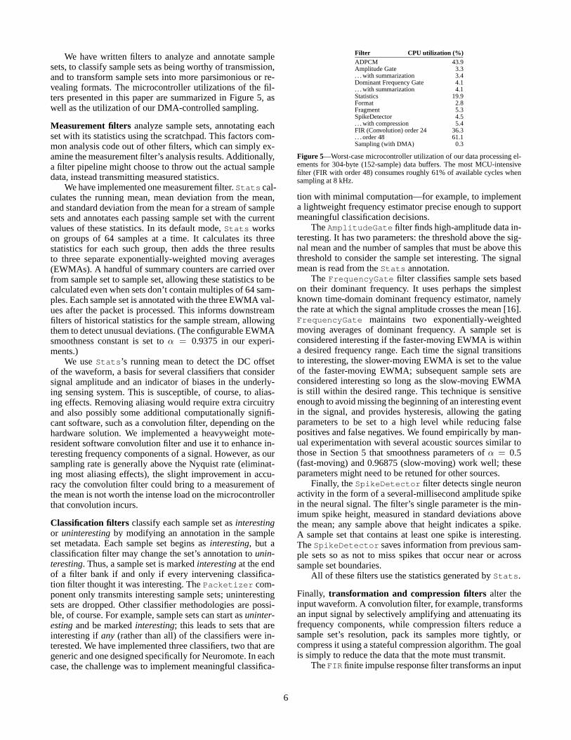
We have written filters to analyze and annotate samplesets, to classify sample sets as being worthy of transmission,and to transform sample sets into more parsimonious or re-vealing formats. The microcontroller utilizations of the fil-ters presented in this paper are summarized in Figure 5, aswell as the utilization of our DMA-controlled sampling.

Measurement filters analyze sample sets, annotating eachset with its statistics using the scratchpad. This factors com-mon analysis code out of other filters, which can simply ex-amine the measurement filter’s analysis results. Additionally,a filter pipeline might choose to throw out the actual sampledata, instead transmitting measured statistics.

We have implemented one measurement filter.Stats cal-culates the running mean, mean deviation from the mean,and standard deviation from the mean for a stream of samplesets and annotates each passing sample set with the currentvalues of these statistics. In its default mode,Stats workson groups of 64 samples at a time. It calculates its threestatistics for each such group, then adds the three resultsto three separate exponentially-weighted moving averages(EWMAs). A handful of summary counters are carried overfrom sample set to sample set, allowing these statistics to becalculated even when sets don’t contain multiples of 64 sam-ples. Each sample set is annotated with the three EWMA val-ues after the packet is processed. This informs downstreamfilters of historical statistics for the sample stream, allowingthem to detect unusual deviations. (The configurable EWMAsmoothness constant is set toα = 0.9375 in our experi-ments.)

We useStats’s running mean to detect the DC offsetof the waveform, a basis for several classifiers that considersignal amplitude and an indicator of biases in the underly-ing sensing system. This is susceptible, of course, to alias-ing effects. Removing aliasing would require extra circuitryand also possibly some additional computationally signifi-cant software, such as a convolution filter, depending on thehardware solution. We implemented a heavyweight mote-resident software convolution filter and use it to enhance in-teresting frequency components of a signal. However, as oursampling rate is generally above the Nyquist rate (eliminat-ing most aliasing effects), the slight improvement in accu-racy the convolution filter could bring to a measurement ofthe mean is not worth the intense load on the microcontrollerthat convolution incurs.

Classification filters classify each sample set asinterestingor uninterestingby modifying an annotation in the sampleset metadata. Each sample set begins asinteresting, but aclassification filter may change the set’s annotation tounin-teresting. Thus, a sample set is markedinterestingat the endof a filter bank if and only if every intervening classifica-tion filter thought it was interesting. ThePacketizer com-ponent only transmits interesting sample sets; uninterestingsets are dropped. Other classifier methodologies are possi-ble, of course. For example, sample sets can start asuninter-estingand be markedinteresting; this leads to sets that areinteresting ifany (rather than all) of the classifiers were in-terested. We have implemented three classifiers, two that aregeneric and one designed specifically for Neuromote. In eachcase, the challenge was to implement meaningful classifica-

Filter CPU utilization (%)ADPCM 43.9Amplitude Gate 3.3. . . with summarization 3.4Dominant Frequency Gate 4.1. . . with summarization 4.1Statistics 19.9Format 2.8Fragment 5.3SpikeDetector 4.5. . . with compression 5.4FIR (Convolution) order 24 36.3. . . order 48 61.1Sampling (with DMA) 0.3

Figure 5—Worst-case microcontroller utilization of our data processing el-ements for 304-byte (152-sample) data buffers. The most MCU-intensivefilter (FIR with order 48) consumes roughly 61% of available cycles whensampling at 8 kHz.

tion with minimal computation—for example, to implementa lightweight frequency estimator precise enough to supportmeaningful classification decisions.

TheAmplitudeGate filter finds high-amplitude data in-teresting. It has two parameters: the threshold above the sig-nal mean and the number of samples that must be above thisthreshold to consider the sample set interesting. The signalmean is read from theStats annotation.

TheFrequencyGate filter classifies sample sets basedon their dominant frequency. It uses perhaps the simplestknown time-domain dominant frequency estimator, namelythe rate at which the signal amplitude crosses the mean [16].FrequencyGate maintains two exponentially-weightedmoving averages of dominant frequency. A sample set isconsidered interesting if the faster-moving EWMA is withina desired frequency range. Each time the signal transitionsto interesting, the slower-moving EWMA is set to the valueof the faster-moving EWMA; subsequent sample sets areconsidered interesting so long as the slow-moving EWMAis still within the desired range. This technique is sensitiveenough to avoid missing the beginning of an interesting eventin the signal, and provides hysteresis, allowing the gatingparameters to be set to a high level while reducing falsepositives and false negatives. We found empirically by man-ual experimentation with several acoustic sources similartothose in Section 5 that smoothness parameters ofα = 0.5(fast-moving) and 0.96875 (slow-moving) work well; theseparameters might need to be retuned for other sources.

Finally, theSpikeDetector filter detects single neuronactivity in the form of a several-millisecond amplitude spikein the neural signal. The filter’s single parameter is the min-imum spike height, measured in standard deviations abovethe mean; any sample above that height indicates a spike.A sample set that contains at least one spike is interesting.TheSpikeDetector saves information from previous sam-ple sets so as not to miss spikes that occur near or acrosssample set boundaries.

All of these filters use the statistics generated byStats.

Finally, transformation and compression filters alter theinput waveform. A convolution filter, for example, transformsan input signal by selectively amplifying and attenuating itsfrequency components, while compression filters reduce asample set’s resolution, pack its samples more tightly, orcompress it using a stateful compression algorithm. The goalis simply to reduce the data that the mote must transmit.

TheFIR finite impulse response filter transforms an input

6

signal by direct convolution in the time domain. This tech-nique takes the sum of the dot product of the filter coeffi-cients with a sliding window of the samples. By designingthe appropriate filter, we can attenuate arbitrary segmentsofthe frequency band. We designed our filters (generated ap-propriate filter coefficients) using GNU Octave signal pro-cessing functions. The direct convolution technique is wellknown and simple to implement, although filtering with fastconvolution using FFT is more common. Because of hard-ware limitations, we only use short filters, for which directconvolution is more efficient than FFT in practice.

TheFormat filter alters the precision and alignment ofsamples within a buffer.Format can reduce sampling pre-cision by truncating 12-bit samples to 8 bits each, or reducewaste by packing pairs of 12-bit samples into 3 bytes each.SinceFormat’s output is a valid sample set, annotated ap-propriately with its precision and alignment,Format mayappear before or after other filters.

The Adpcm filter is an adaptive pulse-code modulationcompressor used in Auricle. Adaptive pulse-code modula-tion is a well-known technique for lossy compression of voicedata. When compared to several other compression schemes,including LPC schemes (GSM 6.10) and simple logarith-mic encoding (u-law), ADPCM has the best combination ofsound quality and compression rate among the few viable forreal-time compression on motes. We use a variant of the In-tel/DVI ADPCM codec, modified to eliminate multiplicationand division operations. Encoding with ADPCM reduces 12-bit ADC samples to 4-bit values. These values are not sam-ples, and cannot be operated on until they are expanded intosamples; thus,Adpcm must occur last in any filter chain ofwhich it is a part. ADPCM is stateful, so to ensure resiliencyto packet loss (and toPacketizer’s refusal to transmit un-interesting sample sets), we include the state of the encoderin each packet as a four-byte header extension.

Finally,SpikeDetector can be configured to compressas well as classify. When configured in spike-only mode, itfilters out baseline noise to produce an abridged version ofthe signal containing only time-referenced spike waveforms.It also measures each spike’s height (amplitude) and width(duration), as these help distinguish the neurons from whichit was generated; the sample set is annotated with these pa-rameters, which might obviate most investigators’ need forthe raw waveform. The resulting data, like that ofAdpcm,uses a special format, so aSpikeDetector in spike-onlymode must occur last in the filter chain.

4.4 Tasking and ControlMotes collect, process, and transmit data. Data reception,training of filter parameters, data refinement, data presenta-tion, and the creation and dispatch of control messages arethe responsibility of the microservers in our network.

Our applications are comprised of two types of executa-bles: one for the deployed motes to acquire and begin pro-cessing the sensor data, and another for the microserver toreceive, finish processing and present it. To help integratethese two executables into a single distributed application,we write all our software modules in nesC [6] and com-pose them into services using SNACK. On microservers, werun nesC code linked to the EmTOS library [7]. From the

perspective of a mote, an EmTOS application appears to beanother mote; however, on the microserver it appears to bea standard Linux process that may interact with other pro-cesses using IPC. Using nesC as the base module descrip-tion language for our entire system simplifies porting dataprocessing algorithms, control interpretation logic, andlinkand routing code from motes to microservers and vice versa.In most cases, the port requires no coding changes.

Individual filters may be activated and deactivated andgiven new parameters at runtime. (A disabled filter passesany sample set it is given to the next filter in the chain with-out performing any processing.) Control over where and howprocessing occurs is determined by a user connected to themicroserver. Processing on the microserver is invoked usingthe same tasking syntax as is used to control deployed motes.

Control of the application is exposed via socket so that ahuman user or controlling application may issue commandsfrom any device with an IP stack. Commands are specifiedin ASCII and have the following syntax:

dest : cmd-name cmd-value [ ; cmd-name cmd-value ]* <CR>

For example, to tell all motes to set their amplitude gatingthreshold to 200 and to enable ADPCM compression, thefollowing suffices:

broadcast: gate-threshold 200; adpcm-enable true

At the time of this writing, there are about 50 commandsdefined in our system.

4.5 Communication PatternsIn single-hop scenarios, control messages are delivered di-rectly to intended recipients, either by unicast or broadcastaddressing. In multi-hop scenarios, for reliability, control mes-sages are flooded using the Drip [19] dissemination protocolirrespective of the destination address. Relative to the band-width consumed by our data traffic, the overhead even offlooding control messages is small.

To avoid expending significant energy buffering sensordata in Flash and to provide acoustics with low latency, datais transmitted by sensor nodes very soon after it is produced.It is collected using the MultiHopLQI routing protocol forTelosB, which is based on Mintroute [39] and supplied aspart of TinyOS 1.x [18]. MultiHopLQI forms a collectiontree with best-effort transport, as opposed to end-to-end re-liability. To support high-rate data transmissions, we mod-ified this code to include a forwarding queue and config-ured the underlying TinyOS link layer to retransmit at mostonce. Presuming a clear channel, on TelosB this link layer’sCSMA MAC supports a transmission rate close to 80 kbps;on crowded links, this rate can be significantly less (e.g.,50 kbps) as backoff delays induce utilization inefficiencies.

5 EVALUATION

This section presents an experimental evaluation of the Au-ricle and Neuromote applications. We demonstrate that it isactually possible to monitor high-rate traffic over low rateradios: our simple and coarse signal processing filters andclassifiers can differentiate interesting data from uninterest-ing data before it is transmitted, and thus reduce networktraffic. In one experiment, traffic was reduced by 78%. Fur-thermore, we can dramatically improve the effectiveness of

7

our collection system through runtime configuration of filter-ing parameters. For instance, by adjusting the gating levelsfor different collections of motes, we can increase the signalenergy we recover by a factor of two.

Our experiments include tests in outdoor and laboratorysettings, using single-link and multi-hop communication ser-vices, and with uniform filter settings as well as settings thatdiffer from node to node. We evaluate the performance ofseveral combinations of processing components, includingAdpcm, Stats, AmplitudeGate, FrequencyGate, andSpikeDetector, and measure the resulting fidelity trade-offs in our networks.

5.1 Auricle: Classifier TuningWe first evaluate how effectively simple local filters can re-duce contention in a densely-deployed sensor network. Wedeploy Auricles sufficiently densely that many nodes can de-tect source phenomena (i.e., noises), albeit with varying fi-delity. We then installAmplitudeGates with varying gatinglevels; this essentially provides us with noise suppression, si-lence elimination, and basic event detection. The evaluationmeasures how much of the source phenomena signal energyis recovered at the sink. Filtering is extremely effective:well-chosen amplitude gate levels can increase this recovered sig-nal energy by factors of 2.5 and more. However, the best am-plitude gate is sensitive to user requirements (demonstratingthe necessity of on-line tuning) and significantly exceeds thelevel of ambient noise.

We chose a general metric—recovered signal energy—to show that effective in-network filtering of high-rate datais highly sensitive to environmental factors, particularly RFavailability. Of course, in specific application contexts,suchas voice recognition or event detection, other metrics wouldbe more telling, like the accuracy of voice reconstruction andpercentage of events detected.

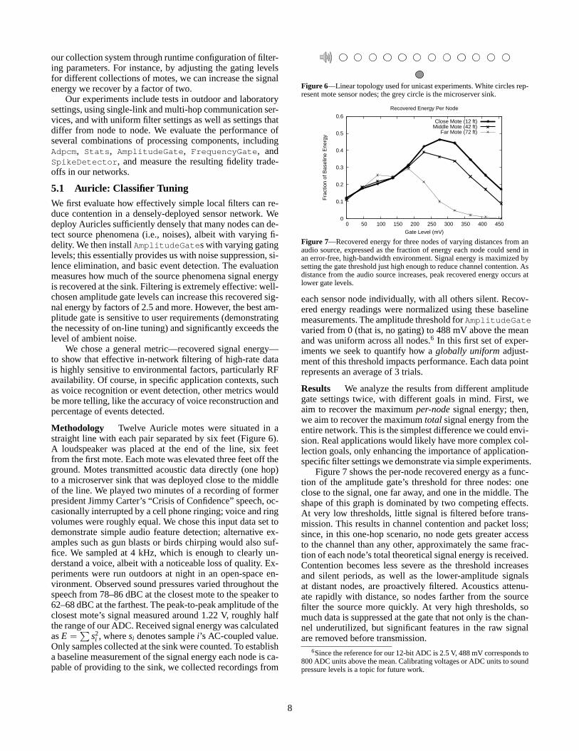
Methodology Twelve Auricle motes were situated in astraight line with each pair separated by six feet (Figure 6).A loudspeaker was placed at the end of the line, six feetfrom the first mote. Each mote was elevated three feet off theground. Motes transmitted acoustic data directly (one hop)to a microserver sink that was deployed close to the middleof the line. We played two minutes of a recording of formerpresident Jimmy Carter’s “Crisis of Confidence” speech, oc-casionally interrupted by a cell phone ringing; voice and ringvolumes were roughly equal. We chose this input data set todemonstrate simple audio feature detection; alternative ex-amples such as gun blasts or birds chirping would also suf-fice. We sampled at 4 kHz, which is enough to clearly un-derstand a voice, albeit with a noticeable loss of quality. Ex-periments were run outdoors at night in an open-space en-vironment. Observed sound pressures varied throughout thespeech from 78–86 dBC at the closest mote to the speaker to62–68 dBC at the farthest. The peak-to-peak amplitude of theclosest mote’s signal measured around 1.22 V, roughly halfthe range of our ADC. Received signal energy was calculatedasE =

∑s2

i , wheresi denotes samplei’s AC-coupled value.Only samples collected at the sink were counted. To establisha baseline measurement of the signal energy each node is ca-pable of providing to the sink, we collected recordings from

Figure 6—Linear topology used for unicast experiments. White circlesrep-resent mote sensor nodes; the grey circle is the microserver sink.

0

0.1

0.2

0.3

0.4

0.5

0.6

0 50 100 150 200 250 300 350 400 450

Fra

ctio

n of

Bas

elin

e E

nerg

y

Gate Level (mV)

Recovered Energy Per Node

Close Mote (12 ft)Middle Mote (42 ft)

Far Mote (72 ft)

Figure 7—Recovered energy for three nodes of varying distances fromanaudio source, expressed as the fraction of energy each node could send inan error-free, high-bandwidth environment. Signal energy is maximized bysetting the gate threshold just high enough to reduce channel contention. Asdistance from the audio source increases, peak recovered energy occurs atlower gate levels.

each sensor node individually, with all others silent. Recov-ered energy readings were normalized using these baselinemeasurements. The amplitude threshold forAmplitudeGatevaried from 0 (that is, no gating) to 488 mV above the meanand was uniform across all nodes.6 In this first set of exper-iments we seek to quantify how aglobally uniformadjust-ment of this threshold impacts performance. Each data pointrepresents an average of 3 trials.

Results We analyze the results from different amplitudegate settings twice, with different goals in mind. First, weaim to recover the maximumper-nodesignal energy; then,we aim to recover the maximumtotal signal energy from theentire network. This is the simplest difference we could envi-sion. Real applications would likely have more complex col-lection goals, only enhancing the importance of application-specific filter settings we demonstrate via simple experiments.

Figure 7 shows the per-node recovered energy as a func-tion of the amplitude gate’s threshold for three nodes: oneclose to the signal, one far away, and one in the middle. Theshape of this graph is dominated by two competing effects.At very low thresholds, little signal is filtered before trans-mission. This results in channel contention and packet loss;since, in this one-hop scenario, no node gets greater accessto the channel than any other, approximately the same frac-tion of each node’s total theoretical signal energy is received.Contention becomes less severe as the threshold increasesand silent periods, as well as the lower-amplitude signalsat distant nodes, are proactively filtered. Acoustics attenu-ate rapidly with distance, so nodes farther from the sourcefilter the source more quickly. At very high thresholds, somuch data is suppressed at the gate that not only is the chan-nel underutilized, but significant features in the raw signalare removed before transmission.

6Since the reference for our 12-bit ADC is 2.5 V, 488 mV corresponds to800 ADC units above the mean. Calibrating voltages or ADC units to soundpressure levels is a topic for future work.

8

0

0.05

0.1

0.15

0.2

0.25

0.3

0 50 100 150 200 250 300 350 400 450

Fra

ctio

n of

Bas

elin

e E

nerg

y

Gate Level (mV)

Total Recovered Energy

Figure 8—Total energy recovered at the sink from all nodes, expressedas the fraction of the energy all nodes could send in an error-free, high-bandwidth environment. The peak occurs at a gate setting of 230 mV, whichdoes not coincide with the maximum received energy of the mote inthebest position to capture the signal (Figure 7). This sharp peak expresses thenetwork-wide point at which congestion effects no longer dominate.

A threshold of 275 mV, the closest node’s peak, willmaximize the maximum per-node recovered energy. This set-ting recovers more than 4.5 times the per-node signal en-ergy of the 0 mV threshold (no gating). Although the generaltrend is intuitive, we expected the maximum signal energyto occur at a threshold just above ambient noise (at about50 mV). The burstiness of human speech is commonly ex-ploited to optimize voice communication systems; we be-lieved that once our gate eliminated the background noisebetween words and syllables, the aggregate received energywould trend quickly upwards. Instead, we found that evenwhen gaps between words were filtered, the remaining traf-fic was still great enough to induce contention-based packetloss and decreased signal yield. Network effects are morepronounced than we had initially expected.

However, users might want a more global metric for yield.Thus, Figure 8 plots the network-widetotal recovered energyfor the experiments of Figure 7. The Y axis shows the totalsignal energy recovered from the network, as a fraction ofthe total signal energy theoretically recoverable. In thisfig-ure, the peak occurs not at the best per-node threshold of275 mV, but rather at 230 mV, which filters somewhat lesssignal from farther nodes. This level recovers approximately2.5 times the signal energy of a system without gates, and ap-proximately 13% more signal energy than the 275 mV gate.

Without a concrete application it is unclear whether 13%more total signal energy matters, but recovering a factor of4.5 or 2.5 more signal energy is important for any collectionapplication we can imagine. The gating levels that lead tothese improvements depend on network topology (becauseof contention), signal characteristics (such as attenuation),and environmental characteristics (such as noise). Not allthese factors can be known in advance of deployment, andmany of them dynamically change, so the ability to dynami-cally adjust the parameters of in-network filters is crucial.

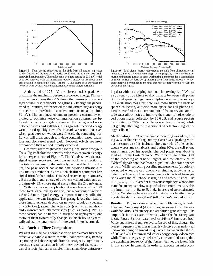
5.2 Auricle: Filter CompositionWe next see whether a combination of simple mote filters caneffectively handle a more complex collection task, namelyseparating cell phone signals from voice signals. High-qualityacoustic signal separation is definitely beyond the capabili-ties of a mote, but can a simpler mechanism drop uninterest-

0

0.05

0.1

0.15

0.2

0.25

0.3

0.35

0.4

0 100 200 300 400 500 600 700 800 900

Fra

ctio

n of

Bas

elin

e E

nerg

y

Minimum Dominant Frequency (Hz)

Total Recovered Energy

Phone: Amp. Gate 245 mVPhone: Amp. Gate 120 mV

Phone: No Amp. GateVoice: Amp. Gate 245 mVVoice: Amp. Gate 120 mV

Voice: No Amp. Gate

Figure 9—Total signal energy recovered at the sink from all nodes, for in-teresting (“Phone”) and uninteresting (“Voice”) signals,as we vary the mini-mum dominant frequency to pass. Optimizing parameters for a compositionof filters cannot be done by optimizing each filter independently. Recov-ered energy is normalized to the total theoretical energy forthe relevant theportion of the signal.

ing data without dropping too much interesting data? We useFrequencyGate filters to discriminate between cell phonerings and speech (rings have a higher dominant frequency).The evaluation measures how well these filters cut back onspeech collection, allowing more space for cell phone col-lection. We find that a combination of frequency and ampli-tude gates allow motes to improve the signal-to-noise ratioofcell phone signal collection by 13.6 dB, and reduce packetstransmitted by 78% over collection without filtering, whilenot greatly affecting the raw amount of cell phone signal en-ergy collected.

Methodology 33% of our audio recording was silent; dur-ing 37% of the recording, Jimmy Carter was speaking with-out interruption (this includes short periods of silence be-tween words and syllables); and during 30%, the cell phonewas ringing over his speech. The cell phone was about asloud as Jimmy Carter’s voice. We refer to that entire 30%of the recording as “Phone” signal, and the other 70% as“Voice” signal; note that Phone signal includes some speechas well. While collecting baseline measurements (as before),we noted when the cell phone was ringing, allowing us todetermine how much recovered energy is derived from pe-riods when the cell phone is ringing and when it is not. TheFrequencyGate classifier filters out sample sets whose dom-inant frequency is below a specified minimum; we vary thisminimum from 0 Hz to 920 Hz in steps of approximately65 Hz. We also include anAmplitudeGate classifier, vary-ing its threshold among 0 mV (off), 120 mV, and 245 mV.

Results Figure 9 shows the amount of Phone signal (solidlines) and Voice signal (dotted lines) recovered from the net-work for various frequency and amplitude gate settings. Theamplitude filter is again effective; when the frequency gateis off, Figure 8’s best gate level of 245 mV improves bothVoice and Phone signal recovery. On top of this, though, thecoarse frequency classifier is clearly effective on signalswithnon-overlapping dominant frequencies: between thresholdsof 200 and 400 Hz, unwanted Voice energy sharply decreaseswhile Phone energy stays relatively constant, indicating thatthe dominant frequency of the former, but not the latter, fallsin this range. In general, in order to execute on microcon-

9

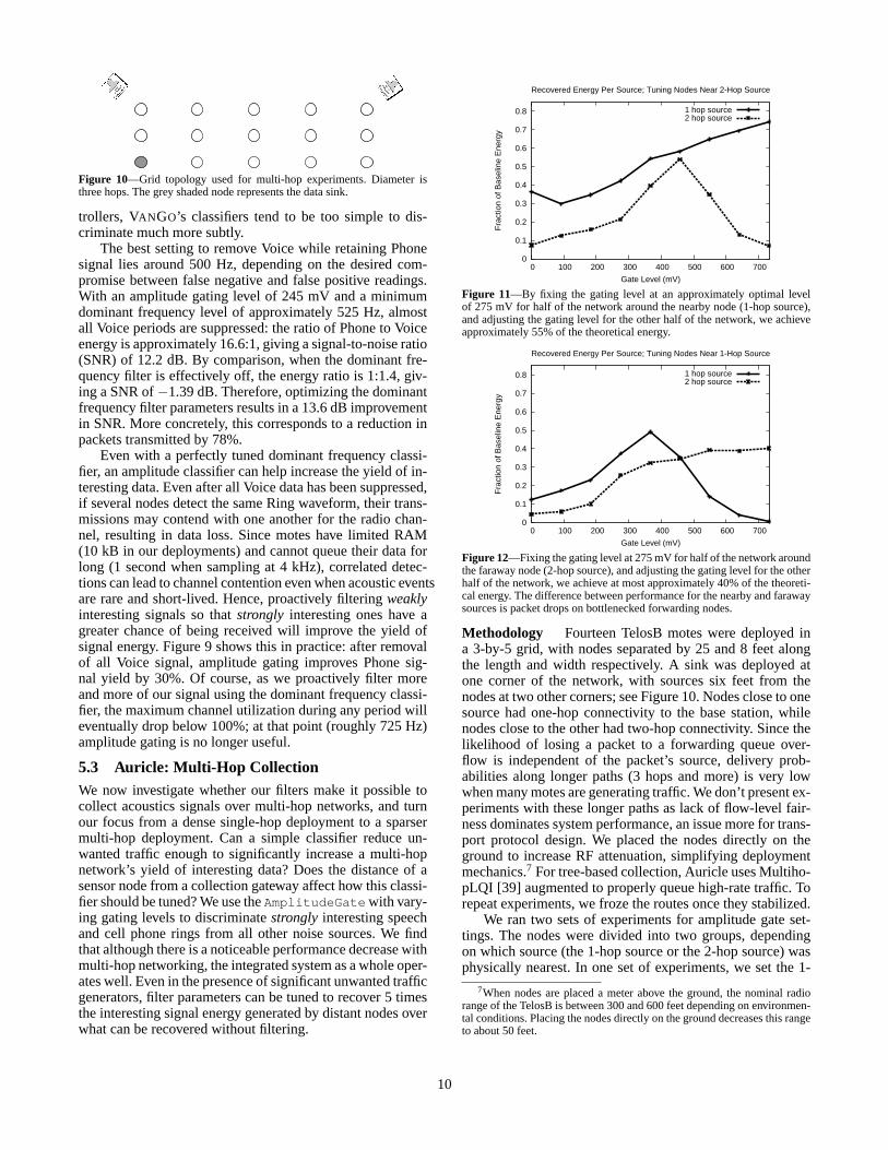
Figure 10—Grid topology used for multi-hop experiments. Diameter isthree hops. The grey shaded node represents the data sink.

trollers, VANGO’s classifiers tend to be too simple to dis-criminate much more subtly.

The best setting to remove Voice while retaining Phonesignal lies around 500 Hz, depending on the desired com-promise between false negative and false positive readings.With an amplitude gating level of 245 mV and a minimumdominant frequency level of approximately 525 Hz, almostall Voice periods are suppressed: the ratio of Phone to Voiceenergy is approximately 16.6:1, giving a signal-to-noise ratio(SNR) of 12.2 dB. By comparison, when the dominant fre-quency filter is effectively off, the energy ratio is 1:1.4, giv-ing a SNR of−1.39 dB. Therefore, optimizing the dominantfrequency filter parameters results in a 13.6 dB improvementin SNR. More concretely, this corresponds to a reduction inpackets transmitted by 78%.

Even with a perfectly tuned dominant frequency classi-fier, an amplitude classifier can help increase the yield of in-teresting data. Even after all Voice data has been suppressed,if several nodes detect the same Ring waveform, their trans-missions may contend with one another for the radio chan-nel, resulting in data loss. Since motes have limited RAM(10 kB in our deployments) and cannot queue their data forlong (1 second when sampling at 4 kHz), correlated detec-tions can lead to channel contention even when acoustic eventsare rare and short-lived. Hence, proactively filteringweaklyinteresting signals so thatstrongly interesting ones have agreater chance of being received will improve the yield ofsignal energy. Figure 9 shows this in practice: after removalof all Voice signal, amplitude gating improves Phone sig-nal yield by 30%. Of course, as we proactively filter moreand more of our signal using the dominant frequency classi-fier, the maximum channel utilization during any period willeventually drop below 100%; at that point (roughly 725 Hz)amplitude gating is no longer useful.

5.3 Auricle: Multi-Hop CollectionWe now investigate whether our filters make it possible tocollect acoustics signals over multi-hop networks, and turnour focus from a dense single-hop deployment to a sparsermulti-hop deployment. Can a simple classifier reduce un-wanted traffic enough to significantly increase a multi-hopnetwork’s yield of interesting data? Does the distance of asensor node from a collection gateway affect how this classi-fier should be tuned? We use theAmplitudeGatewith vary-ing gating levels to discriminatestrongly interesting speechand cell phone rings from all other noise sources. We findthat although there is a noticeable performance decrease withmulti-hop networking, the integrated system as a whole oper-ates well. Even in the presence of significant unwanted trafficgenerators, filter parameters can be tuned to recover 5 timesthe interesting signal energy generated by distant nodes overwhat can be recovered without filtering.

0

0.1

0.2

0.3

0.4

0.5

0.6

0.7

0.8

0 100 200 300 400 500 600 700

Fra

ctio

n of

Bas

elin

e E

nerg

y

Gate Level (mV)

Recovered Energy Per Source; Tuning Nodes Near 2-Hop Source

1 hop source2 hop source

Figure 11—By fixing the gating level at an approximately optimal levelof 275 mV for half of the network around the nearby node (1-hop source),and adjusting the gating level for the other half of the network, we achieveapproximately 55% of the theoretical energy.

0

0.1

0.2

0.3

0.4

0.5

0.6

0.7

0.8

0 100 200 300 400 500 600 700

Fra

ctio

n of

Bas

elin

e E

nerg

y

Gate Level (mV)

Recovered Energy Per Source; Tuning Nodes Near 1-Hop Source

1 hop source2 hop source

Figure 12—Fixing the gating level at 275 mV for half of the network aroundthe faraway node (2-hop source), and adjusting the gating level for the otherhalf of the network, we achieve at most approximately 40% of thetheoreti-cal energy. The difference between performance for the nearby and farawaysources is packet drops on bottlenecked forwarding nodes.

Methodology Fourteen TelosB motes were deployed ina 3-by-5 grid, with nodes separated by 25 and 8 feet alongthe length and width respectively. A sink was deployed atone corner of the network, with sources six feet from thenodes at two other corners; see Figure 10. Nodes close to onesource had one-hop connectivity to the base station, whilenodes close to the other had two-hop connectivity. Since thelikelihood of losing a packet to a forwarding queue over-flow is independent of the packet’s source, delivery prob-abilities along longer paths (3 hops and more) is very lowwhen many motes are generating traffic. We don’t present ex-periments with these longer paths as lack of flow-level fair-ness dominates system performance, an issue more for trans-port protocol design. We placed the nodes directly on theground to increase RF attenuation, simplifying deploymentmechanics.7 For tree-based collection, Auricle uses Multiho-pLQI [39] augmented to properly queue high-rate traffic. Torepeat experiments, we froze the routes once they stabilized.

We ran two sets of experiments for amplitude gate set-tings. The nodes were divided into two groups, dependingon which source (the 1-hop source or the 2-hop source) wasphysically nearest. In one set of experiments, we set the 1-

7When nodes are placed a meter above the ground, the nominal radiorange of the TelosB is between 300 and 600 feet depending on environmen-tal conditions. Placing the nodes directly on the ground decreases this rangeto about 50 feet.

10

hop source group’s gate to 275 mV and varied the gate forthe 2-hop source group; in the other set, we did the reverse,fixing the 2-hop source group’s gate and varying that of the1-hop source group. This procedure was designed to eval-uate the impact of hop distance on optimum gating level.As before, we compare against baselines measured once pernode in the absence of contention; the network-wide baselineenergy is approximately equal for each of the two acousticsources. Each point represents the best result of five trials.

Results Figures 11 and 12 show the results. The maxi-mum total recovered energy, 55% of the theoretical energy,is obtained when the 1-hop and 2-hop source groups haveamplitude gates 275 and 450 mV, respectively; this point isvisible as the 2-hop source’s peak in Figure 11. The gatinglevel for the 2-hop source group is higher than that for the1-hop source group probably because network contentionimpacts multi-hop transmission proportionately more thansingle-hop transmission. This is further visible in the dif-ferences between Figure 11 and 12 at high gating levels:even when all of the 1-hop source’s signal is filtered out, the2-hop source with gating level 275 mV (right-hand side ofFigure 12) achieves less recovered energy than it does witha higher gating level in Figure 11. Aggressive, topology-dependent filtering can thus improve the recovered energyfrom a network, and we have shown that filter tuning canlead to a system that can successfully collect high-rate sig-nals over low-rate radios, even over multiple hops.

5.4 NeuromoteThe Neuromote application collects neural signals in realtime. In this section we study how effectively VANGO canreduce network traffic while still capturing interesting neu-ral spike information. We expect that at high sampling rates,our network does not have the bandwidth to collect completeneuron waveforms from several nodes in real time; however,low sampling rates will result in poor spike detection andcharacterization. Can we use theSpikeDetector filter toaccurately detect and collect spikes from several sources,and can we help a scientist to trust the data? We apply theSpikeDetector and adjust the sampling rate. The evalua-tion measures the key parameters of interest to a scientist:spike heights and widths, as well as the percentage of spikesthat are detected and recovered. We find that with the rightparameters, a Neuromote network can accurately collect neu-ral data from as many as eight concurrently monitored testsubjects. Furthermore, we find that the process of determin-ing the right filtering parameters—interactive and iterativerefinement—also instills a high degree of confidence in thedata the network produces.

Methodology Our experimental setup consists of a wave-form generator programmed to output pre-recorded neuralsignals, a neural preamplifier circuit, and eight TelosB motes.The data programmed into the waveform generator was orig-inally acquired in vivo from freely moving rats.8 Data wererecorded wide band (0.1 Hz to 5 kHz) and sampled at 10 kHz

8Using five four-channel MOSFET input operational amplifiers mountedin the cable connector to remove movement artifacts.

with 12-bit precision.9 The data set corresponds to one sec-ond of neural activity over which there are seven spikes, eachwith an amplitude of 1.85 V (at the motes’ ADC inputs) anda peak-trough duration of approximately 1.34 ms.

We performed two sets of tests. One test measured thepercentage of spikes recovered for different sampling fre-quencies and numbers of motes communicating in the net-work. This test was performed in two modes of operation.In the raw mode, the entire sampled signal was transmittedby each node. In the spike-only mode, motes transmit onlythe portions of the waveform that contain spikes. The secondtest measured the extent of spike parameter variation result-ing from different sampling rates on one to eight motes. Thespike parameters of interest are (a) spike height, which isthe voltage of the acquired signal peak, and (b) spike width,which is the time difference between the spike’s peak voltageand minimum voltage. Spikes that were lost due to packetloss are not accounted for in this test. The sample data usedcontained spikes from a single cell; therefore, each spike wasoriginally equal in amplitude.10

Results Figure 13 describes the percentage of recoveredspikes as a function of the number of nodes in the network atsampling rates of 2 kHz and 8 kHz. When sending the com-plete raw data set, we find that the network has the bandwidthto support one or two motes sampling at 2 kHz, returningnearly 100% of the data pertaining to spikes. However, evenat a 2 kHz sampling rate, with three transmitting motes thespike delivery rate drops off significantly (to under 60%) anddecays to 20% when eight motes are active in the network. Interms of the total number of spikes returned by the network,when sending raw data we find that the maximum spike yieldoccurs with two motes.

In contrast, when spike information is concatenated andthe noise between spikes is removed before transmission, thenetwork performs significantly better. At 2 kHz our yield isabove 90%, even for eight motes. At 8 kHz the network suf-fers a bit from contention and the spike recovery rate decayslinearly from 100% with two motes to under 70% with eightmotes. In terms of the total number of spikes received, wesee that the maximum total spikes recovered (with 8 motes at8 kHz) is roughly two and a half times greater than the max-imum for our raw data experiments (with 2 motes at 2 kHz).

Figure 14 describes the effects of sampling rates on net-works of one, two, and eight motes. Irrespective of whetherraw or abridged waveforms are sent, at below 2 kHz we wit-ness considerable spike loss due to undersampling. This fig-ure again shows that the network can support two nodes’worth of raw data at up to a sampling rate of 2 kHz. This sug-gests that when sending the complete waveform the only op-erating point where nearly all spikes are detected is at 2 kHzwith exactly two motes.

Figure 14 also shows that network congestion penalizesrequests for raw waveforms. This penalty becomes more pro-

9The spikes were isolated from the local field potentials by applying ahigh-pass filter with an f-3dB frequency of 600 Hz. The outputsignals fromthe waveform generator are applied to the neural preamplifiercircuit, whichamplifies and DC references the signals, which are then applied directly tothe ADC inputs of all eight TelosB motes.

10However, the the finite resolution and sampling rate of the original neu-ral signal acquisition apparatus results in a deviation of 108 mV in the dataset that has been programmed into the waveform generator.

11

0

20

40

60

80

100

1 2 3 4 5 6 7 8

Per

cent

Spi

kes

Rec

over

ed

Number of Motes

Number of Motes vs. Spike Recovery in Spike Only Mode

2 kHz spikes only8 kHz spikes only

2 kHz raw data8 kHz raw data

Figure 13—Percentage of recovered spikes as a function of the number ofnodes in the network. In the continuous signal transmission mode (dottedlines), 100% of spikes are only recovered with up to 2 motes, both of whichmust be sampling at 2 kHz. However, when only the waveform containingspike information is transmitted (solid lines), our spike recovery rate is near100% for up to six motes sampling at 2 kHz and always above 65% whensampling at 8 kHz

0

20

40

60

80

100

1000 2000 3000 4000 5000 6000 7000 8000

Per

cent

of S

pike

s R

ecov

ered

Rate (Hz)

Rate vs. Spike Recovery in Spike Only Mode

1 mote spikes only2 motes spikes only8 motes spikes only

1 mote raw data2 motes raw data8 motes raw data

Figure 14—Percentage of recovered spikes as a function of sampling rateand node count in both continuous signal (dotted lines) and isolated spikewaveform (solid lines) transmission modes. In mote modes, spikeloss isobserved below 2 kHz due to under-sampling. At 2 kHz and above,due tochannel contention the spike recovery rate drops with rate,but much lesssignificantly with abridged data. Packet loss is worse for larger networks.

nounced both as the number of motes and as the samplingrate is increased. However, in the isolated spike waveformtransmission mode for 1 and 2 nodes the recovery rate is near100% irrespective of sampling rate. We receive nearly 80%of the spikes when running eight motes in this mode.

Figures 15 and 16 show how the key scientific parametersrecovered from raw waveforms—namely spike widths andheights, respectively—differ as the sampling rate changes.As expected, the greatest amount of variation can be ob-served when the signal is being undersampled (1 kHz). Theparameter variation drops off with increasing sampling fre-quency, leveling off between 2 and 3 kHz for both parame-ters. At 3 kHz the variation of the spike heights and widthsapproach those of the original pre-recorded data set.

Thus, with the right settings—a sampling rate of 2 kHzand transmission of the abridged neural waveforms only—Neuromote can capture the neural spikes from eight subjectsconcurrently and accurately.

Neuromote, like Auricle, shows the tension between fil-ter lossiness and network contention. The right filtering pointdepends on many factors, so a priori knowledge is often in-sufficient to determine the correct filtering parameters. Ourresults shows that system performance follows general trends

0

0.0005

0.001

0.0015

0.002

0.0025

0.003

0.0035

0.004

0 1000 2000 3000 4000 5000 6000

Spi

ke W

idth

(se

cond

s)

Rate (Hz)

Effects of Undersampling on Spike Width

median spike width

Figure 15—Median spike width as a function of sampling rate. The errorbars indicate the 1st and 3rd quartiles. The dotted line at 0.0013 secondsrepresents the median width for all spikes in the input. At frequencies below2 kHz, the variation in the recovered spike widths is high dueto undersam-pling. As the sampling rate is increased, the reported median spike widthconverges to the correct value. Recovering the median spike width with in-creased accuracy enables investigators to classify the cell from which thespike pattern originated with greater precision.

1.2

1.3

1.4

1.5

1.6

1.7

1.8

1.9

0 1000 2000 3000 4000 5000 6000

Spi

ke H

eigh

t Var

iatio

n (V

olts

)

Rate (Hz)

Effects of Undersampling on Spike Height

median spike height

Figure 16—Median spike height as a function of sampling rate. The er-ror bars indicate the 1st and 3rd quartiles. The dotted line at 1.85V repre-sents the actual median height for all spikes in the input. At frequenciesincrease, the accuracy of the reported spike heights increases substantially.Accurate reporting of spike height enables investigators to classify the cellfrom which the spike pattern originated with greater precision.

with respect to filter settings. Thus, a few iterations of onlinetuning will usually yield a significant improvement.

In addition, the collection and tuning process helps sci-entists to trust the system. If nodes transmits filtered data,how can a scientist know if the signal is being accuratelyrepresented? How does the scientist know that the sensor isconnected correctly to a rodent’s brain (in particular, that theattachment isn’t too close to neighboring neurons), that thesampling rate is sufficient for characterization of the signal,and that the network has enough bandwidth to transmit infor-mation from several rodents concurrently? With Neuromote,scientists may collect complete neural waveforms from oneor two nodes and adjust the sampling rate until the signal isverified to be accurate. The network may then be instructedto eliminate periods of noise between neural spikes to savebandwidth.

6 RELATED WORK

6.1 High-Rate Sensor Network ApplicationsSeveral other systems sample at high rates, but usually tar-get very specific applications or system services (localizationin particular), provide few configuration knobs, and collect

12

summary interpretations of the waveform, not the sampledwaveform itself.

Acoustics Acoustic sensor networks are typically factory-tuned to detect specific events. For example, several indoorlocalization systems record ultrasonic pulses for the solepur-pose of noting their times of arrival. Cricket [27], Active-Bat [35], and AHLoS [29] use these times to estimate the dis-tance to a sender. While VANGO does not generate acousticand ultrasonic waveforms, it can detect and timestamp them.More work would be needed to determine if VANGO’s ac-curacy is sufficient for ranging. Likewise, the counter-snip-er system [30] uses mote networks and significant comple-mentary signal processing hardware (an FPGA on a custom-designed sensor board) to detect gunshots and localize theirsources. While VANGO’s spike detection software could beapplied to detect gunshots, the 1 MHz required sampling rateto perform fine-grained acoustic localization is beyond thecapabilities of the mote hardware VANGO uses. VigilNet [12],a sensor network surveillance system, uses dual axis mag-netometers, microphones, accelerometers, and photo sensorsto detect similarly application-specific events and then sendnotifications. It can trade detection sensitivity for longevity,but its design is otherwise rigid. VigilNet’s vehicle detectionlogic, wakeup message format, logic to define the group ofnodes that are to be recipients of such messages, protocol forduty-cycled rendezvous, and in-network cooperating aggre-gation of tracking messages are all application-specific andcomplicated; reusing the code in new applications will bedifficult. This contrasts the work of VANGO, which providessoftware that is more generic and reusable. Finally, ENS-Box [8] is a flexible platform for prototyping rapidly deploy-able acoustic sensing systems that do significant in-networkprocessing. Unlike VanGo, it is built atop Linux and is de-signed with greater computational capabilities (ARM hard-ware) in mind.

Biological signals The CodeBlue [20] project has devel-oped mote-based sensors with biological interface circuits,some similar to those used for VANGO’s neural monitoringapplication. These nodes have been used to acquire and wire-lessly transmit biological signals, including pulse oximetryand electrocardiogram (EKG) data. CodeBlue, however, wasnot designed to acquire and filter data at the rates necessary,for example, to obtain and transmit neural spike activity. TheEKG waveform, for example, is typically sampled at 120 Hz.

Other high-rate phenomena The Cyclops imaging sys-tem [28] produces low-frequency data but at a high resolu-tion. Data reduction before transmission is thus often key topromoting network longevity and meeting available band-width. Cyclops is capable of performing a range of data ac-quisition and manipulation options, but it has not yet beensuccessful in exposing this functionality in a manner whichcan be composed at runtime to meet new application tasks;we hope the data structures and filter organization of VANGOwill be helpful in this regard.

Accelerometers and cheaper seismoacoustic sensors havebeen used in structural monitoring and the measurement ofseismic activity. Werner-Allen et al. [37, 38] deployed twomote-based seismic arrays on volcanoes in Ecuador. Theirnodes sample at roughly 100 Hz. To reduce data in-network,

they use a detector similar to VANGO’s spike detector. Kimet al. [17] monitored ambient vibration of the Golden GateBridge using Mica2 motes and custom accelerometer boards.Using carefully written embedded code, they were able toachieve a sampling rate of 200 Hz with relatively low jitter—much less of a problem with the newer TelosB mote andDMA-based data acquisition software of VANGO. Likewise,Wisden [41], a system for reliably transporting structuralvi-bration data from a collection of sensors to a base station,incorporates Mica2 motes and a vibration card (accelerom-eter), samples at a high rate (100Hz), and delivers data re-liably over multiple hops to a base station where it can bevisualized.

6.2 Signal Processing FrameworksMany other signal processing compositional frameworks ex-ist. These systems typically offer extensive high-level librariesand streamlined user interfaces. Their sophisticated user-levelsupport is complementary to the work of VANGO. Whilethey are sometimes capable of producing code for embed-ded platforms, they are not designed explicitly for operationon distributed microcontroller-based wireless sensing sys-tems. Labview is a platform with a visual dataflow languageused for data acquisition, industrial automation, and instru-ment control [14]. Labview applications depend on a runtimeengine and libraries designed for PCs. Simulink [23] andPtolomy II [2] are visual component composition systems formodeling control and signal processing applications. WhenSimulink is used with the real-time processing toolbox, itcan generate high performance code that is suitable for con-strained embedded systems. Similarly, Ptolemy applicationscan be compiled for an embedded target. StreamIt [31] isa language and compiler for generating real-time streamingsystems on embedded platforms. It supports general purposeuniprocessors and the MIT Raw machine.

6.3 Internet and Cellular TranscodingThe problem of reducing high-rate data to alleviate networkcongestion has been studied extensively in the context of In-ternet and cellular transcoding [5, 24, 40]. VANGO sharesone goal in particular with these projects, maximizing appli-cation performance given bandwidth constraints. Unlike theprevious work, however, a sensor network application com-petes with itself for bandwidth. This property alone can leadto finer control over how data is collected and filtered, be-cause a sensor network application can make network-widedecisions about how to allocate and use bandwidth.

7 CONCLUSION

We have designed a heterogeneous software system capableof high-rate data acquisition and single- and multiple-hopwireless transmission. Not only does it efficiently process,classify, measure, compress, and transform raw sensor data,but it also provides cross-tier mechanisms to help users cal-ibrate the system while it is running and thus improve itsperformance. We presented high-rate collection applicationsin two domains, acoustics and neurophysiological monitor-ing. In both applications, simple filters can impact network

13

performance greatly, particularly in bandwidth-limited envi-ronments. As we have shown with both applications, selec-tive and informed filtering before transmission yields moreof the data that interests a user. A system designed around theneeds of both high-rate sampling and flexible runtime filtertuning makes the benefits of mote data collection accessibleeven to high-data-rate applications.

ACKNOWLEDGMENTS

We would like to thank our reviewers and our shepherd, SamMadden, for valuable feedback; Mohammad Rahimi for hard-ware support; and the TinyOS and Emstar communities forsoftware contributions.

REFERENCES[1] A. Bragin, J. Engel, C. L. Wilson, I. Fried, and G. W. Mathern. Hip-

pocampal and entorhinal cortex high-frequency oscillations (100–500Hz) in human epileptic brain and kainia acid-treated rates with chronicseizures.Epilepsia, 40:127–137, February 1999.

[2] J. Buck, S. Ha, E. A. Lee, and D. G. Messerschmitt.Ptolemy: A frame-work for simulating and prototyping heterogeneous systems, pages527–543. Kluwer Academic Publishers, Norwell, MA, USA, 2002.

[3] A. Cerpa, J. Elson et al. Habitat monitoring: Applicationdriverfor wireless communications technology. InProc. 2001 ACM SIG-COMM Workshop on Data Communications in Latin America and theCaribbean, April 2001.

[4] S. Farshchi, P. H. Nuyujukian, A. Pesterev, I. Mody, and J. W. Judy.A TinyOS-based wireless neural sensing archiving and hosting sys-tem. InProc. 2nd International IEEE EMBS Conference on NeuralEngineering, March 2005.

[5] A. Fox, S. D. Gribble, Y. Chawathe, E. A. Brewer, and P. Gauthier.Cluster-based scalable network services. InProc. 16th ACM Sympo-sium on Operating Systems Principles, pages 78–91, Oct. 1997.

[6] D. Gay, P. Levis et al. The nesC language: A holistic approach tonetworked embedded systems. InProc. ACM SIGPLAN 2003 Confer-ence on Programming Language Design and Implementation (PLDI),pages 1–11, June 2003.

[7] L. Girod, T. Stathopoulos et al. A system for simulation, emulation,and deployment of heterogeneous sensor networks. InProc. 2nd ACMSenSys Conference, pages 201–213, Nov. 2004.

[8] L. Girod, M. Lukac, V. Trifa, and D. Estrin. The design andimple-mentation of a self-calibrating distributed acoustic sensing platform.In Proc. 4th ACM SenSys Conference, Nov. 2006.

[9] O. Gnawali, B. Greenstein et al. The Tenet architecture for tieredsensor networks. InProc. 4th ACM SenSys Conference, Nov. 2006.

[10] B. Greenstein, E. Kohler, and D. Estrin. A sensor network applicationconstruction kit (SNACK). InProc. 2nd ACM SenSys Conference,pages 69–80, Nov. 2004.

[11] R. Guy, B. Greenstein et al. Experiences with the Extensible SensingSystem ESS. Technical Report 61, CENS, UCLA, Mar. 29 2006.

[12] T. He, S. Krishnamurthy et al. VigilNet: An integrated sensor networksystem for energy-efficient surveillance. InProc. 3rd ACM SenSysConference, Nov. 2005.

[13] C. T. Inc.http://www.xbow.com/.[14] N. Instruments. Labview – the sofware that powers virtual instrumen-

tation.http://www.ni.com/labview/.[15] J. Kahn, R. Katz, and K. Pister. Next century challenges: Mobile net-

working for Smart Dust. InProc. 5th Annual International Confer-ence on Mobile Computing and Networking (MobiCom ’99), pages271–278, Aug. 1999.

[16] B. Kedem. Spectral analysis and discrimination by zero-crossings.P-IEEE, 74:1477–1493, 1986.

[17] S. Kim. Wireless sensor networks for structural health monitoring.Master’s thesis, University of California, Berkeley, 2005.

[18] P. Levis, S. Madden et al. The emergence of networking abstractionsand techniques in TinyOS. InProc. 1st Symposium on NetworkedSystems Design and Implementation (NSDI ’04), pages 1–14, Mar.2004.

[19] P. Levis, N. Patel, D. Culler, and S. Shenker. Trickle: Aself-regulatingalgorithm for code propagation and maintenance in wireless sensornetworks. InProc. 1st Symposium on Networked Systems Design andImplementation (NSDI ’04), Mar. 2004.

[20] K. Lorincz, D. J. Malan et al. Sensor networks for emergency re-sponse: Challenges and opportunities.IEEE Pervasive Computing,October–December 2004.

[21] S. Madden, M. Franklin, J. Hellerstein, and W. Hong. TAG: A TinyAGgregation service for ad-hoc sensor networks. InProc. 5th Sympo-sium on Operating Systems Design and Implementation (OSDI ’02),Dec. 2002.

[22] A. Mainwaring, J. Polastre, R. Szewczyk, D. Culler, andJ. Anderson.Wireless sensor networks for habitat monitoring. InProc. 1st ACM In-ternational Workshop on Wireless Sensor Networks and Applications(WSNA), Sept. 2002.

[23] MathWorks. Simulink – simulation and model-based design.http://www.mathworks.com/products/simulink/.

[24] S. McCanne, V. Jacobson, and M. Vetterli. Receiver-driven layeredmulticast. InProc. ACM SIGCOMM ’96 Conference, pages 117–130,Aug. 1996.

[25] J. Polastre, C. Sharp, and R. Szewczyk. URLhttp://www.moteiv.com. Moteiv website.

[26] G. J. Pottie and W. J. Kaiser. Embedding the Internet: Wireless inte-grated network sensors.Communications of the ACM, 43(5):51–58,May 2000.

[27] N. B. Priyantha, A. Chakraborty, and H. Balakrishnan. The cricketlocation-support system. InProc. 6th Annual International Confer-ence on Mobile Computing and Networking (MobiCom 2000), Aug.2000.

[28] M. Rahimi, D. Estrin, R. Baer, H. Uyeno, and J. Warrior. Cyclops,image sensing and interpretation in wireless networks. InProc. 2ndACM SenSys Conference, pages 311–311, Nov. 2004.

[29] A. Savvides, C.-C. Han, and M. B. Srivastava. Dynamic fine-grainedlocalization in ad-hoc networks of sensors. InProc. 7th Annual In-ternational Conference on Mobile Computing and Networking(Mobi-Com 2001), pages 166–179, July 2001.

[30] G. Simon, M. Maroti et al. Sensor network-based countersniper sys-tem. InProc. 2nd ACM SenSys Conference, pages 1–12, Nov. 2004.

[31] W. Thies, M. Karczmarek, and S. Amarasinghe. StreamIt: A languagefor streaming applications. InProc. 2002 International Conference onCompiler Construction, pages 179–196, April 2002.

[32] V. M. Trifa. A framework for bird songs detection, recognition andlocalization using acoustic sensor networks. PhD thesis, Ecole Poly-technique Federale de Laussanne and University of California, LosAngeles, 2006.

[33] H. Wang, C. Chen et al. Acoustic sensor networks for woodpeckerlocalization. InSPIE Conference on Advanced Signal Processing Al-gorithms, Architectures and Implementations, Aug. 2005.

[34] Q. Wang, W. Chen, R. Zheng, K. Lee, and L. Sha. Acoustic tar-get tracking using tiny wireless sensor devices. InProc. 2nd Inter-national Symposium on Information Processing in Sensor Networks(IPSN ’03), pages 642–657, Apr. 2003.

[35] A. Ward, A. Jones, and A. Hopper. A new location technique for theactive office. IEEE Personnel Communications, 4(5):42–47, October1997.

[36] P. T. Watkins, G. Santhanam, K. V. Shenoy, and R. R. Harrison. Val-idation of adaptive threshold spike detector for neural recording. InProc. 26th International Conference of the IEEE EMBS, pages 4079–4083, 2004.

[37] G. Werner-Allen, J. Johnson, M. Ruiz, J. Lees, and M. Welsh. Moni-toring volcanic eruptions with a wireless sensor network. In Proc. 2ndEuropean Workshop on Wireless Sensor Networks, January–February2005.

[38] G. Werner-Allen, K. Lorincz et al. Deploying a wirelesssensor net-work on an active volcano.IEEE Internet Computing, March–April2006. Special Issue on Data-Driven Applications in Sensor Networks.

[39] A. Woo, T. Tong, and D. Culler. Taming the underlying challenges ofreliable multihop routing in sensor networks. InProc. 1st ACM SenSysConference, Nov. 2003.

[40] D. Wu, A. Swan, and L. A. Rowe. Internet MBone broadcast manage-ment system. InProc. ACM SIGMultimedia Conference on Multime-dia Computing and Networking, 1999.

[41] N. Xu, S. Rangwala et al. A wireless sensor network for structuralmonitoring. InProc. 2nd ACM SenSys Conference, Nov. 2004.

14